Compressive response and helix formation of a semiflexible polymer confined in a nanochannel

Abstract

Configurations of a single semiflexible polymer is studied when it is pushed into a nanochannel in the case where the polymer persistence length $l_{p}$ is much longer than the channel diameter $D$, i.e. $l_{p}/D\gg 1$. Using numerical simulations, we show that the polymer undergoes a sequence of recurring structural transitions upon longitudinal compression, i.e. random deflection along the channel, helix going around the channel wall, double-fold random deflection, double-fold helix, etc. We find that the helix transition can be understood as buckling of deflection segments, and the initial helix formation takes place at very small compression with no appreciable weak compression regime of the random deflection polymer.

I introduction

The behavior of semiflexible polymers in confined spaces is interesting for various reasons. Consider a polymer with the persistence length $l_{p}$ and the contour length $L$, which is confined in the space with the characteristic size $D$. The degree of confinement can be quantified by the ratio $D/R$, where $R$ is the natural size of the chain in bulk, i.e. $R\simeq l_{p}(L/l_{p})^{1/2}$ for an ideal chain. For polymers which are flexible down to the scale of molecular thickness $a$, i.e. $l_{p}/a\sim 1$, it is indeed possible to construct a scaling theory on the behavior of confined polymer based solely on the ratio $D/R$ de Gennes (1977); Grosberg and Khokhlov (1994); Sakaue and Raphael (2006). In contrast, the large persistence length $l_{p}/a\gg 1$ in semiflexible polymers introduces an additional measure $D/l_{p}$ for the degree of confinement, which leads to a rich variety of scenarios both in nanochannel/slit Chen and Sullivan (2006); Odijk (2008); Reisner et al. (2012); Chifra (2012); Wang et al. (2011); Huang and Bhattacharya (2014); Werner and Mehlig (2015) and in closed cavity Sakaue (2007); Klotz et al. (2015). Examples of current hot topics include the elongation of DNA in nanoscale channels Reisner et al. (2012) and the constrained dynamics of actin filaments and microtubles in cytoskeletal network Köster et al. (2005); Gardal et al. (2008). The former is becoming an indispensable technique in single molecule genomics, and the latter largely dictates the rheological behavior of cells. In such fields of single molecule biophysics, a rapid progress in molecular visualization and manipulation techniques to smaller and smaller length scale is continuously stimulating the study on statistical mechanical description of confined semiflexible polymers.

In this report, we consider the situation, in which a semiflexible polymer confined in a nanochannel is compressed by a sliding piston as shown in Fig. 1. If the polymer is flexible at the scale of confinement, i.e. $l_{p}/D\ll 1$, the polymer is compressed randomly, developing a dense pile of blobs analogous to those in a semidilute solution Sakaue and Raphael (2006); Jun et al. (2008). Our focus here is on the opposite limit $l_{p}/D\gg 1$, where a random folding state is energetically disfavored. Although the statistics of a semiflexible polymer in such a narrow channel is now rather well understood as Odijk regime Odijk (1983), the response to the compressive force has not been addressed yet. Using Langevin dynamic simulation, we show that in such a case the polymer transforms from a random deflection configuration into an ordered helix structure upon compression. Further compression leads to destabilization of the helix into a double-fold random deflection, then the second buckling takes place to form the double-fold helix. We expect that such a sequence of recurring structural transitions is within reach using nano-piston experiment set-up Khorshid et al. (2014, 2016); Reccius et al. (2005); Pelletier et al. (2012), and its investigation offers interesting challenges to explore rich confinement scenarios realized in the halfway between nanochannel and closed cavity geometries, where the effective spacial dimensionality changes from one to zero.

II model

In numerical simulations, we employ a coarse-grained model of semiflexible polymer, which is made of $N$ successive beads with diameter $\sigma$. All beads interact through a shifted purely repulsive Lennard-Jones potential $U^{LJ}$,

$$U^{LJ}(r)=\begin{cases}\displaystyle 4\epsilon\left[\left\{\frac{\sigma}{r}\right\}^{12}-\left\{\frac{\sigma}{r}\right\}^{6}+\frac{1}{4}\right]&r<2^{{1}/{6}}\sigma\\ 0&r>2^{{1}/{6}}\sigma\end{cases},$$ (1)

where $r$ is the inter-bead distance, and $\epsilon$ sets the energy scale. The linear connectivity of the chain is ensured by the Finitely-Extensible-Nonlinear-Elastic potential $U^{s}$ between neighboring beads Grest and Kremer (1986),

$$U^{s}(r)=-\frac{1}{2}k_{s}r_{0}^{2}\ln{\left[1-\bigg{(}\frac{r}{r_{0}}\bigg{)}^{2}\right]}.$$ (2)

Finally, the stiffness of the chain is controlled via the bending potential

$$U^{b}(\theta)=\frac{\kappa}{\sigma}\,(1-\cos\theta),$$ (3)

with $\theta$ being the angle between two consecutive bonds along the chain. The chain therefore approximates the worm-like chain with the persistence length $l_{p}=\kappa/k_{B}T$, where $k_{B}T$ is the thermal energy.

The chain is confined in the cylindrical channel with two end caps, whose size is characterized by its cross sectional diameter $D$ and the axial length $X$. To compress the chain, the cap at $x=X(t)$ moves with a constant velocity $c$ in the $-x$-direction with the cap at $x=0$ being fixed, where we set the channel axis to be the $x$-axis. The surface of such a confining geometry is implemented via the potential $U^{c}$, for which we also use $U^{LJ}$ of Eq. (1). Note that the distance $r$ in this case is form the cylinder wall, whose diameter is set to be $D+2\sigma$ so that the effective diameter for the beads should be $D$.

The position ${\mbox{\boldmath$r$}}_{i}=(x_{i},y_{i},z_{i})$ of the $i$-th bead evolves with time according to Langevin equation

$$m\frac{d^{2}{\mbox{\boldmath$r$}}_{i}}{dt^{2}}=-\nabla_{i}U-\Gamma\frac{d{\mbox{\boldmath$r$}}_{i}}{dt}+{\mbox{\boldmath$W$}}_{i}(t),$$ (4)

where $m$ and $\Gamma$ are the bead mass and the friction coefficient, respectively, and $U$ is the sum of all the potential $U=\sum_{i.j}U^{LJ}+\sum_{i}\left(U^{s}+U^{b}+U^{c}\right)$. The random force ${\mbox{\boldmath$W$}}_{i}(t)$ is Gaussian white noise with zero mean and the covariance $\langle W_{i\alpha}(t){W}_{j\beta}(t^{\prime})\rangle=\delta_{\alpha\beta}\delta_{ij}\delta(t-t^{\prime})2k_{B}T\Gamma$, where $\alpha$ and $\beta$ represent $x$, $y$, or $z$.

We take $\sigma$, $\epsilon$, and $m$ as basic units, which set the time unit $\tau\equiv\sigma\sqrt{m/\epsilon}$. The parameters we used are $r_{0}=1.5\sigma$, $k_{s}=30\epsilon/\sigma^{2}$, $k_{B}T=0.1\epsilon$ and $\Gamma=m/\tau$. The polymer with $N=512$ beads is placed in the cylindrical channel with the diameter $D=5\sigma$. The potentials $U^{LJ}$ and $U^{s}$ keep the bond length $b$ nearly constant with the average $\langle b\rangle\simeq 0.96\sigma$, which leads to the polymer contour length $L_{0}=(N-1)\langle b\rangle\simeq 491\sigma$. Unless otherwise stated, we set $\kappa=50\epsilon\sigma$, which corresponds to $l_{p}=500\sigma$, namely, $l_{p}\approx L_{0}$. We numerically integrate Eq. (4) with the time step $\delta t=0.008\tau$.

III numerical results

To prepare initial conditions, we first align the beads along the cylinder axis at ${\mbox{\boldmath$r$}}_{i}=(i\sigma,0,0)$, and run simulations until the chain reaches the equilibrium state in the channel without end caps. As shown in Fig. 1 (a), the chain is globally oriented along the channel with apparent random deflections, whose characteristic undulation mode is determined by the interplay among the thermal fluctuation, the bending elasticity and the confinement effect. The measured extension of the chain along the $x$-axis in this uncompressed state $\langle L_{x}\rangle=\langle x_{N}-x_{1}\rangle=487.45\sigma$ is in quantitative agreement with $487.1\sigma$ obtained by the expression for the Odijk regime

$$\langle L_{x}\rangle=L_{0}[1-\alpha_{0}(D/l_{p})^{2/3}]$$ (5)

with a geometry-dependent numerical constant $\alpha_{0}\simeq 0.17$ for a channel with a circular cross section Yang et al. (2007). After the chain reached the equilibrium state, we start to compress the chain by sliding the end wall at $X(t)$ slowly with the velocity $c=10^{-4}(\epsilon/m)^{1/2}$. Smaller speeds have also been tested to confirm that the transformation scenario described below does not change  .

Figure 1: Typical snapshots of a (un)compressed polymer chain in the cylinder of the length $X(t)=510\sigma$ (a), $414\sigma$ (b), $362.32\sigma$ (c), $238\sigma$ (d), and $190\sigma$ (e). In each case, the three-dimensional configuration (top), and its projection onto the $x$-$y$ plane (bottom) and the $y$-$z$ plane (right) are shown. Because the aspect ration of the system is to large, the scale of the $x$-coordinate is different from those of the $y$ and $z$-coordinates.

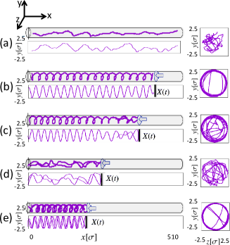
Upon being compressed, the chain changes its configuration from a random deflection to a helix; a snapshot at $X(t)=414\sigma$ is shown in Fig. 1(b). Further compression causes one of the chain ends to turn around as in Fig. 1 (c). This entails rapid decrease in the pressure at both of the walls, as the helix relaxes. The kink, i.e. turning point, moves to the middle of the chain as the piston moves, and the chain becomes doubly folded as in Fig. 1 (d). At a higher compression, the double-fold chain transforms to a double-fold helix as shown in Fig.1 (e). Eventually, the double helix turns around once more and relaxes as the single helix does.

Figure 2(a) shows the change in polymer configuration upon compression; the $y$-coordinate of bead positions $y_{i}(t)$ are plotted in the gray scale for the bead number $i$ on the vertical axis and the distance between the walls $X(t)$ on the horizontal axis. Note that the initial randomly deflected configuration is represented along the vertical line at the right end of the plot at $X=510\sigma$, and the system moves towards left as being compressed. The randomly blurred patterns in the plot correspond to the random deflection. Around $X(t)=X_{c}\simeq 488\sigma$ the helix structure is formed as can be seen from the zebra pattern. It should be noted that $X_{c}\simeq\langle L_{x}\rangle$, i.e., the helix transition takes place under the minute influence of the piston. We will discuss this later.

As $X(t)$ decreases further, the pitch of the helix becomes shorter. At $X(t)=X_{d}\simeq 365\sigma$ in Fig. 2(a), the right end of the chain turns around and the helix structure vanishes as the chain relaxes. The sharp line appearing in the blur region for $X_{c2}<X<X_{d}$ shows the bead number where the chain turns around. One can see that the kink appears at $X=X_{d}$ near the end of the chain, then it moves towards the middle of the chain. At $X(t)=X_{c2}\simeq 245\sigma$, a double-fold helix is formed, whose pitch decreases upon further compression.

Figure 2: (a) Kymographic representation of the chain configuration characterized by the sequence of $y$ coordinate of beads. Horizontal and vertical axes specify the channel length $X$ and the bead index $i$, respectively, The $y$ -coordinate is shown in the gray scale. (b) Average bending energy per bending angle as a function of $X$. The dashed line represents the analytic expression for noise-free structure given in Eq. (7).

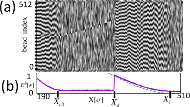
The bending energy $E^{b}=\frac{1}{N-2}\sum_{i=2}^{N-1}U^{b}_{i}$ is shown in Fig. 2(b). As the chain is compressed, $E^{b}$ increases, but decreases discontinuously at $X(t)=X_{d}$ when one of the chain ends turns around, because the helix relaxes into the double-fold random deflection state. In the region $X_{c2}<X(t)<X_{d}$ the bending energy $E^{b}$ stays low and starts to increase again when the double-fold helix is formed.

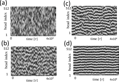
Fig. 3 shows the spatio-temporal structural patterns with the channel length $X$ being fixed at some values near $X_{c}$. Unlike Fig. 2(a), the horizontal axis in Fig. 3 is time, so that the time course of the fluctuating structures near the onset of helix formation are clearly visible. In Fig. 3(a) at $X=498\sigma>\langle L_{x}\rangle=487.45\sigma$, one only sees a disordered pattern, which corresponds to the configuration of an uncompressed confined polymer spreading along the cylinder axis (Fig.1(a)). In Fig. 3(b) at $X=483\sigma<X_{c}\simeq 488\sigma$, a highly fluctuating but characteristic zebra structure is visible, indicating that the chain has helical turns, which are created and annihilated temporally. With further compression, the fluctuating helical structures become more stable at $X=475\sigma$ in Fig. 3(c), and the helix structure establishes through the whole chain at $X=467\sigma$ in Fig. 3(d).

Figure 3: Kymographic representation of the spatio-temporal configurations of the chain at $X=498\sigma$ (a), $483\sigma$ (b), $475\sigma$ (c), and $467\sigma$ (d). The $y$ co-ordinate is shown in the gray scale.

IV discussion

The characteristic force of the helix formation could be addressed through the derivative of the bending energy, i.e., $f_{c}=L_{0}|dE^{b}(X)/dX|_{X=X_{c}}$ at the transition point. To evaluate it, we consider the helix configuration without thermal noise, which is represented as

$${\mbox{\boldmath$r$}}_{\natural}(s)=\left(\frac{ps}{\pi D}\sin{\phi},\frac{D}{2}\cos{\theta(s)},\frac{D}{2}\sin{\theta(s)}\right)$$ (6)

with the arc length $s\in(0,L_{0})$, where the subscript ($\natural$) indicates the quantity without noise. Here the angle $\phi$ is related to the helix pitch $p$ through $\tan{\phi}=\pi D/p$, and $\theta(s)=2s\sin{\phi}/D$ is the angle in the cross-sectional circle. Noting the axial length of the helix $X=L_{0}\cos{\phi}$, the bending energy of the structure is calculated as

$$E^{b}_{\natural}(X)=\frac{\kappa}{2L_{0}}\int^{L_{0}}_{0}ds\left(\frac{d^{2}\bm{r}_{\natural}(s)}{ds^{2}}\right)^{2}=\frac{2\kappa}{D^{2}}\left[1-\left(\frac{X}{L_{0}}\right)^{2}\right]^{2}$$ (7)

From this and using the relation $X_{c}\simeq\langle L_{x}\rangle$ given in Eq. (5), we find

$$f_{c\natural}\approx 16\alpha_{0}{\kappa\over\lambda^{2}},$$ (8)

where $\lambda=l_{p}^{1/3}D^{2/3}$ is the deflection length Odijk (1983). Apart from a numerical constant $16\alpha_{0}\simeq 2.7$, this expression coincides with the buckling force of the filament with the bending rigidity $\kappa$ and the length $\lambda$ Landau and Lifshitz (1986). Our analysis thus identifies the helix formation as the buckling of the deflection segment.

In reality, the helix is substantially disturbed by the thermal noise, in particular, close to the transition point. We thus analyze the spatial correlation near the onset of the helix formation $X\simeq X_{c}$ by the orientational correlation function

$$C_{b}(|i-j|)=\langle\mbox{\boldmath$t$}^{\perp}_{i}(t)\cdot\mbox{\boldmath$t$}^{\perp}_{j}(t)\rangle,$$ (9)

where $\mbox{\boldmath$t$}_{i}^{\perp}$ is the transverse component of the tangent vector $\mbox{\boldmath$t$}_{i}(t)\equiv(\mbox{\boldmath$r$}_{i+1}-\mbox{\boldmath$r$}_{i})/|\mbox{\boldmath$r$}_{i+1}-\mbox{\boldmath$r$}_{i}|\equiv\mbox{\boldmath$t$}^{x}_{i}(t)+\mbox{\boldmath$t$}^{\perp}_{i}(t)$. For the uncompressed state, one can evaluate the correlation function analytically by the effective free energy Köster et al. (2005); Wagner et al. (2007); Wang and Gao (2007)

$$F=\frac{\kappa}{2}\int^{L_{0}}_{0}ds\left(\frac{d^{2}\bm{r}(s)}{ds^{2}}\right)^{2}+\frac{k}{2}\int^{L_{0}}_{0}ds(\bm{r}^{\perp}(s))^{2},$$ (10)

where the fluctuating chain configuration is represented as ${\mbox{\boldmath$r$}}(s)$ with the arc length $s\in(0,L_{0})$ so that the tangent vector is given by ${\mbox{\boldmath$t$}}(s)=d{\mbox{\boldmath$r$}}(s)/ds$. The confinement effect is modeled by the harmonic potential with the spring constant per unit length $k$. The excluded-volume effect can be safely neglected in Odijk regime $D/l_{p}\ll 1$, where small fluctuations around the straight configuration can be analyzed by the Gaussian approximation, leading to

$$\langle{\mbox{\boldmath$t$}}^{\perp}(s)\cdot{\mbox{\boldmath$t$}}^{\perp}(0)\rangle=\frac{2}{L_{0}}\frac{k_{B}T}{\kappa}\sum_{q_{n}}\frac{q_{n}^{2}}{q_{n}^{4}+k/\kappa}e^{-iq_{n}s}$$ (11)

with the wave number $q_{n}=2\pi n/L_{0}$. Approximating the summation in Eq. (11) by the integral, we obtain

$$\langle{\mbox{\boldmath$t$}}^{\perp}(s)\cdot{\mbox{\boldmath$t$}}^{\perp}(0)\rangle=\frac{\lambda}{\sqrt{2}l_{p}}\cos\left(\frac{s}{\lambda}+\frac{\pi}{4}\right)\exp\left(-\frac{s}{\lambda}\right),$$ (12)

where the deflection length $\lambda=l_{p}^{1/3}D^{2/3}=(4\kappa/k)^{1/4}$ naturally appears from the requirement that the chain is confined in a cylinder with diameter $D$, i.e., $\langle|{\mbox{\boldmath$r$}}^{\perp}(s)|^{2}\rangle=(D/2)^{2}$.

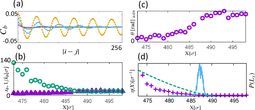
Fig. 4(a) shows the correlation function $C_{b}(|i-j|)$ obtained by simulations for various channel lengths $X$. The functions are well fitted to the formula

$$C_{b}(|i-j|)=A_{b}\cos(k_{b}|i-j|+\theta)\exp(-|i-j|/x_{b}).$$

The fitting parameters are shown in Fig. 4(b) and (c) in the vicinity of $X=X_{c}$. For large $X$, $x_{b}$ and $k_{b}$ are almost the same and nearly constant $x_{b}\simeq 1/k_{b}\simeq 20\sigma$ in agreement with the theoretical estimate by Eq. (12), which gives $\lambda\simeq 23\sigma$ for $D=5\sigma$ and $l_{p}=500\sigma$. The deviation from this at $X<X_{c}$ should be the compression effect. Upon decreasing $X$ below $X_{c}$, the pitch of the helix $1/k_{b}$ decreases while the correlation length $x_{b}$ increases rather rapidly, which means that the helix structure prevails. The phase shift $\theta$ in Fig. 4(d) takes $\theta=\pi/4$ in the large $X$ limit, which is consistent with Eq.  (12). Under compression, $\theta$ decreases toward $\theta=0$.

We introduce the helical oder parameter $\eta$ defined by

$$\eta=\frac{1}{\sigma}\langle{\mbox{\boldmath$t$}}^{\perp}_{i}\times{\mbox{\boldmath$t$}}^{\perp}_{i+1}\rangle$$ (13)

which becomes large for the helical structure. If there is no thermal fluctuation, one can again use Eq. (6) to calculate the helical order parameter

$$\eta_{\natural}(X)=\frac{2}{D}\left(\frac{L^{2}-X^{2}}{L^{2}}\right)^{\frac{3}{2}}\approx\frac{2}{D}\left(2\frac{L-X}{L}\right)^{\frac{3}{2}}.$$ (14)

In Fig. 4(d), we shows the helical order parameter obtained by the numerical simulation along with the analytical expression (14) for the case without fluctuation. The oder parameter $\eta$ of the numerical results starts to grow at $X\simeq X_{c}$. The chain seems to form the helix right at the onset of compression with no appreciable weak compression regime without any structural change. Upon further compression, the oder parameter reaches to the value for the no thermal fluctuation case. To resolve the onset point more carefully, we overlay in Fig. 4(d) the distribution of the chain extension $L_{x}$ without the compression, from which the width $\sqrt{(\delta L_{x})^{2}}\simeq 0.516\sigma$ is extracted. A careful inspection of Figs. 4(a)-(d) shows $X_{c}\simeq\langle L_{x}\rangle$, thus, the chain feels the compression force and starts to form a helix when the channel length reaches the average chain extension in the channel.

Such a feature of the compressive response, i.e., sudden buckling into helix without a notable sign of ordinary linear response regime, could be understood in the following way. The fluctuation of $L_{x}$ has been estimated as

$$\langle(\delta L_{x})^{2}\rangle=\beta_{0}\frac{D^{2}}{l_{p}}L_{0}=\beta_{0}\frac{\lambda^{3}}{l_{p}^{2}}L_{0}$$ (15)

with $\beta_{0}\simeq 0.00754$ for the circular channel Burkhardt et al. (2010). The standard deviation by this expression $\sqrt{\langle(\delta L_{x})^{2}\rangle}=0.43\sigma$ is in agreement with $0.516\sigma$ by the numerical simulation . If we estimate the spring constant as

$$k_{\parallel}=\frac{k_{B}T}{\langle(\delta L_{x})^{2}\rangle},$$ (16)

the typical force $f^{*}$ in the linear response regime should be

$$f^{*}\simeq k_{\parallel}\sqrt{\langle(\delta L_{x})^{2}\rangle}=\frac{k_{B}T}{\sqrt{\langle(\delta L_{x})^{2}\rangle}}.$$ (17)

On the other hand, as we already discussed, the critical force $f_{c}$ to induce the helix transition is identified as the buckling force of the deflection segment as given by Eq. (8).

In order for the weak compression regime to exist, we would expect $f^{*}<f_{c}$, but this condition leads to

$$L_{0}\ >\ L_{0}^{\rm th}\equiv{\lambda\over(16\alpha_{0})^{2}\beta_{0}}\approx{\lambda\over 0.055}.$$ (18)

In other words, the polymer with $L_{0}$ shorter than $L_{0}^{\rm th}$ will transform into helix by the compression weaker than that by the thermal fluctuation. Because $\beta_{0}$ is very small, $L_{0}^{\rm th}$ could be quite large; for our chain with $\lambda\simeq 23\sigma$, $L_{0}^{th}\simeq 420\sigma$, already comparable to the chain length $L_{0}\simeq 491\sigma$ used in our simulation  . In principle, the compressive mode of a long chain is very soft (cf. $L_{0}^{-1}$ factor in the spring constant). However, the smallness of $\beta_{0}$ makes the stiffness relatively high for practical chains with moderate length. This stiffening facilitates rigid response to the compressive force, in which the deflection segment buckles into the helix.

Figure 4: (a) The bond correlation function $C_{b}$ is plotted in the vicinity of $X_{c}$ for $X=500\sigma$ ($\circ$), $485\sigma$ ($\blacktriangle$), $477\sigma$ ($\blacksquare$), and $469\sigma$ ($\bullet$) with $l_{p}=500$. (b)Characteristic decay lengths $x_{b}$ ($\circ$) and inverse wave number $1/k_{b}$ ($\blacktriangle$) of the bond correlation function as a function of $X$. (c) Phase sift $\theta$ in the bond correlation function as a function of $X$. (d) Helical order parameter $\eta$ as a function of $X$: the numerical results (+) and the analytical expression (14) without thermal noise (broken line). The probability distribution $P$ of the projected chain length $L_{x}$ without compression is overlaid with the common $x$ axis (blue line).

We have checked that the scenario described above is robust against the change in the persistence length. For chains with $l_{p}/\sigma=250,\ 100$, the helix formation at $X_{c}$ and its collapse into the double-fold at $X_{d}$ are clearly seen, albeit with the shift of the critical values $X_{c}$ and $X_{d}$. For chains with $l_{p}/\sigma=50$, the helical structure in the snapshot is not easily recognizable by the naked eye; the chain is transformed into the double-fold before the clear helix is formed. But the analysis of the spatial correlation $C_{b}$ and the order parameter $\eta$ indicates the departure from the disordered structure in a certain range of $X$, hinting the local and transient helix. Overall, with the decrease in $l_{p}/D$, the interval for the helix state $X_{c}-X_{d}$ decreases, and it is expected that such an interval would eventually disappear for sufficiently small $l_{p}/D$. Our simulation indicates the threshold $(l_{p}/D)_{th}\sim 10$ i.e. $(\lambda/D)_{th}=(l_{p}/D)^{1/3}\sim 2$. We do not understand yet the mechanism of helix instability at $X=X_{d}$.

If we move the end cap backward after the double-fold state ($X_{c2}<X<X_{d}$) is formed, the helix never forms again, but the uncompressed state is reached directly. This hysteresis is easy to understand by comparing the bending energies between the helix and the double-fold states under compression. While the bending energy of the helix increases under compression, that of the double-fold random deflection state is constant as long as a turing point exists. In the case of $l_{p}/D\gg(l_{p}/D)_{th}$, the compression of the initially unperturbed chain always leads to the formation of helical structure because the bending energy of nascent helix is lower than that of the double-fold random deflection state. The helix, once formed, is very stable, because turning around a chain end gets more unlikely for larger $l_{p}/D$ due to higher energetic penalty of bending.

In order to examine experimental relevance of the phenomenon, let us discuss some of the system parameters. Most of our simulations are performed using a polymer with its persistent length $l_{p}=500\sigma$ pushed into the cylinder of the diameter $D=5\sigma$, but we also performed some simulations with $l_{P}=100\sigma$ and $50\sigma$ and observed the helix formation. If we use a DNA of $l_{p}\sim 50$ nm, a nanochannel diameter of $D=5\sigma$ corresponds to $D=0.5\sim 5$ nm. In the case of stiffer polymer such as actin filament, for which $l_{P}\sim 16\ {\rm\mu}$ m, the cylinder diameter can be as large as sub-micron range, which should be realistic experimentally. The critical force of compression $f_{c}$ given by Eq. (8) for the helix formation is of the order of pN for the actin filament compressed in the cylinder of the diameter $D\sim 100$ nm, where the deflection length $\lambda\sim 500$ nm.

The experimental set up for nano-piston has been proposed in ref.[17,18], where the nano-piston is controlled by an optically trapped bead. Another possibility may be AFM, in which case the size of the bead is not limited by the wave length of the laser. We expect that the present process is experimentally accessible through the hysteresis in the relation between the displacement of the piston and the compression force during compression and extension.

V conclusion

In summary, we have reported the formation of helical structure of semiflexible polymer in a nanochannel subjected to the longitudinal compressive force. This would provide an interesting possibility to control the structure of various semiflexible polymer under confinement. In the present report, we have analyzed the initial response, and have pointed out the peculiarity of the compressive response of semiflexible polymer; the phenomenon is most naturally interpreted as the buckling of deflection segment, and the structural transition to the helix takes place even at the very weak compression by the confinement length $X$ comparable to $\left<L_{x}\right>$. This means the intermittent force at the cap by the thermal fluctuation can induce the helix structure.