Classification and Representation via Separable Subspaces: Performance Limits and Algorithms

Ishan Jindal, Student Member, IEEE and Matthew Nokleby, Member, IEEE
Department of Electrical and Computer Engineering, Wayne State University, Detroit, MI, 48202, USA
Email: {ishan.jindal, matthew.nokleby}@wayne.edu
Abstract

We study the classification performance of Kronecker-structured models in two asymptotic regimes and developed an algorithm for separable, fast and compact K-S dictionary learning for better classification and representation of multidimensional signals by exploiting the structure in the signal. First, we study the classification performance in terms of diversity order and pairwise geometry of the subspaces. We derive an exact expression for the diversity order as a function of the signal and subspace dimensions of a K-S model. Next, we study the classification capacity, the maximum rate at which the number of classes can grow as the signal dimension goes to infinity. Then we describe a fast algorithm for Kronecker-Structured Learning of Discriminative Dictionaries (K-SLD2). Finally, we evaluate the empirical classification performance of K-S models for the synthetic data, showing that they agree with the diversity order analysis. We also evaluate the performance of K-SLD2 on synthetic and real-world datasets showing that the K-SLD2 balances compact signal representation and good classification performance.

Index Terms:
Machine learning, subspace models, Kronecker-structured models, Gaussian mixture models, matrix normal distribution, diversity order, classification capacity, principal angles, discriminative K-S dictionary learning.

I Introduction

The classification of high-dimensional signals arises in a variety of image processing settiings: object and digit recognition [1, 2], speaker identification [3, 4], tumor classification [5, 6], and more. A standard technique is to find a low-dimensional representation of the signal, such as a subspace or union of subspaces on which the signal approximately lies. However, for many signals, such as dynamic scene videos [7] or tomographic images [8], the signal inherently is multi-dimensional, involving dimensions of space and/or time. To use standard techniques, one vectorizes the signal, which throws out the spatial structure of the data which could be leveraged to improve representation fidelity, reconstruction error, or classification performance.

In order to exploit multi-dimensional signal structure, researchers have proposed tensor-based dictionary learning techniques, in which the signal of interest is a matrix or a higher-order tensor and the dictionary defining the (union of) subspace model is a tensor. A simple tensor-based model is the Kronecker-structured (K-S) model, in which a two-dimensional signal is represented by a coefficient matrix and two matrix dictionaries that pre- and post-multiply the coefficient matrix, respectively. Vectorizing this model leads to a dictionary that is the Kronecker product of two smaller dictionaries; hence the K-S model is a specialization of subspace models. This model is applied to spatio-temporal data in [9], low-complexity methods for estimating K-S covariance matrices are developed in [10], and it is shown that the sample complexity of K-S models is smaller than standard union-of-subspace models in [11].

As standard union-of-subspace models have proven successful for classification tasks [12, 13, 14], a natural question is the classification performance of K-S subspace models. In this paper, we address this question from an information-theoretic perspective and developed an algorithm for learning discriminative K-S dictionaries. We consider a signal model in which each signal class is associated with a subspace whose basis is the Kronecker product of two smaller dictionaries; equivalently, we suppose that each signal class has a matrix normal distribution, where the row and column covariances are approximately low rank. Here the covariance of signal class follows a specific structure which is exactly the Kronecker product of two lower dimensional covariance matrices [15, 16, 17]. In this sense, signals are drawn from a matrix Gaussian mixture model (GMM), similar to [18], where each K-S subspace is associated with a mixture component.

To find the underlying low dimensional representation of signals, dictionary learning methods are widely used [19, 20, 21]. The underlying signal is compactly represented by a few large coefficients in an overcomplete dictionary. In a standard dictionary learning setting a 1-D signal yisubscript𝑦𝑖y_{i} is represented using a sparse coefficient vector xisubscript𝑥𝑖x_{i}, where an overcomplete dictionary Disubscript𝐷𝑖D_{i} is learned by minimization problems similar to

argmin{Di,xi}iyiDixiF2+λxi1subscriptsubscript𝐷𝑖subscript𝑥𝑖subscript𝑖superscriptsubscriptnormsubscript𝑦𝑖subscript𝐷𝑖subscript𝑥𝑖𝐹2𝜆subscriptnormsubscript𝑥𝑖1\arg\,\min_{\{D_{i},x_{i}\}}\sum_{i}||y_{i}-D_{i}x_{i}||_{F}^{2}+\lambda||x_{i}||_{1} (1)

Where ||||F||\cdot||_{F} denotes the Forbenius norm, ||||1||\cdot||_{1} denotes the l1subscript𝑙1l_{1}-norm, and λ𝜆\lambda denotes the strength of the sparsity prior. Well-established methods for dictionary learning in this framework include K-SVD [22] and the method of optimal directions [23]. These methods are targeted at dictionaries that faithfully represent the signal, and do not specifically consider classification.

Methods for incorporating discriminative ability into dictionary learning have been proposed, such as discriminative K-SVD [12] (D-KSVD) and label consistent (LC-KSVD) [24], which jointly learn a linear classifier and an overcomplete dictionary that is shared in common among the classes. Signals are then classified in the feature space induced by the dictionary. By contrast, [25, 13, 26, 27] propose methods for learning class-specific dictionaries, either by promoting incoherence among dictionaries or learning class-specific features. Signals are then classified by choosing the dictionary that minimizes the reconstruction error.

The above methods consider one-dimensional signals; multidimensional signals must first be vectorized, which may sacrifice structural information about the signal that could improve signal representation or classification. To preserve signal structure,[28] extends K-SVD to tensor dictionaries, and [29, 30, 31, 6] employ a variety of tensor decompositions to learn dictionaries tailored to multidimensional structure. These methods boast improved performance over traditional methods on a variety of signal processing tasks, including image reconstruction, image denoising and inpainting, video denoising, and speaker classification.

Similar to [32], we first study the classification performance limits of K-S models in terms of diversity order and classification capacity, characterizing the performance in the limit of high SNR and large signal dimension, respectively. Further, we derive a tight upper bound on the misclassification probability in terms of the pairwise geometry of individual row and column subspaces. Where row and column subspaces correspond to two matrix dictionaries that pre- and post-multiply the coefficient matrix, respectively. We use principal angles between the subspaces as a measure to describe the geometry of subspaces [33, 34].

Finally, to learn discriminative dictionaries, we propose a new method, termed Kronecker-Structured Learning of Discriminative Dictionaries (K-SLD2), that exploit multidimensional structure of the signal. K-SLD2 learns two subspace dictionaries per class: one to represent the columns of the signal, and one to represent the rows. Inspired by [26], we choose dictionaries that both represent each class individually and can be concatenated to form an overcomplete dictionary to represent signals generally. K-SLD2 is fast and learns compact data models with many fewer parameters than standard dictionary learning methods. We evaluate the performance of K-SLD2 on the Extended YaleB and UCI EEG database. The resulting dictionaries improve classification performance by up to 5% when training sets are small, improve reconstruction performance across the board, and result in dictionaries with no more than 5% of the storage requirements of existing subspace models.

In Section II, we describe the K-S classification model in detail. In Section III we derive the diversity order for K-S classification problems, showing the exponent of the probability of error as the SNR goes to infinity. This analysis depends on a novel expression, presented in Lemma 3, for the rank of sums of Kronecker products of tall matrices. In Section IV we provide high-SNR approximations to the classification capacity. In Section V, we propose a discriminative K-S dictionary learning algorithm which balances the learning of class-specific, Kronecker-structured subspaces against the learning of an general overcomplete dictionary that allows for the representation of general signals. In Section VI we show that the empirical classification performance of K-S models agrees with the diversity analysis and evaluate the performance of proposed discriminative algorithm on extended YaleB face recognition dataset and EEG signal dataset correlating the EEG signals with individual’s alcoholism.

II Problem Definition

II-A Kronecker-structured Signal Model

To formalize the classification problem, let the signal of interest 𝐘m1×m2𝐘superscriptsubscript𝑚1subscript𝑚2\mathbf{Y}\in\mathbb{R}^{m_{1}\times m_{2}} be a matrix whose entries are distributed according to one of L𝐿L class-conditional densities pl(𝐘)subscript𝑝𝑙𝐘p_{l}(\mathbf{Y}). Each class-conditional density corresponds to a Kronecker-structured model described by the pair of matrices 𝐀lm1×n1subscript𝐀𝑙superscriptsubscript𝑚1subscript𝑛1\mathbf{A}_{l}\in\mathbb{R}^{m_{1}\times n_{1}} and 𝐁lm2×n2subscript𝐁𝑙superscriptsubscript𝑚2subscript𝑛2\mathbf{B}_{l}\in\mathbb{R}^{m_{2}\times n_{2}}. The matrix 𝐀lsubscript𝐀𝑙\mathbf{A}_{l} describes the subspace on which the columns of 𝐘𝐘\mathbf{Y} approximately lie, and 𝐁lsubscript𝐁𝑙\mathbf{B}_{l} describes the subspace on which the rows of 𝐘𝐘\mathbf{Y} approximately lie. More precisely, if 𝐘𝐘\mathbf{Y} belongs to class l𝑙l, it has the form

𝐘=𝐀l𝐗𝐁lT+𝐙,𝐘subscript𝐀𝑙superscriptsubscript𝐗𝐁𝑙𝑇𝐙\mathbf{Y}=\mathbf{A}_{l}\mathbf{X}\mathbf{B}_{l}^{T}+\mathbf{Z}, (2)

where 𝐙m1×m2𝐙superscriptsubscript𝑚1subscript𝑚2\mathbf{Z}\in\mathbb{R}^{m_{1}\times m_{2}} has i.i.d. zero-mean Gaussian entries with variance σ2>0superscript𝜎20\sigma^{2}>0, and 𝐗n1×n2𝐗superscriptsubscript𝑛1subscript𝑛2\mathbf{X}\in\mathbb{R}^{n_{1}\times n_{2}} has i.i.d. zero-mean Gaussian entries with unit variance. We can also express 𝐘𝐘\mathbf{Y} in vectorized form:

𝐲=(𝐁l𝐀l)𝐱+𝐳,𝐲tensor-productsubscript𝐁𝑙subscript𝐀𝑙𝐱𝐳\mathbf{y}=(\mathbf{B}_{l}\otimes\mathbf{A}_{l})\mathbf{x}+\mathbf{z}, (3)

for coefficient vector 𝐱=vec(𝐗)N𝐱vec𝐗superscript𝑁\mathbf{x}=\mathrm{vec}(\mathbf{X})\,\in\mathbb{R}^{N}, and noise vector 𝐳M𝐳superscript𝑀\mathbf{z}\in\mathbb{R}^{M}, where N=n1n2𝑁subscript𝑛1subscript𝑛2N=n_{1}n_{2}, M=m1m2𝑀subscript𝑚1subscript𝑚2M=m_{1}m_{2}, and where tensor-product\otimes is the usual Kronecker product. Then, the class-conditional density of 𝐲𝐲\mathbf{y} is

pl(𝐲)=𝒩(0,(𝐁l𝐀l)(𝐁𝐥𝐀𝐥)T+σ2𝐈).subscript𝑝𝑙𝐲𝒩0tensor-productsubscript𝐁𝑙subscript𝐀𝑙superscripttensor-productsubscript𝐁𝐥subscript𝐀𝐥𝑇superscript𝜎2𝐈p_{l}(\mathbf{y})=\mathcal{N}(0,(\mathbf{B}_{l}\otimes\mathbf{A}_{l})(\mathbf{B_{l}}\otimes\mathbf{A_{l}})^{T}+\sigma^{2}\cdot\mathbf{I}). (4)

In other words, the vectorized signal 𝐲𝐲\mathbf{y} lies near a subspace with a Kronecker structure that encodes the row and column subspaces of 𝐘𝐘\mathbf{Y}.

In the sequel, we will characterize the performance limits over ensembles of classification problems of this form. To this end, we parameterize the set of class-conditional densities via

𝒜(m1,m2,n1,n2)=m1×n1×m2×n2,𝒜subscript𝑚1subscript𝑚2subscript𝑛1subscript𝑛2superscriptsubscript𝑚1subscript𝑛1superscriptsubscript𝑚2subscript𝑛2\mathcal{A}(m_{1},m_{2},n_{1},n_{2})=\mathbb{R}^{m_{1}\times n_{1}}\times\mathbb{R}^{m_{2}\times n_{2}}, (5)

which contains the set of matrices indicating the row and column subspaces given signal and subspace dimensions m1,m2,n1,n2subscript𝑚1subscript𝑚2subscript𝑛1subscript𝑛2m_{1},m_{2},n_{1},n_{2}. We can represent an L𝐿L-ary classification problem by a tuple 𝐚=(a1,,aL)𝒜L(m1,m2,n1,n2)𝐚subscript𝑎1subscript𝑎𝐿superscript𝒜𝐿subscript𝑚1subscript𝑚2subscript𝑛1subscript𝑛2\mathbf{a}=(a_{1},\cdots,a_{L})\in\mathcal{A}^{L}(m_{1},m_{2},n_{1},n_{2}), where each al𝒜(m1,m2,n1,n2)subscript𝑎𝑙𝒜subscript𝑚1subscript𝑚2subscript𝑛1subscript𝑛2a_{l}\in\mathcal{A}(m_{1},m_{2},n_{1},n_{2}) is the pair of matrices ai=(𝐀l,𝐁l)subscript𝑎𝑖subscript𝐀𝑙subscript𝐁𝑙a_{i}=(\mathbf{A}_{l},\mathbf{B}_{l}). Let p(𝐲|al)=p(𝐲|𝐀l,𝐁l)=pl(𝐲)𝑝conditional𝐲subscript𝑎𝑙𝑝conditional𝐲subscript𝐀𝑙subscript𝐁𝑙subscript𝑝𝑙𝐲p(\mathbf{y}|a_{l})=p(\mathbf{y}|\mathbf{A}_{l},\mathbf{B}_{l})=p_{l}(\mathbf{y}), for 1lL1𝑙𝐿1\leq l\leq L, denote the class conditional densities parametrized by 𝐚𝒜(m1,m2,n1,n2)𝐚𝒜subscript𝑚1subscript𝑚2subscript𝑛1subscript𝑛2\mathbf{a}\in\mathcal{A}(m_{1},m_{2},n_{1},n_{2}). For a classification problem defined by 𝐚𝐚\mathbf{a}, we can define the average misclassification probability:

Pe(𝐚)=1Ll=1LPr(l^l|𝐲p(𝐲|al),P_{e}(\mathbf{a})=\frac{1}{L}\sum_{l=1}^{L}\Pr(\hat{l}\neq l|\mathbf{y}\sim p(\mathbf{y}|a_{l}), (6)

where l^^𝑙\hat{l} is the output of the maximum-likelihood classifier over the class-conditional densities described by 𝐚lsubscript𝐚𝑙\mathbf{a}_{l}. In this paper, we provide two asymptotic analyses of Pe(𝐚)subscript𝑃𝑒𝐚P_{e}(\mathbf{a}). First, we consider the diversity order, which characterizes the slope of Pe(𝐚)subscript𝑃𝑒𝐚P_{e}(\mathbf{a}) for a particular 𝐚𝐚\mathbf{a} as σ20superscript𝜎20\sigma^{2}\to 0. Second, we consider the classification capacity, which characterizes the asymptotic error performance averaged over 𝐚𝐚\mathbf{a} as n1,m1,n2,m2subscript𝑛1subscript𝑚1subscript𝑛2subscript𝑚2n_{1},m_{1},n_{2},m_{2} go to infinity. For the latter case, we define a prior distribution over the matrix pairs (𝐀l,𝐁l)subscript𝐀𝑙subscript𝐁𝑙(\mathbf{A}_{l},\mathbf{B}_{l}) in each class:

p(𝐚)=p=1m1q=1n1r=1m2s=1n2𝒩(apq;0,1/n1)𝒩(brs;0,1/n2)𝑝𝐚superscriptsubscriptproduct𝑝1subscript𝑚1superscriptsubscriptproduct𝑞1subscript𝑛1superscriptsubscriptproduct𝑟1subscript𝑚2superscriptsubscriptproduct𝑠1subscript𝑛2𝒩subscript𝑎𝑝𝑞01subscript𝑛1𝒩subscript𝑏𝑟𝑠01subscript𝑛2p(\mathbf{a})=\prod_{p=1}^{m_{1}}\prod_{q=1}^{n_{1}}\prod_{r=1}^{m_{2}}\prod_{s=1}^{n_{2}}\mathcal{N}(a_{pq};0,1/n_{1})\cdot\mathcal{N}(b_{rs};0,1/n_{2}) (7)

where apqsubscript𝑎𝑝𝑞a_{pq} is the (p,q)𝑝𝑞(p,q)th element of matrix 𝐀𝐀\mathbf{A} and brssubscript𝑏𝑟𝑠b_{rs} is the (r,s)𝑟𝑠(r,s)th element of matrix 𝐁𝐁\mathbf{B}. Note that the column and row subspaces described by 𝐀𝐀\mathbf{A} and 𝐁𝐁\mathbf{B} are uniformly distributed over the Grassmann manifold because the matrix elements are i.i.d. Gaussian; however, the resulting K-S subspaces are not uniformly distributed.

II-B Diversity Order

For a fixed classification problem 𝐚𝐚\mathbf{a}, the diversity order characterizes the decay of the misclassification probability as the noise power goes to zero. By analogy with the definition of the diversity order in wireless communications [35], we consider the asymptotic slope of Pe(𝐚)subscript𝑃𝑒𝐚P_{e}(\mathbf{a}) on a logarithmic scale as σ20superscript𝜎20\sigma^{2}\to 0 that is the mismatch between data and model is vanishingly small. Formally, the diversity order is defined as

d(𝐚)=limσ20logPe(𝐚)12log(1/σ2).𝑑𝐚subscriptsuperscript𝜎20subscript𝑃𝑒𝐚121superscript𝜎2d(\mathbf{a})=\lim_{\sigma^{2}\rightarrow 0}-\frac{\log P_{e}(\mathbf{a})}{\frac{1}{2}\log(1/\sigma^{2})}. (8)

In Section III, we characterize exactly the diversity order for almost every 𝐚𝐚\mathbf{a}.

II-C Classification Capacity

The classification capacity characterizes the number of unique subspaces that can be discerned as n1subscript𝑛1n_{1}, n2subscript𝑛2n_{2}, m1subscript𝑚1m_{1} and m2subscript𝑚2m_{2} go to infinity. That is, we derive bounds on how fast the number of classes L𝐿L can grow as a function of signal dimension while ensuring the misclassification probability decays to zero almost surely. Here, we define a variable m𝑚m111Note that m𝑚m is different from M𝑀M, where m𝑚m is the variable we let to go to infinity and M=m1m2𝑀subscript𝑚1subscript𝑚2M=m_{1}m_{2}. and let it go to infinity. As m𝑚m grows to infinity we let the dimensions m1subscript𝑚1m_{1}, m2subscript𝑚2m_{2}, n1subscript𝑛1n_{1} and n2subscript𝑛2n_{2} scale linearly with m𝑚m as follows:

m1(m)=κ1m,m2(m)=κ2m,n1(m)=υ1m,n2(m)=υ2mformulae-sequencesubscript𝑚1𝑚subscript𝜅1𝑚formulae-sequencesubscript𝑚2𝑚subscript𝜅2𝑚formulae-sequencesubscript𝑛1𝑚subscript𝜐1𝑚subscript𝑛2𝑚subscript𝜐2𝑚m_{1}(m)=\lfloor\kappa_{1}m\rfloor,\,m_{2}(m)=\lfloor\kappa_{2}m\rfloor,\\ n_{1}(m)=\lfloor\upsilon_{1}m\rfloor,n_{2}(m)=\lfloor\upsilon_{2}m\rfloor (9)

for υ1,υ21subscript𝜐1subscript𝜐21\upsilon_{1},\upsilon_{2}\geq 1 and 0κ1,κ21formulae-sequence0subscript𝜅1subscript𝜅210\leq\kappa_{1},\kappa_{2}\leq 1. We let the number of classes L𝐿L grow exponentially in m𝑚m as:

L(m)=2ρm1(m)m2(m),𝐿𝑚superscript2𝜌subscript𝑚1𝑚subscript𝑚2𝑚L(m)=\lfloor 2^{\rho m_{1}(m)m_{2}(m)}\rfloor, (10)

for some ρ0𝜌0\rho\geq 0, which we call the classification rate. We say that the classification rate ρ𝜌\rho is achievable if limmE[Pe(𝐚)]=0subscript𝑚𝐸delimited-[]subscript𝑃𝑒𝐚0\lim_{m\rightarrow\infty}E[P_{e}(\mathbf{a})]=0. For fixed signal dimension ratios υ1,υ2,κ1subscript𝜐1subscript𝜐2subscript𝜅1\upsilon_{1},\upsilon_{2},\kappa_{1} and κ2subscript𝜅2\kappa_{2}, we define C(υ1,υ2,κ1,κ2)𝐶subscript𝜐1subscript𝜐2subscript𝜅1subscript𝜅2C(\upsilon_{1},\upsilon_{2},\kappa_{1},\kappa_{2}) as the supremum over all achievable classification rates, and we call C(υ1,υ2,κ1,κ2)𝐶subscript𝜐1subscript𝜐2subscript𝜅1subscript𝜅2C(\upsilon_{1},\upsilon_{2},\kappa_{1},\kappa_{2}) (sometimes abbreviated by C𝐶C) the classification capacity.

We can bound the classification capacity by the mutual information between the signal vector 𝐲𝐲\mathbf{y} and the matrix pair (𝐀(\mathbf{A}, 𝐁)\mathbf{B}) that characterizes each Kronecker-structured class.

Lemma 1.

The classification capacity satisfies:

ClimmI(𝐲;𝐀,𝐁)m1(m)m2(m)𝐶subscript𝑚𝐼𝐲𝐀𝐁subscript𝑚1𝑚subscript𝑚2𝑚C\leq\lim_{m\rightarrow\infty}\frac{I(\mathbf{y};\mathbf{A},\mathbf{B})}{m_{1}(m)m_{2}(m)} (11)

Where the mutual information is computed with respect to p(𝐚)𝑝𝐚p(\mathbf{a}).

To prove lower bounds on the diversity order and classification capacity, we will need the following lemma, which gives the well-known Bhattacharyya bound on the probability of error of a maximum-likelihood classifier that chooses between two Gaussian hypotheses.

Lemma 2 ([36]).

Consider a signal distributed according to 𝒩(μ1,Σ1)𝒩subscript𝜇1subscriptΣ1\mathcal{N}(\mu_{1},\Sigma_{1}) or 𝒩(μ2,Σ2)𝒩subscript𝜇2subscriptΣ2\mathcal{N}(\mu_{2},\Sigma_{2}) with equal priors. Then, define

b=12ln(|Σ1+Σ22||Σ1|12|Σ2|12)+18(μ1μ2)[Σ1+Σ22]1(μ1μ2)𝑏12subscriptΣ1subscriptΣ22superscriptsubscriptΣ112superscriptsubscriptΣ21218subscript𝜇1subscript𝜇2superscriptdelimited-[]subscriptΣ1subscriptΣ221subscript𝜇1subscript𝜇2b=\frac{1}{2}\ln\left(\frac{|\frac{\Sigma_{1}+\Sigma_{2}}{2}|}{|\Sigma_{1}|^{\frac{1}{2}}|\Sigma_{2}|^{\frac{1}{2}}}\right)+\frac{1}{8}(\mu_{1}-\mu_{2})\left[\frac{\Sigma_{1}+\Sigma_{2}}{2}\right]^{-1}(\mu_{1}-\mu_{2}) (12)

Supposing maximum likelihood classification, the misclassification probability is bounded by

Pe(μ1,Σ1,μ2,Σ2)12exp(b).subscript𝑃𝑒subscript𝜇1subscriptΣ1subscript𝜇2subscriptΣ212𝑏P_{e}(\mu_{1},\Sigma_{1},\mu_{2},\Sigma_{2})\leq\frac{1}{2}\exp(-b). (13)

II-D Subspace Geometry

We characterize the subspace geometry in terms of principal angles. Principal angle defines as the canonical angles between elements of subspaces, and they induce a distance metric on the Grassmann manifold. If the principal angles between subspaces is large, this means that the subspaces are far apart and easily discernible.

Consider two linear subspaces 𝒜1subscript𝒜1\mathcal{A}_{1} and 𝒜2subscript𝒜2\mathcal{A}_{2} of msuperscript𝑚\mathbb{R}^{m} with same dimensions n𝑛n each. The principal angles between these two subspaces are defined recursively as follows:

cos(θt)subscript𝜃𝑡\displaystyle\cos(\theta_{t}) =maxut𝒜1maxvt𝒜2utTvtabsentsubscriptsubscript𝑢𝑡subscript𝒜1subscriptsubscript𝑣𝑡subscript𝒜2superscriptsubscript𝑢𝑡𝑇subscript𝑣𝑡\displaystyle=\max_{u_{t}\in\mathcal{A}_{1}}\max_{v_{t}\in\mathcal{A}_{2}}u_{t}^{T}v_{t}
subject to utTut=1,vtTvt=1,formulae-sequencesubject to superscriptsubscript𝑢𝑡𝑇subscript𝑢𝑡1superscriptsubscript𝑣𝑡𝑇subscript𝑣𝑡1\displaystyle\,\text{subject to }\quad u_{t}^{T}u_{t}=1,\,v_{t}^{T}v_{t}=1,
utTui=0,vtTvt=0,(i<t)formulae-sequencesuperscriptsubscript𝑢𝑡𝑇subscript𝑢𝑖0superscriptsubscript𝑣𝑡𝑇subscript𝑣𝑡0𝑖𝑡\displaystyle\,\,\quad\quad\quad\quad\quad u_{t}^{T}u_{i}=0,\,v_{t}^{T}v_{t}=0,\quad(i<t)

where 0θ1θ2θn1π20subscript𝜃1subscript𝜃2subscript𝜃subscript𝑛1𝜋20\leq\theta_{1}\leq\theta_{2}\leq\cdots\leq\theta_{n_{1}}\leq\frac{\pi}{2} and the first principal angle θ1subscript𝜃1\theta_{1} is the smallest angle between all pairs of unit vectors in the first and the second subspaces [37].

The principal angles can be computed directly via computing the singular value decomposition (SVD) of 𝐀1T𝐀2superscriptsubscript𝐀1𝑇subscript𝐀2\mathbf{A}_{1}^{T}\mathbf{A}_{2}, where 𝐀1subscript𝐀1\mathbf{A}_{1} and 𝐀2subscript𝐀2\mathbf{A}_{2} are orthonormal basis for the subspaces 𝒜1subscript𝒜1\mathcal{A}_{1} and 𝒜2subscript𝒜2\mathcal{A}_{2}, respectively.

𝐀1T𝐀2=𝐔Acos(ΘA)𝐕AT,superscriptsubscript𝐀1𝑇subscript𝐀2subscript𝐔𝐴subscriptΘ𝐴superscriptsubscript𝐕𝐴𝑇\mathbf{A}_{1}^{T}\mathbf{A}_{2}=\mathbf{U}_{A}\cos(\Theta_{A})\mathbf{V}_{A}^{T},

where the cosine of principal angles, cos(ΘA)=diag(cos(θ1A),cos(θ2A),,cos(θn1A))subscriptΘ𝐴diagsuperscriptsubscript𝜃1𝐴superscriptsubscript𝜃2𝐴superscriptsubscript𝜃subscript𝑛1𝐴\cos(\Theta_{A})=\text{diag}(\cos(\theta_{1}^{A}),\cos(\theta_{2}^{A}),\cdots,\cos(\theta_{n_{1}}^{A})), are the singular values of 𝐀1T𝐀2superscriptsubscript𝐀1𝑇subscript𝐀2\mathbf{A}_{1}^{T}\mathbf{A}_{2}.

In this problem, suppose 𝐀1subscript𝐀1\mathbf{A}_{1} and 𝐀2subscript𝐀2\mathbf{A}_{2} are orthonormal basis for the subspaces 𝒜1subscript𝒜1\mathcal{A}_{1} and 𝒜2subscript𝒜2\mathcal{A}_{2} on which columns of signal approximately lies and 𝐁1subscript𝐁1\mathbf{B}_{1} and 𝐁2subscript𝐁2\mathbf{B}_{2} are orthonormal basis for the subspaces 1subscript1\mathcal{B}_{1} and 2subscript2\mathcal{B}_{2} on which rows of signal approximately lies. Then we define the orthonormal basis 𝐃1=𝐁1𝐀1subscript𝐃1tensor-productsubscript𝐁1subscript𝐀1\mathbf{D}_{1}=\mathbf{B}_{1}\otimes\mathbf{A}_{1} and 𝐃2=𝐁2𝐀2subscript𝐃2tensor-productsubscript𝐁2subscript𝐀2\mathbf{D}_{2}=\mathbf{B}_{2}\otimes\mathbf{A}_{2} for the Kronecker-structured subspaces 𝒟1subscript𝒟1\mathcal{D}_{1} and 𝒟2subscript𝒟2\mathcal{D}_{2}, respectively. The cosine of principal angles between 𝐃1subscript𝐃1\mathbf{D}_{1} and 𝐃2subscript𝐃2\mathbf{D}_{2} are the singular values of 𝐃1T𝐃2superscriptsubscript𝐃1𝑇subscript𝐃2\mathbf{D}_{1}^{T}\mathbf{D}_{2} as follows:

𝐃1T𝐃2superscriptsubscript𝐃1𝑇subscript𝐃2\displaystyle\mathbf{D}_{1}^{T}\mathbf{D}_{2} =(𝐁1𝐀1)T(𝐁2𝐀2)absentsuperscripttensor-productsubscript𝐁1subscript𝐀1𝑇tensor-productsubscript𝐁2subscript𝐀2\displaystyle=(\mathbf{B}_{1}\otimes\mathbf{A}_{1})^{T}(\mathbf{B}_{2}\otimes\mathbf{A}_{2})
=(𝐁1T𝐁2)(𝐀1T𝐀2)absenttensor-productsuperscriptsubscript𝐁1𝑇subscript𝐁2superscriptsubscript𝐀1𝑇subscript𝐀2\displaystyle=(\mathbf{B}_{1}^{T}\mathbf{B}_{2})\otimes(\mathbf{A}_{1}^{T}\mathbf{A}_{2})
=(𝐔Bcos(ΘB)𝐕BT)(𝐔Acos(ΘA)𝐕AT)absenttensor-productsubscript𝐔𝐵subscriptΘ𝐵superscriptsubscript𝐕𝐵𝑇subscript𝐔𝐴subscriptΘ𝐴superscriptsubscript𝐕𝐴𝑇\displaystyle=(\mathbf{U}_{B}\cos(\Theta_{B})\mathbf{V}_{B}^{T})\otimes(\mathbf{U}_{A}\cos(\Theta_{A})\mathbf{V}_{A}^{T})
=(𝐔B𝐔A)(cos(ΘB)cos(ΘA))(𝐕B𝐕A)Tabsenttensor-productsubscript𝐔𝐵subscript𝐔𝐴tensor-productsubscriptΘ𝐵subscriptΘ𝐴superscripttensor-productsubscript𝐕𝐵subscript𝐕𝐴𝑇\displaystyle=(\mathbf{U}_{B}\otimes\mathbf{U}_{A})(\cos(\Theta_{B})\otimes\cos(\Theta_{A}))(\mathbf{V}_{B}\otimes\mathbf{V}_{A})^{T}
=𝐔cos(Θ)𝐕T,absent𝐔Θsuperscript𝐕𝑇\displaystyle=\mathbf{U}\cos(\Theta)\mathbf{V}^{T},

where the cosine of principal angle between two Kronecker subspaces is the Kronecker product of cosine of principal angles between two row subspaces and two column subspaces that is cos(Θ)=cos(ΘA)cos(ΘB)Θtensor-productsubscriptΘ𝐴subscriptΘ𝐵\cos(\Theta)=\cos(\Theta_{A})\otimes\cos(\Theta_{B}).

III Diversity Order

As mentioned in Section II, the diversity order measures how quickly misclassification probability decays with the noise power for a fixed number of discernible subspaces. By careful analysis using the Bhattacharrya bound, we derive an exact expression for the diversity order for almost every222With respect to the Lebesgue measure over 𝒜Lsuperscript𝒜𝐿\mathcal{A}^{L}. classification problem. First, we state an expression that holds in general.

Theorem 1.

For a classification problem described by the tuple 𝐚𝒜L𝐚superscript𝒜𝐿\mathbf{a}\in\mathcal{A}^{L} such that r(𝐀l)=n1𝑟subscript𝐀𝑙subscript𝑛1r(\mathbf{A}_{l})=n_{1} and r(𝐁l)=n2𝑟subscript𝐁𝑙subscript𝑛2r(\mathbf{B}_{l})=n_{2} for every l𝑙l, the diversity order is d(𝐚)=rn1n2𝑑𝐚superscript𝑟subscript𝑛1subscript𝑛2d(\mathbf{a})=r^{*}-n_{1}n_{2}, where

r=mini,jr([𝐁i𝐀i𝐁j𝐀j]),superscript𝑟subscript𝑖𝑗𝑟matrixtensor-productsubscript𝐁𝑖subscript𝐀𝑖tensor-productsubscript𝐁𝑗subscript𝐀𝑗r^{*}=\min_{i,j}r(\begin{bmatrix}\mathbf{B}_{i}\otimes\mathbf{A}_{i}&\mathbf{B}_{j}\otimes\mathbf{A}_{j}\end{bmatrix}), (14)

and where r()𝑟r(\cdot) denotes the matrix rank.

Proof:

Applying the Bhattacharyya bound, the probability of a pairwise error between two Kronecker-structured classes i𝑖i and j𝑗j with covariances

Σi=𝐃i𝐃iT+σ2𝐈,Σj=𝐃j𝐃jT+σ2𝐈,formulae-sequencesubscriptΣ𝑖subscript𝐃𝑖superscriptsubscript𝐃𝑖𝑇superscript𝜎2𝐈subscriptΣ𝑗subscript𝐃𝑗superscriptsubscript𝐃𝑗𝑇superscript𝜎2𝐈\Sigma_{i}=\mathbf{D}_{i}\mathbf{D}_{i}^{T}+\sigma^{2}\mathbf{I},\quad\Sigma_{j}=\mathbf{D}_{j}\mathbf{D}_{j}^{T}+\sigma^{2}\mathbf{I},

is bounded by

Pe(𝐃i,𝐃j)12(|𝐃i𝐃iT+𝐃j𝐃jT+2σ2𝐈2||𝐃i𝐃iT+σ2𝐈|12|𝐃j𝐃jT+σ2𝐈|12)12subscript𝑃𝑒subscript𝐃𝑖subscript𝐃𝑗12superscriptsubscript𝐃𝑖superscriptsubscript𝐃𝑖𝑇subscript𝐃𝑗superscriptsubscript𝐃𝑗𝑇2superscript𝜎2𝐈2superscriptsubscript𝐃𝑖superscriptsubscript𝐃𝑖𝑇superscript𝜎2𝐈12superscriptsubscript𝐃𝑗superscriptsubscript𝐃𝑗𝑇superscript𝜎2𝐈1212P_{e}(\mathbf{D}_{i},\mathbf{D}_{j})\leq\frac{1}{2}\left(\frac{|\frac{\mathbf{D}_{i}\mathbf{D}_{i}^{T}+\mathbf{D}_{j}\mathbf{D}_{j}^{T}+2\sigma^{2}\mathbf{I}}{2}|}{|\mathbf{D}_{i}\mathbf{D}_{i}^{T}+\sigma^{2}\mathbf{I}|^{\frac{1}{2}}|\mathbf{D}_{j}\mathbf{D}_{j}^{T}+\sigma^{2}\mathbf{I}|^{\frac{1}{2}}}\right)^{-\frac{1}{2}} (15)

where

𝐃i𝐃iTsubscript𝐃𝑖superscriptsubscript𝐃𝑖𝑇\displaystyle\mathbf{D}_{i}\mathbf{D}_{i}^{T} =𝐁i𝐁iT𝐀i𝐀iT,absenttensor-productsubscript𝐁𝑖superscriptsubscript𝐁𝑖𝑇subscript𝐀𝑖superscriptsubscript𝐀𝑖𝑇\displaystyle=\mathbf{B}_{i}\mathbf{B}_{i}^{T}\otimes\mathbf{A}_{i}\mathbf{A}_{i}^{T},
𝐃j𝐃jTsubscript𝐃𝑗superscriptsubscript𝐃𝑗𝑇\displaystyle\mathbf{D}_{j}\mathbf{D}_{j}^{T} =𝐁j𝐁jT𝐀j𝐀jT.absenttensor-productsubscript𝐁𝑗superscriptsubscript𝐁𝑗𝑇subscript𝐀𝑗superscriptsubscript𝐀𝑗𝑇\displaystyle=\mathbf{B}_{j}\mathbf{B}_{j}^{T}\otimes\mathbf{A}_{j}\mathbf{A}_{j}^{T}.

Using the well-known Kronecker product identities (pq)(rs)=(pqrs)tensor-product𝑝𝑞tensor-product𝑟𝑠tensor-product𝑝𝑞𝑟𝑠(p\otimes q)\cdot(r\otimes s)=(pq\otimes rs) and (pr)T=(pTrT)superscripttensor-product𝑝𝑟𝑇tensor-productsuperscript𝑝𝑇superscript𝑟𝑇(p\otimes r)^{T}=(p^{T}\otimes r^{T}) we can write the matrix 𝐃i𝐃iT+𝐃j𝐃jTsubscript𝐃𝑖superscriptsubscript𝐃𝑖𝑇subscript𝐃𝑗superscriptsubscript𝐃𝑗𝑇\mathbf{D}_{i}\mathbf{D}_{i}^{T}+\mathbf{D}_{j}\mathbf{D}_{j}^{T} as

𝐃i𝐃iT+𝐃j𝐃jT=[𝐁i𝐀i𝐁j𝐀j][𝐁iT𝐀iT𝐁jT𝐀jT]subscript𝐃𝑖superscriptsubscript𝐃𝑖𝑇subscript𝐃𝑗superscriptsubscript𝐃𝑗𝑇matrixtensor-productsubscript𝐁𝑖subscript𝐀𝑖tensor-productsubscript𝐁𝑗subscript𝐀𝑗matrixtensor-productsuperscriptsubscript𝐁𝑖𝑇superscriptsubscript𝐀𝑖𝑇tensor-productsuperscriptsubscript𝐁𝑗𝑇superscriptsubscript𝐀𝑗𝑇\mathbf{D}_{i}\mathbf{D}_{i}^{T}+\mathbf{D}_{j}\mathbf{D}_{j}^{T}=\begin{bmatrix}\mathbf{B}_{i}\otimes\mathbf{A}_{i}&\mathbf{B}_{j}\otimes\mathbf{A}_{j}\end{bmatrix}\cdot\begin{bmatrix}\mathbf{B}_{i}^{T}\otimes\mathbf{A}_{i}^{T}\\ \mathbf{B}_{j}^{T}\otimes\mathbf{A}_{j}^{T}\end{bmatrix} (16)

It is trivial that r(A)=r(AAT)𝑟𝐴𝑟𝐴superscript𝐴𝑇r(A)=r(AA^{T}), thus

r(𝐃i𝐃iT+𝐃j𝐃jT)=r([𝐁i𝐀i𝐁j𝐀j])=rij𝑟subscript𝐃𝑖superscriptsubscript𝐃𝑖𝑇subscript𝐃𝑗superscriptsubscript𝐃𝑗𝑇𝑟matrixtensor-productsubscript𝐁𝑖subscript𝐀𝑖tensor-productsubscript𝐁𝑗subscript𝐀𝑗superscriptsubscript𝑟𝑖𝑗r(\mathbf{D}_{i}\mathbf{D}_{i}^{T}+\mathbf{D}_{j}\mathbf{D}_{j}^{T})=r(\begin{bmatrix}\mathbf{B}_{i}\otimes\mathbf{A}_{i}&\mathbf{B}_{j}\otimes\mathbf{A}_{j}\end{bmatrix})=r_{ij}^{*}

Let λisubscript𝜆𝑖\lambda_{i} and λjsubscript𝜆𝑗\lambda_{j} denote the nonzero eigenvalues of 𝐃i𝐃iTsubscript𝐃𝑖superscriptsubscript𝐃𝑖𝑇\mathbf{D}_{i}\mathbf{D}_{i}^{T} and 𝐃j𝐃jTsubscript𝐃𝑗superscriptsubscript𝐃𝑗𝑇\mathbf{D}_{j}\mathbf{D}_{j}^{T} respectively, and let λijsubscript𝜆𝑖𝑗\lambda_{ij} denote the nonzero eigenvalues of 𝐃i𝐃iT+𝐃j𝐃jTsubscript𝐃𝑖superscriptsubscript𝐃𝑖𝑇subscript𝐃𝑗superscriptsubscript𝐃𝑗𝑇\mathbf{D}_{i}\mathbf{D}_{i}^{T}+\mathbf{D}_{j}\mathbf{D}_{j}^{T} and rijsubscriptsuperscript𝑟𝑖𝑗r^{*}_{ij} denote its rank. Then, we can write the pairwise bound in (17).

Pe(𝐃i,𝐃j)subscript𝑃𝑒subscript𝐃𝑖subscript𝐃𝑗\displaystyle P_{e}(\mathbf{D}_{i},\mathbf{D}_{j}) 12((σ2)m1m2rijl=1rij(λijl+σ2)(σ2)m1m2n1n2l=1n1n2(λil+σ2)(σ2)m1m2n1n2l=1n1n2(λjl+σ2))12absent12superscriptsuperscriptsuperscript𝜎2subscript𝑚1subscript𝑚2subscriptsuperscript𝑟𝑖𝑗superscriptsubscriptproduct𝑙1subscriptsuperscript𝑟𝑖𝑗subscript𝜆𝑖𝑗𝑙superscript𝜎2superscriptsuperscript𝜎2subscript𝑚1subscript𝑚2subscript𝑛1subscript𝑛2superscriptsubscriptproduct𝑙1subscript𝑛1subscript𝑛2subscript𝜆𝑖𝑙superscript𝜎2superscriptsuperscript𝜎2subscript𝑚1subscript𝑚2subscript𝑛1subscript𝑛2superscriptsubscriptproduct𝑙1subscript𝑛1subscript𝑛2subscript𝜆𝑗𝑙superscript𝜎212\displaystyle\leq\frac{1}{2}\left(\frac{(\sigma^{2})^{m_{1}m_{2}-r^{*}_{ij}}\prod_{l=1}^{r^{*}_{ij}}(\lambda_{ijl}+\sigma^{2})}{\sqrt{(\sigma^{2})^{m_{1}m_{2}-n_{1}n_{2}}\prod_{l=1}^{n_{1}n_{2}}(\lambda_{il}+\sigma^{2})\cdot(\sigma^{2})^{m_{1}m_{2}-n_{1}n_{2}}\prod_{l=1}^{n_{1}n_{2}}(\lambda_{jl}+\sigma^{2})}}\right)^{-\frac{1}{2}} (17)
=12(1σ2)rijn1n22(l=1rij(λijl+σ2)l=1n1n2(λil+σ2)l=1n1n2(λjl+σ2))12absent12superscript1superscript𝜎2subscriptsuperscript𝑟𝑖𝑗subscript𝑛1subscript𝑛22superscriptsuperscriptsubscriptproduct𝑙1subscriptsuperscript𝑟𝑖𝑗subscript𝜆𝑖𝑗𝑙superscript𝜎2superscriptsubscriptproduct𝑙1subscript𝑛1subscript𝑛2subscript𝜆𝑖𝑙superscript𝜎2superscriptsubscriptproduct𝑙1subscript𝑛1subscript𝑛2subscript𝜆𝑗𝑙superscript𝜎212\displaystyle=\frac{1}{2}\left(\frac{1}{\sigma^{2}}\right)^{-\frac{r^{*}_{ij}-n_{1}n_{2}}{2}}\cdot\left(\frac{\prod_{l=1}^{r^{*}_{ij}}(\lambda_{ijl}+\sigma^{2})}{\sqrt{\prod_{l=1}^{n_{1}n_{2}}(\lambda_{il}+\sigma^{2})\cdot\prod_{l=1}^{n_{1}n_{2}}(\lambda_{jl}+\sigma^{2})}}\right)^{-\frac{1}{2}} (18)

By construction,

𝐃i𝐃iT+𝐃j𝐃jT𝐃i𝐃iT,𝐃j𝐃jTsubscript𝐃𝑖superscriptsubscript𝐃𝑖𝑇subscript𝐃𝑗superscriptsubscript𝐃𝑗𝑇subscript𝐃𝑖superscriptsubscript𝐃𝑖𝑇subscript𝐃𝑗superscriptsubscript𝐃𝑗𝑇\mathbf{D}_{i}\mathbf{D}_{i}^{T}+\mathbf{D}_{j}\mathbf{D}_{j}^{T}\geq\mathbf{D}_{i}\mathbf{D}_{i}^{T},\mathbf{D}_{j}\mathbf{D}_{j}^{T}

Using Weyl’s monotonicity theorem 2λijlλil2subscript𝜆𝑖𝑗𝑙subscript𝜆𝑖𝑙2\lambda_{ijl}\geq\lambda_{il} and 2λijlλjl2subscript𝜆𝑖𝑗𝑙subscript𝜆𝑗𝑙2\lambda_{ijl}\geq\lambda_{jl} for every 1ln1n21𝑙subscript𝑛1subscript𝑛21\leq l\leq n_{1}n_{2}, Therefore,

l=1n1n22(λijl+σ2)l=1n1n2(λil+σ2)l=1n1n2(λjl+σ2)superscriptsubscriptproduct𝑙1subscript𝑛1subscript𝑛22subscript𝜆𝑖𝑗𝑙superscript𝜎2superscriptsubscriptproduct𝑙1subscript𝑛1subscript𝑛2subscript𝜆𝑖𝑙superscript𝜎2superscriptsubscriptproduct𝑙1subscript𝑛1subscript𝑛2subscript𝜆𝑗𝑙superscript𝜎2\displaystyle\prod_{l=1}^{n_{1}n_{2}}2(\lambda_{ijl}+\sigma^{2})\geq\sqrt{\prod_{l=1}^{n_{1}n_{2}}(\lambda_{il}+\sigma^{2})\cdot\prod_{l=1}^{n_{1}n_{2}}(\lambda_{jl}+\sigma^{2})}

From this we can write

Pe(𝐃i,𝐃j)subscript𝑃𝑒subscript𝐃𝑖subscript𝐃𝑗\displaystyle P_{e}(\mathbf{D}_{i},\mathbf{D}_{j}) 12(1σ2)rijn1n222n1n22absent12superscript1superscript𝜎2subscriptsuperscript𝑟𝑖𝑗subscript𝑛1subscript𝑛22superscript2subscript𝑛1subscript𝑛22\displaystyle\leq\frac{1}{2}\left(\frac{1}{\sigma^{2}}\right)^{-\frac{r^{*}_{ij}-n_{1}n_{2}}{2}}\cdot 2^{\frac{n_{1}n_{2}}{2}}
(l=n1n2+1rij(λijl+σ2))12absentsuperscriptsuperscriptsubscriptproduct𝑙subscript𝑛1subscript𝑛21subscriptsuperscript𝑟𝑖𝑗subscript𝜆𝑖𝑗𝑙superscript𝜎212\displaystyle\quad\cdot\left(\prod_{l=n_{1}n_{2}+1}^{r^{*}_{ij}}(\lambda_{ijl}+\sigma^{2})\right)^{-\frac{1}{2}} (19)
2n1n222(1σ2)rijn1n22absentsuperscript2subscript𝑛1subscript𝑛222superscript1superscript𝜎2subscriptsuperscript𝑟𝑖𝑗subscript𝑛1subscript𝑛22\displaystyle\leq 2^{\frac{n_{1}n_{2}-2}{2}}\left(\frac{1}{\sigma^{2}}\right)^{-\frac{r^{*}_{ij}-n_{1}n_{2}}{2}}
(λijrij+σ2)rijn1n22absentsuperscriptsubscript𝜆𝑖𝑗subscriptsuperscript𝑟𝑖𝑗superscript𝜎2subscriptsuperscript𝑟𝑖𝑗subscript𝑛1subscript𝑛22\displaystyle\quad\cdot(\lambda_{ijr^{*}_{ij}}+\sigma^{2})^{-\frac{r^{*}_{ij}-n_{1}n_{2}}{2}} (20)
=2n1n222(1+λijrijσ2)rijn1n22absentsuperscript2subscript𝑛1subscript𝑛222superscript1subscript𝜆𝑖𝑗subscriptsuperscript𝑟𝑖𝑗superscript𝜎2subscriptsuperscript𝑟𝑖𝑗subscript𝑛1subscript𝑛22\displaystyle=2^{\frac{n_{1}n_{2}-2}{2}}\left(1+\frac{\lambda_{ijr^{*}_{ij}}}{\sigma^{2}}\right)^{-\frac{r^{*}_{ij}-n_{1}n_{2}}{2}} (21)

Next, we bound Pe(𝐚)ijPe(𝐃i,𝐃j)subscript𝑃𝑒𝐚subscript𝑖𝑗subscript𝑃𝑒subscript𝐃𝑖subscript𝐃𝑗P_{e}(\mathbf{a})\leq\sum_{i\neq j}P_{e}(\mathbf{D}_{i},\mathbf{D}_{j}) via the union bound. For all the L𝐿L subspaces, we obtain the pairwise error probability and by invoking the union bound over all the subspaces we obtain:

Pe(𝐚)subscript𝑃𝑒𝐚\displaystyle P_{e}(\mathbf{a}) 1Ll=1Lll^Pe(𝐃l,𝐃l^)absent1𝐿superscriptsubscript𝑙1𝐿subscript𝑙^𝑙subscript𝑃𝑒subscript𝐃𝑙subscript𝐃^𝑙\displaystyle\leq\frac{1}{L}\sum_{l=1}^{L}\sum_{l\neq\hat{l}}P_{e}(\mathbf{D}_{l},\mathbf{D}_{\hat{l}})
=(L1)Pe(𝐃l,𝐃l^)absent𝐿1subscript𝑃𝑒subscript𝐃𝑙subscript𝐃^𝑙\displaystyle=(L-1)P_{e}(\mathbf{D}_{l},\mathbf{D}_{\hat{l}})
2ρm1m2Pe(𝐃l,𝐃l^)absentsuperscript2𝜌subscript𝑚1subscript𝑚2subscript𝑃𝑒subscript𝐃𝑙subscript𝐃^𝑙\displaystyle\leq 2^{\rho m_{1}m_{2}}P_{e}(\mathbf{D}_{l},\mathbf{D}_{\hat{l}})

Taking logarithm on both sides we obtain:

log2(Pe(𝐚))ρm1m2+n1n222rijn1n22log2(1+λijrijσ2)subscript2subscript𝑃𝑒𝐚𝜌subscript𝑚1subscript𝑚2subscript𝑛1subscript𝑛222subscriptsuperscript𝑟𝑖𝑗subscript𝑛1subscript𝑛22subscript21subscript𝜆𝑖𝑗subscriptsuperscript𝑟𝑖𝑗superscript𝜎2\log_{2}(P_{e}(\mathbf{a}))\leq\rho m_{1}m_{2}+\frac{n_{1}n_{2}-2}{2}-\\ \frac{r^{*}_{ij}-n_{1}n_{2}}{2}\log_{2}\left(1+\frac{\lambda_{ijr^{*}_{ij}}}{\sigma^{2}}\right) (22)

Putting this and (21) into the definition of the diversity order from (8), we obtain

d(𝐚)𝑑𝐚\displaystyle d(\mathbf{a}) mini,jlimσ20rijn1n22log(1/σ2)12log(1/σ2)absentsubscript𝑖𝑗subscriptsuperscript𝜎20subscriptsuperscript𝑟𝑖𝑗subscript𝑛1subscript𝑛221superscript𝜎2121superscript𝜎2\displaystyle\geq\min_{i,j}\lim_{\sigma^{2}\to 0}-\frac{-\frac{r^{*}_{ij}-n_{1}n_{2}}{2}\log(1/\sigma^{2})}{\frac{1}{2}\log(1/\sigma^{2})} (23)
=mini,jrijn1n2absentsubscript𝑖𝑗subscriptsuperscript𝑟𝑖𝑗subscript𝑛1subscript𝑛2\displaystyle=\min_{i,j}r^{*}_{ij}-n_{1}n_{2} (24)
=rn1n2.absentsuperscript𝑟subscript𝑛1subscript𝑛2\displaystyle=r^{*}-n_{1}n_{2}. (25)

Finally, [36] shows that the Bhattacharyya bound is exponentially tight as the pairwise error decays to zero. Furthermore, the union bound is exponentially tight. Therefore, the above inequality holds with equality, and d(𝐚)=rn1n2.𝑑𝐚superscript𝑟subscript𝑛1subscript𝑛2d(\mathbf{a})~{}=~{}r^{*}~{}-~{}n_{1}n_{2}.

For almost every classification problem, the rank rsuperscript𝑟r^{*} has the same value, as we show in the next lemma.

Lemma 3.

For almost every classification problem 𝐚𝐚\mathbf{a}, the matrices [𝐁i𝐀i𝐁j𝐀j]matrixtensor-productsubscript𝐁𝑖subscript𝐀𝑖tensor-productsubscript𝐁𝑗subscript𝐀𝑗\begin{bmatrix}\mathbf{B}_{i}\otimes\mathbf{A}_{i}&\mathbf{B}_{j}\otimes\mathbf{A}_{j}\end{bmatrix} have rank

rij=2n1n2[2n1m1]+[2n2m2]+,superscriptsubscript𝑟𝑖𝑗2subscript𝑛1subscript𝑛2superscriptdelimited-[]2subscript𝑛1subscript𝑚1superscriptdelimited-[]2subscript𝑛2subscript𝑚2r_{ij}^{*}=2n_{1}n_{2}-[2n_{1}-m_{1}]^{+}[2n_{2}-m_{2}]^{+}, (26)

where []+superscriptdelimited-[][\cdot]^{+} denotes the positive part of a number.

Proof:

Using standard matrix properties (e.g., [38]), we can write

r([𝐁i𝐀i𝐁j𝐀j])=r(𝐁i𝐀i)+r(𝐁j𝐀j)dim[(𝐁i𝐀i)(𝐁j𝐀j)].𝑟matrixtensor-productsubscript𝐁𝑖subscript𝐀𝑖tensor-productsubscript𝐁𝑗subscript𝐀𝑗𝑟tensor-productsubscript𝐁𝑖subscript𝐀𝑖𝑟tensor-productsubscript𝐁𝑗subscript𝐀𝑗dimensiondelimited-[]tensor-productsubscript𝐁𝑖subscript𝐀𝑖tensor-productsubscript𝐁𝑗subscript𝐀𝑗r(\begin{bmatrix}\mathbf{B}_{i}\otimes\mathbf{A}_{i}&\mathbf{B}_{j}\otimes\mathbf{A}_{j}\end{bmatrix})=r(\mathbf{B}_{i}\otimes\mathbf{A}_{i})+r(\mathbf{B}_{j}\otimes\mathbf{A}_{j})-\\ \dim[\mathcal{R}(\mathbf{B}_{i}\otimes\mathbf{A}_{i})\bigcap\mathcal{R}(\mathbf{B}_{j}\otimes\mathbf{A}_{j})]. (27)

Applying Lemma 4 from Appendix B, we obtain

r([𝐁i𝐀i𝐁j𝐀j])=r(𝐁i𝐀i)+r(𝐁j𝐀j)dim[(𝐀i)(𝐀j)]dim[(𝐁i)(𝐁j)].𝑟matrixtensor-productsubscript𝐁𝑖subscript𝐀𝑖tensor-productsubscript𝐁𝑗subscript𝐀𝑗𝑟tensor-productsubscript𝐁𝑖subscript𝐀𝑖𝑟tensor-productsubscript𝐁𝑗subscript𝐀𝑗dimensiondelimited-[]subscript𝐀𝑖subscript𝐀𝑗dimensiondelimited-[]subscript𝐁𝑖subscript𝐁𝑗r(\begin{bmatrix}\mathbf{B}_{i}\otimes\mathbf{A}_{i}&\mathbf{B}_{j}\otimes\mathbf{A}_{j}\end{bmatrix})=r(\mathbf{B}_{i}\otimes\mathbf{A}_{i})+r(\mathbf{B}_{j}\otimes\mathbf{A}_{j})-\\ \dim[\mathcal{R}(\mathbf{A}_{i})\bigcap\mathcal{R}(\mathbf{A}_{j})]\cdot\dim[\mathcal{R}(\mathbf{B}_{i})\bigcap\mathcal{R}(\mathbf{B}_{j})]. (28)

Almost every matrix has full rank, so r(𝐁i𝐀i)=r(𝐁j𝐀j)=n1n2𝑟tensor-productsubscript𝐁𝑖subscript𝐀𝑖𝑟tensor-productsubscript𝐁𝑗subscript𝐀𝑗subscript𝑛1subscript𝑛2r(\mathbf{B}_{i}\otimes\mathbf{A}_{i})=r(\mathbf{B}_{j}\otimes\mathbf{A}_{j})=n_{1}n_{2} almost everywhere, so we can rewrite (28) as

r([𝐁i𝐀i𝐁j𝐀j])=2n1n2dim[(𝐀i)(𝐀j)]dim[(𝐁i)(𝐁j)].𝑟matrixtensor-productsubscript𝐁𝑖subscript𝐀𝑖tensor-productsubscript𝐁𝑗subscript𝐀𝑗2subscript𝑛1subscript𝑛2dimensiondelimited-[]subscript𝐀𝑖subscript𝐀𝑗dimensiondelimited-[]subscript𝐁𝑖subscript𝐁𝑗r(\begin{bmatrix}\mathbf{B}_{i}\otimes\mathbf{A}_{i}&\mathbf{B}_{j}\otimes\mathbf{A}_{j}\end{bmatrix})=2n_{1}n_{2}-\dim[\mathcal{R}(\mathbf{A}_{i})\bigcap\mathcal{R}(\mathbf{A}_{j})]\\ \cdot\dim[\mathcal{R}(\mathbf{B}_{i})\bigcap\mathcal{R}(\mathbf{B}_{j})]. (29)

Next, we study the three possible cases for (29).
Case 1: n2<m2<2n2subscript𝑛2subscript𝑚22subscript𝑛2n_{2}<m_{2}<2n_{2} and n1m12subscript𝑛1subscript𝑚12n_{1}\leq\frac{m_{1}}{2}. Here,

dim[(𝐀i)(𝐀j)]dimensiondelimited-[]subscript𝐀𝑖subscript𝐀𝑗\displaystyle\dim[\mathcal{R}(\mathbf{A}_{i})\bigcap\mathcal{R}(\mathbf{A}_{j})] =0absent0\displaystyle=0
dim[(𝐁i)(𝐁j)]dimensiondelimited-[]subscript𝐁𝑖subscript𝐁𝑗\displaystyle\dim[\mathcal{R}(\mathbf{B}_{i})\bigcap\mathcal{R}(\mathbf{B}_{j})] =(2n2m2)absent2subscript𝑛2subscript𝑚2\displaystyle=(2n_{2}-m_{2})
r([𝐁i𝐀i𝐁j𝐀j])𝑟matrixtensor-productsubscript𝐁𝑖subscript𝐀𝑖tensor-productsubscript𝐁𝑗subscript𝐀𝑗\displaystyle r(\begin{bmatrix}\mathbf{B}_{i}\otimes\mathbf{A}_{i}&\mathbf{B}_{j}\otimes\mathbf{A}_{j}\end{bmatrix}) =2n1n2absent2subscript𝑛1subscript𝑛2\displaystyle=2n_{1}n_{2}

Case 2: n2m22subscript𝑛2subscript𝑚22n_{2}\leq\frac{m_{2}}{2} and n1<m1<2n1subscript𝑛1subscript𝑚12subscript𝑛1n_{1}<m_{1}<2n_{1}. Here,

dim[(𝐁i)(𝐁j)]dimensiondelimited-[]subscript𝐁𝑖subscript𝐁𝑗\displaystyle\dim[\mathcal{R}(\mathbf{B}_{i})\bigcap\mathcal{R}(\mathbf{B}_{j})] =0absent0\displaystyle=0
dim[(𝐀i)(𝐀j)]dimensiondelimited-[]subscript𝐀𝑖subscript𝐀𝑗\displaystyle\dim[\mathcal{R}(\mathbf{A}_{i})\bigcap\mathcal{R}(\mathbf{A}_{j})] =(2n1m1)absent2subscript𝑛1subscript𝑚1\displaystyle=(2n_{1}-m_{1})
r([𝐁i𝐀i𝐁j𝐀j])𝑟matrixtensor-productsubscript𝐁𝑖subscript𝐀𝑖tensor-productsubscript𝐁𝑗subscript𝐀𝑗\displaystyle r(\begin{bmatrix}\mathbf{B}_{i}\otimes\mathbf{A}_{i}&\mathbf{B}_{j}\otimes\mathbf{A}_{j}\end{bmatrix}) =2n1n2absent2subscript𝑛1subscript𝑛2\displaystyle=2n_{1}n_{2}

Case 3: n2<m2<2n2subscript𝑛2subscript𝑚22subscript𝑛2n_{2}<m_{2}<2n_{2} and n1<m1<2n1subscript𝑛1subscript𝑚12subscript𝑛1n_{1}<m_{1}<2n_{1}. Here,

dim[(𝐀i)(𝐀j)]dimensiondelimited-[]subscript𝐀𝑖subscript𝐀𝑗\displaystyle\dim[\mathcal{R}(\mathbf{A}_{i})\bigcap\mathcal{R}(\mathbf{A}_{j})] =(2n1m1)absent2subscript𝑛1subscript𝑚1\displaystyle=(2n_{1}-m_{1})
dim[(𝐁i)(𝐁j)]dimensiondelimited-[]subscript𝐁𝑖subscript𝐁𝑗\displaystyle\dim[\mathcal{R}(\mathbf{B}_{i})\bigcap\mathcal{R}(\mathbf{B}_{j})] =(2n2m2)absent2subscript𝑛2subscript𝑚2\displaystyle=(2n_{2}-m_{2})
r([𝐁i𝐀i𝐁j𝐀j])𝑟matrixtensor-productsubscript𝐁𝑖subscript𝐀𝑖tensor-productsubscript𝐁𝑗subscript𝐀𝑗\displaystyle r(\begin{bmatrix}\mathbf{B}_{i}\otimes\mathbf{A}_{i}&\mathbf{B}_{j}\otimes\mathbf{A}_{j}\end{bmatrix}) =2n1n2(2n1m1)(2n2m2),absent2subscript𝑛1subscript𝑛22subscript𝑛1subscript𝑚12subscript𝑛2subscript𝑚2\displaystyle=2n_{1}n_{2}-(2n_{1}-m_{1})(2n_{2}-m_{2}),

where the first and second equalities for each case hold almost everywhere, and the third equality for each case follows from Lemma 4. Combining the three cases yields the claim. ∎

Applying Lemma 3 to Theorem 1, an exact expression for the diversity order follows immediately.

Corollary 1.

For almost every classification problem 𝐚𝐚\mathbf{a}, the diversity order is

d(𝐚)=n1n2[2n1m1]+[2n2m2]+.𝑑𝐚subscript𝑛1subscript𝑛2superscriptdelimited-[]2subscript𝑛1subscript𝑚1superscriptdelimited-[]2subscript𝑛2subscript𝑚2d(\mathbf{a})=n_{1}n_{2}-[2n_{1}-m_{1}]^{+}[2n_{2}-m_{2}]^{+}. (30)

III-A Diversity Order Gap

Diversity order characterize the slope of error probability, higher the diversity order faster the decay of misclassification probability. Since the Kronecker-structured subspaces comes from a restricted set of subsapces, the error performance of these subspaces can be worse. Therefore, to verify the efficiency of Kronecker subspaces, we characterizes the diversity order gap as the difference between the slope of misclassification probability of K-S subspaces and the standard subspaces. This diversity order gap is a function of signal dimensions, that is, n1,n2,m1subscript𝑛1subscript𝑛2subscript𝑚1n_{1},n_{2},m_{1} and m2subscript𝑚2m_{2}. We derive the signal dimension regimes where the diversity order gap is significant or/and zero.
Diversity order for K-S subspaces:

dK-S=n1n2[2n1m1]+[2n2m2]+.subscript𝑑K-Ssubscript𝑛1subscript𝑛2superscriptdelimited-[]2subscript𝑛1subscript𝑚1superscriptdelimited-[]2subscript𝑛2subscript𝑚2d_{\text{K-S}}=n_{1}n_{2}-[2n_{1}-m_{1}]^{+}[2n_{2}-m_{2}]^{+}. (31)

For the standard subspaces model in (3), the signal of interest 𝐘M𝐘superscript𝑀\mathbf{Y}\in\mathbb{R}^{M} and coefficient vector 𝐗N𝐗superscript𝑁\mathbf{X}\in\mathbb{R}^{N} where, M=m1m2𝑀subscript𝑚1subscript𝑚2M=m_{1}m_{2} and N=n1n2𝑁subscript𝑛1subscript𝑛2N=n_{1}n_{2}. From [32], for the standard subspaces of same dimensions the diversity order would look like N[2NM]+𝑁superscriptdelimited-[]2𝑁𝑀N-[2N-M]^{+}. This can be written in terms of Kronecker signal dimensions.
Diversity order for standard subspace:

dSTD=n1n2[2n1n2m1m2]+.subscript𝑑STDsubscript𝑛1subscript𝑛2superscriptdelimited-[]2subscript𝑛1subscript𝑛2subscript𝑚1subscript𝑚2d_{\text{STD}}=n_{1}n_{2}-[2n_{1}n_{2}-m_{1}m_{2}]^{+}. (32)

We observe that the diversity order for K-S models is never greater to the diversity order of standard subspace, for any value of n1,n2,m1,m2subscript𝑛1subscript𝑛2subscript𝑚1subscript𝑚2n_{1},n_{2},m_{1},m_{2}. However, for some regimes the diversity order of K-S model is smaller or equal to standard subspaces.
When n1<m1<2n1subscript𝑛1subscript𝑚12subscript𝑛1n_{1}<m_{1}<2n_{1} and n2<m2<2n2subscript𝑛2subscript𝑚22subscript𝑛2n_{2}<m_{2}<2n_{2}

  1. 1.

    if m1m2>2n1n2subscript𝑚1subscript𝑚22subscript𝑛1subscript𝑛2m_{1}m_{2}>2n_{1}n_{2} then dK-S<dSTDsubscript𝑑K-Ssubscript𝑑STDd_{\text{K-S}}<d_{\text{STD}}:

    γ=(2n1m1)(2n2m2).𝛾2subscript𝑛1subscript𝑚12subscript𝑛2subscript𝑚2\gamma=(2n_{1}-m_{1})(2n_{2}-m_{2}).
  2. 2.

    if m1m2<2n1n2subscript𝑚1subscript𝑚22subscript𝑛1subscript𝑛2m_{1}m_{2}<2n_{1}n_{2} then dK-S<dSTDsubscript𝑑K-Ssubscript𝑑STDd_{\text{K-S}}<d_{\text{STD}}:

    γ=2(m1n1)(m2n2),𝛾2subscript𝑚1subscript𝑛1subscript𝑚2subscript𝑛2\gamma=2(m_{1}-n_{1})(m_{2}-n_{2}),

where γ=dSTDdK-S𝛾subscript𝑑STDsubscript𝑑K-S\gamma=d_{\text{STD}}-d_{\text{K-S}} is the diversity order gap. For any other region no diversity order gap exists, that is, dK-S=dSTDsubscript𝑑K-Ssubscript𝑑STDd_{\text{K-S}}=d_{\text{STD}}. The details are provided in Appendix A.

The high-SNR classification performance of K-S subspaces is the same as general subspaces when the subspace dimensions are small, even though K-S subspaces are structured, involve fewer parameters, and are easier to train.

III-B Misclassification Probability in terms of Row and Column Subspaces Geometry

We derive a more accurate and tight high-SNR approximation of the probability of error in terms of principal angles between the K-S subspaces and also in terms of principal angle between the individual rows and columns subspaces. Using the eigenvalue decomposition of covariance of row subspace 𝐀i𝐀iT=𝐔iAλiA(𝐔iA)Tsubscript𝐀𝑖superscriptsubscript𝐀𝑖𝑇superscriptsubscript𝐔𝑖𝐴superscriptsubscript𝜆𝑖𝐴superscriptsuperscriptsubscript𝐔𝑖𝐴𝑇\mathbf{A}_{i}\mathbf{A}_{i}^{T}=\mathbf{U}_{i}^{A}\lambda_{i}^{A}(\mathbf{U}_{i}^{A})^{T} and the column subspace 𝐁i𝐁iT=𝐔iBλiB(𝐔iB)Tsubscript𝐁𝑖superscriptsubscript𝐁𝑖𝑇superscriptsubscript𝐔𝑖𝐵superscriptsubscript𝜆𝑖𝐵superscriptsuperscriptsubscript𝐔𝑖𝐵𝑇\mathbf{B}_{i}\mathbf{B}_{i}^{T}=\mathbf{U}_{i}^{B}\lambda_{i}^{B}(\mathbf{U}_{i}^{B})^{T}, where 𝐔iAm1×n1,𝐔iBm2×n2formulae-sequencesuperscriptsubscript𝐔𝑖𝐴superscriptsubscript𝑚1subscript𝑛1superscriptsubscript𝐔𝑖𝐵superscriptsubscript𝑚2subscript𝑛2\mathbf{U}_{i}^{A}\in\mathbb{R}^{m_{1}\times n_{1}},\mathbf{U}_{i}^{B}\in\mathbb{R}^{m_{2}\times n_{2}} are the orthonormal basis of row and column subspace respectively and the diag(λiA)n1,diag(λiB)n2formulae-sequencediagsuperscriptsubscript𝜆𝑖𝐴superscriptsubscript𝑛1diagsuperscriptsubscript𝜆𝑖𝐵superscriptsubscript𝑛2\mathrm{diag}(\lambda_{i}^{A})\in\mathbb{R}^{n_{1}},\mathrm{diag}(\lambda_{i}^{B})\in\mathbb{R}^{n_{2}} are the eigenvalues of row and column subspaces, we can write the signal covariance as:

𝐃i𝐃iTsubscript𝐃𝑖superscriptsubscript𝐃𝑖𝑇\displaystyle\mathbf{D}_{i}\mathbf{D}_{i}^{T} =((𝐔iBλiB(𝐔iB)T𝐔iAλiA(𝐔iA)T))absenttensor-productsuperscriptsubscript𝐔𝑖𝐵superscriptsubscript𝜆𝑖𝐵superscriptsuperscriptsubscript𝐔𝑖𝐵𝑇superscriptsubscript𝐔𝑖𝐴superscriptsubscript𝜆𝑖𝐴superscriptsuperscriptsubscript𝐔𝑖𝐴𝑇\displaystyle=((\mathbf{U}_{i}^{B}\lambda_{i}^{B}(\mathbf{U}_{i}^{B})^{T}\otimes\mathbf{U}_{i}^{A}\lambda_{i}^{A}(\mathbf{U}_{i}^{A})^{T}))
=(𝐔iB𝐔iA)(λiBλiA)((𝐔iB)T(𝐔iA)T)absenttensor-productsuperscriptsubscript𝐔𝑖𝐵superscriptsubscript𝐔𝑖𝐴tensor-productsuperscriptsubscript𝜆𝑖𝐵superscriptsubscript𝜆𝑖𝐴tensor-productsuperscriptsuperscriptsubscript𝐔𝑖𝐵𝑇superscriptsuperscriptsubscript𝐔𝑖𝐴𝑇\displaystyle=(\mathbf{U}_{i}^{B}\otimes\mathbf{U}_{i}^{A})(\lambda_{i}^{B}\otimes\lambda_{i}^{A})((\mathbf{U}_{i}^{B})^{T}\otimes(\mathbf{U}_{i}^{A})^{T})
=(𝐔iB𝐔iA)(λiBλiA)(𝐔iB𝐔iA)Tabsenttensor-productsuperscriptsubscript𝐔𝑖𝐵superscriptsubscript𝐔𝑖𝐴tensor-productsuperscriptsubscript𝜆𝑖𝐵superscriptsubscript𝜆𝑖𝐴superscripttensor-productsuperscriptsubscript𝐔𝑖𝐵superscriptsubscript𝐔𝑖𝐴𝑇\displaystyle=(\mathbf{U}_{i}^{B}\otimes\mathbf{U}_{i}^{A})(\lambda_{i}^{B}\otimes\lambda_{i}^{A})(\mathbf{U}_{i}^{B}\otimes\mathbf{U}_{i}^{A})^{T}
=𝐔iλi𝐔iTabsentsubscript𝐔𝑖subscript𝜆𝑖superscriptsubscript𝐔𝑖𝑇\displaystyle=\mathbf{U}_{i}\lambda_{i}\mathbf{U}_{i}^{T}

Similarly, 𝐃j𝐃jT=𝐔jλj𝐔jTsubscript𝐃𝑗superscriptsubscript𝐃𝑗𝑇subscript𝐔𝑗subscript𝜆𝑗superscriptsubscript𝐔𝑗𝑇\mathbf{D}_{j}\mathbf{D}_{j}^{T}=\mathbf{U}_{j}\lambda_{j}\mathbf{U}_{j}^{T}. From [39], the Kronecker product of two orthonormal matrix is a orthonormal matrix, thus 𝐔i,𝐔jm1m2×n1n2subscript𝐔𝑖subscript𝐔𝑗superscriptsubscript𝑚1subscript𝑚2subscript𝑛1subscript𝑛2\mathbf{U}_{i},\mathbf{U}_{j}\in\mathbb{R}^{m_{1}m_{2}\times n_{1}n_{2}} are the orthonormal bases and the diagonal elements of λi,λjn1n2×n1n2subscript𝜆𝑖subscript𝜆𝑗superscriptsubscript𝑛1subscript𝑛2subscript𝑛1subscript𝑛2\lambda_{i},\lambda_{j}\in\mathbb{R}^{n_{1}n_{2}\times n_{1}n_{2}} are the eigenvalues. From equation (27), the rank of sum of two Kronecker products is written as:

rsuperscript𝑟\displaystyle r^{*} =r(𝐃i𝐃iT)+r(𝐃j𝐃jT)dim[(𝐃i𝐃iT)(𝐃j𝐃jT)]absent𝑟subscript𝐃𝑖superscriptsubscript𝐃𝑖𝑇𝑟subscript𝐃𝑗superscriptsubscript𝐃𝑗𝑇dimensiondelimited-[]subscript𝐃𝑖superscriptsubscript𝐃𝑖𝑇subscript𝐃𝑗superscriptsubscript𝐃𝑗𝑇\displaystyle=r(\mathbf{D}_{i}\mathbf{D}_{i}^{T})+r(\mathbf{D}_{j}\mathbf{D}_{j}^{T})-\dim[\mathcal{R}(\mathbf{D}_{i}\mathbf{D}_{i}^{T})\bigcap\mathcal{R}(\mathbf{D}_{j}\mathbf{D}_{j}^{T})]
=r(𝐃i𝐃iT)+r(𝐃j𝐃jT)rabsent𝑟subscript𝐃𝑖superscriptsubscript𝐃𝑖𝑇𝑟subscript𝐃𝑗superscriptsubscript𝐃𝑗𝑇subscript𝑟\displaystyle=r(\mathbf{D}_{i}\mathbf{D}_{i}^{T})+r(\mathbf{D}_{j}\mathbf{D}_{j}^{T})-r_{\cap}
=2n1n2r.absent2subscript𝑛1subscript𝑛2subscript𝑟\displaystyle=2n_{1}n_{2}-r_{\cap}. (33)

Since the intersection of two K-S subspaces define this rank and hence plays an important role in bounding the misclassification probability from above. According to [33], one can write the covariances of K-S subspaces in terms of subspaces intersections as follows:

Σi=𝐔i,λi,𝐔i,T+𝐔i,λi,𝐔i,T+σ2𝐈,subscriptΣ𝑖subscript𝐔𝑖subscript𝜆𝑖superscriptsubscript𝐔𝑖𝑇subscript𝐔𝑖subscript𝜆𝑖superscriptsubscript𝐔𝑖𝑇superscript𝜎2𝐈\displaystyle\Sigma_{i}=\mathbf{U}_{i,\cap}\lambda_{i,\cap}\mathbf{U}_{i,\cap}^{T}+\mathbf{U}_{i,\setminus}\lambda_{i,\setminus}\mathbf{U}_{i,\setminus}^{T}+\sigma^{2}\mathbf{I}, (34)
Σj=𝐔j,λj,𝐔j,T+𝐔j,λj,𝐔j,T+σ2𝐈.subscriptΣ𝑗subscript𝐔𝑗subscript𝜆𝑗superscriptsubscript𝐔𝑗𝑇subscript𝐔𝑗subscript𝜆𝑗superscriptsubscript𝐔𝑗𝑇superscript𝜎2𝐈\displaystyle\Sigma_{j}=\mathbf{U}_{j,\cap}\lambda_{j,\cap}\mathbf{U}_{j,\cap}^{T}+\mathbf{U}_{j,\setminus}\lambda_{j,\setminus}\mathbf{U}_{j,\setminus}^{T}+\sigma^{2}\mathbf{I}. (35)

Here 𝐔i,,𝐔j,𝐑m1m2,rsubscript𝐔𝑖subscript𝐔𝑗superscript𝐑subscript𝑚1subscript𝑚2subscript𝑟\mathbf{U}_{i,\cap},\,\,\mathbf{U}_{j,\cap}\in\mathbf{R}^{m_{1}m_{2},r_{\cap}} corresponds to the K-S subspace intersection and 𝐔i,,𝐔j,𝐑m1m2,n1n2rsubscript𝐔𝑖subscript𝐔𝑗superscript𝐑subscript𝑚1subscript𝑚2subscript𝑛1subscript𝑛2subscript𝑟\mathbf{U}_{i,\setminus},\,\,\mathbf{U}_{j,\setminus}\in\mathbf{R}^{m_{1}m_{2},n_{1}n_{2}-r_{\cap}} corresponds to the set minus 𝒟i𝒟jsubscript𝒟𝑖subscript𝒟𝑗\mathcal{D}_{i}\setminus\mathcal{D}_{j} and 𝒟j𝒟isubscript𝒟𝑗subscript𝒟𝑖\mathcal{D}_{j}\setminus\mathcal{D}_{i} respectively. Here rsubscript𝑟r_{\cap} accounts for the overlap between the subspaces, smaller the overlap between subspaces easier it to discern the classes. While on the other hand, r=n1n2subscript𝑟subscript𝑛1subscript𝑛2r_{\cap}=n_{1}n_{2} means the complete overlap between subspaces and it becomes hard to discriminate between classes.

Theorem 2.

As σ20superscript𝜎20\sigma^{2}\rightarrow 0, the misclassification probability in terms of principal angle between individual row and column subspaces is upper bounded as

Pe(𝐃i,𝐃j)c1(σ2)rijn1n22(l=t1+1n1l=t2+1n2(1cos2(θlA)cos2(θlB)))12+o((σ2)rijn1n22)subscript𝑃𝑒subscript𝐃𝑖subscript𝐃𝑗subscript𝑐1superscriptsuperscript𝜎2subscriptsuperscript𝑟𝑖𝑗subscript𝑛1subscript𝑛22superscriptsuperscriptsubscriptproduct𝑙subscript𝑡11subscript𝑛1superscriptsubscriptproduct𝑙subscript𝑡21subscript𝑛21superscript2superscriptsubscript𝜃𝑙𝐴superscript2superscriptsubscript𝜃𝑙𝐵12𝑜superscriptsuperscript𝜎2subscriptsuperscript𝑟𝑖𝑗subscript𝑛1subscript𝑛22P_{e}(\mathbf{D}_{i},\mathbf{D}_{j})\leq c_{1}\left(\sigma^{2}\right)^{\frac{r^{*}_{ij}-n_{1}n_{2}}{2}}\\ \cdot\left(\prod_{l=t_{1}+1}^{n_{1}}\prod_{l=t_{2}+1}^{n_{2}}(1-\cos^{2}(\theta_{l}^{A})\cos^{2}(\theta_{l}^{B}))\right)^{-\frac{1}{2}}\\ +o((\sigma^{2})^{\frac{r^{*}_{ij}-n_{1}n_{2}}{2}}) (36)

where

c1=2n1n222(pdet(𝐔i,λi,𝐔i,T+𝐔j,λj,𝐔j,T)l=1rλi,,ll=1rλj,,l)12(l=1n1n2rλi,,ll=1n1n2rλj,,l)12,subscript𝑐1superscript2subscript𝑛1subscript𝑛222superscriptpdetsubscript𝐔𝑖subscript𝜆𝑖superscriptsubscript𝐔𝑖𝑇subscript𝐔𝑗subscript𝜆𝑗superscriptsubscript𝐔𝑗𝑇superscriptsubscriptproduct𝑙1subscript𝑟subscript𝜆𝑖𝑙superscriptsubscriptproduct𝑙1subscript𝑟subscript𝜆𝑗𝑙12superscriptsuperscriptsubscriptproduct𝑙1subscript𝑛1subscript𝑛2subscript𝑟subscript𝜆𝑖𝑙superscriptsubscriptproduct𝑙1subscript𝑛1subscript𝑛2subscript𝑟subscript𝜆𝑗𝑙12c_{1}=2^{\frac{n_{1}n_{2}-2}{2}}\cdot\left(\frac{\mathrm{pdet}(\mathbf{U}_{i,\cap}\lambda_{i,\cap}\mathbf{U}_{i,\cap}^{T}+\mathbf{U}_{j,\cap}\lambda_{j,\cap}\mathbf{U}_{j,\cap}^{T})}{\sqrt{\prod_{l=1}^{r_{\cap}}\lambda_{i,\cap,l}\cdot\prod_{l=1}^{r_{\cap}}\lambda_{j,\cap,l}}}\right)^{-\frac{1}{2}}\\ \cdot\left(\sqrt{\prod_{l=1}^{n_{1}n_{2}-r_{\cap}}\lambda_{i,\setminus,l}\cdot\prod_{l=1}^{n_{1}n_{2}-r_{\cap}}\lambda_{j,\setminus,l}}\right)^{-\frac{1}{2}}, (37)

t1=(n2n1)(n2n1)2+4r2subscript𝑡1subscript𝑛2subscript𝑛1superscriptsubscript𝑛2subscript𝑛124subscript𝑟2t_{1}=\lfloor\frac{(n_{2}-n_{1})-\sqrt{(n_{2}-n_{1})^{2}+4r_{\cap}}}{2}\rfloor,
t2=(n1n2)(n1n2)2+4r2subscript𝑡2subscript𝑛1subscript𝑛2superscriptsubscript𝑛1subscript𝑛224subscript𝑟2t_{2}=\lfloor\frac{(n_{1}-n_{2})-\sqrt{(n_{1}-n_{2})^{2}+4r_{\cap}}}{2}\rfloor and pdetpdet\mathrm{pdet} denotes the pseudo-determinant.

Proof:

Appendix C. ∎

In case of no overlap between subspaces, that is, r=0subscript𝑟0r_{\cap}=0, both t1=t2=0subscript𝑡1subscript𝑡20t_{1}=t_{2}=0 and as the misclassification probability is inversely related to the product of all n1n2subscript𝑛1subscript𝑛2n_{1}n_{2} principal angles, this makes the misclassification error negligibly small. On the other side, with subspace overlap r0subscript𝑟0r_{\cap}\neq 0, t1subscript𝑡1t_{1} and t2subscript𝑡2t_{2} has some positive value, there exists some non-trivial principal angles which effect the classification performance and it becomes very hard to distinguish between the subspaces.

IV Classification capacity

In this section, we derive upper and lower bounds on the classification capacity that hold approximately for large σ2superscript𝜎2\sigma^{2}. Detailed analysis can be found in the long version of the paper.

Theorem 3.

The classification capacity is upper bounded by

Cmin{ν1,ν2}(κ1ν1+κ2ν2)2κ1κ2log2(1/σ2)+O(1),𝐶subscript𝜈1subscript𝜈2subscript𝜅1subscript𝜈1subscript𝜅2subscript𝜈22subscript𝜅1subscript𝜅2subscript21superscript𝜎2𝑂1C\leq\frac{\min\{\nu_{1},\nu_{2}\}(\kappa_{1}-\nu_{1}+\kappa_{2}-\nu_{2})}{2\kappa_{1}\kappa_{2}}\log_{2}(1/\sigma^{2})+O(1),

and

Cν1ν2[2ν1κ1]+[2ν2κ2]+2κ1κ2log2(1/σ2)+O(1).𝐶subscript𝜈1subscript𝜈2superscriptdelimited-[]2subscript𝜈1subscript𝜅1superscriptdelimited-[]2subscript𝜈2subscript𝜅22subscript𝜅1subscript𝜅2subscript21superscript𝜎2𝑂1C\geq\frac{\nu_{1}\nu_{2}-[2\nu_{1}-\kappa_{1}]^{+}[2\nu_{2}-\kappa_{2}]^{+}}{2\kappa_{1}\kappa_{2}}\log_{2}(1/\sigma^{2})+O(1).
Proof:

The upper bound follows from an upper bound on the mutual information I(𝐲;𝐀,𝐁)=h(𝐲)h(𝐲|𝐀,𝐁)𝐼𝐲𝐀𝐁𝐲conditional𝐲𝐀𝐁I(\mathbf{y};\mathbf{A},\mathbf{B})=h(\mathbf{y})-h(\mathbf{y}|\mathbf{A},\mathbf{B}) between the dictionary pairs (𝐀,𝐁)𝐀𝐁(\mathbf{A},\mathbf{B}) and the signal 𝐲𝐲\mathbf{y} and invoke Lemma 1. In particular,

I(𝐲;𝐀,𝐁)=h(𝐲)h(𝐲|𝐀,𝐁).𝐼𝐲𝐀𝐁𝐲conditional𝐲𝐀𝐁I(\mathbf{y};\mathbf{A},\mathbf{B})=h(\mathbf{y})-h(\mathbf{y}|\mathbf{A},\mathbf{B}). (38)

Given the conditional distribution p(𝐲|(𝐁𝐀))=𝒩(0,(𝐁𝐀)(𝐁𝐀)T+σ2𝐈)𝑝conditional𝐲tensor-product𝐁𝐀𝒩0tensor-product𝐁𝐀superscripttensor-product𝐁𝐀𝑇superscript𝜎2𝐈p(\mathbf{y}|(\mathbf{B}\otimes\mathbf{A}))=\mathcal{N}(0,(\mathbf{B}\otimes\mathbf{A})(\mathbf{B}\otimes\mathbf{A})^{T}+\sigma^{2}\cdot\mathbf{I}) and following the analysis similar to [32] we bound the conditional entropy as:

h(𝐲|𝐀,𝐁)m1m2n1n22log2(σ2)+m1m22log2(2πe)+n1n22E[log2((κ1/υ11)2(κ2/υ21)2+ϵ(m)+σ2)],conditional𝐲𝐀𝐁subscript𝑚1subscript𝑚2subscript𝑛1subscript𝑛22subscript2superscript𝜎2subscript𝑚1subscript𝑚22subscript22𝜋𝑒subscript𝑛1subscript𝑛22𝐸delimited-[]subscript2superscriptsubscript𝜅1subscript𝜐112superscriptsubscript𝜅2subscript𝜐212italic-ϵ𝑚superscript𝜎2h(\mathbf{y}|\mathbf{A},\mathbf{B})\geq\frac{m_{1}m_{2}-n_{1}n_{2}}{2}\log_{2}(\sigma^{2})+\frac{m_{1}m_{2}}{2}\log_{2}(2\pi e)\\ +\frac{n_{1}n_{2}}{2}E[\log_{2}((\sqrt{\kappa_{1}/\upsilon_{1}}-1)^{2}\cdot(\sqrt{\kappa_{2}/\upsilon_{2}}-1)^{2}+\epsilon(m)+\sigma^{2})], (39)

From the i.i.d. Gaussian outer bound on entropy, we can derive a naive bound on the marginal entropy:

h(𝐲)m1m22log(1+σ2)𝐲subscript𝑚1subscript𝑚221superscript𝜎2h(\mathbf{y})\leq\frac{m_{1}m_{2}}{2}\log(1+\sigma^{2}) (40)

Now consider the case when both 𝐀𝐀\mathbf{A} and 𝐁𝐁\mathbf{B} are tall i.e. m1>n1subscript𝑚1subscript𝑛1m_{1}>n_{1} and m2>n2subscript𝑚2subscript𝑛2m_{2}>n_{2}. Further suppose that n1<m2subscript𝑛1subscript𝑚2n_{1}<m_{2}. Then, we can derive a tighter outer bound on h(𝐲)𝐲h(\mathbf{y}). Let 𝐲psubscript𝐲𝑝\mathbf{y}_{p} be the first n1subscript𝑛1n_{1} columns of 𝐲𝐲\mathbf{y} and let 𝐲psubscriptsuperscript𝐲𝑝\mathbf{y}^{\prime}_{p} be the rest m2n1subscript𝑚2subscript𝑛1m_{2}-n_{1} columns of 𝐲𝐲\mathbf{y}. Then, 𝐲pm1×(m2n1)subscriptsuperscript𝐲𝑝superscriptsubscript𝑚1subscript𝑚2subscript𝑛1\mathbf{y}^{\prime}_{p}\in\mathbb{R}^{m_{1}\times(m_{2}-n_{1})}, and we can derive the following high-SNR approximation on h(𝐲)𝐲h(\mathbf{y}):

h(𝐲𝐀)subscript𝐲𝐀\displaystyle h(\mathbf{y}_{\mathbf{A}}) =h(𝐲p)+h(𝐲p|𝐲p)absentsubscript𝐲𝑝conditionalsubscriptsuperscript𝐲𝑝subscript𝐲𝑝\displaystyle=h(\mathbf{y}_{p})+h(\mathbf{y}^{\prime}_{p}|\mathbf{y}_{p}) (41)
h(𝐲p)+h(𝐲p|𝐀)similar-to-or-equalsabsentsubscript𝐲𝑝conditionalsubscriptsuperscript𝐲𝑝𝐀\displaystyle\simeq h(\mathbf{y}_{p})+h(\mathbf{y}^{\prime}_{p}|\mathbf{A}) (42)
h(𝐲𝐀)=m1n12log2(1+σ2)+[m2n1]+(m1n1)2log2(σ2)subscript𝐲𝐀subscript𝑚1subscript𝑛12subscript21superscript𝜎2superscriptdelimited-[]subscript𝑚2subscript𝑛1subscript𝑚1subscript𝑛12subscript2superscript𝜎2h(\mathbf{y}_{\mathbf{A}})=\frac{m_{1}n_{1}}{2}\log_{2}(1+\sigma^{2})+\frac{[m_{2}-n_{1}]^{+}(m_{1}-n_{1})}{2}\log_{2}(\sigma^{2}) (43)

Now, let 𝐲qsubscript𝐲𝑞\mathbf{y}_{q} be the first n2subscript𝑛2n_{2} columns of 𝐲𝐲\mathbf{y} and let 𝐲qsubscriptsuperscript𝐲𝑞\mathbf{y}^{\prime}_{q} denotes the rest m1n2subscript𝑚1subscript𝑛2m_{1}-n_{2} columns of 𝐲𝐲\mathbf{y}. Then, 𝐲p(m2n2)×m2subscriptsuperscript𝐲𝑝superscriptsubscript𝑚2subscript𝑛2subscript𝑚2\mathbf{y}^{\prime}_{p}\in\mathbb{R}^{(m_{2}-n_{2})\times m_{2}}, and we derive the following high-SNR approximation on h(𝐲)𝐲h(\mathbf{y}):

h(𝐲𝐁)subscript𝐲𝐁\displaystyle h(\mathbf{y}_{\mathbf{B}}) h(𝐲q)+h(𝐲q|𝐁)similar-to-or-equalsabsentsubscript𝐲𝑞conditionalsubscriptsuperscript𝐲𝑞𝐁\displaystyle\simeq h(\mathbf{y}_{q})+h(\mathbf{y}^{\prime}_{q}|\mathbf{B}) (44)
h(𝐲𝐁)=m2n22log2(1+σ2)+[m1n2]+(m2n2)2log2(σ2)subscript𝐲𝐁subscript𝑚2subscript𝑛22subscript21superscript𝜎2superscriptdelimited-[]subscript𝑚1subscript𝑛2subscript𝑚2subscript𝑛22subscript2superscript𝜎2h(\mathbf{y}_{\mathbf{B}})=\frac{m_{2}n_{2}}{2}\log_{2}(1+\sigma^{2})+\frac{[m_{1}-n_{2}]^{+}(m_{2}-n_{2})}{2}\log_{2}(\sigma^{2}) (45)

Combining (43) and (45), we obtain the differential entropy:

h(𝐲)𝐲\displaystyle h(\mathbf{y}) min(h(𝐲𝐀),h(𝐲𝐁))absentsubscript𝐲𝐀subscript𝐲𝐁\displaystyle\leq\min(h(\mathbf{y}_{\mathbf{A}}),h(\mathbf{y}_{\mathbf{B}})) (46)
=min{(m2n1)(m1n1),(m1n2)(m2n2)}2absentsubscript𝑚2subscript𝑛1subscript𝑚1subscript𝑛1subscript𝑚1subscript𝑛2subscript𝑚2subscript𝑛22\displaystyle=\frac{\min\{(m_{2}-n_{1})(m_{1}-n_{1}),(m_{1}-n_{2})(m_{2}-n_{2})\}}{2}
×log2(σ2)+min{m1n1,m2n2}2log2(1+σ2)absentsubscript2superscript𝜎2subscript𝑚1subscript𝑛1subscript𝑚2subscript𝑛22subscript21superscript𝜎2\displaystyle\quad\times\log_{2}(\sigma^{2})+\frac{\min\{m_{1}n_{1},m_{2}n_{2}\}}{2}\log_{2}(1+\sigma^{2}) (47)

From (39) and (47), as m𝑚m\rightarrow\infty we can find the bound.

Proof:

In order to obtain the lower bound on classification capacity we apply the Bhatacharyya bound on probability of pairwise error between two Kronecker-subspaces i𝑖i and j𝑗j. By expanding rijsubscriptsuperscript𝑟𝑖𝑗r^{*}_{ij} in (22) and bounding the value of λij{2n1n2[2n1m1]+[2n2m2]+}subscript𝜆𝑖𝑗2subscript𝑛1subscript𝑛2superscriptdelimited-[]2subscript𝑛1subscript𝑚1superscriptdelimited-[]2subscript𝑛2subscript𝑚2\lambda_{ij\{2n_{1}n_{2}-[2n_{1}-m_{1}]^{+}[2n_{2}-m_{2}]^{+}\}} away from zero as m𝑚m\rightarrow\infty. If

ρ<n1n222m1m2n1n2[2n1m1]+[2n2m2]+2m1m2×log2(1+λij{2n1n2[2n1m1]+[2n2m2]+}σ2),𝜌subscript𝑛1subscript𝑛222subscript𝑚1subscript𝑚2subscript𝑛1subscript𝑛2superscriptdelimited-[]2subscript𝑛1subscript𝑚1superscriptdelimited-[]2subscript𝑛2subscript𝑚22subscript𝑚1subscript𝑚2subscript21subscript𝜆𝑖𝑗2subscript𝑛1subscript𝑛2superscriptdelimited-[]2subscript𝑛1subscript𝑚1superscriptdelimited-[]2subscript𝑛2subscript𝑚2superscript𝜎2\rho<\frac{n_{1}n_{2}-2}{2m_{1}m_{2}}-\frac{n_{1}n_{2}-[2n_{1}-m_{1}]^{+}[2n_{2}-m_{2}]^{+}}{2m_{1}m_{2}}\times\\ \log_{2}\left(1+\frac{\lambda_{ij\{2n_{1}n_{2}-[2n_{1}-m_{1}]^{+}[2n_{2}-m_{2}]^{+}\}}}{\sigma^{2}}\right), (48)

then surely Pe(𝐚)subscript𝑃𝑒𝐚P_{e}(\mathbf{a}) goes to zero as m𝑚m\rightarrow\infty. ∎

To compare the upper and lower bounds, consider the symmetric case, i.e. m1=m2=msubscript𝑚1subscript𝑚2𝑚m_{1}=m_{2}=m and n1=n2=nsubscript𝑛1subscript𝑛2𝑛n_{1}=n_{2}=n and m>n𝑚𝑛m>n. The gap between the prelog factor of the upper and lower bounds is (mn)2superscript𝑚𝑛2(m-n)^{2} and we leave tightening these bounds as future work.

V Kronecker-Structured Learning of Discriminative Dictionaries (K-SLD2)

Here we introduce K-SLD2, an efficient and effective method for learning discriminative dictionary pairs for classifying two-dimensional signals 𝐘𝐑m1×m2𝐘superscript𝐑subscript𝑚1subscript𝑚2~{}{\mathbf{Y}\in\mathbf{R}^{m_{1}\times m_{2}}} in (2). For L𝐿L number of classes let K𝐾K is the number of training samples per class. We define Yisubscript𝑌𝑖Y_{i} as a collection of K𝐾K 2-D signals corresponding to class i𝑖i. That is,

Yi={𝐘1i,𝐘2i,,𝐘Ki},subscript𝑌𝑖subscript𝐘1𝑖subscript𝐘2𝑖subscript𝐘𝐾𝑖Y_{i}=\{\mathbf{Y}_{1i},\mathbf{Y}_{2i},\cdots,\mathbf{Y}_{Ki}\},

for i=1,,L𝑖1𝐿i=1,\cdots,L and 𝐘ji𝐑m1×m2subscript𝐘𝑗𝑖superscript𝐑subscript𝑚1subscript𝑚2\mathbf{Y}_{ji}\in\mathbf{R}^{m_{1}\times m_{2}} is the j𝑗jth signal belonging to class i𝑖i.

We suppose that each class corresponds to a different subspace. Thus, our objective is to learn the structured dictionary pairs 𝔸={𝐀1,𝐀2,,𝐀L}𝔸subscript𝐀1subscript𝐀2subscript𝐀𝐿\mathbf{\mathbb{A}}=\{\mathbf{A}_{1},\mathbf{A}_{2},\cdots,\mathbf{A}_{L}\} and 𝔹={𝐁1,𝐁2,,𝐁L}𝔹subscript𝐁1subscript𝐁2subscript𝐁𝐿\mathbf{\mathbb{B}}=\{\mathbf{B}_{1},\mathbf{B}_{2},\cdots,\mathbf{B}_{L}\} that describe the training data. We define the set of structured dictionary pairs as (𝔸,𝔹)={(𝐀1,𝐁1),(𝐀2,𝐁2),,(𝐀L,𝐁L)}𝔸𝔹subscript𝐀1subscript𝐁1subscript𝐀2subscript𝐁2subscript𝐀𝐿subscript𝐁𝐿(\mathbf{\mathbb{A}},\mathbf{\mathbb{B}})=\{(\mathbf{A}_{1},\mathbf{B}_{1}),(\mathbf{A}_{2},\mathbf{B}_{2}),\cdots,(\mathbf{A}_{L},\mathbf{B}_{L})\}, where (𝐀i,𝐁i)subscript𝐀𝑖subscript𝐁𝑖(\mathbf{A}_{i},\mathbf{B}_{i}) is the class-specific sub-dictionary pair associated with class i𝑖i.

Let 𝕏={S1,S2,,SL}𝕏subscript𝑆1subscript𝑆2subscript𝑆𝐿\mathbf{\mathbb{X}}=\{S_{1},S_{2},\cdots,S_{L}\} be a set of coefficient matrices for each signal, where Si={X1i,X2i,,XKi}subscript𝑆𝑖subscript𝑋1𝑖subscript𝑋2𝑖subscript𝑋𝐾𝑖S_{i}=\{X_{1i},X_{2i},\dots,X_{Ki}\} is the sub-matrix containing the coefficients of all the training samples Yisubscript𝑌𝑖Y_{i} belongs to a class i𝑖i over the dictionary pair (𝔸,𝔹)𝔸𝔹(\mathbf{\mathbb{A}},\mathbf{\mathbb{B}}). We write, Xji={𝐗ji1,𝐗ji2,,𝐗jiL}subscript𝑋𝑗𝑖superscriptsubscript𝐗𝑗𝑖1superscriptsubscript𝐗𝑗𝑖2superscriptsubscript𝐗𝑗𝑖𝐿X_{ji}=\{\mathbf{X}_{ji}^{1},\mathbf{X}_{ji}^{2},\cdots,\mathbf{X}_{ji}^{L}\} a representation of signal j𝑗j of class i𝑖i over the dictionary pair (𝔸,𝔹)𝔸𝔹(\mathbf{\mathbb{A}},\mathbf{\mathbb{B}}), where 𝐗jiln1×n2superscriptsubscript𝐗𝑗𝑖𝑙superscriptsubscript𝑛1subscript𝑛2\mathbf{X}_{ji}^{l}\in\mathbb{R}^{n_{1}\times n_{2}} is the coefficient of a training sample 𝐘jisubscript𝐘𝑗𝑖\mathbf{Y}_{ji} over the dictionary pair (𝐀k,𝐁k)subscript𝐀𝑘subscript𝐁𝑘(\mathbf{A}_{k},\mathbf{B}_{k}). That is, (𝔸,𝔹)𝔸𝔹(\mathbf{\mathbb{A}},\mathbf{\mathbb{B}}) represent an overcomplete dictionary, and we learn coefficients such that

𝐘ji=l=1Lj=1K𝐀i𝐗jil𝐁iT.subscript𝐘𝑗𝑖superscriptsubscript𝑙1𝐿superscriptsubscript𝑗1𝐾subscript𝐀𝑖superscriptsubscript𝐗𝑗𝑖𝑙superscriptsubscript𝐁𝑖𝑇\mathbf{Y}_{ji}=\sum_{l=1}^{L}\sum_{j=1}^{K}\mathbf{A}_{i}\mathbf{X}_{ji}^{l}\mathbf{B}_{i}^{T}. (49)

Algorithm Description: We want the dictionaries to have both high reconstruction power and high discriminative power. To encourage discriminability, we want a signal 𝐘isubscript𝐘𝑖\mathbf{Y}_{i} to be well represented by the class-specific dictionary (𝐀i,𝐁i)subscript𝐀𝑖subscript𝐁𝑖(\mathbf{A}_{i},\mathbf{B}_{i}), and (comparatively) poorly represented by the other dictionaries (𝐀l,𝐁l),lisubscript𝐀𝑙subscript𝐁𝑙𝑙𝑖(\mathbf{A}_{l},\mathbf{B}_{l}),l\neq i. Here, 𝐀l𝐗jil𝐁lTsubscript𝐀𝑙superscriptsubscript𝐗𝑗𝑖𝑙superscriptsubscript𝐁𝑙𝑇\mathbf{A}_{l}\mathbf{X}_{ji}^{l}\mathbf{B}_{l}^{T} denotes the representation of the training sample 𝐘jisubscript𝐘𝑗𝑖\mathbf{Y}_{ji} over the l𝑙lth dictionary pair. Then, the dictionaries discriminate well if 𝐘ji𝐀l𝐗jil𝐁lT2subscriptnormsubscript𝐘𝑗𝑖subscript𝐀𝑙superscriptsubscript𝐗𝑗𝑖𝑙superscriptsubscript𝐁𝑙𝑇2||\mathbf{Y}_{ji}-\mathbf{A}_{l}\mathbf{X}_{ji}^{l}\mathbf{B}_{l}^{T}||_{2} is small for i=l𝑖𝑙i=l and large for il𝑖𝑙i\neq l. This leads to a optimization problem:

min{𝔸,𝔹,𝕏}i=1Lj=1K(||𝐘jil=1L𝐀l𝐗jil𝐁lT||F2+||𝐘ji𝐀i𝐗jii𝐁iT||F2+μl=1,liL||𝐀l𝐗jil𝐁lT||F2).subscript𝔸𝔹𝕏superscriptsubscript𝑖1𝐿superscriptsubscript𝑗1𝐾superscriptsubscriptnormsubscript𝐘𝑗𝑖superscriptsubscript𝑙1𝐿subscript𝐀𝑙superscriptsubscript𝐗𝑗𝑖𝑙superscriptsubscript𝐁𝑙𝑇𝐹2superscriptsubscriptnormsubscript𝐘𝑗𝑖subscript𝐀𝑖superscriptsubscript𝐗𝑗𝑖𝑖superscriptsubscript𝐁𝑖𝑇𝐹2𝜇superscriptsubscriptformulae-sequence𝑙1𝑙𝑖𝐿superscriptsubscriptnormsubscript𝐀𝑙superscriptsubscript𝐗𝑗𝑖𝑙superscriptsubscript𝐁𝑙𝑇𝐹2\min_{\{\mathbb{A},\mathbb{B},\mathbb{X}\}}\sum_{i=1}^{L}\sum_{j=1}^{K}\Bigg{(}||\mathbf{Y}_{ji}-\sum_{l=1}^{L}\mathbf{A}_{l}\mathbf{X}_{ji}^{l}\mathbf{B}_{l}^{T}||_{F}^{2}+\\ ||\mathbf{Y}_{ji}-\mathbf{A}_{i}\mathbf{X}_{ji}^{i}\mathbf{B}_{i}^{T}||_{F}^{2}+\mu\sum_{l=1,l\neq i}^{L}||\mathbf{A}_{l}\mathbf{X}_{ji}^{l}\mathbf{B}_{l}^{T}||_{F}^{2}\Bigg{)}. (50)

The first term in (50) encourages the representation power of the joint, overcomplete dictionary, whereas the second and third terms encourage the discrimination power of the class-specific dictionaries. This problem is jointly nonconvex, but it is convex in the individual variables 𝔸,𝔹,𝕏𝔸𝔹𝕏\mathbb{A},\mathbb{B},\mathbb{X} when the other are fixed. We solve (50) by alternating between the variables, solving the individual convex problem, and iterating until convergence. Thus, we divide (50) into three subproblems: updating 𝕏𝕏\mathbb{X} while fixing 𝔸𝔸\mathbb{A} and 𝔹𝔹\mathbb{B}; updating 𝔸𝔸\mathbb{A} while fixing 𝕏𝕏\mathbb{X} and 𝔹𝔹\mathbb{B}; and updating 𝔹𝔹\mathbb{B} while fixing 𝕏𝕏\mathbb{X} and 𝔸𝔸\mathbb{A}. Each subproblem further has a closed-form solution. The solution to the first subproblem is

𝐀i=14j=1K(4𝐘jil=1,liL𝐀l𝐗jil𝐁lT)𝐁i𝐗jii×(j=1N𝐗jii𝐁iT(𝐗jii𝐁iT)T)1.superscriptsubscript𝐀𝑖14superscriptsubscript𝑗1𝐾4subscript𝐘𝑗𝑖superscriptsubscriptformulae-sequence𝑙1𝑙𝑖𝐿subscript𝐀𝑙superscriptsubscript𝐗𝑗𝑖𝑙superscriptsubscript𝐁𝑙𝑇subscript𝐁𝑖superscriptsubscript𝐗𝑗𝑖𝑖superscriptsuperscriptsubscript𝑗1𝑁superscriptsubscript𝐗𝑗𝑖𝑖superscriptsubscript𝐁𝑖𝑇superscriptsuperscriptsubscript𝐗𝑗𝑖𝑖superscriptsubscript𝐁𝑖𝑇𝑇1\mathbf{A}_{i}^{*}=\frac{1}{4}\sum_{j=1}^{K}\left(4\mathbf{Y}_{ji}-\sum_{l=1,l\neq i}^{L}\mathbf{A}_{l}\mathbf{X}_{ji}^{l}\mathbf{B}_{l}^{T}\right)\mathbf{B}_{i}\mathbf{X}_{ji}^{i}\times\\ \left(\sum_{j=1}^{N}\mathbf{X}_{ji}^{i}\mathbf{B}_{i}^{T}(\mathbf{X}_{ji}^{i}\mathbf{B}_{i}^{T})^{T}\right)^{-1}. (51)

Then, the solution to the second subproblem is

𝐁i=14j=1K(4𝐘jiTl=1,liL𝐁l(𝐀l𝐗jil)T)𝐀i𝐗jii×(j=1N(𝐀i𝐗jii)T𝐀i𝐗jii)1.superscriptsubscript𝐁𝑖14superscriptsubscript𝑗1𝐾4superscriptsubscript𝐘𝑗𝑖𝑇superscriptsubscriptformulae-sequence𝑙1𝑙𝑖𝐿subscript𝐁𝑙superscriptsuperscriptsubscript𝐀𝑙superscriptsubscript𝐗𝑗𝑖𝑙𝑇superscriptsubscript𝐀𝑖superscriptsubscript𝐗𝑗𝑖𝑖superscriptsuperscriptsubscript𝑗1𝑁superscriptsuperscriptsubscript𝐀𝑖superscriptsubscript𝐗𝑗𝑖𝑖𝑇superscriptsubscript𝐀𝑖superscriptsubscript𝐗𝑗𝑖𝑖1\mathbf{B}_{i}^{*}=\frac{1}{4}\sum_{j=1}^{K}\left(4\mathbf{Y}_{ji}^{T}-\sum_{l=1,l\neq i}^{L}\mathbf{B}_{l}(\mathbf{A}_{l}^{*}\mathbf{X}_{ji}^{l})^{T}\right)\mathbf{A}_{i}^{*}\mathbf{X}_{ji}^{i}\times\\ \left(\sum_{j=1}^{N}(\mathbf{A}_{i}^{*}\mathbf{X}_{ji}^{i})^{T}\mathbf{A}_{i}^{*}\mathbf{X}_{ji}^{i}\right)^{-1}. (52)

Finally, the solution to the third subproblem is, for i=l𝑖𝑙i=l

(𝐗jii)=12((𝐀i)T𝐀i)1(𝐀i)T×j=1K(4𝐘jil=1,liL𝐀l𝐗jil(𝐁l)T)𝐁i((𝐁i)T𝐁i)1,superscriptsuperscriptsubscript𝐗𝑗𝑖𝑖12superscriptsuperscriptsuperscriptsubscript𝐀𝑖𝑇superscriptsubscript𝐀𝑖1superscriptsuperscriptsubscript𝐀𝑖𝑇superscriptsubscript𝑗1𝐾4subscript𝐘𝑗𝑖superscriptsubscriptformulae-sequence𝑙1𝑙𝑖𝐿superscriptsubscript𝐀𝑙superscriptsubscript𝐗𝑗𝑖𝑙superscriptsuperscriptsubscript𝐁𝑙𝑇superscriptsubscript𝐁𝑖superscriptsuperscriptsuperscriptsubscript𝐁𝑖𝑇superscriptsubscript𝐁𝑖1(\mathbf{X}_{ji}^{i})^{*}=\frac{1}{2}\left((\mathbf{A}_{i}^{*})^{T}\mathbf{A}_{i}^{*}\right)^{-1}(\mathbf{A}_{i}^{*})^{T}\times\\ \sum_{j=1}^{K}\left(4\mathbf{Y}_{ji}-\sum_{l=1,l\neq i}^{L}\mathbf{A}_{l}^{*}\mathbf{X}_{ji}^{l}(\mathbf{B}_{l}^{*})^{T}\right)\mathbf{B}_{i}^{*}\left((\mathbf{B}_{i}^{*})^{T}\mathbf{B}_{i}^{*}\right)^{-1}, (53)

and for il𝑖𝑙i\neq l:

(𝐗jil)=12((𝐀l)T𝐀l)1(𝐀l)T×j=1K(2𝐘jit=1,tlL𝐀t𝐗jit(𝐁t)T)𝐁l((𝐁l)T𝐁l)1.superscriptsuperscriptsubscript𝐗𝑗𝑖𝑙12superscriptsuperscriptsuperscriptsubscript𝐀𝑙𝑇superscriptsubscript𝐀𝑙1superscriptsuperscriptsubscript𝐀𝑙𝑇superscriptsubscript𝑗1𝐾2subscript𝐘𝑗𝑖superscriptsubscriptformulae-sequence𝑡1𝑡𝑙𝐿superscriptsubscript𝐀𝑡superscriptsubscript𝐗𝑗𝑖𝑡superscriptsuperscriptsubscript𝐁𝑡𝑇superscriptsubscript𝐁𝑙superscriptsuperscriptsuperscriptsubscript𝐁𝑙𝑇superscriptsubscript𝐁𝑙1(\mathbf{X}_{ji}^{l})^{*}=\frac{1}{2}\left((\mathbf{A}_{l}^{*})^{T}\mathbf{A}_{l}^{*}\right)^{-1}(\mathbf{A}_{l}^{*})^{T}\times\\ \sum_{j=1}^{K}\left(2\mathbf{Y}_{ji}-\sum_{t=1,t\neq l}^{L}\mathbf{A}_{t}^{*}\mathbf{X}_{ji}^{t}(\mathbf{B}_{t}^{*})^{T}\right)\mathbf{B}_{l}^{*}\left((\mathbf{B}_{l}^{*})^{T}\mathbf{B}_{l}^{*}\right)^{-1}. (54)

These iterations continue until changes in the objective function are sufficiently small.
Refer to caption
(a)
Refer to caption
(b)
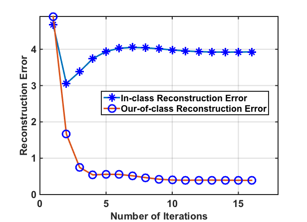
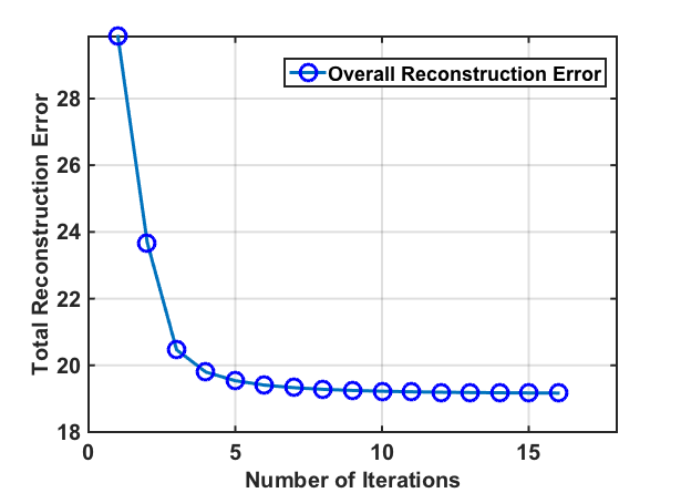
Figure 1: Convergence performance on extended YaleB face recognition dataset. (a) shows the overall reconstruction error; (b) shows the in-class and the out-of-class reconstruction error.

Convergence: This procedure is guaranteed to converge in terms of the objective function value via the following argument. Because each subproblem is convex, the value of the objective function is nondecreasing as iterations proceed. Furthermore, because the objective function is bounded below, the nondecreasing sequence of function values must converge. A sample trajectory is shown in Fig. 1(a). Here, K-SLD2 is trained on the extended YaleB dataset. The overall reconstruction error is shown in (50), whereas Fig. 1(b), shows both that the signal Yisubscript𝑌𝑖Y_{i} is well represented by the dictionary pair (𝐀i,𝐁i)subscript𝐀𝑖subscript𝐁𝑖(\mathbf{A}_{i},\mathbf{B}_{i}) and as the number of iterations increases the other dictionary pairs (𝐀l,𝐁l),lisubscript𝐀𝑙subscript𝐁𝑙𝑙𝑖(\mathbf{A}_{l},\mathbf{B}_{l}),l\neq i start loosing their ability to represent Yisubscript𝑌𝑖Y_{i}.

Classification Procedure: Given a test signal 𝐘𝐘\mathbf{Y} to classify, we first find the coefficient matrices for each class using

{𝐗^i}=argmin{𝐗i}i=1L𝐘l=1L𝐀l𝐗l𝐁lTF2.superscript^𝐗𝑖subscriptsuperscriptsubscriptsuperscript𝐗𝑖𝑖1𝐿superscriptsubscriptnorm𝐘superscriptsubscript𝑙1𝐿subscript𝐀𝑙superscript𝐗𝑙superscriptsubscript𝐁𝑙𝑇𝐹2\{\mathbf{\hat{X}}^{i}\}=\arg\,\min_{\{\mathbf{X}^{i}\}_{i=1}^{L}}||\mathbf{Y}-\sum_{l=1}^{L}\mathbf{A}_{l}\mathbf{X}^{l}\mathbf{B}_{l}^{T}||_{F}^{2}. (55)

This problem is convex and has a closed-form solution. Then, we compute the reconstruction error for each class-specific dictionary:

ei=𝐘𝐀i𝐗^i𝐁iTF2.subscript𝑒𝑖superscriptsubscriptnorm𝐘subscript𝐀𝑖superscript^𝐗𝑖superscriptsubscript𝐁𝑖𝑇𝐹2e_{i}=||\mathbf{Y}-\mathbf{A}_{i}\mathbf{\hat{X}}^{i}\mathbf{B}_{i}^{T}||_{F}^{2}. (56)

Finally, we make the prediction k^=argmini=1,,L(ei)^𝑘subscript𝑖1𝐿subscript𝑒𝑖\hat{k}=\arg\min_{i=1,\cdots,L}(e_{i}); i.e., the class with the smallest reconstruction error.

Computational Complexity: In this analysis we use the fact that: 1) if 𝐀m1×n1𝐀superscriptsubscript𝑚1subscript𝑛1\mathbf{A}\in\mathbb{R}^{m_{1}\times n_{1}} and 𝐗𝐑n1×n2𝐗superscript𝐑subscript𝑛1subscript𝑛2\mathbf{X}\in\mathbf{R}^{n_{1}\times n_{2}} then the matrix multiplication 𝐀𝐗𝐀𝐗\mathbf{A}\mathbf{X} has complexity m1n1n2subscript𝑚1subscript𝑛1subscript𝑛2m_{1}n_{1}n_{2}. 2) if a non singular matrix 𝐀n1×n1𝐀superscriptsubscript𝑛1subscript𝑛1\mathbf{A}\in\mathbb{R}^{n_{1}\times n_{1}}, then 𝐀1superscript𝐀1\mathbf{A}^{-1} has complexity n13superscriptsubscript𝑛13n_{1}^{3}. We obtain a complexity (in terms of matrix multiplications and additions) of

𝒪(KLn1m2(m1+n2)).𝒪𝐾𝐿subscript𝑛1subscript𝑚2subscript𝑚1subscript𝑛2\mathcal{O}(KLn_{1}m_{2}(m_{1}+n_{2})).

If we assume m1=m2=msubscript𝑚1subscript𝑚2𝑚m_{1}=m_{2}=\sqrt{m} and n1=n2=nsubscript𝑛1subscript𝑛2𝑛n_{1}=n_{2}=\sqrt{n} then the complexity becomes

𝒪(KL(mn+nm)).𝒪𝐾𝐿𝑚𝑛𝑛𝑚\mathcal{O}(KL(m\sqrt{n}+n\sqrt{m})).

Which is a reduction when compared to standard subspace learning with computational complexity of 𝒪(KLnm).𝒪𝐾𝐿𝑛𝑚\mathcal{O}(KLnm).

VI Numerical Results

In this section, we evaluate first demonstrate that the empirical classification performance, when the classes are perfectly known, agrees with the diversity order and bounds derived above. Then, we demonstrate the learning and classification performance of K-SLD2 on both synthetic and real-world data.

VI-A Diversity Order

VI-A1 Synthetic Data

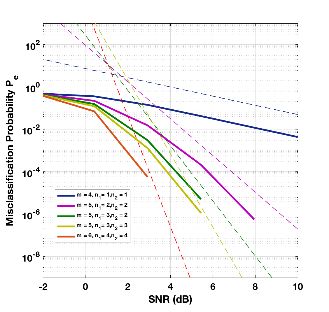
We randomly choose two classes by drawing matrix pairs 𝐀isubscript𝐀𝑖\mathbf{A}_{i} and 𝐁isubscript𝐁𝑖\mathbf{B}_{i} independently from the distribution in (7). Then, we draw data samples i.i.d. from the class-conditional densities in (3). We classify each data sample by minimizing the Mahalanobis distance associated with the covariance of each class-conditional density. We consider five cases, in which we fix m1=m2=msubscript𝑚1subscript𝑚2𝑚m_{1}=m_{2}=m and vary n1subscript𝑛1n_{1} and n2subscript𝑛2n_{2}. In Fig.2 we plot the misclassification probability Pesubscript𝑃𝑒P_{e} against the SNR in dB, averaged over 105superscript10510^{5} random draws from each class. We also plot the upper bound on misclassification probability in terms of principal angles for each case described in (LABEL:Eq:principal). Where dotted colored line shows the misclassification probability associated with the corresponding solid line for each case. In each case, the empirical performance agrees with the diversity predictions with an offset. This offset is large when the ambient signal dimension is small and with large dimensions this offset approaches to zero.
Refer to caption
Figure 2: Misclassification probability Pesubscript𝑃𝑒P_{e} Vs. SNR

VI-B Dictionary Learning Algorithm

In this section we evaluate the performance of K-SLD2 algorithm on synthetic data and two real world datasets: extended YaleB face dataset [40] and the UCI EEG dataset [41], which differentiates the EEG signals of control patients and those who suffer from alcoholism. We compare the performance to state-of-the-art dictionary learning methods such as FDDL [26], DLSI [13], LRSDL [27], standard subspace learning (SSL) using (1) as a baseline method, and the standard kernel support vector machine (SVM). We perform learning and classification on unprocessed signals. When appropriate, we choose model hyper-parameters via cross-validation.

VI-B1 Synthetic data

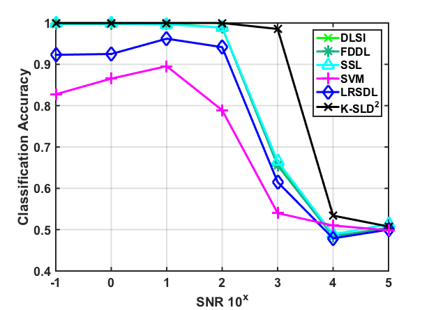
We consider two class classification problem where we draw two matrix pairs 𝐀isubscript𝐀𝑖\mathbf{A}_{i} and 𝐁isubscript𝐁𝑖\mathbf{B}_{i} independently from (7) and draw data samples i.i.d from the class-conditional densities in (3). For this experiment we choose the dimensions of the signal to be 32×32323232\times 32 which lies on the row and column subspaces of dimension 131313 and 171717, respectively. For each class we draw 10 samples for training/dictionary learning and 50 samples for testing. In total we have 60 samples per class. For learning K-S dictionaries using K-SLD2 we use the 2-D signal as it is while for the other learning algorithms we first vectorize the signal (dimension 1024×1102411024\times 1). Fig. 3 compares the performance of learned dictionaries using different methods as the SNR decreases. When the noise power is low, that is, 101absentsuperscript101\leq 10^{1}, standard subspace learning and K-SLD2 performs equally well, but as the noise power increases a significant gain in performance is observed as evident in Fig. 3. We find best classification performance for SVM with polynomial kernel of degree 3.
Refer to caption
Figure 3: Classification accuracy Vs. SNR for synthetic data

VI-B2 Face Recognition

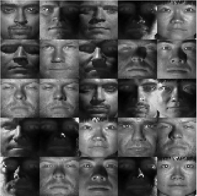
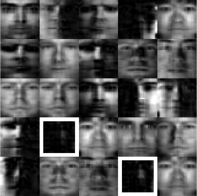
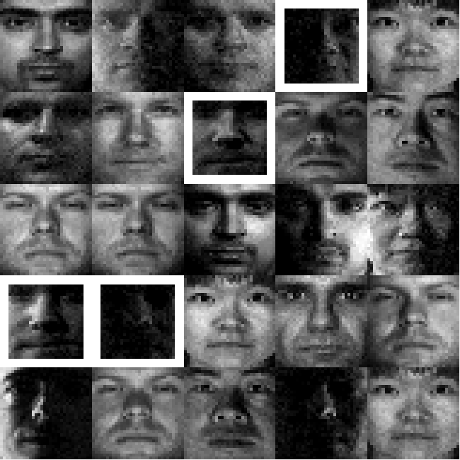
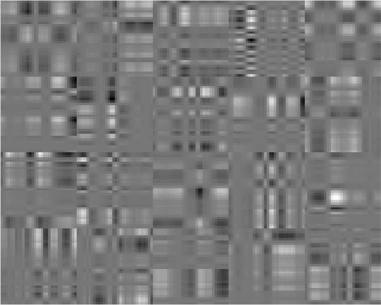
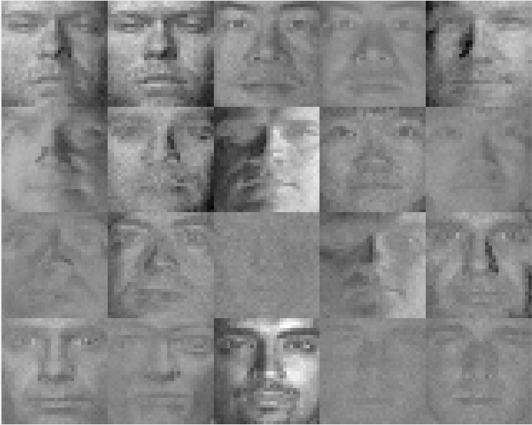
The extended YaleB dataset consists of 2,414 frontal face images from 38 individuals captured under varying lighting conditions. For each class, we use 10 images for training/dictionary learning and the remaining 54 images for testing. In Figure 4 we show the dictionaries learned by K-SLD2 vs. a standard subspace learning model, and we observe that the standard model learns dictionary atoms that look similar to a few reference faces for each class, whereas the K-SLD2 learns more abstract dictionary atoms. This is in part due to imposition of the Kronecker structure on the dictionary atoms, as well as the larger number of atoms possible in a K-S dictionary.
Refer to caption
(a)
Refer to caption
(b)
Figure 4: A subset of dictionary atoms learned by (a) K-SLD2 model, and (b) standard subspace model.
Refer to caption
(a)
Refer to caption
(b)
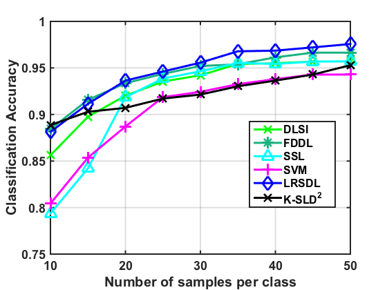
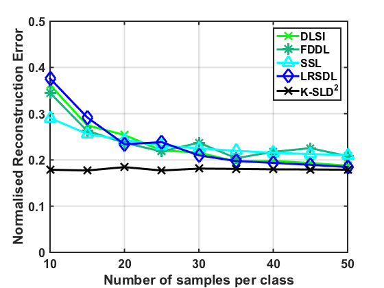
Figure 5: Performance on extended YaleB dataset (a) classification accuracy (b) normalized reconstruction error
SSL
DLSI
FDDL
LRSDL
SVM
K-SLD2
Test sample
classification accuracy (%)
79.36 85.62 88.43 88.14 80.43 88.86
Number of
parameters for representation
102400 102400 102400 similar-to\sim102400 similar-to\sim102400 9600
Average training
time (sec)
0.034 1.2697 9.3254 50.5129 2.234 0.111035
Normalized
reconstruction error
0.290 0.363 0.346 0.376 0.178
TABLE I: Comparison between different approaches for extended YaleB face recognition dataset.

The best hyper-parameters for K-SLD2 turn out to be n1=13subscript𝑛113n_{1}=13, n2=17subscript𝑛217n_{2}=17, and μ=0.9𝜇0.9\mu=0.9. For standard subspace model, we obtain the best classification accuracy for 101010 dictionary atoms. The K-SLD2 uses more atoms overall, but each atom is described by fewer parameters. In Table I, we compare the classification accuracy of K-SLD2 with the other dictionary learning methods. K-SLD2 offers better performance in this case, rather close to FDDL and correctly classify 11.16% of the images than the baseline method. Furthermore, K-SLD2 learns a much more compact model, needing on the order of 1/101101/10th of the parameters of any other method.

We also calculate the normalized reconstruction error (NRE) for all the learning algorithms as follows:

NRE=𝐘𝐘^2𝐘2,NREsuperscriptnorm𝐘^𝐘2superscriptnorm𝐘2\text{NRE}=\frac{||\mathbf{Y}-\mathbf{\hat{Y}}||^{2}}{||\mathbf{Y}||^{2}},

where 𝐘𝐘\mathbf{Y} is the signal of interest and 𝐘^^𝐘\mathbf{\hat{Y}} is the reconstructed signal. Table I shows that K-SLD2 provides the smallest NRE, reducing the error by 38.19% over the baseline. Finally, we observe that the computational complexity, measured in training runtime on a standard desktop computer, is small. LRSDL method requires 50.51 seconds for training while K-SLD2 model requires only 0.11 seconds.
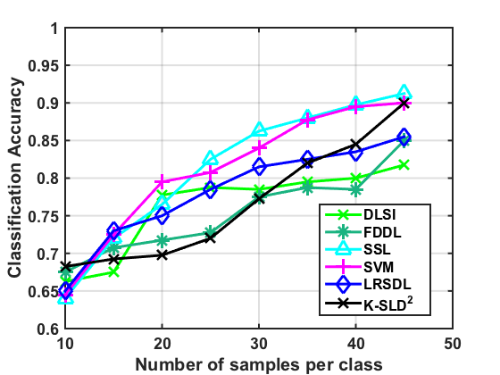
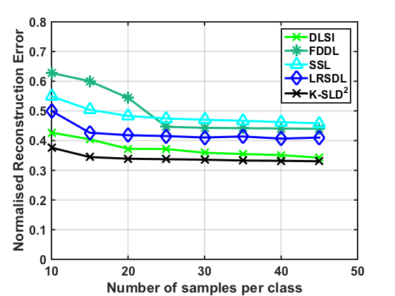
Refer to caption
(a)
Refer to caption
(b)
Figure 6: Performance on EEG Signal dataset (a) classification accuracy (b) normalized reconstruction error
Refer to caption
(a)
Refer to caption
(b)
Refer to caption
(c)
Figure 7: (a) A subset of test samples; (b) Image reconstruction and classification using K-S dictionary (K-SLD2); (c) Image reconstruction and classification using standard subspace dictionary; {White box indicates incorrect classification}

We show the classification and representation performance as a function of the size of the training set in Figs. 5(a) and 5(b), respectively. When the number of samples for training is very small, say 10 samples per class, K-SLD2 model performance is superior, owing in part to the compact model. However, other methods outperform K-SLD2 as the number of samples increases. On the other hand, the reconstruction error of K-SLD2 model is always smaller than other methods for any number of training samples as evident in Fig. 5(b). In Fig. 7, we show a subset of raw YaleB face images used for the reconstruction and classification and compare the performance of K-SLD2 with SSL, where face in white box are the ones with the wrong label prediction.

VI-B3 EEG Dataset

We evaluate the performance of K-SLD2 on the UCI EEG dataset [41], where EEG from the brain were recorded by placing the 64 electrodes on the scalp sampled at 256 Hz for 1 second to examine the correlation of EEG signal to an individual’s alcoholism. Here, we obtain a 2-D signal with electrodes on one axis and the corresponding electrical signal time series on the other. This classification problem is analogous to binary classification having two categories of individuals either belongs to alcoholism or controlled group. The full datasets contains 120 trials for 122 subjects. Similar to YaleB face recognition dataset, we use 10 signals per class for training/dictionary learning and the remaining images for testing and find the value of n1=10subscript𝑛110n_{1}=10 and n2=6subscript𝑛26n_{2}=6 using cross-validation.

SSL
DLSI
FDDL
LRSDL
SVM
K-SLD2
Test sample
classification accuracy (%)
64 66.25 67.5 65 64.9 68.25
Number of
parameters for representation
163840 163840 163840 similar-to\sim 163840 similar-to\sim 163840 2176
Average training
time (sec)
0.012 0.9546 3.4301 128.6921 1.12 0.04
Normalized
reconstruction error
0.290 0.363 0.346 0.50 0.178
TABLE II: Comparison between different approaches on EEG signal dataset

We compare the performance of K-SLD2 in Table II with other dictionary learning methods. Again, K-SLD2 gives better classification performance and requires very few model parameters. In terms of NRE, K-SLD2 reconstruction error is less than 41% of the best among the other methods. We obtain this performance gain for K-SLD2 because the dictionaries with separable structure are very good at signal representation [30]. Similarly, we plot the classification and reconstruction accuracy in Figs. 6(a) and 6(b), respectively. Here, by contrast to YaleB, we observe competitive performance for a larger number of training samples, due perhaps to the explicitly multidimensional nature of EEG signals. Reconstruction performance, measured in NRE, remains superior to other methods.

VII Conclusion

We derive the performance limits on the classification performance of Kronecker-structured models. We derive an exact expression for the slope of misclassification probability as the noise power goes to zero. In high SNR regime, we derive a more accurate and tighter bound on misclassification probability which is determined by the product of principal angles between Kronecker subspaces. We determine the upper and lower bounds on the rate at which the number of classes can grow as the signal dimension goes to infinity. We have also proposed a dictionary learning algorithm K-SLD2, for fast classification and compact representation of multidimensional signals. This algorithm balances the learning of class-specific, Kronecker-structured subspaces against the learning of an general overcomplete dictionary that allows for the representation of general signals. Finally we show that K-SLD2 has improved classification performance over state-of-the-art dictionary learning methods, especially when the size of the training set is small, and competitive reconstruction performance in general.

Appendix A Diversity order gap

Given the K-S diversity order dK-Ssubscript𝑑K-Sd_{\text{K-S}} and the standard subspace diversity order dSTDsubscript𝑑STDd_{\text{STD}}. We derive the diversity gap

γ𝛾\displaystyle\gamma =[2n1n2m1m2]++[2n1m1]+[2n2m2]+,absentsuperscriptdelimited-[]2subscript𝑛1subscript𝑛2subscript𝑚1subscript𝑚2superscriptdelimited-[]2subscript𝑛1subscript𝑚1superscriptdelimited-[]2subscript𝑛2subscript𝑚2\displaystyle=-[2n_{1}n_{2}-m_{1}m_{2}]^{+}+[2n_{1}-m_{1}]^{+}[2n_{2}-m_{2}]^{+},

in terms of signal dimensions for different regions:
Region 1: m1>2n1subscript𝑚12subscript𝑛1m_{1}>2n_{1} and m2>2n2subscript𝑚22subscript𝑛2m_{2}>2n_{2}
Since m1>2n1subscript𝑚12subscript𝑛1m_{1}>2n_{1} and m2>2n2subscript𝑚22subscript𝑛2m_{2}>2n_{2} therefore, [2n1m1]+=[2n2m2]+=0superscriptdelimited-[]2subscript𝑛1subscript𝑚1superscriptdelimited-[]2subscript𝑛2subscript𝑚20{[2n_{1}-m_{1}]^{+}=}~{}[2n_{2}-m_{2}]^{+}=0 and m1m2>4n1n2subscript𝑚1subscript𝑚24subscript𝑛1subscript𝑛2m_{1}m_{2}>4n_{1}n_{2} makes [2n1n2m1m2]+=0superscriptdelimited-[]2subscript𝑛1subscript𝑛2subscript𝑚1subscript𝑚20[2n_{1}n_{2}-m_{1}m_{2}]^{+}=0.
Region 2: n1<m1<2n1subscript𝑛1subscript𝑚12subscript𝑛1n_{1}<m_{1}<2n_{1} and m2>2n2subscript𝑚22subscript𝑛2m_{2}>2n_{2}
Since m2>2n2subscript𝑚22subscript𝑛2m_{2}>2n_{2} therefore, [2n2m2]+=0superscriptdelimited-[]2subscript𝑛2subscript𝑚20[2n_{2}-m_{2}]^{+}=0 also m1>n1subscript𝑚1subscript𝑛1m_{1}>n_{1} and m2>2n2subscript𝑚22subscript𝑛2m_{2}>2n_{2} implies m1m2>2n1n2subscript𝑚1subscript𝑚22subscript𝑛1subscript𝑛2m_{1}m_{2}>2n_{1}n_{2} therefore,  [2n1n2m1m2]+=0superscriptdelimited-[]2subscript𝑛1subscript𝑛2subscript𝑚1subscript𝑚20[2n_{1}n_{2}-~{}m_{1}m_{2}]^{+}=~{}0.
Region 3: n2<m2<2n2subscript𝑛2subscript𝑚22subscript𝑛2n_{2}<m_{2}<2n_{2} and m1>2n1subscript𝑚12subscript𝑛1m_{1}>2n_{1}
Using the similar argument the diversity gap is 0.
Region 4: n1<m1<2n1subscript𝑛1subscript𝑚12subscript𝑛1n_{1}<m_{1}<2n_{1} and n2<m2<2n2subscript𝑛2subscript𝑚22subscript𝑛2n_{2}<m_{2}<2n_{2}
Since n1<m1<2n1subscript𝑛1subscript𝑚12subscript𝑛1n_{1}<m_{1}<2n_{1} and n2<m2<2n2subscript𝑛2subscript𝑚22subscript𝑛2n_{2}<m_{2}<2n_{2} implies that n1n2<m1m2<4n1n2subscript𝑛1subscript𝑛2subscript𝑚1subscript𝑚24subscript𝑛1subscript𝑛2n_{1}n_{2}<m_{1}m_{2}<4n_{1}n_{2}, this gives rise to two different subregions which are m1m2>2n1n2subscript𝑚1subscript𝑚22subscript𝑛1subscript𝑛2m_{1}m_{2}>2n_{1}n_{2} and m1m2<2n1n2subscript𝑚1subscript𝑚22subscript𝑛1subscript𝑛2m_{1}m_{2}<2n_{1}n_{2}.
For m1m2>2n1n2subscript𝑚1subscript𝑚22subscript𝑛1subscript𝑛2m_{1}m_{2}>2n_{1}n_{2}, n1<m1<2n1subscript𝑛1subscript𝑚12subscript𝑛1n_{1}<m_{1}<2n_{1} and n2<m2<2n2subscript𝑛2subscript𝑚22subscript𝑛2n_{2}<m_{2}<2n_{2} which implies [2n1n2m1m2]+=0superscriptdelimited-[]2subscript𝑛1subscript𝑛2subscript𝑚1subscript𝑚20[2n_{1}n_{2}-m_{1}m_{2}]^{+}=0 we derive the diversity order gap as:

γ𝛾\displaystyle\gamma =[2n1n2m1m2]++[2n1m1]+[2n2m2]+absentsuperscriptdelimited-[]2subscript𝑛1subscript𝑛2subscript𝑚1subscript𝑚2superscriptdelimited-[]2subscript𝑛1subscript𝑚1superscriptdelimited-[]2subscript𝑛2subscript𝑚2\displaystyle=-[2n_{1}n_{2}-m_{1}m_{2}]^{+}+[2n_{1}-m_{1}]^{+}[2n_{2}-m_{2}]^{+}
=(2n1m1)(2n2m2).absent2subscript𝑛1subscript𝑚12subscript𝑛2subscript𝑚2\displaystyle=(2n_{1}-m_{1})(2n_{2}-m_{2}).

On the other hand if m1m2<2n1n2subscript𝑚1subscript𝑚22subscript𝑛1subscript𝑛2m_{1}m_{2}<2n_{1}n_{2}, n1<m1<2n1subscript𝑛1subscript𝑚12subscript𝑛1n_{1}<m_{1}<2n_{1} and n2<m2<2n2subscript𝑛2subscript𝑚22subscript𝑛2n_{2}<m_{2}<2n_{2},

γ𝛾\displaystyle\gamma =[2n1n2m1m2]++[2n1m1]+[2n2m2]+absentsuperscriptdelimited-[]2subscript𝑛1subscript𝑛2subscript𝑚1subscript𝑚2superscriptdelimited-[]2subscript𝑛1subscript𝑚1superscriptdelimited-[]2subscript𝑛2subscript𝑚2\displaystyle=-[2n_{1}n_{2}-m_{1}m_{2}]^{+}+[2n_{1}-m_{1}]^{+}[2n_{2}-m_{2}]^{+}
=(2n1n2m1m2)+(2n1m1)(2n2m2)absent2subscript𝑛1subscript𝑛2subscript𝑚1subscript𝑚22subscript𝑛1subscript𝑚12subscript𝑛2subscript𝑚2\displaystyle=-(2n_{1}n_{2}-m_{1}m_{2})+(2n_{1}-m_{1})(2n_{2}-m_{2})
=2(m1n1)(m2n2).absent2subscript𝑚1subscript𝑛1subscript𝑚2subscript𝑛2\displaystyle=2(m_{1}-n_{1})(m_{2}-n_{2}).

Appendix B Intersection of Kronecker Subspaces

Here we characterize the dimension of intersections of subspaces spanned by Kronecker products of matrices. To the best of our knowledge this result is not in the literature, although its statement is intuitive.

Lemma 4.

Suppose dim[(Ai)(Aj)]=xdimensiondelimited-[]subscript𝐴𝑖subscript𝐴𝑗𝑥\dim[\mathcal{R}(A_{i})\bigcap\mathcal{R}(A_{j})]~{}=~{}x and dim[(Bi)(Bj)]=ydimensiondelimited-[]subscript𝐵𝑖subscript𝐵𝑗𝑦\dim[\mathcal{R}(B_{i})\bigcap\mathcal{R}(B_{j})]~{}=~{}y, where ()\mathcal{R}(\cdot) denotes the range space of a matrix. Then,

dim[(𝐁i𝐀i)(𝐁j𝐀j)]=xy.dimensiondelimited-[]tensor-productsubscript𝐁𝑖subscript𝐀𝑖tensor-productsubscript𝐁𝑗subscript𝐀𝑗𝑥𝑦\dim[\mathcal{R}(\mathbf{B}_{i}\otimes\mathbf{A}_{i})\bigcap\mathcal{R}(\mathbf{B}_{j}\otimes\mathbf{A}_{j})]=xy. (57)
Proof:

From [39, p. 447] for pm1×n1𝑝superscriptsubscript𝑚1subscript𝑛1p\in\mathbb{R}^{m_{1}\times n_{1}} and qm2×n2𝑞superscriptsubscript𝑚2subscript𝑛2q\in\mathbb{R}^{m_{2}\times n_{2}}, we have

(pq)=(p𝐈m2×m2)(𝐈m1×m1q).tensor-product𝑝𝑞tensor-product𝑝subscript𝐈subscript𝑚2subscript𝑚2tensor-productsubscript𝐈subscript𝑚1subscript𝑚1𝑞\mathcal{R}(p\otimes q)=\mathcal{R}(p\otimes\mathbf{I}_{m_{2}\times m_{2}})\bigcap\mathcal{R}(\mathbf{I}_{m_{1}\times m_{1}}\otimes q). (58)

Therefore, we can write the dimension as

dim[(𝐁i𝐀i)(𝐁j𝐀j)]=dim[(𝐁i𝐈m1×m1)(𝐈m2×m2𝐀i)(𝐁j𝐈m1×m1)(𝐈m2×m2𝐀j)].dimensiondelimited-[]tensor-productsubscript𝐁𝑖subscript𝐀𝑖tensor-productsubscript𝐁𝑗subscript𝐀𝑗dimensiondelimited-[]tensor-productsubscript𝐁𝑖subscript𝐈subscript𝑚1subscript𝑚1tensor-productsubscript𝐈subscript𝑚2subscript𝑚2subscript𝐀𝑖tensor-productsubscript𝐁𝑗subscript𝐈subscript𝑚1subscript𝑚1tensor-productsubscript𝐈subscript𝑚2subscript𝑚2subscript𝐀𝑗\dim\left[\mathcal{R}(\mathbf{B}_{i}\otimes\mathbf{A}_{i})\bigcap\mathcal{R}(\mathbf{B}_{j}\otimes\mathbf{A}_{j})\right]=\\ \dim\Big{[}\mathcal{R}(\mathbf{B}_{i}\otimes\mathbf{I}_{m_{1}\times m_{1}})\bigcap\mathcal{R}(\mathbf{I}_{m_{2}\times m_{2}}\otimes\mathbf{A}_{i})\bigcap\\ \mathcal{R}(\mathbf{B}_{j}\otimes\mathbf{I}_{m_{1}\times m_{1}})\bigcap\mathcal{R}(\mathbf{I}_{m_{2}\times m_{2}}\otimes\mathbf{A}_{j})\Big{]}. (59)

Rearranging terms, we obtain

dim[(𝐁i𝐀i)(𝐁j𝐀j)]=dim[[(𝐁i𝐈m1×m1)(𝐁j𝐈m1×m1)][(𝐈m2×m2𝐀i)(𝐈m2×m2𝐀j)]].dimensiondelimited-[]tensor-productsubscript𝐁𝑖subscript𝐀𝑖tensor-productsubscript𝐁𝑗subscript𝐀𝑗dimensiondelimited-[]delimited-[]tensor-productsubscript𝐁𝑖subscript𝐈subscript𝑚1subscript𝑚1tensor-productsubscript𝐁𝑗subscript𝐈subscript𝑚1subscript𝑚1delimited-[]tensor-productsubscript𝐈subscript𝑚2subscript𝑚2subscript𝐀𝑖tensor-productsubscript𝐈subscript𝑚2subscript𝑚2subscript𝐀𝑗\dim\left[\mathcal{R}(\mathbf{B}_{i}\otimes\mathbf{A}_{i})\bigcap\mathcal{R}(\mathbf{B}_{j}\otimes\mathbf{A}_{j})\right]=\\ \dim\Big{[}\left[\mathcal{R}(\mathbf{B}_{i}\otimes\mathbf{I}_{m_{1}\times m_{1}})\bigcap\mathcal{R}(\mathbf{B}_{j}\otimes\mathbf{I}_{m_{1}\times m_{1}})\right]\\ \bigcap\left[\mathcal{R}(\mathbf{I}_{m_{2}\times m_{2}}\otimes\mathbf{A}_{i})\bigcap\mathcal{R}(\mathbf{I}_{m_{2}\times m_{2}}\otimes\mathbf{A}_{j})\right]\Big{]}. (60)

Next, let 𝐀ijsubscript𝐀𝑖𝑗\mathbf{A}_{ij} and 𝐁ijsubscript𝐁𝑖𝑗\mathbf{B}_{ij} be matrices whose column spans are (𝐀i)(𝐀j)subscript𝐀𝑖subscript𝐀𝑗\mathcal{R}(\mathbf{A}_{i})\bigcap\mathcal{R}(\mathbf{A}_{j}) and (𝐁i)(𝐁j)subscript𝐁𝑖subscript𝐁𝑗\mathcal{R}(\mathbf{B}_{i})\bigcap\mathcal{R}(\mathbf{B}_{j}), respectively. It is straightforward to verify that

(𝐁i𝐈m1×m1)(𝐁j𝐈m1×m1)=(𝐁ij𝐈m1×m1),tensor-productsubscript𝐁𝑖subscript𝐈subscript𝑚1subscript𝑚1tensor-productsubscript𝐁𝑗subscript𝐈subscript𝑚1subscript𝑚1tensor-productsubscript𝐁𝑖𝑗subscript𝐈subscript𝑚1subscript𝑚1\mathcal{R}(\mathbf{B}_{i}\otimes\mathbf{I}_{m_{1}\times m_{1}})\bigcap\mathcal{R}(\mathbf{B}_{j}\otimes\mathbf{I}_{m_{1}\times m_{1}})=\mathcal{R}(\mathbf{B}_{ij}\otimes\mathbf{I}_{m_{1}\times m_{1}}), (61)

and

(𝐈m2×m2𝐀i)(𝐈m2×m2𝐀j)=(𝐈m2×m2𝐀ij).tensor-productsubscript𝐈subscript𝑚2subscript𝑚2subscript𝐀𝑖tensor-productsubscript𝐈subscript𝑚2subscript𝑚2subscript𝐀𝑗tensor-productsubscript𝐈subscript𝑚2subscript𝑚2subscript𝐀𝑖𝑗\mathcal{R}(\mathbf{I}_{m_{2}\times m_{2}}\otimes\mathbf{A}_{i})\bigcap\mathcal{R}(\mathbf{I}_{m_{2}\times m_{2}}\otimes\mathbf{A}_{j})=\mathcal{R}(\mathbf{I}_{m_{2}\times m_{2}}\otimes\mathbf{A}_{ij}). (62)

Therefore, we can rewrite the subspace dimension as

dim[(𝐁i𝐀i)(𝐁j𝐀j)]=dim[(𝐁ij𝐈m1×m1)(𝐈m2×m2𝐀ij)].dimensiondelimited-[]tensor-productsubscript𝐁𝑖subscript𝐀𝑖tensor-productsubscript𝐁𝑗subscript𝐀𝑗dimensiondelimited-[]tensor-productsubscript𝐁𝑖𝑗subscript𝐈subscript𝑚1subscript𝑚1tensor-productsubscript𝐈subscript𝑚2subscript𝑚2subscript𝐀𝑖𝑗\dim\left[\mathcal{R}(\mathbf{B}_{i}\otimes\mathbf{A}_{i})\bigcap\mathcal{R}(\mathbf{B}_{j}\otimes\mathbf{A}_{j})\right]=\\ \dim\left[\mathcal{R}(\mathbf{B}_{ij}\otimes\mathbf{I}_{m_{1}\times m_{1}})\bigcap\mathcal{R}(\mathbf{I}_{m_{2}\times m_{2}}\otimes\mathbf{A}_{ij})\right]. (63)

Next, we can apply the lemma of [39, p. 447] in reverse, yielding

dim[(𝐁i𝐀i)(𝐁j𝐀j)]dimensiondelimited-[]tensor-productsubscript𝐁𝑖subscript𝐀𝑖tensor-productsubscript𝐁𝑗subscript𝐀𝑗\displaystyle\dim[\mathcal{R}(\mathbf{B}_{i}\otimes\mathbf{A}_{i})\bigcap\mathcal{R}(\mathbf{B}_{j}\otimes\mathbf{A}_{j})] =dim[(𝐁ij𝐀ij)]absentdimensiondelimited-[]tensor-productsubscript𝐁𝑖𝑗subscript𝐀𝑖𝑗\displaystyle=\dim[\mathcal{R}(\mathbf{B}_{ij}\otimes\mathbf{A}_{ij})]
=r(𝐁ij)r(𝐀ij)absent𝑟subscript𝐁𝑖𝑗𝑟subscript𝐀𝑖𝑗\displaystyle=r(\mathbf{B}_{ij})\cdot r(\mathbf{A}_{ij})
=xy.absent𝑥𝑦\displaystyle=xy.

Appendix C Proof of Theorem 2

Expanding the Bhattacharyya bound from (15) we obtain the misclassification probability bound in terms of λijsubscript𝜆𝑖𝑗\lambda_{ij} the nonzero eigenvalues of 𝐃i𝐃iT+𝐃j𝐃jTsubscript𝐃𝑖superscriptsubscript𝐃𝑖𝑇subscript𝐃𝑗superscriptsubscript𝐃𝑗𝑇\mathbf{D}_{i}\mathbf{D}_{i}^{T}+\mathbf{D}_{j}\mathbf{D}_{j}^{T} in (18) as:

Pe(𝐃i,𝐃j)subscript𝑃𝑒subscript𝐃𝑖subscript𝐃𝑗\displaystyle P_{e}(\mathbf{D}_{i},\mathbf{D}_{j}) 12(1σ2)rijn1n22absent12superscript1superscript𝜎2subscriptsuperscript𝑟𝑖𝑗subscript𝑛1subscript𝑛22\displaystyle\leq\frac{1}{2}\left(\frac{1}{\sigma^{2}}\right)^{-\frac{r^{*}_{ij}-n_{1}n_{2}}{2}}
(l=1rij(λijl+σ2)l=1n1n2(λil+σ2)l=1n1n2(λjl+σ2))12absentsuperscriptsuperscriptsubscriptproduct𝑙1subscriptsuperscript𝑟𝑖𝑗subscript𝜆𝑖𝑗𝑙superscript𝜎2superscriptsubscriptproduct𝑙1subscript𝑛1subscript𝑛2subscript𝜆𝑖𝑙superscript𝜎2superscriptsubscriptproduct𝑙1subscript𝑛1subscript𝑛2subscript𝜆𝑗𝑙superscript𝜎212\displaystyle\,\cdot\left(\frac{\prod_{l=1}^{r^{*}_{ij}}(\lambda_{ijl}+\sigma^{2})}{\sqrt{\prod_{l=1}^{n_{1}n_{2}}(\lambda_{il}+\sigma^{2})\cdot\prod_{l=1}^{n_{1}n_{2}}(\lambda_{jl}+\sigma^{2})}}\right)^{-\frac{1}{2}}
=2n1n222(1σ2)rijn1n22absentsuperscript2subscript𝑛1subscript𝑛222superscript1superscript𝜎2subscriptsuperscript𝑟𝑖𝑗subscript𝑛1subscript𝑛22\displaystyle=2^{\frac{n_{1}n_{2}-2}{2}}\cdot\left(\frac{1}{\sigma^{2}}\right)^{-\frac{r^{*}_{ij}-n_{1}n_{2}}{2}}
(l=1rijλijll=1n1n2λill=1n1n2λjl)12+o((σ2)rijn1n22)absentsuperscriptsuperscriptsubscriptproduct𝑙1subscriptsuperscript𝑟𝑖𝑗subscript𝜆𝑖𝑗𝑙superscriptsubscriptproduct𝑙1subscript𝑛1subscript𝑛2subscript𝜆𝑖𝑙superscriptsubscriptproduct𝑙1subscript𝑛1subscript𝑛2subscript𝜆𝑗𝑙12𝑜superscriptsuperscript𝜎2subscriptsuperscript𝑟𝑖𝑗subscript𝑛1subscript𝑛22\displaystyle\,\cdot\left(\frac{\prod_{l=1}^{r^{*}_{ij}}\lambda_{ijl}}{\sqrt{\prod_{l=1}^{n_{1}n_{2}}\lambda_{il}\cdot\prod_{l=1}^{n_{1}n_{2}}\lambda_{jl}}}\right)^{-\frac{1}{2}}+o((\sigma^{2})^{\frac{r^{*}_{ij}-n_{1}n_{2}}{2}}) (64)

Now, our aim is to expand l=1rijλijlsuperscriptsubscriptproduct𝑙1subscriptsuperscript𝑟𝑖𝑗subscript𝜆𝑖𝑗𝑙\prod_{l=1}^{r^{*}_{ij}}\lambda_{ijl} in terms of principal angles.

l=1rijλijl=pdet(Ui,λi,Ui,T+Uj,λj,Uj,T+Ui,λi,Ui,T+Uj,λj,Uj,T).superscriptsubscriptproduct𝑙1subscriptsuperscript𝑟𝑖𝑗subscript𝜆𝑖𝑗𝑙pdetsubscript𝑈𝑖subscript𝜆𝑖superscriptsubscript𝑈𝑖𝑇subscript𝑈𝑗subscript𝜆𝑗superscriptsubscript𝑈𝑗𝑇subscript𝑈𝑖subscript𝜆𝑖superscriptsubscript𝑈𝑖𝑇subscript𝑈𝑗subscript𝜆𝑗superscriptsubscript𝑈𝑗𝑇\prod_{l=1}^{r^{*}_{ij}}\lambda_{ijl}=\mathrm{pdet}(U_{i,\cap}\lambda_{i,\cap}U_{i,\cap}^{T}+U_{j,\cap}\lambda_{j,\cap}U_{j,\cap}^{T}+\\ U_{i,\setminus}\lambda_{i,\setminus}U_{i,\setminus}^{T}+U_{j,\setminus}\lambda_{j,\setminus}U_{j,\setminus}^{T}).

As the image of Ui,subscript𝑈𝑖U_{i,\cap} is orthogonal to Ui,subscript𝑈𝑖U_{i,\setminus} we can write:

l=1rijλijl=pdet(Ui,λi,Ui,T+Uj,λj,Uj,T)×pdet(Ui,λi,Ui,T+Uj,λj,Uj,T).superscriptsubscriptproduct𝑙1subscriptsuperscript𝑟𝑖𝑗subscript𝜆𝑖𝑗𝑙pdetsubscript𝑈𝑖subscript𝜆𝑖superscriptsubscript𝑈𝑖𝑇subscript𝑈𝑗subscript𝜆𝑗superscriptsubscript𝑈𝑗𝑇pdetsubscript𝑈𝑖subscript𝜆𝑖superscriptsubscript𝑈𝑖𝑇subscript𝑈𝑗subscript𝜆𝑗superscriptsubscript𝑈𝑗𝑇\prod_{l=1}^{r^{*}_{ij}}\lambda_{ijl}=\mathrm{pdet}(U_{i,\cap}\lambda_{i,\cap}U_{i,\cap}^{T}+U_{j,\cap}\lambda_{j,\cap}U_{j,\cap}^{T})\times\\ \mathrm{pdet}(U_{i,\setminus}\lambda_{i,\setminus}U_{i,\setminus}^{T}+U_{j,\setminus}\lambda_{j,\setminus}U_{j,\setminus}^{T}).

Following few simple mathematical steps as described in [33] we obtain:

l=1rijλijl=pdet(Ui,λi,Ui,T+Uj,λj,Uj,T)det(λi,)×det(λj,12(𝐈Uj,TUi,Ui,TUj,)λj,12).superscriptsubscriptproduct𝑙1subscriptsuperscript𝑟𝑖𝑗subscript𝜆𝑖𝑗𝑙pdetsubscript𝑈𝑖subscript𝜆𝑖superscriptsubscript𝑈𝑖𝑇subscript𝑈𝑗subscript𝜆𝑗superscriptsubscript𝑈𝑗𝑇detsubscript𝜆𝑖detsuperscriptsubscript𝜆𝑗12𝐈superscriptsubscript𝑈𝑗𝑇subscript𝑈𝑖superscriptsubscript𝑈𝑖𝑇subscript𝑈𝑗superscriptsubscript𝜆𝑗12\prod_{l=1}^{r^{*}_{ij}}\lambda_{ijl}=\mathrm{pdet}(U_{i,\cap}\lambda_{i,\cap}U_{i,\cap}^{T}+U_{j,\cap}\lambda_{j,\cap}U_{j,\cap}^{T})\cdot\mathrm{det}(\lambda_{i,\setminus})\times\\ \mathrm{det}(\lambda_{j,\setminus}^{\frac{1}{2}}(\mathbf{I}-U_{j,\setminus}^{T}U_{i,\setminus}U_{i,\setminus}^{T}U_{j,\setminus})\lambda_{j,\setminus}^{\frac{1}{2}}).

By expanding Ui,,Uj,,Ui,,Uj,subscript𝑈𝑖subscript𝑈𝑗subscript𝑈𝑖subscript𝑈𝑗U_{i,\cap},U_{j,\cap},U_{i,\setminus},U_{j,\setminus} in terms of their row and columns subspace Kronecker products and then following some simple Kronecker product properties we obtain:

l=1rijλijl=pdet(Ui,λi,Ui,T+Uj,λj,Uj,T)det(λi,)×det(λj,12(𝕀(Uj,ATUi,AUi,ATUj,A)(Uj,BTUi,BUi,BTUj,B))λj,12).superscriptsubscriptproduct𝑙1subscriptsuperscript𝑟𝑖𝑗subscript𝜆𝑖𝑗𝑙pdetsubscript𝑈𝑖subscript𝜆𝑖superscriptsubscript𝑈𝑖𝑇subscript𝑈𝑗subscript𝜆𝑗superscriptsubscript𝑈𝑗𝑇detsubscript𝜆𝑖detsuperscriptsubscript𝜆𝑗12𝕀tensor-productsuperscriptsubscript𝑈𝑗𝐴𝑇superscriptsubscript𝑈𝑖𝐴superscriptsubscript𝑈𝑖𝐴𝑇superscriptsubscript𝑈𝑗𝐴superscriptsubscript𝑈𝑗𝐵𝑇superscriptsubscript𝑈𝑖𝐵superscriptsubscript𝑈𝑖𝐵𝑇superscriptsubscript𝑈𝑗𝐵superscriptsubscript𝜆𝑗12\prod_{l=1}^{r^{*}_{ij}}\lambda_{ijl}=\mathrm{pdet}(U_{i,\cap}\lambda_{i,\cap}U_{i,\cap}^{T}+U_{j,\cap}\lambda_{j,\cap}U_{j,\cap}^{T})\cdot\mathrm{det}(\lambda_{i,\setminus})\times\\ \mathrm{det}(\lambda_{j,\setminus}^{\frac{1}{2}}(\mathbb{I}-(U_{j,\setminus}^{AT}U_{i,\setminus}^{A}U_{i,\setminus}^{AT}U_{j,\setminus}^{A})\otimes(U_{j,\setminus}^{BT}U_{i,\setminus}^{B}U_{i,\setminus}^{BT}U_{j,\setminus}^{B}))\lambda_{j,\setminus}^{\frac{1}{2}}).

By careful inspection of det(Uj,ATUi,AUi,ATUj,A)detsuperscriptsubscript𝑈𝑗𝐴𝑇superscriptsubscript𝑈𝑖𝐴superscriptsubscript𝑈𝑖𝐴𝑇superscriptsubscript𝑈𝑗𝐴\mathrm{det}(U_{j,\setminus}^{AT}U_{i,\setminus}^{A}U_{i,\setminus}^{AT}U_{j,\setminus}^{A}) we find that product of eigenvalues of (Uj,ATUi,A)(Uj,ATUi,A)Tsuperscriptsubscript𝑈𝑗𝐴𝑇superscriptsubscript𝑈𝑖𝐴superscriptsuperscriptsubscript𝑈𝑗𝐴𝑇superscriptsubscript𝑈𝑖𝐴𝑇(U_{j,\setminus}^{AT}U_{i,\setminus}^{A})(U_{j,\setminus}^{AT}U_{i,\setminus}^{A})^{T} is the square of the singular values of (Uj,ATUi,A)superscriptsubscript𝑈𝑗𝐴𝑇superscriptsubscript𝑈𝑖𝐴(U_{j,\setminus}^{AT}U_{i,\setminus}^{A}) and are the cosines square of the principal angles between the subspaces. Therefore we obtain:

l=1rijλijl=pdet(Ui,λi,Ui,T+Uj,λj,Uj,T)×l=1n1n2rλi,,ll=1n1n2rλj,,ll=r+1n1n2(1cos2(θl)).superscriptsubscriptproduct𝑙1subscriptsuperscript𝑟𝑖𝑗subscript𝜆𝑖𝑗𝑙pdetsubscript𝑈𝑖subscript𝜆𝑖superscriptsubscript𝑈𝑖𝑇subscript𝑈𝑗subscript𝜆𝑗superscriptsubscript𝑈𝑗𝑇superscriptsubscriptproduct𝑙1subscript𝑛1subscript𝑛2subscript𝑟subscript𝜆𝑖𝑙superscriptsubscriptproduct𝑙1subscript𝑛1subscript𝑛2subscript𝑟subscript𝜆𝑗𝑙superscriptsubscriptproduct𝑙subscript𝑟1subscript𝑛1subscript𝑛21superscript2subscript𝜃𝑙\prod_{l=1}^{r^{*}_{ij}}\lambda_{ijl}=\mathrm{pdet}(U_{i,\cap}\lambda_{i,\cap}U_{i,\cap}^{T}+U_{j,\cap}\lambda_{j,\cap}U_{j,\cap}^{T})\times\\ \prod_{l=1}^{n_{1}n_{2}-r_{\cap}}\lambda_{i,\setminus,l}\cdot\prod_{l=1}^{n_{1}n_{2}-r_{\cap}}\lambda_{j,\setminus,l}\cdot\prod_{l=r_{\cap}+1}^{n_{1}n_{2}}(1-\cos^{2}(\theta_{l})).

In terms of principal angles of individual row and column subspaces we obtain:

l=1rijλijl=pdet(Ui,λi,Ui,T+Uj,λj,Uj,T)×l=1n1n2rλi,,ll=1n1n2rλj,,ll=t1+1n1l=t2+1n2(1cos2(θlA)cos2(θlB)).superscriptsubscriptproduct𝑙1subscriptsuperscript𝑟𝑖𝑗subscript𝜆𝑖𝑗𝑙pdetsubscript𝑈𝑖subscript𝜆𝑖superscriptsubscript𝑈𝑖𝑇subscript𝑈𝑗subscript𝜆𝑗superscriptsubscript𝑈𝑗𝑇superscriptsubscriptproduct𝑙1subscript𝑛1subscript𝑛2subscript𝑟subscript𝜆𝑖𝑙superscriptsubscriptproduct𝑙1subscript𝑛1subscript𝑛2subscript𝑟subscript𝜆𝑗𝑙superscriptsubscriptproduct𝑙subscript𝑡11subscript𝑛1superscriptsubscriptproduct𝑙subscript𝑡21subscript𝑛21superscript2superscriptsubscript𝜃𝑙𝐴superscript2superscriptsubscript𝜃𝑙𝐵\prod_{l=1}^{r^{*}_{ij}}\lambda_{ijl}=\mathrm{pdet}(U_{i,\cap}\lambda_{i,\cap}U_{i,\cap}^{T}+U_{j,\cap}\lambda_{j,\cap}U_{j,\cap}^{T})\times\\ \prod_{l=1}^{n_{1}n_{2}-r_{\cap}}\lambda_{i,\setminus,l}\prod_{l=1}^{n_{1}n_{2}-r_{\cap}}\lambda_{j,\setminus,l}\prod_{l=t_{1}+1}^{n_{1}}\prod_{l=t_{2}+1}^{n_{2}}(1-\cos^{2}(\theta_{l}^{A})\cos^{2}(\theta_{l}^{B})).

Substituting this in (64), we obtain the desired results as stated in Theorem 2.

References

  • [1] K.-C. Lee, J. Ho, and D. J. Kriegman, “Acquiring linear subspaces for face recognition under variable lighting,” IEEE Transactions on pattern analysis and machine intelligence, vol. 27, no. 5, pp. 684–698, 2005.
  • [2] L. Bottou, C. Cortes, J. S. Denker, H. Drucker, I. Guyon, L. D. Jackel, Y. LeCun, U. A. Muller, E. Sackinger, P. Simard et al., “Comparison of classifier methods: a case study in handwritten digit recognition,” in International conference on pattern recognition.   IEEE Computer Society Press, 1994, pp. 77–77.
  • [3] D. A. Reynolds and R. C. Rose, “Robust text-independent speaker identification using gaussian mixture speaker models,” IEEE transactions on speech and audio processing, vol. 3, no. 1, pp. 72–83, 1995.
  • [4] T. Kinnunen and H. Li, “An overview of text-independent speaker recognition: From features to supervectors,” Speech communication, vol. 52, no. 1, pp. 12–40, 2010.
  • [5] D. T. Ross, U. Scherf, M. B. Eisen, C. M. Perou, C. Rees, P. Spellman, V. Iyer, S. S. Jeffrey, M. Van de Rijn, M. Waltham et al., “Systematic variation in gene expression patterns in human cancer cell lines,” Nature genetics, vol. 24, no. 3, pp. 227–235, 2000.
  • [6] S. Soltani, M. E. Kilmer, and P. C. Hansen, “A tensor-based dictionary learning approach to tomographic image reconstruction,” BIT Numerical Mathematics, pp. 1–30, 2015.
  • [7] K. G. Derpanis, M. Lecce, K. Daniilidis, and R. P. Wildes, “Dynamic scene understanding: The role of orientation features in space and time in scene classification,” in Computer Vision and Pattern Recognition (CVPR), 2012 IEEE Conference on.   IEEE, 2012, pp. 1306–1313.
  • [8] S. Tan, Y. Zhang, G. Wang, X. Mou, G. Cao, Z. Wu, and H. Yu, “Tensor-based dictionary learning for dynamic tomographic reconstruction,” Physics in medicine and biology, vol. 60, no. 7, p. 2803, 2015.
  • [9] K. Greenewald, T. Tsiligkaridis, and A. O. Hero, “Kronecker sum decompositions of space-time data,” in Computational Advances in Multi-Sensor Adaptive Processing (CAMSAP), 2013 IEEE 5th International Workshop on.   IEEE, 2013, pp. 65–68.
  • [10] T. Tsiligkaridis and A. O. Hero, “Covariance estimation in high dimensions via Kronecker product expansions,” IEEE Transactions on Signal Processing, vol. 61, no. 21, pp. 5347–5360, 2013.
  • [11] Z. Shakeri, W. U. Bajwa, and A. D. Sarwate, “Minimax lower bounds for Kronecker-structured dictionary learning,” arXiv preprint arXiv:1605.05284, 2016.
  • [12] Q. Zhang and B. Li, “Discriminative K-SVD for dictionary learning in face recognition,” in Computer Vision and Pattern Recognition (CVPR), 2010 IEEE Conference on.   IEEE, 2010, pp. 2691–2698.
  • [13] I. Ramirez, P. Sprechmann, and G. Sapiro, “Classification and clustering via dictionary learning with structured incoherence and shared features,” in Computer Vision and Pattern Recognition (CVPR), 2010 IEEE Conference on.   IEEE, 2010, pp. 3501–3508.
  • [14] Z. Jiang, Z. Lin, and L. S. Davis, “Learning a discriminative dictionary for sparse coding via label consistent K-SVD,” in Computer Vision and Pattern Recognition (CVPR), 2011 IEEE Conference on.   IEEE, 2011, pp. 1697–1704.
  • [15] K. Werner, M. Jansson, and P. Stoica, “On estimation of covariance matrices with Kronecker product structure,” IEEE Transactions on Signal Processing, vol. 56, no. 2, pp. 478–491, 2008.
  • [16] T. Tsiligkaridis, A. O. Hero III, and S. Zhou, “On convergence of kronecker graphical lasso algorithms,” IEEE transactions on signal processing, vol. 61, no. 7, pp. 1743–1755, 2013.
  • [17] P. Dutilleul, “The mle algorithm for the matrix normal distribution,” Journal of statistical computation and simulation, vol. 64, no. 2, pp. 105–123, 1999.
  • [18] F. Renna, L. Wang, X. Yuan, J. Yang, G. Reeves, R. Calderbank, L. Carin, and M. R. Rodrigues, “Classification and reconstruction of high-dimensional signals from low-dimensional features in the presence of side information,” IEEE Transactions on Information Theory, vol. 62, no. 11, pp. 6459–6492, 2016.
  • [19] J. Yang, Z. Wang, Z. Lin, S. Cohen, and T. Huang, “Coupled dictionary training for image super-resolution,” IEEE Transactions on Image Processing, vol. 21, no. 8, pp. 3467–3478, 2012.
  • [20] O. Bryt and M. Elad, “Compression of facial images using the K-SVD algorithm,” Journal of Visual Communication and Image Representation, vol. 19, no. 4, pp. 270–282, 2008.
  • [21] M. Elad and M. Aharon, “Image denoising via sparse and redundant representations over learned dictionaries,” IEEE Transactions on Image processing, vol. 15, no. 12, pp. 3736–3745, 2006.
  • [22] M. Aharon, M. Elad, and A. Bruckstein, “K-SVD: An algorithm for designing overcomplete dictionaries for sparse representation,” IEEE Transactions on signal processing, vol. 54, no. 11, pp. 4311–4322, 2006.
  • [23] K. Engan, S. O. Aase, and J. H. Husoy, “Method of optimal directions for frame design,” in Acoustics, Speech, and Signal Processing, 1999. Proceedings., 1999 IEEE International Conference on, vol. 5.   IEEE, 1999, pp. 2443–2446.
  • [24] Z. Jiang, Z. Lin, and L. S. Davis, “Label consistent K-SVD: Learning a discriminative dictionary for recognition,” IEEE Transactions on Pattern Analysis and Machine Intelligence, vol. 35, no. 11, pp. 2651–2664, 2013.
  • [25] M. Yang, L. Zhang, J. Yang, and D. Zhang, “Metaface learning for sparse representation based face recognition,” in Image Processing (ICIP), 2010 17th IEEE International Conference on.   IEEE, 2010, pp. 1601–1604.
  • [26] M. Yang, L. Zhang, X. Feng, and D. Zhang, “Fisher discrimination dictionary learning for sparse representation,” in Computer Vision (ICCV), 2011 IEEE International Conference on.   IEEE, 2011, pp. 543–550.
  • [27] T. H. Vu and V. Monga, “Fast low-rank shared dictionary learning for image classification,” IEEE Transactions on Image Processing, vol. 26, no. 11, pp. 5160–5175, 2017.
  • [28] G. Duan, H. Wang, Z. Liu, J. Deng, and Y.-W. Chen, “K-CPD: Learning of overcomplete dictionaries for tensor sparse coding,” in Pattern Recognition (ICPR), 2012 21st International Conference on.   IEEE, 2012, pp. 493–496.
  • [29] S. Zubair and W. Wang, “Tensor dictionary learning with sparse tucker decomposition,” in Digital Signal Processing (DSP), 2013 18th International Conference on.   IEEE, 2013, pp. 1–6.
  • [30] S. Hawe, M. Seibert, and M. Kleinsteuber, “Separable dictionary learning,” in Proceedings of the IEEE Conference on Computer Vision and Pattern Recognition, 2013, pp. 438–445.
  • [31] Y. Peng, D. Meng, Z. Xu, C. Gao, Y. Yang, and B. Zhang, “Decomposable nonlocal tensor dictionary learning for multispectral image denoising,” in Proceedings of the IEEE Conference on Computer Vision and Pattern Recognition, 2014, pp. 2949–2956.
  • [32] M. Nokleby, M. Rodrigues, and R. Calderbank, “Discrimination on the grassmann manifold: Fundamental limits of subspace classifiers,” IEEE Transactions on Information Theory, vol. 61, no. 4, pp. 2133–2147, 2015.
  • [33] J. Huang, Q. Qiu, and R. Calderbank, “The role of principal angles in subspace classification,” IEEE Transactions on Signal Processing, vol. 64, no. 8, pp. 1933–1945, 2016.
  • [34] J. Hamm and D. D. Lee, “Grassmann discriminant analysis: a unifying view on subspace-based learning,” in Proceedings of the 25th international conference on Machine learning.   ACM, 2008, pp. 376–383.
  • [35] L. Zheng and D. N. C. Tse, “Diversity and multiplexing: A fundamental tradeoff in multiple-antenna channels,” IEEE Transactions on information theory, vol. 49, no. 5, pp. 1073–1096, 2003.
  • [36] T. Kailath, “The divergence and Bhattacharyya distance measures in signal selection,” IEEE transactions on communication technology, vol. 15, no. 1, pp. 52–60, 1967.
  • [37] A. V. Knyazev and P. Zhu, “Principal angles between subspaces and their tangents,” Technical report TR2012-058, Mitsubishi Electric Research Laboratories, 2012.
  • [38] R. E. Cline and R. Funderlic, “The rank of a difference of matrices and associated generalized inverses,” Linear Algebra and its Applications, vol. 24, pp. 185–215, 1979.
  • [39] D. S. Bernstein, Matrix mathematics: theory, facts, and formulas.   Princeton University Press, 2009.
  • [40] A. S. Georghiades, P. N. Belhumeur, and D. J. Kriegman, “From few to many: Illumination cone models for face recognition under variable lighting and pose,” IEEE transactions on pattern analysis and machine intelligence, vol. 23, no. 6, pp. 643–660, 2001.
  • [41] X. L. Zhang, H. Begleiter, B. Porjesz, W. Wang, and A. Litke, “Event related potentials during object recognition tasks,” Brain Research Bulletin, vol. 38, no. 6, pp. 531–538, 1995.