Multiscaling in Strong Turbulence Driven by a Random Force.

Abstract

Turbulence problem is often considered as “the last unsolved problem of classical physics”. It is due to strong interaction between velocity and/or velocity gradient fluctuations, a high Reynolds number flow is a fascinating mixture of purely random, close to Gaussian, fields and coherent structures where substantial fraction of kinetic energy is dissipated into heat. To evaluate intensity of fluctuations, one usually studies different moments of velocity increments and/or dissipation rate, characterized by scaling exponents $\zeta_{n}$ and $d_{n}$, respectively. In high Reynolds number flows, the moments of different orders with $n\neq m$ cannot be simply related to each other, which is the signature of anomalous scaling, making this problem “the last unsolvable”. No perturbative treatment can lead to quantitative description of this feature. In this work the expressions for the moments of dissipation rate $e_{n}=\overline{{\cal E}^{n}}\propto Re^{d_{n}}$ and those of velocity derivatives $M_{2n}=\overline{(\partial_{x}u_{x})^{2n}}\propto\frac{v_{o}^{2n}}{L^{2n}}Re^{\rho_{2n}}$ are derived for an infinite fluid stirred by a white-in-time Gaussian random force supported in the vicinity of the wave number $k_{f}\approx\frac{2\pi}{L}=O(1)$, where $v_{0}$ and $L$ are characteristic velocity and integral scale, respectively. A novel aspect of this work is that unlike previous efforts which aimed at seeking solutions around the infinite Reynolds number limit, we concentrate on the vicinity of transitional Reynolds numbers $Re^{tr}$ of the first emergence of anomalous scaling out of Low-Re Gaussian background. The obtained closed expressions for anomalous scaling exponents $d_{n}$ and $\rho_{n}$ agree well with available in literature experimental and numerical data and, when $n\gg 1$, $d_{n}\approx 0.3n\ln(n)$.

PACS numbers 47.27

Introduction.

2. “Reynolds numbers” . Definitions. If a velocity gradient field obeys Gaussian statistics with the Re-dependent variance, $\overline{(\partial_{x}v_{x})^{2}}\propto\frac{v_{0}^{2}}{L^{2}}Re^{\rho_{2}}$, its moments $\overline{(\partial_{x}v_{x})^{2n}}=(2n-1)!!(\overline{(\partial_{x}v_{x})^{2}})^{n}\propto\frac{v_{o}^{2n}}{L^{2n}}Re^{n\rho_{2}}$. Here, $v_{0}=O(1.)$ and $L=2\pi/k_{0}=O(1)$ are the single-point large-scale properties of the flow. The above-mentioned“ normal scaling” is not the only possibility. Indeed, high-Reynolds-number flows are characterized by “anomalous” scaling exponents reflecting the formation of coherent structures. In this case $\overline{(\partial_{x}v_{x})^{2n}}\propto\frac{v_{0}^{2n}}{L^{2n}}Re^{\rho_{2n}}$ where $\rho_{2n}\neq n\rho_{2}$. In principle, depending on the dynamics, the transitional Reynolds numbers of different moments $n$ of velocity field may be different and with increase of the Reynolds number above critical one ($Re_{n}^{tr}$), the flow may become a superposition of Gaussian and “anomalous” patches obeying different laws. This fact makes the problem of anomalous scaling or intermittency so difficult.

In general, we have to define an infinite number of large-scale mean velocities $\hat{v}(n)=L\overline{(\partial_{x}v_{x})^{n}}^{\frac{1}{n}}$ and corresponding Reynolds numbers:

$$\hat{R}e_{n}=\hat{v}(n)L/\nu\equiv\frac{L^{2}\overline{(\partial_{x}v_{x})^{n}}^{\frac{1}{n}}}{\nu}\propto Re^{\frac{\rho_{n}}{n}+1}$$ (1)

where $\rho_{n}$ is a scaling exponent of the $n^{th}$ -order moment of velocity derivative, i.e. $\overline{(\partial_{x}v_{x})^{n}}\propto Re^{\rho_{n}}$. As follows from (1),

$$Re\approx\hat{R}e_{n}^{\frac{n}{\rho_{n}+n}}$$ (2)

and, the widely used in hydrodynamics large-scale dimensionless parameter, the “Reynolds number”, is : $Re\equiv\hat{R}e_{2}=\frac{(\partial_{x}v_{x})_{rms}L^{2}}{\nu}$. One can introduce an infinite number of Reynolds numbers based on “Taylor length scales”:

$$\hat{R}_{\lambda,n}=\sqrt{\frac{15L^{4}}{\overline{3{\cal E}\nu}}}\hat{v}(2n)=$$

$$\sqrt{\frac{15v_{0}^{3}}{\overline{3L}{\cal E}}}\sqrt{Re}\times\frac{L^{2}}{v_{0}^{2}}\overline{(\partial_{x}v_{x})^{2n}}^{\frac{1}{n}}\approx Re^{\frac{\rho_{2n}}{n}+\frac{1}{2}}$$ (3)

where dimensionless combination $\frac{{\cal E}L}{v_{0}^{3}}=O(1)$. It clear that the proportionality coefficient in (3) is $n$-independent. This fact will be essential for what follows. Multiplying and dividing right side of (3) by viscosity $\nu$ and taking into account that in the system under consideration ${\cal E}=P=const=O(1)$ (see below), one obtains $Re^{\frac{\rho_{2n}}{n}}\approx Re^{\frac{d_{n}}{n}+1}$ giving

$$\rho_{2n}=d_{n}+n$$

If the flow is generated by a Gaussian random force (see below), in the limit $Re\rightarrow 0$, the velocity field is random and at least the first few low-order moments obey close-to-Gaussian statistics. The question arises: given the random low-Reynolds number flow, how do we define chaotic “strong” turbulence dominating the large-Re dynamics? This problem was addressed in Ref.[1] where we discussed emergence of intermittency out of “normal” Gaussian background with increase of $Re$. A similar question has been studied by Kuz’min and Patashinsky [2] in terms of small-scale phase organization in a low Reynolds number flow.

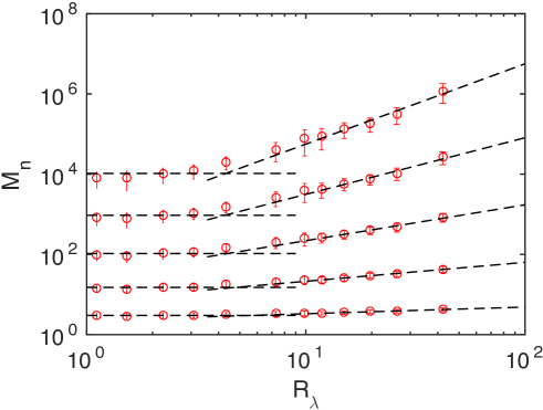
It has been demonstrated both theoretically and numerically in Ref.[1] that transitional Reynolds number $\hat{R}e_{2}^{tr}\equiv Re^{tr}$ from “normal” to “anomalous” scaling of normalized velocity derivatives $M_{2n}=\overline{(\partial_{x}v_{x})^{2n}}\propto(\frac{v_{o}}{L})^{2n}Re^{\rho_{2n}}$ and those of dissipation rates $e_{n}=\overline{{\cal E}^{n}}\propto Re^{d_{n}}$ are $n$-dependent, monotonically decreasing with increase of the moment order $n$ [1],[3] ( also see Fig.1). It was further shown that $Re^{tr}\approx 100$ ($R^{tr}_{\lambda}\approx 9.$) for $2n\approx 4$. However, expressed in terms of $\hat{R}_{\lambda,n}$, the observed transition points $\hat{R}^{tr}_{\lambda,n}$ were $n$-independent with $\hat{R}^{tr}_{\lambda,n}\approx 9.0$. In this paper, using this effect as a dynamic constraint, we generalize the theory developed in [1] to calculate anomalous scaling exponents $\rho_{n}$ and $d_{n}$.

1. Background. In 1965, in his classic textbook [4], R.P. Feynman proclaimed “turbulence as the most important unsolved problem of classical physics”. His point was that by 1965 we knew more about weak and strong interactions of elementary particles than about flow of water out of faucets in our bathtubs. Feynman did not elaborate on his statement and we can only guess that he had in mind a derivation of chaotic, high-Reynolds number solutions directly from deterministic and well-known Navier-Stokes equations for incompressible fluids. By that time it became clear (for a comprehensive review see Refs. [5]) that, due to the lack of a small coupling constant, the problem of derivation of the energy spectra and other correlation functions using renormalized perturbation expansions was at least as hard as that in the theory of strong interactions. At approximately the same time in an extraordinary 1969 paper, Polyakov, developing his theory of strong interactions of hadrons [6], accounted for the multi-particle (high-order) contributions to the diagrammatic expansions of Green functions, leading to the first calculation of anomalous scaling exponents (multiscaling). Unlike scaling solutions in the theory of critical point or Kolmogorov’s similarity relations for the low-order moments of velocity increments, in multiscaling the moments of different orders are characterized by scaling functions of different dimensionalities. To illustrate the physics behind this novel concept, Polyakov constructed a qualitative “cascade model” yielding the calculated scaling exponents. Since 1941 various cascade models leading to Kolmogorov’s energy spectrum, have been well-known (for a very detailed review and discussions see Ref. [5]-[6]). Starting from 1962 Kolmogorov’s attempts to derive anomalous scaling exponents, numerous “cascade models” have been developed to obtain exponents for high-order structure functions and moments of dissipation Regretfully, these ideas, applied to strong turbulence, failed. Anyhow, Feynman’s assessment of the “turbulence problem” has been repeated countless times as an inspiration for various attacks on this problem.
Twenty seven years later, in a Science paper, M.Nelkin, reviewing the status of turbulence research, asked a crucial question: “In What Sense Turbulence in Unsolved Problem?” [7]. Usually, fluid turbulence is a result of instability of a low-Reynolds number laminar flow which is a solution to the Navier-Stokes equations in the limit $Re=VL/\nu\rightarrow 0$, where $V$ and $L$ are free-stream velocity and characteristic flow length-scale, respectively. Since the number of possible laminar flows is, for all practical purpose infinite, one can hardly expect a large-scale universality of both mechanisms of turbulence production and of magnitudes of critical (transitional) Reynolds number. Still, according to Kolmogorov’s theory of 1941, one can expect some universality on the scale $r/L\ll 1$ and it is possible that in this interval the size of the system disappears from the dynamics: the energy spectrum then is given by the scaling law:

$$E(k)=\overline{{\cal E}}^{\frac{2}{3}}k^{-\frac{5}{3}}f(k\eta)$$

where $\eta$ is the dissipation scale (see below). The scaling function $f(x)$ is assumed universal. This relation can be rewritten in physical space

$$S_{2}(r)=\overline{(u(x+r)-u(x))^{2}}=(\overline{{\cal E}}r)^{\frac{2}{3}}f(\frac{r}{\eta})$$ (4)

At the length-scale $r\approx\eta$ viscous effects become important and in the interval $r\ll\eta$, velocity field is an analytic function. It was further assumed that in the inertial range $L\gg r\gg\eta$ the viscous effects are negligibly weak and the scaling function $f(x)\rightarrow C=const$. If this is so, one obtains the so called Kolmogorov’s spectrum $E(k)\propto C{\cal E}^{\frac{2}{3}}k^{-\frac{5}{3}}$ and $S_{2}\propto r^{\frac{2}{3}}$. These considerations, leading to the above “$5/3$ energy spectrum”, are often called in the literature: “Kolmogorov’s K41 theory”. Nelkin stressed that, while there was no solid theoretical derivation of these results, they were quite close to the available at the time experimental data.

The relation (3) leads to an important conclusion: consider $r/\eta\rightarrow 0$. In this limit the velocity field is an analytic function, so that $S_{2}\approx\overline{(\frac{\partial_{x}u_{x}}{\partial x})^{2}}r^{2}=\overline{{\cal E}}r^{2}/(15\nu)$, and we can safely set $r\rightarrow\eta$. Taking into account that, by the energy conservation, $\overline{{\cal E}}L/V^{3}=O(1)$, we, matching analytic and inertial (singular) ranges, obtain $(\frac{\eta}{L})^{\frac{2}{3}}\approx Re(\frac{\eta}{L})^{2}$, which is nothing but Kolmogorov’s relation $\eta=LRe^{-\frac{3}{4}}$ where the large-scale Reynolds number $Re=VL/\nu$. Small correction to Kolmogorov’s spectrum ( $E(k)\propto k^{-0.71}$ ) has been reported (see Ref. [8],[9]).

The situation is totally unsatisfactory when K41 is used to predict high-order moments of velocity increments and dissipation rate. Indeed, K41 gives

$$\overline{{\cal E}^{n}}=\nu^{n}\eta^{\frac{4n}{3}}\approx Re^{0}=const$$

This result contradicted all known experimental data which gave strong indications of Kolmogorov’s theory breakdown at small scales $r\rightarrow\eta$ [5],[7]- [9]. Moreover, the scaling solution

$$S_{n}=r^{-\gamma}\int(\delta_{r}u)^{n}{\cal P}(\frac{\delta_{r}u}{r^{\gamma}})d(\delta_{\eta}u)\propto r^{n\gamma}$$

where $r^{-\gamma}P(x)$ is a scaling function for the normalized probability density (PDF), of velocity increments, failed to describe the experimentally observed multiscaling, defined by the relation $S_{n}\propto r^{\zeta_{n}}$ with the exponents $\zeta_{n}/n\neq\zeta_{m}/m$ for $n\neq m$. Nelkin stressed the inability of scaling theory to describe the moments of dissipation rate $e_{n}=\overline{{\cal E}^{n}}\propto Re^{d_{n}}$ as the main deficiency of exiting turbulence theory. This was one of his reasons to deem turbulence problem “the last…”.

The failure of the formula $\eta\propto LRe^{-\frac{3}{4}}$ has been relatively recently theoretically predicted and detected in very accurate numerical simulations [9], where it was shown that the more accurate dependence was $\eta\equiv\eta_{2}=LRe^{-0.78}$. While this deviation from Kolmogorov’s $\eta_{2}\approx LRe^{-0.75}$ can be regarded as small, the experimentally observed “dissipation scales” $\eta_{n}\approx LRe^{-\theta_{n}}$, with with $n>2$, very strongly deviated from Kolmogorov’s value $\theta_{n}=3/4$. The length-scales $\eta_{n}$ are defined as follows: $S_{n}=\overline{(u(x+r)-u(x))^{n}}\propto r^{n}$ when $r/\eta_{n}\ll 1$. The explanation of this phenomenon is hidden deep in the dynamics of turbulence and turbulence transition. If, following Landau/Lifshitz, one assumes [10] that turbulence transition happens locally when $Re_{r}=(\delta_{r}u)r/\nu\geq 1$, one concludes that the flow is a superposition of turbulent ($Re_{r}>1$) and laminar ($Re_{r}<1$), patches. Therefore, locally, the dissipation (viscous) scale, given by $Re_{\eta}\approx 1$ or

$$\eta\approx\nu/\delta_{\eta}u$$ (5)

is a strongly fluctuating parameter depending on the local magnitude of $\delta_{\eta}u$. That is where Kolmogorov’s theory breaks down giving rise to huge anomalous fluctuations of all spatial derivatives, including dissipation rate ${\cal E}$. The relation (5) gives the low bound on the “dissipation scale”. It is clear that the largest velocity fluctuations are $u\approx u_{rms}$. Indeed due to the Gaussian statistics of large-scale fluctuations, the probability of an event $u>u_{rms}$ is very small. Substituting this estimate into (4) gives in the high-Re limit:

$$\eta_{min}/L\approx 1/Re<<Re^{-\frac{3}{4}}$$

In the limit $Re\rightarrow\infty$, huge fluctuations of dissipation scale make renormalized perturbations expansions problematic.

In this paper we develop a quantitative theory for the moments of velocity derivative in a particular problem of a random-force-driven Navier-Stokes turbulence.

The model. Fluid flow can be described by the Navier-Stokes equations subject to boundary and initial conditions (the density is taken $\rho=1$ without loss of generality):

$$\partial_{t}{\bf u}+{\bf u\cdot\nabla u}=-\nabla p+\nu\nabla^{2}{\bf u}+{\bf f}$$ (6)

$\nabla\cdot{\bf u}=0$. A random Gaussian noise ${\bf f}$ is defined by the correlation function [10],[11]:

$$\overline{f_{i}({\bf k},\omega)f_{j}({\bf k^{\prime}},\omega^{\prime})}=(2\pi)^{d+1}D_{0}(k)P_{ij}({\bf k})\delta({\hat{k}+\hat{k}^{\prime}})$$ (7)

where the four-vector $\hat{k}=({\bf k},\omega)$ and projection operator is: $P_{ij}({\bf k})=\delta_{ij}-\frac{k_{i}k_{j}}{k^{2}}$. In equilibrium fluid the thermal fluctuations, responsible for Brownian motion are generated by the forcing (6) with $D_{0}(k)=\frac{k_{B}T\nu}{\rho}k^{2}$ [10],[11]. In channel flows or boundary layers with rough walls, the amplitude $D_{0}$ is of the order of the rms magnitude of the roughness element [2]. Here we are interested in the case $D_{0}(k)=const\neq 0$ only in the interval close to $k\approx 2\pi/L$, discussed by Forster, Nelson and Stephen [11]. The energy balance, written here for the case of isotropic and homogeneous flow, following from (5) -(6) imposes the energy conservation constraint: ${\cal P}=\overline{{\bf u}\cdot{\bf f}}={\cal E}=\frac{\nu}{2}\overline{(\frac{\partial u_{i}}{\partial x_{j}}+\frac{\partial u_{j}}{\partial x_{i}})^{2}}=\nu\overline{(\frac{\partial u_{i}}{\partial x_{j}})^{2}}=O(1)$, where energy production rate ${\cal P}=O(1)$ is an external parameter independent upon Reynolds number. The random-force-driven NS equation can be written in the Fourier space:

$$u_{l}({\bf k},\omega)=G^{0}f_{l}({\bf k,\omega})-\frac{i}{2}G^{0}{\cal P}_{lmn}\int u_{m}({\bf q},\Omega)u_{n}({\bf k-q},\omega-\Omega)d{\bf Q}d\Omega$$ (8)

where $G^{0}=(-i\omega+\nu k^{2})^{-1}$, ${\cal P}_{lmn}({\bf k})=k_{n}P_{lm}({\bf k})+k_{m}P_{ln}({\bf k})$ and, introducing the zero-order solution ${\bf u}_{0}=G^{0}{\bf f}\propto\sqrt{D_{0}}$, so that ${\bf u}=G^{0}{\bf f}+{\bf v}$, one derives the equation for perturbation ${\bf v}$:

$$v_{l}(\hat{k})=-\frac{i}{2}G^{0}(\hat{k}){\cal P}_{lmn}({\bf k})\int v_{m}(\hat{q})v_{n}(\hat{k}-\hat{q})d\hat{q}$$

$$-\frac{i}{2}G^{0}(\hat{k}){\cal P}_{lmn}({\bf k})\int[v_{m}(\hat{q})G^{0}(\hat{k}-\hat{q})f_{n}(\hat{k}-\hat{q})+G^{0}(\hat{q})f_{m}(\hat{q})v_{n}(\hat{k}-\hat{q})]d\hat{q}$$

$$-\frac{i}{2}G^{0}(\hat{k}){\cal P}_{lmn}({\bf k})\int G^{0}(\hat{q})f_{m}(\hat{q})G^{0}(\hat{k}-\hat{q})f_{n}(\hat{k}-\hat{q})d\hat{q}$$ (9)

It is clear from (8) that the correction to the $O(\sqrt{D_{0}})$ zero-order Gaussian solution is driven by the “effective forcing”

$$F_{l,2}=-\frac{i}{2}G^{0}(\hat{k}){\cal P}_{lmn}({\bf k})\times$$

$$\int G^{0}(\hat{q})f_{m}(\hat{q})G^{0}(\hat{k}-\hat{q})f_{n}(\hat{k}-\hat{q})d\hat{q}=O(D_{0})$$

which is small in the limit $D_{0}\rightarrow 0$. We can define $v_{\l}=v_{1,l}+G^{0}F_{l,2}$ etc and generate renormalized expansion in powers of dimensionless “coupling constant” $\lambda\propto D_{0}$ resembling that formulated in a classic work by Wyld (see Ref. [12]). However, this expansion, is haunted by divergences [5] making its analysis extremely hard if not impossible. In this work, we will try to avoid perturbative treatments of equation of motion (7)-(8).

According to Landau and Lifshitz [10], if $\delta_{\eta}v\approx v(x+\eta)-v(x)$, the dissipation scale $\eta$ is defined by a condition $Re_{\eta}\approx 1=\eta(\delta_{\eta}v)/\nu$, so that $\eta=\nu/(\delta_{\eta}v)$. Thus, the simple algebra gives: $\partial_{x}v_{x}\approx(\delta_{\eta}v_{x})^{2}/\nu$. Therefore

$$(\frac{L}{v_{0}})^{2n}\overline{(\frac{\partial v_{x}}{\partial x})^{2n}}=Re^{2n}(\frac{\eta_{4n}}{L})^{\zeta_{4n}}=Re^{\rho_{2n}}$$

where $Re=v_{0}L/\nu$ and below we set the large-scale properties $v_{0}\equiv v_{rms}=1$ and $L=1$, so that:

$$\frac{L^{n}}{v_{0}^{3n}}\overline{{\cal E}^{n}}=Re^{d_{n}}=Re^{n}\frac{\overline{(\delta_{\eta}v)^{4n}}}{v_{0}^{4n}}=Re^{n}S_{4n}(\eta_{4n})=Re^{n}(\frac{\eta_{4n}}{L})^{\zeta_{4n}}$$

where the scaling exponents $d_{n}$ and $\rho_{n}$ are yet to be derived from an a’priori theory as well as the exponents $\zeta_{n}$ entering the so called “structure functions” as: $S_{n}(r)=\overline{(v(x+r)-v(x))^{n}}\propto r^{\zeta_{n}}$. The dissipation rate ${\cal E}=\nu S_{pq}^{2}$ with $S_{pq}=\frac{\nu}{2}(\partial_{p}v_{q}+\partial_{q}v_{p})$ includes various derivatives $\partial_{p}v_{q}$ with $p=q$ and $p\neq q$. Below, based on isotropy, we will use $\overline{{\cal E}}=15\nu\overline{(\partial_{x}v_{x})^{2}}=v_{0}^{3}/L$ as a normalization factor yielding dimensionless dissipation rate ${\cal E}=1$. This way we assume that all contributions to the moments $\overline{{\cal E}^{n}}$ scale the same way. Thus, in what follows we will be working in the units defined by the large-scale properties of the flow $v_{0}=L=1$ with $Re=1/\nu$. In the vicinity of transition, when the forcing is supported in a narrow interval in the wave-vector space, $(\partial_{x}v_{x})_{rms}\approx(v_{x}(x+L)-v_{x}(x))_{rms}/L\approx v_{rms}=v_{0}$. In a Gaussian case, where $\rho_{2n}=\rho_{2}n$, all Reynolds numbers are of the same order and each one, for example $Re_{1}$, is sufficient for description of a flow.

Transition. According to theory and numerical simulations of Refs. [1],[9], [13]-[16] , $Re^{tr}_{2}\approx 100.0$ or $R^{tr}_{\lambda,2}\approx 9.0$ and this point we associate with transition to strong turbulence, characterized by non-Gaussian statistics of velocity field and by anomalous scaling or “intermittency” of increments and velocity derivatives. The transition points of high-order moments with $n>2$, expressed in terms of the standard second-order Reynolds number $Re=v_{rms}L/\nu$, are $Re^{tr}<100.0$ ($R^{tr}_{\lambda}<9.0$). In turbulent flows the fluctuations with $\hat{v}(n)=\overline{v^{n}}^{\frac{1}{n}}>v_{rms}$ do exist and one can expect transitions when local $\hat{Re}_{n}=\hat{v}(n)L/\nu\geq 100.0$ even in low Reynolds number subcritical flows with $Re=\hat{Re}_{2}=v_{rms}L/\nu<100.0$ or $R_{\lambda}\equiv R_{\lambda,2}<9.0$. This effect has been clearly demonstrated in numerical simulations of isotropic turbulence [1] (also, see Fig.1 and Supplemental Material) ) and in experiments in “noisy” channel flow with randomly rough walls [3].

To summarize: critical Reynolds numbers $Re^{tr}=(\partial_{x}v_{x})_{rms}L^{2}/\nu$ for the $n^{th}$-order moments of velocity increments (spatial derivatives) are $n$-dependent. At the same time, expressed in terms of the conditional Reynolds numbers $\hat{Re}_{n}$, based on characteristic velocities $\hat{v}(n)$, the transition occurs at $\hat{R}e_{n}^{tr}\approx 100$ or $\hat{R}_{\lambda,n}\approx 9.0$, independent on the moment order $n$.

Thus, we have found a new invariant [1]: at transition points of different moments:

$$\hat{R}^{tr}_{\lambda,n}=R^{tr}_{\lambda,2}\approx 9.0=const$$

where $\hat{R}_{\lambda,n}$, is given by expression (3).

2. Evaluation of $R_{\lambda}\equiv R_{\lambda,2}$. In the linear (Gaussian) regime only the modes ${\bf v(k)}$ with $k\approx 2\pi/L$ are excited and in the vicinity of a transition point we can define the Taylor-scale Reynolds number:

$$R_{\lambda}\equiv R_{\lambda,2}=\sqrt{\frac{5}{3{\cal E}\nu}}v_{rms}^{2}=\frac{v_{rms}L}{\nu}\sqrt{\frac{5v_{rms}^{2}\nu}{3{\cal P}L^{2}}}$$

$$\approx Re\times\sqrt{\frac{5v_{rms}^{3}}{3{\cal P}LRe}}\approx\sqrt{Re/1.2}$$ (10)

Thus, at a transition point, where the theoretically predicted and confirmed in many numerical simulations $R_{\lambda,tr}\approx 8.909$ Refs. [1], [9],[14]-[16] (also see Fig.1) we obtain $Re^{tr}\approx 1.2R^{2}_{\lambda,tr}\approx 120$, close to the one obtained in numerical simulations [9]. This estimate is based on the following from (5)-(6) assumption of a constant, independent on the Reynolds number, dissipation rate ${\cal E}={\cal P}=const$ and Kolmogorov-like estimate $u_{rms}^{3}\approx{\cal P}L$ obtained with the Kolmogorov’s constant $C_{K}\approx 1.65$ and at the internal scale $2\pi/L\approx 1$.

Relation between exponents $\rho_{n}$ and $d_{n}$ when ${\cal E}=P=const$.

By the energy balance following equations of motion (6)-(8), ${\cal E}=P=1$, independent on Reynolds number. In the limit $Re\rightarrow 0$, we have:

$$M_{2n}^{<}=\frac{{\overline{(\partial_{x}v_{x})^{2n}}}}{\overline{(\partial_{x}v_{x})^{2}}^{n}}=\frac{\overline{{\cal E}^{n}}}{\overline{{\cal E}}^{n}}=\overline{{\cal E}^{n}}=(2n-1)!!$$

Figure 1: Dimensionless moments $M_{2n}(R_{\lambda})$ from Ref.[1]. Dashed lines: theoretical predictions and numerical simulations of Refs.[1], [9]. Squares are from Ref.[9] and asterisks from our large DNS data base (see Ref. [13] ); Horizontal lines mark levels of Gaussian moments $M_{2n}=(2n-1)!!$. Transition points are at the crossings of horizontal and dashed lines with transitional $R^{tr}_{\lambda,2}\approx 9.0$ clearly seen on a graph for $M_{2}$.

and, seek the large-Re solution in the form:

$$M_{2n}^{>}=\overline{(\partial_{x}u_{x})^{2n}}\propto(\frac{v_{0}}{L})^{2n}Re^{\rho_{2n}}$$ (11)

Multiplying (11) by $\nu^{n}$ gives:

$$(\frac{L}{v_{0}^{3}})^{n}\overline{{\cal E}^{n}}=Re^{d_{n}}=Re^{\rho_{2n}-n}$$ (12)

leads to the relation between scaling exponents $d_{n}$ and $\rho_{2n}$:

$$\rho_{2n}=d_{n}+n$$ (13)

obtained in Introduction. This relation, which is is a consequence of the energy conservation law in the flow driven by white-in-time random force, was studied in Ref.[9]. We would like to stress that the white-in-time property of the stirring force is crucial, which makes numerical simulations of the moments of dissipation rate in the low-Reynolds number flows somewhat difficult.

Scaling exponents. As follows from the definition (3), at a transition point of the $n^{th}$ moment, the large-scale Reynolds number is:

and

$$Re^{tr}_{n}=C(\hat{R}^{tr}_{\lambda,n})^{\frac{1}{\frac{d_{n}}{n}+\frac{3}{2}}}$$ (14)

with the $n$-independent factor $C$. Since $R_{1}^{tr}\approx 100-200$, $d_{1}=0$ (see below) and $R^{tr}_{\lambda,1}\approx 8.91$, calculated above, we obtain an estimate $C\approx 50-100$. As follows from (10) and (13), in the vicinity of transition with $d_{1}=0$:

$$\overline{{\cal E}^{n}}=(2n-1)!!=C^{d_{n}}(R^{tr}_{\lambda,n})^{\frac{nd_{n}}{d_{n}+\frac{3n}{2}}}$$ (15)

the closed equation for the anomalous exponents $d_{n}$. Using large - scale numerical simulations, it has recently been shown that while the large-scale transitional Reynolds number $Re_{n}^{tr}$ depends on the moment order $n$, the one based on a Taylor scale $R^{tr}_{\lambda,n}\approx 9.0$ is independent on $n$ [1]. This result can be readily understood in terms of the dynamics of transition to turbulence which is not a statistical feature but a property of each realization where $R_{\lambda}>R^{tr}_{\lambda}$. In other words all fluctuations with “local” $Re_{\lambda,n}\geq Re^{tr}\approx 9.0.$ undergo transition to turbulence. This argument, consistent with Landau’s theory of transition, fixes the amplitude in relations (14)-(15) and enables evaluation of the scaling exponents by matching two different flow regimes. Taking $\ln 8.91\approx 2.48$ gives:

$$d_{n}=-\frac{1}{2}[n(\frac{2.48}{\ln C}+\frac{3}{2})-\frac{\ln(2n-1)!!}{\ln C}]+$$

$$\sqrt{\frac{1}{4}[n(\frac{2.48}{\ln C}+\frac{3}{2})-\frac{\ln(2n-1)!!}{\ln C}]^{2}+\frac{3}{2}n\frac{\ln(2n-1)!!}{\ln C}}$$ (16)

$d_{n}$	$T1$	$DNS$	$C90$	$Exp.$
$d_{1}$	$0.00$	$0.00$	$0.00$	$0.00$
$d_{2}$	$0.158$	$0.149$	$0.187$	$0.152$
$d_{3}$	$0.49$	$0.443$	$0.46$	$0.4$
$d_{4}$	$0.94$	$0.89$	$0.80$	$0.73$
$d_{5}$	$1.49$	$1.47$	$1.19$	$1.1$

Table 1: Comparison of theoretical predictions for exponents $d_{n}$, given by relation (16), with experimental data, semi-empirical models and numerical simulations: $T1$: Theory [9]; $DNS$; direct simulations [9], [13] ; $MF$: multi-fractal theory [9]; $\ln[C]=4.5$ Exp. : $d_{n}$ (expression (16) ) with $n!$ instead of $(2n-1)!!$ for the Low-Re moments.

$\rho_{n}$	$MF$	$C90$	$DNS2$
$\rho_{1}$	$0.474$	$0.5$	$0.455$
$\rho_{3}$	$1.57$	$1.61$	$1.478$
$\rho_{4}$	$2.19$	$2.19$	$2.05$
$\rho_{5}$	$2.84$	$2.86$	$2.66\pm 0.14$
$\rho_{7}$	$4.20$	$4.17$	$3.99\pm 0.65$

Table 2: Comparison of exponents $\rho_{2n}=d_{n}+n$ with the outcome of numerical simulations and semi-empirical models. $MF$ and $DNS2$: multi-fractal theory and numerical simulations [9]; $C90$: expression (16) with the constant $C=90.$

Figure 2: Anomalous exponents $d_{n}$ of the moments of dissipation rate $\overline{{\cal E}^{n}}/\overline{{\cal E}}^{n}\propto Re^{d_{n}}$ given by formula (16). From top to bottom: top: $n\leq 5.0$, middle: $\frac{d_{n}}{0.3n\ln n}$ in the range $10^{5}\leq n\leq 10^{6}$; bottom: the same in the broader interval $10^{2}\leq n\leq 10^{10}$.

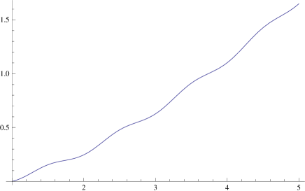
As we see from the Figure 2, for $n\gg 1$, the exponents $d_{n}\rightarrow 0.3n\ln n$ independent of magnitude of a constant $C$ meaning that at least in this limit the scaling exponents are universal.

Summary and Conclusions. 1. This paper is based on equations (6)-(8) leading to the well-defined Gaussian low-order moments of velocity derivatives and increments. In this case, “Strong Turbulence “ is defined as a first appearance of anomalous scaling exponents of the moments of the dissipation rate. No inertial range enters the considerations.
2. In the spirit of Landau’s theory of transition, it is assumed that in each statistical realization the transition occurs at $\hat{R}_{\lambda,n}\geq 9.$, independent on $n$. The numerical value of transitional Reynolds number $R_{\lambda}\approx 8.908$ was derived in Refs.[14]-[16]. Also, this result comes out of semi-empirical theories of large-scale turbulence modeling (Ref.[16]).
3. As follows from this paper, these two very strong dynamic constraints are satisfied by formation of small-scale coherent structures leading to intermittency (anomalous scaling) of dissipation fluctuations in turbulence.
4. The universality of these results is yet to be studied. On one hand, recently it has found some support in numerical and experimental data on various flows [9],[17],[18]. On the other hand, as we see from Table.1, numerical values of exponents $d_{n}$ may be sensitive to statistics of the low-Reynolds number fluctuations.
One argument in favor of broad universality can be found in Ref[11], (Model C), where dynamic renormalization group was applied to the problem of the Navier-Stokes equations driven by various random forces. The authors considered a general force (6) of an arbitrary statistics, supported in a finite interval of wave-numbers $k\approx k_{f}$ and showed that in the limit $k<<k_{f}$ the velocity fluctuations, generated by the model, obeyed Gaussian statistics. This result can be readily understood: each term of the perturbation expansion of (6)-(8) is $O(k^{2n})$. Therefore, in the limit $k\rightarrow 0$, all high-order contributions with $n>1$ disappear as small. This situation corresponds to weak coupling. It is not yet clear how universal this result is.
5. The relation (16) for anomalous exponents $d_{n}$ is a consequence of the coupling of dissipation rate and the random fluctuations of transitional Reynolds numbers (coupling constant) studied in Ref. [1]. The present paper is the first where the role of randomness of a transition point itself in the dynamics of small-scale velocity fluctuations has been addressed. It may be of interest to incorporate this feature in the field-theoretical approaches, like Wyld’s diagrammatic expansions applied to the Navier-Stokes equations for small-scale fluctuations.
6. In this paper anomalous exponents of moments of velocity derivatives and those of dissipation rate have been calculated without introducing any adjustable parameters. Given tremendous success of large-scale engineering simulations [16] , [19], which evolved into an indispensable design tool, we tend to conclude that Nelkin’s question,“ In What Sense Turbulence is Unsolved Problem?”, posed almost 25 years ago, may need be discussed again.