Improved Spectral Clustering for Multi-Objective Controlled Islanding of Power Grid

Abstract

We propose a two-step algorithm for optimal controlled islanding that partitions a power grid into islands of limited volume while optimizing several criteria: high generator coherency inside islands, minimum power flow disruption due to teared lines, and minimum load shedding. Several spectral clustering strategies are used in the first step to lower the problem dimension (taking into account coherency and disruption only), and CPLEX tools for the mixed-integer quadratic problem are employed in the second step to choose a balanced partition of the aggregated grid that minimizes a combination of coherency, disruption and load shedding. A greedy heuristic efficiently limits search space by generating starting solution for exact algorithm. Dimension of the second-step problem depends only on the desired number of islands $K$ instead of the dimension of the original grid. The algorithm is tested on standard systems with $118$, $2383$, and $9241$ nodes showing high quality of partitions and competitive computation time.

1 Introduction

A power grid is a complex technical system; hence, it is prone to technical disturbances. Even direct losses from infrastructure damage and blackouts are enormous, so, much attention is paid to assuring system sustainability under probable external and internal shocks. Controlled islanding is the process of splitting an interconnected power grid into smaller electrically independent parts. It is used as a last-resort effort to cope with many technical disturbances including undamped oscillations, voltage collapse, cascading trips, etc. ahmed2003scheme ; sun2003ImbalancecoherenceOBDD .

The rationale behind the process of controlled islanding is that a smaller grid is easier to stabilize: islands have not be synchronized, low frequency oscillations are less likely to occur in a small grid, and so on. Also, the islanding operation can isolate ill parts of the system from healthy ones, and the blackout will be localized at ill islands if not avoided.

So, controlled islanding is a last chance to keep the grid alive (at least, partially), which is a desirable effect. But there are also some side effects.

First of all, controlled islanding requires a series of complex actions performed with high accuracy and coordination. Any error can cause a cascading trip of generators or transmission lines.

Secondly, some power transmission lines are switched off during the islanding operation, which makes a great shock to the grid even when islanding is accurately planned and perfectly implemented. Such disruption leaves a partitioned grid in a highly unstable state, making it questionable to stabilize the state of some islands. The simplest metrics of the power flow disruption is the total volume of power flows broken during an islanding operation.

Thirdly, a well-designed interconnected grid has more opportunities to serve the current demand than any partitioned grid due to limited power transmission and ramp rate opportunities of the latter. Therefore, some load shedding is an essential part of the controlled islanding process junchen2015CoherencyDisruptionImbalanceCompare .

After all, restoring the grid after the controlled islanding is also a time-consuming and complex operation.

Bearing in mind high risks of controlled islanding, it is important to plan properly the islanding operation and to suggest a realistic and safe grid partitioning scheme that will stabilize the grid and minimize side effects.

Optimal islanding of a real-world power system is a high-dimensional optimization problem. The islanding decision is made under the extremal time pressure; a system operator has just several seconds to develop and implement an islanding scheme. Therefore, finding an optimal grid partition becomes a non-trivial task.

Metrics of system stability considered by power system security studies are computationally expensive. Shocks incurred by islanding operation must be classified as large-scale, and non-linear effects cannot be neglected. Hence, to make reliable predictions of the after-islanding system dynamics extensive time-domain simulations are performed under the paradigm of transient stability analysis kundur2004StabilitySurvey .

That is why most formal models of optimal controlled islanding (OCI) do not consider directly restoring system stability as an optimization criterion. Workarounds include incorporating external constraints (e.g., limited island volume) or constructing some simpler criteria, e.g., degree of generators’ coherency (or dynamic coupling) in the pre-islanding system state. Many articles leave stability constraints behind the scene (e.g., ding2013CoherencyDisruptionConstrainedSpectralBisection ; quiros2014determination ; sanchez2014AdmittanceDisruptionHierSpec ; trodden2014optimization and many others) concentrating on minimization of side effects of the islanding process, and most of them take into account only a single aspect (load shedding in fanpardalos2012SLDC_MILP ; pahwa2013ShedLoadDCGreedy ) or a couple of aspects (e.g., generator coherency and flow disruption in ding2013CoherencyDisruptionConstrainedSpectralBisection ).

A mathematical model of OCI introduced in the present article takes into account multiple aspects of the islanding process and their corresponding performance metrics (generator coherency chow1987Sparsetimescale , flow disruption li2005strategic , load shedding, and, optionally, line susceptance). A fast and efficient two-step algorithm is proposed to calculate a rational scheme of partitioning a grid into the desired number of islands $K$ with the limited maximum island volume.

In the first step hierarchical spectral clustering algorithms from sanchez2014AdmittanceDisruptionHierSpec ; quiros2015constrained are used to break the grid into $n^{\prime}>K$ islands to minimize the weighted combination of coherency and flow disruption metrics.

In the second step each of detailed grid partitions obtained in the first step is transformed into the aggregated grid with $n^{\prime}$ vertices. The aggregated grid is then partitioned into $K$ connected islands with the limited maximum island volume by an exact algorithm implemented in CPLEX 12. A greedy heuristics provides an efficient starting solution, which sufficiently fosters calculations. In addition to generator coherence and flow disruption the optimization criterion in the second step also takes into account the power imbalance inside islands.

The idea is to combine high speed (as the problem dimension is efficiently reduced in the first step) and high flexibility (complex optimization criteria and constraints are allowed in the second step). Computational experiments on the models of standard power systems with 118, 2383, and 9241 nodes show that the proposed algorithm is fast enough and outperforms alternative approaches both in bulk and in the value of every single performance metric.

The rest of the article has the following structure. In Section 2 recent approaches to OCI are surveyed. Then in Section 3 we introduce the notation and basic mathematical concepts used to define controlled islanding performance metrics. In Section 4 essential information is provided about spectral clustering, which is the main tool for fast and efficient islanding. The two-step algorithm for multi-objective grid partitioning is introduced in Section 5, while computational experiments on three cases of power grids are presented in Section 6. Section 7 concludes with some open issues and perspectives.

2 Literature Review

After a critical breakdown (e.g., a shortage, a circuit trip, or a generator failure) a power grid may become instable. Different groups of generator go out of sync, and the main goal of the automated grid control is to return the system into the stable state with minimum load shedding. In ahmed2003scheme ; vittal1998FirstStabilityManual it is shown that controlled islanding (accompanied with appropriate load shedding) can be a promising strategy to prevent cascading blackouts in power systems. A sort of modal analysis (analysis of normal forms) was employed in vittal1998FirstStabilityManual to perform generators’ grouping while in ahmed2003scheme predefined islands were considered. At the same time, the choice of a rational grid partitioning strategy was a challenging discrete optimization problem. System stability and the amount of load shedding were considered as the main criteria of partition quality.

Shed load is the amount of load that cannot be served safely given the topology of islands in the grid according to voltage and safety constraints and, thus, should be disconnected during the islanding operation. Shed load can be obtained by solving the optimal load shedding (OLS) problem under the alternating current (AC) model. AC-OLS reduces to a non-linear optimization problem pahwa2013ShedLoadDCGreedy , which takes sufficient time to solve. A simpler version of OLS problem often used in contingency analysis is the direct current (DC) approximation, which reduces to the linear program with (real) power flow balance, phase angle and maximum real flow constraints pahwa2013ShedLoadDCGreedy .

Even in a small power grid the number of alternative islanding schemes is enormous. An operator has just few seconds to choose and implement a grid islanding scheme (e.g., some generators go out of step within 5 sec after the contingency in the scenario modeled in xu2010SimplifyMETIS ). A detailed time-domain simulation cannot be run for every alternative partition to verify its stability, and indirect stability indicators are typically used at the partition selection stage (a notable exception is the use of PSSENG time-domain simulation in the genetic algorithm elWerfelli2008StabilityGenetic to evaluate island stability of IEEE 118-bus scheme).

A popular stability indicator of an electrical power system is coherency of its generators you2004CoherencySimulation (their aspiration to swing together). Generator grouping methods based on slow coherency detection were primarily developed for system model reduction chow1987Sparsetimescale ; chow1988Twotimescale ; chow1991Twotimescale . Several approaches were proposed (see chow1995CoherencyGreedy ; yusof1993Coherency ) to construct complete grid partitions by assigning loads to generator groups, but they ignored load shedding and the other metrics relevant to controlled islanding (e.g., transmission line security constraints).

In  sun2003ImbalancecoherenceOBDD ; zhao2003ImbalancecoherenceOBDDpostprocessing controlled islanding is considered as a satisfiability problem (the problem of finding a grid partition that fulfills a set of constraints). Ordered binary decision diagrams (OBDD) were used for limited enumeration of islanding schemes that satisfy generator coherency and load/generation balance constraints, while DC-OLS is run for each candidate solution until stability constraints are verified. OBDD-based enumeration is time-demanding, so large real-world networks have to be aggregated before applying the algorithm.

Load shedding is minimized in pahwa2013ShedLoadDCGreedy by solving a series of DC-OLS problems inside a greedy algorithm. Stochastic programming is used in golari2014stochastic ; golari2016large to find an islanding scheme, which minimizes the average load shedding against a series of pre-defined contingencies. In fanpardalos2012SLDC_MILP ; trodden2013milp ; trodden2014optimization ; ding2015SLMILP the grid partitioning problem is reduced to the mixed-integer linear program (MILP) with additional generator coherency constraints in trodden2013milp ; trodden2014optimization ; ding2015SLMILP and connectivity constraints in ding2015SLMILP . MILP is solved with exact algorithms implemented in CPLEX numeric optimization package. Nevertheless, computational experiments on grids with $\leq 300$ nodes show that these algorithms are time expensive and, hence, hardly applicable to online islanding problems.

To improve time efficiency of algorithms the amount of load shedding is often approximated by the load/generation imbalance. In particular, a heuristic algorithm is proposed in wang2004ImbalanceCoherenceHeuristic to minimize total load/generation imbalance under generator coherency constraints, but its time and cost efficiency was not compared to alternative approaches.

In addition to generator coherency, the power flow disruption is another popular indicator of the island (in)stability li2005strategic ; peiravi2009fast . When a transmission line is tripped during an islanding operation, the power flow through this line immediately drops to zero. The greater is the disruption (total power flow through the lines being teared), the greater is the excessive shock to the islanded power system (in addition to the initial disturbance) and the less possible is its stabilization.

Algorithms of controlled islanding based on spectral clustering techniques are intensively studied in recent years. The idea of using spectral clustering techniques for fast partitioning of electrical networks can be traced back to li2005strategic ; yang2007UnclearSpectral . A Spectral Clustering Controlled Islanding (SCCI) scheme is proposed in ding2013CoherencyDisruptionConstrainedSpectralBisection . It accounts both for generator coherency and power flow disruption. In the first step the normalized spectral bisection is used to divide the generators in two coherent groups. In the second step loads are assigned to generator groups using the unnormalized constrained spectral bisection to minimize the flow disruption. Recursive bisection is applied to obtain the desired number of islands. SCCI algorithm is shown to be much faster than OBDD-based enumeration techniques zhao2003ImbalancecoherenceOBDDpostprocessing ; sun2003ImbalancecoherenceOBDD with the minor loss in solution quality.

Later this methodology was extended in different aspects. In particular, $k$-medoids algorithm is used to cluster eigenvector points ding2014constrained instead of $k$-means suggested in li2005strategic . The problem of outliers when performing eigenvector analysis is addressed in ding2014constrained . Recursive bisection were replaced by direct $k$-way partitions in ding2014constrained ; sanchez2014AdmittanceDisruptionHierSpec , which decreased computation cost and increased partition quality.

In sanchez2014AdmittanceDisruptionHierSpec it is proposed to incorporate hierarchical clustering algorithm (first introduced in ward1963hierarchical ) into the spectral clustering scheme to stimulate generation of connected islands. In quiros2015constrained this approach is extended to account for generator coherency. Predefined generator groups are considered and loads are assigned to the nearest neighboring generator in the same spectral graph embedding. Finally, in quiros2014determination the spectral clustering approach is applied to the problem of parallel system restoration, which differs from controlled islanding in several important aspects.

An essential limitation of OCI algorithms based on spectral clustering is their disregard of load shedding. A yet another serious gap is that spectral methods sometimes result in extremely imbalanced partitions (those consisting of a huge mainland and several tiny islets), which is not practical in many ways.

The present article is devoted to further development of the spectral approach to OCI. We overcome existing shortcomings by using the hierarchical spectral clustering algorithms from sanchez2014AdmittanceDisruptionHierSpec ; quiros2015constrained as pre-processing routines to decrease the problem dimensionality to the desired degree caring only for generator coherency and flow disruption. Island volumes and shed load are accounted for in the second step of the proposed algorithm, where mixed-integer quadratic problem (MIQP) is solved.

3 Basic Notation

Every islanding decision is unique, since it is made under unique (and often unexpected) conditions. The state of the power system at the moment before the islanding decision is described by several groups of variables. Table 1 summarizes the notation used to define the context of an islanding process and its performance metrics.

Let us consider a power grid consisting of $n$ nodes (so called, buses) indexed from 1 to $n$, and $m$ transmission lines. Without loss of generality assume that at most one generator or a load is assigned to each bus and all generators are located at the first $n_{g}\leq n$ buses. Bold is used for vectors.

Table 1: Nomenclature

Notation	Description
$N=\{1,...,n\}$	Set of buses in the grid
$N_{g}=\{1,...,n_{g}\}$	Set of buses with generators installed
$V_{i}$	Voltage amplitude at bus $i\in N$
$\theta_{i}$	Phase angle at bus $i\in N$
$G_{i}$	Maximum real power output of generator at bus $i\in N_{g}$
$g_{i}$	Current real power output of generator at bus $i\in N_{g}$
$D_{i}$	Real power demand at bus $i\in N$
$d_{i}$	Current real load at bus $i\in N$
$p_{i}=d_{i}-g_{i}$	Current real power injection at bus $i\in N$
$p(s)=\sum_{i\in s}p_{i}$	Load/generation imbalance in island $s\subseteq N$
$p_{ij}$	Current real power flow from bus $i\in N$ to bus $j\in N$, $i>j$,
	($p_{ij}<0$ if the flow is directed from $j$ to $i$)
$P=(p_{ij})_{i,j=1}^{n}$	Real power flow matrix (lower-triangular)
$\bar{p}_{ij}$	Real power flow limit for the line between buses $i,j\in N$
$H_{i}$	Inertia constant of machine at bus $i\in N_{g}$
$Y=(y_{ij})_{i,j=1}^{n}$	Nodal complex admittance matrix
$B=(b_{ij})_{i,j=1}^{n}$	Nodal susceptance matrix, $B=\operatorname{Im}(Y)=\left(\begin{array}[]{cc}B_{11}&B_{12}\\ B_{21}&B_{22}\\ \end{array}\right)$,
	where $B_{11}$ is $n_{g}\times n_{g}$ sub-matrix limited to generator buses only
$\Delta=(\Delta_{ij})_{i,j=1}^{n}$	Electrical distance matrix defined in cotilla2013multiGA on the basis of $B$ matrix
$\tilde{B}=(\tilde{b}_{ij})_{i,j=1}^{n_{g}}$	Reduced susceptance matrix butyrin2003 : $\tilde{B}=B_{11}-B_{12}B_{22}^{-1}B_{21}$
$\tilde{\Phi}=(\phi_{ij})_{i,j=1}^{n_{g}}$	Dynamic coupling matrix of generators ding2013CoherencyDisruptionConstrainedSpectralBisection ,
	where $\phi_{ij}=\left(\frac{1}{H_{i}}+\frac{1}{H_{j}}\right)|V_{i}||V_{j}|\tilde{b}_{ij}\cos(\theta_{i}-\theta_{j})$
$\Phi=\left(\begin{array}[]{cc}\tilde{\Phi}&0\\ 0&0\\ \end{array}\right)$	Dynamic coupling matrix ($n\times n$) of generator buses
$\mathbf{w}=(w_{i})_{i=1}^{n}$	The vector of bus volumes, where $\mathbf{w}=|P|\cdot\mathbf{1}_{n}$ (alternatively, $w_{i}=G_{i}+D_{i}$; another volume metric is also possible)
$w(s)=\sum_{i\in s}w_{i}$	Volume of island $s\subseteq N$

Let $\mathbf{1}_{n}$ be the $n$-dimensional all-ones vector, $\mathbf{0}_{n}$ be the $n$-dimensional all-zeros vector, and let $I_{n\times n}=\operatorname{diag}(\mathbf{1}_{n})$ be the $n\times n$ identity matrix. For real symmetric $n\times n$ matrix $A=(a_{ij})_{i,j=1}^{n}$ its Laplace matrix is defined as

$$L(A):=\operatorname{diag}(A\cdot\mathbf{1}_{n})-A.$$

of volumes $\mathbf{w}$ is also given (see Table 1 for possible definitions of $\mathbf{w}$), the symmetric normalized Laplace matrix of matrix $A$ under volumes $\mathbf{w}$ is defined as

$$L_{sym}(A|\mathbf{w}):=\operatorname{diag}(\mathbf{w})^{-\frac{1}{2}}\cdot L(A)\cdot\operatorname{diag}(\mathbf{w})^{-\frac{1}{2}}.$$

Power flows in a power grid are naturally modeled by a directed graph with weights assigned to its vertices (representing injections in buses) and to arcs (representing real power flows through transmission lines). Let us introduce the notion of the graph cut, which plays the central role throughout the article. Consider a simple directed graph with vertex set $N$ and arc weights $a_{ij}$, $i,j\in N$. For vertex set $s\subseteq N$ the cutset is the minimum set of arcs needed to be removed to isolate $s$ from the rest of the graph. The total weight of the cutset is called the cut, which is calculated as

$$Cut_{A}(s):=\sum_{i\in s,j\in N\backslash s}a_{ij}=x^{T}L(A)x,$$

where $A:=(a_{ij})_{i,j=1}^{n}$ is the matrix of arc weights, and $x$ is an indicatory vector of vertex set $s$ (i.e., $x_{i}=1$ if vertex $i\in s$, and $x_{i}=0$ otherwise).

An islanding scheme with $K$ islands is represented by partition $\pi=(s_{1},...,s_{K})$ of vertex set $N$ into $K$ disjoint parts. For partition $\pi=(s_{1},...,s_{K})$ the cut is defined as

$$Cut_{A}(\pi):=\sum_{k=1}^{K}Cut_{A}(s_{k})=\operatorname{tr}X^{T}L(A)X,$$

where $X$ is $n\times K$ indicatory matrix of partition $\pi$ (i.e., $x_{ik}$ is equal to unity when $i\in s_{k}$ and is zero otherwise).

For positive vector $\mathbf{w}=(w_{i})_{i=1}^{n}$ of vertex volumes the normalized cut is defined as

$$NCut_{A}(\pi|\mathbf{w}):=\sum_{k=1}^{K}\frac{Cut_{A}(s_{k})}{w(s_{k})}=\operatorname{tr}Z^{T}L_{sym}(A|\mathbf{w})Z,$$ (1)

where $w(s):=\sum_{i\in s}w_{i}$ is the volume of island $s\subseteq N$, $Z=\operatorname{diag}(\mathbf{w})^{\frac{1}{2}}X\operatorname{diag}(X^{T}\mathbf{w})^{-\frac{1}{2}}$ (in the other words, $z_{ik}=\sqrt{\frac{w_{i}}{w(s_{k})}}$ if $i\in s_{k}$ and is zero otherwise.) Matrix $Z$ is orthogonal, i.e., $Z^{T}Z=I$.

Many popular performance metrics of controlled islanding can be written in terms of a graph cut with appropriately weighted graph arcs. For any $K$-partition $\pi=(s_{1},...,s_{K})$ generators’ dynamic coupling is defined in ding2013CoherencyDisruptionConstrainedSpectralBisection as

$$C(\pi)=Cut_{\Phi}(\pi),$$ (2)

and power flow disruption is defined as

$$D(\pi)=Cut_{|P|}(\pi).$$ (3)

Here the absolute power flow matrix (nonnegative and symmetric) is defined as $|P|:=(\frac{1}{2}|p_{ij}|+\frac{1}{2}|p_{ji}|)_{i,j=1}^{n}$, where $p_{ij}$ is the real power flow along arc $ij$.

In the present article we follow ding2013CoherencyDisruptionConstrainedSpectralBisection and use dynamic coupling matrix $\Phi$ (defined in Table 1) to build metric (2) of generator coherence. Alternatively, more sophisticated approaches (e.g., independent component analysis ariff2013coherency or hierarchical trajectory cluster analysis juarez2011characterization ) can be employed to build another matrix of generators’ coherence, which can be used in $C(\pi)$.

The electrical cohesiveness index (ECI), defined as

$$ECI(\pi):=Cut_{\Delta}(\pi),$$

was used in cotilla2013multiGA to split the grid on the basis of electrical distance matrix $\Delta$.

The shed load is the amount of load that cannot be served safely given the topology of islands in the grid according to voltage and safety constraints. For partition $\pi=(s_{1},...,s_{K})$ the shed load is denoted as

$$S(\pi):=\sum_{k=1}^{K}S(s_{k}),$$

where $S(s_{k})$ is the load shed in island $s_{k}$. Several approaches with different accuracy and computational complexity are used to evaluate $S(s_{k})$. Let $S_{AC}(s_{k})$ be the amount of load shedding in island $s_{k}$ in the solution of AC-OLS. Since AC-OLS is computationally expensive, below we calculate it only for final partitions to verify the quality of the solution.

DC-OLS is a simpler version of OLS problem limited to real flows with fixed bus voltages, zero line losses, and low phase angle differences. DC-OLS reduces to the linear program with real power flow balance, phase angle and maximum real flow constraints pahwa2013ShedLoadDCGreedy . The load shed in island $s_{k}$ calculated from OLS-DC solution is denoted by $S_{DC}(s_{k})$.

The estimate of shed load calculated as a solution of the maximum flow problem for island $s_{k}$ obtained by relaxing phase angle constraints in DC-OLS, is denoted as $S_{MF}(s_{k})$ (see more details in Section 5.4 below). Finally, when maximum real flow constraints are relaxed, the minimum amount of shed load is estimated by excess load:

$$S_{EL}(s_{k}):=\max\left[p(s_{k});0\right],$$ (4)

where $p(s):=\sum_{i\in s}(d_{i}-g_{i})$ is total imbalance between load $d_{i}$ and generation $g_{i}$ in nodes $i\in s$ of island $s\subseteq N$. If losses in lines are neglected, then $p(s_{k})=Cut_{P}(s_{k})$, where $P=(p_{ij})_{i,j=1}^{n}$ is a matrix of real power flows, and excess load is also expressed using the (directed) graph cut.

Finally, we note that $S_{EL}(s)\leq S_{MF}(s)\leq S_{DC}(s)\leq S_{AC}(s)$ for any island $s\subseteq N$, so AC-OLS gives the most conservative estimate of the shed load.

4 Spectral Clustering Basics

Spectral clustering is an approach to finding approximate solutions of minimum cut problems for weighted undirected graphs. Consider an undirected simple graph $\langle N,E\rangle$ with vertex set $N=\{1,...,n\}$, edge set $E\subseteq N\times N$, and non-negative edge weights $a_{ij}$, $ij\in E$. Then, given matrix $A=(a_{ij})_{i,j=1}^{n}$ (non-negative and symmetric), the graph minimum $K$-cut (or $K$-partition) problem is to find a partition $\pi=(s_{1},...,s_{K})$ of a vertex set $N$ into $K$ disjoint parts that minimizes $Cut_{A}(\pi)$.

If, in addition, positive volume $w_{i}$ is assigned to every vertex $i\in N$, the minimum balanced $K$-cut problem is to minimize $Cut_{A}(\pi)$ by choosing a partition $\pi=(s_{1},...,s_{K})$, such that $w(s_{k})\leq W,k=1,...,K$, where $W\geq W(N)/K$ is an upper cluster volume limit.

The minimum $K$-cut problem is known goldschmidt1988polynomial to be solvable in polynomial time $O(n^{K^{2}})$ for any fixed $K$, but is NP-complete GareyJohnson1979 when $K$ is not limited. The minimum balanced cut problem is NP-complete GareyJohnson1979 even for the graph bipartition problem (when $K=2$, $n$ is even, $w_{i}=1$, and $W=n/2$).

Many efficient approximate graph partitioning algorithms were developed since then, with spectral clustering being among most popular ones. For spectral clustering the balanced $K$-cut problem is replaced with $NCut_{A}(\pi|\mathbf{w})$ minimization problem with no cluster volume constraints resulting is some sort of relaxation: for partition $\pi=(s_{1},...,s_{K})$

$$NCut_{A}(\pi|\mathbf{w})=\frac{Cut_{A}(s_{1})}{w(s_{1})}+...+\frac{Cut_{A}(s_{K})}{w(s_{K})},$$ (5)

and denominators in (5) penalize small cluster volumes, while for equal cluster volumes (such that $w(s_{1})=...=w(s_{K})$) we have

$$NCut_{A}(\pi|\mathbf{w})=Cut_{A}(\pi)\cdot\frac{K}{w(N)}.$$

Spectral clustering is based on the spectral lower bound for the trace minimization problem lutkepohl1996handbook . For an arbitrary real symmetric $n\times n$ matrix $A$ let $\lambda_{i}(A)$, $i=1,...,n$, be its eigenvalues enumerated in ascending order, and let $\mathbf{u}_{i}(A)$ be corresponding eigenvectors. Then for any $n\times K$ orthogonal matrix $Z$, $K\leq n$, the following inequality holds:

$$\operatorname{tr}Z^{T}AZ\geq\lambda_{1}(A)+...+\lambda_{K}(A)=\operatorname{tr}U^{T}AU,$$ (6)

where $U=(\mathbf{u}_{1}(A),...,\mathbf{u}_{K}(A))$ is a matrix composed of $K$ first (normalized) eigenvectors of matrix $A$.

Any $K$-partition can be written in the form of an orthogonal $n\times K$ binary matrix $X=(x_{ik})$, where $x_{ik}=1$ if an only if $i$-th node belongs to $k$-th cluster. Spectral clustering algorithms approximate expression $\operatorname{tr}U^{T}AU$ in (6) with some admissible partition $X$, which is close in some sense to matrix $U$. The convenient notation is developed below for basic algorithms of spectral clustering, which is used in the next section to build combined partitioning algorithms.

According to equation (1), the normalized cut is written with normalized Laplace matrix $L_{sym}(A|\mathbf{w})$, so in the classical algorithm ng2002spectral the rows of matrix $U$, whose columns are the first $K$ eigenvectors of $L_{sym}(A|\mathbf{w})$, are normalized to the unit Euclidian norm and then partitioned with $k$-means clustering. Each row corresponds to a graph vertex. Denote the resulting $K$-partition with $\kappa_{K}(A|\mathbf{w})$.

The algorithm of $k$-means is known to be sensitive to outliers (arising, for example, when graph has pendent vertices). It is shown in demetriou2013implementing that more stable islanding schemes for real power grids can be obtained when $k$-means is replaced with the more robust $k$-medoids algorithm. The corresponding partition is denoted with $\mu_{K}(A|\mathbf{w})$.

Both $k$-means and $k$-medoids often suggest disconnected subgraphs as partition elements. To deal with with problem it is suggested in sanchez2014AdmittanceDisruptionHierSpec to use hierarchical clustering instead. In the Hierarchical Spectral Clustering (HSC) algorithm sanchez2014AdmittanceDisruptionHierSpec the graph is pre-processed by iteratively merging pendent vertices to their neighbors. No pendent vertex are left in the graph to avoid the outlier problem. Then eigenvector matrix $U$ is calculated for the normalized Laplacian of the absolute power flow matrix $|P|$. Normalized rows of matrix $U$ are considered as points on a $K$-dimensional sphere and the graph being partitioned is embedded onto this sphere. The distance between any pair of graph vertices is calculated as the length of the shortest path in the embedded graph (the cosine distance between incident nodes is considered). A hierarchical clustering algorithm ward1963hierarchical is then applied to the obtained distance matrix (Standard Matlab implementation with complete linkage defays1977efficient is used below.) The shortcoming of this algorithm is bigger variation of island volumes: a partition often consists of one or two big islands and a collection of small islets. Let $\chi_{K}(|P|~{}|\mathbf{w})$ stand for the $K$-partition built with hierarchical normalized spectral clustering.

Let us consider a simplistic numeric example by partitioning a tiny power grid (the IEEE 9-bus system shown in Figure 1) by HSC algorithm. The network has 3 generators installed, 3 loads and the total of 9 buses. The (outbound) real power flows, current real power generations and loads calculated using AC-OPF are presented in Figure 1 with arrows showing the flow direction. To calculate a bisection of this network with HSC algorithm, pendent nodes 1,2, and 3 are joined respectively to nodes 4,7, and 9. The matrix of absolute power flows for the resulting 6-nodal graph is

$$|P|=\left(\begin{array}[]{cccccc}0&27.15&17.60&0&0&0\\ 27.15&0&0&36.05&0&0\\ 17.60&0&0&0&0&27.45\\ 0&36.05&0&0&30.95&0\\ 0&0&0&30.95&0&19.10\\ 0&0&27.45&0&19.10&0\\ \end{array}\right),$$

and matrix

$$U=\left(\begin{array}[]{cc}-0.4603&-0.0075\\ -0.2665&0.3019\\ -0.4708&0.7119\\ -0.2808&-0.0240\\ -0.5631&-0.5882\\ -0.3155&-0.2355\end{array}\right)$$

stores the two smallest eigenvectors of its normalized Laplacian.

Each diamond or cross on the unit circle in Figure 2(a) represents some row of matrix $U$ additionally normalized to the unit norm. Each point corresponds to a graph node (their numbers are listed in the figure with generator nodes marked with the star), and connecting the points with graph edges (bold curves in the figure) we obtain the spectral graph embedding. Every edge is labelled with a weight being equal to the distance on the circle between its ends. The dendrogram of the hierarchical clustering applied to the weighted distance matrix of this graph is also shown in Figure 2(a). The root of the dendrogram is located at zero, and the smaller dashed circle in Figure 2(a) shows the level, at which exactly two clusters are separated. The nodes of the first cluster are denoted with diamonds, while the nodes of the second one are denoted with crosses. It is worth noting that since we use graph distances, node $1,4^{*}$ is closer to node $5$ than to node $8$ (which can also be seen at the dendrogram).

The resulting islanding scheme is presented in Figure 2(b), which shows teared lines and equilibrium post-islanding generations, power flows, and loads (the shares of demand served are shown in frames). Islanding performance metrics are also presented: generator coherence $C$, disruption $D$ and shed load $S$ (according to AC-OPF model).

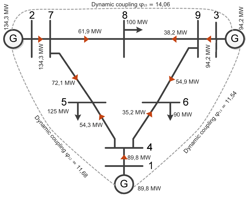
Figure 1: Example of pre-islanded network and power flows

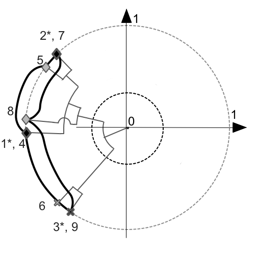
(a) Spectral graph embedding and the dendrogram for HSC

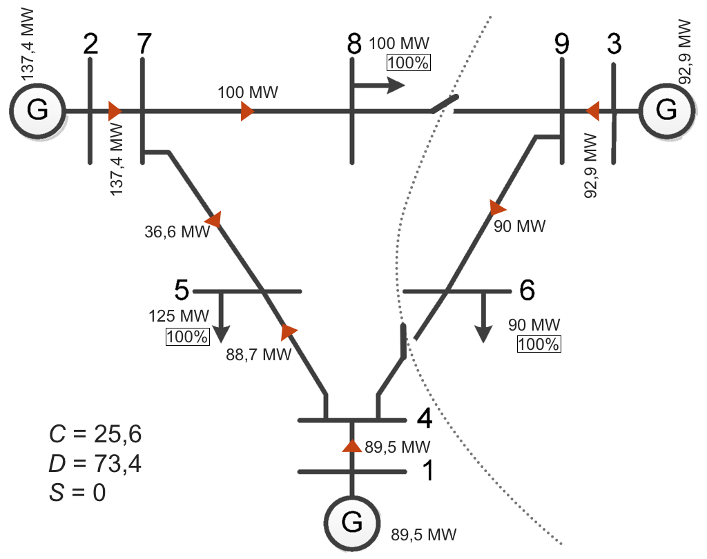
(b) Post-islanded network, power flows and islanding performance metrics

Figure 2: An illustration of HSC algorithm

In many applications it is important to keep some pairs of vertices in different clusters (e.g., generators with low dynamic coupling) and the other pairs should always be assigned to a single cluster (e.g., highly coupled generators). The algorithm of constrained spectral clustering bie2004constrainedclustering uses projection matrix technique to generalize the spectral clustering approach to the case of such must-link and cannot-link constraints, but it can be applied only for graph bisection (for $K=2$). Constrained spectral clustering is used in ding2013CoherencyDisruptionConstrainedSpectralBisection ; ding2014constrained ; quiros2015constrained to control coherent generator groups. In the first step of SCCI algorithm ding2013CoherencyDisruptionConstrainedSpectralBisection the dynamic graph with set $N_{g}=\{1,...,n_{g}\}$ of generators and weights’ matrix $\tilde{\Phi}$ is considered and all generators are divided in two coherent groups using some spectral bisection algorithm. In the second step unnormalized constrained spectral clustering is used to select a bisection of grid graph that minimizes flow disruption and fulfills must-link and cannot-link constraints: generators from the same coherent group must go to one island while those from different groups cannot go to one island.

Therefore, the first two eigenvectors $\mathbf{u}_{1},\mathbf{u}_{2}$ of the generalized eigenvalue problem

$$H^{T}L(|P|)H\mathbf{u}=\lambda H^{T}H\mathbf{u}$$

are calculated, where $H$ is a projection matrix. If, without loss of generality, $s_{1}^{\prime}=\{1,...,n_{1}\}$, then

$$H=\left(\begin{array}[]{ccc}\mathbf{1}_{n_{1}}&\mathbf{1}_{n_{1}}&\mathbf{0}_{n_{1}}\\ \mathbf{1}_{n_{g}-n_{1}}&-\mathbf{1}_{n_{g}-n_{1}}&\mathbf{0}_{n_{g}-n_{1}}\\ \mathbf{1}_{n-n_{g}}&\mathbf{0}_{n-n_{g}}&I_{(n-n_{g})\times(n-n_{g})}\\ \end{array}\right).$$

After that the rows of matrix $U=(\mathbf{u}_{1},\mathbf{u}_{2})$ are split in two clusters using the $k$-medoids algorithm. The same procedure should be applied recursively to the biggest island of the partition until the desired number of partitions is obtained.

Another Constrained Spectral Clustering (CSC) methodology of intentional controlled islanding is proposed in quiros2015constrained . CSC algorithm starts from predefined groups $s_{1}^{g},...,s_{K}^{g}\subseteq N_{g}$ of coherent generators (probably, identified with independent component analysis ariff2013coherency or hierarchical trajectory cluster analysis juarez2011characterization ) and aims at forming islands by distributing loads between these generator groups to minimize the normalized cut of absolute power flow matrix.

Analogously to HSC algorithm, $K$ first eigenvectors of the normalized Laplacian of absolute power flow matrix $|P|$ are used to calculate the graph embedding onto the $K$-dimensional unit sphere. As in HSC algorithm, the distance between a pair of graph vertices is evaluated as the length of the shortest path in the embedded graph (again, cosine distance between incident vertices is considered). Finally, the $K$-partition of the graph is built by assigning each vertex to the $i$-th island if and only if the nearest generator vertex in the embedded graph belongs to group $s_{i}^{g}$. Let us denote with $\sigma_{K}(|P|~{}|\mathbf{w},\pi^{g})$ a $K$-partition built by CSC algorithm given absolute power flow matrix $|P|$, partition $\pi^{g}=\{s_{1}^{g},...,s_{K}^{g}\}$ of generators into coherent groups, and vector $\mathbf{w}$ of bus weights.

To illustrate CSC algorithm, let us bipartition the 9-bus network (see Figure 1). The spectral graph embedding coincides with that of HSC algorithm (see Figure 3(a)). From Figure 1 we see that generators at buses $2$ and $3$ have higher dynamic coupling $\phi_{ij}$, so let us form the two generator groups: $\{1\}$ (denoted with the black cross in Figure 3(a)) and $\{2,3\}$ (denoted by two black diamonds in Figure 3(a)). Any other bus is assigned to the generator group being closest to this bus in the graph embedding (see the dashed arrows in Figure 3(a)). Two resulting islands, post-islanding power flows, and islanding performance metrics are presented in Figure 3(b). Load shedding at buses 5 and 6 is required to balance generation and load in the bigger island.

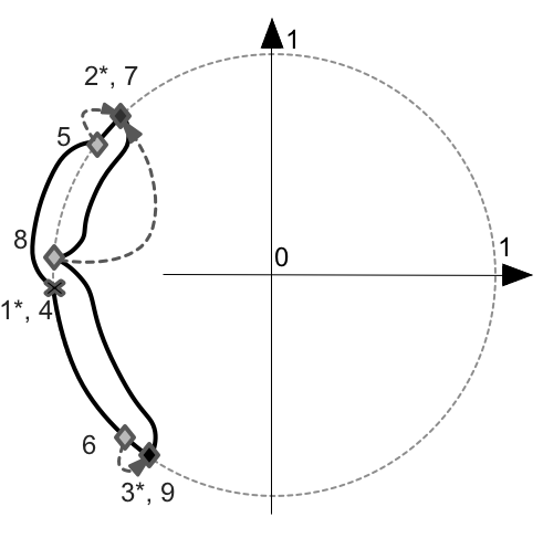
(a) Spectral graph embedding and load bus assignments for CSC

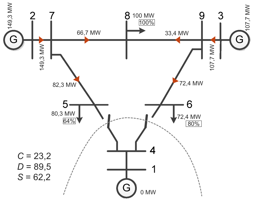
(b) Post-islanded network, power flows and islanding performance metrics

Figure 3: An illustration of CSC algorithm

Like SCCI, CSC algorithm takes care both of generator coherence and power flow disturbance, but CSC is shown in quiros2015constrained to work faster. At the same time, it disregards shed load (e.g., compare $S$ in Figures 2(b) and 3(b)). Also, under this methodology the size of islands being created is hardly controllable.

The goal of the present article is to improve spectral clustering algorithms of OCI (namely, HSC and CSC algorithms) by proposing a methodology, which flexibly accounts for generator coherence, power flow disruption, shed load, and island sizes.

The deeper insight into spectral clustering techniques can be found in von2007tutorial ; sanchez2014AdmittanceDisruptionHierSpec ; quiros2014determination and in the references provided by these articles.

5 Improved Spectral Clustering Algorithm

5.1 Problem Setting

Effect of islanding criterion on the stability of the islanded grid was analyzed in junchen2015CoherencyDisruptionImbalanceCompare . An experiment with IEEE 118-bus scheme has shown that an islanding scheme with minimum power flow disruption is the most stable one; the scheme with minimum excess demand results in considerably lower load shedding at the cost of longer relaxation time, while under a coherency-based islanding scheme, which ignores disruption and imbalance, generators fail to stabilize.

It is not clear at the moment to what extent these observations generalize to other contingency cases and to other power grids: different performance metrics may be valuable predictors of island stability in different situations. Therefore, a universal algorithm of OCI should combine multiple criteria (generator coherency, power flow disruption, some metric of load shedding, minimum or maximum island volume, and others) and their relative importance should be flexibly adjusted.

Distinct to numerous approaches to OCI that consider preserving generator coherence as a primary optimization goal and calculate coherent generator groups in advance using the two-time-scale theory chow1987Sparsetimescale ; chow1988Twotimescale ; chow1991Twotimescale or recent approaches ariff2013coherency ; juarez2011characterization , below the slow coherency detection technique from ding2013CoherencyDisruptionConstrainedSpectralBisection is adopted and dynamic coupling $C(\cdot)$ is included into the optimization criterion along with other performance metrics. OCI is considered as a multi-objective optimization problem: to find a $K$-partition $\pi=(s_{1},...,s_{K})$ of grid graph $\langle N,E\rangle$ that minimizes the weighted sum of multiple metrics

$$F(\pi)=\alpha_{C}C(\pi)+\alpha_{D}D(\pi)+\alpha_{ECI}ECI(\pi)+\alpha_{S}S(\pi)$$ (7)

and has the limited maximum island volume:

$$w(s_{k})\leq W,k=1,...,K.$$ (8)

The proper choice of weights is discussed in the last section.

Without loss of generality assume $\alpha_{S}=1$. Then $F(\pi)$ can be written as

$$F(\pi)=Cut_{A}(\pi)+S(\pi),$$ (9)

where

$$A=(a_{ij})_{i,j=1}^{n}:=\alpha_{C}\Phi+\alpha_{D}|P|+\alpha_{ECI}\Delta.$$ (10)

If shed load is estimated using the maximum flow approximation (see the previous section), OCI reduces to choosing $x_{ik}\in\{0,1\}$, $z_{ij}\in\{0,1\}$, $y_{ij}\in\left[-\bar{p}_{ij}z_{ij},\bar{p}_{ij}z_{ij}\right]$, $l_{i}\in[0,D_{i}]$, $g_{i}\in[0,G_{i}]$ for $i\in N$, $k=1,...,K$, $ij\in E$ to

minimize $$\operatorname{tr}X^{T}L(A)X+\sum_{i=1}^{n}l_{i}$$ (11)

subject to constraints:

island volume $$\sum_{i=1}^{n}w_{i}x_{ik}\leq W \forall k=1,...,K,$$

nodal flow balance $$D_{i}-l_{i}=g_{i}+\sum_{j:ji\in E}y_{ji}-\sum_{j:ij\in E}y_{ij} \forall i=1,...,n,$$

islands’ detachment $$\sum_{k=1}^{K}k(x_{ik}-x_{jk})\leq K(1-z_{ij}),$$

$$- \sum_{k=1}^{K}k(x_{ik}-x_{jk})\leq K(1-z_{ij}) \forall ij\in E,$$

vertex partitioning $$\sum_{k=1}^{K}x_{ik}=1 \forall i=1,...,n.$$

Here $X=(x_{ik})$ is an $n\times K$ indicatory matrix of the grid partition, so that $x_{ik}=1$ if and only if bus $i$ belongs to island $k$, $y_{ij}$ is a real power flow through line $ij\in E$ (limited by the maximum flow $\bar{p}_{i}j$), $z_{ij}=1$ if and only if line $ij\in E$ lies inside a single island (and, thus, is not switched off when the grid is partitioned), $l_{i}$ and $g_{i}$ are, correspondingly, shed load volume and real power output at bus $i\in N$, while $D_{i}$ and $G_{i}$ being, respectively, real power demand and maximum real power output of generator at bus $i$.

Since the Laplace matrix is always positively semidefinite, the problem in hand is convex MIQP with $nK+m$ binary and $2n+m$ real variables. Nevertheless, numeric optimization packages (e.g., CPLEX) cannot be applied directly to this problem due to its high dimension. Below an efficient computational approach is introduced that avoids the combinatorial explosion.

5.2 Idea of Algorithm

Matrix $A$ in expression (10) is symmetric and non-negative, so existing algorithms of spectral clustering can minimize $Cut_{A}(\pi)$, the first term of cost function (9). At the same time, distinct to the standard graph cut problem the sparsity pattern of matrix $A$ does not coincide with that of graph adjacency matrix due to coupling coefficients $\phi_{ij}$ that directly “connect” non-adjacent generator buses $i,j\in N_{g}$. As a result, the classical spectral clustering algorithm ng2002spectral often suggests disconnected islands with lots of generation-rich and generation-deficient connected components (and, hence, with poor load shedding). The connectivity problem can be avoided by using hierarchical spectral clustering sanchez2014AdmittanceDisruptionHierSpec that, in most cases, generates connected islands.

Absolute power flow matrix $|P|$ is included, among the others, into matrix $A$, so partition $\pi$ with low $Cut_{A}(\pi)$ typically has reasonably low flow disruption $D(\pi)$. In turn, disruption, to some extent, correlates with load shedding: when losses are neglected, the inequality

$$S_{EL}(s)=\max\left[Cut_{P}(s);0\right]\leq Cut_{|P|}(s)=D(s)$$

holds for any island $s\subseteq N$, which means that low disruption implies low excess load (but not vice versa, in general). So, when looking for the partition that minimizes a combination of load shedding and disruption, one can limit attention to partitions with relatively low disruption.

We use this observation to propose the Improved Spectral Clustering (ISC) algorithm of controlled islanding. In the first step of the algorithm a limited set of partitions is obtained with low $Cut_{A}(\cdot)$, while in the second step a partition that minimizes $Cut_{A}(\cdot)+S_{MF}(\cdot)$ is selected from this set (load shedding is estimated using the maximum flow model). To detect more candidate partitions, in the first step different spectral clustering techniques are combined to build several alternative graph $rK$-cuts, where $r>0$ is some granularity factor. Then, in the second step, some of $rK$ islands are merged to obtain a $K$-partition that minimizes $Cut_{A}(\cdot)+S_{MF}(\cdot)$.

The following story illustrates the idea of the algorithm. Imagine someone has a porcelain plate with flowers painted on it (see Fig. 4(a) and wants to divide it into four pieces of roughly equal size keeping flowers unbroken. To obtain such pieces a plate can be sawed carefully (one of possible solutions is shown in Fig. 4(b) but it is extremely time-consuming. Instead, one can break a plate into small pieces with a strong hammer blow and then glue some pieces back to compose as much entire flowers as possible. Although the latter approach may result in a suboptimal solution (e.g., five flowers are broken in Fig. 4(c)), it is much faster and can be the only alternative when time is expensive.

Details of the algorithm are explained in the next two subsections.

(a) Initial plate

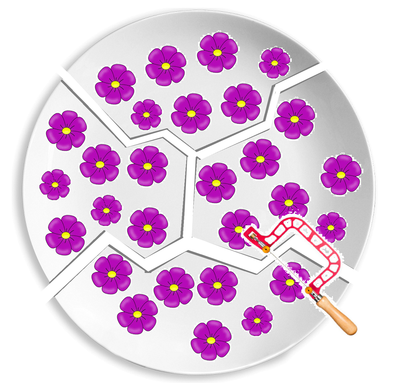
(b) Saw plate

(c) Broken plate

Figure 4: An illustration of the idea of the algorithm

5.3 Step 1: Spectral Clustering

Below we simplify presentation by assuming that $\alpha_{ECI}=0$ in (7). To apply normalized spectral clustering, the balanced cut problem with maximum cluster volume constraints is replaced with the corresponding minimum normalized cut problem without cluster volume constraints. Seven different strategies are used in parallel in the first step to build overdetailed partitions. Then, in the second step of the algorithm, each of these partitions is rolled up into a $K$-partition.

1. Fixed-granularity strategy for matrix $A$. Granularity factor $r_{1}>1$ (which is a tunable parameter of the algorithm) is chosen and $r_{1}K$-partition $\pi^{\text{\ref{strategy_fixedA}}}:=\chi_{r_{1}K}(A|\mathbf{w})$ of the grid is built with HSC algorithm sanchez2014AdmittanceDisruptionHierSpec .

2. Fixed-granularity strategy for matrix $|P|$. It has already been noted that low disruption implies low excess load, so partitions with low $D(\cdot)$ seem more likely to minimize cost function (7) than those with low $C(\cdot)$. Therefore, partition $\pi^{\text{\ref{strategy_fixedP}}}:=\chi_{r_{2}K}(|P|~{}|\mathbf{w})$ is computed, where granularity factor $r_{2}>1$ is a yet another tunable parameter.

3. Minimum-granularity strategy for matrix $A$. From inequality (6) it follows that exactly $K$ Laplacian eigenvectors are enough to characterize a $K$-partition with small normalized cut. So, overdetailed partitions in Strategies I and II are forced by the need to satisfy volume constraints (8) and to leave some combinatorial space for the shed load optimization. Instead, in Strategy III a partition $\pi^{\text{\ref{strategy_minA}}}:=\chi_{K^{\prime}}(A|\mathbf{w})$ is chosen with minimum granularity $K^{\prime}\in\{K,...,r_{1}K\}$ that satisfies cluster volume constraints (8) (i.e., if $s\in\pi^{\text{\ref{strategy_minA}}}$ then $w(s)\leq W$).

4. Minimum-granularity strategy for matrix $|P|$. Similarly to the previous strategy, we choose the partition $\pi^{\text{\ref{strategy_minP}}}:=\chi_{K^{\prime\prime}}(|P|~{}|\mathbf{w})$ with minimum granularity $K^{\prime\prime}\in\{K,...,r_{2}K\}$ that satisfies cluster volume constraints (8).

5. Minimum-granularity-refined CSC algorithm. CSC algorithm minimizes disruption under given groups of coherent generators. In our methodology selection of coherent generator groups on the basis of dynamic coupling $\Phi$ (or alternative generator coherence metric) is a part of the optimization process. In Strategy V coherent generator groups for CSC algorithm are calculated by HSC algorithm applied to reduced dynamic coupling matrix $\tilde{\Phi}$. Consequently, $\pi^{\text{\ref{strategy_CSC}}}:=\sigma_{K^{\prime\prime\prime}}(|P|~{}|\chi_{K^{\prime\prime\prime}}(\tilde{\Phi}|\mathbf{w}),\mathbf{w})$ for the minimal granularity $K^{\prime\prime\prime}\in\{K,r_{3}K\}$ that allows to satisfy island volume constraints (8) (as before, $r_{3}>0$ is a tunable parameter).

6. Fixed-granularity sequential strategy for $|P|$ and $A$. HSC algorithm generates a partition $\chi_{K}(|P|~{}|\mathbf{w})$ that has low disruption but neglects generator coherency. So, recursive bisection for graph edge weights’ matrix $A$ is applied to partition $\chi_{K}(|P|~{}|\mathbf{w})$ to obtain more granulated $r_{4}K$-partition (again, $r_{4}>1$ is a tunable parameter), which combines low disruption and coherency.

   Let us denote with $\nu(\sigma,\pi|\mathbf{w})$ a partition obtained from partition $\pi$ by splitting island $s\in\pi$, which has the biggest volume $w(s)$, with a bisection procedure $\sigma$. Define

   $$\nu_{K}(\sigma,\pi|\mathbf{w})=\nu(\sigma,\nu(...,\nu(\sigma,\pi|\mathbf{w})|...)|\mathbf{w})$$

   a partition being a result of $K$ recursive bisections $\nu$ of the initial partition $\pi$. Then, $\pi^{\text{\ref{strategy_fixedPA}}}:=\nu_{(r_{4}-1)K}(\chi_{2}(A|\mathbf{w}),\chi_{K}(|P|~{}|\mathbf{w})|\mathbf{w})$. The idea behind this strategy is that we never miss low-disruption partition $\chi_{K}(|P|~{}|\mathbf{w})$ and potentially can improve by joining islands in another order in the second step of the algorithm.

7. Crossing CSC and HSC partitions. CSC algorithm builds a partition $\sigma_{K}(|P|~{}|\chi_{K}(\tilde{\Phi}|\mathbf{w}),\mathbf{w})$ focusing mainly on generator coherence. On the contrary, HSC algorithm constructs a partition $\chi_{K}(|P|~{}|\mathbf{w})$ caring only for flow disruption. A finer partition $\pi^{\text{\ref{strategy_meet}}}:=\sigma_{K}(|P|~{}|\chi_{K}(\tilde{\Phi}|\mathbf{w}),\mathbf{w})\wedge\chi_{K}(|P|~{}|\mathbf{w})$ is obtained as a meet of these two partitions in the aggregation lattice. Set $s\subseteq N$ belongs to the meet if an only if $s=s_{1}\cap s_{2}$ for some $s_{1}\in\sigma_{K}(|P|~{}|\chi_{K}(\tilde{\Phi}|\mathbf{w}),\mathbf{w})$ and $s_{2}\in\chi_{K}(|P|~{}|\mathbf{w})$.

We limit ourselves to the above seven strategies, although other approaches to granulated partition construction are also possible.

5.4 Step 2: Partitioning Aggregated Grid

In the second step of the algorithm the granulated partition is transformed into $K$-partition by fusing some islands together. Each of detailed partitions $\pi^{\text{\ref{strategy_fixedA}}},...\pi^{\text{\ref{strategy_meet}}}$ is processed separately and, probably, in parallel.

First of all, all connected components of islands in partition $\pi^{i}$ are detached making separate islands. Let $\pi=(s_{1},...,s_{n^{\prime}})$ be the resulting detailed partition where each island is connected ($n^{\prime}>K$).

An aggregated grid is built such that each island $s_{k}$ in $\pi$ becomes its vertex with:

$$\begin{array}[]{rl}\text{maximum real power output}&G_{k}^{\prime}:=\sum_{i\in s_{k}}G_{i},\\ \text{current real power output}&g_{k}^{\prime}:=\sum_{i\in s_{k}}g_{i},\\ \text{real power demand}&D_{k}^{\prime}:=\sum_{i\in s_{k}}D_{i},\\ \text{current real power load}&d_{k}^{\prime}:=\sum_{i\in s_{k}}d_{i},\\ \text{injection}&p_{k}^{\prime}:=p(s_{k}),\\ \text{volume}&w_{k}^{\prime}:=w(s_{k}).\\ \end{array}$$

Also, for all island pairs $k,k^{\prime}=1,...,n^{\prime}$ define

$$\begin{array}[]{rl}\text{aggregated real power flows}&p_{kk^{\prime}}^{\prime}=\sum_{i\in s_{k},j\in s_{k^{\prime}}}p_{ij},\\ \text{real power limits}&\bar{p}_{kk^{\prime}}^{\prime}=\sum_{i\in s_{k},j\in s_{k^{\prime}}}\bar{p}_{ij},\\ \text{dynamic coupling coefficients}&\phi_{kk^{\prime}}^{\prime}=\sum_{i\in s_{k},j\in s_{k^{\prime}}}\phi_{ij}.\\ \end{array}$$

Edge $kk^{\prime}$ is included into edge set $E^{\prime}$ of the aggregated grid if $\bar{p}_{kk^{\prime}}^{\prime}>0$. Let $m^{\prime}:=|E^{\prime}|$ be the edge count of the aggregated grid, $m^{\prime}\leq n^{\prime}(n^{\prime}-1)/2$.

OCI problem (11) for the aggregated grid is a relaxation of the same OCI problem for the original power grid, because it replaces a group of detailed constraints for vertices of one island with a lump-sum constraint for the island as a whole. The aggregated grid problem is MIQP with $Kn^{\prime}+m^{\prime}$ binary and $2n^{\prime}+m^{\prime}$ real variables. Its dimension depends on the dimension of the aggregated grid but not on the dimension of the original grid, and if granularity $n^{\prime}$ of partition $\pi$ is small enough, this problem can be solved in eligible time using exact algorithms implemented in commercial numeric solvers (we use CPLEX 12.6.2.0).

If there are too many disconnected islands in $\pi^{i}$, dimension $n^{\prime}$ of the aggregated grid can still be too high for exact algorithms. In this case we suggest decreasing its dimension with the following greedy heuristics.

At each iteration this heuristics simplifies the partition by joining a pair of adjacent islands to minimize cost function (9) while fulfilling island volume constraints. The shed load in (9) is estimated with the excess demand $S_{ED}(\cdot)$:

$$F_{ED}(\pi):=Cut_{A}(\pi)+S_{ED}(\pi)=Cut_{A}(\pi)+\sum_{s\in\pi}\max[p(s),0].$$ (12)

The pseudo code is presented in Listing 1.

Listing 1 Greedy heuristic algorithm for OCI

1:function GreedyPartition($Grid$, $K$) $\triangleright$ cuts graph $Grid$ into $K$ parts

2:     with Grid

3:         $\pi\leftarrow\bigcup_{i\in N}\{i\}$ $\triangleright$ start from the finest partition

4:     end

5:     while $|\pi|>K$ do $\triangleright$ until requested island count is reached

6:         $\pi\leftarrow\operatorname{Argmin}\{F_{ED}(\pi^{\prime})~{}|\pi^{\prime}\in\textsc{Coarsen}(\pi),\pi^{\prime}=\textsc{ConnectedComponents}(\pi^{\prime})\}$

7:     end while

8:     return $\pi$

9:end function

10:

11:function Coarsen($\pi$) $\triangleright$ all admissible partitions obtained by fusing two islands in $\pi$

12:     return $\{\pi^{\prime}~{}|~{}\pi^{\prime}=\{\{s\cup s^{\prime}\}\}\cup(\pi\backslash\{s\}\backslash\{s^{\prime}\})\text{ for some }s,s^{\prime}\in\pi,w(s\cup s^{\prime})\leq W\}$

13:end function

The $K$-partition calculated by this greedy heuristics is also used as a record in the exact partitioning algorithm of the aggregated grid.

Finally, ISC algorithm selects the partition with the lowest cost of MIQP solution for seven aggregated grid built on the basis of partitions $\pi^{\text{\ref{strategy_fixedA}}},...,\pi^{\text{\ref{strategy_meet}}}$.

The pseudo code of ISC algorithm is presented in Listing 2.

Listing 2 Improved Spectral Clustering algorithm for OCI

1:function ImprovedSpectralPartition($Graph,K$)

2:     with $Graph$ $\triangleright$ assignments can be done in parallel

3:         $\pi^{\text{\ref{strategy_fixedA}}}\leftarrow\chi_{r_{1}K}(A|\mathbf{w})$

4:         $\pi^{\text{\ref{strategy_fixedP}}}\leftarrow\chi_{r_{2}K}(|P|~{}|\mathbf{w})$

5:         $K^{\prime}\leftarrow\min\left\{k=K,...,r_{1}K:s\in\chi_{k}(A|\mathbf{w})\Rightarrow w(s)\leq W\right\}$

6:         $\pi^{\text{\ref{strategy_minA}}}\leftarrow\chi_{K^{\prime}}(A|\mathbf{w})$

7:         $K^{\prime\prime}\leftarrow\min\left\{k=K,...,r_{2}K:s\in\chi_{k}(|P|~{}|\mathbf{w})\Rightarrow w(s)\leq W\right\}$

8:         $\pi^{\text{\ref{strategy_minP}}}\leftarrow\chi_{K^{\prime\prime}}(|P|~{}|\mathbf{w})$

9:         $K^{\prime\prime\prime}\leftarrow\min\left\{k=K,...,r_{3}K:s\in\sigma_{k}(|P|~{}|\chi_{k}(\tilde{\Phi}|\mathbf{w}),\mathbf{w})\Rightarrow w(s)\leq W\right\}$

10:         $\pi^{\text{\ref{strategy_CSC}}}\leftarrow\sigma_{K^{\prime\prime\prime}}(|P|~{}|\chi_{K^{\prime\prime\prime}}(\tilde{\Phi}|\mathbf{w}),\mathbf{w})$

11:         $\pi^{\text{\ref{strategy_fixedPA}}}\leftarrow\nu_{(r_{4}-1)K}(\chi_{2}(A|\mathbf{w}),\chi_{K}(|P|~{}|\mathbf{w})|\mathbf{w})$

12:         $\pi^{\text{\ref{strategy_meet}}}\leftarrow\sigma_{K}(|P|~{}|\chi_{K}(\tilde{\Phi}|\mathbf{w}),\mathbf{w})\wedge\chi_{K}(|P|~{}|\mathbf{w})$

13:     end

14:     for ${i=\text{\ref{strategy_fixedA}},...,\text{\ref{strategy_meet}}}$ do $\triangleright$ iterations can be performed in parallel

15:         $\pi\leftarrow\textsc{ConnectedComponents}(\pi^{i})$

16:         $Graph^{\prime}\leftarrow\textsc{AggregatedGraph}(Graph,\pi)$

17:         if $|\pi|\geq K^{max}$ then $\triangleright$ if partition dimension is too high

18:              $\pi\leftarrow\textsc{GreedyPartition}(Graph^{\prime},K^{max})$ $\triangleright$ decrease dimension

19:              $Graph^{\prime}\leftarrow\textsc{AggregatedGraph}(Graph^{\prime},\pi)$

20:         end if

21:         $\pi_{0}\leftarrow\textsc{GreedyPartition}(Graph^{\prime},K)$ $\triangleright$ record for exact algorithm

22:         $[\pi^{\prime},Cost^{i}]\leftarrow\textsc{SolveMIQP}(Graph^{\prime},K,\pi_{0})$ $\triangleright$ exact solution with MIQP solver

23:         $\pi^{i*}\leftarrow\textsc{FullPartition}(\pi^{\prime})$ $\triangleright$ obtain $K$-partition of $Grid$ graph

24:     end for

25:     $j:=\operatorname{Argmin}_{i=\text{\ref{strategy_fixedA}},...,\text{\ref{strategy_meet}}}Cost^{i}$ $\triangleright$ the best calculated $K$-partition

26:     return $\pi^{j*}$

27:end function

5.5 Numeric Example

This subsection illustrates the proposed ISC algorithm by partitioning the 9-bus network (see Figure 1) to minimize the sum of dynamic coupling, flow disruption, and shed load (with unit weights). The desired number of clusters $K=2$ and granularity factor is set to $r_{i}=1.5,i=1,...,4$, so, strategies I, II, and VI in the first step of ISC algorithm try to partition the network into $3$ islands. Therefore, three eigenvectors are calculated, and the spectral graph embedding in Strategies I and II is three-dimensional. Strategy I is based on matrix $A$ (a linear combination of dynamic coupling matrix $\Phi$ and absolute power flow matrix $|P|$), while Strategy II relies solely on matrix $|P|$. Spectral embeddings for these strategies (see Figures 5(a) and 5(b) respectively) differ a bit, but hierarchical clustering of the nodes of the spectral embedding results in the same three islands $\{1,4,5\},\{2,7,8\}$, and $\{3,6,9\}$ outlined in Figures 5(a) and 5(b).

In the second step of the algorithm, MIQP (11) is solved for the 3-nodal aggregated network, and the resulting bipartition is equal to that calculated by HSC algorithm (see Figure 2(b)). In the considered example, Strategy IV (based on HSC algorithm) and Strategy V (based on CSC algorithm) work as explained in Section 4 above, and the resulting islanding schemes are shown in Figures 2(b) and 3(b) respectively.

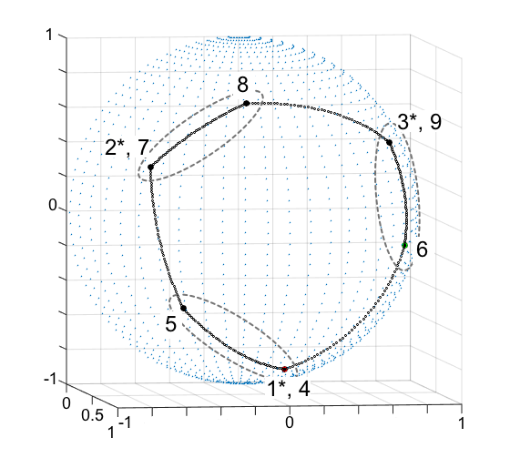
(a) Strategy I (for matrix $A$)

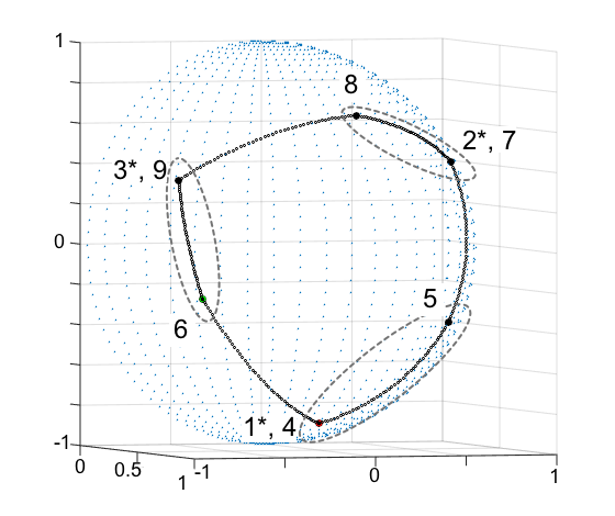
(b) Strategy II (for matrix $|P|$)

Figure 5: Spectral graph embedding and 3-cluster partitioning for Strategies I and II

The two-dimensional spectral embedding for Strategy III based on matrix $A$ is presented in Figure 6(a). The corresponding islanding scheme, post-islanding power flows, and islanding performance metrics are shown in Figure 6(b).

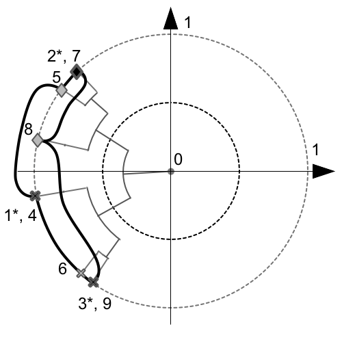
(a) Spectral graph embedding and the dendrogram

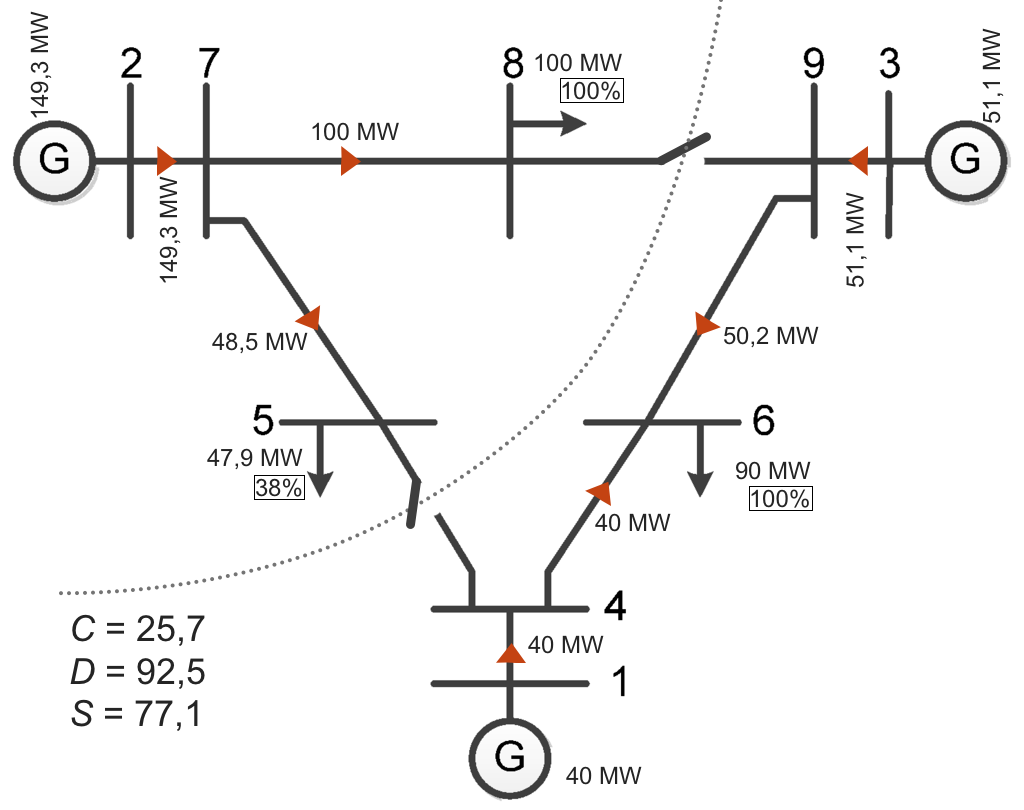
(b) Post-islanded network, power flows and islanding performance metrics

Figure 6: Steps of ISC algorithm: Strategy III

Strategy VI starts with the $K$-partition of the network generated by HSC algorithm (see Figure 2(a)) and sequentially bisects the biggest island using CSC algorithm until $r_{4}K$ islands are obtained. The three resulting islands are encircled by dotted lines in Figure 7(a). In Strategy VII we meet partitions generated by HSC algorithm (the dotted line in Figure 7(b)) and CSC algorithm (the dashed line in Figure 7(b)) and obtain three islands: $\{1,4\}$, $\{2,5,3,8\}$, and $\{3,6,9\}$. In the second step of the algorithm, MIQP (11) is solved for the corresponding aggregated 3-nodal networks, and the resulting partitions coincide with that shown in Figure 2(b) both for Strategies VI and VII.

Finally, the islanding scheme with the minimum cost is selected from the three distinct schemes (those shown in Figures 2(b), 3(b), and 6(b)) obtained by running two steps of ICS algorithm for Strategies I-VII.

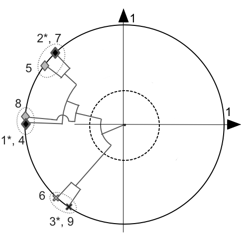
(a) Strategy VI: using CSC algorithm for sequential granulation of $\chi_{K}(|P|~{}|\mathbf{w})$

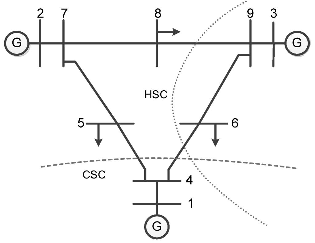
(b) Strategy VII: the meet of partitions generated by HSC and CSC

Figure 7: ISC algorithm: Strategies VI and VII

6 Performance Evaluation

6.1 Experimental Setup

Three test systems from MATPOWER 5.1 Simulation Package library zimmerman2011matpower were used to evaluate performance of the proposed ISC algorithm (see Table 2). These relatively big systems was taken to verify computational efficiency of ISC algorithm and its applicability to bulky real-world grids.

Table 2: Test power systems

Notation	Power system	Buses	Generators	Lines
SMALL	IEEE 118-bus test system IEEE118	118	54	186
MEDIUM	Polish system, winter peak 1999-2000 case2383wp	2383	327	2896
LARGE	European system (PEGASE project) fliscounakis2013contingency	9241	1445	16049

For each of three considered power systems 100 test cases were generated by switching off 5 random generators, breaking 5 random lines, and multiplying all demands by a random factor from 1 to 2. For every case consistent power flows were calculated by solving AC-OLS problem with opf routine of MATPOWER 5.1 zimmerman2011matpower for dispatchable loads.

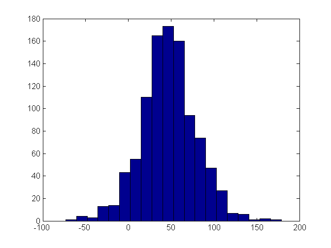
(a) Density of power flow from bus 37 to 34

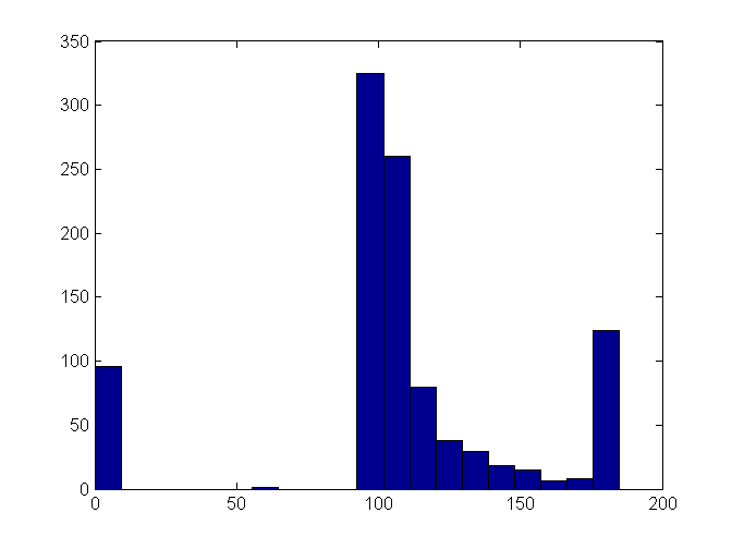
(b) Density of real power output at bus 12

Figure 8: Examples of power flow variables’ variation for 100 cases in SMALL system

These power flows and corresponding generators’ angles were used to calculate stability indicators (power flow disruption $D(\cdot)$ and dynamic coupling $C(\cdot)$) when an islanding operation is planned. Information on generator inertia constants was not available, so equal inertia constants were assumed when coefficients of dynamic coupling $\phi_{ij}$ were calculated.

The sample line power flow and the sample real power output in SMALL grid are depicted in Figure 8. High variance of these variables shows that considered collection of cases represents a wide range of power flow conditions in a grid. Such massive durability testing of OCI algorithms under the broad variety of grid and flow conditions is rarely performed in the existing literature. The only known exception is hamon2015two , where partitioning algorithms were tested under 2000 different power flow conditions in SMALL system.

We did not perform transient stability analysis to verify system stability after islanding, as the main concern of ISC algorithm was to improve the partition quality for existing island stability indicators and their combinations. At the same time, although simplified metrics of load shedding (such as excess demand) were employed when an optimal islanding scheme was searched, for performance evaluation the AC-OLS model was applied to the system partitioned according to seven partitioning strategies of ISC algorithm.

Additional constraints were imposed when AC-OLS problem was solved for the islanded system: generators’ output was limited by the short-term ramp rate and previously shed load could not be restored in the process of islanding. So, controlled islanding always results in extra load shedding compared to the pre-islanding system state.

Dynamic coupling, power flow disruption, and shed load had equal weights $\alpha_{C}=\alpha_{D}=\alpha_{S}=1$ in the optimization criterion (7) of ISC algorithm. The requested island count $K=4$ was selected for all three systems and granularity factors were set to $r_{1}=...=r_{4}=4$, i.e., 16 islands were demanded when calculating detailed partitions. The maximum island volume was $W=\frac{3}{8}W(N)$. In particular, this means that any admissible partition with four connected islands has at least three big islands (those having the volume $\geq\frac{W(N)}{4}$).

6.2 Partitioning Quality

ISC is an approximate algorithm, and there are several possible sources of its inaccuracy that should be inspected.

Firstly, there may be the discrepancy between real objectives of controlled islanding (i.e., preserving the transient stability and preventing a blackout with minimum load shedding) and their representation in the model (7) (a combination of computationally efficient metrics). Although being critical for the final efficiency of an islanding technique, analysis of model adequacy falls beyond the scope of the present article, which concentrates on the existing OCI metrics.

Another important aspect is the method used to evaluate load shedding. The estimate $S_{AC}(\cdot)$ of the shed load volume calculated from AC-OLS model is assumed the most accurate one, but ISC algorithm employs its maximum-flow relaxation $S_{MF}(\cdot)$ to reduce the problem to MIQP (11). Large discrepancy between these metrics may sufficiently distort the optimization criterion.

Figure 9 shows the relation between $S_{MF}(s)$ and $S_{AC}(s)$ for islands met in optimal partitions of SMALL and MEDIUM powers systems. It can be seen from the figure that $S_{MF}(\cdot)$ correlates well with $S_{AC}(s)$ but systematically underestimates the latter. Also, there are numerous situations when $S_{MF}(s)=0$ while $S_{AC}(s)>0$.

Accuracy of $S_{AC}(\cdot)$ prediction can be improved sufficiently by considering a three-variate non-linear regression

$$\bar{S}_{AC}(s)=\max\left[S_{MF}(s)-aGR_{MF}(s)+bw(s),0\right],$$ (13)

where $a$ and $b$ are regression parameters (grid-dependent, in general), $w(s)$ is the volume of island $s$, while $GR_{MF}(s)$ is the generation reserve. The latter is calculated as $GR_{MF}(s):=\sum_{i\in s}\left(G_{i}-g_{i}^{*}(s)\right)$, where $G_{i}$ is the maximum real power output of generator bus $i\in s$ and $g_{i}^{*}(s)$ is its real power output in the solution of MF-OLS problem for island $s$.

For comparison, scattering plots (predicted value $\bar{S}_{AC}(s)$ vs exact value $S_{AC}(\cdot)$) of regression (13) under the best parameter values ($a=0.43,b=0.02$ for SMALL system and $a=0.97,b=0.04$ for MEDIUM system) are shown in Figures 10(a) and 10(b) respectively. Correlation is 0.92 with mean absolute error (MAE) 13.9 MW on the training set and is 0.94 with MAE 14.1 on the testing set for SMALL system. For MEDIUM system correlation is equal to 0.99 with MAE 39.2 MW on the training set and is equal to 0.98 with MAE 39.5 MW on the testing set.

To take advantage of the more accurate regression (13) only minor change in MIQP setting (11) is needed. It is enough to introduce the new non-negative continuous variables $\sigma_{k}\geq 0$, $k=1,...,K$, which satisfy inequality constraints

$$\sigma_{k}\geq\sum_{i=1}^{n}x_{ik}\left[l_{i}-a(G_{i}-g_{i})+bw_{i}\right],k=1,...,K$$

and define the new cost function

$$\operatorname{tr}X^{T}L(A)X+\sum_{k=1}^{K}\sigma_{k}.$$ (14)

The revised MIQP still has linear constraints and the convex cost function. Therefore, its complexity does not increase, while its solution accurately predicts the optimal value of the cost function

$$F(\pi)=\alpha_{C}C(\pi)+\alpha_{D}D(\pi)+\alpha_{S}S_{AC}(\pi)$$

in the considered test systems and is expected to meet application-specific accuracy requirements.

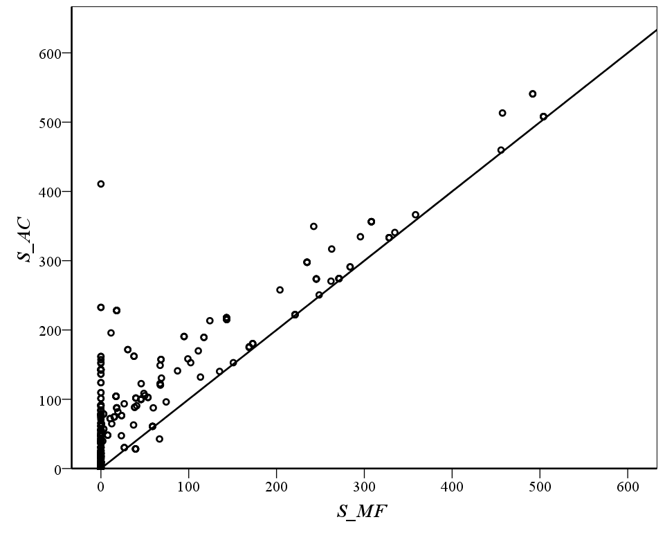
(a) SMALL system

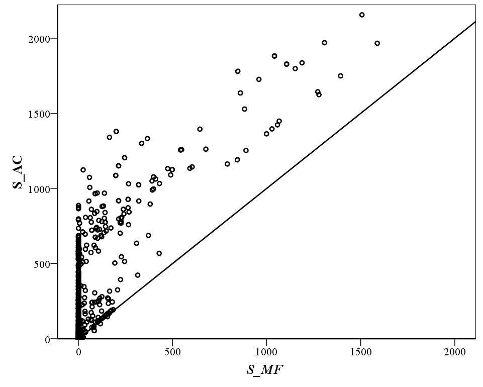
(b) MEDIUM system

Figure 9: Relation (scattering plot) between AC-OLS-based load shedding $S_{AC}(s)$ (vertical axis) and maximum-flow-based load shedding $S_{MF}(s)$ (horizontal axis). A diagonal line $y=x$ is added for clarity.

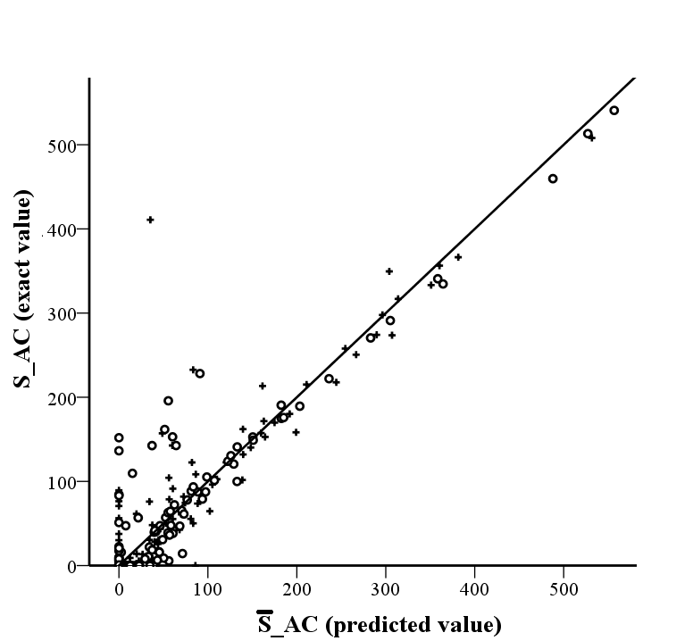
(a) SMALL system

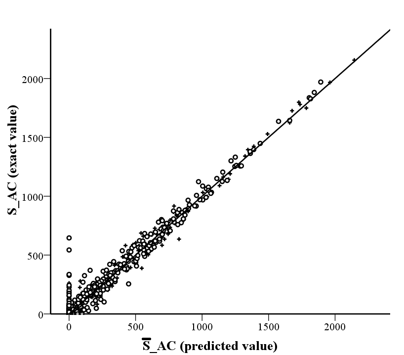
(b) MEDIUM system

Figure 10: Scattering plot for $S_{AC}(s)$ (vertical axis) and $\bar{S}_{AC}(s)$ (horizontal axis). Circles denote points of the training set, while pluses go for the testing set.

The final aspect of algorithm accuracy is that MIQP (11) is solved only approximately by ISC algorithm due to high problem dimensionality, and the approximation error of ISC algorithm should be estimated by comparing the ISC solution to the exact solution of MIQP (11). Due to computational intractability of problem (11) for large grids, such a direct error evaluation is impossible for MEDIUM and LARGE system, while for SMALL system the mean relative error of ISC algorithm for 100 cases is just $2\%$ (the maximum error is $9\%$). Therefore, approximation error is negligible.

Let us continue with algorithm benchmarking. The proposed ISC algorithm is based on CSC and HSC, the most efficient spectral-clustering-based algorithms for OCI. It is natural to use them as a benchmark in performance evaluation of ISC for large grids where exact solution is intractable. Unfortunately, $K$-partition $\chi_{K}(|P|~{}|\mathbf{w})$ computed by HSC algorithm is often imbalanced, and so does $K$-partition $\chi_{K}(\tilde{\Phi}|\mathbf{w})$, which we used to elicit coherent generator groups for CSC.

As a consequence, both CSC and HSC applied directly to our data in most cases return imbalanced partitions being highly impractical for controlled islanding. Figure 11 shows the volume of the largest island (relative to the total grid volume) for SMALL and MEDIUM test systems. The horizontal line shows the maximum volume constraint. HSC partitions are shown with circles, while crosses stand for CSC partitions. It follows from the figure that CSC returns a balanced partition only in 18 cases of 100 for SMALL system, while HSC results in a balanced partition in 12 cases. For MEDIUM system HSC returns a balanced condition just once, while CSC partitions are always imbalanced.

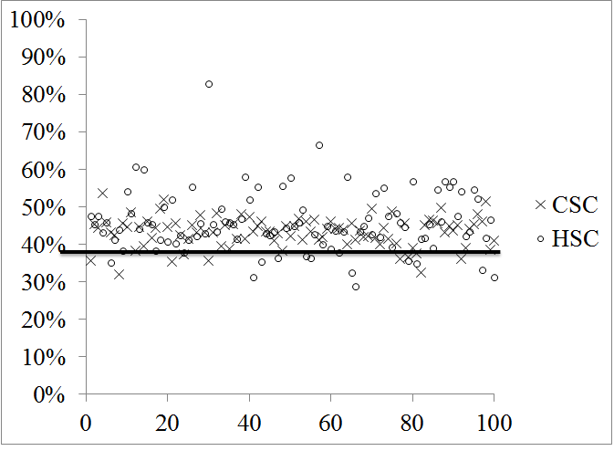
(a) SMALL system

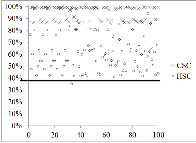
(b) MEDIUM system

Figure 11: Relative volume (per cent) of the largest island for $K$-partitions generated by CSC and HSC. Case numbers are depicted along the horizontal axis.

Win rates of seven strategies of ISC algorithm for three test systems are presented in Table 3. The winning strategy minimizes the cost function $F_{AC}(\cdot)$ with shed load evaluated from AC-OLS problem. Strategies VI and II appear the most successful for all three test systems, while Strategies IV and V only occasionally win (These strategies represent the closest balanced analog of HSC and CSC algorithms consequently, so they can be, to some extent, used as a baseline to compare ISC to the competing algorithms.)

Table 3: Win rate (per cent) of different strategies of ISC algorithms. Win rates of Strategies IV and V (separated by horizontal lines) can be used as a baseline for comparison of ISC with, respectively, HSC and CSC algorithms.

		Test power system
Strategy		SMALL	MEDIUM	LARGE
I	Fixed-granularity strategy for $A$	21	9	1
II	Fixed-granularity strategy for $|P|$	16	33	32
III	Minimum-granularity strategy for $A$	20	10	4
IV	Minimum-granularity strategy for $|P|$	3	4	14
V	Minimum-granularity refined CSC	0	2	3
VI	Sequential strategy for $|P|$ and $A$	29	37	38
VII	Crossing CSC and HSC partitions	11	5	8

The average partitioning quality of ISC algorithm for SMALL test system is depicted in Figure 12(a). The value of cost function is enclosed in a frame, all its components are also presented for all seven strategies and for the winning strategy. Although Strategy II (fixed granularity for matrix $|P|$) does not account directly for generator coherency, it suggests competitive coherency cost and wins in disruption and load shedding. At the same time, Strategy VI (sequential partitioning) has the same average cost due to a little bit lower generator coherency under a slightly higher disruption and shed load. These two strategies remain the leaders for all three test systems.

A yet another conclusion is that considering excessive number of eigenvectors (which is the main idea of ISC algorithm) is essential to achieve good performance, since Strategy IV, which differs from Strategy II only in the number of eigenvectors considered, is inferior. The same is true for Strategy V, which is based on CSC and also operates with the limited number of eigenvectors. Performance metrics of ISC strategies for MEDIUM system are presented in Figure 12(b).

The similar analysis for LARGE system is hindered by the fact that for this system some strategies often suggest imbalanced partitions (Strategies I, V, and VII show the worst success rate: 24% , 32%, and 34% respectively) even when $4K$ eigenvectors are calculated. Since island volume constraints are mandatory, ISC algorithm neglects imbalanced partitions suggested by some strategies when selecting the final solution, and there is no common base for the comparison of these strategies.

Therefore, maintaining several different partitioning strategies is important to always obtain a good islanding solution in large power systems.

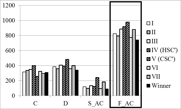
(a) SMALL system

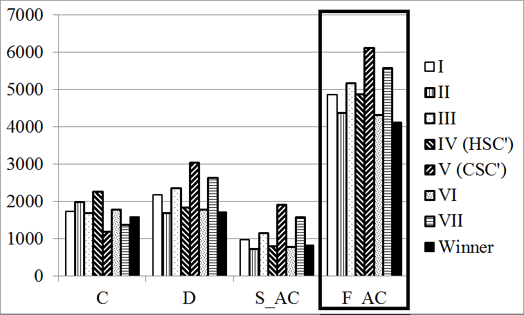
(b) MEDIUM system

Figure 12: Average performance metrics for Strategies I-VII of ISC algorithm. Total cost $F_{AC}(\cdot)$ is framed. Generator coherence $C(\cdot)$, flow disruption $D(\cdot)$, and shed load $S_{AC}(\cdot)$ are also shown.

6.3 Flexibility

In many existing OCI algorithms li2005strategic ; xu2010SimplifyMETIS ; ding2013CoherencyDisruptionConstrainedSpectralBisection ; sanchez2014AdmittanceDisruptionHierSpec ; quiros2015constrained an optimization criterion cannot be tuned to assign different importance to different performance metrics of controlled islanding. Distinct to them, in ISC algorithm the weights of cost function components (dynamic coupling, disruption, and shed load) can be chosen arbitrary leading to different resulting partitions. For example, in Figure 13 optimal islanding schemes for SMALL system under several extremal settings are presented. In Figure 13 weights in cost function (7) were chosen to minimize dynamic coupling $C(\cdot)$ while ignoring $D(\cdot)$ and $S(\cdot)$. On the contrary, in Figure 13 disruption $D(\cdot)$ is minimized with no attention paid to $C(\cdot)$ and $S(\cdot)$. The partition that balances generators’ dynamic coupling $C(\cdot)$ and disruption $D(\cdot)$ is presented in Figure 13, and the one taking care only for the shed load $S(\pi)$ is presented in Figure 13.

For comparison, the best alternative partition (calculated by HSC algorithm) and its performance metrics are presented in Figure 13. Therefore, every single performance metric of HSC partition or a combination of metrics can be improved by ISC algorithm, and the optimization criterion can be flexibly tuned to adjust relative importance of different metrics.

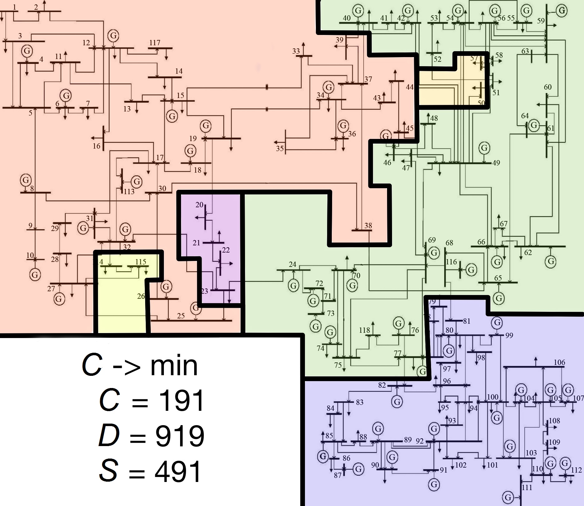
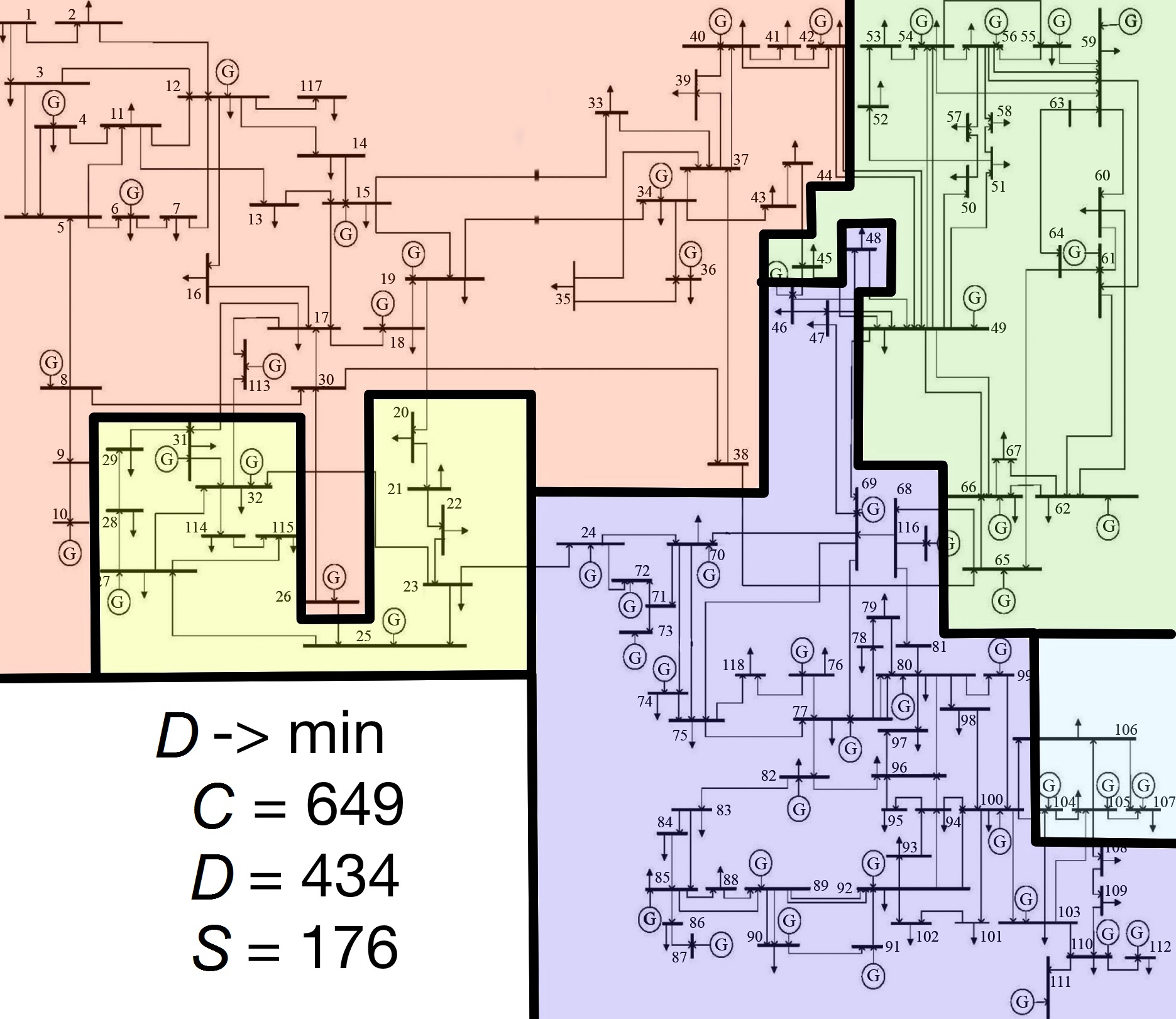
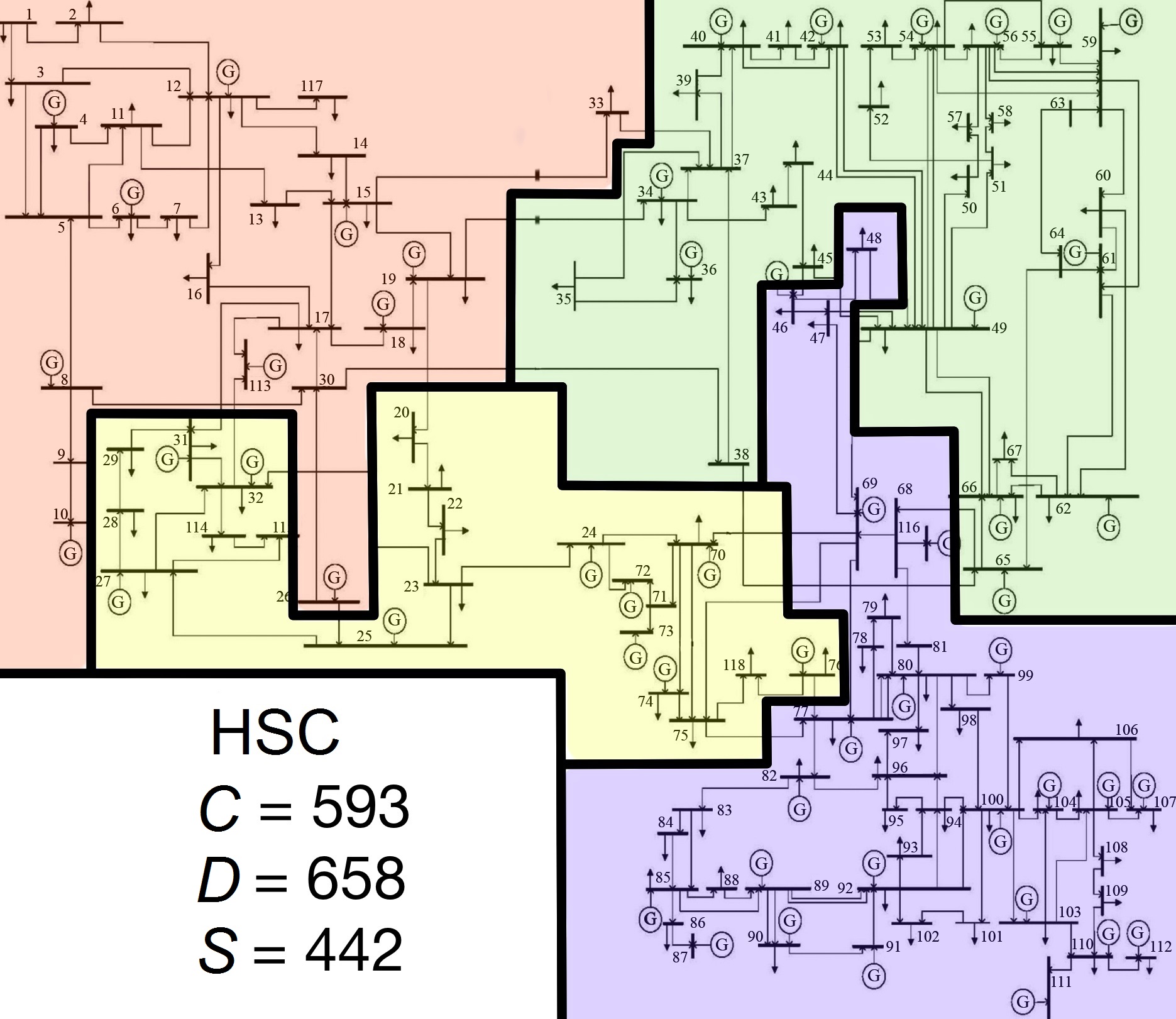
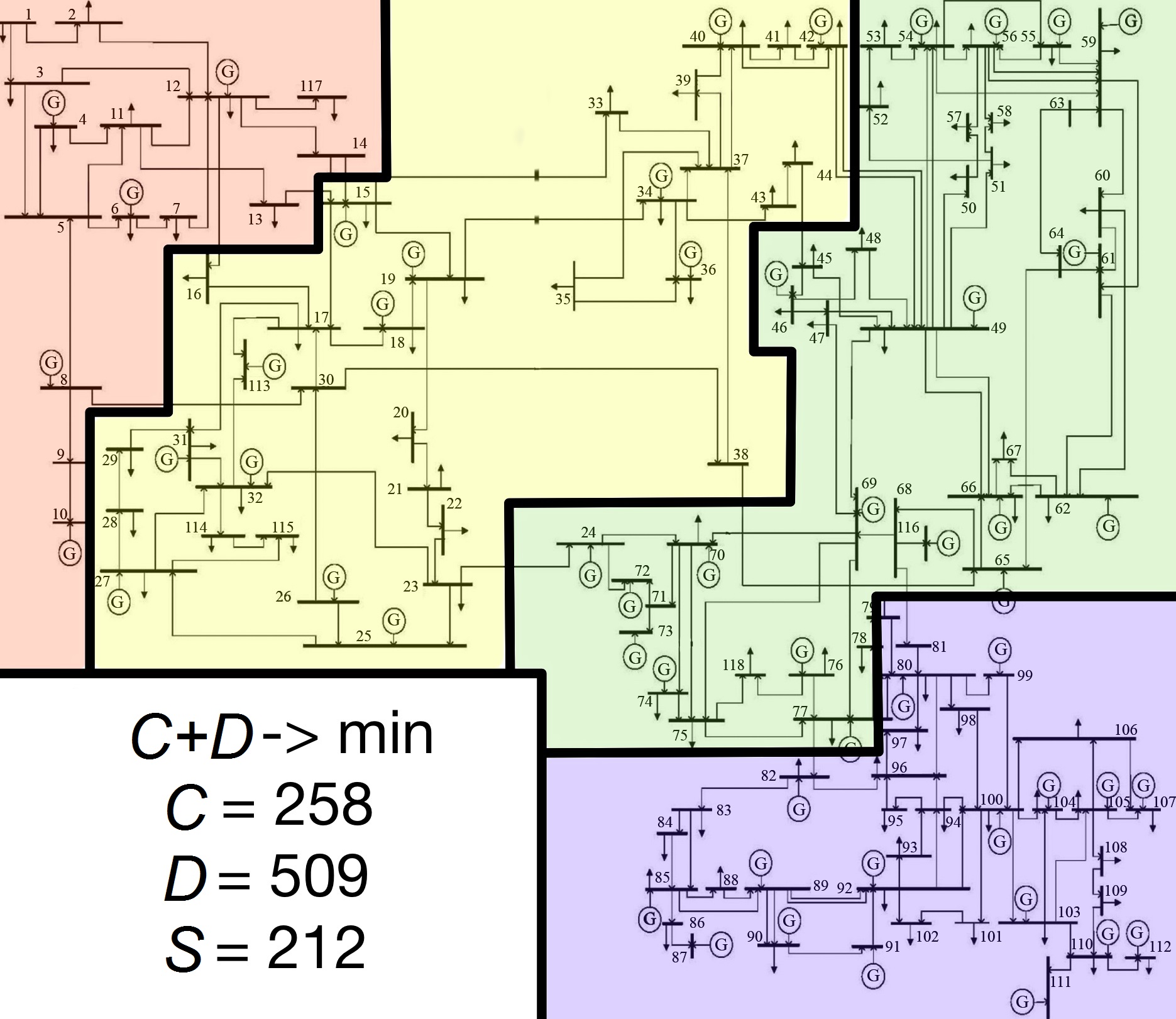
Figure 13: Optimal islanding schemes for different cost functions

6.4 Computational Complexity

Compared to the competitive spectral partitioning algorithms (CSC and HSC), the proposed ISC algorithm requires additional calculations: in the first step several overdetailed spectral partitions are calculated (strategies I-VII are introduced in Section 4), and in the second step every detailed partition $\pi^{\text{I}},...,\pi^{\text{VII}}$ is merged into a $K$-partition by CPLEX optimization routines. Therefore, total computation time of ICS algorithm is equal to the maximum processing time for partitioning strategies I, …, VII (although the first suggestion is given as soon as the fastest strategy completes).

The detailed statistics of MIQP solution time is shown in Figure 14. Solution time is lower for minimum-granularity strategies III-V due to lower dimensionality of the problem. On the other hand, solution time depends insignificantly on the test system as the order of an aggregated graph does not depend on the size of an initial grid but only on the number of connected islands $n^{\prime}$ in the detailed partition, which linearly depends on the number $K$ of islands requested (remember that $K=4$ in all experiments).

Figure 15 presents the average MIQP computation time as a function of dimensionality of aggregated graph $n^{\prime}$ (SMALL system is used for this test). Computation time grows exponentially, therefore, for $n^{\prime}>K_{max}\approx 20$ network dimension should be reduced by the greedy algorithm before running MIQP.

Figure 16 illustrates average time complexity of the first step of ISC algorithm for all seven parallel strategies. Comparing to Figure 14, we conclude that the second step of ISC algorithm is fast enough compared to the first step in MEDIUM and LARGE systems, and its computation time is significant only in SMALL system.

The second step of ISC algorithm can be fostered in two ways. The first issue is high variability of computation time (A typical problem of branch-and-bound procedures.) Sometimes the exact solution takes much longer than usually, and it may be critical for online OCI applications. This problem is solved by imposing a sharp time limit on MIQP calculations. Fortunately, in ISC algorithm the branch-and-bound procedure always starts with a feasible record solution produced by the greedy algorithm. The greedy algorithm is fast enough (less than 0.03 sec. on average) and often provides good solutions (the average cost improvement of the exact algorithm over the greedy one varies from 1.5% for LARGE system to 7% for SMALL system).

The second approach to foster MIQP calculations assumes increasing the number of processing units. Branch-and-bound procedures are easily parallelized, and doubling the number of processors almost doubles the performance.

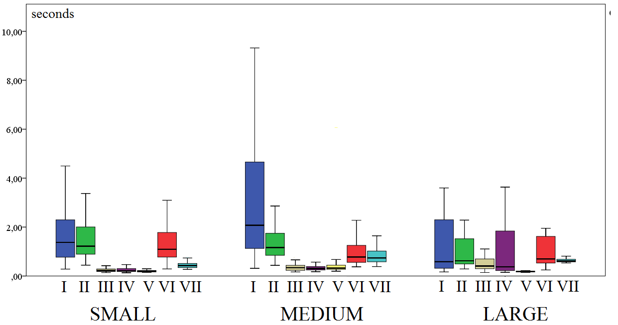
Figure 14: Time complexity of MIQP (the second step o ISC algorithm) for 3 test systems and 7 partitioning strategies. The median time and quartile boundaries are presented.

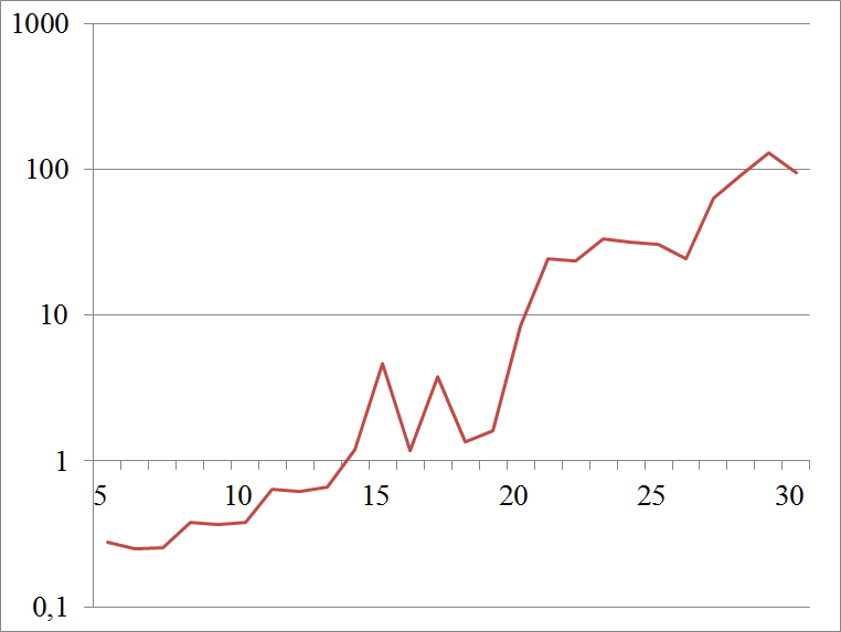
Figure 15: Time complexity of MIQP vs order of aggregated graph being partitioned (logarithmic scale).

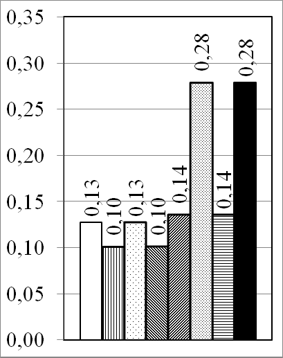
(a) SMALL system

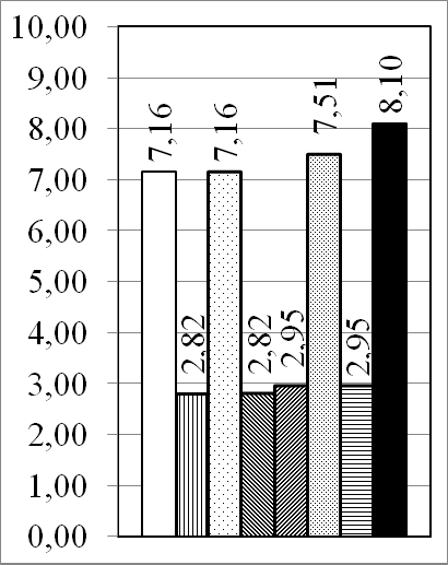
(b) MEDIUM system

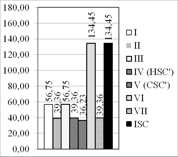
(c) LARGE system

Figure 16: Average time of eigenvectors’ calculation (the first step of ISC) for 7 parallel strategies of ISC algorithm. Eigenvectors were evaluated with eigs routine of Matlab R2014a run on Intel Core i-5 3337U CPU (1.8 GHz) laptop.

Figure 16 shows that evaluation of eigenvectors of the normalized Laplace matrix is the most computationally expensive operation of spectral clustering algorithms (at least, for realistically sized grids). Its complexity depends on the number of eigenvectors requested, on matrix dimension, and on its sparsity ratio.

In Strategies I and III $r_{1}K$ eigenvectors of matrix $L_{sym}(A|\mathbf{w})=L_{sym}(\alpha_{C}\Phi+\alpha_{D}|P|~{}|\mathbf{w})$ are calculated. Strategies II and IV require calculation of $r_{2}K$ eigenvectors of $L_{sym}(|P|~{}|\mathbf{w})$. The latter matrix is sparser and, therefore, the first step of Strategies I and III is computationally more expensive than that of Strategies II and IV.

Strategy V (CSC-based algorithm) is slightly more computationally expensive than Strategy IV (HSC-based) for SMALL and MEDIUM systems as it involves calculation of the eigenproblem for the Laplacian of denser matrix $\tilde{\Phi}$ of generators’ dynamic coupling. At the same time, for LARGE system Strategy V is faster than Strategy IV due to the smaller size of matrix $\tilde{\Phi}$.

Strategy VI involves the nested spectral bisection of $K$-partition and appears the most time-consuming strategy for all three test systems. On the other side, it is the most successful one (according to Table 3) and is very reliable in generating admissible (balanced) partitions. Comparing Figures 16 and 12 we see that Strategy II is approximately three times faster than Strategy IV and results in only minor loss of partitioning quality. Therefore, one may consider abandoning Strategy VI if it fails to satisfy application-specific time limits.

Strategy VII takes partitions $\pi_{\text{IV}}$ and $\pi_{\text{V}}$ as an input, so its computation time is the maximum of those for Strategies IV and V (computation time of the meet operation can be neglected).

For SMALL system eigenvector calculation is very fast, and, hence, ISC algorithm is slower than CSC quiros2015constrained and HSC sanchez2014AdmittanceDisruptionHierSpec algorithms (mostly, due to the additional second step, which takes about 2 sec. irrespective of the system dimension). For MEDIUM system the speed is comparable (15 seconds is reported for HSC sanchez2014AdmittanceDisruptionHierSpec , while CSC algorithm was tested only for the reduced Great Britain 815-bus system in sanchez2014AdmittanceDisruptionHierSpec ). These algorithms cannot be directly compared for LARGE system, since CSC and HSC fail to provide eligibly balanced partitions. If we relax the maximum island volume constraint, we can expect ISC to be at least three times slower than CSC and HSC, mostly due to the slow Strategy VI (which, as noted above, can be abandoned in case of time deficit).

It should be noted that for LARGE system (and, perhaps, for MEDIUM system) neither of existing spectral-clustering-based algorithms is fast enough for online islanding, when run on a PC. Eigenvectors’ calculation takes most time, and, fortunately, it can be dramatically fostered by using parallel vector calculus capabilities of graphical processing units (GPU) lessig2007eigenvalue ; bell2008efficient . Hence, fast implementation of eigenvector calculation for spectral clustering OCI algorithms in large power systems is no more than a programming issue. Potentially, the performance improvement can also be obtained by replacing spectral clustering with some algorithms of $NCut$ minimization based on semidefinite programming fan2012multi ; ames2014guaranteed . A yet another promising approach is to use deep learning techniques to replace the optimization problem solution with fast calculation by a multilayered artificial neural network. In this case the algorithm proposed in this article calculates an extensive data set used to learn the neural network. Comparison of these approaches requires additional work.

7 Conclusion

An improved version of spectral-clustering-based OCI algorithms sanchez2014AdmittanceDisruptionHierSpec ; quiros2015constrained is proposed in this article, which accounts for generator coherency, power flow disruption, shed load, and island size, allowing to adjust flexibly relative importance of these performance metrics and caring for the maximum island volume.

An optimal islanding scheme is sought in two steps. Firstly, several alternative detailed grid partitions are determined that contain more islands than required while balancing generator coherency and power flow disruption. Secondly, some islands in these partitions are merged to optimize the weighted sum of generator coherency, power flow disruption, and shed load while fulfilling the maximum island volume constraint. The second step reduces to MILP whose dimension does not depend on the dimension of the original grid and is small enough to use exact algorithms.

A series of experiments for three standard test grids was performed. The results show that, compared to competing algorithms, HSC sanchez2014AdmittanceDisruptionHierSpec and CSC quiros2015constrained , the proposed improved spectral clustering algorithm results in substantial improvement of both the overall composite criterion of partition quality (more than twice for some grids) and of each its component. The algorithm is computationally efficient. Potentially, it can be used to partition large power systems in real time.

The proposed algorithm can also be helpful in applications other than energy systems to partition high-dimensional directed graphs with asymmetric matrix of vertex weights.

The multi-objective criterion studied is a weighted sum of various performance metrics (generators’ dynamic coupling, power flow disruption, ECI, excess demand, shed load, and, probably, others), but the choice of performance metrics included into the optimization criterion and assignment of their relative weights is an open question in general. Further research is needed to establish an empirically grounded relation between transient stability of an island being created (e.g., with simulation techniques from ames2014guaranteed ; song2016dynamic ) and computationally efficient performance metrics (some of which were mentioned above).

- (1) CASE2383WP Power flow data for Polish system - winter 1999-2000 peak. http://www.pserc.cornell.edu/matpower/docs/ref/matpower5.0/case2383wp.html (2014). [Online; accessed July 08 2016]
- (2) Ahmed, S.S., Sarker, N.C., Khairuddin, A.B., Ghani, M.R.B.A., Ahmad, H.: A scheme for controlled islanding to prevent subsequent blackout. Power Systems, IEEE Transactions on 18(1), 136–143 (2003)
- (3) Ames, B.P.: Guaranteed clustering and biclustering via semidefinite programming. Mathematical Programming 147(1-2), 429–465 (2014)
- (4) Ariff, M., Pal, B.C.: Coherency identification in interconnected power system an independent component analysis approach. Power Systems, IEEE Transactions on 28(2), 1747–1755 (2013)
- (5) Bell, N., Garland, M.: Efficient sparse matrix-vector multiplication on cuda. Tech. rep., Nvidia Technical Report NVR-2008-004, Nvidia Corporation (2008)
- (6) Bie, T., Suykens, J., Moor, B.: Learning from general label constraints. In: Statistical Pattern Recognition, 2004. Proceedings of the 2004 IAPR International Workshop on, Lisbon, Portugal. IAPR (2004)
- (7) Butyrin, P., Vaskovskaya, T.: Diagnostika elektricheskikh tsepey po chastyam: Teoreticheskiye osnovy i komp’yuterniy praktikum. Moscow: MPEI Publishing House (2003)
- (8) Chow, J., Kokotovic, P.: Time scale modeling of dynamic networks with sparse and weak connections. In: Singular perturbations and asymptotic analysis in control systems, pp. 310–353. Springer (1987)
- (9) Chow, J.H., Galarza, R., Accari, P., Price, W.W.: Inertial and slow coherency aggregation algorithms for power system dynamic model reduction. Power Systems, IEEE Transactions on 10(2), 680–685 (1995)
- (10) Chow, J.H., et al.: A nodal aggregation algorithm for linearized two-time-scale power networks. In: Circuits and Systems, 1988., IEEE International Symposium on, pp. 669–672. IEEE (1988)
- (11) Chow, J.H., et al.: Aggregation properties of linearized two-time-scale power networks. Circuits and Systems, IEEE Transactions on 38(7), 720–730 (1991)
- (12) Christie, R.: 118 Bus Power Flow Test Case. https://www.ee.washington.edu/research/pstca/pf118/pg_tca118bus.htm (1993). [Online; accessed July 08 2016]
- (13) Cotilla-Sanchez, E., Hines, P.D., Barrows, C., Blumsack, S., Patel, M.: Multi-attribute partitioning of power networks based on electrical distance. Power Systems, IEEE Transactions on 28(4), 4979–4987 (2013)
- (14) Defays, D.: An efficient algorithm for a complete link method. The Computer Journal 20(4), 364–366 (1977)
- (15) Demetriou, P., Quirós-Tortós, J., Kyriakides, E., Terzija, V.: On implementing a spectral clustering controlled islanding algorithm in real power systems. In: PowerTech (POWERTECH), 2013 IEEE Grenoble, pp. 1–6. IEEE (2013)
- (16) Ding, L., Gonzalez-Longatt, F.M., Wall, P., Terzija, V.: Two-step spectral clustering controlled islanding algorithm. Power Systems, IEEE Transactions on 28(1), 75–84 (2013)
- (17) Ding, L., Wall, P., Terzija, V.: Constrained spectral clustering based controlled islanding. International Journal of Electrical Power & Energy Systems 63, 687–694 (2014)
- (18) Ding, T., Sun, K., Huang, C., Bie, Z., Li, F.: Mixed-integer linear programming-based splitting strategies for power system islanding operation considering network connectivity
- (19) El-Werfelli, M., Brooks, J., Dunn, R.: Controlled islanding scheme for power systems. In: Universities Power Engineering Conference, 2008. UPEC 2008. 43rd International, pp. 1–6. IEEE (2008)
- (20) Fan, N., Izraelevitz, D., Pan, F., Pardalos, P.M., Wang, J.: A mixed integer programming approach for optimal power grid intentional islanding. Energy Systems 3(1), 77–93 (2012)
- (21) Fan, N., Pardalos, P.M.: Multi-way clustering and biclustering by the ratio cut and normalized cut in graphs. Journal of combinatorial optimization 23(2), 224–251 (2012)
- (22) Fliscounakis, S., Panciatici, P., Capitanescu, F., Wehenkel, L.: Contingency ranking with respect to overloads in very large power systems taking into account uncertainty, preventive, and corrective actions. Power Systems, IEEE Transactions on 28(4), 4909–4917 (2013)
- (23) Garey, M., Johnson, D.: D. S, Johnson (1979) Computers and Intractability: A Guide to the Theory of NP-completeness. Freeman, San Francisco
- (24) Golari, M., Fan, N., Wang, J.: Two-stage stochastic optimal islanding operations under severe multiple contingencies in power grids. Electric Power Systems Research 114, 68–77 (2014)
- (25) Golari, M., Fan, N., Wang, J.: Large-scale stochastic power grid islanding operations by line switching and controlled load shedding. Energy Systems pp. 1–21 (2016). DOI 10.1007/s12667-016-0215-7
- (26) Goldschmidt, O., Hochbaum, D.S.: Polynomial algorithm for the k-cut problem (1988)
- (27) Hamon, C., Shayesteh, E., Amelin, M., Söder, L.: Two partitioning methods for multi-area studies in large power systems. International Transactions on Electrical Energy Systems 25(4), 648–660 (2015)
- (28) Juarez, C., Messina, A., Castellanos, R., Espinosa-Perez, G.: Characterization of multimachine system behavior using a hierarchical trajectory cluster analysis. Power Systems, IEEE Transactions on 26(3), 972–981 (2011)
- (29) Juncheng, S., Jiping, J., Famin, C., Lei, D.: Research on power system controlled islanding
- (30) Kundur, P., Paserba, J., Ajjarapu, V., Andersson, G., Bose, A., Canizares, C., Hatziargyriou, N., Hill, D., Stankovic, A., Taylor, C., et al.: Definition and classification of power system stability ieee/cigre joint task force on stability terms and definitions. Power Systems, IEEE Transactions on 19(3), 1387–1401 (2004)
- (31) Lessig, C.: Eigenvalue computation with cuda. NVIDIA techreport (2007)
- (32) Li, H., Rosenwald, G.W., Jung, J., Liu, C.C.: Strategic power infrastructure defense. Proceedings of the IEEE 93(5), 918–933 (2005)
- (33) Lütkepohl, H.: Handbook of matrices. John Wiley&Sons
- (34) Ng, A.Y., Jordan, M.I., Weiss, Y., et al.: On spectral clustering: Analysis and an algorithm. Advances in neural information processing systems 2, 849–856 (2002)
- (35) Pahwa, S., Youssef, M., Schumm, P., Scoglio, C., Schulz, N.: Optimal intentional islanding to enhance the robustness of power grid networks. Physica A: Statistical Mechanics and its Applications 392(17), 3741–3754 (2013)
- (36) Peiravi, A., Ildarabadi, R.: A fast algorithm for intentional islanding of power systems using the multilevel kernel k-means approach. Journal of Applied Sciences 9(12), 2247–2255 (2009)
- (37) Quirós-Tortós, J., Sánchez-García, R., Brodzki, J., Bialek, J., Terzija, V.: Constrained spectral clustering-based methodology for intentional controlled islanding of large-scale power systems. Generation, Transmission & Distribution, IET 9(1), 31–42 (2015)
- (38) Quirós-Tortós, J., Wall, P., Ding, L., Terzija, V.: Determination of sectionalising strategies for parallel power system restoration: A spectral clustering-based methodology. Electric Power Systems Research 116, 381–390 (2014)
- (39) Sánchez-García, R.J., Fennelly, M., Norris, S., Wright, N., Niblo, G., Brodzki, J., Bialek, J.W.: Hierarchical spectral clustering of power grids. Power Systems, IEEE Transactions on 29(5), 2229–2237 (2014)
- (40) Song, J., Cotilla-Sanchez, E., Ghanavati, G., Hines, P.D.H.: Dynamic modeling of cascading failure in power systems. Power Systems, IEEE Transactions on pp. 2085 –2095 (2016)
- (41) Sun, K., Zheng, D.Z., Lu, Q.: Splitting strategies for islanding operation of large-scale power systems using obdd-based methods. Power Systems, IEEE Transactions on 18(2), 912–923 (2003)
- (42) Trodden, P., Bukhsh, W., Grothey, A., McKinnon, K.: Milp formulation for controlled islanding of power networks. International Journal of Electrical Power & Energy Systems 45(1), 501–508 (2013)
- (43) Trodden, P.A., Bukhsh, W.A., Grothey, A., McKinnon, K.I.: Optimization-based islanding of power networks using piecewise linear ac power flow. Power Systems, IEEE Transactions on 29(3), 1212–1220 (2014)
- (44) Vittal, V., Kliemann, W., Ni, Y., Chapman, D., Silk, A., Sobajic, D.: Determination of generator groupings for an islanding scheme in the manitoba hydro system using the method of normal forms. Power Systems, IEEE Transactions on 13(4), 1345–1351 (1998)
- (45) Von Luxburg, U.: A tutorial on spectral clustering. Statistics and computing 17(4), 395–416 (2007)
- (46) Wang, X., Vittal, V.: System islanding using minimal cutsets with minimum net flow. In: Power Systems Conference and Exposition, 2004. IEEE PES, pp. 379–384. IEEE (2004)
- (47) Ward Jr, J.H.: Hierarchical grouping to optimize an objective function. Journal of the American statistical association 58(301), 236–244 (1963)
- (48) Xu, G., Vittal, V.: Slow coherency based cutset determination algorithm for large power systems. Power Systems, IEEE Transactions on 25(2), 877–884 (2010)
- (49) Yang, B., Vittal, V., Heydt, G.T., Sen, A.: A novel slow coherency based graph theoretic islanding strategy. In: Power Engineering Society General Meeting, 2007. IEEE, pp. 1–7. IEEE (2007)
- (50) You, H., Vittal, V., Wang, X.: Slow coherency-based islanding. Power Systems, IEEE Transactions on 19(1), 483–491 (2004)
- (51) Yusof, S., Rogers, G., Alden, R.: Slow coherency based network partitioning including load buses. Power Systems, IEEE Transactions on 8(3), 1375–1382 (1993)
- (52) Zhao, Q., Sun, K., Zheng, D.Z., Ma, J., Lu, Q.: A study of system splitting strategies for island operation of power system: A two-phase method based on obdds. Power Systems, IEEE Transactions on 18(4), 1556–1565 (2003)
- (53) Zimmerman, R.D., Murillo-Sánchez, C.E., Thomas, R.J.: Matpower: Steady-state operations, planning, and analysis tools for power systems research and education. Power Systems, IEEE Transactions on 26(1), 12–19 (2011)