Nutational resonances, transitional precession, and precession-averaged evolution in binary black-hole systems

Abstract

In the post-Newtonian (PN) regime, the timescale on which the spins of binary black holes precess is much shorter than the radiation-reaction timescale on which the black holes inspiral to smaller separations. On the precession timescale, the angle between the total and orbital angular momenta oscillates with nutation period $\tau$, during which the orbital angular momentum precesses about the total angular momentum by an angle $\alpha$. This defines two distinct frequencies that vary on the radiation-reaction timescale: the nutation frequency $\omega\equiv 2\pi/\tau$ and the precession frequency $\Omega\equiv\alpha/\tau$. We use analytic solutions for generic spin precession at 2PN order to derive Fourier series for the total and orbital angular momenta in which each term is a sinusoid with frequency $\Omega-n\omega$ for integer $n$. As black holes inspiral, they can pass through nutational resonances ($\Omega=n\omega$) at which the total angular momentum tilts. We derive an approximate expression for this tilt angle and show that it is usually less than $10^{-3}$ radians for nutational resonances at binary separations $r>10M$. The large tilts occurring during transitional precession (near zero total angular momentum) are a consequence of such states being approximate $n=0$ nutational resonances. Our new Fourier series for the total and orbital angular momenta converge rapidly with $n$ providing an intuitive and computationally efficient approach to understanding generic precession that may facilitate future calculations of gravitational waveforms in the PN regime.

I Introduction

The discovery of gravitational waves (GWs) emitted by binary black holes (BBHs) Abbott et al. (2016a, b, c) provides powerful motivation to better understand the generic behavior of such systems. BBH mergers can be divided into three stages: the inspiral during which the BBHs approach each other as their orbit decays due to radiation reaction, the merger proper in which the two BBH event horizons coalesce into the single horizon of the final black hole, and the ringdown in which the final black hole settles down to an unperturbed Kerr solution describing an isolated spinning black hole Kerr (1963). The evolution during each of these three stages is best described by a different numerical technique. The post-Newtonian (PN) approximation pioneered by Einstein himself Einstein (1915) works well during the inspiral stage when the binary separation $r$ is much greater than than the gravitational radius $r_{g}\equiv GM/c^{2}$, where $M=m_{1}+m_{2}$ is the sum of the BBH masses $m_{i}$, $G$ is Newton’s gravitational constant, and $c$ is the speed of light. Numerical relativity Pretorius (2005); Campanelli et al. (2006); Baker et al. (2006) is required to describe the final orbits and merger proper, while black-hole perturbation theory Regge and Wheeler (1957); Zerilli (1970); Teukolsky (1973) provides a good description of the late ringdown when the spacetime is close to the Kerr solution describing the final black hole.

This paper will focus on the inspiral stage of the merger at binary separations $r\gg r_{g}$ for which the PN approximation is valid. This stage is important for several reasons. BBHs with $M\lesssim 25M_{\odot}$ [such as the system responsible for GW151226 Abbott et al. (2016b), the second detection by the Laser Interferometer Gravitational-wave Observatory (LIGO)] are well described by a PN inspiral when emitting GWs at the lower end of the LIGO sensitivity band. Although the PN regime does not fall within the LIGO band for more massive systems like the one responsible for the first LIGO detection GW150914 Abbott et al. (2016a), in the future such systems may be detectable in the PN regime at lower GW frequencies by space-based observatories such as LISA Sesana (2016). Finally, the PN approximation is essential for evolving BBHs from the wide separations at which they form to the smaller separations at which they emit detectable GWs Kesden et al. (2015); Gerosa et al. (2015a); Gerosa and Kesden (2016). This evolution is required for efforts to use BBH spins to distinguish between different astrophysical models of BBH formation Kesden et al. (2010a, b); Berti et al. (2012); Gerosa et al. (2013); Rodriguez et al. (2016); Stevenson et al. (2017).

In the PN regime, BBHs evolve on three distinct timescales:

$$t_{\rm orb} \equiv\left(\frac{r^{3}}{GM}\right)^{1/2},$$ (1a)

$$t_{\rm pre} \equiv\frac{c^{2}r^{5/2}}{(GM)^{3/2}}=\left(\frac{r}{r_{g}}\right)t_{\rm orb},$$ (1b)

$$t_{\rm RR} \equiv\frac{c^{5}r^{4}}{(GM)^{3}}=\left(\frac{r}{r_{g}}\right)^{5/2}t_{\rm orb},$$ (1c)

where the direction of the binary separation vector $\mathbf{r}$ changes on the orbital timescale $t_{\rm orb}$, the directions of the BBH spins $\mathbf{S}_{i}$ and orbital angular momentum $\mathbf{L}$ change on the precession timescale $t_{\rm pre}$, and the binary separation $r$ shrinks on the radiation-reaction timescale $t_{\rm RR}$. The validity of the PN approximation ($r\gg r_{g}$) implies that these timescales obey the hierarchy $t_{\rm orb}\ll t_{\rm pre}\ll t_{\rm RR}$. This hierarchy suggests that BBH dynamics can be understood through a multi-timescale analysis: the evolution on a given timescale can be solved by holding constant quantities evolving on longer timescales and time-averaging quantities evolving on shorter timescales.

In the case of BBH evolution, a multi-timescale analysis requires two different kinds of averaging: using Keplerian or higher PN-order solutions to the two-body problem to orbit average when considering evolution on the precession or radiation-reaction timescales, and using PN solutions to the spin-precession equations to precession average when considering evolution on the radiation-reaction timescale. Orbit averaging using either circular or eccentric Keplerian orbits has been employed in many previous studies of solutions to the spin-precession equations Apostolatos et al. (1994); Kidder (1995); Schnittman (2004). In previous work Kesden et al. (2015); Gerosa et al. (2015a), we derived analytic solutions to the 2PN spin-precession equations, allowing us to precession average BBH dynamics at this PN order for the first time. This precession averaging has led to a vast increase in computational efficiency when evolving BBH spins on the radiation-reaction timescale as binaries inspiral from wide separations into the LIGO band. Readers can take advantage of these computational savings by using the publicly available python module precession Gerosa and Kesden (2016).

In this paper, we make further use of precession averaging to derive a new series expansion for the generic evolution of the orbital angular momentum $\mathbf{L}$ on the precession timescale. This expansion is highly analogous to a Fourier series, with amplitudes and frequencies varying on the longer radiation-reaction timescale. This analysis is complicated by the fact that precession exhibits two distinct frequencies. The nutation frequency $\omega\equiv 2\pi/\tau$ is the frequency with which the angle $\theta_{L}$ between $\mathbf{L}$ and the total angular momentum $\mathbf{J}$ oscillates, where $\tau$ is the period of these oscillations. The precession frequency $\Omega\equiv\alpha/\tau$ is the average rate at which $\mathbf{L}$ precesses in a cone about $\mathbf{J}$, where $\alpha$ is the precession angle over the nutation period $\tau$. Each term in our series expansion corresponds to simple precession of a vector in the plane perpendicular to the precession-averaged $\langle\mathbf{J}\rangle$, with the magnitude of each vector fixed on the precession timescale and the precession frequency given by $\Omega-n\omega$ for integer $n$. The magnitude of the component of $\mathbf{L}$ parallel to $\langle\mathbf{J}\rangle$ is chosen to maintain the proper normalization of $\mathbf{L}$. This expansion converges rapidly with $n$, implying that it may be useful in the construction of frequency-domain waveforms for the inspiral portion of BBH mergers. Our analytic solutions to the spin-precession equations have already been used for waveform construction in recent work Chatziioannou et al. (2017a, b). We hope that the new precession-averaged expansions for $\mathbf{L}$ and $\mathbf{J}$ developed later in this paper will be similarly useful, as variation in the direction of $\mathbf{J}$ is a major source of error for these efforts.

Our new series expansion has also revealed the existence of nutational resonances where $\Omega=n\omega$. At such resonances, the precession-averaged rate $\langle d\mathbf{J}/dt\rangle$ at which the total angular momentum is radiated is misaligned with $\langle\mathbf{J}\rangle$, implying that $\langle\mathbf{J}\rangle$ is tilting on the precession timescale. Although the resonance condition $\Omega=n\omega$ is finely tuned at any given binary separation $r$, generic BBHs often cross resonances as they inspiral from wide separations towards merger. We derive approximate expressions for the angle $\theta_{\rm tilt}$ through which $\langle\mathbf{J}\rangle$ tilts at a resonance and show that such tilts are usually below $10^{-3}$ radians making them negligible for the purpose of GW data analysis. An exception is the large tilts that occur during transition precession Apostolatos et al. (1994), which can be interpreted as an approximate $n=0$ nutational resonance in much of the parameter space with near-vanishing total angular momentum ($J\simeq 0$).

The remainder of this paper is organized as follows. Section II reviews our previous work Kesden et al. (2015); Gerosa et al. (2015a) on analytic solutions to the orbit-averaged spin-precession equations. In Section III, we make use of these solutions to derive a new series expansion for the evolution of the orbital angular momentum $\mathbf{L}$ on the precession timescale. We show that only a few terms in this expansion with the lowest values of $|n|$ are required to produce excellent agreement with full numerical solutions of the orbit-averaged spin-precession equations, and explore the implications of this expansion for the evolution of the total angular momentum $\mathbf{J}$. In Section IV, we show that $\langle\mathbf{J}\rangle$ tilts at nutational resonances where $\Omega=n\omega$ and derive an approximate expression for the tilt angle $\theta_{\rm tilt}$ that we verify agrees well with the tilts observed in full numerical solutions of the orbit-averaged spin-precession equations. In Section V, we examine how often generic binaries encounter nutational resonances during their inspirals and the distribution of tilt angles at these resonances. In Sec. VI, we explore the connection between our newly discovered nutational resonances and transitional precession near $J\simeq 0$ Apostolatos et al. (1994). Some concluding remarks are provided in Section VII. In the rest of this paper, we will use relativists’ units where $G=c=1$.

II Review of Spin Precession

Consider binary black holes on a quasicircular orbit with masses $m_{1}$ and $m_{2}$, mass ratio $q\equiv m_{2}/m_{1}\leq 1$, total mass $M\equiv m_{1}+m_{2}$, and symmetric mass ratio $\eta\equiv m_{1}m_{2}/M^{2}=q/(1+q)^{2}$. Such a system will have an orbital angular momentum $\mathbf{L}$ with magnitude $L=\eta(M^{3}r)^{1/2}$ to lowest PN order and spins $\mathbf{S}_{i}$ with magnitudes $S_{i}=\chi_{i}m_{i}^{2}$, where the dimensionless spins have magnitudes $0\leq\chi_{i}\leq 1$. The total spin $\mathbf{S}=\mathbf{S}_{1}+\mathbf{S}_{2}$ has magnitude $S$, and the total angular momentum $\mathbf{J}=\mathbf{L}+\mathbf{S}$ has magnitude $J$. Each of these quantities is either constant or evolves on one of the timescales given by Eq. (1). At the PN order we consider in this paper, the masses $m_{i}$ and dimensionless spin magnitudes $\chi_{i}$ are constant throughout the inspiral. The projected effective spin

$$\xi\equiv\frac{1}{M^{2}}\left[\left(1+q\right)\mathbf{S}_{1}+\left(1+\frac{1}{q}\right)\mathbf{S}_{2}\right]\cdot\hat{\mathbf{L}}~{},$$ (2)

referred to as $\chi_{\rm eff}$ in LIGO parameter estimation, is constant on the precession timescale $t_{\rm pre}$ Damour (2001); Racine (2008) and is also constant throughout the inspiral to the PN order we consider. The magnitudes $L$ and $J$ of the orbital and total angular momenta evolve on the radiation-reaction timescale $t_{\rm RR}$. It is sometimes convenient to define an additional quantity

$$\kappa\equiv\frac{J^{2}-L^{2}}{2L}=\mathbf{S}\cdot\mathbf{\hat{L}}+\frac{S^{2}}{2L}~{},$$ (3)

because the limit

$$\lim_{r\to\infty}\kappa\equiv\kappa_{\infty}=S_{1}\cos\theta_{1\infty}+S_{2}\cos\theta_{2\infty}$$ (4)

is a finite constant that can be used to label BBHs throughout their inspiral. In this expression, $\theta_{i\infty}$ is the angle between $\mathbf{S}_{i}$ and $\mathbf{L}$ in the limit $r\to\infty$; this angle is a constant since in this limit spin-orbit coupling dominates over spin-spin coupling and the two spins $\mathbf{S}_{i}$ simply precess about the orbital angular momentum $\mathbf{L}$. The total spin $\mathbf{S}$, as well as the directions of $\mathbf{S}_{i}$, $\mathbf{L}$, and $\mathbf{J}$ all evolve on the precession timescale $t_{\rm pre}$.

This last point is somewhat subtle, since in the absence of gravitational radiation, the magnitude and direction of the total angular momentum $\mathbf{J}$ are both conserved. In the case of simple precession, $\mathbf{L}$ and $\mathbf{J}$ precess on cones with opening angles $\theta_{Lz}$ and $\theta_{J}$ respectively about a fixed direction $\mathbf{\hat{z}}$ in an inertial frame Apostolatos et al. (1994). The timescale hierarchy $t_{\rm pre}/t_{\rm RR}=(r/r_{g})^{-3/2}\ll 1$ implies that $\theta_{J}/\theta_{Lz}\propto(r/r_{g})^{-3/2}\ll 1$, but the frequency $\Omega$ with which $\mathbf{L}$ and $\mathbf{J}$ precess about their cones is the same and of order the inverse of the precession timescale $t_{\rm pre}$. Although generic spin precession is more complicated, the direction of the total angular momentum $\mathbf{J}$ still evolves (by a small angle) on the precession timescale.

In previous work Kesden et al. (2015); Gerosa et al. (2015a), we analyzed generic spin precession under the approximation, valid in the absence of radiation reaction, that the direction of $\mathbf{J}$ stays fixed. In this section, we summarize key results from that work which we will use in the following section where we relax the assumption that the direction of $\mathbf{J}$ stays fixed. The many constants of motion on the precession timescale listed above imply that there is only a single degree of freedom in the relative orientations of $\mathbf{L}$, $\mathbf{S}_{1}$, and $\mathbf{S}_{2}$, which we can conveniently specify by choosing the magnitude $S$ of the total spin as a general coordinate. For precisely equal masses ($q=1$), $S$ is constant and an alternative coordinate is required to specify this degree of freedom Gerosa et al. (2017). The angle $\theta_{L}$ between $\mathbf{L}$ and $\mathbf{J}$ is given in terms of $S$ by the expression

$$\cos\theta_{L}=\frac{J^{2}+L^{2}-S^{2}}{2JL}~{}.$$ (5)

The hierarchy $\theta_{J}\ll\theta_{Lz}$ in the PN regime implies that $\theta_{Lz}\simeq\theta_{L}$ to high accuracy. The relative orientation of $\mathbf{S}$, $\mathbf{L}$, and $\mathbf{J}$ in terms of this angle are shown in Fig. 1. The total spin magnitude $S$ oscillates in the range $S_{-}\leq S\leq S_{+}$, where the extrema $S_{\pm}$ are the roots of the equation $\xi=\xi_{\pm}(S)$, $\xi$ is the projected effective spin given by Eq. (2), and the two curves

$$\xi_{\pm}(S) =\{(J^{2}-L^{2}-S^{2})[S^{2}(1+q)^{2}-(S_{1}^{2}-S_{2}^{2})(1-q^{2})]$$

$$\quad\pm(1-q^{2})A_{1}A_{2}A_{3}A_{4}\}/(4qM^{2}S^{2}L)$$ (6)

form a closed loop we called the effective potential for spin precession. In this expression, we have used four auxiliary functions $A_{i}$ which are defined as

$$A_{1} \equiv[J^{2}-(L-S)^{2}]^{1/2}\,,$$ (7a)

$$A_{2} \equiv[(L+S)^{2}-J^{2}]^{1/2}\,,$$ (7b)

$$A_{3} \equiv[S^{2}-(S_{1}-S_{2})^{2}]^{1/2}\,,$$ (7c)

$$A_{4} \equiv[(S_{1}+S_{2})^{2}-S^{2}]^{1/2}\,.$$ (7d)

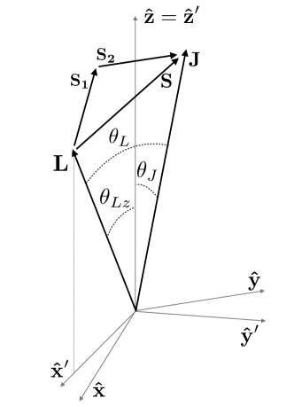
Figure 1: References frames useful for describing BBH spin precession. The total spin $\mathbf{S}$ is the sum of the spins $\mathbf{S}_{1}$ and $\mathbf{S}_{2}$ of the more massive and less massive black holes. The total angular momentum $\mathbf{J}$ is the sum of the orbital angular momentum $\mathbf{L}$ and total spin $\mathbf{S}$, and $\theta_{L}$ is the angle between $\mathbf{L}$ and $\mathbf{J}$. We define the $xyz$ inertial frame such that $\mathbf{\hat{z}}$ points in the direction of the precession-averaged orbital and total angular momenta $\langle\mathbf{L}\rangle$ and $\langle\mathbf{J}\rangle$ after many precession cycles. The basis vectors $\mathbf{\hat{x}}$ and $\mathbf{\hat{y}}$ complete the orthonormal triad. The angles between $\mathbf{\hat{z}}$ and $\mathbf{L}$ and $\mathbf{J}$ are given by $\theta_{Lz}$ and $\theta_{J}$ respectively; the hierarchy $\theta_{J}\ll\theta_{Lz}$ implies that $\theta_{Lz}\simeq\theta_{L}$. After a nutation period $\tau$, $\mathbf{L}$ and $\mathbf{J}$ precess about $\mathbf{\hat{z}}$ by an angle $\alpha$. We use these quantities to define the $x^{\prime}y^{\prime}z^{\prime}$ rotating frame in which $\mathbf{\hat{z}^{\prime}}=\mathbf{\hat{z}}$ and $\mathbf{\hat{x}^{\prime}}$ and $\mathbf{\hat{y}^{\prime}}$ precess about $\mathbf{\hat{z}}$ with precession frequency $\Omega=\alpha/\tau$.

Fig. 1 shows that the oscillations of $S$ correspond to nutation of the orbital angular momentum $\mathbf{L}$, allowing us to define the nutation period

$$\tau=2\int_{S_{-}}^{S_{+}}\frac{dS}{|dS/dt|}~{}.$$ (8)

and nutation frequency $\omega\equiv 2\pi/\tau$. Note that in our earlier work Kesden et al. (2015); Gerosa et al. (2015a); Gerosa and Kesden (2016), we referred to $\tau$ as the precession period because we were focused on the relative orientations of the BBH spins and it has the precession timescale. The nutation frequency only depends on quantities varying on the radiation-reaction timescale. The time derivative of the total spin magnitude $S$ is

$$\frac{dS}{dt}= -\frac{3(1-q^{2})}{2q}\frac{S_{1}S_{2}}{S}\frac{(\eta^{2}M^{3})^{3}}{L^{5}}\left(1-\frac{\eta M^{2}\xi}{L}\right)$$

$$\times\sin\theta_{1}\sin\theta_{2}\sin\Delta\Phi~{},$$ (9)

where the angles $\theta_{i}$ between $\mathbf{L}$ and $\mathbf{S}_{i}$ are given by

$$\cos\theta_{1} =\frac{1}{2(1-q)S_{1}}\left[\frac{J^{2}-L^{2}-S^{2}}{L}-\frac{2qM^{2}\xi}{1+q}\right]\,,$$ (10a)

$$\cos\theta_{2} =\frac{q}{2(1-q)S_{2}}\left[-\frac{J^{2}-L^{2}-S^{2}}{L}+\frac{2M^{2}\xi}{1+q}\right]\,.$$ (10b)

The angle $\Delta\Phi$ between the projections of $\mathbf{S}_{1}$ and $\mathbf{S}_{2}$ orthogonal to $\mathbf{L}$ is given by

$$\cos\Delta\Phi=\frac{\cos\theta_{12}-\cos\theta_{1}\cos\theta_{2}}{\sin\theta_{1}\sin\theta_{2}}\,,$$ (11)

where

$$\cos\theta_{12}=\frac{S^{2}-S_{1}^{2}-S_{2}^{2}}{2S_{1}S_{2}}$$ (12)

is the cosine of the angle between $\mathbf{S}_{1}$ and $\mathbf{S}_{2}$.

Although $\mathbf{L}$, $\mathbf{S}_{1}$, and $\mathbf{S}_{2}$ return to their initial relative orientation after a nutation period $\tau$, in an inertial frame these vectors precess about $\mathbf{\hat{z}}$ by an angle

$$\alpha=2\int_{S_{-}}^{S_{+}}\Omega_{z}\frac{dS}{|dS/dt|}~{},$$ (13)

where

$$\Omega_{z} =\frac{J}{2}\left(\frac{\eta^{2}M^{3}}{L^{2}}\right)^{3}\bigg{\{}1+\frac{3}{2\eta}\left(1-\frac{\eta M^{2}\xi}{L}\right)$$

$$-\frac{3(1+q)}{2qA_{1}^{2}A_{2}^{2}}\left(1-\frac{\eta M^{2}\xi}{L}\right)[4(1-q)L^{2}(S_{1}^{2}-S_{2}^{2})$$

$$-(1+q)(J^{2}-L^{2}-S^{2})(J^{2}-L^{2}-S^{2}-4\eta M^{2}L\xi)]\bigg{\}}$$ (14)

is the instantaneous precession frequency. Note that in our earlier work, we identified $\mathbf{\hat{z}}$ with the instantaneous direction of the total angular momentum $\mathbf{J}$ rather than its precession average $\langle\mathbf{J}\rangle$, because we were neglecting the small changes to the direction of $\mathbf{J}$ compared to that of $\mathbf{L}$ ($\theta_{J}\ll\theta_{L}$). These results allow us to define the average precession frequency $\Omega\equiv\alpha/\tau$. Although the nutation frequency $\omega$ and precession frequency $\Omega$ are both of order the inverse precession timescale $t_{\rm pre}$, they generally differ because $\alpha\neq 2\pi$. As shown in Fig. 1, we can define an orthonormal basis for our inertial frame by choosing vectors $\mathbf{\hat{x}}$ and $\mathbf{\hat{y}}$ perpendicular to $\mathbf{\hat{z}}$. We can also define a frame rotating about $\mathbf{\hat{z}}=\mathbf{\hat{z}}^{\prime}$ with precession frequency $\Omega$ with rotating basis vectors

$$\mathbf{\hat{x}}^{\prime} =\mathbf{\hat{x}}\cos\Omega t+\mathbf{\hat{y}}\sin\Omega t~{},$$ (15a)

$$\mathbf{\hat{y}}^{\prime} =-\mathbf{\hat{x}}\sin\Omega t+\mathbf{\hat{y}}\cos\Omega t~{}.$$ (15b)

In the quadrupole approximation, GW emission removes angular momentum from the binary at a rate Peters and Mathews (1963)

$$\frac{d\mathbf{J}}{dt}=-\frac{32}{5}\left(\frac{r}{M}\right)^{-4}\frac{\eta\mathbf{L}}{M}~{}.$$ (16)

The 1PN correction to this expression is also parallel to the orbital angular momentum $\mathbf{L}$ Kidder (1995). This expression implies that the magnitudes of $\mathbf{L}$ and $\mathbf{J}$ evolve according to the equations

$$\frac{dL}{dt} =\frac{d\mathbf{J}}{dt}\cdot\mathbf{\hat{L}}=-\frac{32}{5}\left(\frac{r}{M}\right)^{-4}\frac{\eta L}{M}~{},$$ (17a)

$$\frac{dJ}{dt} =\frac{d\mathbf{J}}{dt}\cdot\mathbf{\hat{J}}=\frac{dL}{dt}\cos\theta_{L}~{}.$$ (17b)

This expression for $dL/dt$ evolves on the radiation-reaction timescale, but the expression for $dJ/dt$ evolves on the precession timescale because of the angular term $\cos\theta_{L}$ given by Eq. (5). We can precession average the right-hand side of Eq. (17b) using

$$\langle\cos\theta_{L}\rangle=\frac{2}{\tau}\int_{S_{-}}^{S_{+}}\frac{\cos\theta_{L}~{}dS}{|dS/dt|}$$ (18)

to obtain the precession-averaged loss of total angular momentum $\langle dJ/dt\rangle=(dL/dt)\langle\cos\theta_{L}\rangle$ Kesden et al. (2015); Gerosa et al. (2015a). This equation and Eq. (17a) can be numerically integrated with a time step on the radiation-reaction timescale, providing a vast savings in computational time compared to a time step on the precession timescale if one is only interested in the relative orientations of $\mathbf{L}$, $\mathbf{S}_{1}$, and $\mathbf{S}_{2}$ specified by Eqs. (10) and (11) Gerosa et al. (2015a); Gerosa and Kesden (2016). However, to determine the directions of the vectors $\mathbf{L}$ and $\mathbf{J}$ in an inertial frame (perhaps for the purpose of calculating the emission of GWs), one must integrate the instantaneous precession frequency $\Omega_{z}$ given by Eq. (II) with a time step on the precession timescale. In the next section, we derive new series expansions for $\mathbf{L}$ and $\mathbf{J}$ in terms of quantities that only evolve on the radiation-reaction timescale which can in principle achieve similar computational savings to our earlier expression for $\langle dJ/dt\rangle$.

III A New Expansion

In the inertial (unprimed) frame defined in the previous section, we can decompose the orbital angular momentum

$$\mathbf{L}=L_{\parallel}\mathbf{\hat{z}}+\mathbf{L}_{\perp}$$ (19)

into components parallel and perpendicular to the direction $\mathbf{\hat{z}}$ of its precession average $\langle\mathbf{L}\rangle$. Without loss of generality, we can choose $\mathbf{L}$ to lie in the $xz$ plane at $t=0$ with total spin magnitude $S=S_{-}$. With this choice, the perpendicular component of $\mathbf{L}$ is given by

$$\mathbf{L}_{\perp}=L\sin\theta_{L}(\cos\Phi_{L}\mathbf{\hat{x}}+\sin\Phi_{L}\mathbf{\hat{y}})~{}.$$ (20)

The total spin magnitude $S(t)$ is an even function of time with period $\tau$, implying that it is fully specified by its values in the interval $0\leq t\leq\tau/2$. On this interval, $S(t)$ is the inverse of the function

$$t(S)=\int_{S_{-}}^{S}\frac{dS^{\prime}}{|dS/dt|}~{},$$ (21)

where $dS/dt$ is given by Eq. (II) and $S_{-}\leq S\leq S_{+}$. Eq. (5) indicates that $\theta_{L}$ is similarly a periodic, even function of time, while Eq. (II) requires $\Phi_{L}(t)$ to be a periodic, odd function of time defined by its values

$$\Phi_{L}(t)=\int_{0}^{t}\Omega_{z}~{}dt^{\prime}=\int_{S_{-}}^{S}\Omega_{z}\frac{dS^{\prime}}{|dS/dt|}$$ (22)

in the interval $0\leq t\leq\tau/2$. The symmetry and periodicity of $\theta_{L}$ and $\Phi_{L}$ imply that we can Fourier expand the perpendicular component of $\mathbf{L}$ in the rotating frame given by Eq. (15) to obtain the series

$$\mathbf{L}_{\perp}(t)=L\sum_{n=0}^{+\infty}[\theta_{Lxn}^{\prime}\cos(n\omega t)~{}\mathbf{\hat{x}}^{\prime}+\theta_{Lyn}^{\prime}\sin(n\omega t)~{}\mathbf{\hat{y}}^{\prime}]~{}.$$ (23)

Comparing Eqs. (20) and (23) and using Eq. (15) to relate the rotating and inertial frames, we see that

$$\theta_{Lxn}^{\prime} =\frac{2-\delta_{n0}}{L\tau}\int_{0}^{\tau}\mathbf{L}_{\perp}\cdot\mathbf{\hat{x}}^{\prime}\cos(n\omega t)~{}dt$$

$$=\frac{2}{\tau}\int_{S_{-}}^{S_{+}}\cos(\Phi_{L}-\Omega t)\sin\theta_{L}\cos(n\omega t)\frac{dS}{|dS/dt|}$$ (24)

and

$$\theta_{Lyn}^{\prime} =\frac{2-\delta_{n0}}{L\tau}\int_{0}^{\tau}\mathbf{L}_{\perp}\cdot\mathbf{\hat{y}}^{\prime}\sin(n\omega t)~{}dt$$

$$=\frac{4}{\tau}\int_{S_{-}}^{S_{+}}\sin(\Phi_{L}-\Omega t)\sin\theta_{L}\sin(n\omega t)\frac{dS}{|dS/dt|}~{},$$ (25)

where the Kronecker delta $\delta_{ij}$ equals unity for $i=j$ and zero otherwise. We can use Eqs. (15) and (23) to obtain an equivalent series for $\mathbf{L}_{\perp}$ in the inertial frame,

$$\mathbf{L}_{\perp}(t)=L\sum_{n=-\infty}^{+\infty}\theta_{Ln}\{\cos[(\Omega-n\omega)t]\mathbf{\hat{x}}+\sin[(\Omega-n\omega)t]\mathbf{\hat{y}}\}~{},$$ (26)

where

$$\theta_{Ln} =\frac{1+\delta_{n0}}{2}[\theta_{Lx|n|}^{\prime}-{\rm sgn}(n)\theta_{Ly|n|}^{\prime}]$$

$$=\frac{2}{\tau}\int_{S_{-}}^{S_{+}}\cos(\Phi_{L}-\Omega t+n\omega t)\sin\theta_{L}\frac{dS}{|dS/dt|}~{}.$$ (27)

One can obtain $\mathbf{L}$ from Eqs. (19) and (26) by recognizing that the magnitude of $\mathbf{L}$ is conserved on the precession timescale implying that

$$L_{\parallel}=\sqrt{L^{2}-\mathbf{L}_{\perp}\cdot\mathbf{L}_{\perp}}~{}.$$ (28)

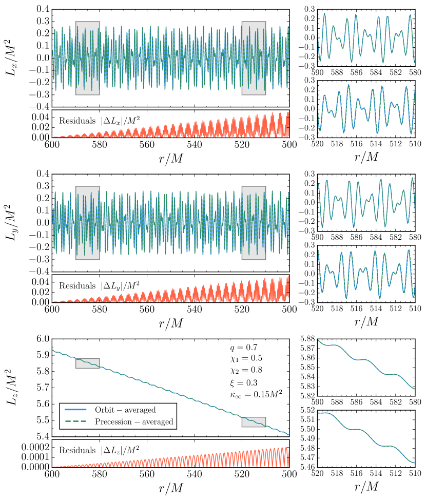
Figure 2: Comparison of the orbital angular momentum $L(t)$ determined from a numerical integration of the orbit-averaged spin-precession equations and our new precession-averaged series expansion given by Eq. (26). The binary has mass ratio $q=0.7$, dimensionless spin magnitudes $\chi_{1}=0.5$ and $\chi_{2}=0.8$, projected effective spin $\xi=0.3$, and asymptotic projected total spin $\kappa_{\infty}=0.15M^{2}$. It inspirals from binary separation $r=600M$ to $r=500M$. The top, middle, and bottom panels show the components of $\mathbf{L}$ in an inertial frame in which $\mathbf{\hat{z}}$ points in the direction of $\langle\mathbf{L}\rangle$, the precession-averaged orbital angular momentum. The solid blue curves show the orbit-averaged solution, the dashed green curves show our new precession-averaged solution, and the red curves below each panel show the magnitude of the differences between the solutions. We have only used the five terms corresponding to $n=0,\pm 1,\pm 2$ in the series expansion. The right panels show zoomed-in views of the inspiral from $r=590M$ to $r=580M$ and $r=520M$ to $r=510M$.

Eq. (26) is an elegant expression for $\mathbf{L}_{\perp}$; each term corresponds to a vector with magnitude $L|\theta_{Ln}|$ tracing out a circle with frequency $\Omega-n\omega$ in the plane orthogonal to $\mathbf{\hat{z}}$, the direction of the precession-averaged orbital angular momentum $\langle\mathbf{L}\rangle$. These magnitudes and frequencies are both evolving on the radiation-reaction timescale $t_{\rm RR}$, implying that they can be numerically evaluated throughout the inspiral with a time step of order $t_{\rm RR}$ leading to potentially large computational savings. Eq. (26) also seems well suited for Fourier transformation if one is interested in functions in the frequency domain for GW analysis. We test its validity by comparing it to numerical integration of the full spin-precession equations. We show this comparison in Fig. 2, including only the $n=0$, $\pm 1$, and $\pm 2$ terms in Eq. (26). As we are allowing the binary to inspiral while making the comparison, we must replace the arguments $(\Omega-n\omega)t$ of the sinusoids in Eq. (26) by the phases

$$\psi_{n}(t)=\int_{0}^{t}(\Omega-n\omega)~{}dt^{\prime}~{}.$$ (29)

We see excellent agreement between our new precession-averaged series expansion in Eq. (26) and the traditional numerical solutions of the orbit-averaged precession equations, shown respectively by the green dashed and solid blue curves. The $z$-component of $\mathbf{L}$ (in the direction of its precession-averaged value) calculated in the two approaches agrees to a part in $10^{4}$, while residuals for the perpendicular component $\mathbf{L}_{\perp}$ grow to about the 1% level by the time the binary inspirals from $600M$ to $500M$. These residuals result from numerical error in the phasing given by Eq. (29); the neglected terms with $|n|\geq 3$ remain highly subdominant.

Although the dashed green curves in Fig. 2 include five terms from Eq. (26), the precessional modulation seen in this figure results from just two dominant terms of nearly equal magnitude. For most of the inspiral, these two terms are the $n=-1$ and $n=0$ terms in the expansion of Eq. (26), but for a discrete interval between $r=600M$ and $r=500M$, the two dominant terms are instead $n=0$ and $n=+1$. This results not from the continuous evolution of the coefficients $\theta_{Ln}$ on the radiation-reaction timescale, but from two discontinuities. At two points during the inspiral from $r=600M$ to $r=500M$, the magnitudes of the orbital and total angular momentum $L$ and $J$ attain values such that $\mathbf{L}$ and $\mathbf{J}$ are instantaneously aligned once per nutation period at $S=S_{-}$. This alignment implies that $\alpha$, the angle by which $\mathbf{L}$ precesses about $\mathbf{J}$ over a nutation period, cannot be defined Trifirò et al. (2016). This is purely a coordinate issue, analogous to the inability to define the total change in longitude on a trip that passes directly over the North Pole. When an inspiraling binary passes through values of $L$, $J$, and $\xi$ for which alignment between $\mathbf{L}$ and $\mathbf{J}$ is possible, $\alpha$ changes discontinuously by $\pm 2\pi$ implying that the precession frequency $\Omega=\alpha/\tau$ changes discontinuously by the nutation frequency $\omega=2\pi/\tau$. A shift $\Omega\to\Omega^{\prime}=\Omega\pm\omega$ leads to a shift $\theta_{Ln}\to\theta^{\prime}_{Ln}=\theta_{L,n\mp 1}$ according to Eq. (27). This shift will leave the infinite summation in Eq. (26) unchanged, merely relabeling the individual terms. Such shifts occur twice during the inspiral from $r=600M$ to $r=500M$ of the binary shown in Fig. 2; $\alpha$ first increases by $2\pi$, shifting the dominant terms from $n=\{-1,0\}$ to $n=\{0,+1\}$, then decreases by $2\pi$, restoring $n=\{-1,0\}$ as the dominant terms. The summation of the five terms $n=\{0,\pm 1,\pm 2\}$ shown in Fig. 2 always includes the two dominant terms and thus leaves no observable discontinuities in $\mathbf{L}$.

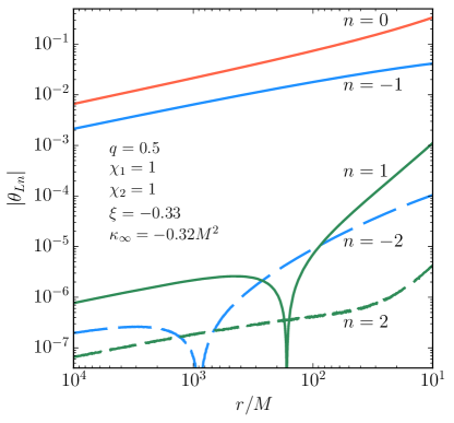
Figure 3: The magnitudes of the five largest coefficients $\theta_{Ln}$ in the series expansion of Eq. (26) as a function of binary separation $r$ for a binary with mass ratio $q=0.5$, maximal dimensionless spins $\chi_{1}=\chi_{2}=1$, projected effective spin $\xi=-0.33$, and asymptotic projected total spin $\kappa_{\infty}=-0.32M^{2}$. The $n=0$ and $n=-1$ coefficients shown by the solid red and blue curves remain the two largest coefficients throughout the inspiral, while the $n=+1,+2,-2$ coefficients, shown by the solid green, dashed green, and dashed blue curves respectively, remain less than 1% of the two dominant curves until just before the final separation $r=10M$.

We show the five largest coefficients $\theta_{Ln}$ for $n=0,\pm 1,\pm 2$ during the inspiral of a different binary from $r=10^{4}M$ to $10M$ in Fig. 3. The parameters for this binary, listed in the caption to the figure, were chosen such that the binary passes through a nutational resonance at $r\simeq 481M$. Such nutational resonances are the focus of Sections IV and V; the same binary is also shown in Figs. 4 and 5. This binary differs from the one shown in Fig. 2 in that it does not pass through any discontinuities in $\alpha$, but shares the common feature that the $n=-1,0$ terms are dominant through most of the inspiral. For such binaries, the precession of $\mathbf{L}$ can be modeled to $\sim 1\%$ accuracy using just the two dominant terms in Eq. (26) whose coefficients vary smoothly on the radiation-reaction timescale. This suggests that precession averaging can provide computational savings for the evolution of $\mathbf{L}$ during an inspiral similar to those obtained for the evolution of the total angular momentum $J$ demonstrated in our previous work Kesden et al. (2015); Gerosa et al. (2015a).

Our new expansion in Eq. (26) can also be used to calculate the evolution of the total angular momentum $\mathbf{J}(t)$ in our inertial $xyz$ frame. If the rate at which angular momentum is radiated is related to the orbital angular momentum by Eq. (16), our expansion implies that

$$\frac{d\mathbf{J}_{\perp}}{dt} =-\frac{32}{5}\left(\frac{r}{M}\right)^{-4}\frac{\eta\mathbf{L}_{\perp}}{M}$$

$$=\frac{dL}{dt}\sum_{n=-\infty}^{+\infty}\theta_{Ln}\{\cos[(\Omega-n\omega)t]\mathbf{\hat{x}}+\sin[(\Omega-n\omega)t]\mathbf{\hat{y}}\}~{}.$$ (30)

If we integrate this expression on the precession timescale, holding fixed the amplitudes and frequencies varying on the longer radiation-reaction timescale, we find a similar expansion for the perpendicular component of the total angular momentum,

$$\mathbf{J}_{\perp}(t)=J\sum_{n=-\infty}^{+\infty}\theta_{Jn}\{\sin[(\Omega-n\omega)t]\mathbf{\hat{x}}-\cos[(\Omega-n\omega)t]\mathbf{\hat{y}}\}~{},$$ (31)

where the coefficients in the two expansions of Eqs. (26) and (31) are proportional to each other:

$$\frac{\theta_{Jn}}{\theta_{Ln}}=\frac{1}{J}\frac{dL}{dt}\left(\frac{1}{\Omega-n\omega}\right)\propto\frac{t_{\rm pre}}{t_{\rm RR}}\propto\left(\frac{r}{M}\right)^{-3/2}.$$ (32)

This agrees with the earlier finding that for simple precession, the total angular momentum $\mathbf{J}$ precesses about a cone with opening angle $\theta_{J}\propto(r/M)^{-2}$ much less than the opening angle $\theta_{L}\propto(r/M)^{-1/2}$ of the cone about which the orbital angular momentum $\mathbf{L}$ precesses Apostolatos et al. (1994). Eq. (32) reveals that $\theta_{Jn}$ diverges for $\Omega=n\omega$, mathematically equivalent to $\alpha=2\pi n$ from our definitions of the precession and nutation frequencies in Sec. II. This condition, which we call a nutational resonance, has potentially profound implications for the evolution of $\mathbf{J}$ which we explore in the next section.

IV Nutational Resonances

At a nutational resonance, the arguments of the sinusoids in the $n=\Omega/\omega$ term in Eq. (III) vanish, implying that this term corresponds to constant emission of angular momentum in the $x$ direction. This emission will cause the precession-averaged total angular momentum $\langle\mathbf{J}\rangle$ to tilt towards the $x$ axis and away from its initial direction which defined the $z$ axis. This tilting behavior will not continue indefinitely, because the precession frequency $\Omega$ and nutation frequency $\omega$ are both evolving on the radiation-reaction timescale $t_{\rm RR}$. A generic binary will not be in a nutational resonance ($\Omega/\omega$ will not be an integer), but as it inspirals towards merger it may pass through one or more of such resonances. At each passage through a nutational resonance, the precession-averaged total angular momentum $\langle\mathbf{J}\rangle$ will tilt by some angle $\theta_{\rm tilt}$, providing a randomly oriented “kick” of magnitude $J\theta_{\rm tilt}$ to $\mathbf{J}_{\perp}$ in an inertial frame. These kicks will accumulate throughout the inspiral causing $\langle\mathbf{J}\rangle$ to random walk away from its initial direction at large separations set by binary formation. Whether these tilts are astrophysically relevant or lead to detectable GW signatures depends on both the magnitudes of the tilt angles $\theta_{\rm tilt}$ and the frequency with which binaries encounter nutational resonances. We will derive an analytic estimate of the tilt angle $\theta_{\rm tilt}$ in this section, then use this estimate to explore the distribution of tilt angles as a function of binary parameters in Sec. V.

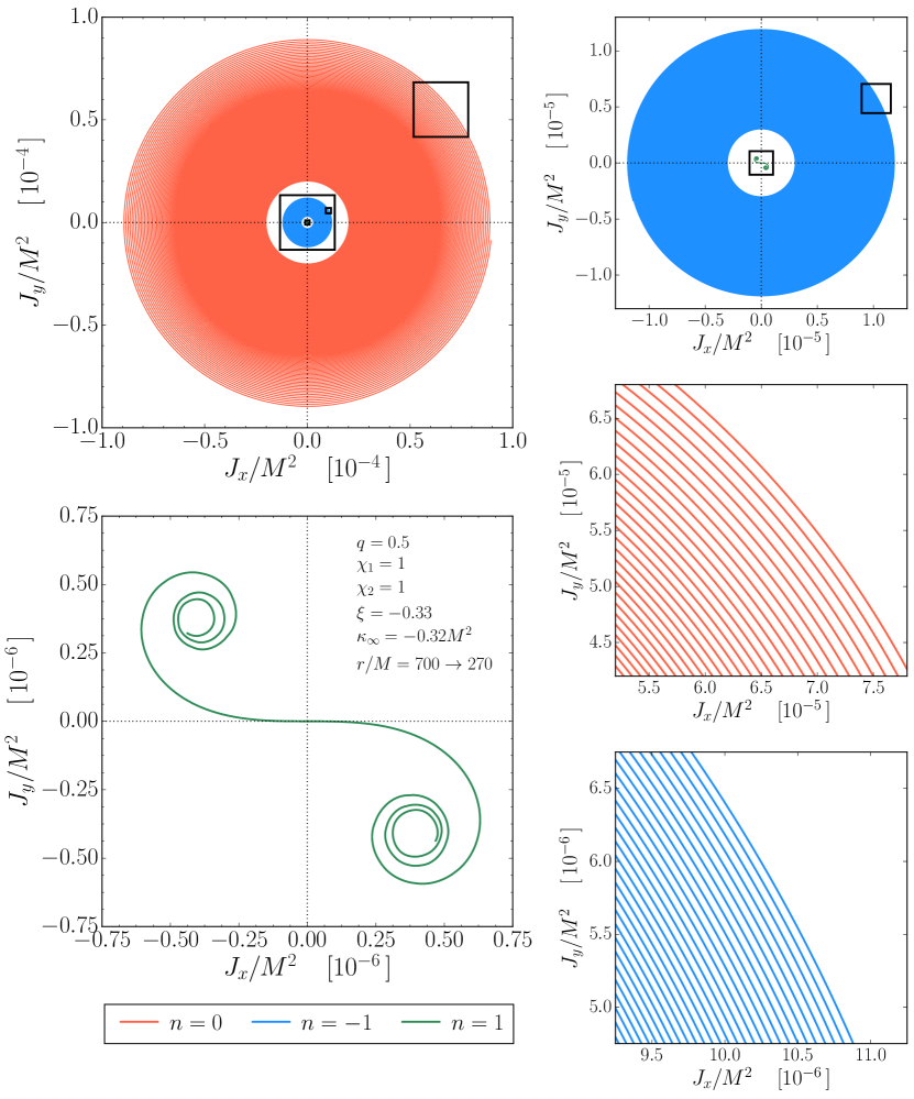
Figure 4: The evolution of $\mathbf{J}_{\perp}$, the component of the total angular momentum in the $xy$ plane, as binary black holes with mass ratio $q=0.5$, maximal dimensionless spins $\chi_{1}=\chi_{2}=1$, and projected effective spin $\xi=-0.33$ inspiral from $r=700M$ to $r=270M$. The binary encounters a $n=1$ nutational resonance ($\Omega=\omega$) at $r\simeq 481M$ when the magnitude of the total angular momentum $J\simeq 4.56M$. The direction of $\mathbf{J}$ at this point in the inspiral defines the $z$ axis. The red, blue, and green curves show numerical integration of the $n=\{0,-1,+1\}$ terms respectively in the expansion of Eq. (III). The top left panel shows the largest view, while the top right and middle right panels show two insets to this figure. The bottom left and bottom right panels show the two insets to the top right panel. The bottom left panel most clearly shows that the resonant $n=1$ term shown by the green curve is tilted as it passes through resonance.

We show an example of BBHs passing through a $n=1$ nutational resonance in Fig. 4. We integrate Eq. (III) numerically backwards and forwards in time from the resonance at $r\simeq 481M$, defining the $z$ axis to point in the direction of the precession-averaged total angular momentum $\langle\mathbf{J}\rangle$ at this binary separation. We show the dominant non-resonant $n=0$ and $n=-1$ terms with red and blue curves respectively, while the resonant $n=1$ term is shown by the green curve. On the precession timescale, the non-resonant $n=0$ and $n=-1$ terms trace circles in the $xy$ plane with radii $J|\theta_{J0}|$ and $J|\theta_{J,-1}|$ and frequencies $\Omega$ and $\Omega+\omega$, consistent with the expansion for $\mathbf{J}_{\perp}$ given in Eq. (31). On the radiation-reaction timescale, these curves spiral outwards as $\theta_{Jn}$ increase in magnitude as the binary separation $r$ decreases from $700M$ to $270M$.

The resonant $n=1$ term exhibits qualitatively different behavior, in addition to being much smaller in magnitude consistent with the hierarchy of coefficients shown in Fig. 3. At large separations, where the precession frequency $\Omega$ and nutation frequency $\omega$ have not quite achieved resonance, the $n=1$ term precesses in small circles with radii $J|\theta_{J1}|$ and very small frequency $\Omega-\omega$. This is shown in the top left corner of the bottom left panel of Fig. 4. As the binary approaches resonance, the angular momentum loss due to this term comes to point in a fixed direction on the precession timescale (along the $x$ axis). Next, the binary passes through resonance when the green curve reaches the origin at $J_{x}=J_{y}=0$. Finally, the $n=1$ term resumes precession with frequency $\Omega-\omega$ (now negative) along circles with radii $J|\theta_{J1}|$ as shown in the bottom right corner of the bottom left panel of Fig. 4. The axes about which the $n=1$ term precesses before and after resonance are displaced with respect to each other, corresponding to a tilt in the precession-averaged total angular momentum $\langle\mathbf{J}\rangle$.

We can estimate the magnitude of this tilt by Taylor expanding the resonant term in Eq. (III) about the resonance and integrating analytically. We begin with the frequency of the resonant term ,

$$\Omega-n\omega\simeq\left[\frac{d(\Omega-n\omega)}{dL}\right]_{0}(L-L_{0})=sD^{2}t~{},$$ (33)

where the total derivative of the frequency with respect to the magnitude of the orbital angular momentum is evaluated at resonance where $L=L_{0}$. In this expression, we have also defined the binary to pass through resonance at $t=0$ and two constants

$$s \equiv{\rm sgn}\left(\frac{d\alpha}{dL}\frac{dL}{dt}\frac{1}{\tau}\right)~{},$$ (34)

$$D \equiv\left|\frac{d\alpha}{dL}\frac{dL}{dt}\frac{1}{\tau}\right|^{1/2}\propto\frac{1}{\sqrt{t_{\rm RR}t_{\rm pre}}}\propto\left(\frac{r}{M}\right)^{-13/4}.$$ (35)

Eqs. (33) and (29) imply that the phase near resonance is given by

$$\psi_{n}=\int_{0}^{t}(\Omega-n\omega)~{}dt^{\prime}\simeq\frac{1}{2}sD^{2}t^{2}~{}.$$ (36)

Inserting this phase into the arguments of the sinusoids of the resonant term in Eq (III), we find that

$$\frac{d\mathbf{J}_{\perp n}}{dt}=\frac{dL}{dt}\theta_{Ln}\left[\cos\left(\frac{1}{2}D^{2}t^{2}\right)\mathbf{\hat{x}}+s\sin\left(\frac{1}{2}D^{2}t^{2}\right)\mathbf{\hat{y}}\right]$$ (37)

Integrating Eq. (37) leads to

$$\mathbf{J}_{\perp n}=\frac{\sqrt{2}}{D}\frac{dL}{dt}\theta_{Ln}\left[\mathcal{C}\left(\frac{Dt}{\sqrt{2}}\right)\mathbf{\hat{x}}+s\mathcal{S}\left(\frac{Dt}{\sqrt{2}}\right)\mathbf{\hat{y}}\right]$$ (38)

where $\mathcal{C}(x)$ and $\mathcal{S}(x)$ are the Fresnel integrals

$$\mathcal{C}(x) \equiv\int_{0}^{x}\cos t^{2}~{}dt~{},$$ (39a)

$$\mathcal{S}(x) \equiv\int_{0}^{x}\sin t^{2}~{}dt~{}.$$ (39b)

Eq. (38) indicates that the resonant term $\mathbf{J}_{\perp n}$ can be approximated as an Euler spiral. We compare this Euler spiral to a numerical integration of the resonant term in Eq. (III) in Fig. 5.

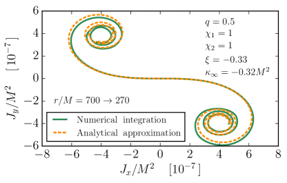
Figure 5: A comparison between numerical integration of the resonant term in Eq. (III) for the nutational resonance depicted in Fig. 4 and our analytical approximation given by Eq. (38). The agreement is excellent; the symmetric Euler spiral shown by the dashed orange curve nearly perfectly describes the numerical integration shown by the solid green curve despite the significant changes in $L$ and $J$ as the binary inspirals from $r=700M$ to $r=270M$.

The Fresnel integrals have limiting values

$$\lim_{x\to\pm\infty}\mathcal{C}(x),\mathcal{S}(x)=\pm\sqrt{\pi/8}$$ (40)

which allow us to estimate the total shift

$$\Delta\mathbf{J}_{\perp n}\equiv\mathbf{J}_{\perp n}(\infty)-\mathbf{J}_{\perp n}(-\infty)$$ (41)

in the precession-averaged total angular momentum relative to its direction at resonance as a binary passes through a nutational resonance. This in turn implies that $\mathbf{J}$ tilts by an angle

$$\theta_{\rm tilt} =\frac{|\Delta\mathbf{J}_{\perp n}|}{J}=\frac{(2\pi)^{1/2}}{JD}\frac{dL}{dt}\theta_{Ln}$$

$$\propto\left(\frac{t_{\rm{pre}}}{t_{\rm{RR}}}\right)^{1/2}\theta_{Ln}\propto\left(\frac{r}{M}\right)^{-5/4}~{}.$$ (42)

For the nutational resonance shown in Fig. 5, the total shift $\Delta\mathbf{J}_{\perp n}$ predicted by Eq. (41) agrees with the numerical result obtained by integrating Eq. (III) to better than 1%. This justifies our use of Eq. (IV) in the next section to estimate how the precession-averaged total angular momentum $\langle\mathbf{J}\rangle$ tilts as BBHs encounter nutational resonances during their inspirals.

V Distribution of Nutational Resonances

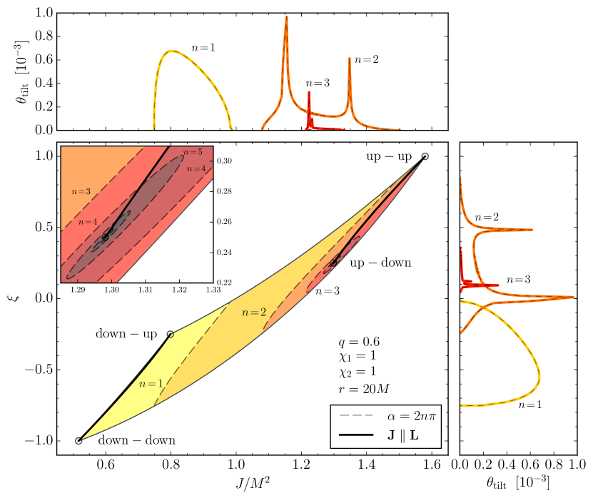
Figure 6: Central panel: A contour plot of the precession angle $\alpha$ as a function of the magnitude of the total angular momentum $J$ and the projected effective spin $\xi$ for BBHs with mass ratio $q=0.6$, dimensionless spin magnitudes $\chi_{1}=\chi_{2}=1$, and binary separation $r=20M$. The colored region shows the allowed values of $J$ and $\xi$ for these parameters, with the three cusps on the boundaries corresponding to the up-up, down-up, and down-down configurations. The thin dashed lines indicate nutational resonances ($\alpha=2\pi n$ for integer $n$). The inset shows parameter space near the unstable up-down configuration where $\alpha\to\infty$. The solid black lines show binaries for which $\mathbf{J}$ and the orbital angular momentum $\mathbf{L}$ are parallel at $S=S_{-}$, implying that $\alpha$ is undefined. The value of $\alpha$ along contours crossing these lines changes by $\pm 2\pi$. Top and right panels: The tilt angle $\theta_{\rm tilt}$ along the $\alpha=2\pi n$ nutational resonance contours as functions of $J$ and $\xi$ respectively. The spikes on these curves correspond to parameters for which $d\alpha/dL\to 0$ implying $\theta_{\rm tilt}\to\infty$ by Eqs. (35) and (IV).

In this section, we investigate how often BBHs encounter nutational resonances as they inspiral towards merger from the large separations at which they form. As the condition $\alpha=2\pi n$ for integer $n$ defines a nutational resonance, we begin by calculating $\alpha$ according to Eq. (13). Although the parameter space of all BBHs with given masses, spin magnitudes, and binary separation is four dimensional (corresponding to the two BBH spin directions), two of these dimensions can be specified by a global rotation of the system about $\mathbf{J}$ and the precessional phase, neither of which affect $\alpha$ which varies on the radiation-reaction timescale. For these BBHs (for which $L$ is fixed), $\alpha$ is purely function of $J$ and $\xi$ for allowed values of these parameters. We show a contour plot of $\alpha$ for these allowed values in Fig. 6, where the contour lines $\alpha=2\pi n$ identify nutational resonances. The largest allowed value of the magnitude of the total angular momentum $J$ is $J_{\rm max}=L+S_{1}+S_{2}$ and occurs for the “up-up” configuration in which both spins $\mathbf{S}_{1}$ and $\mathbf{S}_{2}$ are aligned with the orbital angular momentum $\mathbf{L}$. Since $L>S_{1}+S_{2}$ for these BBH masses and spins, the smallest allowed value of $J$ is $J_{\rm min}=L-S_{1}-S_{2}$ and occurs for the “down-down” configuration in which $\mathbf{S}_{1}$ and $\mathbf{S}_{2}$ are anti-aligned with $\mathbf{L}$. The boundaries of the allowed region in the $J-\xi$ plane are defined by two paths connecting the “up-up” and “down-down” configurations. The first of these paths, $\xi_{\rm max}(J)$, connects the maxima of the effective potential $\xi_{+}(S)$ given by Eq. (II). This path includes the “down-up” configuration in which the spin $\mathbf{S}_{1}$ of the more massive black hole is anti-aligned with $\mathbf{L}$ while the spin $\mathbf{S}_{2}$ of the less massive black hole is aligned. The second path $\xi_{\rm min}(J)$ connects the minima of the effective potential $\xi_{-}(S)$. The allowed region in Fig. 6 consists of those BBHs for which $J_{\rm min}\leq J\leq J_{\rm max}$ and $\xi_{\rm min}(J)\leq\xi\leq\xi_{\rm max}(J)$.

The $n=1$ and $n=2$ contours in Fig. 6 connect points on the $\xi_{\rm min}(J)$ and $\xi_{\rm max}(J)$ curves that constitute the boundaries of the allowed region. Because these boundaries correspond to extrema of the effective potential $\xi_{\pm}(S)$ (what Schnittman Schnittman (2004) described as spin-orbit resonances), $S$ does not oscillate, $\Omega_{z}(S)$ given by Eq. (II) is a constant on the precession timescale, and the coefficients $\theta_{Ln}$ given by Eq. (27) vanish for $n\neq 0$. The tilt angle $\theta_{\rm tilt}$ given by Eq. (IV) is proportional to $\theta_{Ln}$ and thus must similarly vanish for $n\neq 0$. The $n=1$ and $n=2$ contours in Fig. 6 are monotonic functions of both $J$ and $\xi$, so either of these quantities can be used to parametrize the curves. We show $\theta_{\rm tilt}(J)$ and $\theta_{\rm tilt}(\xi)$ in the top and right panels of Fig. 6. As expected, $\theta_{\rm tilt}$ vanishes at the endpoints of these curves (the Schnittman spin-orbit resonances) for both nutational resonances. The curves $\theta_{\rm tilt}(J)$ and $\theta_{\rm tilt}(\xi)$ are smooth functions for the $n=1$ resonance, reaching a maximum $\theta_{\rm tilt}\simeq 7\times 10^{-4}$ somewhere in the interior of the allowed region. The corresponding curves for the $n=2$ resonance show two sharp spikes where the tilt angle appears to diverge. These spikes are artifacts of the approximations used in Section IV and occur where $d\alpha/dL$ and thus $D$ given by Eq. (35) vanish. Since $D$ appears in the denominator of Eq. (IV) for $\theta_{\rm tilt}$, the tilt angle correspondingly diverges. Physically, points for which both $\alpha=2\pi n$ and $d\alpha/dL=0$ correspond to BBHs that are in nutational resonances and remain in these resonances as they inspiral on the radiation-reaction timescale. In practice, the quadratic term in the Taylor expansion of Eq. (33) will be non-vanishing for these BBHs, implying that the phase $\psi_{n}$ given by Eq. (36) will by cubic rather than quadratic in $t$. An order-of-magnitude analysis for these BBHs suggests that $\theta_{\rm tilt}$ will be proportional to $(r/M)^{-1}$ rather than $(r/M)^{-5/4}$ as in Eq. (IV), implying somewhat larger but still finite tilts.

The contours for the $n>2$ resonances in Fig. 6 exhibit more complicated behavior. The $n=3$ contour begins on the $\xi_{\rm min}(J)$ boundary, then curves up and to the right until it encounters the solid black curve connecting the “up-up” and “up-down” configurations identifying those BBHs for which the total spin $\mathbf{S}$ and orbital angular momentum $\mathbf{L}$ are aligned at $S=S_{-}$. For these BBHs, the total angular momentum $\mathbf{J}=\mathbf{L}+\mathbf{S}$ is also aligned with $\mathbf{L}$ implying that $\alpha$ is undefined as was previously discussed in Section III Trifirò et al. (2016). Crossing this solid black curve causes $\alpha$ to change discontinuously by $2\pi$, transforming our $n=3$ contour into an $n=4$ contour, another nutational resonance. For these BBH masses and spins, the “up-down” configuration defining one endpoint of the $\alpha$ discontinuity curve lies in the interior rather than on the $\xi_{\rm min}(J)$ boundary of the allowed region in the $J-\xi$ plane. This occurs for binary separations $r_{\rm ud-}<r<r_{\rm ud+}$, where the limits

$$r_{\rm ud\pm}=\frac{(\sqrt{\chi_{1}}\pm\sqrt{q\chi_{2}})^{4}}{(1-q)^{2}}M$$ (43)

define the range for which the “up-down” configuration is unstable to precession to large spin misalignments Gerosa et al. (2015b). For these unstable “up-down” configurations, the nutation period $\tau$ is infinite, just as it will take an infinite amount of time for a particle moving in a one-dimensional potential to reach a local maximum (unstable equilibrium point) which it has just enough energy to access. Since the precession frequency $\Omega$ remains finite as one approaches the unstable “up-down” configuration while the nutation period $\tau$ diverges, the precession angle $\alpha=\Omega\tau$ also becomes infinite. This implies that as one approaches the point in the $J-\xi$ plane corresponding to the unstable “up-down” configuration, one will encounter nutational resonances $\alpha=2\pi n$ for arbitrarily large values of $n$. This is what we see in the inset to the central panel of Fig. 6: the contour lines corresponding to nutational resonances spiral inwards towards the “up-down” configuration, with $n$ increasing by an integer each time the solid line marking the $\alpha$ discontinuity is crossed. Although $n$ diverges along this spiral, the tilt angle $\theta_{\rm tilt}$ approaches zero because the BBH spends an increasing fraction of the nutation period with $\mathbf{L}$ closely aligned with $\mathbf{J}$, implying little tilt in $\langle\mathbf{J}\rangle$ for radiation reaction described by the quadrupole formula of Eq. (16).

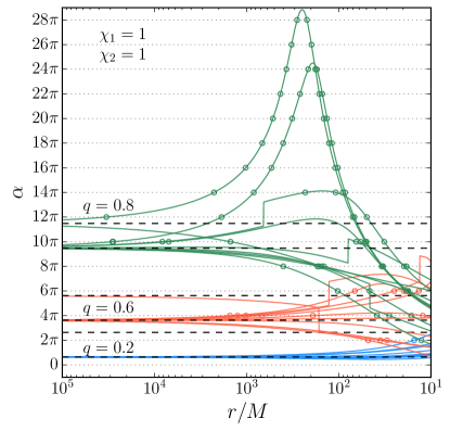
Figure 7: The angle $\alpha$ by which the orbital angular momentum $\mathbf{L}$ and total angular momentum $\mathbf{J}$ precess about the $z$ axis during a nutation period $\tau$ as a function of binary separation $r$ for 30 different binaries with randomly oriented maximal spins ($\chi_{i}=1$). The 10 green, red, and blue curves correspond to BBHs with mass ratios $q=0.8$, 0.6, and 0.2 respectively. The dashed black lines show the asymptotic values $\alpha_{\infty\pm}$ as $r\to\infty$ for the three mass ratios. The dotted black lines show the resonance condition $\alpha=2\pi n$, while the colored circles indicate separations where the BBHs encounter nutational resonances.

Now that we understand which BBHs are in nutational resonances at a given binary separation (for example, $r=20M$ in Fig. 6), we can examine when BBHs encounter these resonances as their separation decreases as they inspiral towards merger. In Fig. 7, we show $\alpha(r)$ for 30 BBHs (10 each for mass ratios $q=0.8$, 0.6, and 0.2) with randomly oriented maximal spins as they inspiral from $r=10^{5}M$ to a final separation $r=10M$. At large separations, we see that the precession angles $\alpha$ asymptote to one of two different values for each of the three mass ratios; these asymptotic values are shown by the dashed black lines in Fig. 7. This surprising result can be understood by recognizing that the lower PN order spin-orbit coupling dominates over the high-order spin-spin coupling in the limit $r\to\infty$. In this limit, the angles between the orbital angular momentum $\mathbf{L}$ and the BBH spins $\mathbf{S}_{1}$ and $\mathbf{S}_{2}$ are fixed to their asymptotic values $\theta_{1\infty}$ and $\theta_{2\infty}$, $\mathbf{L}$ and the total angular momentum $\mathbf{J}$ are both nearly aligned with the $z$ axis, and the two spins precess about this axis with respective frequencies Apostolatos et al. (1994); Kidder (1995)

$$\Omega_{1} =\frac{(4+3q)\eta}{2M}\left(\frac{r}{M}\right)^{-5/2},$$ (44a)

$$\Omega_{2} =\frac{(4+3/q)\eta}{2M}\left(\frac{r}{M}\right)^{-5/2}.$$ (44b)

Unless the BBHs masses are precisely equal, the mass ratio $q<1$ and the spin of the less massive black hole precesses faster ($\Omega_{2}>\Omega_{1}$). If the components of $\mathbf{S}_{1}$ and $\mathbf{S}_{2}$ perpendicular to the $z$ axis are aligned at $t=0$, they will first realign (return to their initial relative orientations) after a nutation period $\tau$. Over this interval, the faster spin $\mathbf{S}_{2}$ will precess about $z$ by an additional $2\pi$ radians compared to the slower spin $\mathbf{S}_{1}$:

$$(\Omega_{2}-\Omega_{1})\tau=2\pi~{}.$$ (45)

In order for $\mathbf{J}$ to remain nearly aligned with the $z$ axis ($\theta_{J}\ll\theta_{L}$), $\mathbf{L}$ must have a component $\mathbf{L}_{\perp}$ in the $xy$ plane anti-aligned with the component $\mathbf{S}_{\perp}$ of the total spin in this plane. If $S_{1\perp}=S_{1}\sin\theta_{1\infty}>S_{2\perp}=S_{2}\sin\theta_{2\infty}$, $\mathbf{S}$ and thus $\mathbf{L}$ will precess about the $z$ axis over the nutation period $\tau$ by an angle

$$\alpha_{\infty-}=\Omega_{1}\tau=\frac{2\pi\Omega_{1}}{\Omega_{2}-\Omega_{1}}=\frac{2\pi q(4+3q)}{3(1-q^{2})}~{},$$ (46)

which we have derived using Eqs. (44) and (45). If $S_{1}\sin\theta_{1\infty}<S_{2}\sin\theta_{2\infty}$, the asymptotic precession angle will instead be given by

$$\alpha_{\infty+}=\Omega_{2}\tau=\alpha_{\infty-}+2\pi=\frac{2\pi(4q+3)}{3(1-q^{2})}~{}.$$ (47)

If the BBHs have isotropically oriented spins with magnitudes $S_{1}$ and $S_{2}$, the fraction of binaries for which $\alpha$ asymptotes to $\alpha_{\infty+}$ for $S_{1}>S_{2}$ is

$$f_{+}=\frac{|S_{1}^{2}-S_{2}^{2}|}{4S_{1}S_{2}}[\sinh(2\cosh^{-1}C)-2\cosh^{-1}C]~{},$$ (48)

while for $S_{1}<S_{2}$ it is

$$f_{+}=\frac{|S_{1}^{2}-S_{2}^{2}|}{4S_{1}S_{2}}[\sinh(2\sinh^{-1}C)+2\sinh^{-1}C]~{},$$ (49)

where in both expressions $C\equiv S_{1}/|S_{1}^{2}-S_{2}^{2}|^{1/2}$. For the three mass ratios $q=\{0.8,0.6,0.2\}$ in Fig. 7, Eqs. (46) through (48) imply $\alpha_{\infty-}=\{9.48\pi,3.63\pi,0.64\pi\}$, $\alpha_{\infty+}=\{11.48\pi,5.63\pi,2.64\pi\}$, and $f_{+}=\{0.15,0.0444,5.34\times 10^{-4}\}$. These values are consistent with the horizontal dashed lines in Fig. 7 and that $\{2/10,1/10,0/10\}$ of the binaries asymptote to $\alpha_{\infty+}$ for $q=\{0.8,0.6,0.2\}$.

As the BBHs in Fig. 7 inspiral from large separations towards merger, they encounter nutational resonances marked by small colored circles whenever $\alpha=2\pi n$. BBHs with mass ratios for which $\alpha_{\infty\pm}$ is close to an integer multiple of $2\pi$ are most likely to encounter nutational resonances at large binary separations. We also see several discontinuous jumps in $\alpha$ by $\pm 2\pi$ corresponding to configurations in which the orbital angular momentum $\mathbf{L}$ and total angular momentum $\mathbf{J}$ are either aligned or anti-aligned at $S=S_{+}$ or $S_{-}$. According to Eq. (43), the BBHs with mass ratios $q=\{0.8,0.6,0.2\}$ in Fig. 7 enter the regime where the “up-down” configuration is unstable for binary separations $r<r_{\rm ud+}\simeq\{322M,62M,6.85M\}$. The large peak values $\alpha>24\pi$ occurring at $r\lesssim r_{\rm ud+}$ for two of the $q=0.8$ binaries in Fig. 7 result from close approaches in the $J-\xi$ plane to the unstable “up-down” configuration for which $\alpha\to\infty$. The key point to take away from Fig. 7 is that most binaries with large spins and $q\gtrsim 0.6$ encounter one or more nutational resonances during their inspiral, and many of these resonances occur at $r<100M$ where tilts are comparatively large and GWs for solar-mass BBHs are emitted at frequency detectable by ground-based GW observatories like LIGO.

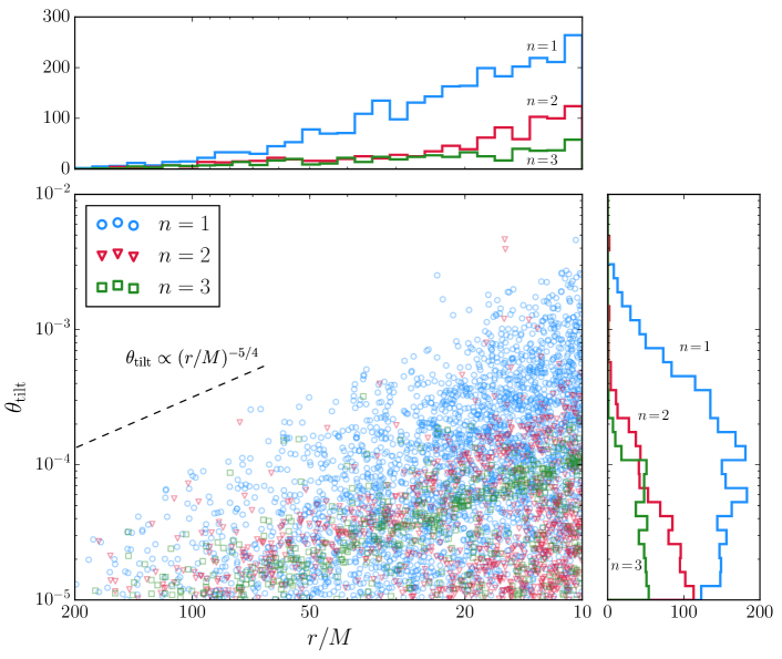
Figure 8: Distribution of nutational resonances as a function of binary separation $r$ and tilt angle $\theta_{\rm tilt}$ for $5\times 10^{4}$ binaries with isotropically oriented spins and flat distributions of mass ratios and dimensionless spins in the ranges $0.1<q<1$ and $0.1<\chi_{i}<1$. The central panel is a scatter plot in which each blue circle, red triangle, and green square corresponds to a $n=\{1,2,3\}$ nutational resonance encountered by one of the BBHs. The dashed black line $\theta_{\rm tilt}\propto(r/M)^{-5/4}$ shows that the scaling of the largest tilt angles with binary separation agrees with the analytic prediction of Eq. (IV). The top and right panels show histograms generated by binning this scatter plot of the nutational resonances as functions of binary separation $r$ and tilt angle $\theta_{\rm tilt}$ for each value of $n$. The binaries encounter a total of $N=\{2717,923,517\}$ resonances for $n=\{1,2,3\}$ with $\theta_{\rm tilt}>10^{-5}$ in the range $200M>r>10M$, implying that $\sim 8.3\%$ of the BBHs encounter such resonances.

Having examined how $\alpha$ evolves with binary separation for the 30 binaries show in Fig. 7, we now broaden our sample to $5\times 10^{4}$ binaries with a flat distribution of mass ratios in the range $0.1<q<1$ and isotropic spins with a flat distribution of dimensionless magnitudes in the range $0.1<\chi_{i}<1$. In Fig. 8, we show all of the nutational resonances with $|n|\leq 3$ and $\theta_{\rm tilt}>10^{-5}$ encountered by these binaries as they inspiral from $r=200M$ to $r=10M$. No resonances with $n\leq 0$ were observed, suggesting that such resonances may not exist although we have not found a mathematical proof of their non-existence. A total of 4157 nutational resonances were found during these $5\times 10^{4}$ inspirals (an incidence of 8.3%), with most occurring at $r\lesssim 50M$ as shown by the histogram in the top panel of Fig. 8. The previous sample shown in Fig. 7 suggests that BBHs with comparable masses should account for the majority of these nutational resonances because the steeper slopes of their $\alpha(r)$ curves should increase the probability that they cross an $\alpha=2\pi n$ line signaling a nutational resonance. There are 2717 $n=1$ resonances (65.4% of the total) with a broad range of tilts, including a tail extending to $\theta_{\rm tilt}>10^{-3}$ for $r\lesssim 20M$ as shown by the histogram in the right panel of Fig. 8. The largest tilt angles appears to scale with binary separation as $\theta_{\rm tilt}\propto(r/M)^{-5/4}$ consistent with the analytic estimate of Eq. (IV). The 923 $n=2$ and 517 $n=3$ resonances constitute smaller fractions of the total (22.2% and 12.4% respectively) and generally lead to smaller tilts $\theta_{\rm tilt}<10^{-3}$. Although there may be finely tuned resonances missing from our sample with even larger tilts (such as those with $d\alpha/dL=0$ indicated by the spikes in the top and right panels of Fig. 6), the results shown in Fig. 8 suggest that tilts from exact resonances at binary separations $r>10M$ are too small to have significant astrophysical consequences or detectable GW signatures. However, we will show in the next section that the large tilts associated with transitional precession Apostolatos et al. (1994) can be interpreted as a consequence of an approximate $n=0$ nutational resonance.

VI Transitional precession as an approximate nutational resonance

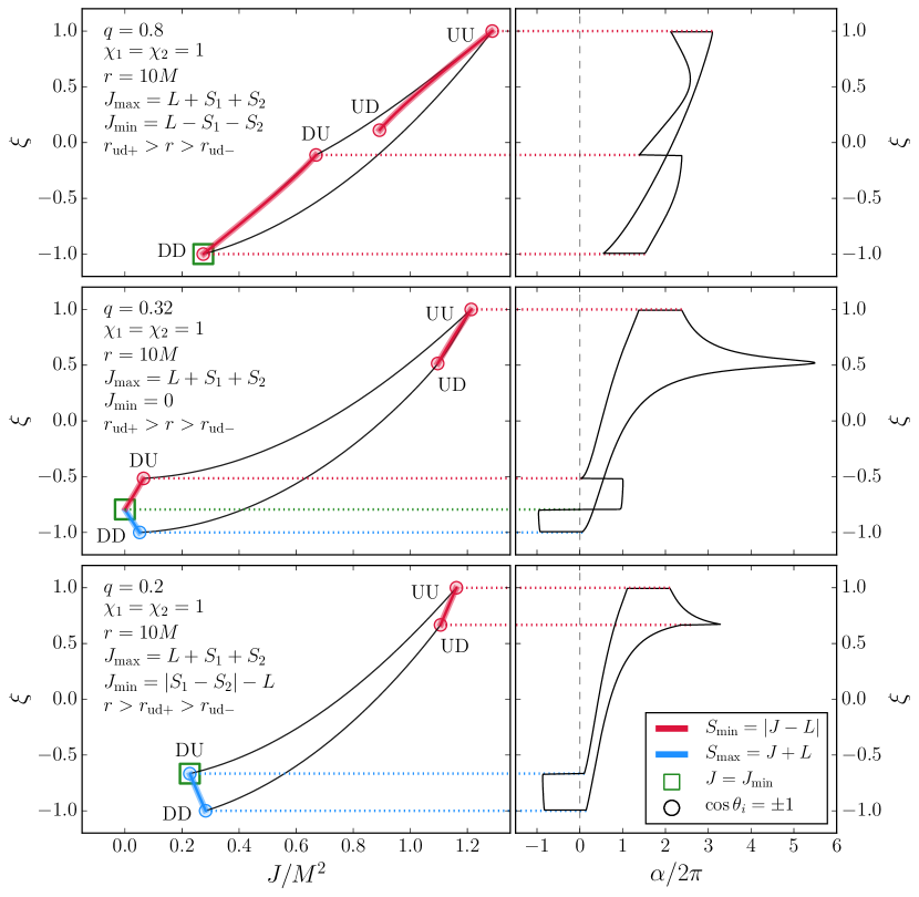
Figure 9: Left panels: Boundaries of the allowed region in the $J-\xi$ plane for BBHs with binary separations of $r=10M$, maximal spin magnitudes, and mass ratios of $q=0.8$ (top panel), 0.32 (middle panel), and 0.2 (bottom panel). The BBHs along the red curves have the orbital angular momentum $\mathbf{L}$ aligned with the total angular momentum $\mathbf{J}$ once per nutation period, when $S=S_{-}=S_{\rm min}=|J-L|$, while the BBHs along the blue curves have $\mathbf{L}$ aligned with $\mathbf{J}$ once per nutation period when $S=S_{+}=S_{\rm max}=J+L$. The four circles in each panel indicate the BBHs for which the spins $\mathbf{S}_{i}$ are both either aligned or anti-aligned with $\mathbf{L}$; the circles labeled “UU”, “UD”, “DU”, and “DD” correspond to the up-up, up-down, down-up, and down-down configurations respectively. The green squares indicate the minimum allowed value of $J$ for each mass ratio. Right panels: The precession angle $\alpha$ over a nutation period $\tau$ as a function of the projected effective spin $\xi$ along the boundaries of the allowed regions. The horizontal dotted lines indicate values of $\xi$ at which the red and blue curves intersect the boundaries, while the vertical dashed line indicates $\alpha=0$.

The tilt angles $\theta_{\rm tilt}$ shown in Fig. 8 are disappointingly small if we ever hope to measure their observational consequences. The coefficients $\theta_{Ln}$ shown in Fig. 3 are several orders of magnitude larger for $n=0$ and $n=-1$ than the other coefficients, suggesting from Eq. (IV) that the tilt angles at $n=0$ or $n=-1$ nutational resonances would be similarly larger, perhaps even of order unity, if such resonances could be found. Our investigation of the $\alpha=2\pi n$ contours in Fig. 6 suggests that if $n=0$ or $n=-1$ contours exist, they will intersect the boundaries of the allowed region in the $J-\xi$ plane. To test this possibility, we plot these boundaries and the value of $\alpha$ along them for BBHs with maximal spins, binary separations of $r=10M$, and three different mass ratios $q=\{0.8,0.32,0.2\}$ in Fig. 9. These three mass ratios provide examples of the three alternative values of $J_{\rm min}$, the minimum allowed magnitude of the total angular momentum Gerosa et al. (2015a). If $L>S_{1}+S_{2}$, the minimum allowed magnitude of $\mathbf{J}=\mathbf{L}+\mathbf{S}_{1}+\mathbf{S}_{2}$ is $L-S_{1}-S_{2}$ as is the case for $q=0.8$, $\chi_{1}=\chi_{2}=1$, and $r=10M$ as seen in the top panel of Fig. 9. This value of $J_{\rm min}$, indicated by the green square, corresponds to the “down-down” configuration indicated by one of the four circles showing the four configurations in which the BBH spins $\mathbf{S}_{i}$ are both either aligned or anti-aligned with $\mathbf{L}$. The right side of this panel shows $\alpha(\xi)$ as we circulate around the boundary of the allowed region in the $J-\xi$ plane. The continuous curve connecting $\xi=\pm 1$ corresponds to the right edge of the allowed region, while the other two curves correspond to the left edge of the allowed region. At each of the three circles on the boundary of the allowed region (the “up-up”, “down-up”, and “down-down” configurations), the value of $\alpha$ changes discontinuously by $\pm 2\pi$ because of the coordinate discontinuity discussed previously. As $r_{\rm ud-}<r<r_{\rm ud+}$ according to Eq. (43) for this choice of parameters, the unstable “up-down” configuration lies in the interior of the allowed region and thus does not lead to a discontinuity in $\alpha$ along the boundary. It is important to note that the red curve connecting the “down-up” and “down-down” configurations denoting BBHs for which $\alpha$ is undefined lies in the interior of the allowed region, although it is so close to boundary as to appear indistinguishable from it in this figure. The red and blue curves in the middle and bottom panels are also in the interior of the allowed region despite their close proximity to the boundary.

We now examine the middle panel of Fig. 9 which differs from the top panel because the mass ratio has been reduced to $q=0.32$. For this mass ratio, $|S_{1}-S_{2}|<L<S_{1}+S_{2}$ implying that the three vectors $\mathbf{L}$, $\mathbf{S}_{1}$, and $\mathbf{S}_{2}$ can form the sides of a triangle and thus their sum $\mathbf{J}$ can vanish. This is equivalent to the statement $J_{\rm min}=0$ as indicated by the green square in the middle panel. The precession angle $\alpha$ is undefined for $\mathbf{J}=0$ since the $z$ axis cannot be defined to point in the direction of the precession-averaged value of a vanishing quantity. This $J=0$ configuration is connected to the “down-up” and “down-down” configurations (for which $\alpha$ is also undefined) by red and blue curves indicating BBHs for which the total spin $\mathbf{S}$ is aligned or anti-aligned with $\mathbf{L}$ at $S=S_{-}$ or $S=S_{+}$ respectively. Let us now consider the right side of the middle panel in which we again show $\alpha(\xi)$ as we circulate around the boundary of the allowed region in the $J-\xi$ plane. As in the top panel, the single continuous curve connecting $\xi=\pm 1$ corresponds to the right edge of the allowed region. Because $r_{\rm ud+}\simeq 13M$ for this mass ratio is barely above the binary separation $r=10M$, the unstable “up-down” configuration is very close to the right edge of the allowed region and $\alpha$ gets very large near this configuration as was previously seen in Figs. 6 and 7. The three other discontinuous curves $\alpha(\xi)$ correspond to the three pieces of the left edge of the allowed region: the first piece connects the “down-down” and $J=0$ configurations, the second piece connects the $J=0$ and “down-up” configurations, and the long third piece of the left boundary connects the “down-up” and “up-up” configurations. As in the top panel, we see that $\alpha$ experiences discontinuous jumps by $\pm 2\pi$ at the “up-up”, “down-up”, and “down-down” configurations. However, as we trace along the left edge of the allowed region and pass through the $J=0$ configuration, we cross both the red and blue curves leading to a discontinuity by $\pm 4\pi$ in $\alpha$ as seen in the right side of the panel (twice the size of the other discontinuities).

Although $\alpha$ is undefined for the $J=0$ configuration, we can consider the value of $\alpha$ in the neighborhood of this point of the $J-\xi$ plane. Because the red and blue curves are so close to the left edge of the allowed region, the vast majority of this neighborhood will lie in between the red and blue curves where $\alpha$ has experienced only half of the $\pm 4\pi$ discontinuity that would result from crossing both curves. Examining the midpoint of the $\alpha$ discontinuity at $J=0$ on the right side of the middle panel of Fig. 9, we see that most of the neighborhood of this point has $\alpha\simeq 0$ making it an approximate $n=0$ nutational resonance. The large size of the $\theta_{L0}$ coefficient in Fig. 3 compared to those with $n\geq 1$ suggests that this approximate $n=0$ nutational resonance should lead to a much larger tilt than those found for the $n=\{1,2,3\}$ resonances shown in Fig. 8. In fact, this large tilt is already well known to the relativity community as the transitional precession described in Apostolatos et al. Apostolatos et al. (1994)! Fig. 9 in that paper shows the evolution of $\mathbf{\hat{L}}$ for a binary with $q=0.1$, $\mathbf{S}_{2}=0$, and maximal spin $\mathbf{S}_{1}$ nearly anti-aligned with $\mathbf{L}$ as the binary inspirals from $r=330M$ to $r=6M$. This figure looks unmistakably like the Euler spirals of Figs. 4 and 5 of our paper, although Apostolatos et al. were not able to obtain our analytic solution of Eq. (38). While the Euler spirals at nutational resonances with $n\geq 1$ can only be identified using our new expansion because they are subdominant to the non-resonant terms with $n=\{-1,0\}$, the large tilt resulting from the approximate $n=0$ resonance during transitional precession can be seen without our expansion because it involves the dominant term. We have thus demonstrated that the well-known large tilts during transitional precession, illustrated for the special case $\mathbf{S}_{2}=0$ in Apostolatos et al. Apostolatos et al. (1994), can occur for $J\simeq 0$ even if $\mathbf{S}_{2}\neq 0$. They are in fact special cases of the more general nutational resonances for arbitrary $n$ that are far more frequently encountered during generic misaligned inspirals. The middle panel of Fig. 9 suggests that most of the neighborhoods of the “down-up” and “up-up” configurations should similarly be approximate $n=0$ resonances. However, the near alignment or anti-alignment of both BBH spins with $\mathbf{L}$ in these neighborhoods may lead to small values of the $\theta_{L0}$ coefficients and corresponding tilts. Future investigations searching for large tilts in $\langle\mathbf{J}\rangle$ should consider configurations that are approximate $n=\{-1,0\}$ nutational resonances.

For completeness, we show the third possibility for $J_{\rm min}$ in the bottom panel of Fig. 9. For these binaries with the even smaller mass ratio $q=0.2$, $S_{1}>L+S_{2}$ and therefore $J_{\rm min}=S_{1}-S_{2}-L>0$. The $J=J_{\rm min}$ configuration coincides with the “down-up” configuration in this case as seen by the overlapping circle and green square. For this mass ratio and binary separation, $r>r_{\rm ud\pm}$ implying that the “up-down” configuration is stable and lies on the right edge of the allowed region in the $J-\xi$ plane. Examining $\alpha$ along the boundary of the allowed region as shown on the right side of the bottom panel, we see that there is no longer a continuous curve $\alpha(\xi)$ connecting $\xi=\pm 1$ because of the new $\alpha$ discontinuity on the right edge of the allowed region associated with the now stable “up-down” configuration. The left and right edges of the allowed region are each associated with two discontinuous $\alpha(\xi)$ curves, with four jumps in $\alpha$ by $\pm 2\pi$ corresponding to the four configurations with $\cos\theta_{i}=\pm 1$ as shown by the horizontal dotted lines. Nature seems to have frustrated our efforts to discover exact $n=0$ or $n=-1$ nutational resonances; the $\alpha$ discontinuities jump across $\alpha=0$, while $\alpha$ never gets quite negative enough for an exact $n=-1$ resonance. Although the results shown in Figs. 8 and 9 suggest that such resonances do not exist, we have not been able to derive a mathematical proof to this effect.

VII Discussion

This paper seeks to provide qualitative and quantitative insight into the evolution of the orbital angular momentum $\mathbf{L}$ and total angular momentum $\mathbf{J}$ in the PN regime for generic BBHs (unequal masses, two misaligned spins). We rely extensively on our earlier work Kesden et al. (2015); Gerosa et al. (2015a) in which we derived analytic solutions to the 2PN spin-precession equations for generic binaries in the absence of radiation reaction. These solutions showed that the relative orientations of $\mathbf{L}$ and the BBH spins $\mathbf{S}_{i}$ could be fully specified by a single degree of freedom and that the magnitude $S$ of the total spin $\mathbf{S}=\mathbf{S}_{1}+\mathbf{S}_{2}$ was a useful coordinate for describing this degree of freedom. In the absence of radiation reaction, $\mathbf{J}$ is fixed (and thus equal to its precession-averaged value $\langle\mathbf{J}\rangle$) and can be used to define the $z$ axis in an inertial reference frame. Without loss of generality, we can choose $x$ and $y$ axes in the plane perpendicular to $\mathbf{\hat{z}}$. The direction of $\mathbf{L}$ in this frame can be specified by the spherical coordinates $\theta_{L}$ and $\Phi_{L}$. For generic BBHs at 2PN order, $\mathbf{L}$ will both precess (evolution of $\Phi_{L}$) and nutate (evolution of $\theta_{L}$). Over a nutation period $\tau$, $S$ will oscillate back and forth between its extrema $S_{\pm}$ set by the effective potential $\xi_{\pm}(S)$, and $\theta_{L}$ will similarly oscillate according to Eq. (5). While it nutates, $\mathbf{L}$ will precess at the time-dependent precession frequency $d\Phi_{L}/dt=\Omega_{z}(S)$ given by Eq. (II), precessing by a total angle $\alpha$ over a full nutation period $\tau$.

In this paper, we used $\tau$ and $\alpha$ to define the nutation frequency $\omega\equiv 2\pi/\tau$ and average precession frequency $\Omega\equiv\alpha/\tau$ that characterize the evolution of $\mathbf{L}$ on the precession timescale. We derived Eq. (26), a new series expansion for the component of $\mathbf{L}$ in the $xy$ plane, in which each term is a vector of length $|\theta_{Ln}|$ that precesses about the $z$ axis with frequency $\Omega-n\omega$. Fig. 2 demonstrates that just the two dominant terms in this series can very accurately describe the evolution of $\mathbf{L}$ even when it exhibits seemingly complicated precession and nutation.

Radiation reaction modifies the above analysis because the total angular momentum $\mathbf{J}$ no longer remains constant. However, with the $z$ axis defined to point in the direction of the precession-averaged total angular momentum $\langle\mathbf{J}\rangle$, our new series expansion for $\mathbf{L}$ remains approximately valid because the angle $\theta_{J}$ between the instantaneous $\mathbf{J}$ and its precession average $\langle\mathbf{J}\rangle$ is suppressed compared to $\theta_{L}$ by the ratio of the precession and radiation-reaction timescales $t_{\rm pre}/t_{\rm RR}\propto(r/M)^{-3/2}\ll 1$. This allows us to approximately equate the angles between $\mathbf{L}$ and the two vectors $\mathbf{J}$ and $\langle\mathbf{J}\rangle$ ($\theta_{Lz}\simeq\theta_{L}$ for the angles depicted in Fig. 1). To use our series expansion with non-vanishing radiation reaction, we need only allow the coefficients $\theta_{Ln}$ and frequencies $\omega$ and $\Omega$ to vary on the radiation-reaction timescale, replacing the phases of each term in the expansion by the time integrals of the now varying frequencies. The excellent agreement between our expansion and direct numerical integration of the spin-precession equations shown in Fig. 2 was obtained with just this prescription for radiation reaction. Because the coefficients and frequencies of our expansion only vary on the radiation-reaction timescale $t_{\rm RR}$ (unlike $\mathbf{L}$ itself which evolves on the precession timescale $t_{\rm pre}$), our expansion may provide vast computation savings if $\mathbf{L}(t)$ needs to be calculated over an entire inspiral to generate gravitational waveforms.

The proportionality between $d\mathbf{J}/dt$ and $\mathbf{L}$ for radiation reaction described by the quadrupole formula (which also holds for the 1PN corrections to this formula Kidder (1995)) implies that our new series expansion for $\mathbf{L}$ can also be used to describe $d\mathbf{J}/dt$ as seen in Eq. (III). To understand the evolution of $\mathbf{J}$ on the precession timescale, we need only integrate this expansion while holding the coefficients and frequencies (which vary on the radiation-reaction timescale) constant. This analytic integration breaks down whenever $\Omega-n\omega=0$ (mathematically equivalent to $\alpha=2\pi n$), since this combination of frequencies appears in the denominator of the integral. We identify this condition as a nutational resonance, since the average precession frequency $\Omega$ is an integer multiple of the nutation frequency $\omega$. Physically, this breakdown occurs because if $\alpha=2\pi n$, the component of $\mathbf{L}$ in the $xy$ plane will return to its initial value after a nutation period $\tau$. The total angular momentum radiated in successive nutation periods will therefore point in the same direction and add constructively, causing $\langle\mathbf{J}\rangle$ to tilt into the $xy$ plane. Although an exact nutational resonance requires a finely tuned value of $\alpha$, the sample of $5\times 10^{4}$ BBHs shown in Fig. 8 shows that $\sim 10\%$ of BBHs encounter a nutational resonance with $n=\{1,2,3\}$ as they inspiral from $r=200M$ to $r=10M$. However, the tilt angles $\theta_{\rm tilt}$ associated with these resonances are typically less than $10^{-3}$ radians even at small $r$ because the coefficients $\theta_{Ln}$ to which these tilts are proportional are highly subdominant to the non-resonant $n=-1$ and $n=0$ terms in the series expansion for $\mathbf{J}$.

Although we have not found any exact $n=0$ nutational resonances, a careful examination of BBHs in the neighborhood of the $J=0$ configuration as shown in the middle panel of Fig. 9 reveals that most of these BBHs are in an approximate $n=0$ resonance leading to large tilts. Our identification of this approximate nutational resonance is in fact just a new description of the familiar phenomenon of transitional precession identified by Apostolatos et al. Apostolatos et al. (1994). In that paper, transitional precession was derived in the limit that $\mathbf{S}_{2}=0$ and $\mathbf{S}_{1}\simeq-\mathbf{L}$, but we have shown that it also applies for most configurations where the total spin $\mathbf{S}\simeq-\mathbf{L}$, even if both BBHs spins are near maximal. A more systematic investigation of other mass ratios and spin magnitudes could potentially discover other approximate $n=-1$ and $n=0$ resonances where $\langle\mathbf{J}\rangle$ experiences large tilts, a significant source of error in the construction of gravitational waveforms Chatziioannou et al. (2017b).

We hope that the insights provided in this paper, particularly our elegant new series expansion for $\mathbf{L}$ in Eq. (26), will prove useful for future calculations of GW emission and more general astrophysical studies of BBHs. Although the precession of $\mathbf{L}$ in an inertial frame has long been recognized for systems with misaligned spins, the nutation of $\mathbf{L}$ has received less attention. This nutation, a consequence of multiple non-vanishing terms in Eq. (26), will likely generate distinctive observational signatures in both gravitational waveforms and astrophysical phenomena like the jets and circumbinary disks associated with accreting supermassive BBHs Merritt and Ekers (2002); Miller and Krolik (2013); Gerosa et al. (2015c). Whether these signatures are large and unambiguous enough to be detected remains an open question, but one we hope may be addressed by the wealth of observations that will be provided by upcoming GW and electromagnetic surveys.