A two-phase gradient method for quadratic programming problems with a single linear constraint and bounds on the variables

Abstract

We propose a gradient-based method for quadratic programming problems with a single linear constraint and bounds on the variables. Inspired by the GPCG algorithm for bound-constrained convex quadratic programming [J.J. Moré and G. Toraldo, SIAM J. Optim. 1, 1991], our approach alternates between two phases until convergence: an identification phase, which performs gradient projection iterations until either a candidate active set is identified or no reasonable progress is made, and an unconstrained minimization phase, which reduces the objective function in a suitable space defined by the identification phase, by applying either the conjugate gradient method or a recently proposed spectral gradient method. However, the algorithm differs from GPCG not only because it deals with a more general class of problems, but mainly for the way it stops the minimization phase. This is based on a comparison between a measure of optimality in the reduced space and a measure of bindingness of the variables that are on the bounds, defined by extending the concept of proportional iterate, which was proposed by some authors for box-constrained problems. If the objective function is bounded, the algorithm converges to a stationary point thanks to a suitable application of the gradient projection method in the identification phase. For strictly convex problems, the algorithm converges to the optimal solution in a finite number of steps even in case of degeneracy. Extensive numerical experiments show the effectiveness of the proposed approach.

FINAL VERSION – May 25, 2018

1 Introduction

We are concerned with the solution of Quadratic Programming problems with a Single Linear constraint and lower and upper Bounds on the variables (SLBQPs):

$$\begin{array}[]{rl}\min&\displaystyle f(\mathbf{x}):=\frac{1}{2}\mathbf{x}^{T}\,H\,\mathbf{x}-\mathbf{c}^{T}\mathbf{x},\\ \mbox{s.t.}&\displaystyle\mathbf{q}^{T}\mathbf{x}=b,\;\,\mathbf{l}\leq\mathbf{x}\leq\mathbf{u},\end{array}$$ (1)

where $H\!\in\mathbb{R}^{n\times n}$ is symmetric, $\mathbf{c},\mathbf{q}\in\mathbb{R}^{n}$, $b\in\mathbb{R}$, $\mathbf{l}\in\!\left\{\mathbb{R}\cup\{-\infty\}\right\}^{n}$, $\mathbf{u}\in\!\left\{\mathbb{R}\cup\{+\infty\}\right\}^{n}$, and, without loss of generality, $l_{i}<u_{i}$ for all $i$. In general, we do not assume that the problem is strictly convex. SLBQPs arise in many applications, such as support vector machine training [36], portfolio selection [33], multicommodity network flow and logistics [29], and statistics estimate from a target distribution [1]. Therefore, designing efficient methods for the solution of (1) has both a theoretical and a practical interest.

Gradient Projection (GP) methods are widely used to solve large-scale SLBQP problems, thanks to the availability of low-cost projection algorithms onto the feasible set of (1) (see, e.g, [8, 12, 9]). In particular, Spectral Projected Gradient methods [4], other GP methods exploiting variants of Barzilai-Borwein (BB) steps [35, 12], and more recent Scaled Gradient Projection methods [6] have proved their effectiveness in several applications.

Bound-constrained Quadratic Programming problems (BQPs) can be regarded as a special case of SLBQPs, where the theory or the implementation can be simplified. This has favoured the development of more specialized gradient-based methods, built upon the idea of combining steps aimed at identifying the variables that are active at a solution (or at a stationary point) with unconstrained minimizations in reduced spaces defined by fixing the variables that are estimated active [31, 24, 32, 25, 3, 20, 22, 27, 21, 28]. Thanks to the identification properties of the GP method [7] and to its capability of adding/removing multiple variables to/from the active set in a single iteration, GP steps are a natural choice to determine the active variables. A well-known method based on this approach is GPCG [32], developed for strictly convex BQPs. It alternates between two phases: an identification phase, which performs GP iterations until a suitable face of the feasible set is identified or no reasonable progress toward the solution is achieved, and a minimization phase, which uses the Conjugate Gradient (CG) method to find an approximate minimizer of the objective function in the reduced space resulting from the identification phase. We note that the global convergence of the GPCG method relies on the global convergence of GP with steplengths satisfying a suitable sufficient decrease condition [7]. Furthermore, GPCG has finite convergence under a dual nondegeracy assumption, thanks to the ability of the GP method to identify the active constraints in a finite number of iterations [7], and to the finite termination of the CG method. Finally, the identification property also holds for nonquadratic objective functions and polyhedral constraints, and thus the algorithmic framework described so far can be extended to more general problems.

Here we propose a two-phase GP method for SLBQPs, called Proportionality-based 2-phase Gradient Projection (P2GP) method, inspired by the GPCG algorithm. Besides targeting problems more general than strictly convex BQPs, the new method differs from GPCG because it follows a different approach in deciding when to terminate optimization in the reduced space. Whereas GPCG uses a heuristics based on the bindingness of the active variables, P2GP relies on the comparison between a measure of optimality within the reduced space and a measure of bindingness of the variables that are on the bounds. This approach exploits the concept of proportional iterate, henceforth also refereed to as proportionality. This concept, presented by Dostál for strictly convex BQPs [20], is based on the splitting of the optimality conditions between free and chopped gradients, firstly introduced by Friedlander and Martínez in [24]. To this end, we generalize the definition of free and chopped gradients to problem (1). As in GPCG, and unlike other algorithms for BQPs sharing a common ground (e.g., [20, 21, 22, 30]), the task of adjusting the active set is left only to the GP steps; thus, for strictly convex BQPs our algorithm differs from GPCG in the criterion used to stop minimization of the reduced problem. This change makes a significant difference in the effectiveness of the algorithm as our numerical experiments show. In addition, the application of the proportionality concept allows to state finite convergence for strictly convex problems also for dual-degenerate solutions. More generally, if the objective function is bounded, the algorithm converges to a stationary point as a result of suitable application of the GP method in the identification phase.

About the GP iterations, we note that the identification property holds provided that a sufficient decrease condition holds, and therefore the choice of the Cauchy stepsize as initial trial value in the projected gradient steps [31, 32] can be replaced by rules used by new spectral gradient methods. Inspired by encouraging results reported for BQPs in [11] and by further studies on steplength selection in gradient methods [17, 18], we consider a monotone version of the Projected BB method which uses the $\textrm{ABB}_{\textrm{min}}$ steplength introduced in [23].

In the minimization phase, we use the CG method, and, in the strictly convex case, we also use the SDC method proposed in [14]. This provides a way to extend SDC to the costrained case, with the goal of exploiting its smoothing and regularizing effect observed on certain unconstrained ill-posed inverse problems [15]. Of course, the CG solver is still the reference choice in general, especially because it is able to deal with nonconvexity through directions of negative curvature (as done, e.g., in [30]), whereas handling negative curvatures with spectral gradient methods may be a non-trivial task (see, e.g., [10] and the references therein).

This article is organized as follows. In Section 2, we recall stationarity results for problem (1). In Section 3, we define free and chopped gradients for SLBQPs and show how they can be used to extend the concept of proportionality to this class of problems. In Section 4, we describe the P2GP method and state its convergence properties. We discuss the results of extensive numerical experiments in Section 5, showing the effectiveness of our approach. We draw some conclusions in Section 6.

1.1 Notation

Throughout this paper scalars are denoted by lightface Roman fonts, e.g., $a\in\mathbb{R}$, vectors by boldface Roman fonts, e.g., $\mathbf{v}\in\mathbb{R}^{n}$, and matrices by italicized lightface capital fonts, e.g., $M\in\mathbb{R}^{n\times n}$. The vectors of the standard basis of $\mathbb{R}^{n}$ are indicated as $\mathbf{e}_{1},\ldots,\mathbf{e}_{n}$. Given $\mathcal{R},\mathcal{C}\subseteq\left\{1,\ldots,n\right\}$, we set

$$\mathbf{v}_{\mathcal{R}}:=(v_{i})_{i\in\mathcal{R}},\quad M_{\mathcal{R}\mathcal{C}}:=\left(m_{ij}\right)_{i\in\mathcal{R},j\in\mathcal{C}},$$

where $v_{i}$ is the $i$th entry of $\mathbf{v}$ and $m_{ij}$ the $(i,j)$th entry of $M$. For any vector $\mathbf{v}$, $\left\{\mathbf{v}\right\}^{\perp}$ is the space orthogonal to $\mathbf{v}$. For any symmetric matrix $M$, we use $\kappa(M)$, $\zeta_{min}(M)$ and $\zeta_{max}(M)$ to indicate the condition number, and the minimum and maximum eigenvalue of $M$, respectively. Norms $\|\cdot\|$ are $\ell_{2}$, unless otherwise stated.

The feasible set, $\Omega$, of problem (1) is given by

$$\Omega:=\left\{\mathbf{x}\in\mathbb{R}^{n}\,:\,\mathbf{q}^{T}\mathbf{x}=b\;\wedge\;\mathbf{l}\leq\mathbf{x}\leq\mathbf{u}\right\}.$$

For any $\mathbf{x}\in\Omega$, we define the following index sets:

$$\begin{array}[]{ll}\displaystyle\mathcal{A}_{l}({\mathbf{x}}):=\{i\,:\,{x}_{i}=l_{i}\},&\displaystyle\ \ \mathcal{A}_{u}({\mathbf{x}}):=\{i\,:\,{x}_{i}=u_{i}\},\\[4.0pt] \displaystyle\mathcal{A}({\mathbf{x}}):=\mathcal{A}_{l}({\mathbf{x}})\cup\mathcal{A}_{u}({\mathbf{x}}),&\displaystyle\ \ \mathcal{F}({\mathbf{x}}):=\{1,\ldots,n\}\setminus\mathcal{A}({\mathbf{x}}).\end{array}$$

$\mathcal{A}(\mathbf{x})$ and $\mathcal{F}(\mathbf{x})$ are called the active and free sets at $\mathbf{x}$, respectively. Given $\mathbf{x},\mathbf{y}\in\Omega$, by writing $\mathcal{A}(\mathbf{x})\subseteq\mathcal{A}(\mathbf{y})$ we mean that

$$\mathcal{A}_{l}(\mathbf{x})\subseteq\mathcal{A}_{l}(\mathbf{y}),\quad\mathcal{A}_{u}(\mathbf{x})\subseteq\mathcal{A}_{u}(\mathbf{y})$$

both hold. For any $\mathbf{x}\in\Omega$, we also set

$$\Omega(\mathbf{x}) := \left\{\mathbf{v}\in\mathbb{R}^{n}\,:\,\mathbf{q}^{T}\mathbf{v}=b\;\wedge\;v_{i}=x_{i}\,\;\forall\,i\in\mathcal{A}(\mathbf{x})\right\},$$ (3)

$$\Omega_{0}(\mathbf{x}) := \left\{\mathbf{v}\in\mathbb{R}^{n}\,:\,\mathbf{q}^{T}\mathbf{v}=0\;\wedge\;v_{i}=0\,\;\forall\,i\in\mathcal{A}(\mathbf{x})\right\}.$$ (4)

Note that $\Omega(\mathbf{x})$ is the affine closure of the face determined by the active set at $\mathbf{x}$.

We use superscripts to denote the elements of a sequence, e.g., $\left\{\mathbf{x}^{k}\right\}$; furthermore, in order to simplify the notation, for any $\mathbf{x}^{k}$ and $\mathbf{x}^{*}$ we also define

$$f^{k}:=f(\mathbf{x}^{k}),\quad\nabla f^{k}:=\nabla f(\mathbf{x}^{k}),\quad\mathcal{A}^{k}:=\mathcal{A}(\mathbf{x}^{k}),\quad\mathcal{F}^{k}:=\mathcal{F}(\mathbf{x}^{k}),$$

$$f^{*}:=f(\mathbf{x}^{*}),\quad\,\nabla f^{*}:=\nabla f(\mathbf{x}^{*}),\quad\mathcal{A}^{*}:=\mathcal{A}(\mathbf{x}^{*}),\quad\mathcal{F}^{*}:=\mathcal{F}(\mathbf{x}^{*}).$$

Finally, for any finite set $\mathcal{T}$, we denote by $|\mathcal{T}|$ its cardinality.

2 Stationarity results for SLBQPs

We recall that $\mathbf{x}^{*}\in\Omega$ is a stationary point for problem (1) if and only if there exist Lagrange multipliers $\rho^{*},\lambda_{i}^{*}\in\mathbb{R}$, with $i\in\mathcal{A}^{*}$, such that

$$\nabla f^{*}=\sum_{i\in\mathcal{A}^{*}}\lambda_{i}^{*}\mathbf{e}_{i}+\rho^{*}\mathbf{q},\quad\lambda_{i}^{*}\geq 0\;\mbox{ if }\;i\in\mathcal{A}_{l}^{*},\quad\lambda_{i}^{*}\leq 0\;\mbox{ if }\;i\in\mathcal{A}_{u}^{*},$$ (5)

or, equivalently,

$$\qquad\qquad\qquad\qquad\qquad\nabla f^{*}_{\mathcal{F}^{*}}-\rho^{*}\mathbf{q}_{\mathcal{F}^{*}}=\mathbf{0},$$ (6)

$$\lambda^{*}_{i}=\nabla f_{i}^{*}-\rho^{*}q_{i}\geq 0\;\mbox{ if }\;i\in\mathcal{A}_{l}^{*},\quad\lambda^{*}_{i}=\nabla f_{i}^{*}-\rho^{*}q_{i}\leq 0\;\mbox{ if }\;i\in\mathcal{A}_{u}^{*}.$$ (7)

If $\mathbf{q}_{\mathcal{F}^{*}}\!\neq\mathbf{0}$, by taking the scalar product of (6) with $\mathbf{q}_{\mathcal{F}^{*}}$, we obtain

$$\rho^{*}=\frac{\mathbf{q}_{\mathcal{F}^{*}}^{T}\,\nabla f^{*}_{\mathcal{F}^{*}}}{\mathbf{q}_{\mathcal{F}^{*}}^{T}\,\mathbf{q}_{\mathcal{F}^{*}}}$$

(with a little abuse of notation we include $\mathcal{F}^{*}=\emptyset$ in the case $\mathbf{q}_{\mathcal{F}^{*}}\!=\mathbf{0}$). Then, by defining for all $\mathbf{x}\in\Omega$

$$\rho(\mathbf{x}):=\left\{\begin{array}[]{cl}\!\!0&\mbox{if }\;\mathbf{q}_{\mathcal{F}}\!=\mathbf{0},\\ \displaystyle\!\!\frac{\mathbf{q}_{\mathcal{F}}^{T}\,\nabla f_{\mathcal{F}}(\mathbf{x})}{\mathbf{q}_{\mathcal{F}}^{T}\,\mathbf{q}_{\mathcal{F}}}&\mbox{otherwise},\end{array}\right.$$ (8)

where $\mathcal{F}=\mathcal{F}(\mathbf{x})$, and

$$\mathbf{h}(\mathbf{x}):=\nabla f(\mathbf{x})-\rho(\mathbf{x})\mathbf{q},$$ (9)

conditions (6)-(7) can be expressed as

$$h_{i}^{*}=0\;\mbox{ if }i\in\mathcal{F}^{*},\quad h_{i}^{*}\geq 0\;\mbox{ if }i\in\mathcal{A}_{l}^{*},\quad h_{i}^{*}\leq 0\;\mbox{ if }i\in\mathcal{A}_{u}^{*}.$$ (10)

This suggests the following definition.

Definition 1 (Binding set).

For any $\mathbf{x}\in\Omega$, the binding set at $\mathbf{x}$ is defined as

$$\mathcal{B}({\mathbf{x}}):=\left\{i\,:\,\left(i\in\mathcal{A}_{l}(\mathbf{x})\,\wedge\,h_{i}(\mathbf{x})\geq 0\right)\;\vee\;\left(i\in\mathcal{A}_{u}(\mathbf{x})\,\wedge\,h_{i}(\mathbf{x})\leq 0\right)\right\}.$$ (11)

We note that, for the BQP case, (11) corresponds to the standard definition of binding set where $\mathbf{h}(\mathbf{x})$ is replaced by $\nabla f(\mathbf{x})$.

We can also provide an estimate of the Lagrange multipliers based on (9), as stated by the following theorem.

Theorem 2.

Assume that $\left\{\mathbf{x}^{k}\right\}$ is a sequence in $\Omega$ that converges to a nondegenerate stationary point $\mathbf{x}^{*}$, and $\mathcal{A}(\mathbf{x}^{k})=\mathcal{A}(\mathbf{x}^{*})$ for all $k$ sufficiently large. Then

$$\lim_{k\rightarrow\infty}\rho(\mathbf{x}^{k})=\rho^{*}\quad\mbox{and}\quad\lim_{k\rightarrow\infty}\lambda_{i}(\mathbf{x}^{k})=\lambda^{*}_{i}\;\;\,\forall i\in\mathcal{A}^{*},$$ (12)

where $\lambda_{i}(\mathbf{x})$ is defined as follows:

$$\lambda_{i}(\mathbf{x}):=\left\{\!\!\begin{array}[]{cl}\max\{0,h_{i}(\mathbf{x})\}&\!\!\mbox{if }\;i\in\mathcal{A}_{l}(\mathbf{x}),\\ \min\{0,h_{i}(\mathbf{x})\}&\!\!\mbox{if }\;i\in\mathcal{A}_{u}(\mathbf{x}),\\ 0&\!\!\mbox{if }\;i\in\mathcal{F}(\mathbf{x}).\end{array}\right.$$

Proof.

The result is a straightforward consequence of the continuity of $\nabla f$. ∎

Remark 2.1.

Theorem 2 can be rephrased by saying that $\left(\rho(\mathbf{x}),\,\boldsymbol{\lambda}(\mathbf{x})^{T}\right)^{T}$, where $\boldsymbol{\lambda}(\mathbf{x})=(\lambda_{i}(\mathbf{x}))_{i\in\mathcal{A}(\mathbf{x})}$, is a consistent Lagrange multiplier estimate for (1), according to the definition in [7, p. 107].

Another way to express stationarity for problem (5) is by using the projected gradient of $f$ at a point $\mathbf{x}\in\Omega$, defined by Calamai and Moré [7] as

$$\nabla_{\Omega}f(\mathbf{x}):=\operatorname*{argmin}\left\{\|\mathbf{v}+\nabla f(\mathbf{x})\|\;\mbox{ s.t.}\;\mathbf{v}\in T_{\Omega}(\mathbf{x})\right\},$$ (13)

where

$$T_{\Omega}(\mathbf{x})=\left\{\mathbf{v}\in\mathbb{R}^{n}\,:\;\mathbf{q}^{T}\mathbf{v}=0\;\wedge\;v_{i}\geq 0\;\,\forall\,i\in\mathcal{A}_{l}(\mathbf{x})\;\wedge\;v_{i}\leq 0\;\,\forall\,i\in\mathcal{A}_{u}(\mathbf{x})\right\}$$

is the tangent cone to $\Omega$ at $\mathbf{x}$, i.e., the closure of the cone of all feasible directions at $\mathbf{x}$. It is well known that $\mathbf{x}^{*}\in\Omega$ is a stationary point for (1) if and only if $\nabla_{\Omega}f(\mathbf{x}^{*})=\mathbf{0}$, which is equivalent to

$$-\nabla f(\mathbf{x}^{*})\in T_{\Omega}(\mathbf{x})^{\circ},$$

where $T_{\Omega}(\mathbf{x})^{\circ}=\left\{\mathbf{w}\in\mathbb{R}^{n}\,:\,\mathbf{w}^{T}\mathbf{v}\leq 0\;\,\forall\,\mathbf{v}\in T_{\Omega}(\mathbf{x})\right\}$ is the polar of the tangent cone at $\mathbf{x}$, i.e., the normal cone to $\Omega$ at $\mathbf{x}$.

In the method proposed in this work we use the projected gradient as a measure of stationarity. It could be argued that the projected gradient is inappropriate to measure closeness to a stationary point, since it is only lower semicontinuous (see [7, Lemma 3.3]); because of that, e.g., Mohy-ud-Din and Robinson in their algorithm prefer to use the so-called reduced free and chopped gradients [30]. However, Calamai and Moré in [7] show that the limit points of a bounded sequence $\{\mathbf{x}^{k}\}$ generated by any GP algorithm are stationary and

$$\lim_{k\rightarrow\infty}\|\nabla_{\Omega}f(\mathbf{x}^{k})\|=0,$$ (14)

provided the steplengths are bounded and satisfy suitable sufficient decrease conditions. Similar results hold for a more general algorithmic framework (see [7, Algorithm 5.3]), which GPCG as well as the new method P2GP fit into. Another important issue is that, for any sequence $\{\mathbf{x}^{k}\}$ converging to a nondegenerate stationary point $\mathbf{x}^{*}$, if (14) holds then $\mathcal{A}^{k}=\mathcal{A^{*}}$ for all $k$ sufficiently large. However, for problem (1), condition (14) has an important meaning in terms of active constraints identification even in case of degeneracy, provided the following constraint qualification holds.

Assumption 2.1 (Linear Independence Constraint Qualification - LICQ).

Let $\mathbf{x}^{*}$ be any stationary point of (1). The active constraint normals $\left\{\mathbf{q}\right\}\cup\left\{\mathbf{e}_{i}\,:\,i\in\mathcal{A}^{*}\right\}$ are linearly independent.

This assumption is not very restrictive; for instance, it is always satisfied if $\Omega$ is the standard simplex. Furthermore, it guarantees $\mathbf{q}_{\mathcal{F}^{*}}\!\neq\mathbf{0}$.

The following proposition summarizes the convergence properties for a sequence $\{\mathbf{x}^{k}\}$ satisfying (14), both in terms of stationarity and active set identification.

Theorem 3.

Assume that $\left\{\mathbf{x}^{k}\right\}$ is a sequence in $\Omega$ that converges to a point $\mathbf{x}^{*}$ and $\lim_{k\rightarrow\infty}\|\nabla_{\Omega}f(\mathbf{x}^{k})\|=0$. Then

• $\mathbf{x}^{*}$ is a stationary point for problem (1);

• if Assumption 2.1 holds, then $\mathcal{A}_{N}^{*}\subseteq\mathcal{A}(\mathbf{x}^{k})$ for all $k$ sufficiently large, where $\mathcal{A}_{N}^{*}=\left\{i\in\mathcal{A}^{*}\,:\,\lambda_{i}^{*}\neq 0\right\}$ and $\lambda_{i}$ is the Lagrange multiplier associated with the $i$th bound constraint.

Proof.

Item (i) trivially follows from the lower semicontinuity of $\|\nabla_{\Omega}f(\mathbf{x})\|$.

Item (ii) extends [7, Theorem 4.1] to degenerate stationary points that satisfy Assumption 2.1. We first note that, since $\left\{\mathbf{x}^{k}\right\}$ converges to $\mathbf{x}^{*}$, we have $\mathcal{F}^{*}\subseteq\mathcal{F}^{k}$ and hence $\mathcal{A}^{k}\subseteq\mathcal{A}^{*}$ for all $k$ sufficiently large. The proof is by contradiction. Assume that there is an index $m$ and an infinite set $K\subseteq\mathbb{N}$ such that $m\in\mathcal{A}_{N}^{*}\setminus\mathcal{A}^{k}$ for all $k\in K$. Without loss of generality, we assume $x^{*}_{m}=u_{m}$ and thus $\lambda^{*}_{m}<0$. Let $P_{\Phi}$ be the orthogonal projection onto

$$\Phi=\left\{\mathbf{v}\in\mathbb{R}^{n}\,:\,\mathbf{q}^{T}\mathbf{v}=0\;\wedge\;\left(\mathbf{e}_{i}^{T}\mathbf{v}=0\;\,\forall\,i\in\mathcal{A}^{*},\,i\neq m\right)\right\}.$$

Assumption 2.1 implies that ${P}_{\Phi}(\mathbf{e}_{m})\neq 0$. Since $m\notin\mathcal{A}(\mathbf{x}^{k})$, it is $P_{\Phi}(\mathbf{e}_{m})\in T_{\Omega}(\mathbf{x}^{k})$. Then, by [7, Lemma 3.1],

$$\nabla f(\mathbf{x}^{k})^{T}\,P_{\Phi}(\mathbf{e}_{m})\geq-\left\|\nabla_{\Omega}f(\mathbf{x}^{k})\right\|\;\left\|P_{\Phi}(\mathbf{e}_{m})\right\|,$$

and since $\left\{\mathbf{x}^{k}\right\}$ converges to $\mathbf{x}^{*}$ and $\left\{\left\|\nabla_{\Omega}f(\mathbf{x}^{k})\right\|\right\}$ converges to $0$, we have

$$\nabla f(\mathbf{x}^{*})^{T}\,{P}_{\Theta}(\mathbf{e}_{m})\geq 0.$$

On the other hand, by (5) and the definition of $P_{\Phi}$ we get

$$\nabla f(\mathbf{x}^{*})^{T}P_{\Phi}(\mathbf{e}_{m})=\sum_{i\in\mathcal{A}^{*}}\lambda_{i}^{*}\mathbf{e}_{i}^{T}P_{\Phi}(\mathbf{e}_{m})+\theta^{*}\mathbf{q}^{T}P_{\Phi}(\mathbf{e}_{m})=\lambda_{m}^{*}\mathbf{e}_{m}^{T}\,P_{\Phi}(\mathbf{e}_{m})<0,$$

where the last inequality derives from $\lambda^{*}_{m}<0$ and $(\mathbf{e}_{m})^{T}{P}_{\Phi}(\mathbf{e}_{m})=\|{P}_{\Phi}(\mathbf{e}_{m})\|^{2}>0$. The contradiction proves that the set $K$ is finite, and hence $m\in\mathcal{A}^{k}$ for all $k$ sufficiently large. ∎

By Theorem 3, if an algorithm is able to drive the projected gradient toward zero, then it is able to identify the active variables that are nondegenerate at the solution in a finite number of iterations.

3 Proportionality

A critical issue about a two-phase method like GPCG stands in the approximate minimization of $f(\mathbf{x})$ in the reduced space defined according to the working set inherited from the GP iterations. This is an unconstrained minimization phase in which the precision required should depend on how much that space is worth to be explored. For strictly convex BQPs, Dostál introduced the concept of proportional iterate [20, 22], based on the ratio between a measure of optimality within the reduced space and a measure of optimality in the complementarity space. Similar ideas have been discussed in [24, 25, 3]. According to [20], $\mathbf{x}^{k}$ is called proportional if, for a suitable constant $\Gamma>0$,

$$\|\boldsymbol{\beta}(\mathbf{x}^{k})\|_{\infty}\leq\Gamma\|\boldsymbol{\varphi}(\mathbf{x}^{k})\|,$$ (15)

where $\boldsymbol{\varphi}(\mathbf{x})$ and $\boldsymbol{\beta}(\mathbf{x})$ are the so-called free and chopped gradients, respectively, defined componentwise as

$$\varphi_{i}(\mathbf{x}):=\left\{\!\!\begin{array}[]{cl}\nabla f_{i}(\mathbf{x})&\mbox{if }\;i\in\mathcal{F}(\mathbf{x}),\\ 0&\mbox{if }\;i\in\mathcal{A}_{l}(\mathbf{x}),\\ 0&\mbox{if }\;i\in\mathcal{A}_{u}(\mathbf{x}),\end{array}\right.\quad\beta_{i}(\mathbf{x}):=\left\{\!\!\begin{array}[]{cl}0&\mbox{if }\;i\in\mathcal{F}(\mathbf{x}),\\ \min\{0,\nabla f_{i}(\mathbf{x})\}&\mbox{if }\;i\in\mathcal{A}_{l}(\mathbf{x}),\\ \max\{0,\nabla f_{i}(\mathbf{x})\}&\mbox{if }\;i\in\mathcal{A}_{u}(\mathbf{x}).\end{array}\right.$$

We note that $\mathbf{x}^{*}$ is stationary for the BQP problem if and only if

$$\|\boldsymbol{\beta}(\mathbf{x}^{*})\|+\|\boldsymbol{\varphi}(\mathbf{x}^{*})\|=0;$$

Furthermore, when the Hessian of the objective function is positive definite, disproportionality of $\mathbf{x}^{k}$ guarantees that the solution of the BQP problem does not belong to the face determined by the active variables at $\mathbf{x}^{k}$, and thus exploration of that face is stopped.

In the remainder of this section, to measure the violation of the KKT conditions (6)-(7) and to balance optimality between free and active variables, we give suitable generalizations of the free and chopped gradient for the SLBQPs. As in [20], we exploit the free and the chopped gradient to decide when to terminate minimization in the reduced space, and to state finite convergence for strictly convex quadratic problems even in case of degeneracy at the solution. For simplicity, in the sequel we adopt the same notation used for BQPs.

We start by defining the free gradient $\boldsymbol{\varphi}(\mathbf{x})$ at $\mathbf{x}\in\Omega$ for the SLBQP problem.

Definition 4.

For any $\mathbf{x}\in\Omega$, the free gradient $\boldsymbol{\varphi}(\mathbf{x})$ is defined as follows:

$$\varphi_{i}(\mathbf{x}):=\left\{\!\!\begin{array}[]{cl}h_{i}(\mathbf{x})&\mbox{if }\;i\in\mathcal{F}(\mathbf{x}),\\ 0&\mbox{if }\;i\in\mathcal{A}(\mathbf{x}),\end{array}\right.$$

where $\mathbf{h}(\mathbf{x})$ is given in (9).

We note that

$$\boldsymbol{\varphi}_{\mathcal{F}}(\mathbf{x})=P_{\{\mathbf{q}_{\mathcal{F}}\}^{\bot}}\left(\nabla f_{\mathcal{F}}(\mathbf{x})\right),$$ (16)

where $\mathcal{F}=\mathcal{F}(\mathbf{x})$ and $P_{\{\mathbf{q}_{\mathcal{F}}\}^{\bot}}\!\in\mathbb{R}^{|\mathcal{F}|\times|\mathcal{F}|}$ is the orthogonal projection onto the subspace of $\mathbb{R}^{|\mathcal{F}|}$ orthogonal to $\mathbf{q}_{\mathcal{F}}$ (i.e., the nullspace of $\mathbf{q}_{\mathcal{F}}^{T}$),

$$P_{\{\mathbf{q}_{\mathcal{F}}\}^{\bot}}=I-\frac{\mathbf{q}_{\mathcal{F}}\,\mathbf{q}_{\mathcal{F}}^{T}}{{\mathbf{q}_{\mathcal{F}}^{T}\,\mathbf{q}_{\mathcal{F}}}}.$$

The following theorems state some properties of $\boldsymbol{\varphi}(\mathbf{x})$, including its relationship with the projected gradient.

Theorem 5.

Let $\mathbf{x}\in\Omega$. Then $\boldsymbol{\varphi}(\mathbf{x})=0$ if and only if $\mathbf{x}$ is a stationary point for

$$\begin{array}[]{rl}\min&f(\mathbf{u}),\\[2.0pt] \mbox{ s.t.}&\mathbf{u}\in\Omega(\mathbf{x}).\end{array}$$ (17)

Proof.

Because of Definition 3.1, $\boldsymbol{\varphi}(\mathbf{x})=0$ if and only if

$$\nabla f_{i}(\mathbf{x})-\rho(\mathbf{x})\,q_{i}=0\quad\forall\,i\in\mathcal{F}(\mathbf{x}).$$ (18)

On the other hand, $\mathbf{x}$ is a stationary point for problem (17) if and only if $\nabla f(\mathbf{x})=\sum_{i\in\mathcal{A}(\bar{\mathbf{x}})}\nu_{i}\mathbf{e}_{i}+\mu\,\mathbf{q}$, with $\nu_{i},\mu\in\mathbb{R}$, which implies

$$\nabla f_{i}(\mathbf{x})=\mu\,q_{i}\quad\forall\,i\in\mathcal{F}(\bar{\mathbf{x}}).$$ (19)

The thesis follows by comparing (18) and (19). ∎

Remark 3.1.

Theorem 5 shows that $\boldsymbol{\varphi}(\mathbf{x})$ can be considered as a measure of optimality within the reduced space determined by the active variables at $\mathbf{x}$.

Theorem 6.

For any $\mathbf{x}\in\Omega$, $\boldsymbol{\varphi}(\mathbf{x})$ is the orthogonal projection of $-\nabla_{\Omega}f(\mathbf{x})$ onto $\Omega_{0}(\mathbf{x})$, where $\Omega_{0}(\mathbf{x})$ is given in (4). Furthermore,

$$\|\boldsymbol{\varphi}(\mathbf{x})\|^{2}=-(\nabla_{\Omega}f(\mathbf{x}))^{T}\boldsymbol{\varphi}(\mathbf{x}).$$ (20)

Proof.

By the definition of projected gradient (see (13)),

$$\qquad\;\;\,(\nabla_{\Omega}f(\mathbf{x}))^{T}\mathbf{q}=0,$$ (21)

$$\nabla_{\Omega}f(\mathbf{x})=-\nabla f(\mathbf{x})+\nu\,\mathbf{q}+\boldsymbol{\mu}$$ (22)

for some $\nu\in\mathbb{R}$ and $\boldsymbol{\mu}\in\mathbb{R}^{n}$, with

$$\mu_{i}=0\mbox{ if }i\in\mathcal{F}(\mathbf{x}),\quad\mu_{i}\geq 0\mbox{ if }i\in\mathcal{A}_{l}(\mathbf{x}),\quad\mu_{i}\leq 0\mbox{ if }i\in\mathcal{A}_{u}(\mathbf{x}).$$

Let

$$\sigma=\nu-\rho(\mathbf{x}),\quad\tau_{i}=\mu_{i}-h_{i}(\mathbf{x})\;\mbox{ if }i\in\mathcal{A}(\mathbf{x}),\quad\tau_{i}=0\;\mbox{ if }i\in\mathcal{F}(\mathbf{x}),$$

where $\rho(\mathbf{x})$ and $\mathbf{h}(\mathbf{x})$ are given in (8) and (9), respectively. Then (22) can be written as

$$h_{i}(\mathbf{x}) = -(\nabla_{\Omega}f)_{i}(\mathbf{x})+\sigma q_{i}+\tau_{i}\quad\mbox{if }i\in\mathcal{F}(\mathbf{x}),$$

$$0 = -(\nabla_{\Omega}f)_{i}(\mathbf{x})+\sigma q_{i}+\tau_{i}\quad\mbox{if }i\in\mathcal{A}(\mathbf{x}),$$

or, equivalently,

$$\boldsymbol{\varphi}(\mathbf{x})=-\nabla_{\Omega}f(\mathbf{x})+\sigma\mathbf{q}+\boldsymbol{\tau},$$ (23)

with $\tau_{i}=0$ if $i\in\mathcal{F}(\mathbf{x})$. This, with (21) and $\varphi_{i}=0$ for $i\in\mathcal{A}(\mathbf{x})$, proves that

$$\boldsymbol{\varphi}(\mathbf{x})=\operatorname*{argmin}\left\{\|\mathbf{v}+\nabla_{\Omega}f(\mathbf{x})\|\;\mbox{ s.t.}\;\mathbf{v}\in\Omega_{0}(\mathbf{x})\right\},$$

which is the first part of the thesis. Equation (20) follows from (23) and the definition of $\boldsymbol{\varphi}(\mathbf{x})$. ∎

Theorem 7.

Let $\mathbf{x}\in\Omega$. Then $\mathcal{A}(\mathbf{x})=\mathcal{B}(\mathbf{x})$ if and only if

$$\varphi(\mathbf{x})=-\nabla_{\Omega}f(\mathbf{x}).$$ (24)

Proof.

Assume that $\mathcal{A}(\mathbf{x})=\mathcal{B}(\mathbf{x})$. Proving (24) means showing that

$$-\boldsymbol{\varphi}(\mathbf{x})=\operatorname*{argmin}\left\{\|\mathbf{v}+\nabla f(\mathbf{x})\|\;\mbox{ s.t.}\;\mathbf{v}\in T_{\Omega}(\mathbf{x})\right\}.$$ (25)

Since, by Theorem 6, $-\boldsymbol{\varphi}(\mathbf{x})\in\Omega_{0}(\mathbf{x})$, we need only to prove that

$$-\boldsymbol{\varphi}(\mathbf{x})=-\nabla f(\mathbf{x})+\nu\,\mathbf{q}+\boldsymbol{\mu},$$

for some $\nu\in\mathbb{R}$ and $\boldsymbol{\mu}\in\mathbb{R}^{n}$, with $\mu_{i}=0$ if $i\in\mathcal{F}$, $\mu_{i}\geq 0$ if $i\in\mathcal{A}_{l}(\mathbf{x})$, $\mu_{i}\leq 0$ if $i\in\mathcal{A}_{u}(\mathbf{x})$. Since $\mathcal{A}(\mathbf{x})=\mathcal{B}(\mathbf{x})$, the previous equality holds by setting $\nu=\rho(\mathbf{x})$, $\mu_{i}=h_{i}(\mathbf{x})$ for $i\in\mathcal{A}(\mathbf{x})$, and $\mu_{i}=0$ otherwise.

Now we suppose that (24) holds. From the definition of $\boldsymbol{\varphi}$ and (22), it follows that (24) can be written as

$$\varphi_{i}(\mathbf{x})=\nabla f_{i}(\mathbf{x})-\rho(\mathbf{x})q_{i}=\nabla f_{i}(\mathbf{x})-\nu\,q_{i}\quad\forall\,i\in\mathcal{F}(\mathbf{x}),$$ (26)

$$0=\nabla f_{i}(\mathbf{x})-\nu\,q_{i}-\mu_{i}\quad\forall\,i\in\mathcal{A}(\mathbf{x}),$$ (27)

with $\mu_{i}\geq 0$ if $i\in\mathcal{A}_{l}(\mathbf{x})$ and $\mu_{i}\leq 0$ if $i\in\mathcal{A}_{u}(\mathbf{x})$. From (26) we get $\rho(\mathbf{x})=\nu$, and then, from (27) and the definition of $h(\mathbf{x})$,

$$h_{i}(\mathbf{x})\geq 0\;\mbox{ if }i\in\mathcal{A}_{l}(\mathbf{x}),\quad h_{i}(\mathbf{x})\leq 0\;\mbox{ if }i\in\mathcal{A}_{u}(\mathbf{x});$$

thus $\mathcal{A}(\mathbf{x})=\mathcal{B}(\mathbf{x})$. ∎

Inspired by the two previous lemmas, we give the following definition.

Definition 8.

For any $\mathbf{x}\in\Omega$, the chopped gradient $\boldsymbol{\beta}(\mathbf{x})$ is defined as

$$\boldsymbol{\beta}(\mathbf{x}):=-\nabla_{\Omega}f(\mathbf{x})-\boldsymbol{\varphi}(\mathbf{x}).$$ (28)

Remark 3.2.

Because of Theorem 7, $\boldsymbol{\beta}(\mathbf{x})=0$ if and only if $\mathcal{A}(\mathbf{x})=\mathcal{B}(\mathbf{x})$. Thus, $\boldsymbol{\beta}(\mathbf{x})$ can be regarded as a “measure of bindingness” of the active variables at $\mathbf{x}$.

Some properties of $\boldsymbol{\beta}(\mathbf{x})$ are given next.

Theorem 9.

For any $\mathbf{x}\in\Omega$, $\boldsymbol{\beta}(\mathbf{x})$ has the following properties:

$$\boldsymbol{\beta}(\mathbf{x})\perp\boldsymbol{\varphi}(\mathbf{x}),\quad\;\boldsymbol{\beta}(\mathbf{x})\perp\mathbf{q},$$ (29)

$$-\boldsymbol{\beta}(\mathbf{x})\in T_{\Omega}(\mathbf{x}).$$ (30)

Proof.

Since

$$\boldsymbol{\beta}(\mathbf{x})^{T}\boldsymbol{\varphi}(\mathbf{x})=\left(-\nabla_{\Omega}f(\mathbf{x})-\boldsymbol{\varphi}(\mathbf{x})\right)^{T}\!\boldsymbol{\varphi}(\mathbf{x})=(-\nabla_{\Omega}f(\mathbf{x}))^{T}\boldsymbol{\varphi}(\mathbf{x})-\boldsymbol{\varphi}(\mathbf{x})^{T}\boldsymbol{\varphi}(\mathbf{x}),$$

the first orthogonality condition in (29) follows from (20). The second one follows from

$$\boldsymbol{\beta}(\mathbf{x})^{T}\mathbf{q}=(-\nabla_{\Omega}f(\mathbf{x}))^{T}\mathbf{q}-\boldsymbol{\varphi}(\mathbf{x})^{T}\mathbf{q},$$

by observing that $\nabla_{\Omega}f(\mathbf{x})$ and $\boldsymbol{\varphi}(\mathbf{x})$ are orthogonal to $\mathbf{q}$. Finally, (30) trivially follows from Theorem 6 and the definition of $\nabla_{\Omega}f(\mathbf{x})$. ∎

Theorem 10.

For any $\mathbf{x}\in\Omega$, $\|\boldsymbol{\beta}(\mathbf{x})\|^{2}=\nabla f(\mathbf{x})^{T}\boldsymbol{\beta}(\mathbf{x})$.

Proof.

By [7, Lemma 3.1], we have $-(\nabla f(\mathbf{x}))^{T}\nabla_{\Omega}f(\mathbf{x})=\|\nabla_{\Omega}f(\mathbf{x})\|^{2}$, which can be written as

$$(\nabla f(\mathbf{x}))^{T}\!\left(\boldsymbol{\varphi}(\mathbf{x})+\boldsymbol{\beta}(\mathbf{x})\right)=\|\boldsymbol{\varphi}(\mathbf{x})\|^{2}+\|\boldsymbol{\beta}(\mathbf{x})\|^{2}$$ (31)

by exploiting (28) and (29). We note that the scalar product $(\nabla f(\mathbf{x}))^{T}\boldsymbol{\varphi}(\mathbf{x})$ involves only the entries corresponding to $\mathcal{F}(\mathbf{x})$. Furthermore, since $\boldsymbol{\varphi}_{\mathcal{F}}(\mathbf{x})=\nabla f_{\mathcal{F}}(\mathbf{x})-\rho(\mathbf{x})\mathbf{q}_{\mathcal{F}}$, where $\rho(\mathbf{x})$ is given in (8), we get

$$(\nabla f(\mathbf{x}))^{T}\boldsymbol{\varphi}(\mathbf{x}) = \|\nabla f_{\mathcal{F}}(\mathbf{x})\|^{2}-\rho(\mathbf{x})\mathbf{q}_{\mathcal{F}}^{T}\nabla f_{\mathcal{F}}(\mathbf{x}),$$

$$\|\boldsymbol{\varphi}(\mathbf{x})\|^{2} = \|\nabla f_{\mathcal{F}}(\mathbf{x})\|^{2}-2\,\rho(\mathbf{x})\mathbf{q}_{\mathcal{F}}^{T}\nabla f_{\mathcal{F}}(\mathbf{x})+\rho^{2}\|\mathbf{q}_{\mathcal{F}}(\mathbf{x})\|^{2}.$$

By subtracting the two equations and using the expression of $\rho(\mathbf{x})$, we get

$$(\nabla f(\mathbf{x}))^{T}(\mathbf{x})-\|\boldsymbol{\varphi}(\mathbf{x})\|^{2}=0;$$

then the thesis follows from (31). ∎

3.1 Proportional iterates for SLBQPs

So far we managed to decompose the projected gradient $\nabla_{\Omega}f(\mathbf{x})$ into two parts: $-\boldsymbol{\varphi}(\mathbf{x})$, which provides a measure of stationarity within the reduced space determined by the active variables at $\mathbf{x}$, and $-\boldsymbol{\beta}(\mathbf{x})$, which gives a measures of bindingness of the active variables at $\mathbf{x}$. With this decomposition we can apply to problem (1) the definition (15) of proportional iterates introduced for the BQP case. In the strictly convex case, disproportionality of $\mathbf{x}^{k}$ again guarantees that the solution of (1) does not belong to the face identified by the active variables at $\mathbf{x}^{k}$. This result is a consequence of the next theorem, which generalizes Theorem 3.2 in [20] and is the main result of this section.

Theorem 11.

Let $H$ be the Hessian matrix in (1) and let $H_{q}=V^{T}H\,V$ be positive definite, where $V\in\mathbb{R}^{n\times(n-1)}$ has orthonormal columns spanning $\left\{\mathbf{q}\right\}^{\perp}$. Let $\mathbf{x}\in\Omega$ be such that $\|\boldsymbol{\beta}(\mathbf{x})\|_{\infty}>\kappa(H_{q})^{1/2}\,\|\boldsymbol{\varphi}(\mathbf{x})\|_{2}$, and let $\bar{\mathbf{x}}$ be the solution of

$$\begin{array}[]{rl}\min&f(\mathbf{u}),\\[2.0pt] \mbox{\rm s.t.}&\mathbf{u}\in\Omega(\mathbf{x}),\end{array}$$ (32)

where $\Omega(\mathbf{x})$ is defined in (3). If $\bar{\mathbf{x}}\in\Omega$, then $\boldsymbol{\beta}(\bar{\mathbf{x}})\neq 0$.

To prove Theorem 11, we need the lemma given next.

Lemma 12.

Let us consider the minimization problem

$$\begin{array}[]{rl}\min&w(\mathbf{z}):=\frac{1}{2}\mathbf{z}^{T}\,A\,\mathbf{z}-\mathbf{p}^{T}\mathbf{z},\\ \mbox{\rm s.t.}&\mathbf{r}^{T}\mathbf{z}=s,\end{array}$$ (33)

where $A\in\mathbb{R}^{m\times m}$, $\mathbf{p},\mathbf{r}\in\mathbb{R}^{m}$, $s\in\mathbb{R}$, and $m\geq 1$. Let $\Theta=\left\{\mathbf{z}\in\mathbb{R}^{m}\,:\,\mathbf{r}^{T}\mathbf{z}=s\right\}$ and $\Theta_{0}=\left\{\mathbf{z}\in\mathbb{R}^{m}\,:\,\mathbf{r}^{T}\mathbf{z}=0\right\}$. Let $P_{\Theta_{0}}$ be the orthogonal projection onto $\Theta_{0}$, and $U\in\mathbb{R}^{m\times(m-1)}$ a matrix with orthonormal columns spanning $\Theta_{0}$. Finally, let $U^{T}A\,U$ be positive definite, and $\bar{\mathbf{z}}$ the solution of (33). Then

$$\mathbf{z}-\bar{\mathbf{z}}=B\,P_{\Theta_{0}}\nabla w(\mathbf{z}),\quad\forall\mathbf{z}\in\Theta,$$ (34)

where $B=U(U^{T}AU)^{-1}U^{T}$. Furthermore,

$$w(\mathbf{z})-w(\bar{\mathbf{z}})\leq\frac{1}{2}\,\|B\|\|P_{\Theta_{0}}\nabla w(\mathbf{z})\|^{2}.$$ (35)

Proof.

Without loss of generality we assume $\|\mathbf{r}\|_{2}=1$. Let $\mathbf{z}\in\Theta$; since $s=\mathbf{r}^{T}\mathbf{z}$ and $\operatorname*{range}(U)$ is the space orthogonal to $\mathbf{r}$, we have

$$\mathbf{z}=s\,\mathbf{r}+U\mathbf{y},$$

for some $\mathbf{y}\in\mathbb{R}^{m-1}$. Thus, (33) can be reduced to

$$\min\;\widetilde{w}(\mathbf{y}):=\frac{1}{2}\mathbf{y}^{T}U^{T}A\,U\mathbf{y}-(\mathbf{p}^{T}-s\,\mathbf{r}^{T}A)U\mathbf{y}.$$

By writing $\bar{\mathbf{z}}$, the minimizer of (33), as $\bar{\mathbf{z}}=s\,\mathbf{r}+U\bar{\mathbf{y}}$, we have

$$\mathbf{z}-\bar{\mathbf{z}}=U(\mathbf{y}-\bar{\mathbf{y}})$$ (36)

and, by observing that $\nabla\widetilde{w}(\bar{\mathbf{y}})=0$, we obtain

$$\nabla\widetilde{w}(\mathbf{y})=\nabla\widetilde{w}(\mathbf{y})-\nabla\widetilde{w}(\bar{\mathbf{y}})=U^{T}A\,U(\mathbf{y}-\bar{\mathbf{y}})=U^{T}(\nabla w(\mathbf{z})-\nabla w(\bar{\mathbf{z}})).$$ (37)

Since $\nabla w(\bar{\mathbf{z}})=\gamma\,\mathbf{r}$ for some $\gamma\in\mathbb{R}$, we get $UU^{T}\nabla w(\bar{\mathbf{z}})=P_{\Theta_{0}}\nabla w(\bar{\mathbf{z}})=0$ and hence

$$U\nabla\widetilde{w}(\mathbf{y})=UU^{T}(\nabla w(\mathbf{z})-\nabla w(\bar{\mathbf{z}}))=P_{\Theta_{0}}\nabla w(\mathbf{z}).$$ (38)

From (36), (37) and (38) it follows that

$$\mathbf{z}-\bar{\mathbf{z}}=U(\mathbf{y}-\bar{\mathbf{y}})=U(U^{T}A\,U)^{-1}U^{T}U\nabla\widetilde{w}(\mathbf{y})=B\,P_{\Theta_{0}}\nabla w(\mathbf{z}),$$

which is (34).

Let $\phi(\mathbf{z})=P_{\Theta_{0}}\nabla w(\mathbf{z})$. By applying (34), we get

$$w(\mathbf{z})-w(\bar{\mathbf{z}})=\frac{1}{2}(\mathbf{z}-\bar{\mathbf{z}})^{T}A(\mathbf{z}-\bar{\mathbf{z}})=\frac{1}{2}\phi(\mathbf{z})^{T}B^{T}\,A\,B\,\phi(\mathbf{z}).$$

By observing that $B^{T}A\,B=U(U^{T}AU)^{-1}U^{T}AU(U^{T}AU)^{-1}U^{T}=B$, we have

$$w(\mathbf{z})-w(\bar{\mathbf{z}})=\frac{1}{2}\phi(\mathbf{z})^{T}B\,\phi(\mathbf{z})\leq\frac{1}{2}\|B\|\|\phi(\mathbf{z})\|^{2},$$

which completes the proof. ∎

Now we are ready to prove Theorem 11.

Proof of Theorem 11. Let $\mathbf{y}=\mathbf{x}-\|H_{q}\|^{-1}\,\boldsymbol{\beta}(\mathbf{x})$. By Theorem 10 and observing that $\|\cdot\|\geq\|\cdot\|_{\infty}$ and $\boldsymbol{\beta}(\mathbf{x})=VV^{T}\boldsymbol{\beta}(\mathbf{x})$, because $\boldsymbol{\beta}(\mathbf{x})\in\left\{\mathbf{q}\right\}^{\perp}$, we get

$$f(\mathbf{y})-f(\mathbf{x}) = \frac{1}{2}\,\|H_{q}\|^{-2}\,\boldsymbol{\beta}(\mathbf{x})^{T}H\boldsymbol{\beta}(\mathbf{x})-\|H_{q}\|^{-1}\,(\nabla f(\mathbf{x}))^{T}\boldsymbol{\beta}(\mathbf{x})$$ (39)

$$= \frac{1}{2}\,\|H_{q}\|^{-2}\,\boldsymbol{\beta}(\mathbf{x})^{T}V\,H_{q}\,V^{T}\boldsymbol{\beta}(\mathbf{x})-\|H_{q}\|^{-1}\,\|\boldsymbol{\beta}(\mathbf{x})\|^{2}$$

$$\leq \frac{1}{2}\,\|H_{q}\|^{-1}\,\|V^{T}\boldsymbol{\beta}(\mathbf{x})\|^{2}-\|H_{q}\|^{-1}\,\|\boldsymbol{\beta}(\mathbf{x})\|^{2}=-\frac{1}{2}\,\|H_{q}\|^{-1}\,\|\boldsymbol{\beta}(\mathbf{x})\|^{2}$$

$$< -\frac{1}{2}\,\|H_{q}\|^{-1}\,\kappa(H_{q})\,\|\boldsymbol{\varphi}(\mathbf{x})\|^{2}=-\frac{1}{2}\,\|H_{q}^{-1}\|\,\|\boldsymbol{\varphi}(\mathbf{x})\|^{2}.$$

The point $\bar{\mathbf{x}}$ satisfies the KKT conditions of problem (32),

$$\;\,\nabla f(\bar{\mathbf{x}})=\sum_{i\in\mathcal{A}(\mathbf{x})}\eta_{i}\mathbf{e}_{i}+\gamma\,\mathbf{q},$$ (40)

$$\mathbf{q}^{T}\bar{\mathbf{x}}=b,\;\;\bar{x}_{i}=x_{i}\;\,\forall\,i\in\mathcal{A}(\mathbf{x}),$$

where $\eta_{i}$ and $\gamma$ are the Lagrange multipliers, and hence

$$\nabla f(\bar{\mathbf{x}})^{T}(\mathbf{x}-\bar{\mathbf{x}}) = \sum_{i\in\mathcal{A}}\left(\eta_{i}\mathbf{e}_{i}+\gamma\mathbf{q}\right)^{T}\!(\mathbf{x}-\bar{\mathbf{x}})=0,$$ (41)

$$\nabla f_{\mathcal{F}}(\bar{\mathbf{x}}) = \gamma\,\mathbf{q}_{\mathcal{F}},$$ (42)

where $\mathcal{A}=\mathcal{A}(\mathbf{x})$ and $\mathcal{F}=\mathcal{F}(\mathbf{x})$. It follows that

$$f(\mathbf{x})-f(\bar{\mathbf{x}})=\frac{1}{2}\,(\mathbf{x}-\bar{\mathbf{x}})^{T}H(\mathbf{x}-\bar{\mathbf{x}})+\nabla f(\bar{\mathbf{x}})^{T}(\mathbf{x}-\bar{\mathbf{x}})=\frac{1}{2}\,(\mathbf{x}-\bar{\mathbf{x}})_{\mathcal{F}}^{T}\,H_{\mathcal{FF}}\,(\mathbf{x}-\bar{\mathbf{x}})_{\mathcal{F}}.$$ (43)

Now we apply Lemma 12 with $\mathbf{z}=\mathbf{x}_{\mathcal{F}}$, $A=H_{\mathcal{FF}}$, $\mathbf{p}=\mathbf{c}_{\mathcal{F}}-H_{\mathcal{FA}}\,\mathbf{x}_{\mathcal{A}}$, $\mathbf{r}=\mathbf{q}_{\mathcal{F}}$, $s=b-\mathbf{q}_{\mathcal{A}}^{T}\,\mathbf{x}_{\mathcal{A}}$, $\Theta_{0}=\left\{\mathbf{q}_{\mathcal{F}}\right\}^{\perp}$, and $w(\mathbf{z})$ defined as in (33). By (16), we have

$$P_{\Theta_{0}}\nabla w(\mathbf{z})=P_{\{\mathbf{q}_{\mathcal{F}}\}^{\bot}}\left(\nabla f_{\mathcal{F}}(\mathbf{x})\right)=\boldsymbol{\varphi}_{\mathcal{F}}(\mathbf{x}).$$

Therefore, from (35) and (43) we get

$$f(\mathbf{x})-f(\bar{\mathbf{x}})\leq\frac{1}{2}\left\|B\right\|\,\|\boldsymbol{\varphi}_{\mathcal{F}}(\mathbf{x})\|^{2},$$ (44)

where $B=W(W^{T}H_{\mathcal{FF}}W)^{-1}W^{T}$ and $W\in\mathbb{R}^{|\mathcal{F}|\times(|\mathcal{F}|-1)}$ has orthonormal columns spanning $\left\{\mathbf{q}_{\mathcal{F}}\right\}^{\perp}$. We note that

$$\|B\|\leq\|(W^{T}H_{\mathcal{FF}}W)^{-1}\|=\zeta_{max}\left((W^{T}H_{\mathcal{FF}}W)^{-1}\right)=\frac{1}{\zeta_{min}(W^{T}H_{\mathcal{FF}}W)};$$ (45)

furthermore,

$$\!\!\!\!\!\!\!\!\!\zeta_{min}(W^{T}H_{\mathcal{FF}}W) \;= \min_{\scriptsize\begin{array}[]{c}\mathbf{s}\in\mathbb{R}^{|\mathcal{F}|-1}\\ \mathbf{s}\neq 0\end{array}}\frac{\mathbf{s}^{T}W^{T}H_{\mathcal{FF}}W\mathbf{s}}{\mathbf{s}^{T}\mathbf{s}}\;=\!\!\!\min_{\scriptsize\begin{array}[]{c}\mathbf{w}\in\mathbb{R}^{|\mathcal{F}|},\,\mathbf{w}\neq 0\\ \mathbf{w}\perp\mathbf{q}_{\mathcal{F}}\end{array}}\!\!\!\frac{\mathbf{w}^{T}H_{\mathcal{FF}}\mathbf{w}}{\mathbf{w}^{T}\mathbf{w}}$$ (50)

$$\;= \!\!\min_{\scriptsize\begin{array}[]{c}\mathbf{v}\in\mathbb{R}^{n},\,\mathbf{v}\neq 0\\ \mathbf{v}_{\mathcal{F}}\perp\mathbf{q}_{\mathcal{F}},\;\mathbf{v}_{\mathcal{A}}=0\end{array}}\!\!\!\!\!\frac{\mathbf{v}^{T}H\mathbf{v}}{\mathbf{v}^{T}\mathbf{v}}\;\geq\!\!\min_{\scriptsize\begin{array}[]{c}\mathbf{v}\in\mathbb{R}^{n},\,\mathbf{v}\neq 0\\ \mathbf{v}\perp\mathbf{q}\end{array}}\!\!\!\frac{\mathbf{v}^{T}H\mathbf{v}}{\mathbf{v}^{T}\mathbf{v}}$$ (55)

$$\;= \!\min_{\scriptsize\begin{array}[]{c}\mathbf{u}\in\mathbb{R}^{n-1}\\ \mathbf{u}\neq 0\end{array}}\!\!\!\!\frac{\mathbf{u}^{T}V^{T}HV\mathbf{u}}{\mathbf{u}^{T}V^{T}V\mathbf{u}}\;=\;\zeta_{min}(H_{q}).$$ (58)

The last inequality, together with (44) and (45), yields

$$f(\mathbf{x})-f(\bar{\mathbf{x}})\leq\frac{1}{2}\frac{1}{\zeta_{min}(H_{q})}\|\boldsymbol{\varphi}_{\mathcal{F}}(\mathbf{x})\|^{2}=\frac{1}{2}\|H_{q}^{-1}\|\,\|\boldsymbol{\varphi}(\mathbf{x})\|^{2}.$$ (59)

Then, by (39) and (59), we get

$$f(\mathbf{y})-f(\bar{\mathbf{x}})=f(\mathbf{y})-f(\mathbf{x})+f(\mathbf{x})-f(\bar{\mathbf{x}})<0.$$ (60)

For the remainder of the proof we assume that $\bar{\mathbf{x}}\in\Omega$ and set $\bar{\mathcal{F}}:=\mathcal{F}(\bar{\mathbf{x}})$. From (42) and $\bar{\mathcal{F}}\subseteq\mathcal{F}$ it follows that $\nabla f_{\bar{\mathcal{F}}}(\bar{\mathbf{x}})=\gamma\,\mathbf{q}_{\bar{\mathcal{F}}}$, and hence

$$\boldsymbol{\varphi}_{\bar{\mathcal{F}}}(\bar{\mathbf{x}})=\mathbf{h}_{\bar{\mathcal{F}}}(\bar{\mathbf{x}})=\nabla f_{\bar{\mathcal{F}}}(\bar{\mathbf{x}})-\frac{\nabla f_{\bar{\mathcal{F}}}(\bar{\mathbf{x}})^{T}\,\mathbf{q}_{\bar{\mathcal{F}}}}{\mathbf{q}_{\bar{\mathcal{F}}}^{T}\mathbf{q}_{\bar{\mathcal{F}}}}\,\mathbf{q}^{\bar{\mathcal{F}}}=0.$$

Therefore

$$\boldsymbol{\varphi}(\bar{\mathbf{x}})=0.$$ (61)

By using (60) we get

$$0>f(\mathbf{y})-f(\bar{\mathbf{x}})=\nabla f(\bar{\mathbf{x}})^{T}\,(\mathbf{y}-\bar{\mathbf{x}})+\frac{1}{2}(\mathbf{y}-\bar{\mathbf{x}})^{T}\,H\,(\mathbf{y}-\bar{\mathbf{x}})>\nabla f(\bar{\mathbf{x}})^{T}\,(\mathbf{y}-\bar{\mathbf{x}}).$$

Because of the definition of $\mathbf{y}$ and (41), we have

$$\nabla f(\bar{\mathbf{x}})^{T}\,(\mathbf{y}-\bar{\mathbf{x}}) = \nabla f(\bar{\mathbf{x}})^{T}\,(\mathbf{y}-\mathbf{x})+\nabla f(\bar{\mathbf{x}})^{T}\,(\mathbf{x}-\bar{\mathbf{x}})=\nabla f(\bar{\mathbf{x}})^{T}\,(\mathbf{y}-\mathbf{x})$$

$$= -\|H_{q}^{-1}\|\,\nabla f(\bar{\mathbf{x}})^{T}\,\boldsymbol{\beta}(\mathbf{x}),$$

and thus

$$\nabla f(\bar{\mathbf{x}})^{T}\,\boldsymbol{\beta}(\mathbf{x})>0.$$ (62)

By contradiction, suppose that $\boldsymbol{\beta}(\bar{\mathbf{x}})=0$. Since $\bar{\mathbf{x}}\in\Omega$, from (61) it follows that $\bar{\mathbf{x}}$ is the optimal solution of problem (1), and thus $-\nabla f(\bar{\mathbf{x}})\in T_{\Omega}(\bar{\mathbf{x}})^{\circ}$. We consider two cases.

• $\mathcal{A}(\mathbf{x})=\mathcal{A}(\bar{\mathbf{x}})$. In this case $T_{\Omega}(\bar{\mathbf{x}})^{\circ}=T_{\Omega}(\mathbf{x})^{\circ}$, and, since $-\boldsymbol{\beta}(\mathbf{x})\in T_{\Omega}(\mathbf{x})$ and $-\nabla f(\bar{\mathbf{x}})\in T_{\Omega}(\mathbf{x})^{\circ}$, it is $-\nabla f(\bar{\mathbf{x}})^{T}\,(-\boldsymbol{\beta}(\mathbf{x}))\leq 0$. This contradicts (62).

• $\mathcal{A}(\mathbf{x})\subsetneq\mathcal{A}(\bar{\mathbf{x}})$. In this case the optimality of $\bar{\mathbf{x}}$ for problem (1) yields
  

  $$\nabla f(\bar{\mathbf{x}})=\sum_{i\in\mathcal{A}(\bar{\mathbf{x}})}\lambda_{i}\mathbf{e}_{i}+\theta\,\mathbf{q},\quad\lambda_{i}\geq 0\;\;\mbox{if}\;\;i\in\mathcal{A}_{l}(\bar{\mathbf{x}}),\quad\lambda_{i}\leq 0\;\;\mbox{if}\;\;i\in\mathcal{A}_{u}(\bar{\mathbf{x}}).$$ (63)

  Since $\mathcal{F}(\bar{\mathbf{x}})\subsetneq\mathcal{F}(\mathbf{x})$, by comparing (40) and (63) we find that $\nabla f_{i}(\bar{\mathbf{x}})$ $=\theta q_{i}=\gamma q_{i}$ for all $i\in\mathcal{F}(\bar{\mathbf{x}})$, and thence $\theta=\gamma$. Then, $\eta_{i}=\lambda_{i}$ for $i\in\mathcal{A}(\mathbf{x})$, whereas $\lambda_{i}=0$ for $i\in\mathcal{A}(\bar{\mathbf{x}})\setminus\mathcal{A}(\mathbf{x})$, i.e.,
  

  $$\nabla f(\bar{\mathbf{x}})=\sum_{i\in\mathcal{A}(\mathbf{x})}\lambda_{i}\mathbf{e}_{i}+\theta\,\mathbf{q},\quad\lambda_{i}\geq 0\;\mbox{ if }\;i\in\mathcal{A}_{l}(\mathbf{x}),\quad\lambda_{i}\leq 0\;\mbox{ if }\;i\in\mathcal{A}_{u}(\mathbf{x}).$$

  Therefore $-\nabla f(\bar{\mathbf{x}})\in T_{\Omega}(\mathbf{x})^{\circ}$, which leads to a contradiction as in case (a).

     

4 Proportionality-based 2-phase Gradient Projection method

Before presenting our method, we briefly describe the basic GP method as stated by Calamai and Moré in [7]. Given the current iterate $\mathbf{x}^{k}$, the next one is obtained as

$$\mathbf{x}^{k+1}=P_{\Omega}(\mathbf{x}^{k}-\alpha^{k}\nabla f^{k}),$$

where $P_{\Omega}$ is the orthogonal projection onto $\Omega$, and $\alpha^{k}$ satisfies the following sufficient decrease condition: given $\gamma_{1},\gamma_{2},\gamma_{3}>0$ and $\mu_{1},\mu_{2}\in(0,1)$,

$$f^{k+1}\leq f^{k}+\mu_{1}\,(\nabla f^{k})^{T}(\mathbf{x}^{k+1}-\mathbf{x}^{k}),$$ (64)

where

$$\begin{array}[]{c}\displaystyle\qquad\alpha^{k}\leq\gamma_{1},\\[3.0pt] \displaystyle\alpha^{k}\geq\gamma_{2}\;\mbox{ or }\;\alpha^{k}\geq\gamma_{3}\,\bar{\alpha}^{k}>0,\end{array}$$ (65)

with $\bar{\alpha}^{k}$ such that

$$f(\mathbf{x}^{k}(\bar{\alpha}^{k}))>f^{k}+\mu_{2}\,(\nabla f^{k})^{T}(\mathbf{x}^{k}(\bar{\alpha}^{k})-\mathbf{x}^{k}),$$ (66)

where $\mathbf{x}^{k}(\bar{\alpha}^{k}):=P_{\Omega}(\mathbf{x}^{k}-\bar{\alpha}^{k}\nabla f(\mathbf{x}^{k}))$. In Section 4.1 a simple practical procedure is described for the determination of $\alpha_{k}$ that satisfies the sufficient decrease condition.

In [7, Algorithm 5.3] a very general algorithmic framework is presented, where the previous GP steps are used in selected iterations, alternated with simple decrease steps aimed to speedup the convergence of the overall algorithm. The role of GP steps is to identify promising active sets, i.e., active variables that are likely to be active at the solution too. Once a suitable active set has been fixed at a certain iterate $\mathbf{x}^{k}$, a reduced problem is defined on the complementary set of free variables

$$\begin{array}[]{rl}\min&f(\mathbf{x}),\\[2.0pt] \mbox{\rm s.t.}&\mathbf{x}\in\Omega(\mathbf{x}^{k}),\end{array}$$ (67)

Problem (67) can be easily formulated as an unconstrained quadratic problem, as shown in Section 4.1.

We now introduce the Proportionality-based 2-phase Gradient Projection (P2GP) method for problem (1). The method does not assume that (1) is strictly convex. However, if (1) is not strictly convex, the method only computes an approximation of a stationary point or finds that the problem is unbounded below. If strict convexity holds, P2GP provides an approximation to the optimal solution. The method is outlined in Algorithm 4.1 and explained in detail in the next sections. For the sake of brevity, $\boldsymbol{\varphi}(\mathbf{x}^{k})$ and $\boldsymbol{\beta}(\mathbf{x}^{k})$ are denoted by $\boldsymbol{\varphi}^{k}$ and $\boldsymbol{\beta}^{k}$, respectively. Like GPCG, it alternates identification phases, where GP steps are performed that satisfy (64)-(66), and minimization phases, where an approximate solution to (67) is searched, with $\mathbf{x}^{k}$ inherited from the last identification phase. Unless a point satisfying

$$\|\boldsymbol{\varphi}^{k}+\boldsymbol{\beta}^{k}\|\leq tol$$ (68)

is found, or the problem is discovered to be unbounded below, the identification phase proceeds either until a promising active set $\mathcal{A}^{k+1}$ is identified (i.e., an active set that remains fixed in two consecutive iterations) or no reasonable progress is made in reducing the objective function, i.e.,

$$f^{k}-f^{k+1}\leq\eta\,\max_{m\leq l<k}(f^{l}-f^{l+1}),$$ (69)

where $\eta$ is a suitable constant and $m$ is the first iteration of the current identification phase. This choice follows that in [32]. In the minimization phase, an approximate solution to the reduced problem obtained by fixing the variables with indices in the current active set is searched for. The proportionality criterion (15) is used to decide when the minimization phase has to be terminated; this is a significant difference from the GPCG method, which exploits a condition based on the bindingness of the active variables. Note that the accuracy required in the solution of the reduced problem (67) affects the efficiency of the method and a loose stopping criterion must be used, since the control of the minimization phase is actually left to the proportionality criterion (more details are given in Section 4.2). Like the identification, the minimization phase is abandoned if a suitable approximation to a stationary point is computed or unboundedness is discovered. Nonpositive curvature directions are exploited as explained in Sections 4.1 and 4.2.

Algorithm 4.1 (P2GP)

1:$x_{0}\in\Omega;\;\;tol\geq 0;\;\;\eta\in(0,1);\;\;\Gamma>0;\;\;k=0;$

2:$conv=(\left\|\boldsymbol{\varphi}^{k}+\boldsymbol{\beta}^{k}\right\|\leq{tol});\;\;unbnd=.f\!alse.;\;\;phase1=.true.;\;\;phase2=.true.$

3:while $(\neg\,conv$ $\wedge$ $\neg\,unbnd)$ do $\triangleright$ Main loop

4:    $m=k$;

5:    while ($phase1$) do $\triangleright$ Identification Phase

6:         if ($(\nabla_{\Omega}f^{k})^{T}H\,(\nabla_{\Omega}f^{k})\leq 0\;\wedge\;\max\left\{\alpha>0\;\mbox{ s.t.}\;\,\mathbf{x}^{k}+\alpha\nabla_{\Omega}f^{k}\in\Omega\right\}=+\infty$) then

7:             $unbnd=.true.;$

8:         else

9:             $\mathbf{x}^{k+1}=P_{\Omega}(\mathbf{x}^{k}-\alpha^{k}\nabla f^{k})$ with $\alpha^{k}$ such that (64)-(66) hold;

10:         end if

11:         if ($\neg\,unbnd$) then

12:             $conv=(\left\|\boldsymbol{\varphi}^{k+1}+\boldsymbol{\beta}^{k+1}\right\|\leq{tol});$

13:             $phase1=(\mathcal{A}^{k+1}\neq\mathcal{A}^{k}$) $\wedge$ ($f^{k}-f^{k+1}>\eta\,\displaystyle\max_{m\leq l<k}(f^{l}-f^{l+1})$) $\wedge$ $(\neg\,conv);$

14:             $k=k+1$;

15:         end if

16:    end while

17:    if ($conv$ $\vee$ $unbnd$) then

18:         $phase2=.f\!alse.;$

19:    end if

20:    while ($phase2$) do $\triangleright$ Minimization Phase

21:         Compute an approx. solution $\mathbf{d}^{k}$ to $\min\!\left\{\!f(\mathbf{x}^{k}\!+\mathbf{d})\;\,\mbox{s.t.}\;\mathbf{q}^{T}\mathbf{d}=0,\,d_{i}=0\mbox{ if }i\in\mathcal{A}^{k}\!\right\}\!;$

22:         if ($(\mathbf{d}^{k})^{T}H\,\mathbf{d}^{k}\leq 0$) then

23:             Compute $\alpha^{k}=\max\left\{\alpha>0\;\mbox{ s.t.}\;\,\mathbf{x}^{k}+\alpha\mathbf{d}^{k}\in\Omega\right\};$

24:             if ($\alpha=+\infty$) then

25:                 $unbnd=.true.;$

26:             else

27:                 $\mathbf{x}^{k+1}=\mathbf{x}^{k}+\alpha^{k}\mathbf{d}^{k}$;

28:                 $conv=(\left\|\boldsymbol{\varphi}^{k+1}+\boldsymbol{\beta}^{k+1}\right\|\leq{tol});$

29:                 $k=k+1$;

30:             end if

31:             $phase2=.f\!alse.$;

32:         else

33:             $\mathbf{x}^{k+1}=P_{\Omega^{k}}({\mathbf{x}}^{k}+\alpha^{k}\mathbf{d}^{k})$ with $\alpha^{k}$ such that $f^{k+1}<f^{k}$ and $\Omega^{k}=\Omega\,\cap\,\Omega(\mathbf{x}^{k})$

34:             $conv=(\left\|\boldsymbol{\varphi}^{k+1}+\boldsymbol{\beta}^{k+1}\right\|\leq{tol});$

35:             $phase2=(\|\boldsymbol{\beta}^{k+1}\|_{\infty}\leq\Gamma\,\|\boldsymbol{\varphi}^{k+1}\|_{2}$) $\wedge$ ($\neg\,conv$);

36:             $k=k+1$;

37:         end if

38:    end while

39:    $phase1=.true.;$  $phase2=.true.;$

40:end while

41:if ($conv$) then

42:    return $\mathbf{x}^{k}$

43:else

44:    return “problem (1) is unbounded”;

45:end if

We note that the minimization phase can add variables to the active set, but cannot remove them, and thus P2GP fits into the general framework of [7, Algorithm 5.3]. Thus we may exploit general convergence results available for that algorithm. To this end, we introduce the following definition.

Definition 13.

Let $\left\{\mathbf{x}^{k}\right\}$ be a sequence generated by the P2GP method applied to problem 1. The set

$$K_{GP}=\left\{k\in\mathbb{N}\;:\;\mathbf{x}^{k+1}\mbox{ is generated by step~{}\ref{alg:proj1} of Algorithm~{}\ref{alg:P2GP}}\right\}$$

is called set of GP iterations.

The following convergence result holds, which follows from [7, Theorem 5.2].

Theorem 14.

Let $\left\{\mathbf{x}^{k}\right\}$ be a sequence generated by applying the P2GP method to problem (1). Assume that the set of GP iterations, $K_{GP}$, is infinite. If some subsequence $\left\{\mathbf{x}^{k}\right\}_{k\in K}$, with $K\subseteq K_{GP}$, is bounded, then

$$\lim\limits_{k\in K,\,k\rightarrow\infty}\left\|\nabla_{\Omega}f(\mathbf{x}^{k+1})\right\|=0.$$ (70)

Moreover, any limit point of $\left\{\mathbf{x}^{k}\right\}_{k\in K_{GP}}$ is a stationary point for problem (1).

The identification property of the GP steps is inherited by the whole sequence generated by the P2GP method, as shown by the following Lemma.

Lemma 15.

Let us assume that problem (1) is strictly convex and $\mathbf{x}^{*}$ is its optimal solution. If $\left\{\mathbf{x}^{k}\right\}$ is a sequence in $\Omega$ generated by the P2GP method applied to (1), then for all $k$ sufficiently large

$$\mathcal{A}_{N}^{*}\subseteq\mathcal{A}^{k}\subseteq\mathcal{A}^{*}$$

where $\mathcal{A}_{N}^{*}$ is defined in Theorem 3.

Proof.

Since $f(\mathbf{x})$ is bounded from below and the sequence $\left\{f^{k}\right\}$ is decreasing, the sequence $\left\{\mathbf{x}^{k}\right\}$ is bounded, and, because of Theorem 14, there is a subsequence $\left\{\mathbf{x}^{k}\right\}_{k\in K^{*}}$, with $K^{*}\subseteq K_{GP}$, which converges to $\mathbf{x}^{*}$. Now we show that the whole sequence $\left\{\mathbf{x}^{k}\right\}$ converges to $\mathbf{x}^{*}$. For any $k\in\mathbb{N}$ we have

$$f(\mathbf{x}^{k})-f(\mathbf{x}^{*})\leq f(\mathbf{x}^{k^{+}})-f(\mathbf{x}^{*}),$$ (71)

where $k^{+}=\min\left\{s\in K^{*}\;:\;s\geq k\right\}$. Moreover, for the stationarity of $x^{*}$ we have $\nabla f(\mathbf{x}^{*})^{T}\,(\mathbf{x}^{k}-\mathbf{x}^{*})\geq 0$, and then

$$\begin{array}[]{ll}f(\mathbf{x}^{k})-f(\mathbf{x}^{*})\!\!\!\!\!&\displaystyle\;=\nabla f(\mathbf{x}^{*})^{T}\,(\mathbf{x}^{k}-\mathbf{x}^{*})+\frac{1}{2}(\mathbf{x}^{k}-\mathbf{x}^{*})^{T}\,H\,(\mathbf{x}^{k}-\mathbf{x}^{*})\\ &\;\geq\displaystyle\frac{1}{2}(\mathbf{x}^{k}-\mathbf{x}^{*})^{T}VH_{q}V^{T}(\mathbf{x}^{k}-\mathbf{x}^{*})\geq\zeta_{min}(H_{q})\,\|\mathbf{x}^{k}-\mathbf{x}^{*}\|^{2},\end{array}$$ (72)

where $H_{q}$ and $V$ are defined in Theorem 11 and the equality $\mathbf{x}^{k}-\mathbf{x}^{*}=VV^{T}(\mathbf{x}^{k}-\mathbf{x}^{*})$ has been exploited. From (71) and (72) it follows that $\left\{\mathbf{x}^{k}\right\}$ converges to $\mathbf{x}^{*}$. Then, for $k$ sufficiently large, $\mathcal{F}^{*}\subseteq\mathcal{F}^{k}$ and hence $\mathcal{A}^{k}\subseteq\mathcal{A}^{*}$. Furthermore, by Theorem 3, the convergence of $\left\{\mathbf{x}^{k}\right\}_{k\in K_{GP}}$ to $\mathbf{x}^{*}$, together with (70), yields $\mathcal{A}_{N}^{*}\subseteq\mathcal{A}(\mathbf{x}^{k})$ for all $k\in K_{GP}$ sufficiently large. Since minimization steps do not remove variables from the active set, we have $\mathcal{A}_{N}^{*}\subseteq\mathcal{A}(\mathbf{x}^{k})$ for all $k$ sufficiently large. ∎

We note that in case of nondegeneracy ($\mathcal{A}_{N}^{*}=\mathcal{A}^{*}$) the active set eventually settles down, i.e., the identification property holds. This implies that the the solution of (1) reduces to the solution of an unconstrained problem in a finite number of iterations, which is the key ingredient to prove finite convergence of methods that fit into the framework of [7, Algorithm 5.3], such as the GPCG one. In case of degeneracy we can just say that the nondegenerate active constraints at the solution will be identified in a finite number of steps. However, in the strictly convex case, finite convergence can be achieved in this case too, provided a suitable value of $\Gamma$ is taken, as stated by the following theorem.

Theorem 16.

Let us assume that problem (1) is strictly convex and $\mathbf{x}^{*}$ is its optimal solution. Let $\left\{\mathbf{x}^{k}\right\}$ be a sequence in $\Omega$ generated by the P2GP method applied to (1), in which the minimization phase is performed by any algorithm that is exact for strictly convex quadratic programming. If one of the following conditions holds:

• $\mathbf{x}^{*}$ is nondegenerate,

• $\mathbf{x}^{*}$ is degenerate and $\Gamma\geq\kappa(H_{q})^{1/2}$, where $H_{q}$ is defined in Theorem 11,

then $\mathbf{x}^{k}=\mathbf{x}^{*}$ for $k$ sufficiently large.

Proof.

(i) By Lemma 15, in case of nondegeneracy $\mathcal{A}^{k}=\mathcal{A}^{*}$ for $k$ sufficiently large, and the thesis trivially holds.

(ii) Thanks to Lemma 15, we have that P2GP is able to identify the active nondegenerate variables and the free variables at the solution for $k$ sufficiently large. This means that there exists $\overline{k}$ such that for $k\geq\overline{k}$ the solution $\mathbf{x}^{*}$ of (1) is also solution of

$$\begin{array}[]{rl}\min&f(\mathbf{x}),\\[2.0pt] \mbox{\rm s.t.}&\mathbf{x}\in\Omega(\mathbf{x}^{k}).\end{array}$$ (73)

Now assume that $\Gamma\geq\kappa(H_{q})^{1/2}$ and suppose by contradiction that there exists $\widehat{k}\geq\overline{k}$ such that $\|\boldsymbol{\beta}(\mathbf{x}^{\widehat{k}})\|_{\infty}>\Gamma\|\boldsymbol{\varphi}(\mathbf{x}^{\widehat{k}})\|_{2}$. Then, by Theorem 11 it is $\boldsymbol{\beta}(\widehat{\mathbf{x}})\neq 0$, where $\widehat{\mathbf{x}}$ is the solution of (73) with $k=\widehat{k}$. Since $\widehat{\mathbf{x}}=\mathbf{x}^{*}$, this contradicts the optimality of $\mathbf{x}^{*}$. Therefore, $\mathbf{x}^{k}$ is a proportional iterate for $k\geq\widehat{k}$ and P2GP will use the algorithm of the minimization phase to determine the next iterate. Two cases are possible:

• $\mathbf{x}^{k+1}=\mathbf{x}^{*}$, therefore the thesis holds;

• $\mathbf{x}^{k+1}\neq\mathbf{x}^{*}$ is proportional and such that $\mathcal{A}(\mathbf{x}^{k})\subsetneq\mathcal{A}(\mathbf{x}^{k+1})$, therefore $\mathbf{x}^{k+2}$ will be computed using again the algorithm of the minimization phase. Since the active sets are nested, either P2GP is able to find $\mathcal{A}^{*}$ in a finite number of iterations or at a certain iteration it falls in case (a), and hence the thesis is proved.

∎

4.1 Identification phase

In the identification phase (Steps 4-16 of Algorithm 4.1), every projected gradient step needs the computation of a steplength $\alpha^{k}$ satisfying the sufficient decrease condition (64)-(66). According to [31], this steplength can be obtained by generating a sequence $\{\alpha_{i}^{k}\}$ of positive trial values such that

$$\qquad\qquad\alpha_{0}^{k}\in[\gamma_{2},\gamma_{1}]$$ (74)

$$\alpha_{i}^{k}\in[\gamma_{4}\alpha_{i-1}^{k},\gamma_{5}\alpha_{i-1}^{k}],\quad i>0,$$ (75)

where $\gamma_{1}$ and $\gamma_{2}$ are given in (65) and $\gamma_{4}<\gamma_{5}<1$, and by setting $\alpha^{k}$ to the first trial value that satisfies (64). Note that in practice $\gamma_{2}$ is a very small value and $\gamma_{1}$ is a very large one; therefore, we assume for simplicity that (75) holds for all the choices of $\alpha_{0}^{k}$ described next.

Motivated by the results reported in [11] for BQPs, we compute $\alpha^{k}_{0}$ by using a BB-like rule. Following recent studies on steplength selection in gradient methods [17, 18], we set $\alpha^{k}_{0}$ equal to the ${\rm ABB}_{\rm min}$ steplength proposed in [23]:

$$\alpha^{k}_{{\rm ABB}_{\rm min}}=\left\{\!\!\begin{array}[]{ll}\min\left\{\alpha^{j}_{\rm BB2}\,:\,j=\max\{m,k-q\},\ldots,k\right\}&\displaystyle\mbox{if }\,\frac{\alpha^{k}_{\rm BB2}}{\alpha^{k}_{\rm BB1}}<\tau,\\[8.53581pt] \alpha^{k}_{\rm BB1}&\mbox{otherwise},\end{array}\right.$$ (76)

where $m$ is defined in Step 4 of Algorithm 4.1, $q$ is a nonnegative integer, $\tau\in(0,1)$, and

$$\alpha^{k}_{\rm BB1}=\frac{\|\mathbf{s}^{k-1}\|^{2}}{(\mathbf{s}^{k-1})^{T}\mathbf{y}^{k-1}},\qquad\alpha^{k}_{\rm BB2}=\frac{(\mathbf{s}^{k-1})^{T}\mathbf{y}^{k-1}}{\|\mathbf{y}^{k-1}\|^{2}},$$

with ${\mathbf{s}^{k-1}}=\mathbf{x}^{k}-\mathbf{x}^{k-1}$ and ${\mathbf{y}^{k-1}}=\nabla f^{k}-\nabla f^{k-1}$. Details on the rationale behind the criterion used to switch between the BB1 and BB2 steplengths and its effectiveness are given in [23, 18].

If $\alpha^{k}_{0}>0$, we build the trial steplengths by using a quadratic interpolation strategy with the safeguard (75) (see, e.g., [31]). If $\alpha^{k}_{0}\leq 0$, we check if $(\nabla_{\Omega}f^{k})^{T}\,H\,(\nabla_{\Omega}f^{k})\leq 0$, which implies that the problem

$$\begin{array}[]{rl}\min&f(\mathbf{x}_{k}+\mathbf{v}),\\[2.0pt] \mbox{\rm s.t.}&\mathbf{q}^{T}\mathbf{v}=0,\;\;\,v_{i}=0\,\mbox{ if }i\in\mathcal{B}^{k}\end{array}$$

is unbounded below along the direction $\nabla_{\Omega}f^{k}$. In this case we compute the breakpoints along $\nabla_{\Omega}f^{k}$ [31]. For any $\mathbf{x}\in\Omega$ and any direction $\mathbf{p}\in T_{\Omega}(\mathbf{x})$, the breakpoints $\omega_{i}$, with $i\in\{j\,:\,p_{j}\neq 0\}$, are given by the following formulas:

$$\mbox{if }p_{i}<0,\mbox{ then }\omega_{i}=+\infty\mbox{ if }l_{i}=-\infty,\mbox{ and }\omega_{i}=\frac{l_{i}-x_{i}}{p_{i}}\mbox{ otherwise};$$

$$\mbox{if }p_{i}>0,\mbox{ then }\omega_{i}=+\infty\mbox{ if }u_{i}=+\infty,\mbox{ and }\omega_{i}=\frac{u_{i}-x_{i}}{p_{i}}\mbox{ otherwise}.$$

If the minimum breakpoint, which equals $\max\left\{\alpha>0\;\mbox{ s.t.}\;\,\mathbf{x}^{k}-\alpha\nabla_{\Omega}f^{k}\in\Omega\right\}$, is infinite, then problem (1) is unbounded. Otherwise, we set $\alpha^{k}_{0}=\bar{\omega}$, where $\bar{\omega}$ is the maximum finite breakpoint. If $\alpha^{k}_{0}$ does not satisfy the sufficient decrease condition, we reduce it by backtracking until this condition holds. Finally, if $\alpha^{k}_{0}\leq 0$ and $(\nabla_{\Omega}f^{k})^{T}\,H\,(\nabla_{\Omega}f^{k})>0$, we set

$$\alpha^{k}_{0}=-\frac{(\nabla_{\Omega}f^{k})^{T}\nabla f^{k}}{(\nabla_{\Omega}f^{k})^{T}H\,(\nabla_{\Omega}f^{k})},$$

and proceed by safeguarded quadratic interpolation.

The identification phase is terminated according to the conditions described at the beginning of Section 4.

4.2 Minimization phase

The minimization phase (Steps 20-38 of Algorithm 4.1) requires the approximate solution of

$$\begin{array}[]{rl}\min&f(\mathbf{x}^{k}+\mathbf{d}),\\[1.0pt] \mbox{s.t.}&\mathbf{q}^{T}\mathbf{d}=0,\;\;\,d_{i}=0\;\mbox{ if }i\in\mathcal{A}(\mathbf{x}^{k}),\end{array}$$

which is equivalent to

$$\begin{array}[]{rl}\min&\displaystyle g(\mathbf{y}):=\frac{1}{2}\,\mathbf{y}^{T}H_{\mathcal{FF}}\,\mathbf{y}+(\nabla f_{\mathcal{F}}^{k})^{T}\mathbf{y},\\[4.0pt] \mbox{s.t.}&\mathbf{q}_{\mathcal{F}}^{T}\,\mathbf{y}=0,\;\;\,\mathbf{y}\in{\mathbb{R}}^{s},\end{array}$$ (77)

where $\mathcal{F}=\mathcal{F}^{k}$ and $s=|\mathcal{F}|$.

Problem (77) can be formulated as an unconstrained quadratic minimization problem by using a Householder transformation

$$P=I-\mathbf{w}\mathbf{w}^{T}\in\mathbb{R}^{s\times s},\quad\|\mathbf{w}\|=\sqrt{2},\quad P\mathbf{q}_{\mathcal{F}}=\sigma\mathbf{e}_{1},$$

where $\sigma=\pm\|\mathbf{q}_{\mathcal{F}}\|$ (see, e.g., [5]). Letting $\mathbf{y}=P\mathbf{z}$, $M=PH_{\mathcal{FF}}P$ and $\mathbf{r}=P\nabla f_{\mathcal{F}}^{k}$, problem (77) becomes

$$\begin{array}[]{rl}\min&p(\mathbf{z}):=\displaystyle\frac{1}{2}\,\mathbf{z}^{T}M\,\mathbf{z}+\mathbf{r}^{T}\mathbf{z},\\[2.0pt] \mbox{s.t.}&z_{1}=0,\end{array}$$

which simplifies to

$$\min_{\widetilde{\mathbf{z}}\in\mathbb{R}^{s-1}}\widetilde{p}(\widetilde{\mathbf{z}}):=\frac{1}{2}\,\widetilde{\mathbf{z}}^{T}\widetilde{M}\,\widetilde{\mathbf{z}}+\widetilde{\mathbf{r}}^{T}\widetilde{\mathbf{z}},$$ (78)

where

$$M=\left(\begin{array}[]{cc}m_{11}&\widetilde{\mathbf{m}}^{T}\\ \widetilde{\mathbf{m}}&\widetilde{M}\end{array}\right)\!,\quad\mathbf{r}=\left(\begin{array}[]{c}r_{1}\\ \widetilde{\mathbf{r}}\end{array}\right)\!,\quad\mathbf{z}=\left(\begin{array}[]{c}z_{1}\\ \widetilde{\mathbf{z}}\end{array}\right)\!.$$

We note that $\mathbf{q}_{\mathcal{F}}=\sigma P\mathbf{e}_{1}$ , i.e., $\mathbf{q}_{\mathcal{F}}$ is a multiple of the first column of $P$, and hence the remaining columns of $P$ span $\{\mathbf{q}_{\mathcal{F}}\}^{\perp}$. Furthermore, a simple computation shows that $\widetilde{M}=\widetilde{P}^{T}H_{\mathcal{F}\mathcal{F}}\widetilde{P}$, where $\widetilde{P}$ is the matrix obtained by deleting the first column of $P$. By reasoning as in the proof of Theorem 11 (see (55)), we find that $\zeta_{min}(\widetilde{M})\geq\zeta_{min}(H_{q})$ and $\zeta_{max}(\widetilde{M})\leq\zeta_{max}(H_{q})$, where $H_{q}=V^{T}HV$ and $V\in\mathbb{R}^{n\times(n-1)}$ is any matrix with orthogonal columns spanning $\{\mathbf{q}\}^{\perp}$. Therefore, if $H_{q}$ is positive definite, then

$$\kappa(\widetilde{M})\leq\kappa(H_{q}).$$

For any other $Z\in\mathbb{R}^{n\times(n-1)}$ with orthogonal columns spanning $\{\mathbf{q}\}^{\perp}$, we can write $V^{T}=DZ^{T}$ with $D\in\mathbb{R}^{(n-1)\times(n-1)}$ orthogonal; therefore, $V^{T}HV$ and $Z^{T}HZ$ are similar and $\kappa(H_{q})$ does not depend on the choice of the orthonormal basis of $\{\mathbf{q}\}^{\perp}$. Furthermore, if $H$ is positive definite, by the Cauchy’s interlace theorem [34, Theorem 10.1.1] it is $\kappa(H_{q})\leq\kappa(H)$.

The finite convergence results presented in Section 4 for strictly convex problems rely on the exact solution of (78). In infinite precision, this can be achieved by means of the CG algorithm, as in the GPCG method. Of course, in presence of roundoff errors, finite convergence is generally neither obtained nor required.

We can solve (78) by efficient gradient methods too. In this work, we investigate the use of the SDC gradient method [14] as a solver for the minimization phase in the strictly convex case. The SDC method uses the following steplength:

$$\alpha^{k}_{\rm SDC}=\left\{\!\!\begin{array}[]{ll}\alpha^{k}_{\rm C}&\textrm{if mod}\left(k,\bar{k}+l\right)<\bar{k},\\[2.0pt] \alpha^{t}_{Y}&\textrm{otherwise, with}\;t\;=\textrm{max}\{i\leq k\,:\,\textrm{mod}\left(i,\bar{k}+l\right)=\bar{k}\},\end{array}\right.$$ (79)

where $\bar{k}\geq 2$, $l\geq 1$, $\alpha^{k}_{\rm C}$ is the Cauchy steplength and

$$\alpha^{t}_{\rm Y}=2\left(\sqrt{\left(\frac{1}{\alpha^{t-1}_{\rm SD}}-\frac{1}{\alpha^{t}_{\rm SD}}\right)^{2}+4\frac{\|\nabla f^{t}\|^{2}}{\left(\alpha^{t-1}_{\rm SD}\|\nabla f^{t-1}\|\right)^{2}}}+\frac{1}{\alpha^{t-1}_{\rm SD}}+\frac{1}{\alpha^{t}_{\rm SD}}\right)^{-1}$$ (80)

is the Yuan steplength [37]. The interest for this steplength is motivated by its spectral properties, which dramatically speed up the convergence [14, 18], while showing certain regularization properties useful to deal with linear ill-posed problems [15]. Similar properties hold for the SDA gradient method [16], but for the sake of space we do not show the results of its application in the minimization phase. It is our opinion that the P2GP framework provides also a way to exploit these methods when solving linear ill-posed problems with bounds and a single linear constraint.

Once a descent direction $\mathbf{d}^{k}$ is obtained by using CG or SDC, a full step along this direction is performed starting from $\mathbf{x}^{k}$, and $\mathbf{x}^{k+1}$ is set equal to the resulting point if this is feasible. Otherwise $\mathbf{x}^{k+1}=P_{\Omega^{k}}(\mathbf{x}^{k}+\alpha^{k}\mathbf{d}^{k})$ where $\alpha^{k}$ satisfying the sufficient decrease conditions is computed by using safeguarded quadratic interpolation [32].

If the problem is not strictly convex, we choose the CG method for the minimization phase. If CG finds a direction $\mathbf{d}^{k}$ such that $(\mathbf{d}^{k})^{T}H\,\mathbf{d}^{k}\leq 0$ we set $\mathbf{x}^{k+1}=\mathbf{x}^{k}+\alpha^{k}\mathbf{d}^{k}$, where $\alpha^{k}$ is the largest feasible steplength, i.e., the minimum breakpoint along $\mathbf{d}^{k}$, unless the objective function results to be unbounded along $\mathbf{d}^{k}$.

As already observed, the stopping criterion in the solution of problem (78) must not be too stringent, since the decision of continuing the minimization on the reduced space is left to the proportionality criterion. In order to stop the solver for problem (78), we check the progress in the reduction of the objective function as in the identification phase, i.e., we terminate the iterations if

$$\widetilde{p}(\widetilde{\mathbf{z}}^{j})-\widetilde{p}(\widetilde{\mathbf{z}}^{j+1})\leq\xi\,\max_{1\leq l<j}\left\{\widetilde{p}(\widetilde{\mathbf{z}}^{l})-\widetilde{p}(\widetilde{\mathbf{z}}^{l+1})\right\},$$ (81)

where $\xi\in(0,1)$ is not too small (the value used in the numerical experiments is given in Section 5). This choice follows [32]. If the active set has not changed and the current iterate is proportional, the minimization phase does not restart from scratch, but the minimization method continues its iterations as it had not been stopped.

4.3 Projections

P2GP requires projections onto $\Omega$ (Step 9 of Algorithm 4.1), onto $\Omega^{k}=\Omega\,\cap\,\Omega(\mathbf{x}^{k})$ (Step 33 of Algorithm 4.1), and onto $T_{\Omega}(\mathbf{x}^{k})$ (for the computation of $\boldsymbol{\beta}(\mathbf{x}^{k})$). We perform the projections by using the algorithm proposed by Dai and Fletcher in [12].

5 Numerical experiments

In order to analyze the behavior of P2GP using both CG and SDC in the minimization phase, we performed numerical experiments on several problems, either generated with the aim of building test cases with varying characteristics (see Section 5.1) or coming from SVM training (see Section 5.2).

On the first set of problems, referred to as random problems because of the way they are built, we compared both versions of P2GP with the following methods:

• GPCG-like, a modification of P2GP where the termination of the minimization phase (performed by CG) is not driven by the proportionality criterion, but by the bindingness of the active variables, like in the GPCG method;

• PABB_min, a Projected Alternate BB method executing the line search as in P2GP and computing the first trial steplength with the ${\rm ABB}_{\rm min}$ rule described in Section 4.1;

The first method was selected to evaluate the effect of the proportionality-based criterion in the minimization phase, the second one because of its effectiveness among general GP methods. P2GP, GPCG-like, and PABB_min were implemented in Matlab.

To further assess the behavior of P2GP, we also compared it, on the random and SVM problems, with the GP method implemented in BLG, a C code available from http://users.clas.ufl.edu/hager/papers/Software/. BLG solves nonlinear optimization problems with bounds and a single linear constraint, and can be considered as a benchmark for software based on gradient methods. Its details are described in [27, 26].

The following setting of the parameters was considered for P2GP: $\eta=0.1$ in (69) and $\xi=0.5$ in (81); $\mu_{1}=10^{-4}$ in (64); $\gamma_{1}=10^{12}$, $\gamma_{2}=10^{-12}$, $\gamma_{3}=10^{-2}$, and $\gamma_{4}=0.5$ in (74)-75; $q=3$ and $\tau=0.2$ in (76). Furthermore, when SDC was used in the minimization phase, $\bar{k}=6$ and $l=4$ were chosen in (79). A maximum number of 50 consecutive GP and CG (or SDC) iterations was also considered. The previous choices were also used for the GPCG-like method, except for the parameter $\xi$, which was set to 0.25. The parameters of PABB_min in common with P2GP were given the same values too, except $\tau$, which was computed by the adaptive procedure described in [6], with 0.5 as starting value. Details on the stopping conditions used by the methods are given in Sections 5.3 and 5.4, where the results obtained on the test problems are discussed.

About the proportionality condition (15), a conservative approach would suggest to adopt a large value for $\Gamma$. However, such a choice is likely to be unsatisfactory in practice; in fact, a large $\Gamma$ would foster high accuracy in the minimization phase, even at the initial steps of the algorithm, when the active constraints at the solution are far from being identified. Thus, we used the following adaptive strategy for updating $\Gamma$ after line 37 of Algorithm 4.1:

if $\|\boldsymbol{\beta}^{k}\|_{\infty}>\Gamma\,\|\boldsymbol{\varphi}^{k}\|_{2}$  then

     $\Gamma=\max\left\{1.1\cdot\Gamma,\;1\right\};$

else if $\mathcal{A}^{k}\neq\mathcal{A}^{k-1}$ then

     $\Gamma=\max\left\{0.9\cdot\Gamma,\;1\right\};$

end if

Based on our numerical experience, we set the starting value of $\Gamma$ equal to 1.

BLG was run using the gradient projection search direction (it also provides the Frank-Wolfe and affine-scaling directions). However, the code could switch to the Frank-Wolfe direction, according to inner automatic criteria. Note that BLG uses a cyclic BB steplength $\bar{\alpha}^{k}$ as trial steplength, together with an adaptive nonmonotone line search along the feasible direction $P_{\Omega}(\mathbf{x}^{k}-\bar{\alpha}^{k}\nabla f^{k})-\mathbf{x}^{k}$ (see [27] for the details). Of course, the BLG features exploiting the form of a quadratic objective function were used. The stopping criteria applied with the random problems and the SVM ones are specified in Sections 5.3 and 5.4, respectively. Further details on the use of BLG are given there.

All the experiments were carried out using a 64-bit Intel Core i7-6500, with maximum clock frequency of 3.10 GHz, 8 GB of RAM, and 4 MB of cache memory. BLG (v. 1.4) and SVMsubspace (v. 1.0) were compiled by using gcc 5.4.0. P2GP, GPCG-like, and PABB_min were run under MATLAB 7.14 (R2012a). The elapsed times reported for the Matlab codes were measured by using the tic and toc commands.

5.1 Random test problems

The implementations of all methods were run on random SLBQPs built by modifying the procedure for generating BQPs proposed in [31]. The new procedure first computes a point $\mathbf{x}^{*}$ and then builds a problem of type (1) having $\mathbf{x}^{*}$ as stationary point. Obviously, if the problem is strictly convex, $\mathbf{x}^{*}$ is its solution. The following parameters are used to define the problem:

• n, number of variables (i.e., $n$);

• ncond, $\log_{10}\kappa(H)$;

• zeroeig $\in[0,1)$, fraction of zero eigenvalues of $H$;

• negeig $\in[0,1)$, fraction of negative eigenvalues of $H$;

• naxsol $\in[0,1)$, fraction of active variables at $\mathbf{x}^{*}$;

• degvar $\in[0,1)$, fraction of active variables at $\mathbf{x}^{*}$ that are degenerate;

• ndeg $\in\{0,1,2,\ldots\}$, amount of near-degeneracy;

• linear, 1 for SLBQPs, and 0 for BQPs;

• nax0 $\in[0,1)$, fraction of active variables at the starting point.

The components of $\mathbf{x}^{*}$ are computed as random numbers from the uniform distribution in $(-1,1)$. All random numbers considered next are from uniform distributions too. The Hessian matrix $H$ is defined as

$$H=G\,D\,G^{T},$$ (82)

where $D$ is a diagonal matrix and $G=(I-2\,\mathbf{p}_{3}\mathbf{p}_{3}^{T})(I-2\,\mathbf{p}_{2}\mathbf{p}_{2}^{T})(I-2\,\mathbf{p}_{1}\mathbf{p}_{1}^{T})$, with $\mathbf{p}_{j}$ unit vectors. For $j=1,2,3$, the components of $\mathbf{p}_{j}$ are obtained by generating $\bar{\mathbf{p}}_{j}=(\bar{p}_{ji})_{i=1,\ldots,n}$, where the values $\bar{p}_{ji}$ are random numbers in $(-1,1)$, and setting $\mathbf{p}_{j}=\bar{\mathbf{p}}_{j}/\|\bar{\mathbf{p}}_{j}\|$. The diagonal entries of $D$ are defined as follows:

$$d_{ii}=\left\{\begin{array}[]{ll}\;\;\;0&\mbox{for approximately }\mathtt{zeroeig}*\mathtt{n}\mbox{ values of }i,\\ -10^{\frac{i-1}{n-1}(\mathtt{ncond})}&\mbox{for approximately }\mathtt{negeig}*\mathtt{n}\mbox{ values of }i,\\ \;\;\;10^{\frac{i-1}{n-1}(\mathtt{ncond})}&\mbox{for the remaing values of }i.\end{array}\right.$$

We note that zeroeig and negeig are not the actual fraction of zero and negative eigenvalues. The actual fraction of zero eigenvalues is determined by generating a random number $\xi_{i}\in(0,1)$ for each $i$, and by setting $d_{ii}=0$ if $\xi_{i}\leq\mathtt{zeroeig}$; the same strategy is used to determine the actual number of negative eigenvalues. We also observe that $\kappa(H)=10^{\,\mathtt{ncond}}$, if $H$ has no zero eigenvalues.

In order to define the active variables at $\mathbf{x}^{*}$, $n$ random numbers $\chi_{i}\in(0,1)$ are computed, and the index $i$ is put in $\mathcal{A}^{*}$ if $\chi_{i}\leq\mathtt{naxsol}$; then $\mathcal{A}^{*}$ is partitioned into the sets $\mathcal{A}^{*}_{N}$ and $\mathcal{A}^{*}\setminus\mathcal{A}^{*}_{N}$, with $|\mathcal{A}^{*}\setminus\mathcal{A}^{*}_{N}|$ approximately equal to $\lfloor\mathtt{degvar}*\mathtt{naxsol}*\mathtt{n}\rfloor$. More precisely, an index $i$ is put in $\mathcal{A}^{*}\setminus\mathcal{A}^{*}_{N}$ if $\psi_{i}\leq\mathtt{degvar}$, where $\psi_{i}$ is a random number in $(0,1)$, and is put in $\mathcal{A}^{*}_{N}$ otherwise. The vector $\boldsymbol{\lambda}^{*}$ of Lagrange multipliers associated with the box constraints at $\mathbf{x}^{*}$ is initially set as

$$\lambda_{i}^{*}=\left\{\begin{array}[]{ll}10^{-\mu_{i}\,\mathtt{ndeg}}&\mbox{if }\,i\in\mathcal{A}_{N}^{*},\\ 0&\mbox{otherwise},\end{array}\right.$$

where $\mu_{i}$ is a random number in $(0,1)$. Note that the larger ndeg, the closer to 0 is the value of $\lambda_{i}^{*}$, for $i\in\mathcal{A}_{N}^{*}$ (in this sense ndeg indicates the amount of near-degeneracy). The set $\mathcal{A}^{*}$ is splitted into $\mathcal{A}_{l}^{*}$ and $\mathcal{A}_{u}^{*}$ as follows: for each $i\in\mathcal{A}^{*}$, a random number $\nu_{i}\in(0,1)$ is generated; $i$ is put in $\mathcal{A}_{l}^{*}$ if $\nu_{i}<0.5$, and in $\mathcal{A}_{u}^{*}$ otherwise. Then, if $i\in\mathcal{A}_{u}^{*}$, the corresponding Lagrange multiplier is modified by setting $\lambda_{i}^{*}=-\lambda_{i}^{*}$. The lower and upper bounds $\mathbf{l}$ and $\mathbf{u}$ are defined as follows:

$$\begin{array}[]{llll}l_{i}=-1&\!\!\!\mbox{and}&\!\!\!u_{i}=1&\!\!\!\!\mbox{if }i\notin\mathcal{A}^{*},\\ l_{i}=x^{*}_{i}&\!\!\!\mbox{and}&\!\!\!u_{i}=1&\!\!\!\!\mbox{if }i\in\mathcal{A}_{l}^{*},\\ l_{i}=-1&\!\!\!\mbox{and}&\!\!\!u_{i}=x^{*}_{i}&\!\!\!\!\mbox{if }i\in\mathcal{A}_{u}^{*}.\end{array}$$

If $\mathtt{linear}=0$, the linear constraint is neglected. If $\mathtt{linear}=1$, the vector $\mathbf{q}$ in (1) is computed by randomly generating its components in $(-1,1)$, the scalar $b$ is set to $\mathbf{q}^{T}\mathbf{x}^{*}$, and the vector $\mathbf{c}$ is defined so that the KKT conditions at the solution are satisfied:

$$\mathbf{c}=\left\{\begin{array}[]{ll}H\,\mathbf{x}^{*}-\boldsymbol{\lambda}^{*}&\mbox{if }\mathtt{linear}=0,\\ H\,\mathbf{x}^{*}-\boldsymbol{\lambda}^{*}-\rho^{*}\,\mathbf{q}&\mbox{if }\mathtt{linear}=1,\end{array}\right.$$

where $\rho^{*}$ is a random number in $(-1,1)\setminus\{0\}$ representing the Lagrange multiplier associated with the linear constraint.

By reasoning as with $\mathbf{x}^{*}$, approximately $\mathtt{nax0}*\mathtt{n}$ components of the starting point $\mathbf{x}^{0}$ are set as $x_{i}^{0}=l_{i}$ or $x_{i}^{0}=u_{i}$. The remaining components are defined as $x_{i}^{0}=(l_{i}+u_{i})/2$. Note that $\mathbf{x}^{0}$ may not be feasible; in any case, it will be projected onto $\Omega$ by the optimization methods considered here.

Finally, we note that although $\mathbf{x}^{*}$ is a stationary point of the problem generated by the procedure described so far, there is no guarantee that P2GP converges to $\mathbf{x}^{*}$ if the problem is not strictly convex.

The following sets of test problems, with size n $=20000$, were generated:

• 27 strictly convex SLBQPs with nondegenerate solutions, obtained by setting ncond $=4,5,6$, zeroeig $=0$, negeig $=0$, naxsol $=0.1,0.5,0.9$, degvar $=0$, ndeg $=0,1,3$, and linear $=1$;

• 18 strictly convex SLBQPs with degenerate solutions, obtained by setting ncond $=4,5,6$, zeroeig $=0$, negeig $=0$, naxsol $=0.1,0.5,0.9$, degvar $=0.2,0.5$, ndeg $=1$, and linear $=1$;

• 27 convex (but not stricltly convex) SLBQPs, obtained by setting ncond $=4,5,6$, zeroeig $=0.1,0.2,0.5$, negeig $=0$, naxsol $=0.1,0.5,0.9$, degvar $=0$, ndeg $=1$, and linear $=1$;

• 27 nonconvex SLBQPs, obtained by setting ncond $=4,5,6$, zeroeig $=0$, negeig $=0.1,0.2,0.5$, naxsol $=0.1,0.5,0.9$, degvar $=0$, ndeg $=1$, and linear $=1$;

Since BQPs are special cases of SLBQPs, four sets of BQPs were also generated, by setting linear $=0$ and choosing all remaining parameters as specified above. All the methods were applied to each problem with four starting points, corresponding to nax0 $=0,0.1,0.5,0.9$.

5.2 SVM test problems

SLBQP test problems corresponding to the dual formulation of two-class C-SVM classification problems were also used (see, e.g., [36]). Ten problems from the LIBSVM data set, available from https://www.csie.ntu.edu.tw/~cjlin/libsvmtools/datasets/, were considered, whose details (size of the problem, features and nonzeros in the data) are given in Table 1. A linear kernel was used, leading to problems with positive semidefinite Hessian matrices. The penalty parameter C was set to 10. For most of the problems, the number of nonzeros is much smaller than the product between size and features, showing that the data are relatively sparse.

problem	size	features	nonzeros
a6a	11220	122	155608
a7a	16100	122	223304
a8a	22696	123	314815
a9a	32561	123	451592
ijcnn1	49990	22	649870
phishing	11055	68	331650
real-sim	72309	20958	3709083
w6a	17188	300	200470
w7a	24692	300	288148
w8a	49749	300	579586

Table 1: Details of the SVM test set.

5.3 Results on random problems

We first discuss the results obtained by running the implementations of the P2GP, PABB_min and GPCG-like methods on the problems described in Section 5.1. In the stopping condition (68), $tol=10^{-6}\|\boldsymbol{\varphi}^{0}+\boldsymbol{\beta}^{0}\|$ was used; furthermore, at most $30000$ matrix-vector products and $30000$ projections were allowed, declaring failures if these limits were achieved without satisfying condition (68). The methods were compared by using the performance profiles proposed by Dolan and Moré [19]. We note that the performance profiles in this section may show a number of failures larger than the actual one, because the range on the horizontal axis has been limited to enhance readability. However, all the failures will be explicitly reported in the text.

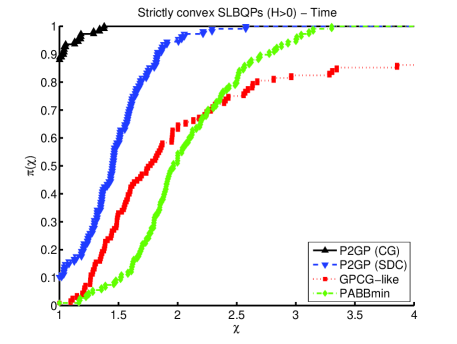
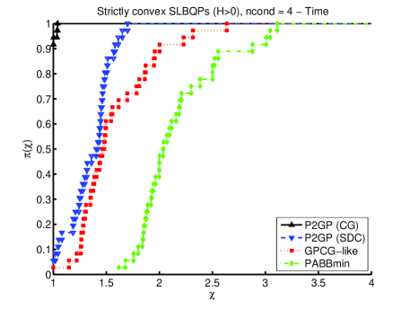
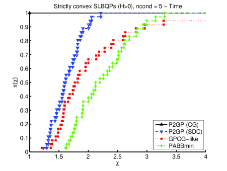
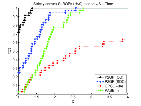
Fig. 1: Performance profiles of P2GP with CG and SDC, PABB_min, and GPCG-like on strictly-convex SLBQPs with nondegenerate solutions: execution times for all the problems (top left), for $\kappa(H)=10^{4}$ (top right), for $\kappa(H)=10^{5}$ (bottom left), and for $\kappa(H)=10^{6}$ (bottom right).

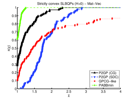
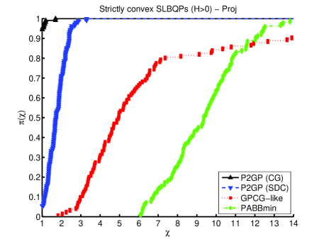
Fig. 2: Performance profiles of P2GP with CG and SDC, PABB_min, and GPCG-like on strictly convex SLBQPs with nondegenerate solutions: number of matrix-vector products (left) and projections (right).

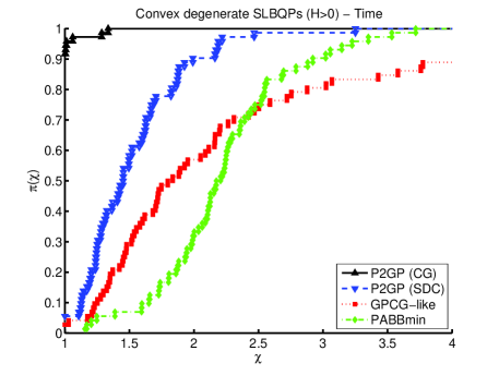
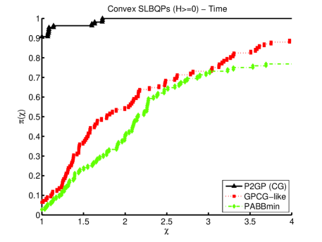
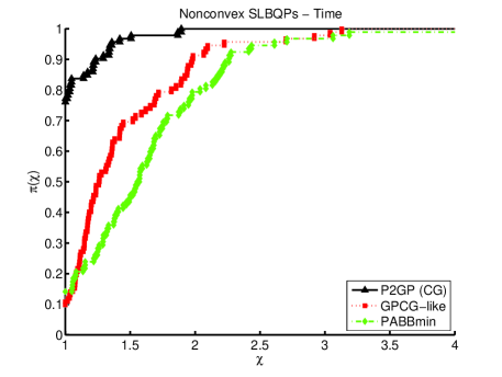
Fig. 3: Performance profiles (execution times) of P2GP with CG and SDC, PABB_min, and GPCG-like on strictly convex SLBQPs with degenerate solutions (top), convex SLBQPs (bottom left), nonconvex SLBQPs (bottom right).

Figure 1 shows the performance profiles, $\pi(\chi)$, of the three methods on the set of strictly convex SLBQPs with nondegenerate solutions, using the execution time as performance metric. The profiles corresponding to all the problems and to those with $\kappa(H)=10^{4}$, $\kappa(H)=10^{5}$, and $\kappa(H)=10^{6}$ are reported. We see that the version of P2GP using CG in the minimization phase has by far the best performance. P2GP with SDC is faster than the PABB_min and GPCG-like methods too. GPCG-like appears very sensitive to the condition number of the Hessian matrix: its performance deteriorates as $\kappa(H)$ increases and the method becomes less effective than PABB_min when $\kappa(H)=10^{6}$. This shows that the criterion used to terminate the minimization phase is more effective than the criterion based on the bindingness of the active variables, especially as $\kappa(H)$ increases. We also report that the GPCG-like method has 6 failures over 36 runs for the problems with $\kappa(H)=10^{6}$.

For the previous problems, the performance profiles concerning the number of matrix-vector products and the number of projections are also shown, in Figure 2. We see that PABB_min performs the smallest number of matrix-vector products, followed by P2GP with GC, and then by GPCG-like and P2GP with SDC. On the other hand, the number of projections computed by P2GP with CG and with SDC is much smaller than for the other methods; as expected, the maximum number of projections is computed by PABB_min. This shows than the performance of the methods cannot be measured only in terms of matrix-vector products; the cost of the projections must also be considered, especially when the structure of the Hessian makes the computational cost of the matrix-vector products lower than $O(n^{2})$. The good behavior of P2GP results from the balance between matrix-vector products and projections.

The performance profiles concerning the execution times on the strictly convex SLBQPs with degenerate solutions, on the convex (but not strictly convex) SLBQPs, and on the nonconvex ones are reported in Figure 3. Of course, the version of P2GP using the SDC solver was not applied to the last two sets of problems. In the case of nonconvex problems, only 85% of the runs were considered, corresponding to the cases where the values of the objective function at the solutions computed by the different methods differ by less than 1%. P2GP with CG is generally the best method, followed by GPCG-like and then by PABB_min. Furthermore, on strictly convex problems with degenerate solutions, P2GP with SDC performs better than GPCG-like and PABB_min. GPCG-like is less robust than the other methods, since it has 4 failures on the degenerate stricltly convex problems and 8 failures on the convex ones. This confirms the effectiveness of the proportionality-based criterion.

For completeness, we also run the experiments on the strictly convex problems with nondegenerate solutions by replacing the line search strategy in PABB_min with a monotone line search along the feasible direction [2, Section 2.3.1], which requires only one projection per GP iteration. We note that this line search does not guarantee in general that the sequence generated by the GP method identifies in a finite number of steps the variables that are active at the solution (see, e.g., [13]). Nevertheless, we made experiments with the line search along the feasible direction, to see if it may lead to any time gain in practice. The results obtained, not reported here for the sake of space, show that the two line searches lead to comparable times when the number of active variables at the solution is small, i.e., naxsol $=0.1$. On the other hand, the execution time with the original line search is slightly smaller when the number of active variables at the solution is larger.

Finally, the performance profiles concerning the execution times taken by the P2GP, PABB_min and GPCG-like methods on the strictly convex BQPs with nondegenerate and degenerate solutions, on the convex (but not strictly convex) BQPs, and on the nonconvex ones are shown in Figure 4. Only 97% of the runs on the nonconvex problems are selected, using the same criterion applied to nonconvex SLBQPs. P2GP with CG is again the most efficient method. The behavior of the methods is similar to that shown on SLBQPs. However, P2GP with SDC and PABB_min have closer behaviors, according to the smaller time required by projections onto boxes, which leads to a reduction of the execution time of PABB_min. GPCG-like has again some failures: 6 on the strictly convex problems with nondegenerate solutions, 5 on the ones with degenerate solutions, and 9 on the convex (but not strictly convex) problems.

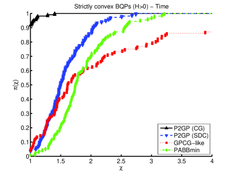
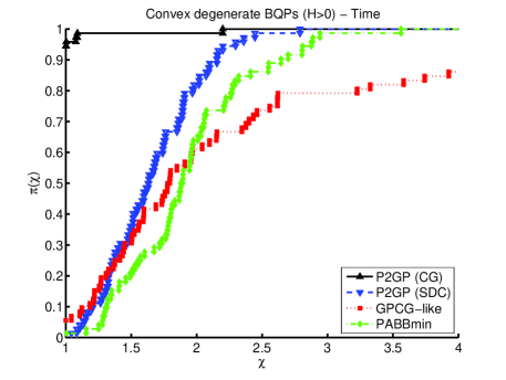
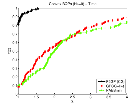
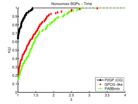
Fig. 4: Performance profiles (execution times) of P2GP with CG and SDC, PABB_min, and GPCG-like on strictly convex BQPs with nondegenerate solutions (top left), strictly convex BQPs with degenerate solutions (top right), convex BQPs (bottom left), nonconvex BQPs (bottom right).

Now we compare P2GP (using CG) with BLG on the random problems. BLG was run in its full-space mode (default mode), because the form of the Hessian (82) does not allow to take advantage of the subspace mode. The stopping condition (68) was implemented in BLG, and the code was run with the same tolerance and the same maximum numbers of matrix-vector products and projections used for P2GP. Default values were used for the remaining parameters of BLG. Of course, a comparison of the two codes in terms of execution time would be misleading, since BLG is written in C, while P2GP has been implemented in Matlab. Therefore, we consider the matrix-vector products. We do not show a comparison in terms of projections too, because BLG does a projection at each iteration, and this generally results in many more projections than P2GP. Performance profiles are provided in Figure 5. The results concerning all the types of convex problems are shown together, since their profiles are similar. On these problems P2GP appears more efficient than BLG; we also verified that the objective function values at the solutions computed by the two codes agree on at least six significant digits and are smaller for P2GP for 70% of the test cases. Furthermore, in four cases BLG does not satisfy condition (68) within the maximum number of matrix-vector products and projections. The situation is different for the nonconvex problems, where the number of matrix-vector products performed by BLG is smaller. In this case, we verified that BLG also used Frank-Wolfe directions, which were never chosen for the convex problems. This not only reduced the number of matrix-vector products, but often led to smaller objective function values. The values of the objective function at the solutions computed by the two methods differ by less than 1% for only 47% of the test cases, which are the ones considered in the performance profiles on the right of Figure 5. On the other hand, in three cases BLG performs the maximum number of matrix-vector products without achieving the required accuracy.

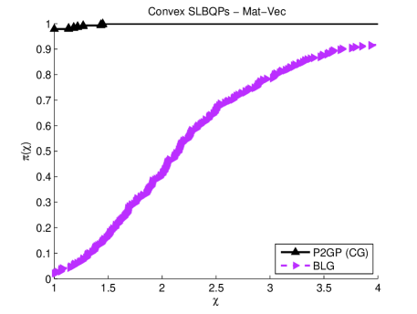
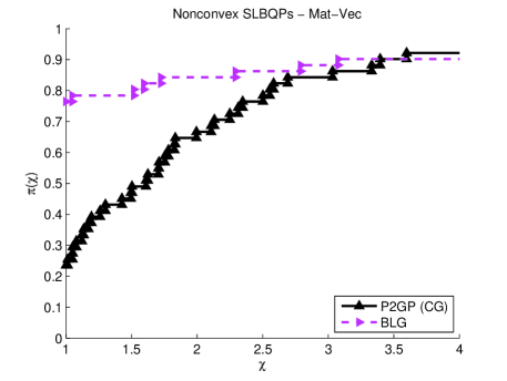
Fig. 5: Performance profiles of P2GP, with CG, and BLG on convex (left) and nonconvex (right) SLBQPs: number of matrix-vector products.

5.4 Results on SVM problems

In order to read the SVM problems, available in the LIBSVM format, BLG was run through the SVMsubspace code, available from http://users.clas.ufl.edu/hager/papers/Software/. Since we were interested in comparing P2GP with the GP implementation provided by BLG, SVMsubspace was modified to have the SVM subspace equal to the entire space, i.e., to apply BLG to the full SVM problem. For completeness we also run SVMsubspace in its subspace mode (see [26]), to see what the performance gain is with this feature. In the following, we refer to the former implementation as BLGfull, and to the latter as SVMsubspace.

Following [26], BLGfull and SVMsubspace were used with their original stopping condition, with tolerance $10^{-3}$. P2GP was terminated when the infinity norm of the projected gradient was smaller then the same tolerance. With these stopping criteria, the two codes returned objective function values agreeing on about six significant digits, with smaller function values generally obtained by P2GP. At most 70000 matrix-vector products and 70000 projections were allowed, but they were never reached.

In Figure 6, left, the performance profiles (in logarithmic scale) concerning the matrix-vector products of P2GP (with CG) and BLGfull are shown. A comparison in terms of projections and execution times is not carried out for the same reasons explained for the random problems. BLGfull appears superior than P2GP; on the other hand, we verified that the number of projections performed by BLG is by far greater than that of P2GP for eight out of ten problems. However, it must be noted that SVMsubspace is much faster than BLGfull, as shown by the performance profiles concerning their execution times (see Figure 6, right). This confirms the great advantage of performing reduced-size matrix-vector products in solving the subspace problems for this class of test cases.

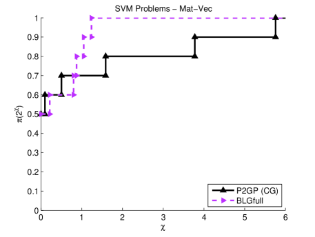
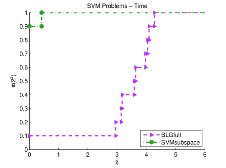
Fig. 6: Performance profiles on SVM test problems: number of matrix-vector of P2GP, with CG, and BLG (left), and execution times of BLG and SVMsubspace (right).

6 Concluding remarks

We presented P2GP, a new method for SLBQPs which has its roots in the GPCG method. The most distinguishing feature of P2GP with respect to GPCG stands in the criterion used to stop the minimization phase. This is a critical issue, since requiring high accuracy in this phase can be a useless and time-consuming task when the face where a solution lies is far from being identified.

Our numerical tests show a strong improvement of the computational performance when the proportionality criterion is used to control the termination of the minimization phase. In particular, the comparison of P2GP with an extension of GPCG to SLBQPs shows the clear superiority of P2GP and its smaller sensitivity to the Hessian condition number. Thus, proportionality allows to handle the minimization phase in a more clever way. The numerical results also show that P2GP requires much fewer projections than efficient GP methods like PABB_min and the one implemented in BLG. This leads to a significant time saving, especially when the Hessian matrix is sparse or has a structure that allows the computation of the matrix-vector product with a computational cost smaller than $O(n^{2})$, where $n$ is the size of the problem. From the theoretical point of view, a nice consequence of using the proportionality criterion is that finite convergence for strictly convex problems can be proved even in case of degeneracy at the solution.

An interesting feature of P2GP is that it provides a general framework, allowing different steplength rules in the GP steps, and different methods in the minimization phase. The encouraging theoretical and computational results suggest that this framework deserves to be further investigated, and possibly extended to more general problems. For example, it would be interesting to extend P2GP to general differentiable objective functions or to problems with bounds and a few linear constraints.

The Matlab code implementing P2GP used in the experiments is available from https://github.com/diserafi/P2GP. It includes the test problem generator described in Section 5.1.

Acknowledgments. We wish to thank William Hager for helpful discussions about the use of the BLG code and for insightful comments on our manuscript. We also express our thanks to the anonymous referees for their useful remarks and suggestions, which allowed us to improve the quality of this work.

References

• [1] S. Amaral, D. L. Allaire, and K. Willcox, Optimal $L_{2}$-norm empirical importance weights for the change of probability measure, Statistics and Computing, 27 (2017), pp. 625–643.
• [2] D. P. Bertsekas, Nonlinear Programming, Athena Scientific, Belmont, MA, USA, 1999.
• [3] R. H. Bielschowsky, A. Friedlander, F. A. M. Gomes, and J. M. Martínez, An adaptive algorithm for bound constrained quadratic minimization, Investigacion Operativa, 7 (1997), pp. 67–102.
• [4] E. G. Birgin, J. M. Martínez, and M. Raydan, Nonmonotone spectral projected gradient methods on convex sets, SIAM Journal on Optimization, 10 (2000), pp. 1196–1211.
• [5] Å. Björck, Numerical methods for least squares problems, SIAM, Philadelphia, PA, USA, 1996.
• [6] S. Bonettini, R. Zanella, and L. Zanni, A scaled gradient projection method for constrained image deblurring, Inverse Problems, 25 (2009), p. 015002.
• [7] P. H. Calamai and J. J. Moré, Projected gradient methods for linearly constrained problems, Mathematical Programming, 39 (1987), pp. 93–116.
• [8] P. H. Calamai and J. J. Moré, Quasi-Newton updates with bounds, SIAM Journal on Numerical Analysis, 24 (1987), pp. 1434–1441.
• [9] L. Condat, Fast projection onto the simplex and the l1 ball, Mathematical Programming, 158 (2016), pp. 575–585.
• [10] F. E. Curtis and W. Guo, Handling nonpositive curvature in a limited memory steepest descent method, IMA Journal of Numerical Analysis, 36 (2016), pp. 717–742.
• [11] Y.-H. Dai and R. Fletcher, Projected Barzilai-Borwein methods for large-scale box-constrained quadratic programming, Numerische Mathematik, 100 (2005), pp. 21–47.
• [12]  , New algorithms for singly linearly constrained quadratic programs subject to lower and upper bounds, Mathematical Programming (Series A), 106 (2006), pp. 403–421.
• [13] P. L. De Angelis and G. Toraldo, On the identification property of a projected gradient method, SIAM Journal on Numerical Analysis, 30 (1993), pp. 1483–1497.
• [14] R. De Asmundis, D. di Serafino, W. W. Hager, G. Toraldo, and H. Zhang, An efficient gradient method using the Yuan steplength, Computational Optimization and Applications, 59 (2014), pp. 541–563.
• [15] R. De Asmundis, D. di Serafino, and G. Landi, On the regularizing behavior of the SDA and SDC gradient methods in the solution of linear ill-posed problems, Journal of Computational and Applied Mathematics, 302 (2016), pp. 81 – 93.
• [16] R. De Asmundis, D. di Serafino, F. Riccio, and G. Toraldo, On spectral properties of steepest descent methods, IMA Journal of Numerical Analysis, 33 (2013), pp. 1416–1435.
• [17] D. di Serafino, V. Ruggiero, G. Toraldo, and L. Zanni, A note on spectral properties of some gradient methods, in Numerical Computations: Theory and Algorithms (NUMTA-2016), vol. 1776 of AIP Conference Proceedings, 2016, p. 040003.
• [18]  , On the steplength selection in gradient methods for unconstrained optimization, Applied Mathematics and Computation, 318 (2018), pp. 176–195.
• [19] E. D. Dolan and J. J. Moré, Benchmarking optimization software with performance profiles, Mathematical Programming, Series B, 91 (2002), pp. 201–213.
• [20] Z. Dostál, Box constrained quadratic programming with proportioning and projections, SIAM Journal on Optimization, 7 (1997), pp. 871–887.
• [21] Z. Dostál and L. Pospíšil, Minimizing quadratic functions with semidefinite Hessian subject to bound constraints, Computers and Mathematics with Applications, 70 (2015), pp. 2014–2028.
• [22] Z. Dostál and J. Schöberl, Minimizing quadratic functions subject to bound constraints with the rate of convergence and finite termination, Computational Optimization and Applications, 30 (2005), pp. 23–43.
• [23] G. Frassoldati, L. Zanni, and G. Zanghirati, New adaptive stepsize selections in gradient methods, Journal of Industrial and Management Optimization, 4 (2008), pp. 299–312.
• [24] A. Friedlander and J. M. Martínez, On the numerical solution of bound constrained optimization problems, RAIRO - Operations Research, 23 (1989), pp. 319–341.
• [25]  , On the maximization of a concave quadratic function with box constraints, SIAM Journal on Optimization, 4 (1994), pp. 177–192.
• [26] M. D. Gonzalez-Lima, W. W. Hager, and H. Zhang, An affine-scaling interior-point method for continuous knapsack constraints with application to support vector machines, SIAM Journal on Scientific Computing, 21 (2011), pp. 361–390.
• [27] W. W. Hager and H. Zhang, A new active set algorithm for box constrained optimization, SIAM Journal on Optimization, 17 (2006), pp. 526–557.
• [28]  , An active set algorithm for nonlinear optimization with polyhedral constraints, Science China Mathematics, 59 (2016), pp. 1525–1542.
• [29] P. Kamesam and R. Meyer, Multipoint methods for separable nonlinear networks, Springer, 1984.
• [30] H. Mohy-ud-Din and D. P. Robinson, A solver for nonconvex bound-constrained quadratic optimization, SIAM Journal on Optimization, 25 (2015), pp. 2385–2407.
• [31] J. Moré and G. Toraldo, Algorithms for bound constrained quadratic programming problems, Numerische Mathematik, 55 (1989), pp. 377–400.
• [32] J. J. Moré and G. Toraldo, On the solution of large quadratic programming problems with bound constraints, SIAM Journal on Optimization, 1 (1991), pp. 93–113.
• [33] P. M. Pardalos and J. B. Rosen, Constrained global optimization: algorithms and applications, Springer-Verlag, New York, NY, USA, 1987.
• [34] B. N. Parlett, The Symmetric Eigenvalue Problem, SIAM, Philadelphia, PA, USA, 1998.
• [35] T. Serafini, G. Zanghirati, and L. Zanni, Gradient projection methods for quadratic programs and applications in training support vector machines, Optimization Methods and Software, 20 (2005), pp. 353–378.
• [36] V. N. Vapnik and S. Kotz, Estimation of dependences based on empirical data, vol. 40, Springer-Verlag, New York, NY, USA, 1982.
• [37] Y. Yuan, A new stepsize for the steepest descent method, Journal of Computational Mathematics, 24 (2006), pp. 149–156.