An optimal transportation approach for assessing almost stochastic order.

Abstract

When stochastic dominance $F\leq_{st}G$ does not hold, we can improve agreement to stochastic order by suitably trimming both distributions. In this work we consider the $L_{2}-$Wasserstein distance, $\mathcal{W}_{2}$, to stochastic order of these trimmed versions. Our characterization for that distance naturally leads to consider a $\mathcal{W}_{2}$-based index of disagreement with stochastic order, $\varepsilon_{\mathcal{W}_{2}}(F,G)$. We provide asymptotic results allowing to test $H_{0}:\varepsilon_{\mathcal{W}_{2}}(F,G)\geq\varepsilon_{0}$ vs $H_{a}:\varepsilon_{\mathcal{W}_{2}}(F,G)<\varepsilon_{0}$, that, under rejection, would give statistical guarantee of almost stochastic dominance. We include a simulation study showing a good performance of the index under the normal model.

1 Introduction

Let $P,Q$ be probability distributions on the real line with distribution functions (d.f.’s in the sequel) $F,G$, respectively. Stochastic dominance of $Q$ over $P$, denoted $P\leq_{st}Q,$ is defined in terms of the d.f.’s by $F(x)\geq G(x)$ for every $x\in\mbox{$\mathbb{R}$}$ (throughout we will also use the alternative notation $F\leq_{st}G$). The meaning of this relation is that random outcomes produced by the second law tend to be larger than those produce by the first one. We gain a better understanding of this stochastic order by considering a quantile representation. For a d.f. $F$, the quantile function associated to $F$, that we will denote by $F^{-1}$, is defined by

$$F^{-1}(t)=\inf\{x:t\leq F(x)\},\ t\in(0,1).$$

The following well-known statements (see e.g. [15]) are equivalent to $F\leq_{st}G$:

• There exist random variables $X,Y$ defined on some probability space $(\Omega,\sigma,\mu)$, with respective laws $P$ and $Q$ ($\mathcal{L}(X)=P,\mathcal{L}(Y)=Q$), satisfying $\mu(X\leq Y)=1$.

• $F^{-1}(t)\leq G^{-1}(t)$ for every $t\in(0,1)$.

Quantile functions (also called ‘monotone rearrangements’ in other contexts) are characterized by $F^{-1}(t)\leq x$ if and only if $t\leq F(x)$. Therefore it is straightforward that, when considered as random variables defined on the unit interval with the Lebesgue measure $((0,1),\beta_{(0,1)},\ell)$, they satisfy $\mathcal{L}(F^{-1})=P,\mathcal{L}(G^{-1})=Q$. This representation shows that a) and b) are equivalent and, more importantly in the present setting, allows us to relate characteristics and measure agreement or disagreements with the stochastic order.

From the previous considerations it becomes clear that guaranteeing stochastic dominance, $F\leq_{st}G$, should be the goal when comparing treatments or production schemes. However, the rejection of $F\nleq_{st}G,$ on the basis of two data samples is an ill posed statistical problem: As showed in [8] and noted in [17], [13], or [5], the ‘non-data test’, namely the test which rejects with probability $\alpha$, regardless the data, is uniformly most powerful for testing the nonparametric hypotheses $H_{0}:F\nleq_{st}G$ vs $H_{a}:F\leq_{st}G$. This fact motivates recent research looking for suitable indices measuring ‘almost’ or ‘approximate’ versions of stochastic dominance. Here, suitability of an index must be understood in terms of computability and interpretability, but also in terms of statistical performance. Usually, as already suggested in a general context in [14], such measures of nearness involve the use of some kind of distance to the null. This will also be the approach here, with the choice of the $L_{2}$-Wasserstein distance between probabilities. For $P,Q$ in the set $\mathcal{F}_{2}(\mbox{$\mathbb{R}^{d}$})$ of Borel probabilities on $\mathbb{R}^{d}$ with finite second order moments, this distance is defined as

$$\mathcal{W}_{2}(P,Q):=\min\left\{\int\|x-y\|^{2}d\nu(x,y),\nu\in\mathcal{F}_{2}(\mbox{$\mathbb{R}^{d}$}\times\mbox{$\mathbb{R}^{d}$})\mbox{ with marginals }P,Q\right\}^{1/2}.$$

In the univariate case, $\mathcal{W}_{2}$ equals the $L_{2}$-distance between quantile functions, namely,

$$\mathcal{W}_{2}(P,Q)=\left(\int_{0}^{1}|F^{-1}(t)-G^{-1}(t)|^{2}dt\right)^{1/2}.$$ (1)

Statistical applications based on optimal transportation, and particularly on the $L_{2}$ version, are receiving considerable attention in recent times (see e.g. [9], [10], [11], [18] or [6]). We should mention here our papers [2] and [3], dealing with similarity of distributions (as a relaxation of homogeneity) through this distance, and also [5] (and [4]) which introduced an index of disagreement from stochastic dominance based on the idea of similarity. The key to this index is the existence, for a given (small enough) $\pi,$ of mixture decompositions

$$\left\{\begin{matrix}F&=&(1-\pi)\tilde{F}+\pi H_{F}\\ &&\\ G&=&(1-\pi)\tilde{G}+\pi H_{G},\end{matrix}\right.\quad\mbox{ for some d.f.'s }\tilde{F},H_{F},\tilde{G},H_{G}\mbox{ such that }\tilde{F}\leq_{st}\tilde{G}.$$ (2)

If model (2) holds then it means that stochastic order holds after removing contaminating $\pi$-fractions from each population. The minimum $\pi$ compatible with (2), denoted by $\pi(F,G)$, can then be taken as a measure of deviation from stochastic order, see [5] for details. We would like to emphasize here that the analysis in [5] is based on the connection between contamination models and trimmed probabilities. We recall that an $\alpha$-trimming of a probability, $P$, is any other probability, say $\tilde{P}$, such that

$$\tilde{P}(A)=\int_{A}\tau dP\quad\mbox{ for everys event }A$$

for some function $\tau$ taking values in $[0,\frac{1}{1-\alpha}]$. Like the trimming methods, commonly used in Robust Statistics, consisting of removing disturbing observations, the function $\tau$ allows to discard or downplay the influence of some regions on the sample space. On the real line, writing $\mathcal{R}_{\alpha}(F)$ for the set of trimmings of $F$, it turns out (see [5]) that

$$F=(1-\alpha)\tilde{F}+\alpha H_{F}\mbox{ for some d.f.'s }\tilde{F},H_{F}\mbox{ if and only if }\tilde{F}\in\mathcal{R}_{\alpha}(F).$$ (3)

The contaminated stochastic order model (2) can also be recast in terms of trimmings. If we denote

$$\mathcal{F}_{st}:=\{(H_{1},H_{2})\in\mathcal{F}_{2}\times\mathcal{F}_{2}:\quad H_{1}\leq_{st}H_{2}\},$$

then, for $F,G\in\mathcal{F}_{2}$, (2) holds if and only if

$$(\mathcal{R}_{\pi}(F)\times\mathcal{R}_{\pi}(G))\cap\mathcal{F}_{st}\neq\emptyset$$ (4)

or, equivalently (this follows from compactness of $\mathcal{R}_{\pi}(F)\times\mathcal{R}_{\pi}(G)$ with respect to $d_{2}$; we omit details), if and only if

$$d_{2}(\mathcal{R}_{\pi}(F)\times\mathcal{R}_{\pi}(G),\mathcal{F}_{st})=0,$$ (5)

where $d_{2}$ denotes the metric on the set $\mathcal{F}_{2}\times\mathcal{F}_{2}$ given by

$$d_{2}((F_{1},F_{2}),(G_{1},G_{2}))=\sqrt{\mathcal{W}_{2}^{2}(F_{1},G_{1})+\mathcal{W}_{2}^{2}(F_{2},G_{2})}$$

and, for $A,B\subset\mathcal{F}_{2}\times\mathcal{F}_{2}$, $d_{2}(A,B)=\inf_{a\in A,b\in B}d_{2}(a,b)$.

For fixed $\pi$, $d_{2}(\mathcal{R}_{\pi}(F)\times\mathcal{R}_{\pi}(G),\mathcal{F}_{st})$ can be used as a measure of deviation from the contaminated stochastic order model (2). In this work we obtain a simple explicit characterization of this measure (see Theorem 2.3 below) that could be used for statistical purposes. Later, we use this characterization to introduce a new index, $\varepsilon_{\mathcal{W}_{2}}$, see (8), to evaluate disagreement with respect to the (non-contaminated) stochastic order. We also provide asymptotic theory (Theorem 2.4) about the behavior of this index, that allows addressing the goal of statistical assessment of $\varepsilon_{\mathcal{W}_{2}}$-almost stochastic dominance. This index has some similarity with that proposed in [17] for which, in contrast, asymptotics are not available.

The remaining sections of this work are organized as follows. Section 2 presents the announced results, introduces the new index $\varepsilon_{\mathcal{W}_{2}}$ and discusses its application in the statistical assessment of almost stochastic order. This includes an illustration of the meaning of the index in the case of normal distributions and a small simulation study. Finally, the more technical proof of Theorem 2.4 is given in an Appendix.

2 Main results

A fortunate fact that eases the use of trimming in the stochastic dominance setting is that the set $\mathcal{R}_{\alpha}(F)$ has a minimum and a maximum for the stochastic order. Moreover both can be easily characterized as follows (see Proposition 2.3 in [5]).

Proposition 2.1

Consider a distribution function $F$ and $\pi\in[0,1)$. Define the d.f.’s

$$F^{\pi}(x)=\max({\textstyle\frac{1}{1-\pi}}(F(x)-\pi),0)\quad\mbox{and}\quad F_{\pi}(x)=\min({\textstyle\frac{1}{1-\pi}}F(x),1).$$

Then $F^{\pi},F_{\pi}\in\mathcal{R}_{\pi}(F)$ and any other $\tilde{F}\in\mathcal{R}_{\pi}(F)$ satisfies $F_{\pi}\leq_{st}\tilde{F}\leq_{st}F^{\pi}$.

Recalling the characterization of the stochastic order in terms of quantile functions, a simple computation shows that the associated quantile functions are

$$(F_{\pi})^{-1}(t)=F^{-1}((1-\pi)t),\quad(F^{\pi})^{-1}(t)=F^{-1}(\pi+(1-\pi)t),\quad 0<t<1,$$ (6)

so we can restate this proposition in the following new way.

Proposition 2.2

If $\tilde{F}\in\mathcal{R}_{\pi}(F)$, then its quantile function satisfies

$$F^{-1}((1-\pi)t)\leq\tilde{F}^{-1}(t)\leq F^{-1}(\pi+(1-\pi)t),\quad 0<t<1.$$ (7)

We can use equation (7) for proving our next result, the announced characterization for $d_{2}(\mathcal{R}_{\pi}(F)\times\mathcal{R}_{\pi}(G),\mathcal{F}_{st})$, a quantity that measures deviation from the contaminated stochastic order model (2). We keep the notation in (6) and define

$$(L_{\pi})^{-1}(t)=\left\{\begin{matrix}(F_{\pi})^{-1}(t)&\mbox{ if }(F_{\pi})^{-1}(t)\leq(G^{\pi})^{-1}(t)\\ \frac{1}{2}((F_{\pi})^{-1}(t)+(G^{\pi})^{-1}(t))&\mbox{ if }(F_{\pi})^{-1}(t)>(G^{\pi})^{-1}(t)\end{matrix}\right.$$

$$(U_{\pi})^{-1}(t)=\left\{\begin{matrix}(G^{\pi})^{-1}(t)&\mbox{ if }(F_{\pi})^{-1}(t)\leq(G^{\pi})^{-1}(t)\\ \frac{1}{2}((F_{\pi})^{-1}(t)+(G^{\pi})^{-1}(t))&\mbox{ if }(F_{\pi})^{-1}(t)>(G^{\pi})^{-1}(t).\end{matrix}\right.$$

Theorem 2.3

With the above notation, if $F$ and $G$ are distribution functions with finite second moment the $L_{\pi}^{-1}$, $U_{\pi}^{-1}$ are the quantile functions of a pair $(L_{\pi},U_{\pi})\in\mathcal{F}_{st}$. Furthermore, if we denote $x_{+}=\max(x,0)$,

$$d_{2}(\mathcal{R}_{\pi}(F)\times\mathcal{R}_{\pi}(G),\mathcal{F}_{st}) = d_{2}((F_{\pi},G^{\pi}),(L_{\pi},U_{\pi}))$$

$$= \sqrt{\frac{1}{2}\int_{0}^{1}(F^{-1}((1-\pi)t)-G^{-1}(\pi+(1-\pi)t))_{+}^{2}dt}.$$

Proof. To see that $(L_{\pi})^{-1}$ is a quantile function we note that

$$(L_{\pi})^{-1}(t)=\min((F_{\pi})^{-1}(t),{\textstyle\frac{1}{2}}((F_{\pi})^{-1}(t)+(G^{\pi})^{-1}(t))).$$

This shows that $(L_{\pi})^{-1}$ is nondecreasing and left continuous, hence a quantile function. That $L_{\pi}$ has finite second moment follows from the elementary bounds

$$-(|(F_{\pi})^{-1}(t)|+|(G^{\pi})^{-1}(t)|)\leq(L_{\pi})^{-1}(t)\leq(F_{\pi})^{-1}(t).$$

A similar argument works for $U_{\pi}$. Obviously $L_{\pi}\leq_{st}U_{\pi}$ and, therefore, $(L_{\pi},U_{\pi})\in\mathcal{F}_{st}$. Now, for any $(U_{1},U_{2})\in\mathcal{R}_{\pi}(F)\times\mathcal{R}_{\pi}(G)$ and $(V_{1},V_{2})\in\mathcal{F}_{st}$ we have $U_{1}^{-1}(t)\geq(F_{\pi})^{-1}(t)$, $U_{2}^{-1}(t)\leq(G^{\pi})^{-1}(t)$, $V_{1}^{-1}(t)\leq V_{2}^{-1}(t)$. We define $A_{\pi}:=\{t\in(0,1):\,(F_{\pi})^{-1}(t)>(G^{\pi})^{-1}(t)\}$. Then

$$d_{2}((U_{1},U_{2}),(V_{1},V_{2})) = \int_{0}^{1}((U_{1}^{-1}(t)-V_{1}^{-1}(t))^{2}+(U_{2}^{-1}(t)-V_{2}^{-1}(t))^{2})dt$$

$$\geq \int_{A_{\pi}}((U_{1}^{-1}(t)-V_{1}^{-1}(t))^{2}+(U_{2}^{-1}(t)-V_{2}^{-1}(t))^{2})dt$$

$$\geq \int_{A_{\pi}}(((F_{\pi})^{-1}(t)-(L_{\pi})^{-1}(t))^{2}+((G^{\pi})^{-1}(t)-(U_{\pi})^{-1}(t))^{2})dt$$

$$= \int_{0}^{1}(((F_{\pi})^{-1}(t)-(L_{\pi})^{-1}(t))^{2}+((G^{\pi})^{-1}(t)-(U_{\pi})^{-1}(t))^{2})dt$$

$$= d_{2}((F_{\pi},G^{\pi}),(L_{\pi},U_{\pi})),$$

where the last lower bound is just the trivial fact that if $f>g$, then the minimum value $\min_{a,b,c,d}(a-b)^{2}+(c-d)^{2}$, for $a\geq f,c\leq g,b\leq d$ is just attained at $a=f$, $c=g$, $b=d=\frac{f+g}{2}$. To complete the proof we note that

$$d_{2}((F_{\pi},G^{\pi}),(L_{\pi},U_{\pi})) = \frac{1}{2}\int_{A_{\pi}}((F_{\pi})^{-1}(t)-(G^{\pi})^{-1}(t))^{2}dt$$

$$= \frac{1}{2}\int_{0}^{1}(F^{-1}((1-\pi)t)-G^{-1}(\pi+(1-\pi)t))_{+}^{2}dt$$

$\bullet$

Particularizing for $\pi=0$, Theorem 2.3 shows that the distance $d_{2}$ between the pair $(F,G)$ and the set $\mathcal{F}_{st}$ is attained at the pair $(L_{0},U_{0})\in\mathcal{F}_{st}$ associated to the quantile functions $L_{0}^{-1}=\inf\{F^{-1},(F^{-1}+G^{-1})/2\}$ and $U_{0}^{-1}=\sup\{G^{-1},(F^{-1}+G^{-1})/2\}$. Moreover, $d_{2}^{2}((F,G),\mathcal{F}_{st})=\frac{1}{2}\int_{0}^{1}(F^{-1}(t)-G^{-1}(t))_{+}^{2}dt$. Avoiding the factor $1/2$, this is just the part of $\mathcal{W}_{2}^{2}(F,G)$ due to the violation of stochastic dominance. Therefore, for distinct d.f.’s $F,G$, according to the notation $A_{0}=\{t\in(0,1):F^{-1}(t)>G^{-1}(t)\}$, the quotient

$$\varepsilon_{\mathcal{W}_{2}}(F,G):=\frac{\int_{A_{0}}(F^{-1}(t)-G^{-1}(t))^{2}dt}{\mathcal{W}_{2}^{2}(F,G)}$$ (8)

can be considered as a normalized index of such violation. It satisfies $0\leq\varepsilon_{\mathcal{W}_{2}}(F,G)\leq 1,$ with the extreme values 0 and 1 corresponding, respectively, to perfect stochastic dominance of $G$ over $F$ and vice-versa. We notice that [17], following a very different motivation, introduced a related index consisting in the quotient ${\int_{F<G}(G(x)-F(x))dx}/{\|F-G\|_{1}},$ where $\|-\|_{1}$ is the $L_{1}-$ norm with respect to the Lebesgue measure on the line.

The index $\varepsilon_{\mathcal{W}_{2}}(F,G)$ can be estimated by its sample counterpart $\varepsilon_{\mathcal{W}_{2}}(F_{n},G_{m})$, when $F_{n}$ and $G_{m}$ are the sample d.f.’s associated to independent samples respectively obtained from $F$ and $G$. The following theorem gives the mathematical background for such task.

Theorem 2.4

Let $F,G$ be distinct d.f.’s in $\mathcal{F}_{2}$ and assume $n,m\to\infty$ with $\frac{n}{n+m}\to\lambda\in(0,1)$. If $F_{n}$ and $G_{m}$ are the sample d.f.’s based on independent samples of $F$ and $G$, then $\varepsilon_{\mathcal{W}_{2}}(F_{n},G_{m})\to\varepsilon_{\mathcal{W}_{2}}(F,G)$ a.s.. If, additionally, $F$ and $G$ have bounded convex supports, then

$$\sqrt{\frac{mn}{m+n}}\left(\varepsilon_{\mathcal{W}_{2}}(F_{n},G_{m})-\varepsilon_{\mathcal{W}_{2}}(F,G)\right)\rightarrow_{w}N(0,\sigma^{2}_{\lambda}(F,G)),$$ (9)

where

$$\sigma^{2}_{\lambda}(F,G)=\frac{1}{\mathcal{W}_{2}^{8}(F,G)}[(1-\lambda)\mbox{\em Var}(u_{-}(X))+\lambda\mbox{\em Var}(u_{+}(Y))],$$

$u_{+}(x)=\int_{0}^{x}2(s-G^{-1}(F(s)))_{+}ds$, $u_{-}(x)=\int_{0}^{x}2(s-G^{-1}(F(s)))_{-}ds$ and $X$ and $Y$ are independent r.v.’s with d.f.’s $F$ and $G$, respectively.

A critical analysis of the problem of assessing improvement in a treatment comparison setup from the perspective of stochastic dominance is given in [7]. It is argued there that under, say, normality assumptions, improvement with the new treatment is often assessed through a one sided test for the mean, while the really interesting test would be that of $F\nleq_{st}G$ vs $F\leq_{st}G$. Since, as argued in the Introduction, this is not a feasible statistical task, we emphasized there on the alternative, feasible goal of testing that slightly relaxed versions of stochastic dominance hold. In the present setting, such a strategy leads to consider the problem of testing, at a given confidence level, $H_{0}:\varepsilon_{\mathcal{W}_{2}}(F,G)\geq\varepsilon_{0}$ vs $H_{a}:\varepsilon_{\mathcal{W}_{2}}(F,G)<\varepsilon_{0}$, where $\varepsilon_{0}$ is a small enough prefixed amount of disagreement with the stochastic order.

Following the scheme in [5] and [7], from the asymptotic normality obtained in Theorem 2.4 we propose to reject $H_{0}$ if

$$\textstyle{\sqrt{\frac{nm}{n+m}}(\varepsilon_{\mathcal{W}_{2}}(F_{n},G_{m})-\varepsilon_{0})<\hat{\sigma}_{n,m}\Phi^{-1}(\alpha)},$$ (10)

where $\hat{\sigma}_{n,m}$ is an estimator of $\sigma_{\lambda}(F,G)$ (for example a bootstrap estimator). This rejection rule provides a consistent test of asymptotic level $\alpha$. Also,

$$\hat{U}:=\varepsilon_{\mathcal{W}_{2}}(F_{n},G_{m})-\textstyle\sqrt{\frac{n+m}{nm}}\hat{\sigma}_{n,m}\Phi^{-1}(\alpha)$$ (11)

provides an upper confidence bound for $\varepsilon_{\mathcal{W}_{2}}(F,G)$ with asymptotic level $1-\alpha$.

Let us take now a closer look at the $\varepsilon_{\mathcal{W}_{2}}$ index for distributions in a location-scale family. For simplicity, we focus on normal laws. It is an elementary fact that $\varepsilon_{\mathcal{W}_{2}}$ is invariant to changes in location and scale and we can, consequently, resctrict ourselves to the analysis of Therefore we can obtain the values of $\varepsilon_{\mathcal{W}_{2}}(N(0,1),N(\mu,\sigma^{2}))$, $\mu\in\mathbb{R},\sigma>0$. 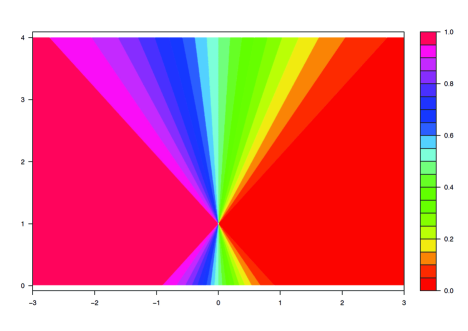Moreover, it is easy to see that $\varepsilon_{\mathcal{W}_{2}}$ is constant when $(\mu,\sigma)$ moves along directed rays from $(0,1)$. This fact is showed in figure 1. We see that $\mu>0$ corresponds to $\varepsilon_{\mathcal{W}_{2}}(N(0,1),N(\mu,\sigma^{2}))<\frac{1}{2}$, with $\varepsilon_{\mathcal{W}_{2}}(N(0,1),N(\mu,1))=0$, but the index can be made arbitrarily close to $\frac{1}{2}$ by taking $\sigma$ large enough.

Finally, we present in Table 1 some simulations showing the performance of the proposed nonparametric procedure. We see the observed rejection rates for the test (10). In our simulations we have taken $F=N(0,1)$ and $G=N(\mu,\sigma^{2})$ for several choices of $\mu,\sigma$. We show also the rejection rates based on a natural competitor, the parametric maximum likelihood estimator $\hat{\varepsilon}_{\mathcal{W}_{2}}:=\varepsilon_{\mathcal{W}_{2}}(F_{N(\bar{X}_{n},S_{X}^{2})},F_{N(\bar{Y}_{m},S_{Y}^{2})})$. This estimator is, of course, highly nonrobust and useless in practice without the a priori knowledge that $F$ and $G$ are normal, but we use it here as a benchmark. We see a reasonable amount of agreement of the rejection frequencies to the nominal level of the test, even if it is slightly liberal for $\sigma$ close to one and small $\varepsilon_{0}$, but the nonparamentric procedure does not perform worse than the parametric benchmark. We also see that it is possible to get statistical evidence that almost stochastic order does hold. For instance, for $\mu=.697$, $\sigma=1.5$ (true $\varepsilon_{\mathcal{W}_{2}}=0.01$) sizes $n=m=1000$ suffice to conclude that $\varepsilon_{\mathcal{W}_{2}}<0.05$ with probability close to $0.93$.

Figure 1: Contour-plot of $\varepsilon_{\mathcal{W}_{2}}(N(0,1),N(\mu,\sigma^{2}))$ as in (8) for different values of $\mu$ (X-axis) and $\sigma$ (Y-axis)

Table 1: Rejection rates for $\varepsilon_{\mathcal{W}_{2}}(N(0,1),N(\mu,\sigma^{2}))\geq\varepsilon_{0}$ at level $\alpha=.05$ along 1,000 simulations. Upper (resp. lower) rows show results for nonparametric (resp. parametric) comparisons. For each $\sigma$, $\mu$ is chosen to make $\varepsilon_{\mathcal{W}_{2}}(N(0,1),N(\mu,\sigma^{2}))=$ 0.01, 0.05 and 0.10 (first, second and third columns, resp.).

		$\sigma=1.1$			$\sigma=1.5$			$\sigma=2$
	Sample	$\mu$			$\mu$			$\mu$
$\varepsilon_{0}$	size	$.139$	$.091$	$.068$	$.697$	$.455$	$.341$	$1.395$	$.909$	$.683$
.01	100	.000	.000	.000	.053	.007	.000	.180	.009	.004
		.000	.000	.000	.062	.006	.000	.112	.003	.000
	1000	.004	.000	.000	.086	.000	.000	.116	.000	.000
		.036	.002	.000	.086	.000	.000	.086	.000	.000
	5000	.014	.000	.000	.084	.000	.000	.077	.000	.000
		.078	.003	.000	.086	.000	.000	.060	.000	.000
.05	100	.013	.004	.004	.321	.060	.019	.677	.138	.028
		.017	.007	.004	.382	.064	.027	.690	.086	.017
	1000	.101	.017	.004	.929	.088	.003	.999	.101	.000
		.219	.041	.015	.982	.087	.002	1.000	.085	.000
	5000	.488	.056	.009	1.000	.067	.000	1.000	.070	.000
		.704	.099	.009	1.000	.069	.000	1.000	.057	.000
.10	100	.034	.017	.006	.608	.210	.092	.930	.402	.148
		.040	.022	.009	.658	.205	.073	.941	.364	.109
	1000	.267	.082	.020	1.000	.545	.076	1.000	.861	.096
		.431	.132	.047	1.000	.642	.076	1.000	.928	.084
	5000	.867	.246	.058	1.000	.970	.056	1.000	1.000	.078
		.960	.356	.087	1.000	.994	.058	1.000	1.000	.069

3 Appendix

We prove here central limit theorems for the index $\varepsilon_{\mathcal{W}_{2}}$ in (8). We will assume that $U_{1},\ldots,U_{n},V_{1},\ldots,V_{m}$ are i.i.d. random variables, uniformly distributed on $(0,1)$. We consider independent samples i.i.d. $X_{1},\ldots,X_{n}$ and $Y_{1},\ldots,Y_{m}$ such that the d.f. of the $X_{i}$ and the $Y_{j}$ are $F$ and $G$, respectively. We note that, without loss of generality, we can assume that the $X_{i}$ and $Y_{j}$ are generated from the $U_{i}$ and the $V_{j}$ through $X_{i}=F^{-1}(U_{i})$, $Y_{j}=G^{-1}(V_{j})$. We write $F_{n}$, $G_{m}$, $H_{n,1}$ and $H_{m,2}$ for the empirical d.f.’s on the $X_{i}$, the $Y_{j}$, $U_{i}$ and the $V_{j}$, respectively. Note that, in particular, $F_{n}^{-1}(t)=F^{-1}(H_{n,1}^{-1}(t))$, $G_{m}^{-1}(t)=G^{-1}(H_{m,2})$. Finally, $\alpha_{n,1}$ and $\alpha_{m,2}$ will denote the empirical processes associated to the $U_{i}$ and the $Y_{j}$, namely, $\alpha_{n,1}(t)=\sqrt{n}(H_{n,1}(t)-t)$, $0\leq t\leq 1$, and similarly for $\alpha_{m,2}$ and we will write $\alpha_{n,1}(h)$ instead of $\int_{0}^{1}h(t)d\alpha_{n,1}(t)$.

We introduce the statistics $S_{n}=\int_{0}^{1}(F_{n}^{-1}-G^{-1})^{2}$, $S_{n}^{+}=\int_{0}^{1}(F_{n}^{-1}-G^{-1})_{+}^{2}$, $S_{n}^{-}=\int_{0}^{1}(F_{n}^{-1}-G^{-1})_{-}^{2}$, and write $S$, $S^{+}$, $S_{-}$ for the corresponding population counterparts. Note that, to ensure that $S$ is finite, $F$ and $G$ should have, at least, finite second moments. However, to simplify the arguments our proof will require bounded supports. We set

$$T_{n}=\sqrt{n}(S_{n}-S),\quad T_{n}^{+}=\sqrt{n}(S^{+}_{n}-S^{+}),\quad T_{n}^{-}=\sqrt{n}(S_{n}^{-}-S^{-}),$$

$c(x)=2x$, $c_{+}(x)=2x_{+}$, $c_{-}(x)=2x_{-}$ and define

$$\textstyle v(t)=\int_{0}^{F^{-1}(t)}c(s-G^{-1}(F(s)))ds$$ (12)

and similarly $v_{+}$ and $v_{-}$ replacing $c$ with $c_{+}$ and $c_{-}$, respectively. Observe that $v=v_{+}-v_{-}$. We this notation we have the following result.

Theorem 3.1

If $F$ and $G$ have bounded support and $G^{-1}$ is continuous on $(0,1)$ then

$$T_{n}=\alpha_{n,1}(v)+o_{P}(1),\quad T^{+}_{n}=\alpha_{n,1}(v_{+})+o_{P}(1),\quad T^{-}_{n}=\alpha_{n,1}(v_{-})+o_{P}(1).$$

Proof. We assume that $|F^{-1}(t)|\leq M$, $|G^{-1}(t)|\leq M$ for all $t\in(0,1)$ and some $M>0$. The continuity and boundedness assumption on $G^{-1}$ allows us to assume that $G^{-1}$ is a continuous function on $[0,1]$, hence, uniformly coutinuous and its modulus of continuity,

$$\textstyle\omega(\delta)=\sup_{|t_{1}-t_{2}|\leq\delta}|G^{-1}(t_{1})-G^{-1}(t_{2})|,$$

satisfies $\omega(\delta)\to 0$ as $\delta\to 0$. It is convenient at this point to note that $T_{n}$ is a function of the $U_{i}$ and also of $F$ and we stress this fact writing $T_{n}(F)$ instead of $T_{n}$ in this proof, and the same for $T_{n}^{+}$ and $T_{n}^{-}$. Similarly, we set $\tilde{T}_{n}(F)=\alpha_{n,1}(v)$, $\tilde{T}_{n}^{+}(F)=\alpha_{n,1}(v_{+})$, $\tilde{T}_{n}^{-}(F)=\alpha_{n,1}(v_{-})$. We claim now that

$$\textstyle E|T_{n}(F)-\tilde{T}_{n}(F)|^{2}\leq 16M^{2}E\Big{(}\|\alpha_{n,1}\|^{2}\omega^{2}\Big{(}\frac{\|\alpha_{n,1}\|}{\sqrt{n}}\Big{)}\Big{)},$$ (13)

where $\|\alpha_{n,1}\|=\sup_{0\leq t\leq 1}|\alpha_{n,1}(t)|$. To check this, let us assume first that $F$ is finitely supported, say on $-M\leq x_{1}<\ldots<x_{k}\leq M$ with $F(x_{j})=s_{j}$, $j=1,\ldots,k$ This means that $F^{-1}(t)=x_{i}$ if $s_{i-1}<t\leq s_{i}$ (we set $s_{0}=0$ for convenience) and we have

$$\textstyle\int_{0}^{1}(F^{-1}-G^{-1})^{2} = \textstyle\sum_{i=1}^{k}\int_{s_{i-1}}^{s_{i}}(x_{i}-G^{-1}(t))^{2}dt=\int_{0}^{1}(x_{k}-G^{-1}(t))^{2}dt$$

$$\textstyle-\sum_{i=1}^{k-1}\int_{0}^{s_{i}}\big{[}(x_{i+1}-G^{-1}(t))^{2}-(x_{i}-G^{-1}(t))^{2}\big{]}dt$$

$$= \textstyle\int_{0}^{1}(x_{k}-G^{-1}(t))^{2}dt-\sum_{i=1}^{k-1}\int_{0}^{s_{i}}\big{[}\int_{x_{i}}^{x_{i+1}}c(s-G^{-1}(t))ds\big{]}dt.$$

A similar expression holds for $\int_{0}^{1}(F_{n}^{-1}-G^{-1})^{2}$ replacing $s_{i}$ with $H_{n,1}(s_{i})$ and we see that

$$\textstyle T_{n}(F)=-\sqrt{n}\sum_{i=1}^{k-1}\int_{s_{i}}^{H_{n,1}(s_{i})}\Big{(}\int_{x_{i}}^{x_{i+1}}c(s-G^{-1}(t))ds\Big{)}dt.$$

We can argue analogously to check that

$$\tilde{T}_{n}(F) = \textstyle-\sum_{i=1}^{k-1}\alpha_{n,1}(s_{i})\Big{(}\int_{x_{i}}^{x_{i+1}}c(s-G^{-1}(s_{i}))ds\Big{)}$$

$$= \textstyle-\sqrt{n}\sum_{i=1}^{k-1}\int_{s_{i}}^{H_{n,1}(s_{i})}\Big{(}\int_{x_{i}}^{x_{i+1}}c(s-G^{-1}(s_{i}))ds\Big{)}dt.$$

Hence, we see that

$$|T_{n}(F)-\tilde{T}_{n}(F)| \leq \textstyle 2\sum_{i=1}^{k-1}|\alpha_{n,1}(s_{i})|(x_{i+1}-x_{i})\omega\Big{(}\frac{\|\alpha_{n,1}\|}{\sqrt{n}}\Big{)}$$

$$\leq \textstyle 2\|\alpha_{n}\|(x_{k}-x_{1})\omega\Big{(}\frac{\|\alpha_{n,1}\|}{\sqrt{n}}\Big{)}\leq 4M\|\alpha_{n}\|\omega\Big{(}\frac{\|\alpha_{n,1}\|}{\sqrt{n}}\Big{)}$$

and (13) follows. For general $F$ take finitely supported $F_{m}$ such that $\hat{F}_{m}\to_{w}F$, $\hat{F}_{m}$ supported in $[-M,M]$. Then, for fixed $n$, $E|T_{n}(\hat{F}_{m})-T_{n}(F)|^{2}\to 0$ and $E|\tilde{T}_{n}(\hat{F}_{m})-\tilde{T}_{n}(F)|^{2}\to 0$ as $m\to\infty$. As a consequence, we conclude that (13) holds also in this case.

Now, by the Dvoretzky-Kiefer-Wolfowitz inequality (see [16]) we have $P(\|\alpha_{n,1}\|>t)\leq 2e^{-2t^{2}}$, $t>0$. This entails that $\|\alpha_{n,1}\|^{2}$ is uniformly integrable and also that $\omega\Big{(}\frac{\|\alpha_{n,1}\|}{\sqrt{n}}\Big{)}$ vanishes in probability. Since, on the other hand, $\omega^{2}\Big{(}\frac{\|\alpha_{n,1}\|}{\sqrt{n}}\Big{)}\|\alpha_{n,1}\|^{2}\leq M^{2}\|\alpha_{n,1}\|^{2}$ we conclude that

$$\textstyle E\Big{(}\|\alpha_{n,1}\|^{2}\omega^{2}\Big{(}\frac{\|\alpha_{n,1}\|}{\sqrt{n}}\Big{)}\Big{)}\to 0$$ (14)

as $n\to\infty$ and this proves the first claim in the Theorem. For the others, we can argue as above to see that (13) also holds if we replace $T_{n}(F)$ and $\tilde{T}_{n}(F)$ with the corresponding pairs $T_{n}^{+}(F)$ and $\tilde{T}_{n}^{+}(F)$ or $T_{n}^{-}(F)$ and $\tilde{T}_{n}^{-}(F)$. This completes the proof. $\bullet$

From Theorem 3.1 we obtain a CLT for the one-sample empirical version of $\varepsilon_{\mathcal{W}_{2}}$.

Corollary 3.2

If $F$ and $G$ have bounded support and $G^{-1}$ is continuous, then

$$\sqrt{n}(\varepsilon_{\mathcal{W}_{2}}(F_{n},G)-\varepsilon_{\mathcal{W}_{2}}(F,G))\to_{w}N(0,\sigma^{2})$$

with $\sigma^{2}=\frac{\mbox{\em Var}(v_{-}(U))}{\mathcal{W}_{2}^{8}(F,G)},$ $v_{-}$ as in (12) and $U$ a uniform r.v. on $(0,1)$.

Proof. Observe that $\sqrt{n}(\varepsilon_{\mathcal{W}_{2}}(F_{n},G)-\varepsilon_{\mathcal{W}_{2}}(F,G))=\sqrt{n}(\frac{S_{n}^{+}}{S_{n}}-\frac{S^{+}}{S})=\frac{1}{SS_{n}}(T_{n}^{+}-T_{n})$. From Theorem 3.1, $(T_{n}^{+}-T_{n})=\alpha_{n,1}(v_{+}-v)+o_{P}(1)=-\alpha_{n,1}(v_{-})+o_{P}(1)$, while $S_{n}\to S$ a.s. $\bullet$

Remark 3.2.1

For the two-sample analogue of Corollary 3.2 it is important to observe that the conclusion of Theorem 3.1 remains true if we replace $T_{n}$ by $\hat{T}_{n,m}:=\sqrt{n}(\int_{0}^{1}(F_{n}^{-1}-G_{m}^{-1})^{2}-\int_{0}^{1}(F^{-1}-G_{m}^{-1})^{2})$ and $m\to\infty$. In fact, in the finitely supported case, keeping the notation in the proof of Theorem 3.1, we have

$$\textstyle\hat{T}_{n,m}=-\sqrt{n}\sum_{i=1}^{k-1}\int_{s_{i}}^{H_{n,1}(s_{i})}\Big{(}\int_{x_{i}}^{x_{i+1}}c(s-G_{m}^{-1}(t))ds\Big{)}dt,$$

from which we see that

$$\textstyle|\hat{T}_{n,m}-T_{n}| \leq 2\textstyle\sqrt{n}\sum_{i=1}^{k-1}\Big{|}\int_{s_{i}}^{H_{n,1}(s_{i})}\Big{(}\int_{x_{i}}^{x_{i+1}}|G_{m}^{-1}(t)-G^{-1}(t)|ds\Big{)}dt\Big{|}$$

$$\leq \textstyle 4M\|\alpha_{n,1}\|\sup_{0\leq t\leq 1}\|G^{-1}(H^{-1}_{m,2}(t))-G^{-1}(t)\|\to 0$$

in probability, since $G^{-1}$ is continuous and $\sup_{t\in(0,1)}|H^{-1}_{m,2}(t)-t|=\sup_{x\in(0,1)}|H_{m,2}(x)-x|\to 0$ in probability. Similar statements are true for $T_{n}^{+}$ and $T_{n}^{-}$. $\bullet$

Proof of Theorem 2.4. Convergence in the $L_{2}-$Wasserstein distance sense is characterized through weak convergence plus convergence of second order moments. Therefore the a.s. consistency $\varepsilon_{\mathcal{W}_{2}}(F_{n},G_{m})\rightarrow_{\mbox{a.s.}}\varepsilon_{\mathcal{W}_{2}}(F,G)$ essentially follows from the strong law of large numbers (see [12] for details and more general results). For the asymptotic law, we write $\left(\varepsilon_{\mathcal{W}_{2}}(F_{n},G_{m})-\varepsilon_{\mathcal{W}_{2}}(F,G)\right)=(\varepsilon_{\mathcal{W}_{2}}(F_{n},G_{m})-\varepsilon_{\mathcal{W}_{2}}(F,G_{m}))+(\varepsilon_{\mathcal{W}_{2}}(F,G_{m})-\varepsilon_{\mathcal{W}_{2}}(F,G))$. By Theorem 3.1 and Remark 3.2.1 arguing as in the proof of Corollary 3.2 we see that $\sqrt{n}(\varepsilon_{\mathcal{W}_{2}}(F_{n},G_{m})-\varepsilon_{\mathcal{W}_{2}}(F,G_{m}))\to_{w}N\Big{(}0,\frac{\mbox{Var}(v_{-}(U))}{\mathcal{W}_{2}^{8}(F,G)}\Big{)}$. A minor modification of the proof of Corollary 3.2 yields that $\sqrt{m}(\varepsilon_{\mathcal{W}_{2}}(F,G_{m})-\varepsilon_{\mathcal{W}_{2}}(F,G))\to_{w}N\Big{(}0,\frac{\mbox{Var}(v_{+}(U^{\prime}))}{\mathcal{W}_{2}^{8}(F,G)}\Big{)}$ with $v_{+}$ as in (12) and $U^{\prime}$ a U(0,1) law, and also that $\sqrt{n}(\varepsilon_{\mathcal{W}_{2}}(F_{n},G_{m})-\varepsilon_{\mathcal{W}_{2}}(F,G_{m}))$ and $\sqrt{m}(\varepsilon_{\mathcal{W}_{2}}(F,G_{m})-\varepsilon_{\mathcal{W}_{2}}(F,G))$ are asymptotically independent. The result follows. $\bullet$