A Network Game of Dynamic Traffic

Abstract

We study a network congestion game of discrete-time dynamic traffic of atomic agents with a single origin-destination pair. Any agent freely makes a dynamic decision at each vertex (e.g., road crossing) and traffic is regulated with given priorities on edges (e.g., road segments). We first constructively prove that there always exists a subgame perfect equilibrium (SPE) in this game. We then study the relationship between this model and a simplified model, in which agents select and fix an origin-destination path simultaneously. We show that the set of Nash equilibrium (NE) flows of the simplified model is a proper subset of the set of SPE flows of our main model. We prove that each NE is also a strong NE and hence weakly Pareto optimal. We establish several other nice properties of NE flows, including global First-In-First-Out. Then for two classes of networks, including series-parallel ones, we show that the queue lengths at equilibrium are bounded at any given instance, which means the price of anarchy of any given game instance is bounded, provided that the inflow size never exceeds the network capacity.

1 Introduction

Selfish routing is one of the fundamental models in the study of network traffic systems [25, 26, 31]. Most of its literature assumes essentially static traffic flows, failing to capture many dynamic characteristics of traffics, despite the usual justification that static flows are good approximations of steady states of the traffic system. Recently, models of dynamic flows have been drawing much attention in various research areas of selfish routing [4, 15, 18, 27, 32].

1.1 Model

Let us start with an informal and intuitive description of our model, with a formal definition postponed to Section 2. We are given an acyclic directed network, with two special vertices called the origin $o$ and the destination $d$, respectively, such that each edge is on at least one $o$-$d$ path. Each edge $e$ of this network is associated with an integer capacity $\mathpzc c_{e}$ and a positive integer free-flow transit time $\mathpzc t_{e}$. Time horizon is infinite and discretized as $1,2,\ldots$. At each time point, a set of selfish agents enter the network from the origin $o$, trying to reach the destination $d$ as quickly as possible. When an agent uses an edge $e$, two costs are incurred to him: a fixed transit cost $\mathpzc t_{e}$ and a variable waiting cost dependent on the volume of the traffic flow on $e$ and the capacity $\mathpzc c_{e}$ as well as the agent’s position in the queue of agents waiting at $e$. The total cost to each agent, also referred to as his latency, is the sum of the two costs on all edges he uses (which form an $o$-$d$ path in the network). The time an agent reaches the destination is simply his departure time plus his latency.

A critical setting of our model is how the waiting time of each agent is determined in a way called deterministic queuing. At each time step, for each edge $e$ of the network, there is a (possibly empty) queue of agents waiting at the tail of $e$, and at most a capacity number $\mathpzc c_{e}$ of agents who have the highest priority (according to the queue order) can start to move along $e$. After a fixed period of transit time $\mathpzc t_{e}$, each of these agents reaches the head of $e$, and enters the next edge (waiting at its tail for traveling along it) unless the destination $d$ has been reached. The queue at each edge is updated according to the First-In-First-Out (FIFO) rule and pre-specified Edge Priorities – if two agents enter an edge $e$ simultaneously, their queue priorities are determined by the priorities of the preceding edges from which they enter $e$. To break ties when agents enter an edge simultaneously from the same edge, we divide each edge $e$ into a number $\mathpzc c_{e}$ of lanes, and assign priorities among these lanes. Initially, the agents who enter the network at the same time are associated with original priorities among them, which are temporarily valid only when they enter the network. This is a crucial difference between our model and that in [15, 27] where pre-specified priorities among all agents are permanent, working globally throughout the game.

Each agent makes a routing decision at every nonterminal vertex he reaches. This is the second crucial and fundamental difference of our model from almost all in the literature [15, 27, 32], in which agents are assumed to make their routing decisions only at the origin $o$ as to which $o$-$d$ path to take. In addition, it is usually assumed that agents’ decisions upon entering the system are independent of the decisions of those agents who are currently in the system. In game-theoretic terminology, while the dynamic traffic problem is usually modeled as a game of normal form (or a simultaneous-move game), we model it as a game of extensive form, which allows for agents’ online adjustments and error corrections.

1.2 Results

Let $\Gamma$ denote our extensive-form game of dynamic traffic, for which we apply the solution concept of (pure strategy) Subgame Perfect Equilibrium (SPE). The analysis of SPE of $\Gamma$ is much more complicated than that of Nash Equilibrium (NE) of the normal-form game, denoted as $\Gamma^{n}$, which corresponds to the simplified setting where agents choose their one-off $o$-$d$ paths simultaneously at the very start of the game. We relate our study of SPEs for $\Gamma$ to that of NEs for $\Gamma^{n}$, and establish four sets of results as specified below.

SPE existence in $\Gamma$.

We demonstrate that $\Gamma$ always possesses a very special SPE (which particularly implies the NE existence of $\Gamma^{n}$). To the best of our knowledge, this is the first SPE existence result in the field of dynamic atomic routing games. Since typically $\Gamma$ is not finite and multiple agents may move simultaneously at each time step, the usual backward induction method does not work here. Instead, we construct iteratively an intuitively simple SPE such that, in any subgame of $\Gamma$, the path profile realized according to the SPE is iteratively dominating in the following sense: given dominating paths determined for a set $D$ of agents (initially none), the next dominating path determined for another agent $i$ (from his current location to the destination $d$) satisfies the property that as long as agents in $D\cup\{i\}$ follow their dominating paths, no agent outside $D\cup\{i\}$ can overtake $i$ at any vertex of $i$’s dominating path (particularly the destination $d$), regardless of the choices of all the other agents.

Equilibrium relationship between $\Gamma^{n}$ and $\Gamma$.

Given any NE in $\Gamma^{n}$, we construct an SPE of $\Gamma$ such that its realized path profile is the given NE. This result along with a counterintuitive example shows that the NE set of $\Gamma^{n}$ is a proper subset of the SPE outcome set of $\Gamma$. On the one hand, the proper containment reaffirms the intuition that model $\Gamma$ is more flexible than $\Gamma^{n}$. On the other hand, the result builds a useful bridge between the more frequently analyzed model $\Gamma^{n}$ and the more realistic but much more complicated model $\Gamma$.

NE properties in $\Gamma^{n}$.

We show that in $\Gamma^{n}$ the set of NEs and that of strong NEs are identical, which particularly implies that all NEs of $\Gamma^{n}$ are weakly Pareto Optimal. The result is a corollary of the following stronger properties for any NE routing of $\Gamma^{n}$. Let agents be grouped according to their arrival times at the destination $d$.

• Hierarchal Independence: The arrival times at any vertex of agents in earlier groups are independent of any choices of agents in later groups (even if the later agents do not care about their own latencies and move in a coordinated way).

• Hierarchal Optimality: The equilibrium latency of any agent is minimum for him among all routings in which all agents in earlier groups follow their NE paths.

• Global FIFO: vertex of the network (particularly the origin $o$), then the former will reach the destination $d$ no later than the latter.

In contrast to the above global property, FIFO in the literature usually serves as an assumption to regulate the queue on each edge. We would also like to emphasize that the satisfications of all the above nice properites are by all NEs on all networks, while usually in the related literature only properties of some special NEs are studied.

The above three sets of results remain valid even if the network has multiple origins and a single destination. This is one of the key reasons that we are able to prove the existence of an SPE for $\Gamma$ (note that the off-equilibrium scenarios are essentially new problems with multiple origins).

Bounded queue lengths.

Since there may be infinitely many agents in dynamic routing models like ours, a natural question is whether the queue length at each edge at equilibria can be bounded by a constant that depends only on the input finite network, when the inflow size never exceeds the minimum capacity of an $o$-$d$ cut in the network. This interesting theoretical challenge has been listed as an important open problem in the literature [4, 27]. For a special class of series-parallel networks, the so-called chain-of-parallel networks, Scarsini et al. [27] proved that the queue lengths at UFR equilibrium (i.e., NE with earliest arrivals) are bounded for seasonal inflows.

We prove that equilibrium queue lengths are indeed bounded in our games on two classes of networks: $\Gamma^{n}$ on series-parallel networks, and $\Gamma$ on networks in which the in-degree does not exceed the out-degree at any nonterminal vertex. The result of bounded queue length implies that the price of anarchy (PoA) and price of stability (PoS) w.r.t. certain naturally defined social welfare measures [19, 28] are also bounded for the two classes of networks.

1.3 Related literature

Classical models of dynamic flows, a.k.a. flows over time, were pioneered by Ford and Fulkerson [9, 10], who studied in a discrete-time setting the problem of maximizing the amount of goods that can be transported from the origin to the destination within a given period of time. They showed that this dynamic problem can be reduced to the standard (static) minimum-cost flow problem and thus polynomially solvable. Philpott [24] and Fleischer and Tardos [8] showed that many results can be carried over to the continuous counterpart. More recent developments along this line of research can be found in [7, 29].

Games of dynamic flows, a.k.a. routing games over time, were initially studied by [30, 33], which focused on analyzing Nash equilibria for small-sized concrete examples. As summarized by [17, 23], most subsequent studies can be classified into four categories in terms of methodologies: mathematical programming, optimal control, variational inequalities, and simulation-based approaches. Variational inequality formulations [11] turn out to be the most successful in investigating Nash equilibria of the simultaneous departure-time route-choice models, where each player has to make a decision on his departure time as well. Unfortunately, little is known about the existence, uniqueness and characterizations of equilibria under the general formulation [22].

Our model is a variant of the deterministic queuing (DQ) model which was introduced by [30], developed by [13], and recently revivified by [17]. The notational and inconsequential differences are in the locations used to store queues – the standard DQ model uses head parts of edges, while our storages, as well as those in [4], are located on tail parts. The DQ model usually assumes that the waiting queue has no physical length, and the problem seems to be harder to analyze if otherwise assumed [5].

Non-atomic dynamic traffic games.

Koch and Skutella [17, 18] are the first to use a DQ model to study non-atomic dynamic flow games. They investigated the continuous-time single-origin single-destination case with uniform inflow rates, i.e., the temporal routing game as named by [3]. It was shown in [18] that the Nash equilibria, i.e., Nash flows over time, can be viewed as concatenations of special static flows, the so-called thin flows with resetting. The Nash flow was characterized by the so-called universal FIFO condition that no flow overtakes another, and equivalently by an analogue to Wardrop principle that flow is only sent along currently shortest paths. Cominetti et al. [4] proved in a constructive way the existence and uniqueness of the Nash equilibrium of temporal routing games in a more general setting with piecewise constant inflow rates. For multi-origin multi-destination cases, Cominetti et al. [4] proved in a nonconstructive way the NE existence when the inflow rates belong to the space of $p$-integrable functions with $1<p<\infty$.

Building on the temporal routing model and results of [18], Bhaskar et al. [3] investigated the price of anarchy in Stackelberg routing games, where the network manager acts as the leader picking a capacity for each edge within its given limit, and the agents act as followers, each of whom picks a path. The authors gave a polynomial-time computable strategy for the leader in an acyclic directed network to reduce edge capacities such that the PoA w.r.t. minimum completion time is $e/(e-1)$, and the PoA w.r.t. minimum total delay is upper bounded by $2e/(e-1)$, provided that the original network is saturated by its earliest arrival flow. Macko et al. [21] showed that the PoA of the temporal routing game w.r.t. to the minimum maximum delay can be as large as $n-1$ in networks with $n$ vertices. Anshelevich and Ukkusuri [1] considered a dynamic routing game whose monotone increasing edge-delay functions are more general than DQ models but still obey the local FIFO principle. They studied how a single splittable flow unit present at each origin at time 0 would travel across the network to the corresponding destination, assuming that each flow particle is controlled by a different agent. They showed that in the single-origin single-destination case, there is a unique Nash equilibrium, and the efficiency of this equilibrium can be arbitrarily bad; in the multi-origin multi-destination case, however, the existence of an NE is not guaranteed.

Atomic dynamic traffic games.

The most related work to ours is [27], with several notable differences. First, to break ties Scarsini et al. [27] placed priorities on agents rather than on edges. Second, they only allowed each agent to make a decision at the origin rather than at each intermediary vertex. Third, they focused on seasonal inflows and how the transient phases impact the long-run steady outcomes, whereas their notion of steady outcome does not apply in our model because the inflows we consider are not restricted to be seasonal. Finally, they concentrated on a special kind of NE named Uniformly Fastest Route (UFR) equilibrium, which is an NE such that each agent reaches all vertices on his route as early as possible. Using an argument similar to that in [32], Scarsini et al. [27] proved that the game admits at least one UFR equilibrium. When the inflow is a constant not exceeding the capacity of the network, they characterized the flows and costs generated by optimal routings in general networks, and those generated by UFR equilibria in parallel networks and more general chain-of-parallel networks. The results on parallel networks were extended to the setting with seasonal inflows.

In [32], more variants of atomic games of dynamic traffic were considered for finitely many agents under discrete-time DQ models. Apart from the sum-type of latency functions as considered in [27] and in this paper, Werth et al. [32] also studied the bottleneck-type objective functions for agents, where the cost of each agent equals his expense on the slowest edge of his chosen path. To break ties, the global priorities placed on agents as in [27] were discussed for both the sum-objective and bottleneck-objective models, while the local priorities placed on edges as in this paper were investigated only for the bottleneck-objective model. Werth et al. [32] focused on computational issues on NE and optimization problems, while we concentrate on SPE existence and NE properties.

As one of the earliest papers studying dynamic atomic routing games, [14, 15] was concerned with computational complexity properties of NE and best-response strategies of a finite network congestion model, where each edge of the network is viewed as a machine with a processing speed and a scheduling policy, and each agent is viewed as a task with a positive length which has to be processed by the machines one after another along the path the agent chooses. While the positive transit costs of agents are determined by machine speeds and task lengths, their waiting costs are determined by scheduling policies. Apart from the (local) FIFO policy (on each machine) that tasks are processed non-preemptively in order of arrival, the policy of (non)-preemptive global ranking and that of fair time-sharing were also investigated. For agents (tasks) with uniform lengths in a single-origin directed network, when the FIFO policy is coupled with the global agent priorities for tie-breaking, the network congestion game turns out to be a generalization of the sum-objective model of [32], and admit a strong NE which can be computed efficiently. Somewhat surprisingly, for the more restrictive case of single-origin single-destination networks, computing best responses is NP-hard. Kulkarni and Mirrokni [20] studied the robust PoA of a generalization of the model in [15] under the so-called highest-density-first forwarding policy.

The global priority scheme introduced in [6] was considered by Harks et al. [12] for a dynamic route-choice game under the discrete-time DQ model without the FIFO queuing rule on each edge. They analyzed the impact of agent priority ordering on the efficiency of NEs for minimizing the total latency of all $k$ agents, as well as their computability. They proved that the asymmetric game has its PoS in $\Omega(\sqrt{k})$ and PoA upper bounded by $1+k^{3}/2$, while the symmetric game has its PoS and PoA equal to 1 and $(k+1)/2$, respectively. They also showed that an NE and each agent’s best response are polynomially computable. Koch [16] analyzed the dynamic atomic routing game on a restricted class of the discrete DQ model with global agent priorities, where each edge has zero free-flow transit time and unit capacity.

The rest of this paper is organized as follows. In Section 2 we present a formal definition of our network game model along with its extensive-form setting $\Gamma$ and normal-form game setting $\Gamma^{n}$. In Section 3 we establish the existence of an SPE in $\Gamma$. In Section 4 we study the properties of all NEs in $\Gamma^{n}$, and then investigate the relationship between the equilibrium flows of $\Gamma$ and $\Gamma^{n}$. In Section 5 we bound the lengths of equilibrium queues for two special classes of networks. Finally, we conclude the paper with remarks on future research directions in Section 6. All missing proofs and details are provided in the appendix.

2 The Model

In this section we formally present our network game model for dynamic traffic followed with some necessary notations and preliminaries. By edge subdivisions and duplications, we assume w.l.o.g. in the rest of this paper that each edge of the networks has a unit capacity and a unit length.

2.1 Dynamic traffic in directed networks

Let $G$ be a finite acyclic directed multi-graph with two distinguished vertices, the origin $o$ and the destination $d$, such that every edge of $E$ is on some $o$-$d$ path in $G$. The dynamic network traffic is represented by players moving through $G$. The infinite time is discretized as $0,1,2,\ldots$ and at each integer time point $r\geq 1$, a (possibly empty) set $\Delta_{r}$ of finitely many players enter $G$ from their common origin $o$ and each of them will go through some $o$-$d$ path in $G$ and leave $G$ from $d$. Each player, when reaching a vertex $v$ ($\neq d$), immediately selects an edge $e$ outgoing from $v$ and enters $e$ at once. At any integer time point $r$, all players (if any) who have entered $e$ but not exited yet queue at the tail part of $e$, and only the unique head of the queue will leave the queue. This queue head will spend one time unit in traversing $e$ from its tail to its head and exit $e$ at time $r+1$.

An extended infinite network.

For ease of description, we make a technical extension of $G$ to accommodate all players of $\Delta:=\cup_{r\geq 1}\Delta_{r}$ at the very beginning. Suppose that $|\Delta_{r}|$ is upper bounded by a fixed integer $F$ for all $r\geq 1$. We construct an infinite network $\bar{G}$ from $G$ as follows: add a new vertex $\bar{o}$, and connect $\bar{o}$ to $o$ with $F$ internally disjoint $\bar{o}$-$o$ paths: $P^{f}:=\bar{o}\cdots o^{f}_{r}o^{f}_{r-1}\cdots o^{f}_{2}o^{f}_{1}o$, $f=1,2,\ldots,F$. Each path $P^{f}$ has a set of an infinite number of edges $\{o_{r+1}^{f}o_{r}^{f}\,|\,r\geq 0\}$, where $o_{0}^{f}=o$, and intersects $G$ only at $o$. At time 0, all players of $\Delta$ are queuing at and sets off from distinct edges in $\cup_{f=1}^{F}P^{f}\subseteq\bar{G}$ (so they are all queue heads) such that for any $r\geq 1$, players of $\Delta_{r}$ are on the tail parts of edges $o^{f}_{r}o^{f}_{r-1}$, $f=1,\ldots,|\Delta_{r}|$, respectively; they are all at a distance $r$ from vertex $o$, and set off from these edges for their common destination $d$. The traffic on $\bar{G}$ naturally corresponds to the one on ${G}$ in a way that the restriction of the former to its subnetwork $G$ is exactly the latter—for any $r\geq 1$, all players in $\Delta_{r}$ reach $o$ at time $r$.

For every $v\in\bar{V}$, we use $\bar{E}^{+}(v)$ and $\bar{E}^{-}(v)$ to denote the set of outgoing edges from $v$ and the set of incoming edges to $v$ in $\bar{G}$, respectively. For every $e\in\bar{E}$, we use $u_{e},v_{e}\in\bar{V}$ to denote the tail and head of $e$, respectively, i.e., $e=u_{e}v_{e}$.

Traffic regulation.

A complete priority order $\prec_{v}$ is pre-specified over all edges in $\bar{E}^{-}(v)$ for any $v\in\bar{V}$ ($e_{1}\prec_{v}e_{2}$ means that $e_{1}$ has a higher priority than $e_{2}$). If players queue at (the tail part of) edge $e$, they are prioritized for entering and therefore exiting the queue according to the following queuing rule: For any pair of players, whoever enters $e$ earlier has a higher priority; if they enter $e$ at the same time, then they must do so through two different edges of $\bar{E}^{-}(u_{e})$, in which case their priorities are determined by the priority order $\prec_{u_{e}}$ on the two edges.

Configurations.

We use $Q^{r}_{e}$ to denote the queue on edge $e$ at time $r$, which is both a sequence of players and the corresponding set. We call $c_{r}=(Q^{r}_{e})_{e\in\bar{E}}$ a configuration at time $r$ if $Q^{r}_{e}\cap Q^{r}_{e^{\prime}}=\emptyset$ for different $e$ and $e^{\prime}$. Throughout this paper,

• $\Delta(c_{r}):=\cup_{e\in\bar{E}}Q_{e}^{r}$ denotes the set of players involved in configuration $c_{r}$.

• $c_{0}$ denotes the unique initial configuration given by queues at time 0.

Let $\mathcal{C}_{r}$ denote the set of configurations at time $r$.

Action sets.

Given configuration $c_{r}=(Q^{r}_{e})_{e\in\bar{E}}$, the action set of player $i\in Q_{e}^{r}$, denoted $\bar{E}(i,c_{r})$, is defined as follows:

• If the head $v_{e}$ of $e$ is the destination $d$ and $i$ queues first in $Q_{e}^{r}$, then $\bar{E}(i,c_{r}):=\emptyset$, i.e., $i$ simply exits the system at time $r+1$;

• If $v_{e}\neq d$ and $i$ queues first in $Q_{e}^{r}$, then $\bar{E}(i,c_{r}):=\bar{E}^{+}(v_{e})$, i.e., player $i$ selects the next edge that is available at $v_{e}$;

• Otherwise (i.e., $i$ is not the head of $Q^{r}_{e}$), player $i$ has to stay on $e$ with $\bar{E}(i,c_{r}):=\{e\}$.

Consecutive configurations.

Given a configuration $c_{r}$ and an action profile $\mbox{\boldmath$a$}=(a_{i})_{i\in\Delta(c_{r})}$ with $a_{i}\in\bar{E}(i,c_{r})$, the traffic rule leads to a a new configuration $c_{r+1}=(Q_{e}^{r+1})_{e\in\bar{E}}$ at time $r+1$, referred to as a consecutive configuration of $c_{r}$:

• As a set, $Q_{e}^{r+1}=\{i\in\Delta(c_{r})\,|\,a_{i}=e\}$ consists of players choosing $e$ in action profile $a$.

• As a sequence, $Q_{e}^{r+1}$ equals $Q_{e}^{r}$ with its head removed followed by $Q_{e}^{r+1}\setminus Q_{e}^{r}$ whose positions are according to the traffic regulation priority $\prec_{u_{e}}$ at the tail vertex $u_{e}$ of edge $e$.

2.2 Extensive form game setting $\Gamma$

Given a dynamic traffic problem on network $\bar{G}$ with initial configuration $c_{0}$ (which is equivalent to the problem on network $G$ with incoming flows $\{\Delta_{r}:r\geq 0\}$), we study a natural extensive-form game $\Gamma=\Gamma(\bar{G})$ as specified below. Given any nonnegative integer $k$, we write $[k]$ for the set of positive integers at most $k$. Particularly $[0]=\emptyset$.

Histories.

For each time point $r\geq 0$, a sequence of consecutive configurations $h_{r}=(c_{0},c_{1},\ldots,c_{r})$ starting from the initial configuration $c_{0}$ is called a history at time $r$. The set of all possible histories at time $r$ is denoted as $\mathcal{H}_{r}$.

Strategies.

Each player $i\in\Delta$ needs to make a decision at every configuration in histories $h_{r}=(c_{0},\ldots,c_{r})$ with $i\in\Delta(c_{r})$. The strategy of player $i\in\Delta$ is a mapping $\sigma_{i}$ that maps each history $h_{r}=(c_{0},\ldots,c_{r})$ with $i\in\Delta(c_{r})$ to an edge $\sigma_{i}(h_{r})\in\bar{E}(i,c_{r})$. The strategy set of player $i$ is denoted as ${\Sigma}_{i}$. A vector $\sigma=(\sigma_{i})_{i\in\Delta}$ is called a strategy profile of $\Gamma$.

Latencies.

Each strategy profile $\sigma$ of $\Gamma$ gives each player $i\in\Delta$ a latency equal to his exiting time, denoted as $t_{i}(\sigma)$, from the system, i.e., the length of time he stays in $\bar{G}$. Each player tries to minimize his latency, which is equivalent to minimizing his travelling time from $o$ to $d$.

Game tree.

The game tree of $\Gamma$ is typically an infinite tree with nodes corresponding to histories. At each game tree node $h_{r}=(c_{0},c_{1},\ldots,c_{r})$, players in $\Delta(c_{r})$ need to make decisions simultaneously, and their action profile leads to a new node $h_{r+1}$, which is a child of $h_{r}$. Each subtree of the game tree rooted at history $h_{r}$ can be viewed as a separate game, referred to as a subgame of $\Gamma$. The restriction of each strategy $\sigma_{i}$ to a subgame tree is also a strategy of the subgame. Given strategy profile $\sigma$ of $\Gamma$, the time when player $i\in\Delta(c_{r})$ exits $\bar{G}$ in the subgame started from $h_{r}$ is denoted as $t_{i}(\sigma|h_{r})$.

Definition 1 (Subgame Perfect Equilibrium).

A strategy profile $\sigma=(\sigma_{i})_{i\in\Delta}$ is a Subgame Perfect Equilibrium (SPE) of $\Gamma$ if for any $r\geq 0$ and any history $h_{r}\in\mathcal{H}_{r}$, $t_{i}(\sigma|h_{r})\leq t_{i}(\sigma^{\prime}_{i},\sigma_{-i}|h_{r})$ holds for all $i\in\Delta(c_{r})$ and $\sigma^{\prime}_{i}\in\Sigma_{i}$, where $\sigma_{-i}$ is the partial strategy profile of players other than $i$.

2.3 Normal form game setting $\Gamma^{n}$

A variant game model $\Gamma^{n}$ is more popular in the literature and will also be studied in this paper. $\Gamma^{n}$ serves both as an independent model and as a technical approach facilitating our analysis of the main model $\Gamma$. The key assumption in $\Gamma^{n}$ is that all players select an origin-destination path simultaneously at time 0. They should follow the chosen paths and are not allowed to deviate at any vertex. All the other settings are the same as in game $\Gamma$.

We frequently analyze the interim game $\Gamma^{n}(c_{r})$ of $\Gamma^{n}$ for each configuration $c_{r}=(Q^{r}_{e})_{e\in\bar{E}}$ defined as follows. The player set is $\Delta(c_{r})$. For each player $i\in\Delta(c_{r})$, suppose $e_{i}(c_{r})$ is the edge at which $i$ queues, i.e., $i\in Q^{r}_{e_{i}(c_{r})}$, and $o_{i}(c_{r})$ is the tail of $e_{i}(c_{r})$. The strategy set of player $i\in\Delta(c_{r})$, denoted as ${\mathcal{P}}_{i}[o_{i}(c_{r}),d]$, is the set of $o_{i}(c_{r})$-$d$ paths containing $e_{i}(c_{r})$.

For any player $i\in\Delta(c_{r})$ and any path profile $\mbox{\boldmath$p$}=(P_{i})_{i\in\Delta(c_{r})}$ with $P_{i}\in\mathcal{P}[o_{i}(c_{r}),d]$, we use $t_{i}^{d}(\mbox{\boldmath$p$})$ to denote the arrival time of $i$ at destination $d$ under the corresponding routing determined by $p$.

Definition 2 (Nash Equilibrium).

A path profile $\pi$ of $\Delta(c_{r})$ is a Nash Equilibrium (NE) of $\Gamma^{n}(c_{r})$ if no player can gain by uniliteral deviation, i.e., $t_{i}^{d}(\mbox{\boldmath$\pi$})\leq t_{i}^{d}(P_{i},\mbox{\boldmath$\pi$}_{-i})$ for all $i\in\Delta(c_{r})$ and $P_{i}\in\mathcal{P}[o_{i}(c_{r}),d]$, where $\mbox{\boldmath$\pi$}_{-i}$ is the partial path profile of players in $\Delta(c_{r})$ other than $i$.

2.4 A warmup example

Each strategy profile $\sigma$ of $\Gamma$ induces a realized path profile, which is a strategy profile of $\Gamma^{n}$. When $\sigma$ is an SPE of $\Gamma$, Example 1 below shows that the induced path profile is not necessarily an NE of $\Gamma^{n}$, demonstrating that richer phenomena may be observed in $\Gamma$ than in $\Gamma^{n}$. In our illustrations, we only show the restrictions of games $\Gamma$ and $\Gamma^{n}$ to $G$, which we denote as $\Gamma(G)$ and $\Gamma^{n}(G)$ respectively. Accordingly, the travelling cost a player spends in $G$ from $o$ to $d$ is his arrival time at $d$ minus that at $o$.

Example 1.

The network $G$ is as depicted in Figure 1. Edge $e_{1}$ (resp. $e_{2}$) has a higher priority than $e_{3}$ (resp. $e_{4}$). There are only two players in the game, who enter $G$ via origin $o$ at the same time $r=1$. Player $1$ has a higher original priority than player $2$. In $\Gamma$, player $1$ takes a vicious strategy in the following sense. He initially chooses edge $ov$ and then tries to block player 2 by choosing $v\rightarrow w_{1}\rightarrow d$ if player $2$ used edge $ou_{1}$ and $v\rightarrow w_{2}\rightarrow d$ otherwise. Player $2$ always follows $o\rightarrow u_{1}\rightarrow w_{1}\rightarrow d$. It is easy to check that these yield a strategy profile that is an SPE of $\Gamma(G)$ (off-equilibrium behaviors of the two players can be easily defined), incurring a travelling cost 3 for player 1 and 4 for player 2. However, the induced path profile, $ovw_{1}d$ for player 1 and $ou_{1}w_{1}d$ for player $2$, is not an NE of $\Gamma^{n}(G)$. Indeed, $\Gamma^{n}(G)$ admits in total six NEs, all bringing the two players the same travelling cost of 3.

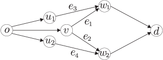
Figure 1: An SPE of $\Gamma$ may not induce an NE of $\Gamma^{n}$.

3 Existence of SPE

In this section, we establish the existence of an SPE for game $\Gamma=\Gamma(\bar{G})$ by using an algorithmic method. Given any feasible configuration $c_{r}$, our algorithm (Algorithm 1 below) computes a path profile, which is a special NE, of $\Gamma^{n}(c_{r})$. The special NEs computed for all configurations will assemble an SPE of $\Gamma$ in a way that for each configuration $c_{r}$ the path profile induced by $c_{r}$ and the SPE is exactly the NE computed for $\Gamma^{n}(c_{r})$.

The high-level idea behind our algorithm is a natural greedy best-response strategy: iteratively computing the unique best path based on all paths that have been obtained. Similar approaches with noticeable differences have been adopted to deal with various routing games, e.g., [15, 27, 32]. The special difficulties in our setting are imposed by subgames that start from any feasible configurations (which are essentially multi-origin problems) and priorities that are placed on edges rather than on players.

For any $S\subseteq\Delta(c_{r})$, we also use $\mbox{\boldmath$p$}=(P_{i})_{i\in S}$ with $P_{i}\in\mathcal{P}[o_{i}(c_{r}),d]$ to denote a partial path profile, corresponding to a (partial) routing. Given any vertex $v\in\bar{V}$, edge $uv\in\bar{E}$, and player $i\in S$,

• $t^{v}_{i}(\mbox{\boldmath$p$})$ (resp. $t^{uv}_{i}(\mbox{\boldmath$p$})$) denotes the time when $i$ reaches $v$ (resp. enters $uv$) under $p$;

• $t^{v}_{i}(\mbox{\boldmath$p$}):=\infty$ if $v\not\in P_{i}$, and $t^{uv}_{i}(\mbox{\boldmath$p$}):=\infty$ if $uv\notin P_{i}$.

If $S^{\prime}\subseteq S$, we often write $(P_{i})_{i\in S^{\prime}}$ as $\mbox{\boldmath$p$}_{S^{\prime}}$.

Given a feasible configuration $c_{r}$, our algorithm goes roughly as follows. Initially, let player subset $D$ of $\Delta(c_{r})$ and partial routing $\mbox{\boldmath$\pi$}_{D}$ of players in $D$ be empty. Then recursively, assuming players in $D$ go along their selected paths specified in $\mbox{\boldmath$\pi$}_{D}$, we enlarge $D$ with a new player $i\in\Delta(c_{r})\setminus D$ and an associated path $\Pi_{i}\in\mathcal{P}[o_{i}(c_{r}),d]$ in the following way. For each $j\in\Delta(c_{r})\setminus D$, define $\tau_{j}^{v}=\min\{t^{v}_{j}(\mbox{\boldmath$\pi$}_{D},R_{j})\,|\,R_{j}\in\mathcal{P}[o_{j}(c_{r}),d]\}$ as the “ideal latency” of player $j$ at vertex $v$ w.r.t. $\mbox{\boldmath$\pi$}_{D}$. Let $i\in\Delta(c_{r})\setminus D$ and $\Pi_{i}\in\mathcal{P}[o_{i}(c_{r}),d]$ be such that (i) $t^{d}_{i}(\mbox{\boldmath$\pi$}_{D},\Pi_{i})$ equals the smallest “ideal latency” at $d$ among all players in $\Delta(c_{r})\setminus D$, i.e., $t^{d}_{i}(\mbox{\boldmath$\pi$}_{D},\Pi_{i})=\min_{j\in\Delta(c_{r})\setminus D}\tau_{j}^{v}$, (ii) if there are more than one of such candidates $(i,\Pi_{i})$, then the choice of $(i,\Pi_{i})$ is made such that $\Pi_{i}$ has the highest priority w.r.t. $\prec_{d}$, (iii) if still more than one candidates satisfy (ii), in which case the paths involved must share the same ending edge and suppose $u$ is the tail vertex of this edge, then $t^{u}_{i}(\mbox{\boldmath$\pi$}_{D},\Pi_{i}[o_{i}(c_{r}),u])$ is the smallest. Repeat the above process until $o_{i}(c_{r})$ is reached, in which case all the remaining players must all queue at $e_{i}(c_{r})$ and $i$ is the head of this queue. The process is repeated while $D$ and $\mbox{\boldmath$\pi$}_{D}$ become larger and larger. A formal description of the process is presented in Algorithm 1.

Input: a feasible configuration $c_{r}$ at time $r$.

Output: the iterative dominating path profile (routing) $\mbox{\boldmath$\pi$}=(\Pi_{i})_{i\in\Delta(c_{r})}$ for $\Delta(c_{r})$ along with the corresponding player indices 1,2,….

• Initiate $D\leftarrow\emptyset$, $\mbox{\boldmath$\pi$}_{[0]}\leftarrow\emptyset$, $i\leftarrow 0$.

• $i\leftarrow i+1$ (NB: Start to search for a new dominator and his dominating path).

• For each player $j\in\Delta(c_{r})\setminus D$ and vertex $v\in\bar{G}$,

  • let $\tau_{j}^{v}=\min\{t^{v}_{j}(\mbox{\boldmath$\pi$}_{[i-1]},R_{j})\,|\,R_{j}\in\mathcal{P}[o_{j}(c_{r}),d]\}$ be the earliest time for $j$ to reach vertex $v$ from his current location in $c_{r}$, assuming that all other players in $\bar{G}$ are those in $D$ and they go along their paths specified in $\mbox{\boldmath$\pi$}_{[i-1]}$;

  • let $\mathcal{P}_{j}^{v}$ denote the set of all the corresponding $o_{j}(c_{r})$-$v$ paths for $j$ to reach $v$ at time $\tau_{i}^{v}$.

  • if there is no such path, then set $\tau_{j}^{v}\leftarrow\infty$ and $\mathcal{P}_{j}^{v}\leftarrow\emptyset$.

• $w\leftarrow d$, $D^{\prime}\leftarrow\Delta(c_{r})\setminus D$, $\Pi\leftarrow\emptyset$. (NB: Steps 3–10 are to help identify player $i$ and path $\Pi_{i}$ in Steps 11 and 12; $D^{\prime}$ holds the candidates for $i$; $\Pi$ is a subpath of $\Pi_{i}$ that will grow edge by edge starting from $d$.)

• While $\tau:=\min_{j\in D^{\prime}}\tau_{j}^{w}\geq r+1$ do

• $D^{\prime}\leftarrow\{j\in D^{\prime}\,|\,\tau_{j}^{w}=\tau\}$;

• let $uw$ be the edge of highest priority among all last edges of paths in $\cup_{j\in D^{\prime}}\mathcal{P}_{j}^{w}$;

• $\Pi\leftarrow\Pi\cup\{uw\}$;

• $w\leftarrow u$;

• End-While (NB: at the end of the while-loop all players in $D^{\prime}$ are queuing on the starting edge of $\Pi$ in configuration $c_{r}$)

• Let $i\in D^{\prime}$ be the player who stands first (among all players in $D^{\prime}$) in line on the starting edge of $\Pi$ in configuration $c_{r}$.

• Let $i$ select $\Pi_{i}\leftarrow\Pi$.

• $D\leftarrow D\cup\{i\}$, $\mbox{\boldmath$\pi$}_{[i]}\leftarrow(\mbox{\boldmath$\pi$}_{[i-1]},\Pi_{i})$. (NB: the algorithm outputs player $i$ and his path $\Pi_{i}$.)

• Go to Step 2.

ALGORITHM 1 (Iterative Dominating Path Profile)

It is worth noting that, for each $i\geq 1$, Algorithm 1 can identify player $i$ and path $\Pi_{i}$ in finite time via ignoring players and vertices that are sufficiently far from the origin $o$ in configuration $c_{r}$.

Suppose Algorithm 1 indexes the players of $\Delta(c_{r})$ as $1,2,\ldots$ with the associated path profile $\mbox{\boldmath$\pi$}=(\Pi_{1},\Pi_{2},\ldots)$. As can be seen from Lemma 1 below, each player $i\in\Delta(c_{r})$ is a dominator in $\Delta(c_{r})\setminus[i-1]$ and $\Pi_{i}$ is a dominating path w.r.t. $\mbox{\boldmath$\pi$}_{[i-1]}$ in the following sense: under the assumption that players in $[i-1]$ all follow $\mbox{\boldmath$\pi$}_{[i-1]}$, as long as $i$ takes $\Pi_{i}$, he will be among the first (within $\Delta(c_{r})\setminus[i-1]$) to reach the destination $d$ and no player in $\Delta(c_{r})\setminus[i]$ will be able to reach any of $\Pi_{i}$’s intermediary vertices earlier than $i$ does, regardless of the choices of players in $\Delta(c_{r})\setminus[i]$. We may also call the above $\mbox{\boldmath$\pi$}=(\Pi_{1},\Pi_{2},\ldots)$ an iterative dominating path profile.

Lemma 1.

Given any feasible configuration $c_{r}$ at time $r$, let players $1,2,\ldots$ of $\Delta(c_{r})$ be as indexed and path profile $\mbox{\boldmath$\pi$}=(\Pi_{i})_{i\in\Delta(c_{r})}$ be as computed in Algorithm 1. If players $i,j\in\Delta(c_{r})$ and player subset $S$ satisfy $j\in S\subseteq\Delta(c_{r})\setminus[i-1]$, then for any vertex $v\in\Pi_{i}$ and any path profile $p$ of $\Gamma^{n}(c_{r})$, it holds that

$$t_{i}^{v}(\mbox{\boldmath$\pi$}_{[i]},\mbox{\boldmath$p$}_{S\,\setminus\,\{i\}})=\min\{t_{i}^{v}(\mbox{\boldmath$\pi$}_{[i-1]},R_{i})\,|\,R_{i}\in\mathcal{P}[o_{i}(c_{r}),d]\}\leq t_{j}^{v}(\mbox{\boldmath$\pi$}_{[i-1]},\mbox{\boldmath$p$}_{S}).$$

The iterative dominance of $\pi$ particularly implies that given the selected paths in $\mbox{\boldmath$\pi$}_{[i-1]}$ of players in $[i-1]$, player $i$ has no incentive to deviate from $\Pi_{i}$ for each $i$, saying that $\pi$ is an NE of $\Gamma^{n}(c_{r})$. Furthermore, a special SPE of $\Gamma$ can be constructed, building on the iterative dominating path profiles for all feasible configurations.

Theorem 1.

Game $\Gamma$ admits an SPE.

Proof.

Given any history $h_{r}=(c_{0},\ldots,c_{r})\in\mathcal{H}_{r}$ for any time point $r\geq 0$, suppose the players in $\Delta(c_{r})$ are named as $1_{r},2_{r},\ldots$ such that player $i_{r}$ is the $i$th player added to $D$ in Step 13 of Algorithm 1 (with input $c_{r}$). For each player $i_{r}\in\Delta(c_{r})$, let $\Pi^{c_{r}}_{i_{r}}$ denote the path selected by $i_{r}$ in Algorithm 1; recall that under $c_{r}$ player $i$ queues at the first edge of $\Pi^{c_{r}}_{i_{r}}$. A configuration in $\mathcal{C}_{r+1}$ will result from $c_{r}$ according to action profile $\mbox{\boldmath$a$}^{c_{r}}$ defined as follows:

$$\text{The action of }i=\left\{\begin{array}[]{ll}\text{the first edge of }\Pi^{c_{r}}_{i_{r}},&\text{if $i$ queues after someone else;}\\ \emptyset,&\text{if $i$ queues first on the last edge of }\Pi^{c_{r}}_{i_{r}};\\ \text{the second edge of }\Pi^{c_{r}}_{i_{r}},&\text{otherwise}.\end{array}\right.$$

The set $\cup_{r\geq 0}\cup_{c_{r}\in\mathcal{C}_{r}}\mbox{\boldmath$a$}^{c_{r}}$ of action profiles defines a strategy profile $\sigma^{*}=(\sigma^{*}_{i})_{i\in\Delta}$ of $\Gamma$. We will prove that $\sigma^{*}$ is an SPE of $\Gamma$.

Let $(c_{r},c_{r+1},c_{r+2},\ldots)$ be the list of configurations and $(P^{*}_{i})_{i\in\Delta(c_{r})}$ be the path profile induced by $h_{r}$ and $\sigma^{*}$. It can be deduced from Lemma 1 and Algorithm 1 that

• For any $s\geq r+1$, player sequence $1_{s},2_{s},\ldots$ is a subsequence of $1_{s-1},2_{s-1},\ldots$ such that $\Delta(c_{s-1})\setminus\Delta(c_{s})$ consists of the first $|\Delta(c_{s-1})\setminus\Delta(c_{s})|$ players of $1_{s-1},2_{s-1},\ldots$

• For any $s\geq r+1$ and $i\in\Delta(c_{s})$, $\Pi^{c_{s}}_{i}\subseteq\Pi^{c_{s-1}}_{i}$.

Therefore, the path $P^{*}_{i}$ formed by the actions of each player $i\in\Delta(c_{r})$ is exactly $\Pi^{c_{r}}_{i}$. According to Lemma 1, we have, for any $i\geq 1$,

$\displaystyle t_{i_{r}}(\sigma^{*}|h_{r})=\min\{t^{d}_{i_{r}}(\Pi^{c_{r}}_{1_{r}},\ldots,\Pi^{c_{r}}_{(i-1)_{r}},P_{i_{r}})\,|\,P_{i_{r}}\in\mathcal{P}[o_{i_{r}}{(c_{r})},d]\}$ for each $i\geq 1$.

Moreover, for any $j\geq 1$ and any strategy profile $\sigma^{\prime}$ of $\Gamma$ with $\sigma^{\prime}_{i_{r}}=\sigma^{*}_{i_{r}}$ for all $i\in[j]$, the path profile $(P^{\prime}_{i})_{i\in\Delta(c_{r})}$ induced by $h_{r}$ and $\sigma^{\prime}$ satisfies $P^{\prime}_{i_{r}}=\Pi^{c_{r}}_{i_{r}}$ for all $i\in[j]$.

Now given any $k\geq 1$ and any $\sigma_{k_{r}}^{\prime}\in\Sigma_{k_{r}}$, we consider strategy profile $\sigma^{\prime}=(\sigma_{k_{r}}^{\prime},\sigma^{*}_{-k_{r}})$ and the path profile $\mbox{\boldmath$p$}^{\prime}=(P^{\prime}_{i})_{i\in\Delta(c_{r})}$ induced by $h_{r}$ and $\sigma^{\prime}$. We have $P^{\prime}_{i_{r}}=\Pi^{c_{r}}_{i_{r}}$ for all $i\in[k-1]$, and

$$t_{k_{r}}(\sigma^{\prime}_{k_{r}},\sigma^{*}_{-k_{r}}|h_{r})=t_{k_{r}}^{d}(\mbox{\boldmath$p$}^{\prime})=t_{k_{r}}^{d}(\Pi^{c_{r}}_{1_{r}},\ldots,\Pi^{c_{r}}_{(k-1)_{r}},\mbox{\boldmath$p$}^{\prime}_{\Delta(c_{r})\,\setminus\,\{1_{r},\ldots,(k-1)_{r}\}}).$$

It follows from Lemma 1 that

$t_{k_{r}}(\sigma^{\prime}_{k_{r}},\sigma^{*}_{-k_{r}}|h_{r})\geq\min\{t^{d}_{k_{r}}(\Pi_{1_{r}},\ldots,\Pi_{(k-1)_{r}},P_{k_{r}})\,|\,P_{k_{r}}\in\mathcal{P}[o_{k_{r}}(c_{r}),d]\}=t_{k_{r}}(\sigma^{*}|h_{r})$.

The arbitrary choices of $k$ and $\sigma^{\prime}_{k_{r}}$ imply that $\sigma^{*}$ is an SPE of $\Gamma$. ∎

We would like to remark that placing priorities on edges is crucial to the existence of an SPE. As the following example shows, the guarantee of SPE existence would be impossible if priorities were placed on players.

Example 2.

Consider a subgame starting with a configuration illustrated in Figure 2. There are 9 players in total represented by small rectangles on the edges, with players $i,j,k$ being our focus (the remaining 6 players do not need to make substantial decisions). The global priorities placed on the players are such that $i$ ranks higher than $j$ and $j$ higher than $k$. However, $k$ reaches $v_{1}$ (or $v_{2}$) one time unit earlier than $i$ (if they choose to pass the same vertex) and adds $1$ to the waiting time of $i$. Therefore, $i,j,k$ have a Rock-Paper-Scissors like relationship. It can be checked that this subgame does not have any NE. Since each of the three players $i,j,k$ only needs to make one decision, it follows that an SPE does not exist in this subgame.

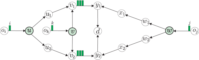
Figure 2: SPE might not exist if priorities were placed on players. In the subgame, player $i$ ranks higher than player $j$, and $j$ ranks higher than player $k$.

In contrast, the subgame in Figure 2 will have an NE if priorities are placed on edges as in our model. Suppose, e.g., $v_{1}y_{1}\prec_{y_{1}}x_{1}y_{1}$ and $x_{2}y_{2}\prec_{y_{2}}v_{2}y_{2}$, then it can be seen that the following implies an NE: $k$ chooses path $o_{k}vv_{1}y_{1}d$, $j$ chooses path $o_{j}ww_{2}x_{2}y_{2}d$, and $i$ makes an arbitrary choice. If in addition $y_{2}d\prec_{d}y_{1}d$, then

$$(v_{2}y_{2}d,v_{1}y_{1}d,v_{2}y_{2}d,v_{1}y_{1}d,v_{2}y_{2}d,v_{1}y_{1}d,o_{j}ww_{2}x_{2}y_{2}d,o_{k}vv_{1}y_{1}d,o_{i}uu_{2}v_{2}y_{2}d)$$

is the iteratively dominating path profile for the configuration.

4 Equilibria of interim games

Being natural and reasonable, models that are quite similar to $\Gamma^{n}$ have been the focus in the studies of dynamic traffic games [14, 27, 32]. While only special NEs were studied in the literature, we establish some general properties of all NEs of $\Gamma^{n}$. Using these properties, we prove that the NE outcomes of game $\Gamma^{n}$ form a proper subset of the SPE outcomes of game $\Gamma$. Therefore, $\Gamma^{n}$ can serve not only as an independent model but also as a technical approach that facilitates our analysis of the main game model $\Gamma$.

Given any configuration $c_{r}$ at time $r$, when studying some special SPE of game $\Gamma$ in Section 3, we obtain an iterative dominating path profile, which is a special NE of the interim game $\Gamma^{n}(c_{r})$, where players in $\Delta(c_{r})$ are completely ordered such that the ones with smaller indices have advantages over those with larger indices. For studying every NE of $\Gamma^{n}$, it turns out that batching players according to their arrival times at the destination $d$ is useful. For any NE $\pi$ of $\Gamma^{n}(c_{r})$, let $\tau(\mbox{\boldmath$\pi$},1)<\tau(\mbox{\boldmath$\pi$},2)<\tau(\mbox{\boldmath$\pi$},3)<\cdots$ be the arrival times of all players in $\Delta(c_{r})$ at $d$ under $\pi$. For each integer $k\geq 1$, let

$$\Delta(\mbox{\boldmath$\pi$},k):=\{i\in{\Delta(c_{r})}\,|\,t^{d}_{i}(\mbox{\boldmath$\pi$})=\tau(\mbox{\boldmath$\pi$},k)\}$$

be the set of players in $\Gamma^{n}(c_{r})$ who reach $d$ at the $k$th earliest time, i.e., $\tau(\mbox{\boldmath$\pi$},k)$ under $\pi$; we often refer to $\Delta(\mbox{\boldmath$\pi$},k)$ as the $k$th batch. We use

$$\Delta(\mbox{\boldmath$\pi$},{[k]}):=\cup_{j\in[k]}\Delta(\mbox{\boldmath$\pi$},j)$$

to denote the set of players reaching $d$ no later than $\tau(\mbox{\boldmath$\pi$},k)$, i.e., those in the first $k$ batches. For notational convenience, we set $\Delta(\mbox{\boldmath$\pi$},[0]):=\emptyset$ to be the $0$th batch, and let $\Delta(\mbox{\boldmath$\pi$},[\infty]):=\Delta(c_{r})$ denote the disjoint union of all batches.

4.1 A motivating example

In studying NE of $\Gamma^{n}$, we need to frequently analyze what happens if one player unilaterally deviates by choosing a different path. This is a quite tricky issue in general. Players may affect one another in quite unexpected ways. As the following extreme example shows, adding a player to the system may weakly improve the performances of other players (nobody is worse off and at least one is better off), or equivalently, removing a player may weakly harm the performances of other players.

Example 3.

The configuration $c_{r}$ at time $r$ is as depicted in Figure 3. There are 10 players (shown as small rectangles on edges) in total, with $i,j,k$ being our focus (note that Figure 3 shows only a part of the whole network). Edge $e_{1}$ has a higher priority than $e_{2}$. Let player $k$ choose the top path $u_{1}u_{2}u_{3}u_{4}u_{5}d$, player $i$ choose the middle path $u_{1}u_{2}v_{3}v_{4}d$, and player $j$ follow the bottom path $v_{1}v_{2}v_{3}v_{4}v_{5}d$. It can be checked that all the three players reach $d$ at time $r+5$ (and the three chosen paths along with the trivial paths of the other 7 players constitute an NE for $\Gamma^{n}(c_{r})$). Suppose now player $k$ is removed from the system, and $i$ and $j$ keep their chosen paths. This removing makes $i$ arrive at vertices $u_{2}$, $v_{3}$ and $v_{4}$ one unit of time earlier. Since $i$ has to pay one extra unit of waiting cost on edge $v_{4}d$, he reaches $d$ still at time $r+5$. However, the earlier arrival of $i$ at $v_{3}$ delays $j$, making him reach $d$ at time $r+6$. Note that both path profiles are NEs.

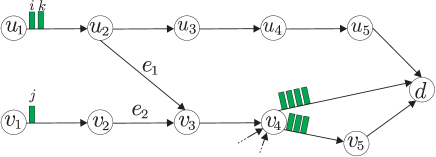
Figure 3: Removing a player (weakly) harms the performances of other players.

4.2 A critical lemma

Throughout this subsection, we fix a strategy profile $\mbox{\boldmath$\alpha$}=(A_{i})_{i\in\Delta(c_{r})}$ of $\Gamma^{n}(c_{r})$ and consider a fixed player $\zeta\in\Delta(c_{r})$ and the scenario where only player $\zeta$ changes his strategy. Let $\mbox{\boldmath$\alpha$}_{-\zeta}=(A_{i})_{i\in\Delta(c_{r})\setminus\{\zeta\}}$ denote the partial strategy profile of players in $\Delta(c_{r})$ other than $\zeta$. For each vertex $v$, define

$$\tau^{v}:=\min_{A^{\prime}_{\zeta}\in\mathcal{P}[o_{\zeta}(c_{r}),d]}\{t_{\zeta}^{v}(A^{\prime}_{\zeta},\mbox{\boldmath$\alpha$}_{-\zeta})\}$$

as the earliest time at which player $\zeta$ can reach vertex $v$ by unilaterally changing his path (if there is no path from $o_{\zeta}(c_{r})$ to $v$, then set $\tau^{v}:=+\infty$). Analogously, for each player $j\in\Delta(c_{r})\setminus\{\zeta\}$ and vertex $v\in A_{j}$, define

$$\tau_{j}^{v}:=\min_{A^{\prime}_{\zeta}\in\mathcal{P}[o_{\zeta}(c_{r}),d]}\{t_{j}^{v}(A^{\prime}_{\zeta},\mbox{\boldmath$\alpha$}_{-\zeta})\}$$

as the earliest time at which player $j$ can reach vertex $v$ when player $\zeta$ unilaterally changes his path. We emphasize that $j$ keeps his path at $A_{j}$ in the definition of $\tau_{j}^{v}$.

In the following, for any non-degenerated path $P$ in $\bar{G}$ and vertex $v\in P$, we use $e_{v}(P)$ to denote the edge with head $v$ in $P$.

Definition 3.

For every player $j\in\Delta(c_{r})\setminus\{\zeta\}$ and vertex $v\in A_{j}$, we say player $\zeta$ dominates player $j$ at vertex $v$ under $\alpha$ if

• $\tau^{v}<\tau_{j}^{v}$; or

• $\tau^{v}=\tau_{j}^{v}$, and there exists an $o_{\zeta}(c_{r})$-$v$-$d$ path $A^{*}_{\zeta}$ such that $t_{\zeta}^{v}(A^{*}_{\zeta},\mbox{\boldmath$\alpha$}_{-\zeta})=\tau^{v}$ and $e_{v}(A^{*}_{\zeta})\preceq_{v}e_{v}(A_{j})$.

In words, player $\zeta$ dominates $j$ at $v$ if and only if either the earliest possible time that $\zeta$ reaches $v$ is earlier than the earliest possible time that $j$ reaches $v$, or the two earliest arrival times are equal and $\zeta$ has a corresponding path that allows him to enter $v$ from an edge with a higher or equal priority over the edge taken by $j$, assuming that only $\zeta$ is allowed to deviate his path from the given path profile $\alpha$.

Lemma 2.

For any player $j\in\Delta(c_{r})\setminus\{\zeta\}$ and vertex $v\in A_{j}$, if there exists a path $A^{\prime}_{\zeta}\in\mathcal{P}[o_{\zeta}(c_{r}),d]$ such that $t_{j}^{v}(A^{\prime}_{\zeta},\mbox{\boldmath$\alpha$}_{-\zeta})\neq t_{j}^{v}(\mbox{\boldmath$\alpha$})$, i.e., player $\zeta$ can influence player $j$’s arrival time at $v$ by unilaterally changing his path, then $\zeta$ dominates $j$ at $v$.

The above lemma implies in particular that if player $\zeta$ can influence the arrival time of player $j$ at vertex $v$, then $\zeta$ is able to reach $v$ earlier than $j$ does. Note that this result would be impossible if priorities were placed on players, which can be seen from Figure 2. We focus on player $k$ and suppose the path profile $\alpha$ is such that $i$ and $j$ both choose their upper paths and $k$ chooses his lower path. Then $k$ is able to influence player $j$’s arrival time at node $y_{1}$ by deviating to the upper path. However, $k$ is unable to reach $y_{1}$ earlier than $j$ does.

From the proof of Lemma 2, we also have the following stronger result.

Corollary 1.

If player $\zeta$ dominates some player $j\in\Delta(c_{r})\setminus\{\zeta\}$ at vertex $v\in A_{j}$, then $\zeta$ dominates $j$ at all the other vertices on the subpath $A_{j}[v,d]$.

As an immediate result of Corollary 1, we have the following lemma.

Lemma 3.

Let $\mbox{\boldmath$\pi$}=(\Pi_{i})_{i\in{\Delta(c_{r})}}$ be an NE of $\Gamma^{n}(c_{r})$. For every $k\geq 1$ and every player $j\in\Delta(c_{r})\setminus\Delta(\mbox{\boldmath$\pi$},[k])$, $j$ cannot dominate any player $i\in\Delta(\mbox{\boldmath$\pi$},[k])$ at any vertex of path $\Pi_{i}$.

Proof.

Suppose on the contrary that there does exist a player $j\in\Delta(c_{r})\setminus\Delta(\mbox{\boldmath$\pi$},[k])$ and player $i\in\Delta(\mbox{\boldmath$\pi$},[k])$ such that $j$ dominates $i$ at some vertex $v\in\Pi_{i}$. Then by Corollary 1, $j$ also dominates $i$ at vertex $d$. This means that there exists a path $\Pi_{j}^{*}$ such that

$$t_{j}^{d}(\Pi_{j}^{*},\mbox{\boldmath$\pi$}_{-j})\leq\min_{\Pi_{j}^{\prime}\in\mathcal{P}[o_{j}(c_{r}),d]}\{t_{i}^{d}(\Pi_{j}^{\prime},\mbox{\boldmath$\pi$}_{-j})\}\leq t_{i}^{d}(\mbox{\boldmath$\pi$})=\tau(\pi,k).$$

However, $t^{d}_{j}(\mbox{\boldmath$\pi$})>\tau(\mbox{\boldmath$\pi$},k)$ due to $j\in\Delta(c_{r})\setminus\Delta(\mbox{\boldmath$\pi$},[k])$, indicating that $j$ has an incentive to deviate to $\Pi_{j}^{*}$ and hence violating the fact that $\pi$ is an NE. ∎

4.3 Computing the earliest-arrival best response

For any configuration $c_{r}$ and the corresponding normal-form game $\Gamma^{n}(c_{r})$, suppose now we are given a path profile $\alpha$. We show in this subsection how to compute a special best-response defined below.

Definition 4.

Given a partial path profile $\mbox{\boldmath$\alpha$}_{-\zeta}$, an $o_{\zeta}(c_{r})$-$d$ path $P^{*}$ of player $\zeta\in\Delta(c_{r})$ is called the earliest-arrival best response if (i) $\zeta$ arrives at each node of $P^{*}$ the earliest among all $o_{\zeta}(c_{r})$-$d$ paths, and (ii) when there are more than one earliest ways to arrive at a node of $P^{*}$, $P^{*}$ always selects an entering edge with the highest priority.

We shall see that the earliest-arrival best response exists and is unique. Observe that each dominating path computed in Algorithm 1 is an earliest-arrival best response. It can also be seen that, when all players take the earliest-arrival best response to each other in $\alpha$, then $\alpha$ is exactly the NE computed in Algorithm 1.

We find that the earliest-arrival best responses can be computed via a dynamic programming that resembles the classical Dijkstra’s algorithm for the shortest-path problem. This algorithm is polynomial when $\Delta(c_{r})$ is finite. Note that there may well be best-responses that are not earliest-arrival. However, the earliest-arrival best response possesses several nice properties that are not owned by general best responses.

Under the path profile $\alpha$, for any edge $e=uv$, recall that $Q_{e}^{t}$ is the set of players queuing on edge $e$ at time $t\geq r$. For an edge $e^{\prime}=wu$ whose ending vertex $u$ is the starting one of $e$, we use

$$Q_{e}^{t}(t,e^{\prime})\subseteq Q_{e}^{t}$$

to denote the subset of players in $Q_{e}^{t}$ who entered $e=uv$ at time $t$ and from edges with priorities no higher than $e^{\prime}=wu$. For any vertex $v\in\bar{V}$ with $\tau^{v}\neq 0$, denote $e^{*}(v)$ as the edge with the highest priority w.r.t vertex $v$ that $\zeta$ can use to reach $v$ at time $\tau^{v}$. Initially, we set $Q_{e}^{r}(r,e^{*}(o_{\zeta}(c_{r})))$ as the set of players in $Q_{e}^{r}$ that queue after $\zeta$ when $e=e_{\zeta}(c_{r})$, where $e_{\zeta}(c_{r})$ is the initial edge that $\zeta$ rests on in $c_{r}$.

Lemma 4.

For any vertex $v\in\bar{V}$, if $\tau^{v}\neq\infty$, then

$$\tau^{v}=\min_{uv\in\bar{E}^{-}(v)}\Big{\{}\tau^{u}+1+|Q_{uv}^{\tau^{u}}|-|Q_{uv}^{\tau^{u}}(\tau^{u},e^{*}(u))|\Big{\}}$$

and

$$e^{*}(v)=\arg\min_{uv\in\bar{E}^{-}(v)}\!\!\!{}^{*}\Big{\{}\tau^{u}+1+|Q_{uv}^{\tau^{u}}|-|Q_{uv}^{\tau^{u}}(\tau^{u},e^{*}(u))|\Big{\}},$$

where $\arg\min^{*}$ selects the edge with the highest priority among all those achieving the minimum.

Suppose now $\Delta(c_{r})$ is finite. Then, the values of $Q_{e}^{t}$ and $Q_{e}^{t}(t,e^{\prime})$ are polynomially computable through simulating the traffic process. Therefore, the earliest-arrival best response of each player is polynomially computable in this case.

4.4 NE properties

The following lemma is very powerful. It helps us to show that the interactions between players of different batches at an NE are relatively clear and hierarchal, bearing many similarities to those in the special SPE studied in Section 3 and Appendix A.3.

Lemma 5.

Let $\pi$ be an NE of $\Gamma^{n}(c_{r})$. For any batch index $k\geq 1$, player $i\in B:=\Delta(\mbox{\boldmath$\pi$},[k])$, vertex $v\in\Pi_{i}$, player $j\in\Delta(c_{r})\setminus B$, and partial path profile $r$ for players in $\Delta(c_{r})\setminus B$, it holds that

$$t^{v}_{i}(\mbox{\boldmath$\pi$})=t^{v}_{i}(\mbox{\boldmath$\pi$}_{B},\mbox{\boldmath$r$})\leq t^{v}_{j}(\mbox{\boldmath$\pi$}_{B},\mbox{\boldmath$r$})\mbox{ and }t_{j}^{d}(\mbox{\boldmath$\pi$}_{B},\mbox{\boldmath$r$})\geq\tau(\mbox{\boldmath$\pi$},k+1)>t_{i}^{d}(\mbox{\boldmath$\pi$}_{B},\mbox{\boldmath$r$}).$$ (4.1)

One of our main results in this section is the following theorem. Recall that a strong NE is an NE such that no subset of players are able to strictly better off via group deviation.

Theorem 2.

Let $\pi$ be an NE of $\Gamma^{n}(c_{r})$. The following properties are satisfied.

• Hierarchal Independence. If players in a batch and those in earlier batches all follow their equilibrium strategies as in $\pi$, then their arrival times at any vertex are independent of other players’ strategies.

• Hierarchal Optimality. The latency of each player in the first batch $\Delta(\mbox{\boldmath$\pi$},1)$ is the smallest among the latencies of all players under any routing of $\Gamma^{n}(c_{r})$. In general, for all $k\geq 2$, the latency of each player in the $k$th batch $\Delta(\mbox{\boldmath$\pi$},k)$ is the smallest among the latencies of all players in $\Delta(c_{r})\setminus\Delta(\mbox{\boldmath$\pi$},[k-1])$ under any routing of $\Gamma^{n}(c_{r})$ in which players in the first $k-1$ batches $\Delta(\mbox{\boldmath$\pi$},[k-1])$ follow their routes specified by $\pi$.

• Global FIFO. Under $\pi$, if there exists a vertex $v\in\bar{V}$ (particularly the origin $o$) such that player $i$ reaches $v$ earlier than $j$ does or they reach $v$ at the same time but $i$ comes from an edge with a higher priority than $j$ does, then $i$ reaches the destination $d$ no later than $j$ does.

• Strong NE. In $\Gamma^{n}(c_{r})$, every NE is also a strong NE. That is, in any NE of $\Gamma^{n}(c_{r})$, no set of players can be strictly better off by deviating together to other paths. In particular, this means that each NE of $\Gamma^{n}(c_{r})$ is weakly Pareto Optimal.

4.5 Equilibrium relationship between $\Gamma$ and $\Gamma^{n}$

In this subsection, we establish in a constructive way that each NE outcome of $\Gamma^{n}$ is an SPE outcome of $\Gamma$. Given any NE $\pi$ of $\Gamma^{n}$, we construct for every history $h_{r}=(c_{0},\ldots,c_{r})$, $r\geq 0$, an NE $\mbox{\boldmath$\pi$}(h_{r})$ of interim game $\Gamma^{n}(c_{r})$ with the particular setting $\mbox{\boldmath$\pi$}(h_{0}):=\mbox{\boldmath$\pi$}$. Then, we construct an SPE of $\Gamma$ by assembling these NEs such that starting from any history $h_{r}$ ($r\geq 0)$ the outcome of the SPE is exactly the NE $\mbox{\boldmath$\pi$}(h_{r})$. (Note that the reference of each NE constructed is a history rather than a configuration. Since different histories may have the same ending configuration, we may construct multiple NEs for the same interim game.)

Such an NE-based assembling is more difficult than the one in Section 3, which constructs a special SPE restricted to nothing. What is more complicated here is that we are unable to design a Markovian SPE (cf. Appendix A.3). In particular, the natural idea of constructing the NEs $\mbox{\boldmath$\pi$}(h_{r})$, $r\geq 1$ rather than $\mbox{\boldmath$\pi$}(h_{0})=\mbox{\boldmath$\pi$}$ directly using Algorithm 1 does not work, because, e.g., players not in the first batch under $\pi$ may have incentives to deviate at the game tree root.

Our construction of the NEs is done iteratively on the game tree of $\Gamma$ from the root $h_{0}=(c_{0})$. Initially, the constructed NE $\mbox{\boldmath$\pi$}(h_{0})$ for $h_{0}$ is simply $\pi$. For each $r\geq 1$, suppose inductively that for a history $h_{r-1}=(c_{0},\ldots,c_{r-1})\in\mathcal{H}_{r-1}$, the NE $\mbox{\boldmath$\pi$}(h_{r-1})$ of game $\Gamma^{n}(c_{r-1})$, written for convenience as $\mbox{\boldmath$\rho$}=(P_{i})_{i\in\Delta(c_{r-1})}$, has been constructed. We construct below the NE $\mbox{\boldmath$\pi$}(h_{r})$, denoted $\mbox{\boldmath$\rho$}^{\prime}=(P^{\prime}_{i})_{i\in\Delta(c_{r})}$, for each child history $h_{r}=(c_{0},\ldots,c_{r-1},c_{r})$ of $h_{r-1}$. Suppose that

• $(e_{i})_{i\in\Delta(c_{r-1})}$ is the action profile at game tree node $h_{r-1}$ determined by $\rho$, i.e, no action in the profile deviates from $\rho$, and

• $(e^{\prime}_{i})_{i\in\Delta(c_{r-1})}$ is the action profile that leads history $h_{r-1}$ to its child history $h_{r}$ (or equivalently leads $c_{r-1}$ to $c_{r}$).

We construct $\mbox{\boldmath$\rho$}^{\prime}$ in two steps as follows.

CONSTRUCTION I: Let $\Bbbk\geq 0$ be the maximum nonnegative integer such that the action of each player of $\Delta(\mbox{\boldmath$\rho$},[\Bbbk])$ under $(e^{\prime}_{i})_{i\in\Delta(c_{r-1})}$ is the same as under $(e_{i})_{i\in\Delta(c_{r-1})}$, i.e.,

$$\Bbbk:=\sup\{k\,|\,e_{i}=e_{i}^{\prime}\text{ for all }i\in\Delta(\mbox{\boldmath$\rho$},[k])\}.$$ (4.2)

(Note that it is possible $\Bbbk=0$ with $\Delta(\mbox{\boldmath$\rho$},[0])=\emptyset$ or $\Bbbk=\infty$ with $\Delta(\mbox{\boldmath$\rho$},[\infty])=\Delta(c_{r-1})$.) We let players in the first $\Bbbk$ batches who are still in the system at time $r$ under $\rho$ keep their paths under $\mbox{\boldmath$\rho$}^{\prime}$. To be more specific, we set

$$P_{i}^{\prime}:=P_{i}[o_{i}(c_{r}),d]\text{ for all }i\in\Delta(\mbox{\boldmath$\rho$},[\Bbbk])\cap\Delta(c_{r}).$$ (4.3)

CONSTRUCTION II: Based on the equilibrium strategies kept for players in $\Delta(\mbox{\boldmath$\rho$},[\Bbbk])\cap\Delta(c_{r})$ as specified in (4.3), which particularly guarantees invariant arrival times at any vertex for these players regardless of other players’ choices (see the hierarchal independence in Theorem 2(i)), we find an iterative dominating path profile $(P^{\prime}_{i})_{i\in\Delta(c_{r})\setminus\Delta(\mbox{\boldmath$\rho$},[\Bbbk])}$ for the remaining players, using a process that is more general than Algorithm 1 (see Appendices A.2 and B.4 for more details).

Intuitively, $\mbox{\boldmath$\rho$}^{\prime}$ is a combination of a part of $\rho$ and an iterative dominating partial path profile. It can be shown that the constructed $\mbox{\boldmath$\rho$}^{\prime}$ is indeed an NE of $\Gamma^{n}(c_{r})$ (see Lemma 13 in the Appendix), which completes our inductive construction. Furthermore, the partial hierarchal independence and iterative domination guaranteed by Constructions I and II enable us to accomplish our task of assembling all the NEs constructed into an SPE of $\Gamma$.

Theorem 3.

If $\pi$ is an NE of game $\Gamma^{n}$, then there exists an SPE $\sigma$ of game $\Gamma$, such that the path profile induced by the initial history $h_{0}$ and $\sigma$ is exactly $\pi$.

Combining with Example 1, the above theorem shows that the NE outcome set of $\Gamma^{n}$ is typically a proper subset of the SPE outcome set of $\Gamma$, reaffirming an intuition that model $\Gamma$ is more flexible than $\Gamma^{n}$. Since model $\Gamma^{n}$ is relatively easier to study, also natural and more frequently analyzed in the literature, Theorem 3 can serve as a useful bridge between $\Gamma$ and $\Gamma^{n}$.

5 Bounding equilibrium queue lengths

In this section, we consider two classes of networks, and prove that the queue lengths at any NE of the game $\Gamma^{n}(G)$ are bounded above by a finite number that only depends on the number $m=|E|$ of edges in $G$, provided that the inflow size never exceeds the network capacity.

Definition 5.

A network $G$ with origin $o$ and destination $d$ is $o$-$d$ series-parallel or simply series-parallel if

• $G$ consists of a single edge $od$; or

• $G$ is obtained by connecting two smaller $o_{i}$-$d_{i}$ series-parallel networks $G_{i}$, $i=1,2$, in series — identifying $d_{1}$ and $o_{2}$, and naming $o_{1}$ as $o$, and $d_{2}$ as $d$; or

• $G$ is obtained by connecting two smaller $o_{i}$-$d_{i}$ series-parallel networks $G_{i}$, $i=1,2$, in parallel — identifying $o_{1}$ and $o_{2}$ to form $o$ and identifying $d_{1}$ and $d_{2}$ to form $d$.

We reserve $L$ for the length of a longest $o$-$d$ path in $G$, and $\Lambda$ for the maximum in-degree of vertices in $G$. Then clearly, $\max\{L,\Lambda\}\leq m$. The following observation is trivial but important.

Observation 1.

Under any routing, at most $\Lambda$ players can reach the same vertex (in particular, the destination $d$) at the same time.

In view of Definition 5, the series-parallel network $G$ is obtained from $m$ edges by performing a sequence of $m-1$ series or parallel connection operations. Each of these operations connects two series-parallel subnetworks $G_{1}$ and $G_{2}$ of $G$ into a bigger series-parallel subnetwork $G_{3}$ of $G$. Fix any such sequence of $m-1$ connection operations that leads to $G$ and let $\mathfrak{S}$ be the set of all the subnetworks $G_{1}$, $G_{2}$ and $G_{3}$ that appear during the whole process of the sequence of $m-1$ connection operations. Then clearly,

$G\in\mathfrak{S}$ and $|\mathfrak{S}|=2m-1$.

Henceforth, we study an arbitrary NE, denoted as $\mbox{\boldmath$\pi$}=(\Pi_{i})_{i\in\Delta}$, of game $\Gamma^{n}$. For each player $i\in\Delta$ and each vertex $v\in\Pi_{i}$, we use $\Delta^{v}_{i}:=\{j\in\Delta\,|\,t^{v}_{j}(\mbox{\boldmath$\pi$})=t^{v}_{i}(\mbox{\boldmath$\pi$})\}$ to denote the set of players in $\Delta$ who reach $v$ under $\pi$ at the same time as $i$ does. Note from Observation 1 that

$$|\Delta^{v}_{i}|\leq\Lambda\text{ for every }i\in\Delta\text{ and each vertex }v\in\Pi_{i}.$$

Using the observation and global FIFO property in Theorem 2(iii), we can upper bound the ratio between the population sizes in any pair of subnetworks connecting in parallel, as the following lemma states.

Lemma 6.

Suppose that $G_{1},G_{2}\in\mathfrak{S}$ are connected in parallel to form a series-parallel network in $\mathfrak{S}$. Under $\pi$ and at any time point $t$, if $G_{1}$ and $G_{2}$ accommodate $n_{1}$ and $n_{2}$ players respectively, then $n_{i}\leq 2\Lambda L(2\Lambda+n_{j})\leq 2m^{2}(2m+n_{j})$ for $\{i,j\}=\{1,2\}$.

By an $o$-$d$ cut or simply a cut of $G$ we mean a set of edges whose removal from $G$ leaves the graph unconnected from $o$ to $d$. We say that a minimal cut of $G$ is full at time $t$ if each edge of the cut has some player on it at time $t$ (i.e., there is a nonempty queue at each edge). Let $C=\{e_{1},\ldots,e_{k}\}$ and $C^{\prime}=\{e^{\prime}_{1},\ldots,e^{\prime}_{k}\}$ be two minimum cuts of $G$. We say that $C$ is on the left of $C^{\prime}$ if for each $i\in[k]$ there exists an $o$-$d$ path in $G$ which contains $e_{i},e^{\prime}_{i}$ and visits $e_{i}$ before $e^{\prime}_{i}$.

For any $o^{\prime}$-$d^{\prime}$ series-parallel network $G^{\prime}$, let $\Xi(G^{\prime})$ denote the leftmost minimum $o^{\prime}$-$d^{\prime}$ cut of $G^{\prime}$. In particular, $|\Xi(G^{\prime})|$ is the minimum cut size of $G^{\prime}$. The cut $\Xi(G^{\prime})$ partitions $G^{\prime}$ into two parts: the left part $G^{\prime l}$ that contains $o^{\prime}$, and the right $G^{\prime r}$ that contains $d^{\prime}$.

Definition 6.

Let $\mathfrak{F}$ denote the set of series-parallel subnetworks $G_{i}\in\mathfrak{S}$ such that there exist finite integers $F^{l}_{i}$ and $F^{r}_{i}$ satisfying the following two conditions (for any inflow):

• $\Xi(G_{i})$ is full as long as $G_{i}^{l}$ accommodates more than $F^{l}_{i}$ players, and

• $G_{i}^{r}$ can accommodate at most $F^{r}_{i}$ players at any time.

First, we can see the set $\mathfrak{F}$ is nonempty because every single edge apparently belongs to $\mathfrak{F}$. In the two lemmas below, we are given $G_{1},G_{2}\in\mathfrak{F}$, such that $G_{i}$ is an $o_{i}$-$d_{i}$ series-parallel network for $i=1,2$.

Lemma 7.

If $G_{s}\in\mathfrak{S}$ is the combination of $G_{1}$ and $G_{2}$ in series, then $G_{s}\in\mathfrak{F}$.

Lemma 8.

If $G_{p}\in\mathfrak{S}$ is the combination of $G_{1}$ and $G_{2}$ in parallel, then $G_{p}\in\mathfrak{F}$.

Proof.

It is clear that $\Xi(G_{p})=\Xi(G_{1})\cup\Xi(G_{2})$, $G^{l}_{p}=G^{l}_{1}\cup G_{2}^{l}$, and $G^{r}_{p}=G^{r}_{1}\cup G_{2}^{r}$. Therefore, $G^{r}_{p}$ accommodates at most $F_{p}^{r}\equiv F^{r}_{1}+F^{r}_{2}$ players at any time. To prove $G_{p}\in\mathfrak{F}$, we only need to show that $\Xi(G_{1})\cup\Xi(G_{2})$ is full as long as $G^{l}_{1}\cup G_{2}^{l}$ accommodates more than a certain finite number of players. As $G_{1},G_{2}\in\mathfrak{F}$, it suffices to consider the time $t$ when one of $G^{l}_{1}$ and $G_{2}^{l}$, say $G^{l}_{1}$, accommodates at most $F^{l}_{1}$ players. Suppose that $G_{2}^{l}$ accommodates $F$ players at time $t$. It follows from Lemma 6 that $G_{1}$ accommodates at least $F/(2m^{2})-2m$ players at time $t$. As $G_{1}\in\mathfrak{F}$, there are at least $F/(2m^{2})-2m-F^{r}_{1}$ players inside $G_{1}^{l}$ at time $t$. It follows from $F/(2m^{2})-2m-F^{r}_{1}\leq F^{l}_{1}$ that $F\leq 2m^{2}(2m+F^{l}_{1}+F^{r}_{1})$. ∎

Theorem 4.

Let $G$ be a series-parallel network. If $|\Delta_{t}|\leq|\Xi(G)|$ for all $t\geq 1$, then there exists a finite number such that, for any NE of $\Gamma^{n}(G)$, the number of players in $G$ is upper bounded by this number, implying that the latency of any player at any NE is upper bounded.

Proof.

Since $|\mathfrak{S}|=2m-1$, combining Lemmas 7 and 8, an inductive argument shows that $\mathfrak{S}=\mathfrak{F}$. In particular, $G\in\mathfrak{F}$ says that $\Xi(G)$ is full as long as $G^{l}$ accommodates more than $F^{l}$ players, and $G^{r}$ can accommodate at most $F^{r}$ players at any time, where $F^{l}$ and $F^{r}$ are finite numbers. Similar to the argument used in the proof of Lemma 7, we consider any time point $t$ such that $G^{l}$ accommodates at most $F^{l}$ players at time $t$, and more than $F^{l}$ players at time $t+1$. Then $G^{l}$ accommodates at most $F^{l}+|\Delta_{t+1}|\leq F^{l}+|\Xi(G)|$ players and $\Xi(G)$ is full at time $t+1$. Thus $|\Xi(G)|$ players leave $G^{l}$ at time $t+2$ while $|\Delta_{t+2}|$ ($\leq|\Xi(G)|$) players enter $G^{l}$. It follows that the number of players inside $G^{l}$ is nonincreasing unless the number decreases below $F^{l}+1$. Therefore, at any time $G^{l}$ can accommodate at most $F^{l}+|\Xi(G)|$ players, and $G$ can accommodate at most $F^{l}+|\Xi(G)|+F^{r}$ players. This also means the total latency for any player travelling from $o$ to $d$ under any NE is bounded by a finite number since any queue length is upper bounded by the finite number $F^{l}+m+F^{r}$. ∎

If we take the average traveling time from $o$ to $d$ for all players as a measure of the social welfare as in [27], then the boundedness of the queues implies the PoA of game $\Gamma^{n}(G)$ is also bounded. By Theorem 3, this means that the PoS of game $\Gamma(G)$ is also bounded.

In closing this section, we establish boundedness of any SPE queue lengths for another type of networks.

Theorem 5.

Given a dynamic routing game $\Gamma$ on an acyclic network $G=(V,E)$ with origin $o$ and destination $d$, suppose $|E^{+}(v)|\geq|E^{-}(v)|$ for any vertex $v\in V\setminus\{o,d\}$. Let $\sigma$ be any SPE of game $\Gamma(G)$. If the inflow size $|\Delta_{r}|$ never exceeds the size of a minimum $o$-$d$ cut of $G$, then there exists a finite number $U$ depending only on $|E|$ such that $t_{i}(\sigma)\leq U$ all $i\in\Delta$.

6 Concluding remarks

In this paper, we have studied an atomic network congestion game of discrete-time dynamic traffic. This is a relatively unexplored area in the study of congestion games. The most prominent feature of our model is the great flexibility agents enjoy so as to make online decisions at all intermediary vertices and, accordingly, SPE serves as the default solution concept. We have shown that this more flexible model has close connections with the corresponding game of normal form, which is more often studied in the literature. We have identified many surprisingly nice properties of the NE flows of the latter model, the equivalence between NEs and strong NEs and a global FIFO, to name a few.

This paper is our first attempt in understanding the consequences of the introduction of agents’ flexibility of online decision making in dynamic traffic games. Many interesting problems are widely open. For example, is there an upper bound on the SPE (or NE) queue lengths for general networks? What are more accurate bounds on PoA and PoS w.r.t. either NEs or SPEs? Does a long-run steady state exist when the inflow is constant or seasonal? How efficient is this steady state if it does exist? What if agents have multi-origins and multi-destinations? What if agents are allowed to choose their departure times? Exploring these problems will undoubtedly help us better understand atomic games of dynamic traffic.

Appendix

Appendix A Details in Section 3

A.1 Iterative dominations

To facilitate our discussions, the proof of Lemma 1 in particular, we introduce several notations. Given any (directed) path $P$ in $\bar{G}$, and vertices $a,b$ in $P$ such that $a$ is passed no later than $b$ by path $P$, we use $P[a,b]$ to denote the sub-path of $P$ from $a$ to $b$. We write $P(a,b]=P[a,b]\setminus\{a\}$, $P[a,b)=P[a,b]\setminus\{b\}$ and $P(a,b)=P[a,b]\setminus\{a,b\}$.

Given any feasible configuration $c_{r}$ at time $r$, let players $1,2,\ldots$ of $\Delta(c_{r})$ be as indexed and path profile $\mbox{\boldmath$\pi$}=(\Pi_{i})_{i\in\Delta(c_{r})}$ be as computed in Algorithm 1. For any player indices $i,j$ with $i<j$ and any vertex $v\in\bar{G}$, let

$$\tau_{j}^{v}\llbracket i\rrbracket:=\min\{t_{j}^{v}(\mbox{\boldmath$\pi$}_{[i]},R_{j})\,|\,R_{j}\in\mathcal{P}[o_{j}(c_{r}),d]\}$$ (A.1)

denote the value $\tau^{v}_{j}$ computed for player $j$ in Step 3 at the $(i+1)$th iteration of Algorithm 1, i.e., the earliest time for player $j$ to reach vertex $v$ starting from edge $e_{j}(c_{r})$, based only on the partial routing $\mbox{\boldmath$\pi$}_{[i]}$ of players in $[i]$.

Lemma 9 (Restatement of Lemma 1).

Let player indices $i,j$ and player subset $S$ satisfy $j\in S\subseteq\Delta(c_{r})\setminus[i-1]$. Then

$$t_{i}^{v}(\mbox{\boldmath$\pi$}_{[i]},\mbox{\boldmath$p$}_{S\,\setminus\,\{i\}})=\tau_{i}^{v}\llbracket i-1\rrbracket\leq t_{j}^{v}(\mbox{\boldmath$\pi$}_{[i-1]},\mbox{\boldmath$p$}_{S})$$ (A.2)

holds for every vertex $v\in\Pi_{i}$ and every path profile $p$ of $\Gamma^{n}(c_{r})$.

Proof.

We prove by induction on $i$. Consider first the base case $i=1$, whose proof is quite similar to the general case. First, $t_{1}^{v}(\mbox{\boldmath$\pi$}_{[1]},\mbox{\boldmath$p$}_{S\,\setminus\,\{1\}})\geq\tau_{1}^{v}\llbracket 0\rrbracket$ is apparent, because $\tau_{1}^{v}\llbracket 0\rrbracket$ is the shortest path length without waiting cost from $o_{1}(c_{r})$ to $v$. To see that $t_{1}^{v}(\mbox{\boldmath$\pi$}_{[1]},\mbox{\boldmath$p$}_{S\,\setminus\,\{1\}})=\tau_{1}^{v}\llbracket 0\rrbracket$, it suffices to prove that player 1 never queues on any edge under routing $(\mbox{\boldmath$\pi$}_{[1]},\mbox{\boldmath$p$}_{S\,\setminus\,\{1\}})$. Suppose on the contrary that player 1 queues after some player $k\in S$ on edge $xy$, and let $xy$ be the first of such edge on $\Pi_{1}$. Then, under $(\mbox{\boldmath$\pi$}_{[1]},\mbox{\boldmath$p$}_{S\,\setminus\,\{1\}})$, either player $k$ enters $xy$ earlier than player 1 or they enter $xy$ at the same time but player $k$ comes from an edge with a higher priority. Define a path of $k$ as $X_{k}:=P_{k}[o_{k}(c_{r}),y]\cup\Pi_{1}[y,d]\in\mathcal{P}[o_{k}(c_{r}),d]$. Then, $t_{k}^{w}(X_{k})\leq t_{1}^{w}(\Pi_{1})$ for all vertices $w\in\Pi_{1}[y,d]$. Note that $\tau_{1}^{w}\llbracket 0\rrbracket=t_{1}^{w}(\mbox{\boldmath$\pi$}_{[1]},\mbox{\boldmath$p$}_{S\,\setminus\,\{1\}})$ and $\tau_{k}^{w}\llbracket 0\rrbracket\leq t_{k}^{w}(\mbox{\boldmath$\pi$}_{[1]},\mbox{\boldmath$p$}_{S\,\setminus\,\{1\}})$ for all $w\in\Pi_{1}[y,d]$. Then, either (i) $\tau_{1}^{x}\llbracket 0\rrbracket>\tau_{k}^{x}\llbracket 0\rrbracket$, or (ii) $\tau_{1}^{x}\llbracket 0\rrbracket=\tau_{k}^{x}\llbracket 0\rrbracket$ and via $X_{k}$ player $k$ is able to enter $xy$ from an edge with a higher priority and follow the remaining path of $\Pi_{1}$, or (iii) $e_{1}(c_{r})=e_{k}(c_{r})=xy$ and player 1 queues after $k$ on this edge, all contradicting the choice of player 1. This finishes the first part of (A.2) for $i=1$. The second part of (A.2) for $i=1$ is obvious, whether $j=i$ or not.

Suppose now $i\geq 2$ and (A.2) is valid for smaller values. This means that, as long as players in $[i-1]$ follow $\mbox{\boldmath$\pi$}_{[i-1]}$, they will never be affected by other players; in fact, no player $j\geq i$ can reach any vertex earlier than any one in $[i-1]$. This also means that, as long as players in $[i-1]$ follow $\mbox{\boldmath$\pi$}_{[i-1]}$, they will exert invariant influences on the movements of other players: the set $Q_{e}^{s}\cap[i-1]$ depends only on time $s\geq r$ and edge $e$ but not on the choices of players in $S\setminus[i-1]$; in addition, players in $Q_{e}^{s}\cap[i-1]$ (if nonempty) always queue before other players. It is this invariant influence property that makes the proof of the general case almost the same as the base case, as demonstrated below.

First, due to the above invariant influences, it’s not hard to see that $t_{i}^{v}(\mbox{\boldmath$\pi$}_{[i]},\mbox{\boldmath$p$}_{S\,\setminus\,\{i\}})\geq\tau_{i}^{v}\llbracket i-1\rrbracket$: players in $S\setminus[i]$ cannot speed up $i$, because the latency caused by players in $[i-1]$ alone is always $\tau_{i}^{v}\llbracket i-1\rrbracket$, regardless of the choices of $S\setminus[i]$. Combining $\tau_{i}^{v}\llbracket i-1\rrbracket\leq\tau_{j}^{v}\llbracket i-1\rrbracket$ (because otherwise, using $X_{j}:=P_{j}[o_{j}(c_{r}),v]\cup\Pi_{i}[v,d]\in\mathcal{P}[o_{j}(c_{r}),d]$, player $j$ would be able to reach $v$ earlier than $i$ does and take the remaining part of $\Pi_{i}$, contradicting the choice of $i$ and $\Pi_{i}$) and $\tau_{j}^{v}\llbracket i-1\rrbracket\leq t_{j}^{v}(\mbox{\boldmath$\pi$}_{[i-1]},\mbox{\boldmath$p$}_{S})$ (due to the invariant influences from $[i-1]$) also gives the inequality part of (A.2).

So it remains to show that $t_{i}^{v}(\mbox{\boldmath$\pi$}_{[i]},\mbox{\boldmath$p$}_{S\,\setminus\,\{i\}})\leq\tau_{i}^{v}\llbracket i-1\rrbracket$, i.e., players in $S\,\setminus\,\{i\}$ will not slow down $i$. Suppose on the contrary that $t_{i}^{v}(\mbox{\boldmath$\pi$}_{[i]},\mbox{\boldmath$p$}_{S\,\setminus\,\{i\}})>\tau_{i}^{v}\llbracket i-1\rrbracket=t^{v}_{i}(\mbox{\boldmath$\pi$}_{[i]})$ for some vertex $v\in\Pi_{i}$. Let $v$ be the first such vertex along $\Pi_{i}$, indicating that

• $t_{i}^{w}(\mbox{\boldmath$\pi$}_{[i]},\mbox{\boldmath$p$}_{S\,\setminus\,\{i\}})=\tau_{i}^{w}\llbracket i-1\rrbracket$ for every vertex ${w}\in\Pi_{i}[o_{i}(c_{r}),v)$.

In view of the invariant influences from players in $[i-1]$, there must exist some player $k\in S\setminus[i]$ and an edge $xy\in\Pi_{i}[o_{i}(c_{r}),v]$ such that $k$ enters $xy$ earlier than $i$ does under $(\mbox{\boldmath$\pi$}_{[i]},\mbox{\boldmath$p$}_{S\,\setminus\,\{i\}})$. Let $xy$ be the first such edge along $\Pi_{i}[o_{i}(c_{r}),v]$. By (1), we have

• under routing $(\mbox{\boldmath$\pi$}_{[i]},\mbox{\boldmath$p$}_{S\,\setminus\,\{i\}})$, player $k$ reaches vertex $x$ and enters edge $xy$ at time $t_{k}^{x}(\mbox{\boldmath$\pi$}_{[i]},\mbox{\boldmath$p$}_{S\,\setminus\,\{i\}})$ $\leq t_{i}^{x}(\mbox{\boldmath$\pi$}_{[i]},\mbox{\boldmath$p$}_{S\,\setminus\,\{i\}})=\tau_{i}^{x}\llbracket i-1\rrbracket$.

Construct a path $X_{k}:=P_{k}[o_{k}(c_{r}),x]\cup\Pi_{i}[x,d]\in\mathcal{P}[o_{k}(c_{r}),d]$ for $k$. Since $t^{x}_{k}(\mbox{\boldmath$\pi$}_{[i-1]},X_{k})=t^{x}_{k}(\mbox{\boldmath$\pi$}_{[i-1]},P_{k})\leq t_{k}^{x}(\mbox{\boldmath$\pi$}_{[i]},\mbox{\boldmath$p$}_{S\,\setminus\,\{i\}})$ (where the equality is simply from definition of $X_{k}$ and the inequality is due to the invariant influences of $[i-1]$ that $k$ cannot be sped up by players in $S\cup\{i\}$), which together with (2) implies $t^{x}_{k}(\mbox{\boldmath$\pi$}_{[i-1]},X_{k})\leq\tau_{i}^{x}\llbracket i-1\rrbracket=t^{x}_{i}(\mbox{\boldmath$\pi$}_{[i-1]},\Pi_{i})$. Consequently,

• $t^{w}_{k}(\mbox{\boldmath$\pi$}_{[i-1]},X_{k})\leq\tau_{i}^{w}\llbracket i-1\rrbracket$ for each vertex ${w}\in X_{k}[x,d]=\Pi_{i}[x,d]$.

By definition of player $i$ from Algorithm 1 and (3), we have $t^{w}_{k}(\mbox{\boldmath$\pi$}_{[i-1]},X_{k})=\tau_{i}^{w}\llbracket i-1\rrbracket$ for each vertex ${w}\in X_{k}[x,d]=\Pi_{i}[x,d]$. Therefore, from (3), we know either (if $X_{k}$ and $\Pi_{i}$ have different incoming edges into $x$) $X_{k}$ has a higher priority incoming edge into $x$ than $\Pi_{i}$ does, or (by the choice of edge $xy$) $e_{k}(c_{r})=xy=e_{i}(c_{r})$, $X_{k}=\Pi_{i}$, and player $k$ queues before player $i$ at $e_{k}(c_{r})=e_{i}(c_{r})$. However, the choice made at the $i$th iteration of Algorithm 1 excludes the possibilities of both cases. This finishes the proof. ∎

A.2 Generalized iterative dominations

As can be seen from the proof of Lemma 1, our induction hypothesis only involves the equation (the first part) of (A.2), which guarantees the critical invariant influences property. This leads us to the following generalization of Algorithm 1, which computes an iterative dominating partial path profile based on the fixed routing of some players.

Input: a feasible configuration $c_{r}$ at time $r$; a partial path profile $\mbox{\boldmath$b$}=(B_{\ell})_{\ell\in U}$ for players in a (possibly empty) finite subset $U\subseteq\Delta(c_{r})$ such that, for all $\ell\in U$ and all $v\in B_{\ell}$, $t_{\ell}^{v}(\mbox{\boldmath$b$},\mbox{\boldmath$p$}_{S})$ is the same over all path profile $p$ of $\Gamma^{n}(c_{r})$ and $S\subseteq\Delta(c_{r})\setminus U$.

Output: the iterative dominating partial path profile (routing) $\mbox{\boldmath$\pi$}=(\Pi_{i})_{i\in\Delta(c_{r})\,\setminus\,U}$ for $\Delta(c_{r})\setminus U$ along with the corresponding player indices 1,2,….

• Initiate $D\leftarrow U$, $\mbox{\boldmath$\pi$}_{[0]}\leftarrow\emptyset$, $i\leftarrow 0$.

• $i\leftarrow i+1$ (NB: Start to search for the new dominator and his dominating path).

• For each player $j\in\Delta(c_{r})\setminus D$ and vertex $v\in\bar{G}$,

  • let $\tau_{j}^{v}=\min\{t^{v}_{j}(\mbox{\boldmath$b$},\mbox{\boldmath$\pi$}_{[i-1]},R_{j})\,|\,R_{j}\in\mathcal{P}[o_{j}(c_{r}),d]\}$ be the earliest time for $j$ to reach vertex $v$ from his current location in $c_{r}$, assuming that all other players in $\bar{G}$ are those in $D$ and they go along their paths specified in $(\mbox{\boldmath$b$},\mbox{\boldmath$\pi$}_{[i-1]})$;

  • let $\mathcal{P}_{j}^{v}$ denote the set of all the corresponding $o_{j}(c_{r})$-$v$ paths for $j$ to reach $j$ at time $\tau_{i}^{v}$.

  • if there is no path in $\bar{G}$ to $v$ from the current location of player $j$, then set $\tau_{j}^{v}\leftarrow\infty$ and $\mathcal{P}_{j}^{v}\leftarrow\emptyset$.

• Run Steps 4– 12 of Algorithm 1 to identify dominator $i$ and his dominating path $\Pi_{i}$.

• $D\leftarrow D\cup\{i\}$, $\mbox{\boldmath$\pi$}_{[i]}\leftarrow(\mbox{\boldmath$\pi$}_{[i-1]},\Pi_{i})$. (NB: the algorithm outputs player $i$ and his path $\Pi_{i}$.)

• Go to Step 2.

ALGORITHM 2 (Iterative Dominating Partial Path Profile with a Base)

The verbatim adaption of the proof of Lemma 1 gives the following generalization for iterative domination, which will play a critical role in the discussion of Section 4.

Lemma 10.

Given the input and output of Algorithm 2, if $j\in S\subseteq\Delta(c_{r})\setminus(U\cup[i-1])$, then for every vertex $v\in\Pi_{i}$ and path profile $p$ of $\Gamma^{n}(c_{r})$, it holds that

$$t_{i}^{v}(\mbox{\boldmath$b$},\mbox{\boldmath$\pi$}_{[i]},\mbox{\boldmath$p$}_{S\,\setminus\,[i]})=\min_{R_{i}\in\mathcal{P}[o_{i}(c_{r}),d]}t_{i}^{v}(\mbox{\boldmath$b$},\mbox{\boldmath$\pi$}_{[i-1]},R_{i})\leq t_{j}^{v}(\mbox{\boldmath$b$},\mbox{\boldmath$\pi$}_{[i-1]},\mbox{\boldmath$p$}_{S}).$$

A.3 Nice properties of the special SPE

Definition 7.

[Preemption] Given a strategy profile $p$ of interim game $\Gamma^{n}(c_{r})$, we say that $i$ preempts $j$ at vertex $v$ (under $p$) if they both pass $v$ and $i$ reaches $v$ earlier than $j$ does (under $p$); we say $i$ weakly preempts $j$ at vertex $v$ if either $i$ preempts $j$ at vertex $v$, or $i$ and $j$ reach $v$ at the same time but $i$ comes from an edge (with head $v$) with a higher priority than $j$ does.

Definition 8.

A player $i\in\Delta$ is said to have a higher original priority than player $j\in\Delta$ if $i$ preempts or weakly preempts $i$ at the origin $o$.

It can be summarized from the above discussions that the special SPE $\sigma^{*}$ which we construct in the proof of Theorem 1 has the following related but distinct nice properties.

Sequential Independence. If a player $i$ and all players with higher original priorities than $i$ fix their strategies as in the SPE, then their realized paths as well as the arrival times at all vertices are independent of other players’ strategies.

Sequential Optimality. The latency of any player realized under the SPE is minimum among all the feasible flows in which players with higher original priorities follow their strategies in the SPE.

Pareto Optimality. No group of players can be strictly better off by deviating together from $\sigma^{*}$. That is, the SPE outcome from any configuration is a strong NE ([2]) of the corresponding subgame. Thus the SPE outcome of $\sigma^{*}$ is weakly Pareto optimal.

Global FIFO. In any routing realized under the SPE, if player $i$ weakly preempts player $j$ at some vertex of $G$ (particularly its origin $o$), then $i$ leaves the system no later than $j$.

No Overtaking. If player $i$ has a higher original priority than player $j$ and both pass through some vertex $v$ in the realization of the SPE, then $i$ weakly preempts $j$ at $v$.

Earliest Arrival. Given the other players’ strategies in the SPE, each player using his realized path under the SPE is guaranteed to reach any vertex on the path (not only the destination $d$) at an earliest time among all of his possible choices of paths.

Markov and Anonymity. According to the SPE, the action each player takes at each node of the game tree of $\Gamma$ depends only on the immediately previous configuration but not on earlier configurations in the history, and the identities of other players do not matter.

Appendix B Details in Section 4

B.1 Proof of Lemma 2

Proof.

For each vertex $v\in\bar{V}$, we denote $I_{v}\subset\Delta(c_{r})$ as the set of players apart from $\zeta$ whose arrival times at $v$ can be influenced by player $\zeta$’s unilateral path changing. Apparently, if $j\in I_{v}$, then it must be the case that $v\in A_{j}$. Thus, we need to prove, for every player $j\in I_{v}$, that player $\zeta$ dominates player $j$ at vertex $v$. Suppose edge $(o_{\zeta}(c_{r}),v_{0})$ is the starting edge of path $A_{\zeta}$.

Claim 1.

If $I_{v}\neq\emptyset$, then there exists a directed path from $v_{0}$ to $v$, i.e., $\tau^{v}\neq\infty$.

Proof.

Suppose $j\in I_{v}$. Let $e_{v}(A_{j})=(u,v)$. Since there exists $A^{\prime}_{\zeta}\in\mathcal{P}[o_{\zeta}(c_{r}),d]$ such that $t_{j}^{v}(A^{\prime}_{\zeta},\mbox{\boldmath$\alpha$}_{-\zeta})\neq t_{j}^{v}(\mbox{\boldmath$\alpha$})$, one of the following cases must happen:

• $(u,v)\in A^{\prime}_{\zeta}$ or $(u,v)\in A_{\zeta}$;

• $I_{u}\neq\emptyset$.

This is true because, if $I_{u}=\emptyset$ and $(u,v)\not\in A^{\prime}_{\zeta}\cup A_{\zeta}$, then $j$’s arrival time at $u$ will be a constant and $j$’s waiting time on edge $(u,v)$ will also be a constant, contradicting the fact that $j\in I_{v}$. If case (i) happens, then obviously there is a path from $v_{0}$ to $v$. Otherwise, $I_{u}\neq\emptyset$, we can find a directed path from $v_{0}$ to $v$ by backward induction. ∎

Define $V_{\zeta}:=\{v\in\bar{V}|\tau^{v}\neq\infty\}$. It follows from Claim 1 that $\{v|I_{v}\neq\emptyset\}\subseteq V_{\zeta}$. Since the graph $\bar{G}$ is acyclic, there exists a full order among the vertices in $V_{\zeta}$, such that each directed edge’s tail vertex’s order is smaller than the head vertex’s order. Apparently, $v_{0}$’s order is the smallest. So it suffices to prove that, for any vertex $v\in V_{\zeta}$, player $\zeta$ dominates every player $j\in I_{v}$ at vertex $v$. We will prove this by induction on the order of the vertices in $V_{\zeta}$. The base case is obvious because $I_{v_{0}}=\emptyset$. Now for some vertex $w\in V_{\zeta}$, assume the above statement is true for all vertices with orders smaller than $w$ in $V_{\zeta}$, we prove that it’s also the case for vertex $w$.

Since the case $I_{w}=\emptyset$ is trivial, we suppose now $I_{w}\neq\emptyset$. For any player $j\in I_{w}$, suppose edge $(u,w)\in A_{j}$. In the following, we prove first that player $\zeta$ dominates player $j$ at vertex $u$, then show the dominance at vertex $w$. If $j\in I_{u}$, since $u$ has a smaller order than $w$, then by the assumption, player $\zeta$ dominates player $j$ at vertex $u$. If $j\not\in I_{u}$, then no matter how $\zeta$ changes his path, player $j$’s arrival time at $u$ is a constant. However, since $j\in I_{w}$, there exists a path $A^{\prime}_{\zeta}\in\mathcal{P}[o_{\zeta}(c_{r}),d]$ such that $t_{j}^{w}(A^{\prime},\mbox{\boldmath$\alpha$}_{-\zeta})\neq t_{j}^{w}(\mbox{\boldmath$\alpha$})$. Suppose w.l.o.g. that $t_{j}^{w}(A^{\prime},\mbox{\boldmath$\alpha$}_{-\zeta})<t_{j}^{w}(\mbox{\boldmath$\alpha$})$. Then, combining the above two facts of $j\not\in I_{u}$ and $j\in I_{w}$, we know one of the two following cases must happen:

• $\exists i\in I_{u}$ with $uw\in A_{i}\cap A_{j}$, s.t., $t_{i}^{u}(\mbox{\boldmath$\alpha$})<t_{j}^{u}(\mbox{\boldmath$\alpha$})$, or $t_{i}^{u}(\mbox{\boldmath$\alpha$})=t_{j}^{u}(\mbox{\boldmath$\alpha$})$ and $e_{u}(A_{i})\prec_{u}e_{u}(A_{j})$.

• $uw\in A_{\zeta}\cap A_{j}$, and $t^{u}_{\zeta}(\mbox{\boldmath$\alpha$})<t_{j}^{u}(\mbox{\boldmath$\alpha$})$, or $t^{u}_{\zeta}(\mbox{\boldmath$\alpha$})=t_{j}^{u}(\mbox{\boldmath$\alpha$})$ and $e_{u}(A_{\zeta})\prec_{u}e_{u}(A_{j})$.

If it is the case (i), then combining the assumption that $\zeta$ dominates all players in $I_{u}$ at vertex $u$ and the fact that $\tau_{j}^{u}=t_{j}^{u}(\mbox{\boldmath$\alpha$})$, we can deduce that $\zeta$ dominates player $j$ at vertex $u$; If it is the case (ii), then apparently $\zeta$ still dominates player $j$ at vertex $u$. Next we prove $\zeta$ dominates $j$ at vertex $w$.

It can be observed from the above analysis that no matter whether $j\in I_{u}$ or not, player $\zeta$ always dominates player $j$ at vertex $u$. Now suppose path $A^{*}_{\zeta}$ satisfies $\tau^{u}=t^{u}_{\zeta}(A^{*}_{\zeta},\mbox{\boldmath$\alpha$}_{-\zeta})$ (if there are more than one such paths, then let $A^{*}_{\zeta}$ be the one with the highest edge priority at vertex $u$), and $A^{\prime}_{\zeta}\in\mathcal{P}(o_{\zeta}(c_{r}),d)$ satisfies $\tau^{w}_{j}=t^{w}_{j}(A^{\prime}_{\zeta},\mbox{\boldmath$\alpha$}_{-\zeta})$. Define $\bar{A}_{\zeta}=A^{*}_{\zeta}[o_{\zeta}(c_{r}),u]\cup A_{j}[u,d]$, then apparently $\bar{A}_{\zeta}\in\mathcal{P}[o_{\zeta}(c_{r}),d]$. Under the strategy profile $(\bar{A}_{\zeta},\mbox{\boldmath$\alpha$}_{-\zeta})$, consider first the case that $\zeta$ travels along the edge $uw$ and there is no queue. In this case, $t^{w}_{\zeta}(\bar{A}_{\zeta},\mbox{\boldmath$\alpha$}_{-\zeta})=\tau^{u}+1\leq\tau^{u}_{j}+1\leq t^{u}_{j}(A^{\prime}_{\zeta},\mbox{\boldmath$\alpha$}_{-\zeta})+1\leq t^{w}_{j}(A^{\prime}_{\zeta},\mbox{\boldmath$\alpha$}_{-\zeta})=\tau^{w}_{j}$. Combining with the facts that $\tau^{w}\leq t^{w}_{\zeta}(\bar{A}_{\zeta},\mbox{\boldmath$\alpha$}_{-\zeta})$ and $e_{w}(\bar{A}_{\zeta})=e_{w}(A_{j})$, we can deduce that player $\zeta$ dominates player $j$ at vertex $w$. Now we are left with the case that $\zeta$ travels along the edge $uw$ under the strategy profile $(\bar{A}_{\zeta},\mbox{\boldmath$\alpha$}_{-\zeta})$ and there is a queue. Let $I^{\prime}$ be the set of players queuing before $\zeta$ and those who pass through $uw$ earlier than that queue. Let $i\in I^{\prime}$ be the player that queues immediately before $\zeta$, i.e., $t^{w}_{\zeta}(\bar{A}_{\zeta},\mbox{\boldmath$\alpha$}_{-\zeta})=t^{w}_{i}(\bar{A}_{\zeta},\mbox{\boldmath$\alpha$}_{-\zeta})+1$. Since $\zeta$ dominates all players in $I_{u}$ and $t^{u}_{\zeta}(\bar{A}_{\zeta},\mbox{\boldmath$\alpha$}_{-\zeta})=\tau^{u}$, we can see that $I^{\prime}\cap I_{u}=\emptyset$ and $\zeta$ cannot dominate any player in $I^{\prime}$ at vertex $u$. So no matter how $\zeta$ changes his strategy, the time that players in $I^{\prime}$ pass through edge $uw$ will never be influenced by $\zeta$ or players in $I_{u}$, which also means $I^{\prime}\cap I_{w}=\emptyset$. Thus, $t^{w}_{i}(A^{\prime}_{\zeta},\mbox{\boldmath$\alpha$}_{-\zeta})=\tau^{w}_{i}=t^{w}_{i}(\bar{A}_{\zeta},\mbox{\boldmath$\alpha$}_{-\zeta})$. Recall that $\zeta$ dominates $j$ at vertex $u$ and $uw\in A_{j}\cap A_{i}$. Therefore, no matter how $\zeta$ chooses his path strategy, player $j$ will always arrive at vertex $w$ at least one unit of time later than $i$ does. So, by the definition of path $A^{\prime}_{\zeta}$, we have $\tau_{j}^{w}=t^{w}_{j}(A^{\prime}_{\zeta},\mbox{\boldmath$\alpha$}_{-\zeta})\geq t^{w}_{i}(A^{\prime}_{\zeta},\mbox{\boldmath$\alpha$}_{-\zeta})+1=t^{w}_{\zeta}(\bar{A}_{\zeta},\mbox{\boldmath$\alpha$}_{-\zeta})$. This along with the facts that $\tau^{w}\leq t^{w}_{\zeta}(\bar{A}_{\zeta},\mbox{\boldmath$\alpha$}_{-\zeta})$ and $e_{w}(\bar{A}_{\zeta})=e_{w}(A_{j})$ still implies that player $\zeta$ dominates player $j$ at vertex $w$. By the arbitrariness of player $j$ in $I_{w}$, we can see that player $\zeta$ dominates all players in $I_{w}$ at vertex $w$. ∎

B.2 Proof of Lemma 4

Proof.

We only need to show the first equality because the second one is true by definition and the correctness of the first. Since the network is acyclic, we have a natural full order among all vertices that player $\zeta$ can reach, i.e., the vertices $v$ with $\tau^{v}\neq\infty$. We prove by induction on the order of these vertices. The base case that $v$ is the head of the initial edge $e_{\zeta}(c_{r})$ is obvious due to the initial setting. Let us now consider the case that $v$ is not the head of $e_{\zeta}(c_{r})$, and suppose the lemma is true for all vertices with orders smaller than $v$.

We claim that, for the players in $Q_{uv}^{\tau^{u}}-Q_{uv}^{\tau^{u}}(\tau^{u},e^{*}(u))$, no matter how $\zeta$ chooses his path, their arrival times at $u$ will never be influenced. Suppose the contrary. Then, by Lemma 2, $\zeta$ dominates at least one player $j\in Q_{uv}^{\tau^{u}}-Q_{uv}^{\tau^{u}}(\tau^{u},e^{*}(u))$. Note first from the definition of $Q_{uv}^{\tau^{u}}$ that $\tau^{u}_{j}\leq\tau^{u}$, where $\tau^{u}_{j}$ is the earliest time that $j$ can reach $u$ when $\zeta$ changes his path. By the definition of domination, it can only be the case that $\tau^{u}_{j}=\tau^{u}$ and $\zeta$ is able to arrive at $u$ at time $\tau^{u}$ via an edge $e^{\prime}$ that has a priority no lower than the one taken by $j$. By definition of $e^{*}(u)$, the priority of $e^{*}(u)$ is at least that of $e^{\prime}$, and therefore at least that of the edge taken by $j$. However, this is impossible because $j\notin Q_{uv}^{\tau^{u}}(\tau^{u},e^{*}(u))$. Hence the claim is valid. It follows from the claim and the definition of $\tau^{u}$ that $\zeta$ cannot influence the arrival times of players in $Q_{uv}^{\tau^{u}}-Q_{uv}^{\tau^{u}}(\tau^{u},e^{*}(u))$ at $v$ either.

Consequently, if $\zeta$ uses edge $uv\in E^{-}(v)$ to reach $v$, his arrival time at $v$ is at least $\tau_{u}+1+|Q_{uv}^{\tau^{u}}|-|Q_{uv}^{\tau^{u}}(\tau^{u},e^{*}(u))|$. On the other hand, the above value is obtainable by reaching $u$ at $\tau^{u}$ via $e^{*}(u)$. It follows that the earliest time that $\zeta$ can reach $v$ via edge $uv$ is exactly $\tau_{u}+1+|Q_{uv}^{\tau^{u}}|-|Q_{uv}^{\tau^{u}}(\tau^{u},e^{*}(u))|$. Since $\zeta$ must use one edge in $E^{-}(v)$ to reach $v$, the minimization is correct for vertex $v$. This finishes the proof. ∎

B.3 NE properties of interim games

Recall the notions of preemption and weak preemption in Definition 7. If player $i$ weakly preempts player $j$ at a vertex $u$ and both $i$ and $j$ choose to enter the same edge $uv$, then $i$ preempts $j$ at vertex $v$. It is possible that player $i$ preempts player $j$ at vertex $x$ and $j$ preempts $i$ at another vertex $y$ (even under equilibrium routings). Note that while the notion of domination compares the arrival times of two players at the same node under possibly different strategy settings, weak preemption compares two arrival times under the same strategy setting.

Letting $\Gamma^{n}(c_{r})$ be an interim game with $c_{r}=(Q^{r}_{e})_{e\in\bar{E}}$ and $S$ a subset of $\Delta(c_{r})$, we use $\Gamma^{n}(c_{r},S)$ to denote the game where only the ones in $S$ play the game (the other players are assumed to disappear and the orders of players of $S$ in any queue $Q_{e}^{t}$, $e\in\bar{E}$ are modified in accordance). In contrast to Example 3, we have the following useful lemma.

Lemma 11.

Let $\Gamma^{n}(c_{r})$ be an interim game and $S$ a player subset of $\Delta(c_{r})$. Fix $f$ as a strategy profile for players in $S$. If, for any player $j\in\Delta(c_{r})\setminus S$, he can never weakly preempt any player in $S$ with any $o_{j}(c_{r})$-$d$ path in game $\Gamma^{n}(c_{r},S\cup\{j\})$, then in game $\Gamma^{n}(c_{r})$, for any strategy profile $r$ of players in $\Delta(c_{r})\setminus S$, no player outside $S$ can weakly preempt any player of $S$ under $(\mbox{\boldmath$f$},\mbox{\boldmath$r$})$.

Proof.

Suppose on the contrary that $j\notin S$ weakly preempts $i\in S$ at some vertex $v$ under $(\mbox{\boldmath$f$},\mbox{\boldmath$r$})$, and further that $t_{j}^{v}(\mbox{\boldmath$f$},\mbox{\boldmath$r$})$ is the minimum. The minimality implies that players in $\Delta(c_{r})\setminus(S\cup\{j\})$ do not weakly preempt those in $S$ before $t_{j}^{v}(\mbox{\boldmath$f$},\mbox{\boldmath$r$})$. So deleting them can only possibly reduce $j$’s queuing time before time $t_{j}^{v}(\mbox{\boldmath$f$},\mbox{\boldmath$r$})$ and accelerate his arrival time at $v$. Therefore, $j$ will still weakly preempt $i$ at $v$ under $(\mbox{\boldmath$f$},\mbox{\boldmath$r$}_{\{j\}})$ in game $\Gamma^{n}(c_{r},S\cup\{j\})$, contradicting the hypothesis. ∎

Proof of Lemma 5.

For each player $j\in\Delta(c_{r})\setminus B$, define $\tau(B,j)$ as the earliest time when $j$ can weakly preempt some player of $B$ in game $\Gamma^{n}(c_{r},B\cup\{j\})$ under strategy profile $(\mbox{\boldmath$\pi$}_{B},R_{j})$ among all possible $o_{j}(c_{r})$-$d$ paths $R_{j}\in\mathcal{P}[o_{j}(c_{r}),d]$. If player $j$ can never weakly preempt any player in $B$ in this sense, we set $\tau(B,j):=\infty$. We show that $\min\{\tau(B,j)\,|\,j\in\Delta(c_{r})\setminus B\}=\infty$, which, together with Lemma 11, will imply that the inequality of (4.1) is true. The equality of (4.1) will also be valid because as long as players in $B$ follow $\mbox{\boldmath$\pi$}_{B}$, they are not affected by the remaining ones.

Assume the contrary and let $B$ be the smallest nonempty set $\Delta(\mbox{\boldmath$\pi$},[k])$ such that $\tau^{*}:=\min\{\tau(B,j)\,|\,j\in\Delta(c_{r})\setminus B\}<\infty$. This means that, before time $\tau^{*}$, no player in $\Delta(c_{r})\setminus B$ can weakly preempt any one in $B$ in the sense described above. By definition, there exists a player $j\in\Delta(c_{r})\setminus B$ who weakly preempts some player $i^{*}\in B$ under $(\mbox{\boldmath$\pi$}_{B},R_{j})$ for some path $R_{j}\in\mathcal{P}[o_{j}(c_{r}),d]$ at some vertex $u\in R_{j}\cap\Pi_{i^{*}}$. Therefore, under $(\mbox{\boldmath$\pi$}_{B},R_{j})$, player $i^{*}$ just reaches a vertex $u^{\prime}\in\Pi_{i^{*}}[o_{i^{*}}(c_{r}),u]$ at time $\tau^{*}$. Since no weak preemption happens before time $\tau^{*}$, the movement of every player in $B$ before time $\tau^{*}$ will not be affected. By the minimality of $\tau^{*}$, we have $\tau^{*}=t_{i^{*}}^{u^{\prime}}(\mbox{\boldmath$\pi$}_{B},\mathbf{r})$ for all partial path profile $\mathbf{r}$, which, along with the trivial relation $t_{i^{*}}^{u^{\prime}}(\mbox{\boldmath$\pi$}_{B},\mathbf{r})\leq t_{i^{*}}^{u}(\mbox{\boldmath$\pi$}_{B},\mathbf{r})$, gives

$$\tau^{*}\leq t_{i^{*}}^{u}(\mbox{\boldmath$\pi$}_{B},\mathbf{r}),\forall\mathbf{r}.$$

We define $j^{*}$, using an adaptation of Algorithm 2 with vertex $u$ (resp. $B$, $\mbox{\boldmath$\pi$}_{B}$) in place of destination $d$ (resp. $U$, $b$) over there, as the player who owns a dominating $o_{j^{*}}(c_{r})$-$u$ path $P_{j^{*}}$ with $e_{j^{*}}(c_{r})\in P_{j^{*}}$ given the choices of $\mbox{\boldmath$\pi$}_{B}$ by players in $B$. That is, given $\mbox{\boldmath$\pi$}_{B}$, player $j^{*}$ is not weakly preempted by any player in $\Delta(c_{r})\setminus(B\cup\{j^{*}\})$ when he travels along $P_{j^{*}}$, regardless of the choices of players in $\Delta(c_{r})\setminus(B\cup\{j^{*}\})$. Then combining with the minimalities of $B$ and $\tau^{*}$, we have $t_{j^{*}}^{u}(P_{j^{*}},\mbox{\boldmath$\pi$}_{-j^{*}})=\tau^{*}$ and $j^{*}$ weakly preempts $i^{*}$ at vertex $u$ under path profile $(P_{j^{*}},\mbox{\boldmath$\pi$}_{-j^{*}})$. Define an $o_{j^{*}}(c_{r})$-$d$ path $R_{j^{*}}:=P_{j^{*}}\cup\Pi_{i^{*}}[u,d]\in\mathcal{P}[o_{j^{*}}(c_{r}),d]$. Then $t^{d}_{j^{*}}(R_{j^{*}},\mbox{\boldmath$\pi$}_{-j^{*}})\leq t^{d}_{i^{*}}(R_{j^{*}},\mbox{\boldmath$\pi$}_{-j^{*}})$, where the equality can only happen when $u=d$. If $\exists v\in\Pi_{i^{*}}$ such that $t^{v}_{i^{*}}(R_{j^{*}},\mbox{\boldmath$\pi$}_{-j^{*}})\neq t^{v}_{i^{*}}(\mbox{\boldmath$\pi$})$, then by Lemma 2 we know, $j^{*}$ dominates $i^{*}$ at vertex $v$ under $\pi$, which is a contradiction to Lemma 3 since $\pi$ is an NE. Otherwise $\forall v\in\Pi_{i^{*}}$, we have $t^{v}_{i^{*}}(R_{j^{*}},\mbox{\boldmath$\pi$}_{-j^{*}})=t^{v}_{i^{*}}(\mbox{\boldmath$\pi$})$. It follows that $t^{d}_{j^{*}}(R_{j^{*}},\mbox{\boldmath$\pi$}_{-j^{*}})\leq t^{d}_{i^{*}}(R_{j^{*}},\mbox{\boldmath$\pi$}_{-j^{*}})=t_{i^{*}}^{d}(\mbox{\boldmath$\pi$})=\tau(\mbox{\boldmath$\pi$},k)<t_{j^{*}}^{d}(\mbox{\boldmath$\pi$})$, where the last inequality follows from $j^{*}\not\in B$, contradicting the fact that $\pi$ is an NE. This proves the correctness of (4.1).

Once the players in $B$ have chosen their strategies as specified by $\mbox{\boldmath$\pi$}_{B}$, then by the correctness of (4.1), we can apply Algorithm 2 with $U:=B$ and $\mbox{\boldmath$b$}:=\mbox{\boldmath$\pi$}_{B}$, which provides us a player in $\Delta(c_{r})\setminus B$, denoted as $j^{\prime}$, who owns a dominating $o_{j^{\prime}}(c_{r})$-$d$ path in $\mathcal{P}[o_{j^{\prime}}(c_{r}),d]$, denoted $R_{j^{\prime}}$, among players in $\Delta(c_{r})\setminus B$. Therefore, by Lemma 10 and $j^{\prime}\not\in B$, for any $j\in\Delta(c_{r})\setminus B$ and partial path profile $r$ of $\Delta(c_{r})\setminus B$, we have

$$t_{j}^{d}(\mbox{\boldmath$\pi$}_{B},\mbox{\boldmath$r$})\geq t_{j^{\prime}}^{d}(\mbox{\boldmath$\pi$}_{B},R_{j^{\prime}})=t_{j^{\prime}}^{d}(\mbox{\boldmath$\pi$})=\tau(\mbox{\boldmath$\pi$},k+1).$$

This implies that the third inequality of (4.1) is valid. The fourth inequality of (4.1) is true due to $i\in B$ and the first equality of (4.1). ∎

Proof of Theorem 2.

(i) This is simply an interpretation of $t^{v}_{i}(\mbox{\boldmath$\pi$})=t^{v}_{i}(\mbox{\boldmath$\pi$}_{B},\mbox{\boldmath$r$})$ with $B=\Delta(\mbox{\boldmath$\pi$},[k])$ for each $k\geq 1$ in Lemma 5.

(ii) For each $k\geq 1$, let $B:=\Delta(\mbox{\boldmath$\pi$},[k-1])$. The equality stated in (4.1) enables us to apply Algorithm 2 and Lemma 10, which provides us a player $i\in\Delta(c_{r})\setminus B$ who possesses a dominating path $R_{i}$ provided the players in $B$ follow their routes as in $\pi$. Let $\tau^{*}$ denote the earliest time a player in $\Delta(c_{r})\setminus B$ reaches $d$ among all routings of $\Gamma^{n}(c_{r})$ in which players in $B$ take their routes as in $\pi$. It follows from Lemma 10 that for any partial strategy profile $r$ of players in $\Delta(c_{r})\setminus B$ and any player $j\in\Delta(c_{r})\setminus B$ it holds that

$t_{j}^{d}(\mbox{\boldmath$\pi$}_{[k-1]},\mbox{\boldmath$r$})\geq\tau^{*}=t_{i}^{d}(\mbox{\boldmath$\pi$}_{[k-1]},R_{i},\mbox{\boldmath$r$}_{\Delta(c_{r})\,\setminus\,(B\cup\{i\})})$.

In particular, the arbitrary choice of $r$ gives

$t_{j}^{d}(\mbox{\boldmath$\pi$})\geq\tau^{*}=t_{i}^{d}(R_{i},\mbox{\boldmath$\pi$}_{\Delta(c_{r})\setminus\{i\}})$.

Since $i$ cannot be better off via deviation to $R_{i}$, the minimality of $\tau^{*}$ enforces $t_{i}^{d}(\mbox{\boldmath$\pi$})=\tau^{*}$ and $i\in\Delta(\mbox{\boldmath$\pi$},k)$.

(iii) This can be shown easily by taking $\mbox{\boldmath$r$}=\mbox{\boldmath$\pi$}_{\Delta(c_{r})\,\setminus\,\Delta(\mbox{\boldmath$\pi$},[k])}$ in the first inequality of (4.1) in Lemma 5.

(iv) Suppose on the contrary that there exists a set $S\subseteq\Delta(c_{r})$ of players who are able to strictly better off through deviating together from an NE $\pi$ of $\Gamma^{n}(c_{r})$. Let $k$ be the smallest number such that $S\cap\Delta(\mbox{\boldmath$\pi$},k)\neq\emptyset$. Due to Hierarchal Optimality in (ii), all players in $\Delta(\mbox{\boldmath$\pi$},k)$ obtain their optimal latencies provided that no player in $\Delta(\mbox{\boldmath$\pi$},[k-1])$ deviates from $\pi$, a contradiction. ∎

Recalling original priorities defined in Definition 8, let players in $\Delta$ be indexed as $1,2,\ldots$ according to their original priorities (smaller indices correspond to higher priorities). We have the following straightforward corollary of Lemma 4 and Global FIFO stated in Theorem 2.

Corollary 2.

If $\pi$ is an NE of $\Gamma^{n}$, then it satisfies the following properties:

• Weak Earliest Arrival. For each player $i$ and a partial path profile of players other than $i$, player $i$ possesses a best response that is Earliest Arrival. This implies that any NE for a new game with the restriction that all players take Earliest Arrival paths is still an NE without this restriction.

• Consecutive Exiting. The indices of players within the same batch under $\pi$ are consecutive. That is, if $i,j\in\Delta(\mbox{\boldmath$\pi$},k)$ with $i<j$, then $h\in\Delta(\mbox{\boldmath$\pi$},k)$ for all $i\leq h\leq j$.

• Temporal Overtaking. If under $\pi$ player $i$ overtakes player $j$ at some vertex $v\in V\setminus\{o\}$ (i.e., $i$ enters $G$ with a lower original priority but reaches $v$ earlier than $j$ does), then under $\pi$ they reach the destination $d$ at the same time. Namely, the overtaking is temporal.

B.4 Constructing an SPE from a given NE

Recall that $(e_{i})_{i\in\Delta(c_{r-1})}$ is the action profile for players in $\Delta(c_{r-1})$ at configuration $c_{r-1}$ such that no action in the profile deviates from $\rho$. More specifically, for each $i\in\Delta(c_{r-1})$, letting $f_{i}$ denote the first edge of $P_{i}$, we have

• $e_{i}=f_{i}$ if $i$ queues on $e_{i}$ after someone else under $c_{r-1}$;

• $e_{i}$ ($\neq f_{i}$) is the second edge of $P_{i}$ if $i$ queues first on $f_{i}$ under $c_{r-1}$;

• $e_{i}$ is a null action if $i$ queues first on $f_{i}$ under $c_{r-1}$ and $f_{i}$’s head is $d$.

For every $i\in\Delta(c_{r})$, we observe that either $e^{\prime}_{i}=f_{i}$ and $o_{i}(c_{r})=o_{i}(c_{r-1})$, or $e^{\prime}_{i}\neq f_{i}$ and $o_{i}(c_{r})$ is the head of $f_{i}$. Therefore, given any $o_{i}(c_{r})$-$d$ path $X_{i}\in\mathcal{P}[o_{i}(c_{r}),d]$, $\{f_{i}\}\cup X_{i}$ is an $o(c_{r-1})$-$d$ path in $\mathcal{P}[o_{i}(c_{r-1}),d]$.

Recall Construction I with the definition of $\Bbbk$ in (4.2), Construction II and all the other settings in Subsection 4.5. Observe that either $\Delta(c_{r-1})=\Delta(c_{r})$, or $\Delta(c_{r-1})\setminus\Delta(c_{r})\neq\emptyset$ and each player in $\Delta(c_{r-1})\setminus\Delta(c_{r})$ exits $\bar{G}$ at time $r$, giving $\Delta(c_{r-1})\setminus\Delta(c_{r})=\Delta(\mbox{\boldmath$\rho$},1)\subseteq\Delta(\mbox{\boldmath$\rho$},[\Bbbk])$. In any case we have

$$\Delta(c_{r-1})\setminus\Delta(c_{r})\subseteq\mathbb{B}:=\Delta(\mbox{\boldmath$\rho$},[\Bbbk]).$$ (B.1)

Moreover, we recall that $\rho$ is an NE of $\Gamma^{n}(c_{r-1})$ and the Hierarchal Independence of $\rho$ stated in Theorem 2: as long as the chosen paths of players in $\mathbb{B}$ remain as in $\mbox{\boldmath$\rho$}_{\mathbb{B}}$, no matter what paths the players in $\Delta(c_{r-1})\setminus\mathbb{B}$ choose, they have no impact on the arrival time of any player in $\mathbb{B}$ at any vertex. This implies the following important property, which is the base of Construction II.

Lemma 12.

For any partial path profile $\mbox{\boldmath$\chi$}=(X_{j})_{i\in\Delta(c_{r})\setminus\mathbb{B}}$, where $X_{j}$ can be any $o_{i}(c_{r})$-$d$ path in $\mathcal{P}[o_{j}(c_{r}),d]$, any player $i\in\mathbb{B}\cap\Delta(c_{r})$ and any vertex $v\in P_{i}^{\prime}$, it holds that $t_{i}^{v}(\mbox{\boldmath$\rho$})=t_{i}^{v}(\mbox{\boldmath$\rho$}_{\mathbb{B}},(\{f_{j}\}\cup X_{j})_{j\in\Delta(c_{r})\setminus\mathbb{B}})=t_{i}^{v}((P^{\prime}_{j})_{j\in\mathbb{B}\cap\Delta(c_{r})},\mbox{\boldmath$\chi$})$.

Proof.

Notice from (B.1) that $(\mbox{\boldmath$\rho$}_{\mathbb{B}},(\{f_{j}\}\cup X_{j})_{j\in\Delta(c_{r})\setminus\mathbb{B}})$ is a strategy profile of game $\Gamma^{n}(c_{r-1})$. So the first equality of the conclusion follows from the Hierarchal Independence in Theorem 2(i). The second equality is straightforward from the fact that each player in $\Delta(c_{r-1})\setminus\Delta(c_{r})$ (if any) belongs to $\Delta(\mbox{\boldmath$\rho$},1)\subseteq\mathbb{B}$, and he has only a null action under $c_{r-1}$ in any case, which has no effect on other players. ∎

For easy expression of null actions $e^{\prime}_{j}$ of players in $j\in\Delta(c_{r-1})\setminus\Delta(c_{r})$, we reserve symbol $\phi$ for the profile $(e^{\prime}_{j})_{j\in\Delta(c_{r-1})\setminus\Delta(c_{r})}$ of null actions.

Lemma 13.

$\mbox{\boldmath$\rho$}^{\prime}$ is an NE of game $\Gamma^{n}(c_{r})$.

Proof.

We need to prove that $t^{d}_{i}(\mbox{\boldmath$\rho$}^{\prime})\leq t^{d}_{i}(X_{i}^{\prime},\mbox{\boldmath$\rho$}_{\Delta(c_{r})\,\setminus\,\{i\}}^{\prime})$ holds for all player $i\in\Delta(c_{r})$ and all $o_{i}(c_{r})$-$d$ path $X^{\prime}_{i}\in\mathcal{P}[o_{i}(c_{r}),d]$.

Case 1. $i\in\mathbb{B}$. Suppose $i\in\Delta(\mbox{\boldmath$\rho$},k)$ for some $k\leq\Bbbk$. Therefore, for any path profile $\mbox{\boldmath$\chi$}=(X_{j})_{j\in\Delta(c_{r})}$ of $\Gamma^{n}(c_{r})$, with $B:=\Delta(\mbox{\boldmath$\rho$},[k-1])$ we have

$$t_{i}^{d}(\mbox{\boldmath$\rho$}^{\prime}) = t^{d}_{i}(\mbox{\boldmath$\rho$})$$

$$\leq t^{d}_{i}(\mbox{\boldmath$\rho$}_{B},(\{f_{j}\}\cup X_{j})_{j\in\Delta(c_{r})\setminus B},\mbox{\boldmath$\phi$}_{\Delta(c_{r-1})\setminus\Delta(c_{r})\setminus B})$$

$$= t^{d}_{i}(\mbox{\boldmath$\rho$}^{\prime}_{B\cap\Delta(c_{r})},\mbox{\boldmath$\chi$}_{\Delta(c_{r})\setminus B}),$$

where the first equality is by Lemma 12, the inequality is from Hierarchal Optimality in Theorem 2(ii) and the last equality is due to again the definition of $\mbox{\boldmath$\rho$}^{\prime}$. In particular, when taking $X_{i}=X^{\prime}_{i}$ and $X_{j}=P^{\prime}_{j}$ for every $j\in\Delta(c_{r})\setminus\{i\}$, we obtain $t^{d}_{i}(\mbox{\boldmath$\rho$}^{\prime})\leq t^{d}_{i}(X_{i}^{\prime},\mbox{\boldmath$\rho$}_{\Delta(c_{r})\,\setminus\,\{i\}}^{\prime})$.

Case 2. $i\in\Delta(c_{r})\setminus\mathbb{B}$. It can be seen from Lemma 10 that the path $P_{j}$ of each player $j\in\Delta(c_{r})\setminus\mathbb{B}$ is his best response to other players’ choices, giving $t^{d}_{i}(\mbox{\boldmath$\rho$}^{\prime})\leq t^{d}_{i}(X^{\prime}_{i},\mbox{\boldmath$\rho$}_{\Delta(c_{r})\,\setminus\,\{i\}}^{\prime})$. ∎

Proof of Theorem 3.

Let $\sigma=(\sigma_{i})_{i\in\Delta}$ be a strategy profile of $\Gamma$ defined as follows: at each history $h_{r}=(c_{0},\ldots,c_{r})$, players in $\Delta(c_{r})$ take actions as specified by the NE $\mbox{\boldmath$\pi$}(h_{r})$ constructed in Section 4.5 for $h_{r}$, where $\mbox{\boldmath$\pi$}(c_{0})=\mbox{\boldmath$\pi$}$. Similar to the proof of Theorem 1, it can be deduced from Construction I (i.e., (4.3)) and Construction II (and Lemma 10) that for each history $h_{r}$ the path profile induced by $h_{r}$ and $\sigma$ is exactly $\mbox{\boldmath$\pi$}(h_{r})$.

To see that $\sigma$ is an SPE of $\Gamma$, we fix an arbitrary $r\geq 0$ and an arbitrary history $h_{r}=(c_{0},\ldots,c_{r})\in\mathcal{H}_{r}$. Let $\mbox{\boldmath$\rho$}^{\prime}=(P^{\prime}_{i})_{i\in\Delta(c_{r})}$ denote the NE $\mbox{\boldmath$\pi$}(h_{r})$ of $\Gamma^{n}(c_{r})$ we have constructed for $h_{r}$. In case of $r=0$, we set $\mbox{\boldmath$\rho$}^{\prime}:=\mbox{\boldmath$\pi$}$. Moreover, we consider any $i\in\Delta(c_{r})$, any $\sigma^{\prime}_{i}\in\Sigma_{i}$, and the path profile $\mbox{\boldmath$\chi$}=(X_{j})_{j\in\Delta(c_{r})}$ induced by $h_{r}$ and $\sigma^{\prime}:=(\sigma^{\prime}_{i},\sigma_{-i})$. We need to verify that $t_{i}(\sigma|{h_{r}})\leq t_{i}(\sigma^{\prime}|h_{r})$.

If $r=0$, then we suppose that $i\in\Delta(\mbox{\boldmath$\pi$}(c_{r}),k)$ and write $B=\Delta(\mbox{\boldmath$\pi$},[k-1])$. Construction I, i.e., (4.3), implies that $X_{j}=P^{\prime}_{j}$ for all $j\in B$, and in turn Hierarchal Optimality in Theorem 2(ii) says that $t_{i}(\sigma|{h_{0}})=t^{d}_{i}(\mbox{\boldmath$\pi$})\leq t^{d}_{i}(\mbox{\boldmath$\pi$}_{B},\mbox{\boldmath$\chi$}_{\Delta\setminus B})=t^{d}_{i}(\mbox{\boldmath$\chi$})=t_{i}(\sigma^{\prime}|h_{0})$.

So we assume now $r\geq 1$. Therefore $h_{r}$ is a child history of some (unique) history $h_{r-1}=(c_{0},\ldots,c_{r-1})\in\mathcal{H}_{r-1}$. Let $\mbox{\boldmath$\rho$}=(P_{j})_{j\in\Delta(c_{r-1})}$ denote the NE $\mbox{\boldmath$\pi$}(h_{r-1})$ of $\Gamma^{n}(c_{r-1})$, $\Bbbk$ be defined as in (4.2), and $\mathbb{B}:=\Delta(\mbox{\boldmath$\rho$},[\Bbbk])$.

If $i\in\Delta(\mbox{\boldmath$\rho$},k)$ for some $k\leq\Bbbk$, then (4.3) implies that $X_{j}=P_{i}[o_{i}(c_{r}),d]=P^{\prime}_{j}$ for all $j\in B\cap\Delta(c_{r})$, where $B=\Delta(\mbox{\boldmath$\rho$},[k-1])$. As in Case 1 of the proof of Lemma 13 we deduce that $t_{i}(\sigma|{h_{r}})=t^{d}_{i}(\mbox{\boldmath$\rho$}^{\prime})\leq t^{d}_{i}(\mbox{\boldmath$\rho$}^{\prime}_{B\cap\Delta(c_{r})},\mbox{\boldmath$\chi$}_{\Delta(c_{r})\setminus B})=t^{d}_{i}(\mbox{\boldmath$\chi$})=t_{i}(\sigma^{\prime}|h_{r})$.

It remains to consider the case of $i\in\Delta(c_{r})\setminus\mathbb{B}$. Assume w.l.o.g. that $i$ is exactly the $i$th player in the ordering $1,2,\ldots$ of players in $\Delta(c_{r})\setminus\mathbb{B}$ associated with the iterative dominating path profile constructed in Construction II. Again (4.3) guarantees $\mbox{\boldmath$\chi$}_{\mathbb{B}\cap\Delta(c_{r})}=\mbox{\boldmath$\rho$}^{\prime}_{\mathbb{B}\cap\Delta(c_{r})}$. It follows from Lemma 10 that $\mbox{\boldmath$\chi$}_{[i-1]}=\mbox{\boldmath$\rho$}^{\prime}_{[i-1]}$, and $t_{i}(\sigma|{h_{r}})=t^{d}_{i}(\mbox{\boldmath$\rho$}^{\prime})\leq t^{d}_{i}(\mbox{\boldmath$\rho$}^{\prime}_{\mathbb{B}\cap\Delta(c_{r})},\mbox{\boldmath$\rho$}^{\prime}_{[i-1]},\mbox{\boldmath$\chi$}_{\Delta(c_{r})\setminus\mathbb{B}\setminus[i-1]})=t^{d}_{i}(\mbox{\boldmath$\chi$})=t_{i}(\sigma^{\prime}|h_{r})$, which completes the proof. ∎

Appendix C Details in Section 5

Proof of Lemma 6.

By symmetry, it suffices to prove $n_{1}\leq 2\Lambda L(2\Lambda+n_{2})$. For $i=1,2$, let $S_{i}$ denote the set of $n_{i}$ players who are inside $G_{i}=(V_{i},E_{i})$ at time $t$. Denote by $o^{\prime}$ and $d^{\prime}$ the origin and destination nodes of the resulting network from connecting $G_{1}$ and $G_{2}$ in parallel.

Take $\zeta$ to be a fixed player in $S_{1}$ who enters $G_{1}$ the latest. Then all the players in $S_{1}\setminus\Delta^{o^{\prime}}_{\zeta}$ reach $o^{\prime}$ before time $t^{o^{\prime}}_{\zeta}$. Among them, we choose a subset $H$ of $\Lambda$ players who reach $d^{\prime}$ under $\pi$ as late as possible (note that the players in $H$ cannot reach $d^{\prime}$ at the same time). It follows that each $h\in H$ reaches $d^{\prime}$ later than those in $S_{1}\setminus(\Delta^{o^{\prime}}\cup\{\zeta\}\cup\Delta^{d^{\prime}}_{h}\cup H)$. Since each time at most $|E_{1}^{-}(d^{\prime})|$ players in $G_{1}$ can reach $d^{\prime}$ at the same time, and $|E_{1}^{-}(d^{\prime})|$, the in-degree of $d^{\prime}$ in $G_{1}$, is at most $\Lambda-1$, we have

$$t^{d^{\prime}}_{h}(\mbox{\boldmath$\pi$})\geq t+\left\lceil\frac{|S_{1}\setminus(\Delta^{o^{\prime}}_{\zeta}\cup\Delta^{d^{\prime}}_{h}\cup H|)}{|E_{1}^{-}(d^{\prime})|}\right\rceil\geq t+\frac{n_{1}-3\Lambda}{\Lambda-1},\ h\in H.$$ (C.1)

Moreover, from the choice of $\zeta$ and $H\subseteq S_{1}\setminus\Delta^{o^{\prime}}_{\zeta}$ we derive

$$t^{o^{\prime}}_{h}(\mbox{\boldmath$\pi$})<t^{o^{\prime}}_{\zeta}(\mbox{\boldmath$\pi$})\leq t,\ h\in H.$$ (C.2)

Since $h$ reaches $o^{\prime}$ earlier than $\zeta$, it is immediate from the FIFO property in Theorem 2(iii) that $t^{d}_{h}(\mbox{\boldmath$\pi$})\leq t^{d}_{\zeta}(\mbox{\boldmath$\pi$})$ for all $h\in H$. Since $|\{\zeta\}\cup H|=|\Lambda|+1>|\Delta^{d}_{\zeta}|$, there exists $\eta\in H$ such that

$$t^{d}_{\eta}(\mbox{\boldmath$\pi$})<t^{d}_{\zeta}(\mbox{\boldmath$\pi$}).$$ (C.3)

Next, we distinguish between two cases depending on whether there exists a player who enters $G_{2}$ within time period $(t^{o^{\prime}}_{\zeta}(\mbox{\boldmath$\pi$}),t+L(2\Lambda+n_{2})]$.

Case 1.

Under $\pi$ no player enters $G_{2}$ within time period $(t^{o^{\prime}}_{\zeta}(\mbox{\boldmath$\pi$}),t+L(2\Lambda+n_{2})]$. Consider the routing profile $\mathbf{r}=(R_{\zeta},\mbox{\boldmath$\pi$}_{\Delta\setminus\{\zeta\}})$, in which $\zeta$ changes the part of his route from $\Pi_{\zeta}[o^{\prime},d^{\prime}]\subseteq G_{1}$ to an $o^{\prime}$-$d^{\prime}$ path $R_{\zeta}[o^{\prime},d^{\prime}]\subseteq G_{2}$, while the other parts of his route, $R_{\zeta}[o,o^{\prime}]=\Pi_{\zeta}[o,o^{\prime}]$ and $R_{\zeta}[d^{\prime},d]=\Pi_{\zeta}[d^{\prime},d]$, are kept unchanged. By (C.3) and Lemma 5, we see that $\zeta$ cannot preempt $\eta$ (i.e., reach some vertex earlier than $\eta$) under $\mathbf{r}$, which along with (C.1) gives $t+\frac{n_{1}-3\Lambda}{\Lambda-1}\leq t^{d^{\prime}}_{\eta}(\mbox{\boldmath$\pi$})\leq t^{d^{\prime}}_{\zeta}(\mathbf{r})$. If $t^{d^{\prime}}_{\zeta}(\mathbf{r})\leq t+L(2\Lambda+n_{2})$, then $n_{1}\leq 3\Lambda+(\Lambda-1)L(2\Lambda+n_{2})$ and we are done. So we assume

$$t^{d^{\prime}}_{\zeta}(\mathbf{r})>t+L(2\Lambda+n_{2}).$$ (C.4)

Let $S$ consist of players who enter $G_{2}$ no later than $t^{o^{\prime}}_{\zeta}(\mbox{\boldmath$\pi$})$ under $\pi$. According to the condition of Case 1, inequality (C.4) and the series-parallel structure of $G$, it is not hard to see that from time $t^{o^{\prime}}_{\zeta}(\mathbf{r})=t^{o^{\prime}}_{\zeta}(\mbox{\boldmath$\pi$})$ to time $t+L(2\Lambda+n_{2})$, no player outside $S$ can queue before $\zeta$ at the same edge at the same time of $\zeta$ under $\mathbf{r}$. Since all players in $S\setminus\Delta^{o^{\prime}}_{\zeta}$ preempt $\zeta$ under $\pi$, it follows from the FIFO property in Theorem 2(iii) that the players of $S\setminus(\Delta^{o^{\prime}}_{\zeta}\cup\Delta^{d}_{\zeta})$ all reach $d$ earlier than time $t^{d}_{\zeta}(\mbox{\boldmath$\pi$})$. Then by Lemma 5, players in $\Delta^{d}_{\zeta}$ cannot preempt any player of $S\setminus(\Delta^{o^{\prime}}_{\zeta}\cup\Delta^{d}_{\zeta})$ under $\mathbf{r}$. Since at time $t$ the players in $S\setminus(\Delta^{o^{\prime}}_{\zeta}\cup\Delta^{d}_{\zeta})$ who are inside $G_{2}$ is a subset of $S_{2}$, we see that under $\mathbf{r}$ player $\zeta$ reaches $d^{\prime}$ no later than time $t+|E(R_{\zeta}[o^{\prime},d^{\prime}])|\cdot|S_{2}\cup\Delta^{o^{\prime}}_{\zeta}\cup\Delta^{d}_{\zeta}|\leq t+L(n_{2}+2\Lambda)$, because under $\mathbf{r}$ by the time $t+L(n_{2}+2\Lambda)$ the transit time of $\zeta$ through each edge of $E(R_{\zeta}[o^{\prime},d^{\prime}])$ is at most $|S_{2}\cup\Delta^{o^{\prime}}_{\zeta}\cup\Delta^{d}_{\zeta}|$, a contradiction to (C.4).

Case 2.

There exists $\psi\in\Delta$ who enters $G_{2}$ at an earliest time $t^{o^{\prime}}_{\psi}(\mbox{\boldmath$\pi$})\in(t^{o^{\prime}}_{\zeta}(\mbox{\boldmath$\pi$}),t+L(2\Lambda+n_{2})]$. If a player $j\in\Delta$ preempts $\psi$ at some time point in $[t^{o^{\prime}}_{\psi}(\mbox{\boldmath$\pi$}),t^{d^{\prime}}_{\psi}(\mbox{\boldmath$\pi$})]$ under $\pi$, then, by Theorem 2(iii), either $j\in\Delta^{d}_{\psi}$ or $j$ enters $G_{2}$ no later than $\psi$ does. The definition of $\psi$ (i.e., the minimality of $t^{o^{\prime}}_{\psi}(\mbox{\boldmath$\pi$})$) implies that either $j\in\Delta^{d}_{\psi}\cup\Delta^{o^{\prime}}_{\psi}$ or $j$ enters $G_{2}$ at time $t^{o^{\prime}}_{j}(\mbox{\boldmath$\pi$})\leq t^{o^{\prime}}_{\zeta}(\mbox{\boldmath$\pi$})\leq t$. So either $j\in\Delta^{d}_{\psi}\cup\Delta^{o^{\prime}}_{\psi}$, or $j\in S_{2}$, or $t^{d^{\prime}}_{j}\leq t$ ($j$ leaves $G_{2}$ at time $t$). It follows that

$$t^{d^{\prime}}_{\psi}(\mbox{\boldmath$\pi$})\leq\max\{t,t^{o^{\prime}}_{\psi}(\mbox{\boldmath$\pi$})\}+|E(\Pi_{\psi}[o^{\prime},d^{\prime}])|\cdot|\Delta^{d}_{\psi}\cup\Delta^{o^{\prime}}_{\psi}\cup S_{2}|\leq t+2L(2\Lambda+n_{2}).$$ (C.5)

Recalling the definition of $\psi$ and (C.2), we have $t^{o^{\prime}}_{\psi}(\mbox{\boldmath$\pi$})>t^{o^{\prime}}_{\zeta}(\mbox{\boldmath$\pi$})>t^{o^{\prime}}_{h}(\mbox{\boldmath$\pi$})$ for all $h\in H$. If $t^{d^{\prime}}_{\psi}(\mbox{\boldmath$\pi$})<t^{o^{\prime}}_{h}(\mbox{\boldmath$\pi$})$ for all $h\in H$, then we deduce from Consecutive Exiting in Corollary 2(ii) that all players in $\{\psi\}\cup H$ reach $d$ at the same time under $\pi$, i.e., $t^{d}_{\psi}(\mbox{\boldmath$\pi$})$. However, $\{\psi\}\cup H\subseteq\Delta^{d}_{\psi}$ and $|\{\psi\}\cup H|=\Lambda+1$ contradict $|\Delta^{d}_{\psi}|\leq\Lambda$. Hence, we have $t^{d^{\prime}}_{\psi}(\mbox{\boldmath$\pi$})\geq t^{d^{\prime}}_{h}(\mbox{\boldmath$\pi$})$ for some $h\in H$. In turn, (C.5) and (C.1) give $t+2L(2\Lambda+n_{2})\geq t^{d^{\prime}}_{\psi}(\mbox{\boldmath$\pi$})\geq t+\frac{n_{1}-3\Lambda}{\Lambda-1}$, yielding $n_{1}\leq 3\Lambda+2L(\Lambda-1)(2\Lambda+n_{2})\leq 2\Lambda L(2\Lambda+n_{2})$, as desired. ∎

Proof of Lemma 7.

Suppose $G_{s}$ is obtained from $G_{1}$ and $G_{2}$ by identifying $d_{1}$ and $o_{2}$. We distinguish between two cases.

In the case of $|\Xi(G_{1})|\leq|\Xi(G_{2})|$, clearly $\Xi(G_{s})$ is just $\Xi(G_{1})$. To prove $G_{s}\in\mathfrak{F}$, as $G_{1},G_{2}\in\mathfrak{F}$, it suffices to show that the number of players $G_{2}^{l}$ can accommodate is upper bounded at any time. Since $G_{1}^{r}$ can accommodate at most $F^{r}_{1}$ players, and $\Xi(G_{2})$ is full as long as $G_{2}^{l}$ accommodates more than $F^{l}_{2}$ players, we deduce that $\Xi(G_{2})$ is full as long as $G_{1}^{r}\cup G_{2}^{l}$ accommodates more than $F^{r}_{1}+F^{l}_{2}$ players. Consider any time point $t$ such that $G_{1}^{r}\cup G_{2}^{l}$ accommodates at most $F^{r}_{1}+F^{l}_{2}$ players at time $t$, and more than $F^{r}_{1}+F^{l}_{2}$ players at time $t+1$. Then, at time $t+1$, we know $G_{1}^{r}\cup G_{2}^{l}$ accommodates at most $F^{r}_{1}+F^{l}_{2}+|\Xi(G_{1})|$ players and $\Xi(G_{2})$ is full. So $|\Xi(G_{2})|$ players leave $G_{1}^{r}\cup G_{2}^{l}$ at time $t+2$ while at most $|\Xi(G_{1})|$ players enter $G_{1}^{r}\cup G_{2}^{l}$. It follows from $|\Xi(G_{1})|\leq|\Xi(G_{2})|$ that the number of players inside $G_{1}^{r}\cup G_{2}^{l}$ is nonincreasing unless the number decreases below $F^{r}_{1}+F^{l}_{2}+1$. Therefore, at any time, $G^{r}_{1}\cup G^{l}_{2}$ and consequently $G^{l}_{2}$ can accommodate at most $F^{r}_{1}+F^{l}_{2}+|\Xi(G_{1})|$ players.

In the case of $|\Xi(G_{1})|>|\Xi(G_{2})|$, we see that $\Xi(G_{s})$ is just $\Xi(G_{2})$. To prove $G_{s}\in\mathfrak{F}$, we only need to show that $\Xi(G_{2})$ is full as long as $G_{s}^{l}$ ($=G_{1}\cup G_{2}^{l}$) accommodates more than a certain finite number of players. Let $t$ be a time when $\Xi(G_{2})$ is not full and $G_{1}\cup G_{2}^{l}$ accommodates $F$ ($>F^{l}_{1}+F^{r}_{1}+F_{2}^{l}$) players, then it must be the case that $F\leq F^{l}_{1}+(1+\Lambda)(F_{1}^{r}+F_{2}^{l})$. Since $G_{2}\in\mathfrak{F}$, we know $G_{2}^{l}$ accommodates fewer than $F^{l}_{2}$ players at time $t$. It follows that $G_{1}^{l}$ accommodates at least $F-(F^{r}_{1}+F_{2}^{l})>F^{l}_{1}$ players. Let $t^{\prime}$ be the latest time before $t$ when $G_{1}^{l}$ accommodates at most $F^{l}_{1}$ players. Since from $t^{\prime}+1$ to $t$, at most $\Lambda$ players can enter $G_{s}$ from $o_{1}$ at each time, then

$$F-(F^{r}_{1}+F_{2}^{l})-F^{l}_{1}\leq(t-t^{\prime})\Lambda.$$

Since, by the choice of $t^{\prime}$, at time $t^{\prime}+1,t^{\prime}+2,\ldots,t$, there are more than $F^{l}_{1}$ players in $G^{l}_{1}$, cut $\Xi(G_{1})$ is full at all these consecutive $t-t^{\prime}$ time points. Therefore, at time $t$, the number of players inside $G_{1}^{r}\cup G_{2}^{l}$ is at least

$$(t-t^{\prime})(|\Xi(G_{1})|-|\Xi(G_{2})|)\geq t-t^{\prime}\geq(F-F^{l}_{1}-F^{r}_{1}-F_{2}^{l})/\Lambda.$$

On the other hand, by $G_{1}\in\mathfrak{F}$ and the choice of $t$, there are at most $F_{1}^{r}+F_{2}^{l}$ players inside $G_{1}^{r}\cup G_{2}^{l}$ at time $t$. It follows from $(F-F^{l}_{1}-F^{r}_{1}-F_{2}^{l})/\Lambda\leq F_{1}^{r}+F_{2}^{l}$ that $F\leq F^{l}_{1}+(1+\Lambda)(F_{1}^{r}+F_{2}^{l})$, proving the lemma. ∎

Proof of Theorem 5.

Given the conditions in the theorem, it is easy to see that $|\bar{E}^{+}(v)|\geq|\bar{E}^{-}(v)|$ for any vertex $v\in V\setminus\{o,d\}$. Since $G$ is acyclic, there is a natural full order $\prec$ on its vertices. For all $u,v\in V$, if there is a $u$-$v$ path in $G$, we say that $v$ is larger than $u$. We may also say that an edge $e\in E$ is larger than $u$ if there is a directed path in $G$ starting from $u$ and going through $e$.

Note that the theorem is equivalent to stating that there is an upper bound on the lengths of the queues on all edges of $G$. For easy reference, we call an edge that has no such upper bound an infinity edge. Using the partial order $\prec$, we prove by induction to show that each edge has an upper bound. The base cases are easy. In fact, for each maximal vertex $u\in V\setminus\{d\}$, by the apparent boundedness on parallel networks, no outgoing edge from $u$ is an infinity edge.

For any $u\in V\setminus\{d\}$, suppose now there is no vertex of $G$ that is larger than $u$ and has an infinity outgoing edge. Thus, for each edge $e\in E\setminus E^{+}(u)$ that is larger than $u$, there exists an upper bound, denoted $U_{e}$, on the queue lengths on $e$. For each out-neighbor $v$ of $u$, we write $\mathscr{P}[v,d]$ for the set of $v$-$d$ paths in $G$, and observe that $U_{v}:=\max_{P\in\mathscr{P}[v,d]}\sum_{e\in P}(U_{e}+1)$ is an upper bound on the costs of all the $v$-$d$ paths.

Let $U_{u}:=1+\max_{v}U_{v}$, where the maximum is taken over the set of all out-neighbors $v$ of $u$. Since the traffic is induced by an SPE, at any time, the difference between any two queue lengths of the outgoing edges of $u$ is at most $U_{u}$. Therefore, whenever the total number of players on the outgoing edges of $u$ exceeds $(|E^{+}(u)|-1)U_{u}$, each outgoing edge of $u$ has a nonempty queue on it. Since the out-degree of $u$ is no less than its in-degree in $\bar{G}$, it can be seen that the total number of players on the outgoing edges of $u$ does not increase in the next time step, and hence it never exceeds $(|E^{+}(u)|-1)U_{u}+|E^{-}(u)|$. This gives an upper bound for the queue lengths of the outgoing edges of $u$ and finishes the proof. ∎

References

- [1] Elliot Anshelevich and Satish Ukkusuri. Equilibria in dynamic selfish routing. In International Symposium on Algorithmic Game Theory, pages 171–182. Springer, 2009.
- [2] Robert J Aumann. Acceptable points in general cooperative n-person games. Contributions to the Theory of Games (AM-40), 4:287, 1959.
- [3] Umang Bhaskar, Lisa Fleischer, and Elliot Anshelevich. A stackelberg strategy for routing flow over time. Games and Economic Behavior, 92:232–247, 2015.
- [4] Roberto Cominetti, José Correa, and Omar Larré. Dynamic equilibria in fluid queueing networks. Operations Research, 63(1):21–34, 2015.
- [5] Carlos F Daganzo. Queue spillovers in transportation networks with a route choice. Transportation Science, 32(1):3–11, 1998.
- [6] Babak Farzad, Neil Olver, and Adrian Vetta. A priority-based model of routing. Chicago Journal of Theoretical Computer Science, 1, 2008.
- [7] Lisa Fleischer and Martin Skutella. Quickest flows over time. SIAM Journal on Computing, 36(6):1600–1630, 2007.
- [8] Lisa Fleischer and Éva Tardos. Efficient continuous-time dynamic network flow algorithms. Operations Research Letters, 23(3):71–80, 1998.
- [9] D. R. Ford and D. R. Fulkerson. Flows in Networks. Princeton University Press, Princeton, NJ, USA, 1962.
- [10] Lester R Ford and Delbert Ray Fulkerson. Constructing maximal dynamic flows from static flows. Operations Research, 6(3):419–433, 1958.
- [11] Terry L. Friesz, David Bernstein, Tony E. Smith, Roger L. Tobin, and B. W. Wie. A variational inequality formulation of the dynamic network user equilibrium problem. Operations Research, 41(1):179–191, 1993.
- [12] Tobias Harks, Britta Peis, Daniel Schmand, and Laura Vargas Koch. Competitive Packet Routing with Priority Lists. In Piotr Faliszewski, Anca Muscholl, and Rolf Niedermeier, editors, 41st International Symposium on Mathematical Foundations of Computer Science (MFCS 2016), volume 58 of Leibniz International Proceedings in Informatics (LIPIcs), pages 49:1–49:14, Dagstuhl, Germany, 2016. Schloss Dagstuhl–Leibniz-Zentrum fuer Informatik.
- [13] Chris Hendrickson and George Kocur. Schedule delay and departure time decisions in a deterministic model. Transportation Science, 15(1):62–77, 1981.
- [14] Martin Hoefer, Vahab S Mirrokni, Heiko Röglin, and Shang-Hua Teng. Competitive routing over time. In International Workshop on Internet and Network Economics, pages 18–29. Springer, 2009.
- [15] Martin Hoefer, Vahab S Mirrokni, Heiko Röglin, and Shang-Hua Teng. Competitive routing over time. Theoretical Computer Science, 412(39):5420–5432, 2011.
- [16] Ronald Koch. Routing games over time. Ph.d. thesis, Technische Universität Berline, 2012.
- [17] Ronald Koch and Martin Skutella. Nash equilibria and the price of anarchy for flows over time. In International Symposium on Algorithmic Game Theory, pages 323–334. Springer, 2009.
- [18] Ronald Koch and Martin Skutella. Nash equilibria and the price of anarchy for flows over time. Theory of Computing Systems, 49(1):71–97, 2011.
- [19] Elias Koutsoupias and Christos Papadimitriou. Worst-case equilibria. In Annual Symposium on Theoretical Aspects of Computer Science, pages 404–413. Springer, 1999.
- [20] Janardhan Kulkarni and Vahab Mirrokni. Robust price of anarchy bounds via lp and fenchel duality. In Proceedings of the Twenty-sixth Annual ACM-SIAM Symposium on Discrete Algorithms, SODA ’15, pages 1030–1049, Philadelphia, PA, USA, 2015. Society for Industrial and Applied Mathematics.
- [21] Martin Macko, Kate Larson, and Lubos Steskal. Braess’s Paradox for Flows over Time, pages 262–275. Springer Berlin Heidelberg, Berlin, Heidelberg, 2010.
- [22] Frédéric Meunier and Nicolas Wagner. Equilibrium results for dynamic congestion games. Transportation Science, 44(4):524–536, 2010.
- [23] Srinivas Peeta and Athanasios K Ziliaskopoulos. Foundations of dynamic traffic assignment: The past, the present and the future. Networks and Spatial Economics, 1(3):233–265, 2001.
- [24] A. B. Philpott. Continuous-time flows in networks. Math. Oper. Res., 15(4):640–661, October 1990.
- [25] Tim Roughgarden. Routing games. Algorithmic Game Theory, 18:459–484, 2007.
- [26] Tim Roughgarden and Éva Tardos. How bad is selfish routing? Journal of the ACM, 49(2):236–259, 2002.
- [27] Marco Scarsini, Marc Schröder, and Tristan Tomala. Dynamic atomic congestion games with seasonal flows. HEC Paris Research Paper No. ECO/SCD-2013-1016. Available at SSRN: https://ssrn.com/abstract=2278203 or http://dx.doi.org/10.2139/ssrn.2278203, 2016.
- [28] Andreas S Schulz and NS Moses. On the performance of user equilibria in traffic networks. In Proc. 14th ACM-SIAM Symposium on Discrete Algorithms, pages 12–14, 2003.
- [29] Martin Skutella. An introduction to network flows over time. In Research Trends in Combinatorial Optimization, pages 451–482. Springer, 2009.
- [30] William S Vickrey. Congestion theory and transport investment. The American Economic Review, 59(2):251–260, 1969.
- [31] John Glen Wardrop. Road paper. some theoretical aspects of road traffic research. In ICE Proceedings: engineering divisions, volume 1, pages 325–362. Thomas Telford, 1952.
- [32] TL Werth, M Holzhauser, and SO Krumke. Atomic routing in a deterministic queuing model. Operations Research Perspectives, 1(1):18–41, 2014.
- [33] Samuel Yagar. Dynamic traffic assignment by individual path minimization and queuing. Transportation Research, 5(3):179–196, 1971.