Gravitational waves from a first order electroweak
phase transition: a brief review

Abstract

We review the production of gravitational waves by an electroweak first order phase transition. The resulting signal is a good candidate for detection at next-generation gravitational wave detectors, such as LISA. Detection of such a source of gravitational waves could yield information about physics beyond the Standard Model that is complementary to that accessible to current and near-future collider experiments. We summarise efforts to simulate and model the phase transition and the resulting production of gravitational waves.

1 Introduction

The fields of particle physics and cosmology are increasingly intertwined. The discovery of the Higgs boson at the LHC has filled one of the largest gaps in the Standard Model, although we may have to wait for the next generation of colliders to see any evidence of further physics beyond the Standard Model in the electroweak sector. Meanwhile we have directly detected gravitational waves for the first time, from binary black hole mergers, and the space-based gravitational wave detector LISA is scheduled to launch in slightly over a decade from now [1]. In addition to studying astrophysical processes, LISA will look for evidence of cosmological phase transitions [2].

Although the phase transition in the electroweak sector of the Standard Model would have been a crossover [3, 4, 5], many extensions of the Standard Model would undergo phase transitions capable of emitting significant amounts of gravitational waves. Furthermore, the signal from such a phase transition – assuming it happened up to or around the TeV scale – would be perfectly placed for detection by LISA.

In this short review we summarise our current understanding of the processes of gravitational wave production at a first-order phase transition in the early universe. For the most part, we will concentrate on the general case of a phase transition where bubbles of the broken phase nucleate and expand in the presence of a plasma of Standard Model particles. These particles exert a frictional force on the wall, and a ‘sound shell’ of plasma is excited in the vicinity of the bubble wall (see Fig. 1). We assume that the frictional force is enough to stop the bubble wall from becoming ultrarelativistic and “running away” [6], which is essentially always the case [7]. However, there are some phenomenological studies of gravitational wave production in near-vacuum scenarios at higher energy scales [8, 9], where there is no such frictional force.

In the next section we will start by outlining in general terms the electroweak phase transition and how it appears in several common extensions of the Standard Model. This is followed in Section 3 with a discussion of the motion of the bubble wall and the resulting “energy budget” of the phase transition. We summarise attempts to simulate and model bubble collisions in Section 4, before attempting a synthesis of the underlying gravitational wave production mechanisms in Section 5. We briefly show how to go from a specific model to a predicted power spectrum in Section 6 before looking towards future developments in Section 7.

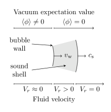
Figure 1: Cartoon showing features associated with the bubble wall. The scenario shown is a subsonic deflagration, where the wall speed $v_{\mathrm{w}}$ is slower than the speed of sound $c_{\mathrm{s}}$. The scalar field bubble wall is shown, while the ‘sound shell’ of nonzero fluid velocity in front of the wall is shaded. Above the diagram the value of $\langle\phi\rangle$ is shown, while below the radial fluid velocity $V_{r}$ is shown.

2 The electroweak phase transition

As discussed in the Introduction, without additional fields, the electroweak phase transition is a crossover in the Standard Model, occurring at a critical temperature of $159.5\pm 1.5\,\mathrm{GeV}$ [10].

However, adding just a single extra scalar field – real or complex; whether a singlet [11, 12, 13, 14, 15, 16], a second Higgs doublet [17, 18, 19, 20] or indeed a triplet (adjoint) Higgs field [21, 22], reopens the possibility of a first-order phase transition at the electroweak scale. Furthermore, these models all (to varying degrees) have regions of parameter space that will not be excluded in the near future by collider experiments [23].

There are therefore two motivations to study gravitational wave production from an electroweak phase transition.

First, and most importantly, it remains a well-motivated and attractive possibility to produce the observed baryon asymmetry through baryogenesis [24, 25] (see Ref. [26] for a review). Electroweak baryogenesis fulfils the Sakharov conditions [27] in the following manner:

1. $C$ and $CP$ violation: this occurs due to particles scattering off the bubble walls, producing asymmetries in front of the walls.

2. Baryon number $B$ violation: The $C$ and $CP$ violation means that sphaleron transitions in front of the wall are biased to produce more baryons than antibaryons.

3. Out of equilibrium: The bubble walls (and associated sound shells) disturb the symmetric-phase equilibrium state.

Even though the Standard Model is a crossover, and hence does not depart far from equilibrium, it is possible to achieve these requirements in the extensions mentioned above.

Second, a first-order phase transition at the electroweak scale would source gravitational waves that are potentially detectable by LISA [2] (see Refs. [28, 29], and also parts of Ref. [30] for other reviews). This would give a complementary probe of the particle physics at this energy scale, which will be studied extensively at planned experiments such as the Future Circular Collider [23, 31].

However, these two motivations are somewhat in tension. The energy density in gravitational waves produced by a phase transition is generally an increasing function of the wall velocity $v_{\mathrm{w}}$, so faster wall speeds are desirable. However, the process of electroweak baryogenesis outlined above depends on the wall velocity relative to the plasma in front of the wall being slower than the speed of sound [32], usually very much slower to allow particles to diffuse from the bubble wall (where $C$ and $CP$ violation occur) back into the plasma (where biased sphaleron transitions occur) [33]. Other variants of electroweak baryogenesis which allow for a fast detonation have been proposed, for example due to symmetry restoration behind the bubble wall [34], but further investigations – and perhaps simulations – of such scenarios would be beneficial.

For the remainder of this review, then, we concentrate on the signal from gravitational waves for its own sake, rather than as a signature of a process which generated the baryon asymmetry in the early universe.

3 Motion of the bubble wall and the “energy budget”

As described above, a thermal first-order phase transition proceeds by the nucleation of bubbles of the scalar field $\phi$ which is driving the transition; this is typically the Higgs field, although in models with additional scalar fields this is not always the case. The bubble nucleation rate at temperature $T$ is given by

$$\Gamma(T)=A(T)e^{-S_{3}(T)/T}$$ (1)

where $S_{3}$ is the three-dimensional bounce solution and $A(T)$ a dynamical prefactor of order $T^{4}$ [35]. The inverse duration of the phase transition $\beta$ relative to the Hubble rate $H_{*}$ at the time of the transition is then

$$\frac{\beta}{H_{*}}=\left.\left[T\frac{\mathrm{d}}{\mathrm{d}T}\left(\frac{S_{3}(T)}{T}\right)\right]\right|_{T=T_{*}}$$ (2)

where $T_{*}$ is the transition temperature, which we will assume for simplicity is close to the nucleation temperature $T_{\mathrm{n}}$. We will also assume that the duration of the phase transition is short enough that expansion can be neglected (i.e. $\beta/H_{*}\gtrsim 1$). The typical bubble radius $R_{*}$ is [35]

$$R_{*}=(8\pi)^{\frac{1}{3}}\frac{v_{\mathrm{w}}}{\beta},$$ (3)

where $v_{\mathrm{w}}$ is the wall velocity. To a first approximation, $R_{*}$ sets the inverse wavenumber of the peak of the gravitational wave power spectrum from a thermal first-order phase transition.

The scalar field has stress-energy tensor

$$T_{\mu\nu}^{\phi}=\partial_{\mu}\phi\partial_{\nu}\phi-g_{\mu\nu}\left(\frac{1}{2}\partial_{\rho}\phi\partial^{\rho}\phi-V(\phi)\right)$$ (4)

where $V(\phi)$ is the classical potential.

We treat this $\phi$ as a background field which interacts with all the particle content of the theory: Higgs bosons, quarks, leptons and gauge fields. These form a plasma and, employing distribution functions $f_{i}(k)$ for each particle species $i$, one finds that the equation of motion for $\phi$ including the interactions with the plasma can be written as [36, 37, 38]

$$\square\phi+\frac{\partial V(\phi)}{\partial\phi}+\sum_{i}\frac{\mathrm{d}m_{i}^{2}}{\mathrm{d}\phi}\int\frac{\mathrm{d}^{3}k}{(2\pi)^{3}2E_{i}}f_{i}(k),$$ (5)

where $m_{i}$ is the effective mass of the $i$th particle species (including all gauge bosons, pseudo-Goldstone modes and fermions) and $E_{i}^{2}=k^{2}+m_{i}^{2}$ (see Refs. [39, 40] for discussions of this approach in extensions of the Standard Model).

As the nucleated bubbles of the scalar field expand, they interact with the plasma. This excites the plasma and creates a ‘sound shell’ around the wall of plasma moving with nonzero outward radial velocity. Generally, if the wall velocity is smaller than the speed of sound, then this shell precedes the scalar field wall and the process is termed a ‘deflagration’ by analogy with standard terms from combustion physics. Conversely, if the wall velocity is faster than the speed of sound, then the sound shell is a rarefaction wave trailing the bubble wall and the resulting process is a ‘detonation’.

One can rewrite the equation of motion for the scalar field

$$\square\phi+\frac{\partial V_{\text{eff}}(\phi,T)}{\partial\phi}=\mathcal{K}(\phi);\qquad\mathcal{K}(\phi)=-\sum_{i}\frac{\mathrm{d}m_{i}^{2}}{\mathrm{d}\phi}\int\frac{\mathrm{d}^{3}k}{(2\pi)^{3}2E_{i}}\delta f_{i}(k),$$ (6)

where $V_{\text{eff}}$ is the thermal effective potential, and $\delta f_{i}(p)$ is the deviation of the distribution function of the $i$th particle species from equilibrium.

Figure 2: Sketch of forces acting on bubble wall. The latent heat released during the phase transition drives the bubble outwards, while its interaction with the plasma of light particles creates friction. When the two forces are balanced, the wall ceases to accelerate.

Equation (6) is important, for two reasons - firstly, it underpins important simplifying approximations including the fluid approximation that we shall use extensively throughout this work; and secondly, it is readily apparent that the equation is nothing more than a relationship between the outward force exerted by the bubble wall on the particles $f_{i}(p)$, driven by latent heat, and the resulting friction exerted on the bubble wall (see Fig. 2). Nevertheless, the expression is difficult to work with directly and so further simplifying assumptions are usually made.

In particular, one often approximates the equilibrium distribution functions for all the particle species $f_{i}$ by a relativistic fluid $u^{\mu}$. The stress-energy tensor of such a fluid is

$$T_{\mu\nu}^{\text{fluid}}=\sum_{i}\int\frac{\mathrm{d}^{3}k}{(2\pi)^{3}E_{i}}k_{\mu}k_{\nu}f_{i}(k)=wu_{\mu}u_{\nu}-g_{\mu\nu}p$$ (7)

where $w=\epsilon+p$ is the enthalpy; $\epsilon$ is the energy density of the fluid, and $p$ is the pressure. Energy conservation requires that the energy removed from the field $\phi$ by the friction term $\mathcal{K}(\phi)$ is deposited in the fluid:

$$\partial^{\mu}T_{\mu\nu}=\partial^{\mu}T_{\mu\nu}^{\phi}+\partial^{\mu}T_{\mu\nu}^{\text{fluid}}=0.$$ (8)

Working in the fluid approximation, one can take a more qualitative form for $\mathcal{K}(\phi)$

$$\mathcal{K}(\phi)=\eta(\phi,v_{\mathrm{w}})u^{\mu}\partial_{\mu}\phi.$$ (9)

The form of $\eta(\phi,v_{\mathrm{w}})$ is often chosen by comparison with the Boltzmann equations for $f_{i}(k)$ [41, 38]. Two choices that have been used in numerical simulations are

$$\eta(\phi,v_{\mathrm{w}})=\text{const.}\quad\text{and}\quad\eta(\phi,v_{\mathrm{w}})=\tilde{\eta}\frac{\phi^{2}}{T},$$ (10)

where $\tilde{\eta}$ is a dimensionless constant. The exact choice of $\eta(\phi,v_{\mathrm{w}})$ may slightly change the profile of the scalar field and fluid at the bubble wall. However, as these are at microscopic length scales when the phase transition occurs there is in practice little difference. Furthermore, $\phi$ tends to a constant and hence $\mathcal{K}(\phi)\to 0$ away from the bubble wall. We therefore expect that the fluid sound shell reaches a scaling profile parametrised by the dimensionless ratio $\xi=r/t$ and hence at collision has a size proportional to $R_{*}$.

For the purposes of the gravitational wave power spectrum, then, the scaling form of the radial fluid profile $V_{r}(\xi)[\equiv u_{r}/\gamma]$ and the wall velocity $v_{w}$ are all that matter. To know $V_{r}(\xi)$, one needs to know how much of the latent heat ends up as fluid kinetic energy.

We first define the phase transition strength $\alpha$ as the ratio of latent heat to radiation density at the time of transition in the symmetric phase

$$\alpha_{T}\equiv\frac{\mathcal{L}(T)}{g_{*}\pi^{2}T^{4}/30},$$ (11)

where $\mathcal{L}(T)$ is the latent heat and $g_{*}$ the number of relativistic degrees of freedom at temperature $T$. Note, however, that another definition of $\alpha$ based on the trace anomaly difference is sometimes used.

The fluid efficiency $\kappa_{\text{f}}$ then gives the fraction of this vacuum energy that is turned into kinetic energy in the plasma during the transition. It is approximately [42]

$$\kappa_{\mathrm{f}}(\alpha)\simeq\begin{cases}\dfrac{\alpha}{0.73+0.083\sqrt{\alpha}+\alpha},&v_{\mathrm{w}}\sim 1\\[15.0pt] \dfrac{v_{\mathrm{w}}^{6/5}6.9\alpha}{1.36-0.037\sqrt{\alpha}+\alpha},&v_{\mathrm{w}}\lesssim 0.1;\end{cases}$$ (12)

alternatively, if one knows the fluid velocity as a function of $\xi$ for a given scenario, the following expression can be used

$$\kappa_{\text{f}}=\frac{3}{\epsilon v_{\mathrm{w}}^{3}}\int\mathrm{d}\xi\,w(\xi)V_{r}^{2}\gamma^{2}\xi^{2}.$$ (13)

This expression has been used to produce the results shown in Fig. 3. The steady-state fluid equations of motion can be solved to give the full profile for $V_{r}(\xi)$ [42], or it can be found from simulations (see below).

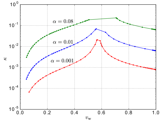
Figure 3: Efficiency $\kappa_{\mathrm{f}}$ measured (at points marked by circles) from spherically symmetric simulations of the field-fluid system for a single bubble by means of Eq. (13) (Cutting 2017, private communication). There is agreement with the analytically computed efficiency curves and in Ref. [42], even though the authors of that work used a bag model rather than the Standard Model-like effective potential employed here.

For a given $\alpha_{T_{*}}$ and $v_{\mathrm{w}}$, there is essentially no dependence on the microscopic details of the phase transition in computing $\kappa_{\mathrm{f}}$, and there are relatively few parameters required to adequately describe the physics of a thermal phase transition: the inverse phase transition duration $\beta/H_{*}$, the phase transition strength $\alpha_{T_{*}}$, and the wall velocity $v_{\mathrm{w}}$.

In the following section we show how these parameters can be used to compute the gravitational wave power spectrum.

4 Simulations, models and approximations

The first discussion of gravitational waves from a first-order electroweak phase transition already anticipated a substantial acoustic source [43]. Later works focused more on the collision of the bubbles themselves [44, 45, 46, 47], and the ‘envelope approximation’ – infinitestimally thin walls that disappear instantaneously when bubbles overlap – gained wide adoption. High-precision studies were then carried out [48].

Later it was observed that the fluid profiles are not infinitesimally thin – thus violating one requirement of the envelope approximation – and they do not disappear immediately after the bubbles have collided, leading instead to an acoustic regime. Some numerical work has also studied scalar field bubble collisions [44, 49], also as a comparison to the envelope approximation [50]. However, it remains that the envelope approximation and full realtime simulations with the field-fluid model have been of the greatest interest. We discuss their application to a general thermal phase transition below.

4.1 Envelope approximation

The envelope approximation has been widely used in the past to model gravitational wave power spectra from bubble collisions. It is really two approximations: that the stress-energy tensor of the expanding bubble is only nonzero in an infinitesimally thin shell on the bubble’s surface; and that this stress-energy disappears immediately when two bubbles intersect, hence only the ‘envelopes’ of the bubbles interact (see Fig. 4).

Figure 4: Sketch of a slice through a ‘simulation’ in the envelope approximation, with a spherical simulation volume. Only the uncollided portions of the thin bubble walls are recorded; there are no dynamics around the bubbles, or in the aftermath of bubble collisions.

These two simplifying assumptions lead to a very simple power spectrum – a rising $f^{3}$ power law for frequencies much smaller than the reciprocal bubble radius $1/R_{*}$, and a falling $f^{-1}$ for $f\gg 1/R_{*}$. This form has been confirmed by lattice simulations of colliding scalar field walls [50], as well as analytical modelling of coherent sums of infinitesimal fragments of bubble wall [51].

In Ref. [48], extensive studies of the form of the gravitational wave power spectrum in the envelope approximation were carried out. Based on their results, the authors postulated an ansatz of the broken power-law form

$$\Omega_{\text{GW}}(f)=\tilde{\Omega}_{\text{GW}}\frac{(a+b)\tilde{f}^{b}f^{a}}{b\tilde{f}^{(a+b)}+af^{(a+b)}}$$ (14)

where the power-law indices were (for fast walls) $a\approx 2.8$, $b\approx 1.0$, $\tilde{f}$ is the peak frequency [a more complicated function of function of $\beta$ and $v_{\mathrm{w}}$ than the inverse of Eq. (3)], and the amplitude $\tilde{\Omega}_{\text{GW}}$ scales roughly as the cube of $v_{\mathrm{w}}$.

In the past, the envelope approximation has been applied to all forms of bubble collision, with the efficiency factor $\kappa$ taken to refer to the efficiency of conversion of latent heat into fluid kinetic energy, namely $\kappa_{\mathrm{f}}$. However, since the fluid shells associated with the growing bubbles scale with the bubble radius, it is not necessarily appropriate to make the approximation that the bubble walls are infinitesimally thin. Furthermore, the envelope approximation does not attempt to handle the aftermath of bubble collisions.

For these reasons, the envelope approximation is best used for modelling the scalar field contribution to first-order phase transitions (which is only significant in certain circumstances), and more sophisticated simulation and modelling techniques are required.

4.2 The field-fluid model

Motivated by the fluid approximation discussed in the previous section, it is natural to consider both analytical and numerical studies of the coupled field-fluid model. The equations of motion are

$$(\partial_{\mu}\partial^{\mu}\phi)\partial^{\nu}\phi-\frac{\partial V_{\text{eff}}(\phi,T)}{\partial\phi}\partial^{\nu}\phi =+\eta(\phi,v_{\mathrm{w}})u^{\mu}\partial_{\mu}\phi\partial^{\nu}\phi$$ (15)

$$\partial_{\mu}(wu^{\mu}u^{\nu})-\partial^{\nu}p+\frac{\partial V_{\text{eff}}(\phi,T)}{\partial\phi}\partial^{\nu}\phi =-\eta(\phi,v_{\mathrm{w}})u^{\mu}\partial_{\mu}\phi\partial^{\nu}\phi.$$ (16)

In a realtime numerical simulation of the system, the scalar field is typically evolved using a standard leapfrog algorithm, while standard operator-splitting grid-based techniques for the relativistic fluid are required (see e.g. Ref. [52]).

The microscopic physics of the sound shell, and the resulting gravitational wave power spectrum, does not depend on the detailed physics of the bubble wall. In simulations it is therefore usually sufficient to consider a simplified effective potential $V_{\text{eff}}(\phi,T)$ which yields the correct latent heat $\mathcal{L}$.

It is relatively straightforward to solve the system of hydrodynamic equations to find the scalar field and fluid velocity profile around the bubble wall [47, 42, 41], or else one can evolve the above system of equations until a steady state is reached.

When carrying out a full three-dimensional numerical simulation of the system both the scalar field and the fluid source gravitational waves, through the relevant transverse-traceless spatial parts of their stress energy tensors,

$$\tau^{\phi}_{ij}=\partial_{i}\phi\partial_{j}\phi;\qquad\tau^{\mathrm{f}}_{ij}=wu_{i}u_{j}.$$ (17)

The largest three-dimensional lattice simulations of the system performed to date use lattices with side lengths of $4200$ sites. The smallest physically resolvable scales are of the order of the spacing between sites, while the largest are comparable to the size of the lattice itself. This means that there can only be at most two or three orders of magnitude between the bubble wall thickness and the bubble radius. Hence the gravitational wave power sourced by $\tau_{ij}^{\phi}$ will be orders of magnitude larger than it should be, relative to that sourced by $\tau_{ij}^{\mathrm{f}}$. When extrapolating from the results of numerical simulations, then, $\tau_{ij}^{\phi}$ is not included as a source of gravitational waves.

For further details about simulating the system of equations (15-16), see Refs. [53, 54, 55] (spherically symmetric simulations) and Refs. [56, 57, 58, 59] (in three separate spatial dimensions). Portions of a slice through some of the latest three-dimensional simulations are shown in Fig. 5.

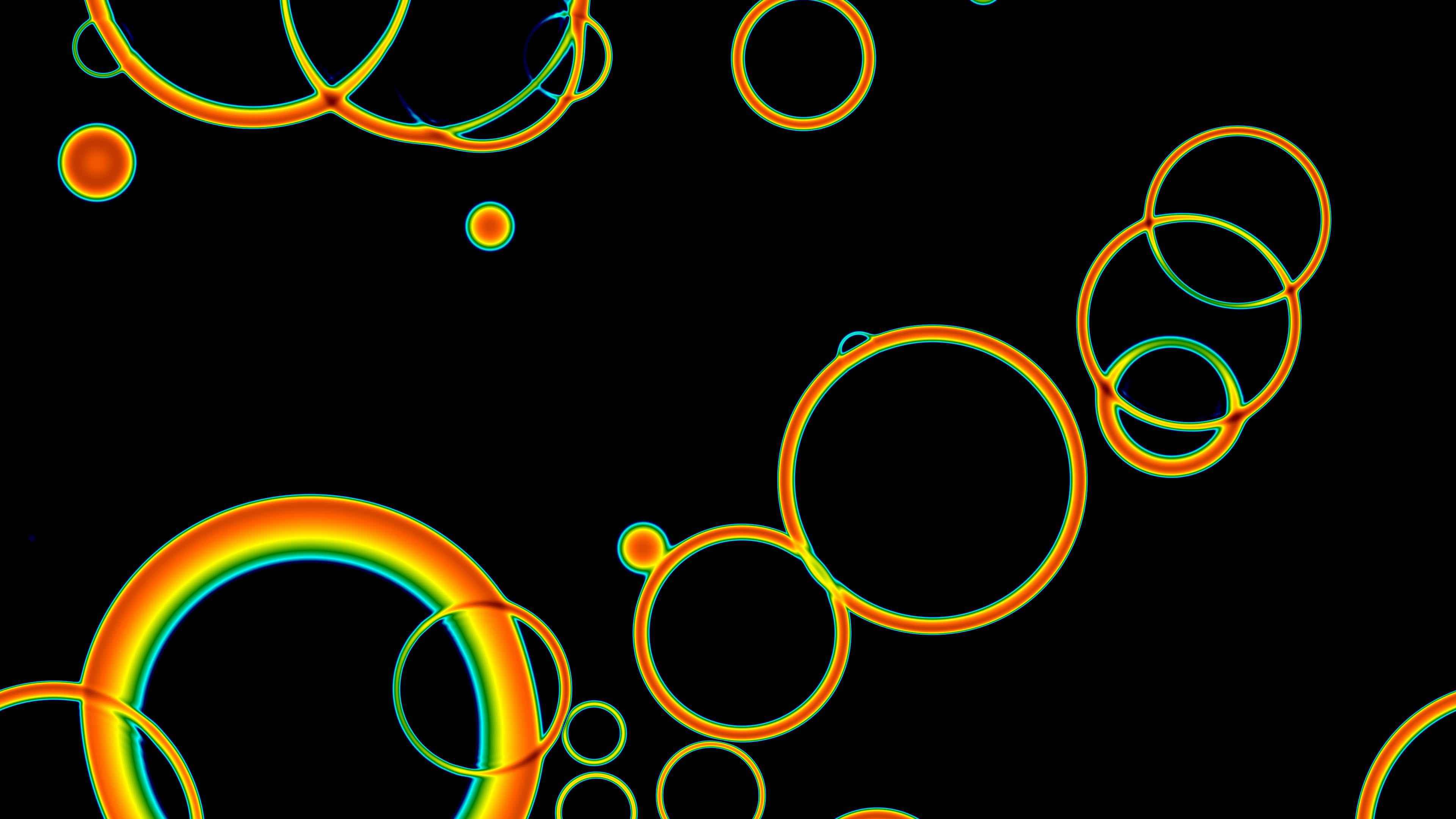
Figure 5: Portions of slices through a three-dimensional field-fluid simulation, with hotter colours indicating relatively higher fluid kinetic energies. Here $\alpha_{T_{*}}\approx 0.01$ and $v_{\mathrm{w}}\approx 0.68$. The slice at left shows mostly uncollided bubbles, while the slice at right is from long after the bubbles have collided.

5 Gravitational wave production processes

Based on the simulation results described in the previous section and additional analytical calculations and modelling, we can now present some ansätze for the resulting gravitational wave power spectrum. We follow the discussion in Ref. [2], updated to incorporate recent results [59].

The production of gravitational waves at a first-order phase transition can be separated into three stages.

• The first is the initial collision of the scalar field shells, which is of limited duration and generally subdominant unless the fluid efficiency is low or the system undergoes a vacuum transition in the absence of a thermal plasma. The gravitational wave power spectrum sourced by this stage is often denoted $\Omega_{\text{env}}$.

• After the bubbles have merged, the wave of fluid kinetic energy in the plasma continues to propagate outwards into the broken phase. Without the driving force of the scalar field bubble wall, these waves travel at the speed of sound in the plasma. As the shells of kinetic energy from different bubbles overlap, gravitational waves are produced. The power spectrum produced by this source is denoted $\Omega_{\text{sw}}$.

• Finally the acoustic phase may give way to shocks [60] and a turbulent regime [47, 61, 62, 63, 64]. The power spectrum is expected from analytical calculations to be rather different in this regime, but no simulations have yet captured time- and length-scales adequate to probe the onset of turbulence. We denote the resulting power spectrum $\Omega_{\text{turb}}$.

Peaking at different length scales, and on different time scales, the three sources are expected to approximately sum together

$$\Omega_{\text{GW}}=\Omega_{\text{env}}+\Omega_{\text{sw}}+\Omega_{\text{turb}}.$$ (18)

Each source will contribute to a different extent, depending on the exact details of the phase transition in question. For simplicity we assume that the bubble wall does not run away, nor that it is carefully tuned to produce a hybrid profile (with a wall velocity close to the Chapman-Jouguet velocity).

For the remainder of this section we summarise the form of these three power spectra, motivated by simulations and analytic work. We will consider ansätze for the amplitude of each of these sources at the present day. For further information see Ref. [2].

5.1 Colliding scalar field shells

For the collision of scalar field shells the best available results are those obtained from Refs. [48, 51]. Based on the latter, we write the gravitational wave power spectrum as

$$h^{2}\Omega_{\text{env}}(f)=1.67\times 10^{-5}\,\Delta\left(\frac{H_{*}}{\beta}\right)^{2}\left(\frac{\kappa_{\phi}\alpha_{T_{*}}}{1+\alpha_{T_{*}}}\right)^{2}\left(\frac{100}{g_{*}}\right)^{\frac{1}{3}}S_{\text{env}}(f)$$ (19)

with the spectral form (for $v_{\mathrm{w}}$ close to 1)

$$S_{\text{env}}(f)=\left[c_{l}\left(\frac{f}{f_{\text{env}}}\right)^{-3}+(1-c_{l}-c_{h})\left(\frac{f}{f_{\text{env}}}\right)^{-1}+c_{h}\left(\frac{f}{f_{\text{env}}}\right)\right]^{-1}$$ (20)

where fitting yields $c_{l}=0.064$ and $c_{h}=0.48$ and the power law indices are fixed. The peak frequency is

$$f_{\text{env}}=16.5\,\mu\mathrm{Hz}\,\left(\frac{f_{*}}{\beta}\right)\left(\frac{\beta}{H_{*}}\right)\left(\frac{T_{*}}{100\,\mathrm{GeV}}\right)\left(\frac{g_{*}}{100}\right)^{\frac{1}{6}}.$$ (21)

The dependence of the amplitude and peak frequency on $v_{\mathrm{w}}$ is

$$\Delta=\frac{0.48v_{\mathrm{w}}^{3}}{1+5.3v_{\mathrm{w}}^{2}+5v_{\mathrm{w}}^{4}};\quad\frac{f_{*}}{\beta}=\frac{0.35}{1+0.069v_{\mathrm{w}}+0.69v_{\mathrm{w}}^{4}}.$$ (22)

Into Eqs. (19) and (21), one inserts the transition temperature $T_{*}$, phase transition strength $\alpha_{T_{*}}$, wall velocity $v_{\mathrm{w}}$ and nucleation rate relative to the Hubble rate, $H_{*}/\beta$. Furthermore, the ‘efficiency’ factor $\kappa_{\phi}$ of converting vacuum energy into scalar field gradient energy is required. This naturally depends on both the surface tension and the surface area of bubbles at collision. However, it is not straightforward to calculate the surface area, which depends in a nontrivial way on the nucleation rate [50]. A very crude approximation would be

$$\kappa_{\phi}\sim\frac{\gamma\sigma}{R_{*}\rho_{\text{vac}}},$$ (23)

where $\gamma$ is the relativistic gamma associated with the wall velocity, $\sigma$ is the surface tension, and $\rho_{\text{vac}}$ the vacuum energy density. A more refined approach could be to use the expression for the symmetric phase volume in Ref. [35] to infer the total surface area. For general thermal phase transitions, which are the focus of this work, we would expect $\kappa_{\phi}$ to be vanishingly small: as the walls reach their terminal velocity, $\gamma$ approaches a constant, and so the overall expression scales with $1/R_{*}$.

On the other hand, for runaway and vacuum transitions essentially all of the vacuum energy goes into accelerating the bubble walls to relativistic speeds. The efficiency factor $\kappa_{\phi}$ must then be close to unity, and the gravitational waves are then principally sourced by the scalar field gradient energy.

5.2 Acoustic waves

For a general thermal phase transition, the initial collisional phase is short-lived; furthermore, the scalar field gradient energy scales only as the surface area of the bubbles rather than the volume. A more significant, and long-lasting source of gravitational waves is produced by expanding sound shells in the fluid kinetic energy after the bubbles have collided.

In fact, for non-ultrarelativistic fluid flows, it is straightforward to obtain the gravitational wave power spectrum from acoustic waves through a convolution of the fluid velocity power [65], and, in turn, this can be derived from a fluid profile obtained through the methods discussed earlier [66]. However, there is incomplete agreement with the fluid velocity power spectrum observed in simulations, perhaps due to the analytical work of Ref. [66] not modelling the initial collisions of the fluid profiles. We therefore concentrate for the time being on results derived from recent very-large scale simulations [59].

The following ansatz for the gravitational wave power spectrum from acoustic waves was first put forward in Ref. [2] and in Ref. [59] was found to generally agree with simulation results. The version presented here is based on the latter work:

$$h^{2}\Omega_{\text{sw}}(f)=8.5\times 10^{-6}\left(\frac{100}{g_{*}}\right)^{\frac{1}{3}}\Gamma^{2}\overline{U}_{\mathrm{f}}^{4}\left(\frac{H_{*}}{\beta}\right)v_{\mathrm{w}}\,S_{\text{sw}}(f)$$ (24)

where the adiabatic index $\Gamma=\overline{w}/\overline{\epsilon}\approx 4/3$; $\overline{w}$ and $\overline{\epsilon}$ are the volume-averaged enthalpy and energy density respectively. The quantity $\overline{U}_{\mathrm{f}}$ is a measure of the rms fluid velocity

$$\overline{U}_{\mathrm{f}}^{2}=\frac{1}{\overline{w}}\frac{1}{\mathcal{V}}\int_{\mathcal{V}}\mathrm{d}^{3}x\,\tau_{ii}^{\mathrm{f}}\approx\frac{3}{4}\kappa_{\mathrm{f}}\alpha_{T_{*}}$$ (25)

where the integral and average is over a volume $\mathcal{V}$. The spectral shape is

$$S_{\text{sw}}(f)=\left(\frac{f}{f_{\mathrm{sw}}}\right)^{3}\left(\frac{7}{4+3(f/f_{\mathrm{sw}})^{2}}\right)^{7/2}$$ (26)

with approximate peak frequency

$$f_{\mathrm{sw}}=8.9\,\mu\mathrm{Hz}\,\frac{1}{v_{\mathrm{w}}}\left(\frac{\beta}{H_{*}}\right)\left(\frac{z_{\mathrm{p}}}{10}\right)\left(\frac{T_{*}}{100\,\mathrm{GeV}}\right)\left(\frac{g_{*}}{100}\right)^{\frac{1}{6}}$$ (27)

with $z_{\mathrm{p}}$ a simulation-derived factor that is usually around 10, but may be higher when $v_{\mathrm{w}}\approx c_{\mathrm{s}}$ [59].

We finish this section by making a comment on the timescale on which shocks and then turbulence would appear [67, 60]. It is given by the ratio

$$\tau_{\text{sh}}\sim\mathrm{L}_{f}/\overline{U}_{\mathrm{f}},$$ (28)

where $\mathrm{L_{\mathrm{f}}}$ is a measure of the characteristic length scale associated with fluid flows – to first approximation this is the physical bubble radius $R_{*}$. Thus when the ratio $H_{*}R_{*}/\overline{U}_{\mathrm{f}}\ll 1$, shocks can develop within a Hubble time and the onset of turbulence must be taken into consideration.

5.3 Turbulence

Until simulations are available of the onset of turbulence, we must make do with analytical results. From modelling of Kolmogorov-type turbulence [63], one obtains [2]

$$h^{2}\Omega_{\text{turb}}(f)=3.35\times 10^{-4}\left(\frac{H_{*}}{\beta}\right)\left(\frac{\kappa_{\text{turb}}\alpha_{T_{*}}}{1+\alpha_{T_{*}}}\right)^{\frac{3}{2}}\left(\frac{100}{g_{*}}\right)^{\frac{1}{3}}v_{\mathrm{w}}S_{\text{turb}}(f).$$ (29)

Here the quantity $\kappa_{\text{turb}}$ is the efficiency of conversion of latent heat into turbulent flows. Based on simulation results so far, at most a few percent of the fluid kinetic energy is converted into rotational flow, so we might expect $\kappa_{\text{turb}}$ to be negligible. However, we have not yet been able to study the timescale of shock appearance [Eq. (28)] in simulations, so it remains likely that turbulent flows do form in many scenarios.

Although the amplitude is uncertain, the spectral shape of the turbulent contribution is known exactly [63]

$$S_{\text{turb}}(f)=\frac{(f/f_{\text{turb}})^{3}}{[1+(f/f_{\text{turb}})]^{\frac{11}{3}}(1+8\pi f/h_{*})}$$ (30)

where $h_{*}$ is the Hubble rate at $T_{*}$,

$$h_{*}=16.5\,\mu\mathrm{Hz}\left(\frac{T_{*}}{100\,\mathrm{GeV}}\right)\left(\frac{g_{*}}{100}\right)^{\frac{1}{6}}.$$ (31)

The peak frequency $f_{\text{turb}}$ is slightly higher than for the sound wave contribution,

$$f_{\text{turb}}=27\,\mu\mathrm{Hz}\,\frac{1}{v_{\mathrm{w}}}\left(\frac{\beta}{H_{*}}\right)\left(\frac{T_{*}}{100\,\mathrm{GeV}}\right)\left(\frac{g_{*}}{100}\right)^{\frac{1}{6}}.$$ (32)

6 From models to power spectra

We have now discussed the means by which the three contributions to the gravitational wave power spectrum can be studied analytically, simulated and modelled.

In Fig. 6, we plot the gravitational wave power spectrum based on the ansätze of the previous section, for a deflagration with $v_{\mathrm{w}}=0.44$, $\alpha_{T_{*}}=0.084$, taking the Standard Model value $g_{*}=106.75$. Using the corresponding simulation result from Ref. [59], we find that $z_{\mathrm{p}}=6.9$, $\overline{U}_{\mathrm{f}}=0.055$ and $\Gamma\approx 4/3$. To turn these phase transition results into a possible scenario, we use a transition temperature $T_{*}=180\,\mathrm{GeV}$ and take $H_{*}/\beta=0.1$ (for which shocks are unlikely to develop before Hubble expansion attenuates the signal).

We compare this example power spectrum with the sensitivity curve for power laws (see Ref. [68]) for the eLISA configuration closest to that proposed for LISA: 6 laser links, arm length of $2~{}\mathrm{Gm}$ and mission duration of 5 years. In the example given, the signal-to-noise ratio (SNR) should mean that detection of such a scenario is possible. Nevertheless a careful evaluation of the SNR is required [68, 2].

To study the gravitational waves power spectrum resulting from a specific extension of the Standard Model, one needs to supply at least $\alpha_{T_{*}}$, $\beta$, $T_{*}$, and $v_{\mathrm{w}}$. This has been done, for example, for the real singlet model in Refs. [14, 15].

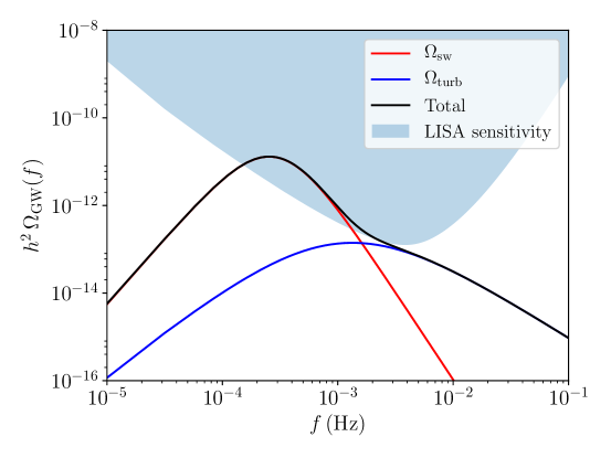
Figure 6: Example of the gravitational wave power spectrum for a thermal phase transition, using the ansätze given in the text and with $v_{\mathrm{w}}=0.44$, $\alpha_{T_{*}}=0.084$, $H_{*}/\beta=0.1$ and $T_{*}=180\,\mathrm{GeV}$ (see Section 6). The power spectrum is compared to a sensitivity curve obtained for a LISA-like configuration.

7 Outlook

Gravitational waves produced by an electroweak phase transition are a realistic candidate for detection by future space-based gravitational wave detectors, such as LISA. The latest simulation and modelling results indicate that it is principally the acoustic source that is responsible for production of gravitational waves, although the role of turbulence still requires clarification. The interplay between the acoustic phase and the formation of shocks and turbulent behaviour is still poorly understood. Further simulations are likely to be required.

We are entering a period when the electroweak phase transition will come under increasing scrutiny, in preparation for future colliders, as well as for the detectability of gravitational waves. Precision results for thermodynamic quantities in a wide variety of models are required, possibly from simulations of dimensionally reduced models (see e.g. [69] for the real singlet case). These yield the phase diagram and hence $T_{*}$, but in addition, the latent heat [70] (and hence $\alpha_{T_{*}}$) as well as the nucleation rate [71] (and hence $\beta$) can be determined. Combining these simulation results could yield a computation of the gravitational wave power spectrum based almost entirely on nonperturbative results. However, other techniques will still be required to determine $v_{\mathrm{w}}$.

Throughout this paper we have specialised to the case of a bubble wall where a terminal wall velocity $v_{\mathrm{w}}<1$ is reached, rather than a vacuum or runaway transition. Vacuum transitions have not been studied extensively on the lattice. It is to be expected that the envelope approximation performs well in these cases, however this remains to be confirmed in future work.

Runaway transitions change the analysis slightly as they do not stir up as much fluid kinetic energy, so the role of the colliding scalar field bubble walls is likely to be more significant. However, since higher-order corrections prevent true runaway transitions from occurring [7], the analysis in this review should be sufficient.

Competing Interests. The author declares that they have no competing interests.

Funding I acknowledge PRACE for awarding me access to resource HAZEL HEN based in Germany at the High Performance Computing Center Stuttgart (HLRS). This work is supported by the Academy of Finland grant 286769.

Acknowledgments I acknowledge useful discussions with Mark Hindmarsh and Kari Rummukainen. I am grateful to Daniel Cutting for supplying Fig. 3.

Erratum

Issues with the sound wave power spectrum formula

Equation (24) based on Ref. [59] unfortunately includes a number of errors. Firstly, in Ref. [59], the equivalent equation in the main body of the paper, Eq. (45), appears without the reduced Hubble constant squared $h^{2}$ on the left hand side, where the present-day Hubble constant is defined as $H_{0}=h\times 100\,\mathrm{km}\;\mathrm{s}^{-1}\;\mathrm{Mpc}^{-1}$.

The remainder of the issues are corrected in the Erratum of Ref. [59]:

• There was a factor of 3 missing from the right hand side of Eq. (39), which yields a factor 3 in Eq. (45).

• The numerical coefficient in Eq. (45) should have been 0.687, not 0.68.

• The value quoted for $\tilde{\Omega}_{\text{gw}}$ in the main body was an order of magnitude too large and should be $\tilde{\Omega}_{\text{gw}}=1.2\times 10^{-2}$.

Incorporating these changes, and multiplying both sides by $h^{2}$, with the contemporaneous Planck best-fit value $h=0.678$ (also used in Ref. [59]), we arrive at the following replacement formula for this paper’s Eq. (24):

$$h^{2}\Omega_{\text{sw}}(f)=1.19\times 10^{-6}\left(\frac{100}{g_{*}}\right)^{\frac{1}{3}}\Gamma^{2}\overline{U}_{\mathrm{f}}^{4}\left(\frac{H_{*}}{\beta}\right)v_{\mathrm{w}}\,S_{\text{sw}}(f),$$ (33)

noting that $R_{*}=(8\pi)^{\frac{1}{3}}v_{\mathrm{w}}/\beta$ as in Eq. (3). The gravitational wave power spectrum shown in Fig. 6 is also therefore incorrect. An updated plot is, however, not included here for several reasons: our understanding of turbulence after a phase transition has improved since this paper came out; the expected LISA sensitivity curve has changed; and foregrounds are neglected.

As source modeling has improved since this paper was originally published, the interested reader is encouraged to compare the formulae in this paper with more recent results.

I apologise for any confusion caused.

Acknowledgments I am grateful to Jenni Häkkinen for a careful comparison of the sound wave power spectrum expressions found across the literature. I also acknowledge Pasquale Di Bari for pointing out that this review paper reproduced mistakes found in Ref. [59], as well as introducing some more.

References

- Audley et al. [2017] H. Audley et al., (2017), arXiv:1702.00786 [astro-ph.IM] .
- Caprini et al. [2016] C. Caprini et al., JCAP 1604, 001 (2016), arXiv:1512.06239 [astro-ph.CO] .
- Kajantie et al. [1996a] K. Kajantie, M. Laine, K. Rummukainen, and M. E. Shaposhnikov, Phys. Rev. Lett. 77, 2887 (1996a), arXiv:hep-ph/9605288 [hep-ph] .
- Gurtler et al. [1997] M. Gurtler, E.-M. Ilgenfritz, and A. Schiller, Phys.Rev. D56, 3888 (1997), arXiv:hep-lat/9704013 [hep-lat] .
- Csikor et al. [1999] F. Csikor, Z. Fodor, and J. Heitger, Phys.Rev.Lett. 82, 21 (1999), arXiv:hep-ph/9809291 [hep-ph] .
- Bodeker and Moore [2009] D. Bodeker and G. D. Moore, JCAP 0905, 009 (2009), arXiv:0903.4099 [hep-ph] .
- Bodeker and Moore [2017] D. Bodeker and G. D. Moore, JCAP 1705, 025 (2017), arXiv:1703.08215 [hep-ph] .
- Dev and Mazumdar [2016] P. S. B. Dev and A. Mazumdar, Phys. Rev. D93, 104001 (2016), arXiv:1602.04203 [hep-ph] .
- Garcia Garcia et al. [2018] I. Garcia Garcia, S. Krippendorf, and J. March-Russell, Phys. Lett. B 779, 348 (2018), arXiv:1607.06813 [hep-ph] .
- D’Onofrio and Rummukainen [2016] M. D’Onofrio and K. Rummukainen, Phys. Rev. D93, 025003 (2016), arXiv:1508.07161 [hep-ph] .
- Barger et al. [2008] V. Barger, P. Langacker, M. McCaskey, M. J. Ramsey-Musolf, and G. Shaughnessy, Phys. Rev. D77, 035005 (2008), arXiv:0706.4311 [hep-ph] .
- Profumo et al. [2007] S. Profumo, M. J. Ramsey-Musolf, and G. Shaughnessy, JHEP 08, 010 (2007), arXiv:0705.2425 [hep-ph] .
- Damgaard et al. [2016] P. H. Damgaard, A. Haarr, D. O’Connell, and A. Tranberg, JHEP 02, 107 (2016), arXiv:1512.01963 [hep-ph] .
- Vaskonen [2017] V. Vaskonen, Phys. Rev. D95, 123515 (2017), arXiv:1611.02073 [hep-ph] .
- Beniwal et al. [2017] A. Beniwal, M. Lewicki, J. D. Wells, M. White, and A. G. Williams, JHEP 08, 108 (2017), arXiv:1702.06124 [hep-ph] .
- Chen et al. [2017] C.-Y. Chen, J. Kozaczuk, and I. M. Lewis, JHEP 08, 096 (2017), arXiv:1704.05844 [hep-ph] .
- Cline and Lemieux [1997] J. M. Cline and P.-A. Lemieux, Phys. Rev. D55, 3873 (1997), arXiv:hep-ph/9609240 [hep-ph] .
- Fromme et al. [2006] L. Fromme, S. J. Huber, and M. Seniuch, JHEP 11, 038 (2006), arXiv:hep-ph/0605242 [hep-ph] .
- Dorsch et al. [2013] G. C. Dorsch, S. J. Huber, and J. M. No, JHEP 10, 029 (2013), arXiv:1305.6610 [hep-ph] .
- Haarr et al. [2016] A. Haarr, A. Kvellestad, and T. C. Petersen, (2016), arXiv:1611.05757 [hep-ph] .
- Gunion et al. [1990] J. F. Gunion, R. Vega, and J. Wudka, Phys. Rev. D42, 1673 (1990).
- Fileviez Perez et al. [2009] P. Fileviez Perez, H. H. Patel, M. Ramsey-Musolf, and K. Wang, Phys. Rev. D79, 055024 (2009), arXiv:0811.3957 [hep-ph] .
- Curtin et al. [2014] D. Curtin, P. Meade, and C.-T. Yu, JHEP 11, 127 (2014), arXiv:1409.0005 [hep-ph] .
- Kuzmin et al. [1985] V. A. Kuzmin, V. A. Rubakov, and M. E. Shaposhnikov, Phys. Lett. B155, 36 (1985).
- Shaposhnikov [1987] M. E. Shaposhnikov, Nucl. Phys. B287, 757 (1987).
- Morrissey and Ramsey-Musolf [2012] D. E. Morrissey and M. J. Ramsey-Musolf, New J. Phys. 14, 125003 (2012), arXiv:1206.2942 [hep-ph] .
- Sakharov [1967] A. D. Sakharov, Pisma Zh. Eksp. Teor. Fiz. 5, 32 (1967), [Usp. Fiz. Nauk161,61(1991)].
- Grojean and Servant [2007] C. Grojean and G. Servant, Phys. Rev. D75, 043507 (2007), arXiv:hep-ph/0607107 [hep-ph] .
- Leitao et al. [2012] L. Leitao, A. Megevand, and A. D. Sanchez, JCAP 1210, 024 (2012), arXiv:1205.3070 [astro-ph.CO] .
- Cai et al. [2017] R.-G. Cai, Z. Cao, Z.-K. Guo, S.-J. Wang, and T. Yang, Natl. Sci. Rev. 4, 687 (2017), arXiv:1703.00187 [gr-qc] .
- Contino et al. [2017] R. Contino et al., CERN Yellow Report , 255 (2017), arXiv:1606.09408 [hep-ph] .
- No [2011] J. M. No, Phys. Rev. D84, 124025 (2011), arXiv:1103.2159 [hep-ph] .
- Joyce et al. [1995] M. Joyce, T. Prokopec, and N. Turok, Phys. Rev. Lett. 75, 1695 (1995), [Erratum: Phys. Rev. Lett.75,3375(1995)], arXiv:hep-ph/9408339 [hep-ph] .
- Caprini and No [2012] C. Caprini and J. M. No, JCAP 1201, 031 (2012), arXiv:1111.1726 [hep-ph] .
- Enqvist et al. [1992] K. Enqvist, J. Ignatius, K. Kajantie, and K. Rummukainen, Phys. Rev. D45, 3415 (1992).
- Liu et al. [1992] B.-H. Liu, L. D. McLerran, and N. Turok, Phys. Rev. D46, 2668 (1992).
- Moore and Prokopec [1995] G. D. Moore and T. Prokopec, Phys. Rev. D52, 7182 (1995), arXiv:hep-ph/9506475 [hep-ph] .
- Konstandin et al. [2014] T. Konstandin, G. Nardini, and I. Rues, JCAP 1409, 028 (2014), arXiv:1407.3132 [hep-ph] .
- Megevand and Sanchez [2010] A. Megevand and A. D. Sanchez, Nucl. Phys. B825, 151 (2010), arXiv:0908.3663 [hep-ph] .
- Kozaczuk [2015] J. Kozaczuk, JHEP 10, 135 (2015), arXiv:1506.04741 [hep-ph] .
- Huber and Sopena [2013] S. J. Huber and M. Sopena, (2013), arXiv:1302.1044 [hep-ph] .
- Espinosa et al. [2010] J. R. Espinosa, T. Konstandin, J. M. No, and G. Servant, JCAP 1006, 028 (2010), arXiv:1004.4187 [hep-ph] .
- Hogan [1986] C. J. Hogan, Mon. Not. Roy. Astron. Soc. 218, 629 (1986).
- Kosowsky et al. [1992a] A. Kosowsky, M. S. Turner, and R. Watkins, Phys.Rev. D45, 4514 (1992a).
- Kosowsky et al. [1992b] A. Kosowsky, M. S. Turner, and R. Watkins, Phys.Rev.Lett. 69, 2026 (1992b).
- Kosowsky and Turner [1993] A. Kosowsky and M. S. Turner, Phys.Rev. D47, 4372 (1993), arXiv:astro-ph/9211004 [astro-ph] .
- Kamionkowski et al. [1994] M. Kamionkowski, A. Kosowsky, and M. S. Turner, Phys.Rev. D49, 2837 (1994), arXiv:astro-ph/9310044 [astro-ph] .
- Huber and Konstandin [2008] S. J. Huber and T. Konstandin, JCAP 0809, 022 (2008), arXiv:0806.1828 [hep-ph] .
- Child and Giblin [2012] H. L. Child and J. Giblin, John T., JCAP 1210, 001 (2012), arXiv:1207.6408 [astro-ph.CO] .
- Weir [2016] D. J. Weir, Phys. Rev. D93, 124037 (2016), arXiv:1604.08429 [astro-ph.CO] .
- Jinno and Takimoto [2017] R. Jinno and M. Takimoto, Phys. Rev. D95, 024009 (2017), arXiv:1605.01403 [astro-ph.CO] .
- Wilson and Matthews [2003] J. Wilson and G. Matthews, Relativistic Numerical Hydrodyamics (Cambridge University Press, Cambridge, 2003).
- Kurki-Suonio and Laine [1996a] H. Kurki-Suonio and M. Laine, Phys.Rev. D54, 7163 (1996a), arXiv:hep-ph/9512202 [hep-ph] .
- Kurki-Suonio and Laine [1996b] H. Kurki-Suonio and M. Laine, Phys.Rev.Lett. 77, 3951 (1996b), arXiv:hep-ph/9607382 [hep-ph] .
- Giblin and Mertens [2013] J. T. Giblin, Jr. and J. B. Mertens, JHEP 12, 042 (2013), arXiv:1310.2948 [hep-th] .
- Hindmarsh et al. [2014] M. Hindmarsh, S. J. Huber, K. Rummukainen, and D. J. Weir, Phys.Rev.Lett. 112, 041301 (2014), arXiv:1304.2433 [hep-ph] .
- Hindmarsh et al. [2015] M. Hindmarsh, S. J. Huber, K. Rummukainen, and D. J. Weir, Phys. Rev. D92, 123009 (2015), arXiv:1504.03291 [astro-ph.CO] .
- Giblin and Mertens [2014] J. T. Giblin and J. B. Mertens, Phys.Rev. D90, 023532 (2014), arXiv:1405.4005 [astro-ph.CO] .
- Hindmarsh et al. [2017] M. Hindmarsh, S. J. Huber, K. Rummukainen, and D. J. Weir, Phys. Rev. D 96, 103520 (2017), [Erratum: Phys.Rev.D 101, 089902 (2020)], arXiv:1704.05871 [astro-ph.CO] .
- Pen and Turok [2016] U.-L. Pen and N. Turok, Phys. Rev. Lett. 117, 131301 (2016), arXiv:1510.02985 [astro-ph.CO] .
- Kosowsky et al. [2002] A. Kosowsky, A. Mack, and T. Kahniashvili, Phys.Rev. D66, 024030 (2002), arXiv:astro-ph/0111483 [astro-ph] .
- Nicolis [2004] A. Nicolis, Class.Quant.Grav. 21, L27 (2004), arXiv:gr-qc/0303084 [gr-qc] .
- Caprini et al. [2009] C. Caprini, R. Durrer, and G. Servant, JCAP 0912, 024 (2009), arXiv:0909.0622 [astro-ph.CO] .
- Kahniashvili et al. [2012] T. Kahniashvili, A. Brandenburg, L. Campanelli, B. Ratra, and A. G. Tevzadze, Phys. Rev. D86, 103005 (2012), arXiv:1206.2428 [astro-ph.CO] .
- Caprini and Durrer [2006] C. Caprini and R. Durrer, Phys.Rev. D74, 063521 (2006), arXiv:astro-ph/0603476 [astro-ph] .
- Hindmarsh [2018] M. Hindmarsh, Phys. Rev. Lett. 120, 071301 (2018), arXiv:1608.04735 [astro-ph.CO] .
- Landau and Lifshitz [1987] L. D. Landau and E. M. Lifshitz, Fluid Mechanics, 2nd ed., Course of Theoretical Physics, Vol. 6 (Butterworth-Heinemann, 1987).
- Thrane and Romano [2013] E. Thrane and J. D. Romano, Phys. Rev. D88, 124032 (2013), arXiv:1310.5300 [astro-ph.IM] .
- Brauner et al. [2017] T. Brauner, T. V. I. Tenkanen, A. Tranberg, A. Vuorinen, and D. J. Weir, JHEP 03, 007 (2017), arXiv:1609.06230 [hep-ph] .
- Kajantie et al. [1996b] K. Kajantie, M. Laine, K. Rummukainen, and M. E. Shaposhnikov, Nucl. Phys. B466, 189 (1996b), arXiv:hep-lat/9510020 [hep-lat] .
- Moore and Rummukainen [2001] G. D. Moore and K. Rummukainen, Phys. Rev. D63, 045002 (2001), arXiv:hep-ph/0009132 [hep-ph] .