The Globular Cluster – Dark Matter Halo Connection

Abstract

I present a simple phenomenological model for the observed linear scaling of the stellar mass in old globular clusters (GCs) with $z=0$ halo mass in which the stellar mass in GCs scales linearly with progenitor halo mass at $z=6$ above a minimum halo mass for GC formation. This model reproduces the observed $M_{\rm GCs}-M_{\rm halo}$ relation at $z=0$ and results in a prediction for the minimum halo mass at $z=6$ required for hosting one GC: $M_{\rm min}(z=6)=1.07\times 10^{9}\,M_{\odot}$. Translated to $z=0$, the mean threshold mass is $M_{\rm halo}(z=0)\approx 2\times 10^{10}\,M_{\odot}$. I explore the observability of GCs in the reionization era and their contribution to cosmic reionization, both of which depend sensitively on the (unknown) ratio of GC birth mass to present-day stellar mass, $\xi$. Based on current detections of $z\ga 6$ objects with $M_{1500}<-17$, values of $\xi>10$ are strongly disfavored; this, in turn, has potentially important implications for GC formation scenarios. Even for low values of $\xi$, some observed high-$z$ galaxies may actually be GCs, complicating estimates of reionization-era galaxy ultraviolet luminosity functions and constraints on dark matter models. GCs are likely important reionization sources if $5\la\xi\la 10$. I also explore predictions for the fraction of accreted versus in situ GCs in the local Universe and for descendants of systems at the halo mass threshold of GC formation (dwarf galaxies). An appealing feature of the model presented here is the ability to make predictions for GC properties based solely on dark matter halo merger trees.

1 Introduction

Globular clusters (GCs) have long challenged galaxy formation models, motivating a variety of explanations regarding their origin and properties (e.g., Peebles & Dicke 1968; Gunn 1980; McCrea 1982; Peebles 1984; Fall & Rees 1985; Rosenblatt et al. 1988; Kang et al. 1990; Ashman & Zepf 1992; Murray & Lin 1992; Cen 2001; Bromm & Clarke 2002; Kravtsov & Gnedin 2005; Muratov & Gnedin 2010; Elmegreen et al. 2012; Kruijssen 2015; Kimm et al. 2016; Popa et al. 2016). One reason is their apparent simplicity: for many years, metal-poor (blue) GCs were thought to be essentially simple stellar populations, the result of a single intense star formation event. In recent years, however, overwhelming evidence has accumulated that many or even most GCs host multiple populations, indicating at least two generations of star formation. In particular, the existence of internal spreads in the light-element abundances of GCs is incompatible with the original picture of each globular as a stellar population with a single age and metallicity (see, e.g., Gratton et al. 2012 and Renzini et al. 2015 for recent overviews).

One of the most enigmatic aspects of GCs is their formation and its relationship to dark matter halos. Many models of GC formation posit that GCs form at the centers of dark matter halos during early phases of galaxy formation (Peebles, 1984; Rosenblatt et al., 1988; Moore et al., 2006), yet there is no dynamical evidence for dark matter in globular clusters (Moore, 1996; Conroy et al., 2011). Nevertheless, intriguing hints of connections between globular clusters and dark matter halos exist. The strongest of these is the relationship between the total mass in globular clusters within a dark matter halo, $M_{\rm GCs}(z=0)$, and the halo’s mass, $M_{\rm halo}$: Hudson et al. (2014) and Harris et al. (2017) recently showed that $M_{\rm GCs}=\eta\,M_{\rm halo}$, with $\eta=3-4\times 10^{-5}$ using the Harris et al. (2013) database of GCs (see Blakeslee et al. 1997; Spitler & Forbes 2009; Georgiev et al. 2010; Harris et al. 2013 for similar results using smaller samples of halos and clusters and Kravtsov & Gnedin 2005 for related results based on cosmological simulations). This observation is somewhat surprising, at first glance: metal-poor ($[{\rm Fe/H}]\la-1.1]$) globular clusters are thought to form at high redshift ($z\ga 5$; Brodie & Strader 2006; VandenBerg et al. 2013; Forbes et al. 2015), meaning that if their formation is somehow connected with halo mass, the quantity to correlate with is $M_{\rm halo}$ at high redshift, not at $z=0$. Furthermore, halos grow differentially as a function of halo mass, meaning that a linear correlation at $z=0$ would be a non-linear correlation at high redshifts.

In this paper, I propose a simple model for explaining the $M_{\rm GCs}-M_{\rm halo}(z=0)$ relation – all halos above a minimum mass at high redshift are capable of forming a (metal-poor) globular cluster, with total stellar mass in globular clusters at formation proportional to dark matter halo mass at that epoch – and explore some consequences for the low-redshift and high-redshift Universe.

2 Assumptions

Masses of individual globular clusters will be denoted with a lower-case $m$, while the mass of a globular cluster system will be denoted with an upper-case $M$. Dependence on redshift will be explicitly noted where relevant. Average values will be indicated with angle brackets $\langle\ldots\rangle$. For example, $\langle m(z=6)\rangle$ means the average mass of a globular cluster at $z=6$, while $\langle M_{\rm GCs}|M_{\rm halo}(z=6)\rangle$ indicates the average total stellar mass in globular clusters in a halo of mass $M_{\rm halo}$ at $z=6$. I will assume the following in my subsequent analysis:

• The present-day mass function of globular clusters in a given galaxy is lognormal, with $\log_{10}$-mean $\langle\log_{10}(m/M_{\odot})\rangle\equiv\mu\approx 5.2$ and $\log_{10}$-dispersion $\sigma\approx 0.5$ (e.g., Harris et al. 2017):

  $$\frac{dN_{\rm GCs}}{d\log_{10}m}=\frac{1}{\sqrt{2\,\pi\,\sigma^{2}}}\,\exp\left[-\frac{(\log_{10}m-\mu)^{2}}{2\sigma^{2}}\right]\,.$$ (1)

  Note that this makes the mean mass of a globular cluster $\langle m(z=0)\rangle=10^{\mu+\log(10)\,\sigma^{2}/2}$. However, common practice is to define $\langle m(z=0)\rangle\equiv M_{\rm GCs}/N_{\rm GCs}$ with $N_{\rm GCs}$ defined to be twice the number of GCs with stellar masses greater than $10^{\mu}$ under the assumption of a constant stellar mass to light ratio for all GCs; I will assume $\langle m(z=0)\rangle=2.5\times 10^{5}\,M_{\odot}$ (see Harris et al. 2017).

• The present-day stellar mass of a globular cluster is smaller than its stellar mass at birth by a factor $\xi$:

  $$\frac{\langle m_{\rm GC}({\rm birth})\rangle}{\langle m_{\rm GC}(z=0)\rangle}\equiv\xi\,.$$ (2)

  Implicit in this assumption is that the initial mass function of globular clusters can be approximated by a log-normal distribution. However, with the definition of $\langle m_{\rm GC}(z=0)\rangle$ adopted above, this is unimportant. Models explaining light-element abundance spreads in GCs often require $\xi\sim 10-100$ (e.g., Bekki et al. 2007; D’Ercole et al. 2008; Conroy 2012, though see Bastian & Lardo 2015 for arguments against large values of $\xi$); I will generally leave $\xi$ as an unknown parameter and investigate implications for $\xi\approx 1-3$ and $\xi\sim 10-100$ separately.

• The total mass in present-day globular clusters within a dark matter halo is a constant fraction of the mass of the dark matter halo for $10^{10}\la M_{\rm halo}/M_{\odot}\la 10^{15}$:

  $$\langle M_{\rm GCs}|M_{\rm halo}(z=0)\rangle=\eta\,M_{\rm halo}(z=0)\,$$ (3)

  with $\eta=(3-4)\times 10^{-5}$ (Hudson et al. 2014; Harris et al. 2015, 2017; see also Spitler & Forbes 2009; Georgiev et al. 2010; Harris et al. 2013).

• The total mass in present-day metal-poor globular clusters within a dark matter halo is also a constant fraction of the mass of the dark matter halo:

  $$\langle M_{\rm GCs}|M_{\rm halo}(z=0)\rangle=\eta_{\rm b}\,M_{\rm halo}(z=0)\,$$ (4)

  with $\eta_{\rm b}\approx(2-2.5)\times 10^{-5}$ (Harris et al., 2015, 2017).

• The epoch of formation for metal-poor globular clusters coincides with the era of reionization and ends at $z=6$.

• Dark matter halo merger histories are well-approximated by the extended Press-Schechter (1974) model using the Parkinson et al. (2008) algorithm. I generate merger trees in the Planck Collaboration et al. (2016) cosmology for halos with $10\leq\log_{10}(M_{\rm halo}(z=0)/M_{\odot}\leq 14$ with spacing of 0.33 dex; each $z=0$ mass is sampled with 100 trees and a minimum resolved halo mass of $10^{7}\,M_{\odot}$. For a subset of $z=0$ masses, I generate 1000 trees to obtain improved statistics.

3 A Simple Model

3.1 Forming Globular Clusters at High Redshifts

The primary assumption of this work is simple: the mass in globular cluster stars in a halo at $z\approx 6$ is linearly related to the mass of dark matter halo at that time and that there is some minimum mass $M_{\rm min}$ below which globular cluster formation is strongly suppressed (or is impossible).

The average stellar mass in globular clusters within a given halo in this model is

$$\langle M_{\rm GCs}|M_{\rm halo}(z=6)\rangle=\langle m_{\rm GC}(z=6)\rangle\,\frac{M_{\rm halo}}{M_{\rm min}}\,f\left(\frac{M_{\rm halo}}{M_{\rm min}}\right)\,,$$ (5)

where $f(x)$ is a suppression function (that could be 0 for $M_{\rm halo}(z=6)<M_{\rm min}$ and 1 otherwise or, more likely, is a smooth function with an exponential suppression below $M_{\rm min}$). The relationship between the (average) total mass in globular cluster stars and halo mass at $z=6$ is then given by

$$\langle M_{\rm GCs}|M_{\rm halo}(z=6)\rangle=\langle m_{\rm GC}(z=6)\rangle\,\frac{M_{\rm halo}}{M_{\rm min}}$$ (6)

for $M_{\rm halo}/M_{\rm min}\gg 1$. In other words, the total stellar mass in globular cluster stars in a given halo at the end of the epoch of globular cluster formation is proportional to ratio the halo mass at that time and $M_{\rm min}$. The average number of globular clusters hosted by a halo of mass $M_{\rm halo}$ at $z=6$ follows directly from Eq. 5 and the definition of $N_{\rm GCs}$ given in the first bullet point of Section 2:

$$\langle N_{\rm GCs}|M_{\rm halo}(z=6)\rangle=\frac{M_{\rm halo}}{M_{\rm min}}\,f\left(\frac{M_{\rm halo}}{M_{\rm min}}\right)\,.$$ (7)

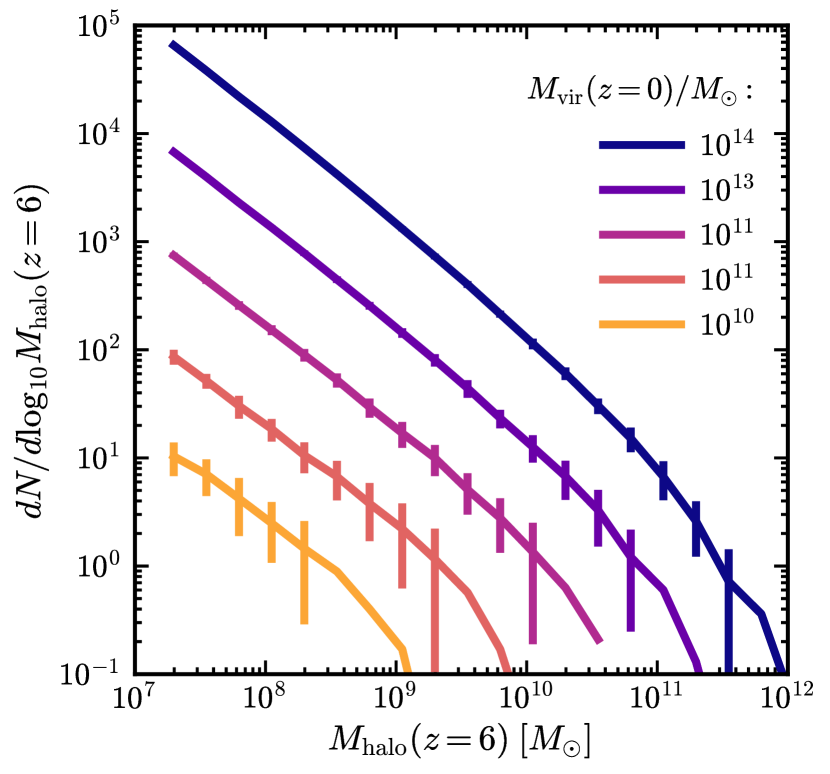
Figure 1: The average conditional (progenitor) dark matter halo mass function at $z=6$ for a variety of $z=0$ halo masses. Note the similarity in shapes and that the normalization at fixed $M_{\rm halo}(z=6)$ scales linearly with $M_{\rm{vir}}(z=0)$.

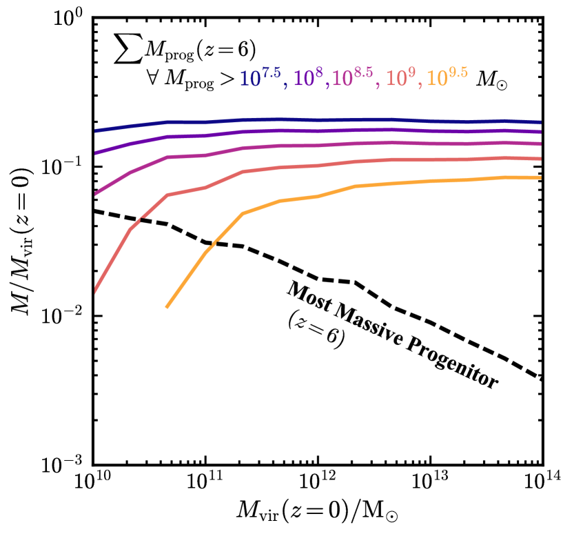
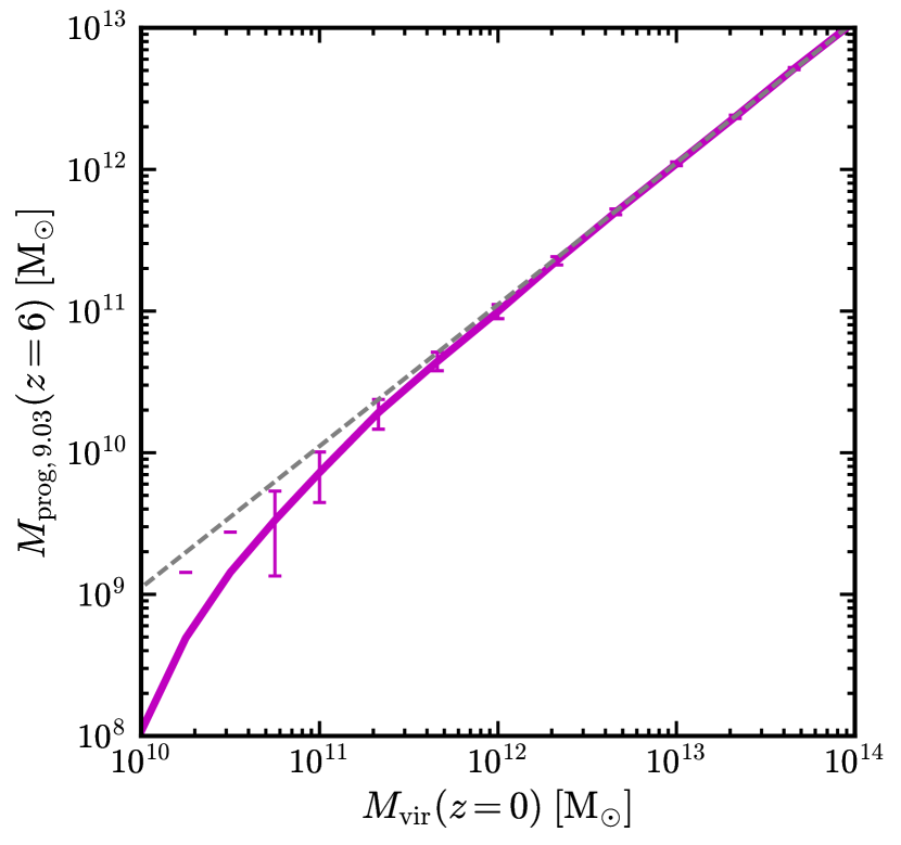
Figure 2: Left: A comparison of the halo mass contained within progenitors above given thresholds at $z=6$ ($M_{\rm prog,X}$; solid lines) with the average mass of a halo’s main progenitor at $z=6$ (dashed line), both relative to the $z=0$ halo mass. While the ratio of most massive progenitor to $z=0$ mass declines with $M_{\rm halo}(z=0)$, $M_{\rm prog,X}/M_{\rm halo}(z=0)$ is essentially constant over the entire range. Furthermore, the absolute value of $M_{\rm prog,X}/M_{\rm halo}(z=0)$ only differs by a factor of $\approx 2$ across 2 decades in threshold mass. Models directly relating $M_{\rm prog,X}$ to $M_{\rm GCs}$ naturally reproduce the observed correlation between $M_{\rm GCs}$ and $M_{\rm halo}(z=0)$. Right: The sum of $M_{\rm halo}$ over all progenitors with $M_{\rm halo}(z=6)>M_{\rm min}=1.07\times 10^{9}\,M_{\odot}$ as a function of $M_{\rm halo}(z=0)$. The dashed line shows $M_{\rm prog,9.03}\propto M_{\rm halo}(z=0)$. For $M_{\rm halo}\gg M_{\rm min}$, there is a one-to-one correlation. At lower masses, the halo-to-halo scatter becomes relevant, and below $M_{\rm{vir}}(z=0)\approx 3\times 10^{10}\,M_{\odot}$, many $z=0$ halos do not have even 1 progenitor above $M_{\rm min}$. See Eq. (24) for a fitting formula for $M_{\rm prog,9.03}$ given $M_{\rm halo}(z=0)$.

3.2 Evolving to $z=0$

At $z=0$, halos are composed of many progenitors of mass $M_{\rm prog}(z)<M_{\rm halo}(z=0)$. If (metal-poor) globular cluster formation is limited solely to the reionization era, then relations imprinted on the dark matter halo population at $z=6$ can be propagated to $z=0$ simply by understanding the dark matter assembly histories of $z=0$ halos. In particular, the total mass in globular clusters stars as a function of halo mass is simply the sum of the mass in GCs in progenitors above $M_{\rm min}$ (ignoring, for now, GC disruption):

$$M_{\rm GCs}(z=0)=\sum_{i}M_{\rm GCs}^{i}(z=6)\,,$$ (8)

where the sum is performed over all progenitors having $M_{\rm halo}^{i}(z=6)>M_{\rm min}$. The average mass in globular clusters in a halo as a function of $M_{\rm halo}(z=0)$ will be

$$\langle M_{\rm GCs}|M_{\rm halo}(z=0)\rangle =\sum_{i}\langle M_{\rm GCs}|M_{\rm halo}^{i}(z=6)\rangle$$ (9)

$$=\langle m_{\rm GC}(z=0)\rangle\sum_{i}\frac{M_{\rm halo}^{i}}{M_{\rm min}}\,f\left(\frac{M_{\rm halo}^{i}}{M_{\rm min}}\right)$$ (10)

$$\equiv\langle m_{\rm GC}(z=0)\rangle\frac{M_{\rm prog,X}(z=6)}{M_{\rm min}}\,.$$ (11)

In other words, the total mass of globular cluster stars in a halo of mass $M_{\rm halo}$ at $z=0$ is directly related to the sum of the masses of all its progenitor halos with $M(z=6)>M_{\rm min}$. In the nomenclature I adopt, $M_{\rm prog,X}$ is the sum in progenitors at $z=6$ with $\log_{10}(M/M_{\odot})>X$.

The minimum mass of a halo hosting a GC at high $z$ is defined by $M_{\rm min}=10^{X}$. Equating Eq. 3 and Eq. 11 yields

$$M_{\rm min}=\frac{\langle m_{\rm GC}\rangle}{\eta_{\rm b}}\,\frac{M_{\rm prog,X}}{M_{\rm halo}(z=0)}=10^{10}M_{\odot}\,\frac{M_{\rm prog,X}}{M_{\rm halo}(z=0)}\,,$$ (12)

where the second equality follows from my default assumptions of $m_{\rm GC}=2.5\times 10^{5}\,M_{\odot}$ and $\eta_{\rm b}=2.5\times 10^{-5}$. Note that Eq. 12 is sensitive to the combination $\langle m_{\rm GC}\rangle/\eta_{\rm b}$ and that there is implicit dependence on $M_{\rm min}$ in $M_{\rm prog,X}$.

The full results of the merger trees give $M_{\rm prog,X}(M_{\rm min})$: at $z=6$, the dependence of $M_{\rm prog,X}$ on $M_{\rm min}$ can be approximated by

$$\frac{M_{\rm prog,X}}{M_{\rm halo}(z=0)}=0.11\,(M_{\rm min}/10^{9}\,M_{\odot})^{-0.184}$$ (13)

to better than 5% accuracy over the range $10^{7.5}<M_{\rm min}/M_{\odot}<10^{9.5}$. I therefore obtain

$$M_{\rm min}(z=6)\approx 1.07\times 10^{9}\,M_{\odot}$$ (14)

(i.e., $X=9.03$). As is shown in Figure 2, such a model actually does give a linear correlation with $M_{\rm{vir}}(z=0)$, essentially irrespective of the mass threshold ($M_{\rm min}$) chosen. This is a natural outcome of cosmological models with CDM-like power spectra, as it is a feature of the high-redshift conditional mass function of $z=0$ halos (which can be calculated using extended Press-Schechter theory; e.g., Lacey & Cole 1993; van den Bosch 2002; see Fig. 1).

A model in which globular clusters populate all dark matter halos above $M_{\rm min}(z=6)\approx 10^{9}\,M_{\odot}$ in direct proportion to $M_{\rm halo}(z=6)$ naturally reproduces the observed $M_{\rm halo}-M_{\rm GCs}$ relation at $z=0$.

Eq. 12 can be split into dependence on dark matter properties [through $M_{\rm prog,X}/M_{\rm halo}(z=0)$] and baryonic properties (via $\langle m_{\rm GC}\rangle/\eta_{\rm b}$). Any redshift dependence enters solely through the relationship between the mass in collapsed progenitors above a given threshold at redshift $z$ ($M_{\rm prog,X}$). In this work, I assume that the epoch of blue globular cluster formation ends at $z=6$, and therefore this is the relevant redshift. It is straightforward to quantify the redshift dependence of Eq. 12, however: I find

$$\log_{10}(M_{\rm min}(z)/M_{\odot})=-0.165\,z+10.04\,.$$ (15)

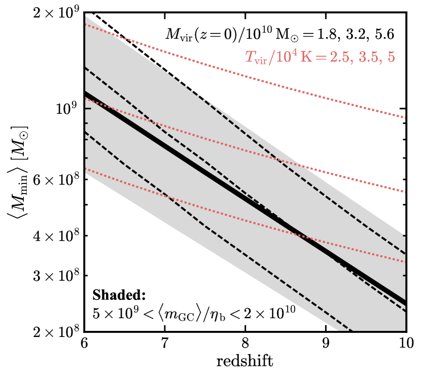
Figure 3: The dependence of $M_{\rm min}$ on redshift. Thick solid line: $M_{\rm min}(z)$, as obtained from solving Eq. 12. Shaded region: same, but allowing for a factor of 2 variation (both high and low) in $\langle m_{\rm GC}\rangle/\eta_{\rm b}$. Dashed black lines: the average mass assembly histories for halos with $M_{\rm{vir}}(z=0)/10^{10}\,M_{\odot}=1.8,\,3.2,\,5.6\,M_{\odot}$. Dotted orange lines: halos having virial temperatures of $T_{\rm vir}/10^{4}\,{\rm K}=2.4,\,3.5,\,5$. The evolution of $M_{\rm min}(z)$ is closely tracked by the evolution of the most massive progenitor of a typical halo with $M_{\rm{vir}}(z=0)\approx 2.5\times 10^{10}\,M_{\odot}$.

Figure 3 shows how $M_{\rm min}$ depends on the inferred epoch of globular cluster formation. The redshift evolution of $M_{\rm min}$ is can be well-approximated by the redshift evolution of the most massive progenitor ($M_{\rm mmp}$) of halos having $M_{\rm{vir}}(z=0)\approx 2.5\times 10^{10}\,M_{\odot}$. Independent of the redshift we chose to assign to GC formation, we will end up with the same relationship between $M_{\rm halo}(z=0)$ and the mass of the globular cluster system. The gray band in the figure shows the results of varying $\langle m_{\rm GC}\rangle/\eta_{\rm b}$ by a factor of $\pm 2$ from the fiducial value of $10^{10}\,M_{\odot}$.

The model laid out in this section is extremely simple: the total mass in globular clusters is directly proportional to halo mass at high redshift, with a minimum halo mass $M_{\rm min}$ capable of hosting 1 globular cluster of $M_{\rm min}\approx 10^{9}\,M_{\odot}$ at $z=6$. Halos for which $M_{\rm mmp}(z)\gg M_{\rm min}(z)$ will be insensitive to this cut-off. Halos with $M_{\rm mmp}(z)\approx M_{\rm min}(z)$ will be stochastically populated with globular clusters. Although this model is purely phenomenological rather than rooted in the detailed physics of globular cluster formation, its simplicity means that I can make several predictions about globular clusters and galaxy formation. These predictions and their implications are explored in subsequent sections.

4 Implications and Predictions at High Redshifts

4.1 Prospects for Observing High-$z$ Globular Clusters

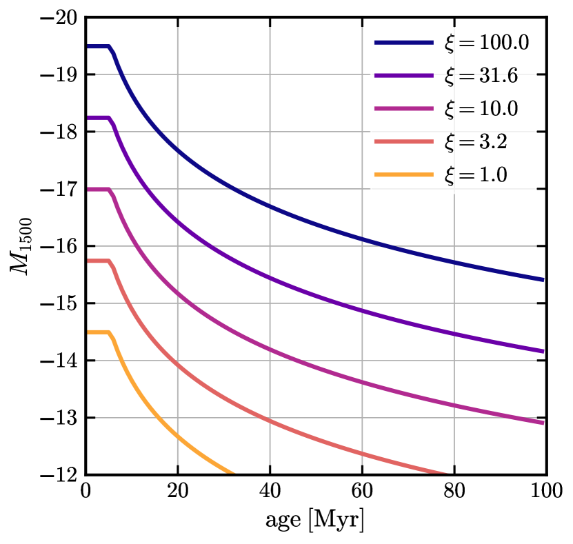
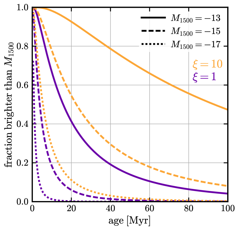
Figure 4: Left: the absolute UV magnitude of a globular cluster with birth mass $M_{\star}=\xi\times\,2.5\times 10^{5}\,M_{\odot}$ as a function of time after birth. $L_{1500}$ has a plateau for 5.5 Myr, then falls off as $t^{-1.3}$. Right: the fraction of globular clusters (with GC mass function given by Eq. (1)) brighter than various $M_{1500}$ thresholds as a function of time after completion of GC star formation for $\xi=1$ (purple) and $\xi=10$ (orange). This quantity is $f(<{M_{\rm 1500}}|\Delta t)$, which enters Eq. (22). The effective duty cycle of the GC mass function (i.e., what fraction of GCs can be observed at a given time) is given by $f(<{M_{\rm 1500}}|\Delta t)\,\Delta t/t_{\rm form}$, where $t_{\rm form}$ is the period over which all GCs form.

The ansatz of this paper – that the average mass in metal-poor GCs in a $z=0$ dark matter halo is directly related to the total dark matter mass in its progenitors above a fixed threshold in the reionization era – provides the means to compute the comoving number density of globular clusters: this is simply the comoving mass density of halos with $M_{\rm halo}(z=6)\geq M_{\rm min}$ divided by $M_{\rm min}$:

$$n_{\rm GCs}=\frac{1}{M_{\rm min}}\int_{M_{\rm min}}^{\infty}dM\,M_{\rm halo}\,\frac{dn_{\rm halo}}{dM_{\rm halo}}\,.$$ (16)

At $z=6$, $M_{\rm min}=1.07\times 10^{9}\,M_{\odot}$, implying a comoving cumulative number density of $n_{\rm GCs}=2.2\,{\rm Mpc}^{-3}$ for blue globular clusters (using the Sheth et al. 2001 mass function).

With this number, we can investigate the observability of high-redshift galaxy formation as traced by globular clusters. Assuming a Kroupa (2001) stellar initial mass function, $[{\rm Fe/H}]=-2$, either Padova (Marigo et al., 2008; Girardi et al., 2010) or MIST (Dotter, 2016; Choi et al., 2016) stellar evolution models (see below) and a 5 Myr duration for star formation (with constant $\dot{M}_{\star}$), a globular cluster will have an absolute rest-frame magnitude at 1500 Å($M_{1500}$) that can be approximated by

$$M_{1500}(t) =-16.75-2.5\,\log_{10}\left(\frac{M_{\star}}{2\times 10^{6}\,M_{\odot}}\,g(t)\right)$$ (17)

$$g(t) =\begin{cases}1\;&{\rm if}\;t<5.5\,{\rm Myr}\\ \left(\frac{t}{5.5\,{\rm Myr}}\right)^{-1.3}&{\rm if}\;5.5\leq t/{\rm Myr}\la 300\\ \end{cases}$$ (18)

This result is based on calculations using the Flexible Stellar Population Synthesis models of Conroy et al. 2009; Conroy & Gunn 2010, including nebular emission (Byler et al., 2017), and is fairly insensitive to the choice of stellar models: the rms deviations from the fit are 0.10 mag and 0.16 mag and the maximal deviation from the fit is 0.32 mag and 0.37 mag for Padova and MIST models, respectively, for $t<300\,{\rm Myr}$. I caution against using Eq. 17 for ages beyond 300 Myr, as the errors become substantial. In the future, it will be important to consider variations in stellar models that include, e.g., binaries or fast-rotating massive stars, as these models predict a different peak value and evolution of ${M_{\rm 1500}}$ with time.

The number of GCs in the redshift range $(z_{1},z_{2})$ is

$$N(z_{1},z_{2})=\int_{z_{1}}^{z_{2}}n(z)\,dV\,.$$ (19)

If GCs form with a uniform distribution in time over the interval $(z_{1},z_{2})$, then Eq. 19 becomes

$$N(z_{1},z_{2}) =\frac{n_{\rm GCs}}{t(z_{1},z_{2})}\int_{z_{1}}^{z_{2}}t(z_{1},z)\frac{dV}{dz}{dz}\,$$ (20)

$$\equiv n_{\rm GCs}V(z_{1},z_{2})\,\zeta(z_{1},z_{2})\,,$$ (21)

where $V(z_{1},z_{2})$ and $t(z_{1},z_{2})$ are the comoving volume and cosmic time, respectively, between redshifts $z_{1}$ and $z_{2}$; $\zeta(z_{1},z_{2})$ encapsulates the effect of a changing number of GCs with $z$, i.e., how much $N(z_{1},z_{2})$ differs from the naive estimate of $n_{\rm GC}\,V(z_{1},z_{2})$ owing to the time evolution of $n_{\rm GC}(z)$. Unless otherwise noted, I assume that GCs form with a uniform distribution in time over $10\geq z\geq 6$ ($t(z_{1},z_{2})=457$ Myr). The correction factor $\zeta$ is non-negligible, as it has a maximum value of $0.5$ (obtained in the limit $z_{1}\approx z_{2}$). I find $\zeta(z_{1}=10,\,z_{2}=6)=0.44$.

The number of observable GCs in a field of angular size $\Omega$ is then approximately

$$N(<{M_{\rm 1500}})=N(z_{1},z_{2})\left(\frac{\Omega}{\rm 4\pi\,sr}\right)\,\frac{\Delta t}{t(z_{1},z_{2})}\,f({<{M_{\rm 1500}}|\Delta t})\,,$$ (22)

where $\Delta t$ is the time period for which a GC exceeds the given ${M_{\rm 1500}}$ threshold and $f(<{M_{\rm 1500}}|\Delta t)$ is the fraction of globular clusters brighter than ${M_{\rm 1500}}$ for a period of at least $\Delta t$ using Eqns. (1) and 17. $N(<{M_{\rm 1500}})$ is therefore a trade-off between the observability period $\Delta t$ (which is longer for more massive GCs) and the fraction of globular clusters brighter than ${M_{\rm 1500}}$ for a time period of at least $\Delta t$ (which is a decreasing function of $\Delta t$). Note that for a lognormal distribution of GC masses, as assumed here, $\sim 4.8\%$ of GCs will have masses larger than 10 times the median (turnover) mass. For $\xi=1$, this means 5% of GCs will reach ${M_{\rm 1500}}<-17$. If $\xi=10$, then 5% will reach ${M_{\rm 1500}}=-19.5$ (for approximately 5 Myr) and 50% of GCs will reach ${M_{\rm 1500}}=-17$!

Table 1: Observability of globular clusters at high redshifts. The entries in the table give the number of globular clusters brighter than the absolute magnitude listed in column 1 for various values of $\xi$ (the average value of the ratio of birth mass to $z=0$ mass). The numbers quoted here assume $\Omega=5\,{\rm arcmin^{2}}$, comparable to the size of ACS on HST. For JWST, the numbers below should be multiplied by 2 ($\Omega=9.7\,{\rm arcmin}^{2}$). At $z=6$, $M_{1500}=-15$ corresponds to $m_{1500}=31.7$; this is approximately the reach of a JWST ultra-deep survey (200 hr).

	Number of Detectable Globular Clusters in $5\,{\rm arcmin^{2}}$
	$(6\leq z\leq 10)$
$M_{1500}$	$\xi=1$	3.16	10	31.6	100
-17	20	48	116	282	684
-16	40	97	236	573	1389
-15	82	198	480	1163	2435
-14	166	402	974	2173	3314
-13	337	816	1906	3129	3796

The expected number of GCs detectable for various $M_{1500}$ thresholds are listed in Table 1 for $\Omega=5\,{\rm arcmin}^{2}$, roughly comparable to the field of view of ACS on the Hubble Space Telescope (HST). The numbers in Table 1 are not very sensitive to the assumed redshift range of globular cluster formation (so long as the lower limit is $z\approx 5-6$): for example, the quoted numbers should be multiplied by a factor of 1.09 if $6\leq z\leq 7$ or 0.87 if $5\leq z\leq 15$. $N_{\rm GCs}$ scales linearly with $\Omega$, so for a field the size of NIRCam on the James Webb Space Telescope (JWST) – $9.7\,{\rm arcmin}^{2}$ – the numbers are approximately double those listed in the table.

In fact, many of the faintest gravitationally-lensed sources observed at $z\sim 6-8$ are consistent with small sizes (Bouwens et al., 2017; Vanzella et al., 2017), perhaps indicating that globular clusters are the easiest objects to detect at high redshift. At a minimum, a JWST survey reaching $M_{1500}=-15$ ($m=31.7$) should observe $\approx 160$ forming GCs per field. If $\xi>1$, the number will be larger: for example, if $\xi=10$, then $N_{\rm GCs}\approx 1000$ per field. Of these, essentially all are expected to be in separate dark matter halos – on average, $\la 1$ halo in this volume will be massive enough to host $>1$ detectable GC at a time. The number of GCs will therefore provide a probe of the halo mass function at high redshifts. It is important to note that, in this context, GCs are not really distinct from galaxies; rather, it is the large quantity of stars formed in a short time in a globular cluster that makes a globular the easiest part of a galaxy to see. An important distinction between GCs and “normal” star formation is that the standard conversion from UV flux to star formation rate (Kennicutt, 1998; Madau & Dickinson, 2014) assumes extended star formation of $t_{\rm sf}>10^{7}\,{\rm yr}$, which is not true for GCs. In the model under discussion, GCs are forming in dark matter halos, but likely not at their centers (thereby accounting for their observed lack of dark matter).

HST surveys of the UDF have revealed approximately 150 galaxies at $z\ga 6$ with $M_{1500}\la-17$ (Bouwens et al., 2015; Finkelstein et al., 2015). The numbers in Table 1 immediately disfavor models with $\xi\ga 15$: if globular cluster birth masses were $\ga 15$ times their present-day masses, the HUDF would have many more high-$z$ detections compared to what is actually observed. Even $\xi\approx 10$ implies that $\ga 70\%$ of detections at $z\ga 6$ are globular clusters rather than “normal” star formation in high-$z$ galaxies. The results presented here therefore strongly suggest that the birth masses of globular clusters exceed their present-day stellar masses by less than a factor of ten. The number counts and size distribution of ${M_{\rm 1500}}\ga-16$ objects at $z\approx 6-10$ in JWST blank fields will provide a stringent test of whether or not metal-poor GCs are much less massive than they were at birth.

Based on the arguments above, the stellar mass completeness of UV-selected galaxy samples at high redshift will be strongly influenced by globular clusters for ${M_{\rm 1500}}\ga-16$. One globular cluster that forms $\sim 10^{6}\,M_{\odot}$ of stars in a nearly instantaneous burst ($t\approx 5\,{\rm Myr}$) with $\dot{M}_{\star}\approx 0.2\,M_{\odot}\,{\rm yr^{-1}}$ and then fades passively will move from ${M_{\rm 1500}}\approx-16.5$ immediately following the burst to ${M_{\rm 1500}}\approx-14$ within 40 Myr. Note that a galaxy that forms $10^{6}\,M_{\odot}$ of stars at a constant rate over a (current) Hubble time will have a star formation rate of $10^{-4}\,M_{\odot}\,{\rm yr^{-1}}$, which would correspond to ${M_{\rm 1500}}\approx-7.5$. Even if all of the $10^{6}$ stars formed over a (relatively) short period of 1 Gyr ($\dot{M}_{\star}\approx 10^{-3}\,M_{\odot}\,{\rm yr^{-1}}$), which is even shorter than duration inferred for the Draco dwarf spheroidal galaxy, it would only result in ${M_{\rm 1500}}\approx-10$ while the galaxy is actively forming stars. These considerations are relevant when considering the importance of galaxies versus GCs as very faint sources (below HST detection thresholds) when constructing UV luminosity functions and interpreting them in the context of reionization.

4.2 Connections with Cosmic Reionization

Using the average mass of a GC, we can also compute the stellar mass density in GCs; this is $\rho_{\rm GCs}=\langle m_{\rm GC}\rangle\,n_{\rm GCs}=\xi\times 5.5\times 10^{5}\,M_{\odot}\,{\rm Mpc}^{-3}$ at $z=6$. This number can be related to the importance of GCs for reionization (e.g., Ricotti 2002; Schaerer & Charbonnel 2011; Katz & Ricotti 2013). The star formation rate density required to maintain an ionized IGM is given by

$$\dot{\rho}_{\star}=1.2\times 10^{-3}\left(\frac{C}{f_{\rm esc}}\right)\left(\frac{1+z}{8}\right)^{3}\,M_{\odot}\,{\rm yr^{-1}}\,{\rm Mpc}^{-3}\,.$$ (23)

(see eq. 27 of Madau et al. 1999; $C$ is the clumping factor of the intergalactic medium and $f_{\rm esc}$ is the escape fraction of ionizing photons). If we assume that metal-poor GCs form over the epoch $z=10$ to $z=6$, integrating equation 23 gives a requisite stellar mass to maintain reionization over that period of $\sim 7.2\times 10^{5}\,M_{\odot}\,{\rm Mpc}^{-3}\,(C/f_{\rm esc})$. GCs therefore provide a fraction $0.76\,\xi\,f_{\rm esc}\,C^{-1}$ of the ionizing flux needed to maintain reionization.

Fiducial models often assume $C=3$ and $f_{\rm esc}\approx 0.2$ (e.g., Robertson et al. 2015; McQuinn 2016), with uncertainties in $f_{\rm esc}$ dominating those in $C$ (e.g., Ma et al. 2015). GCs may have even higher escape fractions of $f_{\rm esc}\ga 0.5$ (Ricotti, 2002), in which case, GCs are likely major contributors to reionization irrespective of $\xi$. Similarly, if $\xi\approx 10$, GCs are important reionization sources so long as $f_{\rm esc}\ga 0.1$ (and potentially dominant if $f_{\rm esc}\ga 0.2$ for GCs). Even if $\xi\approx 5$, GCs may provide the bulk of ionizing photons at early times if $f_{\rm esc}\ga 0.3$. If both $\xi$ and $f_{\rm esc}$ are small, GCs do not significantly contribute to reionization , though they still may play an important role in their immediate environments. Understanding the relationship between the stellar mass at birth and at present is therefore a pressing question for cosmology as well as for star formation.

In passing, I note that $M_{\rm{vir}}(z=6)\approx 10^{9}$ – the minimum mass of a halo hosting one dark matter halo as derived above – corresponds to ${M_{\rm 1500}}\approx-13$ in abundance-matching models (Kuhlen & Faucher-Giguère, 2012; Boylan-Kolchin et al., 2014; Boylan-Kolchin et al., 2015; Boylan-Kolchin et al., 2016); this is approximately the UV luminosity at which Boylan-Kolchin et al. (2014); Boylan-Kolchin et al. (2015) and Weisz & Boylan-Kolchin (2017) argue there should be a break in the high-$z$ galaxy luminosity function based on the stellar fossil record in the Local Group. The connection between the mass required to host, on average, 1 GC and the turn-over halo mass for the high-$z$ UVLF is no more than circumstantial at this point, but it is not difficult to imagine a scenario in which halos above some critical mass have multiple channels for star formation (e.g., “normal” star formation and GC star formation) while those below the mass scale do not achieve the high gas densities required for GC formation. This issue will be addressed in a future paper.

4.3 Constraining the Dark Matter Power Spectrum

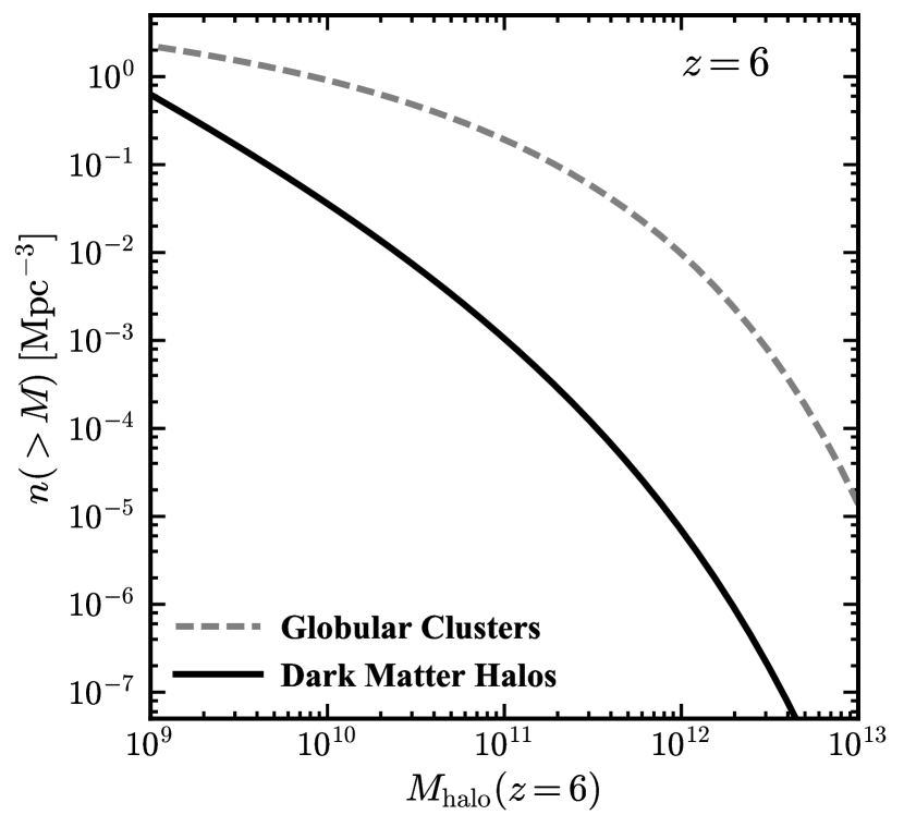
Figure 5: The cumulative number density of dark matter halos (solid black line) and globular clusters (dashed gray line) as a function of halo mass at $z=6$ according to the model presented in this paper. A single source detected with implied cumulative number density of $1\,{\rm Mpc}^{-3}$ could either be a galaxy in a $7\times 10^{8}\,M_{\odot}$ halo or a GC in a $10^{10}\,M_{\odot}$ halo. The possibility of detecting globular clusters at high $z$ therefore complicates the ability to use UV luminosity functions to constrain dark matter models, as the basic assumptions of abundance matching break down.

Various authors have pointed out that high-redshift galaxy luminosity functions can serve as strong constraints on any cut-off in the dark matter power spectrum at wavenumbers corresponding to halo masses of $M_{\rm{vir}}\approx 10^{8-9}\,M_{\odot}$ (Schultz et al., 2014; Bozek et al., 2015; Menci et al., 2017). The basic idea is straightforward: by assuming galaxies populate halos with a monotonic mapping between ${M_{\rm 1500}}$ and $M_{\rm halo}$, the existence of faint galaxies necessarily implies a population of low-mass halos. Current results using this technique appear to rule out much of the parameter space in which Warm Dark Matter models produce appreciably different structure than Cold Dark Matter models (Schultz et al., 2014; Menci et al., 2017); similarly, models of “fuzzy dark matter” (Hu et al., 2000; Hui et al., 2017) that naturally produce kpc-scale cores in dwarf galaxies at low-$z$ may not have enough structure at high-$z$ to produce the abundance of observed galaxies (Bozek et al., 2015).

If, however, GCs are significant contributors to the UV luminosity function – as the results in this paper suggest – then the true constraints are likely significantly weaker. The detection of a single galaxy with an implied cumulative number density of $1\,{\rm Mpc}^{-3}$, which would rule out models that suppress power on scales $\la 10^{9}\,M_{\odot}$ in standard abundance matching models, can easily be attributed to a GC in a much more massive halo that is caught $\sim 20\,{\rm Myr}$ after its peak star formation. As is shown in Figure 5, $N_{\rm GCs}(>M_{\rm halo})\approx 1\,{\rm Mpc}^{-3}$ is attained at a halo mass that is an order of magnitude greater than the halo mass corresponding to $n(>M_{\rm halo})\approx 1\,{\rm Mpc}^{-3}$ ($M_{\rm halo}\sim 10^{10}\,M_{\odot}$ versus $M_{\rm halo}\approx 10^{9}\,M_{\odot}$).

4.4 Efficiency of Globular Cluster Star Formation

The linear relationship between the present-day mass in GCs and the sum of $z\sim 6$ dark matter halo mass in halo progenitors indicates that GCs form at a constant efficiency in the high-redshift universe. With a universal baryon fraction of $f_{\rm b}=\Omega_{\rm b}/\Omega_{\rm m}\approx 0.156$, and assuming that globular clusters had stellar masses at formation of $\xi\,m_{\rm GC}(z=0)$, I obtain a baryon conversion efficiency of $\xi\,\langle M_{\rm GC}\rangle/(f_{\rm b}\,M_{\rm min})$. If $\xi$ is large ($\xi\approx 10-20$), then the baryon conversion efficiency into old globular cluster stars is also large ($\approx 1.4-2.8\%$), meaning $\sim 2\%$ of baryons in dark matter halos more massive than $M_{\rm min}$ at $z\approx 6$ are converted into stars in blue globular clusters. If $\xi\approx 1-2$, then closer to $0.1\%$ of baryons in these dark matter halos are converted into stars in blue GCs.

5 Implications and Predictions at Low Redshift

5.1 Globular clusters in low-mass dark matter halos

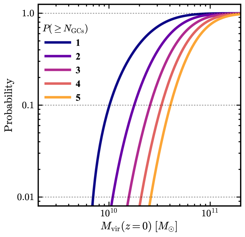
Figure 6: Probability distributions for hosting at least $N$ globular clusters as a function of halo mass at $z=0$ according to the model presented in Section 5.1. The mass at which $P(\geq 1\,{\rm GC})=0.5$ is $2.1\times 10^{10}\,M_{\odot}$. At lower masses, the probability of hosting a globular cluster is strongly suppressed in this model.

A simple model for globular clusters in dark matter halos at $z=0$ is that the mean mass in globular cluster stars as a function of halo mass is $\langle m_{\rm GC}\rangle\,M_{\rm prog,9.03}/M_{\rm min}$ (with $M_{\rm min}=10^{9.03}\,M_{\odot}$; see Eq. 14). The right panel of Figure 2 shows the dependence of $M_{\rm prog,9.03}$ on $M_{\rm halo}(z=0)$; a good fit is given by

$$M_{\rm prog,9.03}=0.11\,M_{\rm halo}\,\left[1-\left(\frac{M_{\rm halo}}{A\times 10^{9.03}\,M_{\odot}}\right)^{-b}\right]^{1/b}\,,$$ (24)

with $A=6$ and $b=0.575$.

Observationally, the scatter in the mass in globular clusters at fixed halo mass is approximately constant with $\sigma\la 0.28$ dex. A plausible model for such a relation is the negative binomial distribution, which can be parametrized by a mean value and a (constant) intrinsic scatter (see Boylan-Kolchin et al. 2010). In the limit that the intrinsic scatter goes to zero, the negative binomial distribution converges to a Poisson distribution. I therefore assume that the mass in GCs is given by $\langle m_{\rm GC}\rangle\,N_{\rm GCs}$ and that $N_{\rm GCs}$ is described by a negative binomial distribution with a mean value of

$$\langle N\rangle=\frac{M_{\rm prog,9.03}}{1.07\times 10^{9}\,M_{\odot}}\,$$ (25)

and an intrinsic scatter of 40%. This toy model reproduces the observed $M_{\rm GCs}-M_{\rm halo}$ relationship and its observed $0.28\,{\rm dex}$ scatter (Harris et al. 2017, assuming a scatter of $0.2\,{\rm dex}$ in the stellar mass-halo mass relationship; Hudson et al. 2014).

Figure 6 shows how the probability for hosting at least $N$ globular clusters varies as a function of halo mass at $z=0$ according to this model. At $M_{\rm{vir}}(z=0)=2.1\times 10^{10}\,M_{\odot}$, there is a 50% chance of hosting at least one blue GC. This probability drops precipitously at lower masses: 1 in 10 halos with $M_{\rm{vir}}(z=0)=1.01\times 10^{10}\,M_{\odot}$ will host at least one blue GC, while fewer than 1 in 100 halos with $M_{\rm{vir}}=7\times 10^{9}\,M_{\odot}$ will host a blue GC. These numbers are useful in the context of considering possible dwarf galaxy hosts of GCs near the Milky Way (Zaritsky et al., 2016) and the halo masses of dwarf galaxies known to host blue GCs, e.g., Eridanus II (Koposov et al., 2015; Crnojević et al., 2016) and Pegasus (Cole et al., 2017). More sophisticated (and perhaps more physically plausible) models of the occupation number of GCs as a function of $z=0$ halo mass might include the effects of environment on $P(N_{\rm GCs}|M_{\rm halo})$; for example, patchy reionization might contribute to scatter in formation redshifts for globular clusters (Spitler et al., 2012).

5.2 In-Situ versus accreted globular clusters

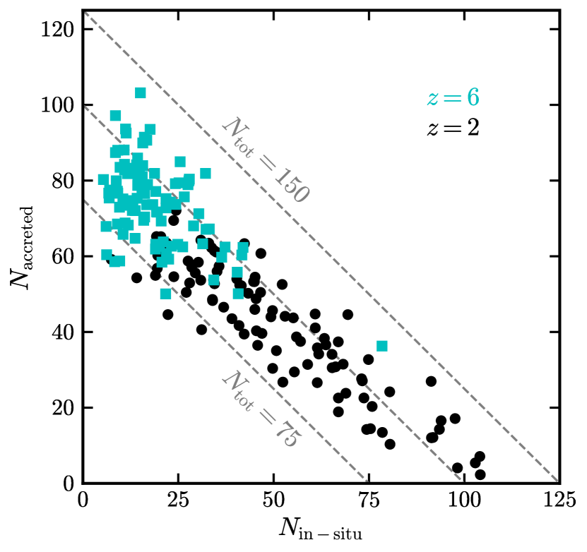
Figure 7: The number of in-situ globular clusters (those in the main progenitor) versus accreted GCs at $z=6$ (cyan) and $z=2$ (black) for Milky-Way-mass halos at $z=0$. At $z=6$, the majority of GCs are not in the main progenitor; by $z=2$, more than half of the realizations contain at least $50\%$ of the $z=0$ blue GCs in the main progenitor.

My model for globular cluster formation also enables a straightforward calculation of the fraction of globular clusters formed in-situ by a given redshift (i.e., that formed by redshift $z$ in the main progenitor of a $z=0$ halo) versus those that were formed in a separate halo and later accreted. The average fraction of in-situ clusters for a given halo mass at $z=6$ is simply $\langle M_{\rm mmp}\rangle/M_{\rm prog,9.03}$. The average fraction of in-situ clusters determined using any later redshift $z$ requires calculating the fraction of mass in progenitors at $z=6$ above $M_{\rm min}$ that ends up in the main progenitor at $z$; this is straightforward, given a merger tree.

Figure 7 shows the predicted number of in-situ versus accreted blue globular clusters for 100 realizations of Milky-Way-mass halos ($M_{\rm halo}(z=0)=10^{12}\,M_{\odot}$). The cyan points show results at $z=6$, while the black points show results for $z=2$. At early times, most of the globular clusters are not associated with the Milky Way’s main progenitor; in other words, most of the blue globular clusters of the present-day Milky Way were not formed in-situ. I find that, on average, 16.6% of GCs found in the Milky Way today were formed in its main progenitor by $z=6$, with a 90% confidence interval of 8-40%. The upper end of this range agrees with the somewhat different models of Katz & Ricotti (2014). The typical accreted GC came in as part of a relatively low-mass progenitor: the average dark matter halo contributing to the accreted population hosts 2 GCs, and there are typically $\sim 30$ such progenitors. If we consider $z=2$, there is a much broader range of possibilities, from the vast majority of the Milky Way’s blue GCs already residing in the main progenitor to the majority coming from accretion subsequent to $z=2$. In general, halos with earlier assembly histories will have a larger fraction of their globular clusters in place (in situ) at a given redshift. Since the Milky Way appears to have a relatively quiescent recent merger history, it may tend toward the region of Figure 7 that is dominated by in-situ globulars at $z=2$.

Another interesting regime is the low-$M_{\rm halo}$ end of the $M_{\rm halo}-M_{\rm GCs}$ relation (see also Zaritsky et al. 2016). This is particularly true in the context the Fornax dwarf spheroidal galaxy, which has 5 globular clusters (4 of which are metal-poor), all of which reside within 2 kpc of the galaxy’s center (in projection; Mackey & Gilmore 2003; de Boer & Fraser 2016). The very existence of these globulars is somewhat surprising on multiple levels: the implied specific frequency of GCs in Fornax is very high (e.g., Georgiev et al. 2009), and furthermore, dynamical friction should have caused them to spiral to the center of the galaxy if they have been present in the galaxy for a Hubble time (Tremaine, 1976; Oh et al., 2000). One explanation of their survival is that Fornax has a cored dark matter distribution (Goerdt et al., 2006); alternatively, perhaps the globular clusters in Fornax have been accreted on a cosmologically recent timescale (e.g., Cole et al. 2012), in which case the dynamical friction arguments would be weakened substantially.

In the context of the model presented here, it is extremely unlikely that all four of Fornax’s metal-poor were accreted recently. At $M_{\rm halo}\approx 3\times 10^{10}\,M_{\odot}$, 2% of merger tree realizations have at least 4 GCs. Of these 2%, approximately 1/4 have at least 2 accreted (post $z=6$) GCs, but all of these have at least 2 in-situ clusters as well. Only 0.2% of the realizations have even one GC accreted after $z=2$. This is a consequence of the relatively sharp cut-off in the abundance of globulars in galaxies below the mass of Fornax.

Harris et al. (2017) noted that the $M_{\rm GCs}-M_{\rm halo}$ relation predicts a halo mass of $\sim 1.5\times 10^{10}\,M_{\odot}$ for Fornax, while many dynamical estimates of its halo mass based on stellar kinematics indicate a much lower mass ($0.5-1\times 10^{9}\,M_{\odot}$; Peñarrubia et al. 2008; Kuhlen 2010; Boylan-Kolchin et al. 2012). They interpreted this as a possible break down in the $M_{\rm GCs}-M_{\rm halo}$ relation for low-luminosity galaxies. However, the $M_{\rm GCs}-M_{\rm halo}$ prediction for Fornax’s halo mass is roughly in line with abundance matching expectations (Garrison-Kimmel et al., 2017; Read et al., 2017), perhaps indicating that the constancy of $\eta_{\rm b}$ persists even to the dwarf galaxy regime. It is important to note that dynamical estimates of Fornax’s mass are based on stellar kinematics, which only extend to $\sim 1$ kpc from its center. In $\Lambda$CDM, Fornax should be embedded in a much more extended (and massive) dark matter halo, reconciling its apparently low halo mass with the $M_{\rm GCs}-M_{\rm halo}$ relationship. The high specific frequency of globular clusters in Fornax and other dwarf galaxies is somewhat of a red herring in this model: it is an outcome of the low overall star formation efficiency (per halo mass) in dwarf galaxies combined with the constant globular cluster star formation efficiency.

6 Summary

The possible association of (metal-poor) globular clusters with dark matter halos has a venerable history, starting with Peebles (1984). Rosenblatt et al. (1988) suggested that associating GCs with $2.8\,\sigma$ density fluctuations in CDM models naturally reproduces, to first order, various properties of the Milky Way’s GC system. Moore et al. (2006) argued that the spatial distribution and kinematics of both GCs and dwarf galaxies in the Milky Way is indicative of formation in peaks of at least $2.5\,\sigma$ in the density distribution (see also Boley et al. 2009; Corbett Moran et al. 2014). They also noted that “the mass fraction in peaks of a given $\sigma$ is independent of the final halo mass” above some minimum host mass.

In this paper, I present a phenomenological model that is rooted in this lineage. The model is simple: I assume that blue globular clusters form in halos above some minimum mass $M_{\rm min}$ by $z=6$ and that the mass in globular cluster stars formed is directly proportional to the dark matter halo mass at formation. GCs need not form at the centers of the halos (and likely do not, given existing constraints on the dark matter content of GCs); rather, they may be the subcomponents of a halo’s baryonic content that have fragmented out of compressed gas and would coexist with “normal” star formation in halos at high redshifts. In such a model, the linear correlation between $M_{\rm GCs}$ and $M_{\rm halo}$ at $z=0$ is naturally reproduced, which is a consequence of the mass assembly of CDM halos and the CDM power spectrum. This model also predicts the minimum mass of a dark matter halo capable of hosting one GC during the epoch of GC formation; for the parameters adopted here, it is $M_{\rm min}(z=6)=1.07\times 10^{9}\,M_{\odot}$ (with mild redshift dependence). Using this basic model, I explore a number of implications and predictions at both high and low redshifts:

• High-$z$ observability: I estimate the number density of old GCs to be $\approx 2\,{\rm Mpc}^{-3}$ using the formalism of Sections 2-3. If the epoch of formation for metal-poor GCs spans $10>z>6$, then high-$z$ globular cluster formation should be visible directly, as GCs are UV-bright for a period that depends only on the total mass in stars formed (i.e., on $\xi$, the ratio of GC birth mass to present-day mass). Indeed, 5% of GCs should be bright enough at formation to detect in the HUDF (${M_{\rm 1500}}=-17$) even if $\xi=1$. If $\xi=10$, 50% of GCs reach ${M_{\rm 1500}}=-17$ and 5% reach ${M_{\rm 1500}}=-19.5$ (albeit for only $\sim 5$ Myr).

  Eq. (22) gives the number of GCs observable in a field with fixed angular size; I estimate that 20 (116) GCs are already visible, with ${M_{\rm 1500}}<-17$, in the Hubble Ultra Deep Field if $\xi=1$ (10). JWST will likely be sensitive to $\sim 150-1000$ GCs in a survey that reaches ${M_{\rm 1500}}=-15$ ($m=31.7$ at $z=6$), depending on $\xi$. Given that only $\sim 150$ sources with ${M_{\rm 1500}}(z\ga 6)<-17$ have been detected in the UDF, I find that values of $\xi\ga 10$ are strongly disfavored. The HUDF therefore already provides an important constraint on the formation of GCs and the origin of their abundance patterns; JWST will almost certainly provide definitive data regarding $\xi$.

• Reionization: even with $\xi\approx 5$, metal-poor globular clusters may drive cosmic reionization so long as they have relatively high escape fraction ($f_{\rm esc}\ga 0.3$), as has previously been argued by Ricotti (2002); Schaerer & Charbonnel (2011); Katz & Ricotti (2013).

• Constraints on dark matter models: Many of the faintest sources at high redshifts in HST lensing fields appear to be extremely compact (Vanzella et al., 2017; Bouwens et al., 2017). If some non-negligible fraction of these sources are GCs in formation, then the constraints on dark matter models obtained by comparing the observed number density of galaxies to the predicted number density of dark matter halos are weakened substantially: observed sources may be bright proto-GCs in more massive halos rather than “typical” galaxies in less massive halos.

• Halo masses at low redshifts: The faintest galaxies hosting at least one globular cluster (e.g., Pegasus and Eridanus II) are very likely to be in halos with masses of $7\times 10^{9}\la M_{\rm halo}\la 3\times 10^{10}\,M_{\odot}$ at the present day.

• Accreted versus in-situ clusters: the fraction of metal-poor GCs formed in situ by $z=6$ varies strongly with halo mass, with all GC formation occurring in situ for the lowest-mass halos and most GCs being accreted for very massive (galaxy cluster) halos. Milky Way-mass systems form 17% of their old GCs in situ (in the main progenitor by the end of GC formation), with a 90% confidence interval of 8-40%. The typical accreted GC comes from a relatively low-mass progenitor hosting $\sim 2$ GCs. It is highly unlikely that all of the metal-poor GCs in the Fornax dSph were accreted in the past 10 Gyr.

Perhaps the most intriguing result of this paper is that HST observations are already constraining $\xi$ and that JWST will likely provide a definitive test of scenarios that require large populations of “first-generation” GC stars ($\xi\ga 10$). Even relatively low values of $3\la\xi\la 5$ imply that GCs may be dominant contributors to reionization. The need for obtaining more accurate ages of old globular clusters – a time-honored astronomical endeavor – is therefore pressing. As an example, accurate absolute age determinations with a precision of $\la 0.8$ Gyr would be able to differentiate consider two models, one in which globular clusters form at $6\ga z\ga 3$ ($0.93\la t_{\rm cosmic}\la 2.14$ Gyr) and another with a formation epoch of $10\la z\la 6$ ($0.47\la t_{\rm cosmic}\la 0.93$ Gyr).

I have not considered the effects of globular cluster disruption (e.g., Spitzer 1987; Vesperini & Heggie 1997; Gnedin et al. 1999; Trenti et al. 2010) in this work. The motivation for this – beyond convenience – is that it provides a conservative estimate on the observability of GCs in the reionization era and their effects on dark matter constraints. A future paper will include the effects of GC disruption and resulting implications for a variety of quantities, including the contribution of disrupted GCs to the stellar halos of galaxies (e.g., Boley et al. 2009). However, immediate constraints on disruption come from the scatter in the $M_{\rm GCs}-M_{\rm halo}$ relation. In particular, the mass dependence of the Harris et al. (2017) calibration of $\eta_{\rm b}$ is negligible, implying that either disruption is a minimal effect or is independent of halo mass (which would be unexpected, given the strong dependence of galaxy mass on halo mass). If disruption is indeed uniform across halo mass, the primary effect would be to modify the derived efficiency of conversion of baryons into globular clusters without affecting $M_{\rm min}$; the results presented in Section 4.4 are a lower limit. Such disruption would also affect the $M_{\rm halo}-M_{\rm GCs}$ relation at $z=6$, but not the relation at $z=0$ and could be fully incorporated into the present model through a parameter $f_{\rm disrupt}$ via $\xi\rightarrow f_{\rm disrupt}\,\xi$. Dissolution owing to two-body relaxation is likely to be an important effect for $m_{\rm GC}\ll 2\times 10^{5}\,M_{\odot}$ (i.e., below the characteristic mass of the $z=0$ globular cluster luminosity function; Fall & Zhang 2001). However, $M_{\rm GCs}$ is dominated by clusters above the characteristic mass, implying that evaporation of low-mass globular clusters is at most a second-order effect in establishing the observed $M_{\rm GCs}-M_{\rm halo}$ relation.

The model presented here is explicitly aimed at understanding metal-poor (blue) globular clusters. This is motivated by the overall dominance of metal-poor globular clusters over metal-rich ones and their earlier formation epoch (Forbes et al., 2015), which links them to the reionization era. Nevertheless, a full model for globular cluster formation should also explain metal-rich clusters and why they also scale linearly with halo mass (Harris et al., 2015). Merger-based formation models (e.g., Ashman & Zepf 1992; Bekki et al. 2008) are compelling in this context and will be the subject of forthcoming work.

A somewhat more speculative, but intriguing, future direction is to consider the predictions of the current model in the context of supermassive black hole formation. There is a well-established observational connection between the mass of a central black hole and $M_{\rm GCs}$ for galaxies (Spitler & Forbes, 2009; Burkert & Tremaine, 2010). Given that there is a threshold dark matter halo mass for GC formation, is there an equivalent for supermassive black hole formation, and if so, is the threshold mass the same (as would be implied by the observed $M_{\rm BH}-M_{\rm GCs}$ relation)? What would the implications be for black holes in dwarf galaxies (e.g., Silk 2017)? A detailed understanding of globular cluster formation, fully embedded within a cosmological context, will have far-reaching implications for diverse areas of astrophysics and cosmology.

References

- Ashman & Zepf (1992) Ashman K. M., Zepf S. E., 1992, ApJ, 384, 50
- Bastian & Lardo (2015) Bastian N., Lardo C., 2015, MNRAS, 453, 357
- Bekki et al. (2007) Bekki K., Campbell S. W., Lattanzio J. C., Norris J. E., 2007, MNRAS, 377, 335
- Bekki et al. (2008) Bekki K., Yahagi H., Nagashima M., Forbes D. A., 2008, MNRAS, 387, 1131
- Blakeslee et al. (1997) Blakeslee J. P., Tonry J. L., Metzger M. R., 1997, AJ, 114, 482
- Boley et al. (2009) Boley A. C., Lake G., Read J., Teyssier R., 2009, ApJ, 706, L192
- Bouwens et al. (2015) Bouwens R. J., et al., 2015, ApJ, 803, 34
- Bouwens et al. (2017) Bouwens R. J., Illingworth G. D., Oesch P. A., Atek H., Lam D., Stefanon M., 2017, ApJ, 843, 41
- Boylan-Kolchin et al. (2010) Boylan-Kolchin M., Springel V., White S. D. M., Jenkins A., 2010, MNRAS, 406, 896
- Boylan-Kolchin et al. (2012) Boylan-Kolchin M., Bullock J. S., Kaplinghat M., 2012, MNRAS, 422, 1203
- Boylan-Kolchin et al. (2014) Boylan-Kolchin M., Bullock J. S., Garrison-Kimmel S., 2014, MNRAS, 443, L44
- Boylan-Kolchin et al. (2015) Boylan-Kolchin M., Weisz D. R., Johnson B. D., Bullock J. S., Conroy C., Fitts A., 2015, MNRAS, 453, 1503
- Boylan-Kolchin et al. (2016) Boylan-Kolchin M., Weisz D. R., Bullock J. S., Cooper M. C., 2016, MNRAS, 462, L51
- Bozek et al. (2015) Bozek B., Marsh D. J. E., Silk J., Wyse R. F. G., 2015, MNRAS, 450, 209
- Brodie & Strader (2006) Brodie J. P., Strader J., 2006, ARA&A, 44, 193
- Bromm & Clarke (2002) Bromm V., Clarke C. J., 2002, ApJ, 566, L1
- Burkert & Tremaine (2010) Burkert A., Tremaine S., 2010, ApJ, 720, 516
- Byler et al. (2017) Byler N., Dalcanton J. J., Conroy C., Johnson B. D., 2017, ApJ, 840, 44
- Cen (2001) Cen R., 2001, ApJ, 560, 592
- Choi et al. (2016) Choi J., Dotter A., Conroy C., Cantiello M., Paxton B., Johnson B. D., 2016, ApJ, 823, 102
- Cole et al. (2012) Cole D. R., Dehnen W., Read J. I., Wilkinson M. I., 2012, MNRAS, 426, 601
- Cole et al. (2017) Cole A. A., et al., 2017, ApJ, 837, 54
- Conroy (2012) Conroy C., 2012, ApJ, 758, 21
- Conroy & Gunn (2010) Conroy C., Gunn J. E., 2010, ApJ, 712, 833
- Conroy et al. (2009) Conroy C., Gunn J. E., White M., 2009, ApJ, 699, 486
- Conroy et al. (2011) Conroy C., Loeb A., Spergel D. N., 2011, ApJ, 741, 72
- Corbett Moran et al. (2014) Corbett Moran C., Teyssier R., Lake G., 2014, MNRAS, 442, 2826
- Crnojević et al. (2016) Crnojević D., Sand D. J., Zaritsky D., Spekkens K., Willman B., Hargis J. R., 2016, ApJ, 824, L14
- D’Ercole et al. (2008) D’Ercole A., Vesperini E., D’Antona F., McMillan S. L. W., Recchi S., 2008, MNRAS, 391, 825
- Dotter (2016) Dotter A., 2016, ApJS, 222, 8
- Elmegreen et al. (2012) Elmegreen B. G., Malhotra S., Rhoads J., 2012, ApJ, 757, 9
- Fall & Rees (1985) Fall S. M., Rees M. J., 1985, ApJ, 298, 18
- Fall & Zhang (2001) Fall S. M., Zhang Q., 2001, ApJ, 561, 751
- Finkelstein et al. (2015) Finkelstein S. L., et al., 2015, ApJ, 810, 71
- Forbes et al. (2015) Forbes D. A., Pastorello N., Romanowsky A. J., Usher C., Brodie J. P., Strader J., 2015, MNRAS, 452, 1045
- Foreman-Mackey et al. (2014) Foreman-Mackey D., Sick J., Johnson B., 2014, python-fsps: Python bindings to FSPS (v0.1.1), https://doi.org/10.5281/zenodo.12157
- Garrison-Kimmel et al. (2017) Garrison-Kimmel S., Bullock J. S., Boylan-Kolchin M., Bardwell E., 2017, MNRAS, 464, 3108
- Georgiev et al. (2009) Georgiev I. Y., Puzia T. H., Hilker M., Goudfrooij P., 2009, MNRAS, 392, 879
- Georgiev et al. (2010) Georgiev I. Y., Puzia T. H., Goudfrooij P., Hilker M., 2010, MNRAS, 406, 1967
- Girardi et al. (2010) Girardi L., et al., 2010, ApJ, 724, 1030
- Gnedin et al. (1999) Gnedin O. Y., Lee H. M., Ostriker J. P., 1999, ApJ, 522, 935
- Goerdt et al. (2006) Goerdt T., Moore B., Read J. I., Stadel J., Zemp M., 2006, MNRAS, 368, 1073
- Gratton et al. (2012) Gratton R. G., Carretta E., Bragaglia A., 2012, A&A Rev., 20, 50
- Gunn (1980) Gunn J. E., 1980, in Hanes D., Madore B., eds, Globular Clusters. p. 301
- Harris et al. (2013) Harris W. E., Harris G. L. H., Alessi M., 2013, ApJ, 772, 82
- Harris et al. (2015) Harris W. E., Harris G. L., Hudson M. J., 2015, ApJ, 806, 36
- Harris et al. (2017) Harris W. E., Blakeslee J. P., Harris G. L. H., 2017, ApJ, 836, 67
- Hu et al. (2000) Hu W., Barkana R., Gruzinov A., 2000, Phys. Rev. Lett., 85, 1158
- Hudson et al. (2014) Hudson M. J., Harris G. L., Harris W. E., 2014, ApJ, 787, L5
- Hui et al. (2017) Hui L., Ostriker J. P., Tremaine S., Witten E., 2017, Phys. Rev. D, 95, 043541
- Hunter (2007) Hunter J. D., 2007, Computing In Science & Engineering, 9, 90
- Jones et al. (2001) Jones E., Oliphant T., Peterson P., et al., 2001, SciPy: Open source scientific tools for Python, http://www.scipy.org/
- Kang et al. (1990) Kang H., Shapiro P. R., Fall S. M., Rees M. J., 1990, ApJ, 363, 488
- Katz & Ricotti (2013) Katz H., Ricotti M., 2013, MNRAS, 432, 3250
- Katz & Ricotti (2014) Katz H., Ricotti M., 2014, MNRAS, 444, 2377
- Kennicutt (1998) Kennicutt Jr. R. C., 1998, ARA&A, 36, 189
- Kimm et al. (2016) Kimm T., Cen R., Rosdahl J., Yi S. K., 2016, ApJ, 823, 52
- Koposov et al. (2015) Koposov S. E., Belokurov V., Torrealba G., Evans N. W., 2015, ApJ, 805, 130
- Kravtsov & Gnedin (2005) Kravtsov A. V., Gnedin O. Y., 2005, ApJ, 623, 650
- Kroupa (2001) Kroupa P., 2001, MNRAS, 322, 231
- Kruijssen (2015) Kruijssen J. M. D., 2015, MNRAS, 454, 1658
- Kuhlen (2010) Kuhlen M., 2010, Advances in Astronomy, 2010
- Kuhlen & Faucher-Giguère (2012) Kuhlen M., Faucher-Giguère C.-A., 2012, MNRAS, 423, 862
- Lacey & Cole (1993) Lacey C., Cole S., 1993, MNRAS, 262, 627
- Ma et al. (2015) Ma X., Kasen D., Hopkins P. F., Faucher-Giguère C.-A., Quataert E., Kereš D., Murray N., 2015, MNRAS, 453, 960
- Mackey & Gilmore (2003) Mackey A. D., Gilmore G. F., 2003, MNRAS, 340, 175
- Madau & Dickinson (2014) Madau P., Dickinson M., 2014, ARA&A, 52, 415
- Madau et al. (1999) Madau P., Haardt F., Rees M. J., 1999, ApJ, 514, 648
- Marigo et al. (2008) Marigo P., Girardi L., Bressan A., Groenewegen M. A. T., Silva L., Granato G. L., 2008, A&A, 482, 883
- McCrea (1982) McCrea W. H., 1982, in Wolfendale A. W., ed., Astrophysics and Space Science Library Vol. 99, Progress in Cosmology. pp 239–257, doi:10.1007/978-94-009-7873-7˙17
- McQuinn (2016) McQuinn M., 2016, ARA&A, 54, 313
- Menci et al. (2017) Menci N., Merle A., Totzauer M., Schneider A., Grazian A., Castellano M., Sanchez N. G., 2017, ApJ, 836, 61
- Mirabel et al. (2011) Mirabel I. F., Dijkstra M., Laurent P., Loeb A., Pritchard J. R., 2011, A&A, 528, A149
- Moore (1996) Moore B., 1996, ApJ, 461, L13
- Moore et al. (2006) Moore B., Diemand J., Madau P., Zemp M., Stadel J., 2006, MNRAS, 368, 563
- Muratov & Gnedin (2010) Muratov A. L., Gnedin O. Y., 2010, ApJ, 718, 1266
- Murray & Lin (1992) Murray S. D., Lin D. N. C., 1992, ApJ, 400, 265
- Oh et al. (2000) Oh K. S., Lin D. N. C., Richer H. B., 2000, ApJ, 531, 727
- Parkinson et al. (2008) Parkinson H., Cole S., Helly J., 2008, MNRAS, 383, 557
- Peñarrubia et al. (2008) Peñarrubia J., McConnachie A. W., Navarro J. F., 2008, ApJ, 672, 904
- Peebles (1984) Peebles P. J. E., 1984, ApJ, 277, 470
- Peebles & Dicke (1968) Peebles P. J. E., Dicke R. H., 1968, ApJ, 154, 891
- Pérez & Granger (2007) Pérez F., Granger B. E., 2007, Computing in Science and Engineering, 9, 21
- Planck Collaboration et al. (2016) Planck Collaboration et al., 2016, A&A, 594, A13
- Popa et al. (2016) Popa C., Naoz S., Marinacci F., Vogelsberger M., 2016, MNRAS, 460, 1625
- Press & Schechter (1974) Press W. H., Schechter P., 1974, ApJ, 187, 425
- Read et al. (2017) Read J. I., Iorio G., Agertz O., Fraternali F., 2017, MNRAS, 467, 2019
- Renzini (2017) Renzini A., 2017, MNRAS, 469, L63
- Renzini et al. (2015) Renzini A., et al., 2015, MNRAS, 454, 4197
- Ricotti (2002) Ricotti M., 2002, MNRAS, 336, L33
- Robertson et al. (2015) Robertson B. E., Ellis R. S., Furlanetto S. R., Dunlop J. S., 2015, ApJ, 802, L19
- Rosenblatt et al. (1988) Rosenblatt E. I., Faber S. M., Blumenthal G. R., 1988, ApJ, 330, 191
- Schaerer & Charbonnel (2011) Schaerer D., Charbonnel C., 2011, MNRAS, 413, 2297
- Schultz et al. (2014) Schultz C., Oñorbe J., Abazajian K. N., Bullock J. S., 2014, MNRAS, 442, 1597
- Sheth et al. (2001) Sheth R. K., Mo H. J., Tormen G., 2001, MNRAS, 323, 1
- Silk (2017) Silk J., 2017, ApJ, 839, L13
- Spitler & Forbes (2009) Spitler L. R., Forbes D. A., 2009, MNRAS, 392, L1
- Spitler et al. (2012) Spitler L. R., Romanowsky A. J., Diemand J., Strader J., Forbes D. A., Moore B., Brodie J. P., 2012, MNRAS, 423, 2177
- Spitzer (1987) Spitzer L., 1987, Dynamical Evolution of Globular Clusters. Princeton, NJ, Princeton University Press
- Tremaine (1976) Tremaine S. D., 1976, ApJ, 203, 345
- Trenti et al. (2010) Trenti M., Vesperini E., Pasquato M., 2010, ApJ, 708, 1598
- Van Der Walt et al. (2011) Van Der Walt S., Colbert S. C., Varoquaux G., 2011, arXiv:1102.1523 [astro-ph],
- VandenBerg et al. (2013) VandenBerg D. A., Brogaard K., Leaman R., Casagrande L., 2013, ApJ, 775, 134
- Vanzella et al. (2017) Vanzella E., et al., 2017, MNRAS, 467, 4304
- Vesperini & Heggie (1997) Vesperini E., Heggie D. C., 1997, MNRAS, 289, 898
- Weisz & Boylan-Kolchin (2017) Weisz D. R., Boylan-Kolchin M., 2017, MNRAS, 469, L83
- Zaritsky et al. (2016) Zaritsky D., Crnojević D., Sand D. J., 2016, ApJ, 826, L9
- de Boer & Fraser (2016) de Boer T. J. L., Fraser M., 2016, A&A, 590, A35
- van den Bosch (2002) van den Bosch F. C., 2002, MNRAS, 331, 98