Does the detection of primordial gravitational waves exclude low energy inflation?
Abstract
We show that a detectable tensor-to-scalar ratio on the CMB scale can be generated even during extremely low energy inflation which saturates the BBN bound . The source of the gravitational waves is not quantum fluctuations of graviton but those of gauge fields, energetically supported by coupled axion fields. The curvature perturbation, the backreaction effect and the validity of perturbative treatment are carefully checked. Our result indicates that measuring alone does not immediately fix the inflationary energy scale.
I I. Introduction
The inflationary paradigm has been successful over the past few decades to serve as a mechanism to produce the observed inhomogeneities in the universe such as the cosmic microwave background (CMB) anisotropies and large-scale structure (LSS), while resolving the conceptual difficulties in the hot big bang scenario. An important prediction in the framework is generation of the B-mode polarization in the CMB Kamionkowski et al. (1997); *Seljak:1996gy, whose signal is conventionally quantified by the tensor-to-scalar ratio . The current bound is at with confidence Ade et al. (2016a), and a number of proposed missions are expected to improve the bound to (see e.g. Abazajian et al. (2015)). The conventional relationship between the tensor-to-scalar ratio and the Hubble parameter during inflation is
| (1) |
where is the Hubble parameter during inflation and has been used Ade et al. (2016b). An immediate implication of (1) is that detection of would fix the inflationary scale at such high energy levels as beyond our current experimental reach.
Considering the ongoing and upcoming experimental efforts for B-mode detection, it is right time to test the validity of the conventional prediction (1). In general, the value of at cosmological scales can be estimated as the spectrum of the energy fraction of gravitational wave (GW) at the horizon crossing divided by
| (2) |
where and at the horizon crossing. The energy density of GW from the vacuum fluctuations produced during the quasi de Sitter expansion must be characterized by the Hubble scale , leading to the conventional relation .
On the other hand, if GW is induced by another energy source, the conventional relation (1) may be altered. Provided that an energy source generates GWs with efficiency , one generally expects
| (3) |
which can be significant even if and thanks to the smallness of . Conventionally, however, an efficient energy transfer from a source to GW has been assumed to be rather difficult. The reasoning is rooted in the decomposition theorem in cosmology, which states that perturbations around a homogeneous and isotropic background can be decomposed into scalar, vector and tensor sectors that are mutually decoupled at the linearized order. Since GW is the only tensor degree of freedom in the Einstein gravity, we have no choice but use the source term from scalar or vector perturbation which is schematically written as
| (4) |
where and are operators traceless and transverse in the indices that depend on time and spatial derivatives. However, the decomposition theorem bans the existence of such operators at the linear order. Although the second order effects (e.g. ) are allowed to generate GW, the efficiency of the energy transfer is suppressed, because the coefficients of the source term effectively becomes the order of perturbation, Cook and Sorbo (2012); *Senatore:2011sp; *Barnaby:2012xt; *Biagetti:2013kwa; *Biagetti:2014asa; *Fujita:2014oba; *Mirbabayi:2014jqa.
There is a loophole in this argument. If in (4) consists of the background vector field , GW can be sourced at linear order by . It is known that gauge fields can achieve this without disrupting background isotropy by taking a particular configuration.111This does not restrict possible models to those with only, as long as the symmetry in the models allow this configuration. Moreover this isotropic configuration is realized as an attractor solution, if gauge fields are coupled to a rolling pseudo-scalar field Adshead and Wyman (2012); *Adshead:2013nka; *Maleknejad:2013npa. Therefore gauge fields can source the GW through the terms without violating the isotropy of the universe at the linear order, thus with a high efficiency of the energy transfer.
As we shall see later, the energy source to generate GW is the (linear) perturbation of an gauge field. It is produced as quantum fluctuations and thus acquires the amplitude around the horizon crossing. In addition, however, it experiences a transient instability around horizon crossing and is amplified by an exponential factor. As a result, the energy fraction of the source and the efficiency factor of energy transfer in (3) are given by
| (5) |
where now denotes the perturbation of gauge field, is its background energy density, and is the mass parameter in the units of . For values of with , one can realize a detectable even in the case of low-energy inflation.
II II. Spectator axion- Model
In our consideration of GW production, we leave the gravity sector as the standard Einstein-Hilbert and the inflation model unspecified, which is also responsible for generating the observed curvature perturbation. We then consider the axion- sector with the action Dimastrogiovanni et al. (2017) (see also Dimastrogiovanni et al. (2013)):
| (6) |
where is a pseudo-scalar field (axion) with a cosine-type potential with dimensionful parameters and , and are the field strength of gauge field and its dual, respectively, and is a dimensionless coupling constant.
At the background level, it is shown that the isotropic configuration of the gauge fields, and , is an attractor solution while the vev of slowly rolls down its potential Adshead and Wyman (2012); *Adshead:2013nka; *Maleknejad:2013npa; Dimastrogiovanni et al. (2017). At the perturbation level, contains two scalar , , two vector and two tensor polarizations as dynamical degrees of freedom Adshead and Wyman (2012); *Adshead:2013nka; *Maleknejad:2013npa; Dimastrogiovanni et al. (2017). Interestingly, is coupled to the metric tensor modes already at the linear order, and only one circular polarization mode of is substantially amplified due to a transient instability around the horizon crossing. It then efficiently sources one polarization of GW at the linear order, if Dimastrogiovanni and Peloso (2013). Therefore we focus on among the perturbations of .
The Einstein equation at the background yields
| (7) | ||||
| (8) |
where , , , , and dot denotes the cosmic time derivative. The inflaton part and depend on the inflation model, and and denote the contributions from the perturbation on the background dynamics, which will be discussed later. The equations of motion for and are
| (9) | |||
| (10) |
where we include the backreaction terms, and , from . Without the backreaction, one can show that the effective potential of uplifted by the coupling to acquires a non-zero minimum at , if slowly rolls and the coupling is sufficiently strong Adshead and Wyman (2012); *Adshead:2013nka; *Maleknejad:2013npa; Dimastrogiovanni et al. (2017).
The tensor perturbations consist of and , and each of them can be decomposed into the circular polarization modes and , respectively. At the linearized order, one finds their equations of motion coupled together among the same polarizations, written in the Fourier space as Dimastrogiovanni et al. (2017),
| (11) | |||
| (12) |
where and are the mode functions of the canonical gravitational wave, . While are sourced by in principle, the former is always parametrically larger than the latter for our concern, and thus ignoring the right-hand side of (11) is a justified approximation. We have also neglected slow-roll suppressed and subdominant terms in (11) and (12). Here, is well approximated by in the slow-roll regime. Without loss of generality is assumed to be positive, and then becomes unstable for , with . Assuming , we obtain the homogeneous solution to (11) as
| (13) |
where is the Whittaker function with and . We have used the WKB solution in the sub-horizon limit, , as the initial condition. Then is amplified around the horizon crossing by the factor of , while it decays as matter, i.e. , on super-horizon scales. The source term for reads
| (14) |
and the generated sources , producing additional GW. Using (13), one can obtain the sourced by using Green’s function method, giving the GW power spectrum
| (15) |
where and its full expression can be found in Dimastrogiovanni et al. (2017). Note that (13) and (15) assume constant , and , while to determine their values and time variations one needs to solve the background dynamics, (7)–(10).
III III. Checklist
In order to settle the final allowed strength of GW signals from this model, we need to ensure some computational and observational consistencies. We list them and show the resulting parameter region in the following subsections.

III.1 A. Backreaction
The produced (13) backreacts on the background dynamics through eqs. (7)–(10) with the terms
| (16) | ||||
| (17) | ||||
| (18) |
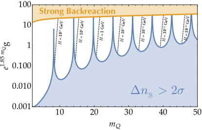
where we ignore the sub-leading backreaction from or . We first estimate these contributions analytically. Using (13) and background relation and changing variables into with the integration domain , one can write , and , where all the ’s approximately follow . For a given value of , these terms would easily dominate (7), (9) and (10) for large , if one took as a free parameter. However, this would infer that strong backreaction prevents the system from reaching such a parameter region. The conditions to ensure that each of and is subdominant in (7), (9) and (10) are translated into upper bounds on ,
| (19) |
where . In Fig. 1, we show the strongest constraints coming from , though they are almost degenerate.
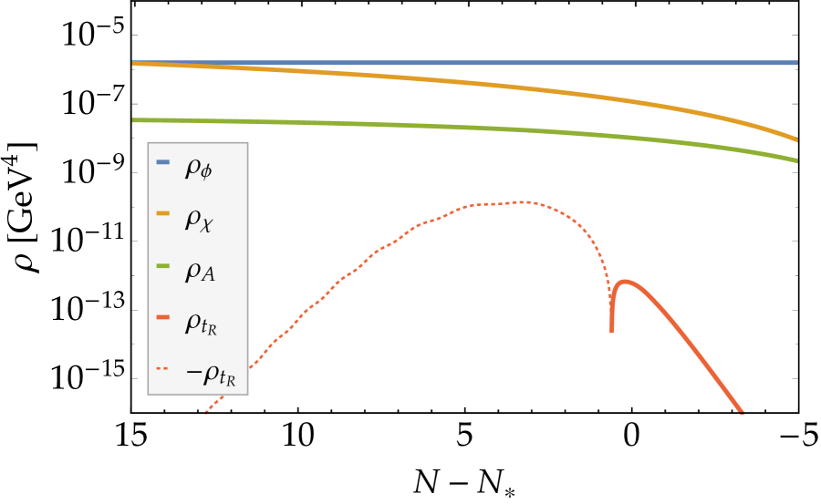
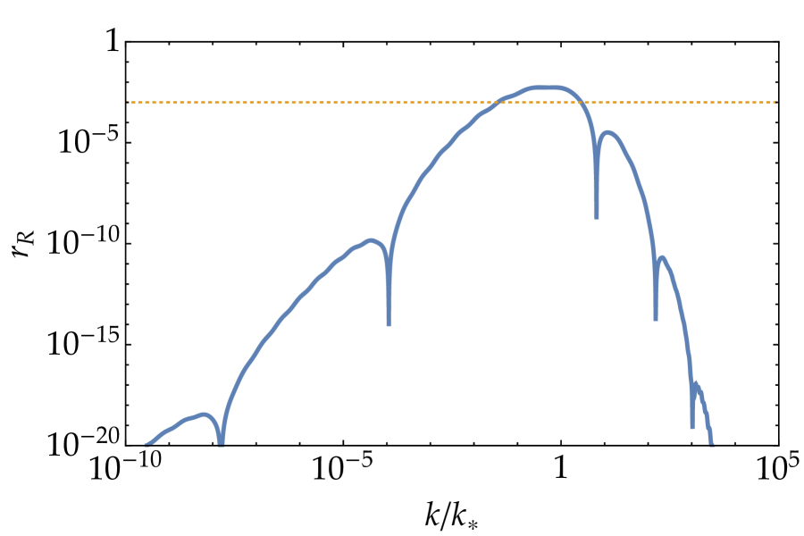
For large , the backreaction is not completely negligible even in the allowed region shown in Fig. 1. In those cases, one has to resort to full numerical calculations simultaneously solving all equations of motion for background fields, (8)–(10) and for perturbations, (11) and (12) with full source terms included. Fig. 2 shows our numerical result for the following parameters:
| (20) |
where the corresponding maximum of is around 44. The tensor-to-scalar ratio where is the pivot scale for CMB observations indeed exceeds the detectable limit even with such a extremely low inflationary energy scale .


|
III.2 B. Curvature Perturbation
Previous attempts to generate GW from scalar or vector fields are tightly constrained by the CMB observation on the curvature perturbation Cook and Sorbo (2012); Ferreira and Sloth (2014); *Ferreira:2015omg. In our model, the inflaton fluctuation is assumed to be responsible for generating compatible with the CMB observation. Contributions from the other scalar modes , and to are negligible, unless becomes a curvaton Dimastrogiovanni et al. (2017).
In addition, we investigate another channel in which the second order effect of produces the inflaton perturbation, , through the gravitational interaction. This effect arises only at the second order due to the absence of linear couplings between and , while the sourcing of to the GW is first-order, thus is expected to be negligible for the parameter range of our interest. We will address this effect in detail in the upcoming work.
Even though the part of sourced by the second order of or the linear order of the scalar perturbations in the axion- sector only has negligible effects, that of originated from its own vacuum fluctuations can be influenced by the background fields and , due to their contribution to . As a result, the spectral index in our model reads,
| (21) |
where in the last step we have used , true with the parameters of our interest. The Planck measures Ade et al. (2016b), and without assuming an accidental cancellation between and , we require a bound on as
| (22) |
where denotes the time of the horizon crossing of the CMB modes. Note that this constraint can be relaxed if is positive. When (22) saturates, in our model, can explain the red-tilted curvature perturbations without a huge hierarchy of slow-roll parameters . It is a quite intriguing possibility for small-field inflationary models since all slow-roll parameters are naively expected to be equivalently small in that class of inflation. We numerically checked that within 2 of Planck constraints is realized solely by for the parameters (III.1).
III.3 C. Perturbativity
Since the amplitude of is substantially amplified due to the instability in our model, we need to ensure that it does not invalidate our perturbative calculation. We thus impose that the -loop contribution to the two-point function should be negligible to that of the tree level. The terms lead to three- and four-point vertices, and it can be shown that their one-loop diagrams give contributions of the same order Ferreira and Sloth (2014). We here focus on the latter and demonstrate that the perturbativity condition gives no additional bounds on the model parameters. The four-point interaction Hamiltonian reads
| (24) |
giving rise to, using the in-in formalism,
| (25) |
where we ignored the left-handed mode. Defining as the ratio of (25) divided by the tree-level contribution, , evaluated at the time when reaches its maximum value, we ensure to safely ignore the higher-order loops and to justify the perturbative approach. Evaluating (25) with (13), we verify that is satisfied up to for .
IV IV. Conclusion
The main message of this Letter is that the detection of primordial gravitational waves does not necessarily exclude low-energy inflation. Once an gauge field has a background configuration that respects the spatial rotation, its perturbations are coupled to the GW at the linear order. The former is amplified by instabilities around the horizon crossing, whose power is then linearly transferred to the latter. We have demonstrated that the GW power spectrum produced from this mechanism can be as significant as at detectable levels respecting all the consistency conditions, even if the inflationary energy scale is close to the BBN bound.
Having a possible alternative source of GW, it is crucial to discriminate the generation mechanism of primordial GW to reveal the true energy scale of inflation. Fortunately, our model has the following distinct predictions to be distinguished from the conventional vacuum GW. (i) The fully parity-violating GW may be detected through CMB temperature and B-mode (TB) or E-mode and B-mode polarization (EB) cross-correlation by the upcoming satellite mission such as LiteBIRD Thorne et al. (tion). (ii) Our model produces a sizable tensor non-Gaussianity with a particular shape Agrawal et al. (tion). (iii) The conventional consistency relation, , is broken, where is the tensor spectral index. With the future observation, these signatures will carry important information for rigorous determination of inflationary energy scale.
V Acknowledgement
We would like to thank Emanuela Dimastrogiovanni, Matteo Fasiello, Shinji Mukohyama, Marco Peloso, Matthew Reece, Martin Sloth, Henry Tye and Yi Wang for useful discussions and correspondences. TF acknowledges the support by Grant-in-Aid for JSPS Fellows No. 29-9103. RN is supported by the Natural Sciences and Engineering Research Council (NSERC) of Canada and by the Lorne Trottier Chair in Astrophysics and Cosmology at McGill University. YT is supported by Japan Society for the Promotion of Science Research Fellowship for Young Scientists and grants from Région Île-de-France.
References
- Kamionkowski et al. (1997) M. Kamionkowski, A. Kosowsky, and A. Stebbins, Phys. Rev. Lett. 78, 2058 (1997), arXiv:astro-ph/9609132 [astro-ph] .
- Seljak and Zaldarriaga (1997) U. Seljak and M. Zaldarriaga, Phys. Rev. Lett. 78, 2054 (1997), arXiv:astro-ph/9609169 [astro-ph] .
- Ade et al. (2016a) P. A. R. Ade et al. (BICEP2, Keck Array), Phys. Rev. Lett. 116, 031302 (2016a), arXiv:1510.09217 [astro-ph.CO] .
- Abazajian et al. (2015) K. N. Abazajian et al., Astropart. Phys. 63, 55 (2015), arXiv:1309.5381 [astro-ph.CO] .
- Ade et al. (2016b) P. A. R. Ade et al. (Planck), Astron. Astrophys. 594, A20 (2016b), arXiv:1502.02114 [astro-ph.CO] .
- Cook and Sorbo (2012) J. L. Cook and L. Sorbo, Phys. Rev. D85, 023534 (2012), [Erratum: Phys. Rev.D86,069901(2012)], arXiv:1109.0022 [astro-ph.CO] .
- Senatore et al. (2014) L. Senatore, E. Silverstein, and M. Zaldarriaga, JCAP 1408, 016 (2014), arXiv:1109.0542 [hep-th] .
- Barnaby et al. (2012) N. Barnaby, J. Moxon, R. Namba, M. Peloso, G. Shiu, and P. Zhou, Phys. Rev. D86, 103508 (2012), arXiv:1206.6117 [astro-ph.CO] .
- Biagetti et al. (2013) M. Biagetti, M. Fasiello, and A. Riotto, Phys. Rev. D88, 103518 (2013), arXiv:1305.7241 [astro-ph.CO] .
- Biagetti et al. (2015) M. Biagetti, E. Dimastrogiovanni, M. Fasiello, and M. Peloso, JCAP 1504, 011 (2015), arXiv:1411.3029 [astro-ph.CO] .
- Fujita et al. (2015) T. Fujita, J. Yokoyama, and S. Yokoyama, PTEP 2015, 043E01 (2015), arXiv:1411.3658 [astro-ph.CO] .
- Mirbabayi et al. (2015) M. Mirbabayi, L. Senatore, E. Silverstein, and M. Zaldarriaga, Phys. Rev. D91, 063518 (2015), arXiv:1412.0665 [hep-th] .
- Adshead and Wyman (2012) P. Adshead and M. Wyman, Phys. Rev. Lett. 108, 261302 (2012), arXiv:1202.2366 [hep-th] .
- Adshead et al. (2013) P. Adshead, E. Martinec, and M. Wyman, JHEP 09, 087 (2013), arXiv:1305.2930 [hep-th] .
- Maleknejad and Erfani (2014) A. Maleknejad and E. Erfani, JCAP 1403, 016 (2014), arXiv:1311.3361 [hep-th] .
- Dimastrogiovanni et al. (2017) E. Dimastrogiovanni, M. Fasiello, and T. Fujita, JCAP 1701, 019 (2017), arXiv:1608.04216 [astro-ph.CO] .
- Dimastrogiovanni et al. (2013) E. Dimastrogiovanni, M. Fasiello, and A. J. Tolley, JCAP 1302, 046 (2013), arXiv:1211.1396 [hep-th] .
- Dimastrogiovanni and Peloso (2013) E. Dimastrogiovanni and M. Peloso, Phys. Rev. D87, 103501 (2013), arXiv:1212.5184 [astro-ph.CO] .
- Ferreira and Sloth (2014) R. Z. Ferreira and M. S. Sloth, JHEP 12, 139 (2014), arXiv:1409.5799 [hep-ph] .
- Ferreira et al. (2016) R. Z. Ferreira, J. Ganc, J. Noreña, and M. S. Sloth, JCAP 1604, 039 (2016), [Erratum: JCAP1610,no.10,E01(2016)], arXiv:1512.06116 [astro-ph.CO] .
- Thorne et al. (tion) B. Thorne, T. Fujita, M. Hazumi, N. Katayama, E. Komatsu, and M. Shiraishi, (in preparation).
- Agrawal et al. (tion) A. Agrawal, T. Fujita, and E. Komatsu, (in preparation).