OGLE-2016-BLG-1003: First Resolved Caustic-crossing Binary-source Event Discovered by Second-generation Microlensing Surveys

Abstract

We report the analysis of the first resolved caustic-crossing binary-source microlensing event OGLE-2016-BLG-1003. The event is densely covered by the round-the-clock observations of three surveys. The light curve is characterized by two nested caustic-crossing features, which is unusual for typical caustic-crossing perturbations. From the modeling of the light curve, we find that the anomaly is produced by a binary source passing over a caustic formed by a binary lens. The result proves the importance of high-cadence and continuous observations, and the capability of second-generation microlensing experiments to identify such complex perturbations that are previously unknown. However, the result also raises the issues of the limitations of current analysis techniques for understanding lens systems beyond two masses and of determining the appropriate multiband observing strategy of survey experiments.

1. Introduction

Since the first microlensing surveys (Alcock et al., 1993; Aubourg et al., 1993; Udalski et al., 1993), the microlensing experiment has achieved remarkable progress through the advent of new observation surveys (e.g., MOA: Sumi et al. 2011, KMTNet: Kim et al. 2016), and the improvement in both software (e.g., improved photometry based on difference imaging) and hardware (e.g., large-format wide-field cameras). As a result, the detection rate of microlensing events, which was several dozen per year in early experiments, is now more about two thousand events per year. In addition, the progress now enables surveys to densely and continuously cover lensing events with a high enough cadence to detect various microlensing signals without follow-up observations.

Dense and continuous coverage of lensing light curves is important for various scientific studies in microlensing. The most prominent example is planetary microlensing events. The lensing signal of a planet generally appears a short-lasting perturbation to a standard Paczyński (1986) curve induced by the host of the planet, and the duration of the signal is on the order of hours for Earth-mass planets and several days for Jupiter-mass planets. Therefore, one would expect that lensing events need to be monitored with a cadence of $\lesssim 1~{}\rm hr^{-1}$ for low-mass planets and of $\lesssim 1~{}\rm day^{-1}$ for giant planets. With the improvement of observational equipment and the development of observational strategy, current-generation experiments are able to monitor large number of lensing events with cadences high enough to detect planets by survey only data (e.g., Udalski et al. 2015c; Sumi et al. 2016; Shin et al. 2016).

Another area that has benefitted from dense and continuous observations is caustic-crossing microlensing events. When a lens is composed of multiple masses, the light curve often exhibits a slope discontinuity. This discontinuity occurs when a source is located at some positions (caustics) at which the point-source magnification diverges (Schneider & Weiss, 1986; Erdl & Schneider, 1993). In addition, if the source passes close to or over the caustic, the different parts of the source are magnified differently, resulting in the deviation from the point-source magnification. Detecting this finite-source effect is important because it provides an opportunity to measure the angular Einstein radius $\theta_{\rm E}$, which makes it possible to better constrain the physical properties of the lens system (Gould, 1994). Despite its importance, the measurement of $\theta_{\rm E}$ is difficult due to the short duration of caustic crossings as well as the difficulty of predicting the time of occurrence. For most caustic-crossing events, the duration of the signal is order of hours. Therefore, resolving the caustic crossings also requires high-cadence observations similar to the cadence for low-mass planets (Shin et al., 2016).

High-cadence and continuity of microlensing observations is also crucial to identify the nature of lensing events. Aside from inherent degeneracies originating in symmetries of the lens-mapping equation itself (e.g., Dominik 1999), one often confronts cases in which different interpretations can explain observed light curves due to the incomplete coverage of the perturbation. For example, Gaudi & Han (2004) showed that sparse coverage of planet-like anomalies can give rise to severe ambiguities in the interpretation. In addition, Park et al. (2014) pointed out that incomplete coverage also causes ambiguity between stellar and planetary interpretations even though the perturbation clearly shows a large deviation from the standard Paczyński curve. Furthermore, Jung et al. (2017) discussed that if the coverage of the anomaly is sparse, binary-source solutions can be confused with planetary solutions in the case of long-term planet-like perturbations.

In this paper, we demonstrate the importance of high-cadence and continuous observations, and the capability of second-generation microlensing experiments by presenting the analysis of the lensing event OGLE-2016-BLG-1003. The event was densely covered by the round-the-clock observations of three surveys including KMTNet, OGLE, and MOA. The light curve exhibits two nested pairs of caustic-crossing features, which is unusual for typical caustic-crossing perturbations.

2. Observation

Figure 1.— Light curve of OGLE-2016-BLG-1003. Two insets show the zoom of the perturbations centered at ${\rm HJD}^{\prime}\sim 7541$ and $7558$, respectively. The notation in the parenthesis represents the observation passband.

The equatorial coordinates of OGLE-2016-BLG-1003 are $(\alpha,\delta)_{\rm J2000}=(17^{\rm h}36^{\rm m}25^{\rm s}\hskip-2.0pt.23,-27^{\circ}11^{\prime}19^{\prime\prime}\hskip-2.0pt.9)$, which correspond to Galactic coordinates $(l,b)=(0.41^{\circ},2.65^{\circ})$. On 2016 June 18, the event was announced by the OGLE group through the Early Warning System (EWS: Udalski et al., 2015b). The OGLE group uses the 1.3m Warsaw telescope at the Las Campanas Observatory in Chile. This field was independently monitored by the MOA survey with its 1.8m telescope at Mt. John Observatory in New Zealand.

The lensed star was also in the fields of the KMTNet survey, which consists of three identical 1.6m telescopes equipped with a $4.0~{}\rm deg^{2}$ mosaic camera that are located at the Cerro Tololo Inter-American Observatory in Chile (KMTC), South African Astronomical Observatory in South Africa (KMTS), and Siding Spring Observatory in Australia (KMTA). With these wide-field telescopes that are globally distributed, the survey continuously observed the event with $\sim 1~{}\rm hr^{-1}$ cadence.

Table 1Correction Parameters

Observatory	Number	$k$	$\sigma_{\rm min}$ (mag)
OGLE $(I)$	1716	1.587	0.005
MOA $(RI)$	749	0.905	0.001
KMTC $(I)$	791	0.922	0.001
KMTS $(I)$	693	0.995	0.001
KMTA $(I)$	290	1.077	0.003
KMTC $(V)$	41	1.068	0.001
KMTS $(V)$	20	1.015	0.001

Figure 2.— Light curves of 1S3L and 2S2L interpretations without the MOA data. The curve with cyan color is the best-fit 1S3L solution, while the two curves with orange and black colors are the best-fit 2S2L solutions for $V$ and $I$ band, respectively. The two insets show the zoom of the perturbations near ${\rm HJD}^{\prime}\sim 7541$ and $7558$.

Data reduction was performed by the individual survey groups using their customized pipelines. All of these pipelines are developed based on the image subtraction technique (Alard & Lupton, 1998). In order to use the data sets acquired from the different photometry codes, we readjust the error bars of each data set using the standard method in microlensing (Yee et al., 2012). Based on the error derived from the pipeline, $\sigma_{0}$, the remormalized error is calculated by

$$\sigma^{\prime}=\sqrt{\sigma_{\rm min}^{2}+(k\sigma_{0})^{2}}.$$ (1)

Here $\sigma_{\rm min}$ is a factor needed to adjust the error to be consistent with the scatter of the data, and $k$ is a scaling factor needed to make $\chi^{2}/{\rm dof}\sim 1$. In Table 1, we list the values of the error parameters for each data set with the total number of data and the observing passband.

3. Analysis

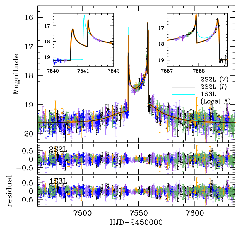
The OGLE-2016-BLG-1003 light curve (Figure 1) shows a large U-shaped brightness variation, suggesting that the event seems to be a typical binary-lens event characterized by a caustic entrance followed by a caustic exit. However, dense and continuous observations reveal that the light curve exhibits four distinctive spikes that occurred at ${\rm HJD}^{\prime}(={\rm HJD}-2,450,000)\sim 7540.9,7541.2,7557.9$, and $7558.6$. Such complex deviations are unusual for typical caustic-crossing perturbations.

In fact, the MOA data remained unreduced until we encountered a degeneracy between two interpretations as presented below. Although one of these was proved to be incorrect from the MOA data, examining the degeneracy is very important because (1) it raises the issue of the limitations of current analysis techniques for understanding lens systems beyond two masses (i.e., triple-lens system), and (2) it provides an opportunity for pondering the observational strategy of future microlensing experiments. Therefore, we first study the event without the MOA data.

3.1. Without MOA data

Figure 3.— Geometries of 1S3L and 2S2L interpretations without the MOA data. In each panel, the closed curve represents the caustic, and the line with an arrow is the source trajectory. The locations of the lens components are represented by the blue filled circles. The right panels show the enlarged view of the left panel corresponding to the anomaly region near ${\rm HJD}^{\prime}\sim 7558$. In the case of the 1S3L solutions, the positions of lens component and caustic change in time due to the orbital motion. We show three sets of caustics at ${\rm HJD}^{\prime}\sim 7540$, $7550$, and $7560$. All lengths are normalized to the Einstein radius $\theta_{\rm E}$.

To explain the light curve, we initially search for the solution based on a single-source binary-lens (1S2L) interpretation. Using the parametrization and the method of Jung et al. (2015), we investigate the parameter space considering higher-order effects such as lens orbital motion (Dominik, 1998) and microlens parallax (Gould, 1992, 2004). However, because of the two distinct features at ${\rm HJD}^{\prime}\sim 7557.9$ and $7558.6$, we could not find a satisfactory model describing the perturbations. We therefore take into account two additional interpretations that have a possibility to cause such complex deviations. The first interpretation is that the lens is composed of three masses (1S3L) and the second is that both the source and the lens contain two components (2S2L).

3.1.1 Single-source Triple-lens Modeling

The 1S3L modeling is conducted using a similar method to that of Udalski et al. (2015a) and Bennett et al. (2017). First, we search for the 1S2L parameters that describe the dominant U-shaped anomaly by removing the data around ${\rm HJD}^{\prime}\sim 7558.6$. We then recover the data and perform an additional grid search over $(s_{2},q_{2},\psi)$ space by fixing the $(s_{1},q_{1})$ parameters, where $s_{1}$ (normalized to $\theta_{\rm E}$) is the projected binary separation and $q_{1}=M_{2}/M_{1}$. Here $s_{2}$ (normalized to $\theta_{\rm E}$) is the projected separation between the third mass $M_{3}$ and the barycenter of the binary lens $({\rm CM_{B}})$, $\psi$ is the angle between the ${\rm CM_{B}}-M_{3}$ axis and the binary-lens axis, and $q_{2}=M_{3}/M_{1}$. We note that the grid parameters $(s_{1},q_{1},s_{2},q_{2},\psi)$ are fixed during the computation, while other parameters are allowed to vary from their initial values. Finally, to refine each local minimum, we seed a Markov Chain Monte Carlo (MCMC) with its parameters, and allow all of these to vary.

Table 2Best-fit Parameters

Parameters	Without MOA data					With MOA data
	1S3L				2S2L	2S2L
	Local A		Local B			Without Prior	With Prior
	Standard	Orbit+Parallax	Standard	Orbit+Parallax	Standard	Standard	Standard
$\chi^{2}$/dof	3604.2/3541	3530.9/3535	3610.7/3541	3531.8/3535	3531.3/3539	4288.1/4288
$t_{0,1}$ (HJD′)	7551.978$\pm$0.135	7552.916$\pm$0.137	7551.928$\pm$0.123	7552.931$\pm$0.153	7551.038$\pm$0.204	7549.825$\pm$0.182	7549.977$\pm$0.094
$u_{0,1}$	0.092$\pm$0.004	-0.125$\pm$0.005	0.092$\pm$0.003	-0.124$\pm$0.004	0.059$\pm$0.013	-0.022$\pm$0.010	-0.015$\pm$0.007
$t_{0,2}$ (HJD′)	–	–	–	–	7552.517$\pm$0.134	7553.146$\pm$0.129	7553.256$\pm$0.107
$u_{0,2}$	–	–	–	–	0.135$\pm$0.006	0.135$\pm$0.004	0.134$\pm$0.003
$t_{\rm E}$ (days)	39.832$\pm$1.415	31.971$\pm$1.056	40.216$\pm$1.345	33.334$\pm$1.030	28.931$\pm$0.665	29.860$\pm$0.632	30.203$\pm$0.649
$s_{1}$	0.954$\pm$0.014	1.066$\pm$0.013	0.948$\pm$0.013	1.042$\pm$0.014	1.033$\pm$0.011	1.014$\pm$0.010	1.006$\pm$0.011
$q_{1}$	0.248$\pm$0.013	0.232$\pm$0.011	0.249$\pm$0.012	0.217$\pm$0.014	1.188$\pm$0.039	1.407$\pm$0.013	1.428$\pm$0.014
$\alpha$ (rad)	2.554$\pm$0.015	-2.652$\pm$0.016	2.551$\pm$0.013	-2.654$\pm$0.018	0.842$\pm$0.015	0.875$\pm$0.014	0.893$\pm$0.012
$s_{2}$	0.941$\pm$0.011	0.944$\pm$0.021	0.786$\pm$0.011	0.937$\pm$0.021	–	–	–
$q_{2}$ $(10^{-3})$	1.054$\pm$0.162	1.256$\pm$0.158	1.082$\pm$0.192	1.176$\pm$0.251	–	–	–
$\psi$ (rad)	1.594$\pm$0.028	-1.538$\pm$0.043	1.615$\pm$0.032	-1.377$\pm$0.051	–	–	–
$\rho_{*,1}$ $(10^{-3})$	0.603$\pm$0.058	0.685$\pm$0.062	0.553$\pm$0.056	0.570$\pm$0.060	$0.451_{-0.121}^{+1.422}$	1.003$\pm$0.351	1.321$\pm$0.048
$\rho_{*,2}$ $(10^{-3})$	–	–	–	–	1.293$\pm$0.161	1.371$\pm$0.068	1.368$\pm$0.053
$\pi_{{\rm E},N}$	–	-0.614$\pm$0.423	–	-0.585$\pm$0.367	–	–	–
$\pi_{{\rm E},E}$	–	0.382$\pm$0.153	–	0.603$\pm$0.110	–	–	–
$ds_{1}/dt$ $({\rm yr}^{-1})$	–	-3.342$\pm$0.122	–	-3.229$\pm$0.120	–	–	–
$d\alpha/dt$ $({\rm yr}^{-1})$	–	1.273$\pm$0.179	–	1.191$\pm$0.204	–	–	–
$ds_{2}/dt$ $({\rm yr}^{-1})$	–	-0.498$\pm$0.373	–	-3.526$\pm$0.405	–	–	–
$d\psi/dt$ $({\rm yr}^{-1})$	–	1.500$\pm$0.443	–	-1.515$\pm$0.513	–	–	–
$q_{F,V}$	–	–	–	–	1.202$\pm$0.201	1.047$\pm$0.234	1.070$\pm$0.036
$q_{F,RI}$	–	–	–	–	–	0.981$\pm$0.032	1.033$\pm$0.031
$q_{F,I}$	–	–	–	–	1.182$\pm$0.054	1.037$\pm$0.037	1.068$\pm$0.036

Note. — ${\rm HJD}^{\prime}={\rm HJD}-2450000$

We find that two degenerate 1S3L models (marked as “A” and “B”) can explain the light curve. However, there are some residuals in both solutions. This triggers the further investigation considering both the parallax and the lens orbital effect (“orbit+parallax”). Accounting for the parallax effect requires including two additional parameters ${\mbox{\boldmath$\pi$}}_{\rm E}=(\pi_{\rm E,\it N},\pi_{\rm E,\it E})$, which are the vector components of the microlens parallax (Gould, 2004). For the consideration of the orbital effects, we include four additional parameters $(ds_{1}/dt,d\alpha/dt,ds_{2}/dt,d\psi/dt)$, which describe, respectively, the change rate of $s_{1}$, $\alpha$, $s_{2}$, and $\psi$ to first-order approximation. When we test the model with these higher-order effects, we test $u_{0}>0$ and $u_{0}<0$ solutions to consider the “ecliptic degeneracy” (Jiang et al., 2004; Skowron et al., 2011). We note that because the third mass is much smaller than the other two masses, we adopt ${\rm CM_{B}}$ as a reference position of the lens system.

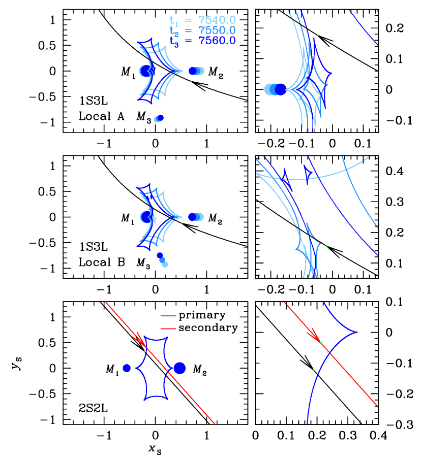
In Table 2, we present the two solutions. The best-fit model light curve (local A) is shown in Figure 2. The lensing geometries of the individual solutions are presented in the upper and middle panels of Figure 3. We find that the light curve is generated by a circumbinary planet orbiting a stellar binary. The perturbations near ${\rm HJD}^{\prime}\sim 7541.2$ and $7558.6$ are produced by the source crossing over the resonant caustic formed by the binary lens, while the perturbation near ${\rm HJD}^{\prime}\sim 7557.9$ is produced by the source passing close to the central caustic induced by the planet located near the Einstein ring. Although the two solutions cause ambiguity in the $s_{2}$ measurement, the two mass ratios $q_{1}$ and $q_{2}$ are almost same in both solutions.

3.1.2 Binary-source Binary-lens Modeling

The binary-source lensing magnification is described by the flux-weighted mean of two single-source magnifications, i.e., $A=(A_{1}F_{1}+A_{2}F_{2})/(F_{1}+F_{2})$, where $F_{i}$ and $A_{i}$ denote the flux and magnification of the individual sources (Griest & Hu, 1992). The single-source magnification is related to the lens mapping from the source plane to the image plane, resulting in the distortion of images. The lens-mapping equation is represented by

$$\zeta=z-\sum_{i=1}^{N_{l}}{\epsilon_{i}\over\bar{z}-\bar{z}_{m,i}},$$ (2)

where $N_{l}$ is the number of lens components, $\epsilon_{i}=m_{i}/M_{\rm tot}$, and $M_{\rm tot}$ is the total mass of the lens system. Here $\zeta$, $z_{m,i}$, and $z$ are, respectively, the positions of the source, lens components, and images in complex coordinates, and the bar denotes the complex conjugate. Note that all angles are normalized to $\theta_{\rm E}$. The magnification $A_{j}$ of jth image is then determined from the amount of the distortion of the image given by the inverse of the determinant of the Jacobian, i.e.,

$$A_{j}={1\over\left|{\rm det}J\right|};\qquad{\rm det}J=\left.{1-{\partial\zeta\over\partial\bar{z}}{\partial\bar{\zeta}\over\partial z}}\right|_{z=z_{j}},$$ (3)

and the single-source magnification is thus the sum of all magnified images $A=\sum_{j}A_{j}$.

For the interpretation of the light curve, we define the principal 2S2L lensing parameters with the approximation that the relative motion between the lens and each source star is rectilinear, and the trajectories of two sources are parallel each other. Based on the 1S2L parametrization, the description of a standard 2S2L light curve then requires 4 additional parameters related to the additional source companion: $(t_{0,2},u_{0,2},\rho_{*,2},q_{F})$. Here the definitions of $(t_{0,2},u_{0,2})$ are the same as those for a single-source single-lens event, $\rho_{*,2}$ is the source radius of the second source, and $q_{F}=F_{2}/F_{1}$ is the flux ratio between the two sources, which is needed to compute the individual source fluxes. We note that the flux ratio depends on the passband (Griest & Hu, 1992; Hwang et al., 2013; Jung et al., 2017), and thus one should allot separate $q_{F}$ parameters to each observed passband.

Figure 4.— $\Delta\chi^{2}$ distribution in $(s,q)$ space obtained from the 2S2L grid search. Each color represents the point of the space within $1n\sigma$ (red), $2n\sigma$ (yellow), $3n\sigma$ (green), $4n\sigma$ (light blue), $5n\sigma$ (blue), and $6n\sigma$ (purple) level from the best-fit solution, where $n=20$.

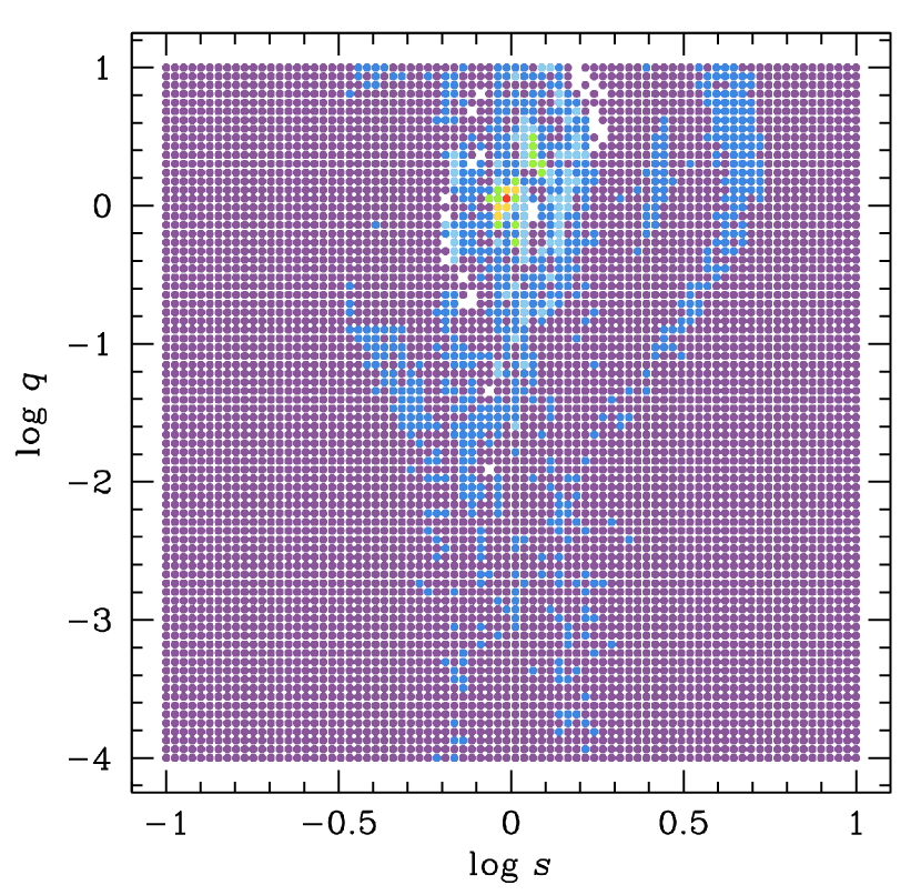
We search for the 2S2L solution using a method similar to Jung et al. (2015). We first perform an initial grid search. We set $s$, $q$, $\alpha$, and $q_{F}$ as grid parameters since the lensing magnification varies sensitively to the change of these parameters, while the magnification varies smoothly to the changes of the other parameters. The grid parameters $(s,q,\alpha,q_{F})$ are divided by $(80,80,11,11)$ grids and span the range of $-1.0<{\rm log}~{}s<1.0$, $-4.0<{\rm log}~{}q<1.0$, $0<{\alpha}<2\pi$, and $-5.0<{\rm log}~{}q_{F}<5.0$, respectively. At each grid point, we use the fixed value of $(s,q)$, while we allow $\alpha$ and $q_{F}$ to vary during the computation. Here we assume that the flux ratio is same for all passbands because the difference of magnification between different $q_{F}$ parameters is quite subtle compared to that of other parameters. Figure 4 shows the $\Delta\chi^{2}$ distribution in the $(s,q)$ space obtained from this initial search. It clearly shows that there is only one local minimum. We then assign individual $q_{F}$ parameters to individual passbands, and find a best-fit solution from further refinement of the local solutions.

We find that the 2S2L solution also gives an excellent fit to the complex perturbations. In Table 2, we list the best-fit parameters. The model light curve is presented in Figure 2. We show two model curves corresponding to each observed passband because the binary-source magnification is wavelength dependent. In Figure 3, we present the lensing geometry (lower panel) in which the two source trajectories are separately illustrated by a straight line with arrow head. We note that the source approaching closer to the barycenter of the lens is marked as the “primary” and the other source is marked as the “secondary”. According to the 2S2L solution, the outer and inner pair of caustic-crossing features are produced by the secondary and the primary source passing over the resonant caustic, respectively.

Figure 5.— Enlarged view of the light curve around the caustic-crossing perturbations. The three curves with orange, red, and black colors are the best-fit models for $V$, $RI$ and $I$ bands. They are nearly indistinguishable. The caustic entrance and the exit formed by the primary and the secondary source are marked by “1” and “2”, respectively.

From the comparison between the 1S3L and the 2S2L interpretations, we find that both interpretations almost equally well describe the observed light curve. The $\chi^{2}$ difference between two solutions is $\Delta\chi^{2}<1$, indicating that they are extremely degenerate. The similarity of the fits notwithstanding, the two models predict very different brightening variation near ${\rm HJD}^{\prime}\sim 7541$: one caustic entrance for 1S3L model and two caustic entrances for 2S2L model. As a result, one could distinguish the two interpretations if there exist data points with a cadence high enough to identify such characteristic features.

3.2. With MOA data

The degeneracy seemed to remain unresolved. However, it was noticed that the event was also in one of the MOA observation fields, although it was not registered in the MOA event list. In addition, it was immediately recognized that the MOA data could play an important role to distinguish the degeneracy because the time zone of the MOA site exactly matched the unresolved part of the light curve.

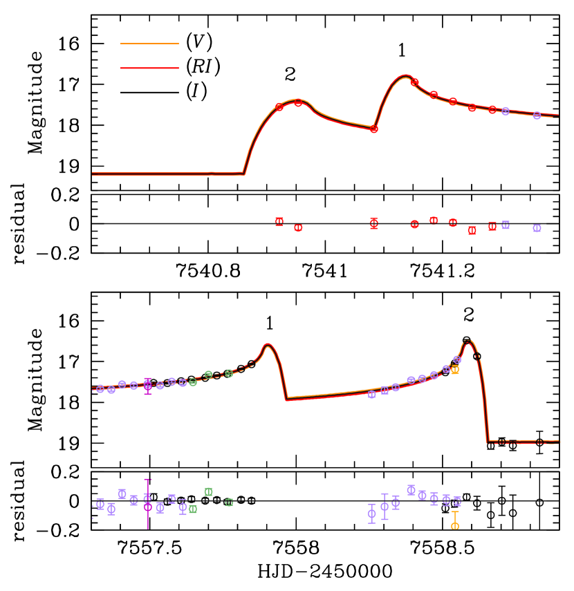
We find that the MOA survey covers the unresolved region in which the data clearly show the feature of two caustic entrances. It definitively supports the 2S2L interpretation. With the MOA data, we further refine the 2S2L solution. The best-fit parameters are listed in Table 2. In Figure 5, we present the light curve of the 2S2L solution in the caustic-crossing region. Since the overall light curve and the lensing geometry are almost same as those derived without the MOA data, we do not present these redundant figures. The estimated flux ratios $(q_{F,V},q_{F,RI},q_{F,I})=(1.05,0.98,1.04)$ are very close to unity, implying that the brightness of the two sources is quite similar. This resemblance consequently indicates that the two sources would have similar $\rho_{*,i}$ values. However, unfortunately, we find that $\rho_{*,1}$ is not well constrained; it has a range of $0<\rho_{*,1}<0.0014$ due to the sparse coverage of the caustic crossing corresponding to the primary source (see Figure 5).

Figure 6.— Positions of individual source stars in the instrumental color magnitude diagram of nearby stars. Also shown is the position of the giant clump centroid.

To check the result that comes from the poorly constrained $\rho_{*,1}$, we test an additional model including a physical constraint. One important characteristic of the 2S2L interpretation is that the measured $\theta_{\rm E,\it i}$ from the individual source radii $\rho_{*,i}$ must be consistent each other. Following this argument, we impose the gaussian constraint,

$$f(\theta_{\rm E,1})\sim e^{-(\theta_{\rm E,1}-\theta_{\rm E,2})^{2}/\sigma_{\rm E,2}^{2}},$$ (4)

on the MCMC chains by adopting the error of $\theta_{\rm E}$ as $\sigma_{\rm E,2}$ (see next section). For the measurement of $\theta_{\rm E,\it i}$, we include the KMTC DoPhot $I$ and $V$ band data solely to obtain their flux fraction by fitting along with other data sets. As presented in the seventh and eighth columns of Table 2, we find that the derived parameters are almost consistent and the prior does not affect the precision of the parameters significantly. In addition, the measured $\rho_{*,2}$ from both solutions are almost exactly same, indicating that the derived $\theta_{\rm E}$ is also consistent within the uncertainty level $\sigma_{\rm E}$. Therefore, we use the result to characterize the two source stars.

3.3. Source Type

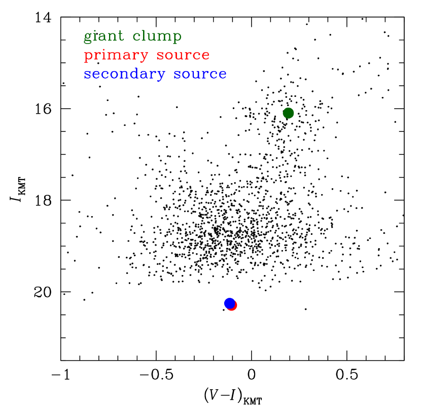
We determine the source type by following the procedure of Yoo et al. (2004). We first identify the individual source positions in the instrumental color-magnitude diagram (see Figure 6). We next measure the offsets $\Delta(V-I,I)$ between the giant clump centroid (GC) and the individual sources. From the de-reddened brightness $I_{0,\rm GC}=14.43$ (Nataf et al., 2013) and color $(V-I)_{0,\rm GC}=1.06$ (Bensby et al., 2011) of GC, we then estimate the de-reddened brightness $I_{0}$ and color $(V-I)_{0}$ of each source star. Here we assume that the GC and the source experience identical extinction. The derived $(V-I,I)_{0,i}$ of the two sources are $(V-I,I)_{0,1}=(0.76\pm 0.13,18.63\pm 0.05)$ and $(V-I,I)_{0,2}=(0.75\pm 0.12,18.59\pm 0.05)$, respectively. These indicate that the binary source is composed of two G-type main sequence stars.

Since we measure the finite size of the secondary source $\rho_{*,2}$, we also determine the angular Einstein radius $\theta_{\rm E}$. We first convert $(V-I)_{0,i}$ into $(V-K)_{0,i}$ using the $VIK$ color-color relation (Bessell & Brett, 1988), and then deduce the angular size of each source star $\theta_{*,i}$ from the relation between $(V-K)_{0}$ and $\theta_{*}$ (Kervella et al., 2004). The derived angular radii of the individual sources are $(\theta_{*,1},\theta_{*,2})=(0.629\pm 0.045,0.634\pm 0.045)$ $\mu$as. The angular Einstein radius is thus

$$\theta_{\rm E}={\theta_{*,2}\over\rho_{*,2}}=0.462\pm 0.043~{}{\rm mas},$$ (5)

and the proper motion of the binary source relative to the binary lens is

$$\mu={\theta_{\rm E}\over t_{\rm E}}=5.654\pm 0.521~{}{\rm mas~{}yr^{-1}}.$$ (6)

4. Discussion

We have presented an analysis of the event OGLE-2016-BLG-1003 for which the light curve exhibits two pairs of caustic-crossing perturbations. From the analysis considering two different interpretations based on high-cadence and continuous data taken by three microlensing surveys, we found that the anomalies can be explained by the 2S2L model. Our 1S3L models were clearly disfavored by the MOA data. However, the analysis of the event and the process of reaching the conclusion that the 2S2L model is correct demonstrate the potential difficulties of interpreting such complex events.

First, our result does not fully guarantee that the 1S3L interpretation is not the solution, because we only searched a subset of 1S3L parameter space as described in Section 3.1.1. In fact, it is extremely difficult or almost impossible with our current level of understanding to conduct the full 1S3L analysis since current computing power is not even sufficient to obtain the initial solution by setting $(s_{1},q_{1},\alpha,s_{2},q_{2},\psi)$ as independent parameters. Therefore, in most cases, the 1S3L modeling has been done by following a hybrid approach that has been commonly used in this field. This approach is quite reasonable provided that the perturbation induced by the additional lens component does not affect the overall light curve (e.g., planetary perturbation). For example, Udalski et al. (2015a) found the 1S3L solution by first estimating the principal binary-lens parameters that explain the overall light curve, and then by adding the third mass to fit the planet-like perturbation similar to the approach used here. Experience from these events indicates that applying this approach to possible 1S3L candidates is extremely difficult if we could not first find the principal binary-lens parameters. Furthermore, even though the method can provide a plausible model for the light curve, there is no guarantee (i.e., $\Delta\chi^{2}$ surface) that the solution is the global minimum, and unfortunately this issue still remains an open question.

Our result also introduces degeneracy between 1S3L and 2S2L interpretations that can describe the unusual “nested caustics” features (i.e., two caustic entrances or two caustic exits in a row). Although the event reported here favors the 2S2L interpretation, discriminating between them was only possible because we had high-cadence data and the two solutions predicted different lensing magnification curves, which will not always be the case. Nevertheless, it is possible to discriminate between 1S3L and 2S2L solutions due to the different origin of the lensing magnification. As already proven by analyzing observed events (Hwang et al., 2013; Jung et al., 2017), the binary-source magnification depends on the observing passband, and thus one can distinguish between two interpretations with multiband observations.

Until now, however, the major purpose of multiband observations from survey experiments was to determine the source color. Consequently, the observation cadence of the extra passband is much sparser than the primary passband. For example, the ratio between $V$ and $I$ band observations of KMTNet in 2016 was $1/11$ for CTIO site and $1/21$ for SAAO site. Although this cadence is high enough to obtain the source color, we found that it is insufficient to precisely estimate the flux ratio $q_{F,V}$ (see Table 2), which yields the large uncertainty in the $V$ band magnification. As a result, it was difficult to identify the difference of the magnification between different passbands.

With second-generation experiments, we are now able to see many examples of complex perturbations such as reported here, and thus multiband observations become much more important to derive the correct solution. The microlensing event OGLE-2016-BLG-1003 proves the capability of current surveys to identify complex perturbations that are previously unknown. However, it also raises the issues of the limitation of current analysis and determining the appropriate multiband observing strategy of survey experiments.

References

- Alard & Lupton (1998) Alard, C., & Lupton, Robert H. 1998, ApJ, 503, 325
- Alcock et al. (1993) Alcock, C., Akerlof, C. W., Allsman, R. A., et al. 1993, Nature, 365, 621
- Aubourg et al. (1993) Aubourg, E., Bareyre, P., Bréhin, S., et al. 1993, Nature, 365, 623
- Bennett et al. (2017) Bennett, D. P., Rhie, S. H., Udalski, A., et al. 2017, AJ, 152, 125
- Bensby et al. (2011) Bensby, T., Adén, D., Meléndez, J., et al. 2011, A&A, 533, 134
- Bessell & Brett (1988) Bessell, M. S., & Brett, J. M. 1988, PASP, 100, 1134
- Dominik (1998) Dominik, M. 1998, A&A, 329, 361
- Dominik (1999) Dominik, M. 1999, A&A, 349, 108
- Erdl & Schneider (1993) Erdl, H., & Schneider, P. 1993, A&A, 268, 453
- Gaudi & Han (2004) Gaudi, B. S., & Han, C. 2004, ApJ, 611, 528
- Gould (1992) Gould, A. 1992, ApJ, 392, 442
- Gould (1994) Gould, A. 1994, ApJ, 421, L71
- Gould (2004) Gould, A. 2004, ApJ, 606, 319
- Gould & Andronov (1999) Gould, A., & Andronov, N. 1999, ApJ, 516, 236
- Griest & Hu (1992) Griest, K., & Hu, W. 1992, ApJ, 397, 362
- Hwang et al. (2013) Hwang, K.-H., Choi, J.-Y., Bond, I. A., et al. 2013, ApJ, 778, 55
- Jiang et al. (2004) Jiang, G., DePoy, D. L., Gal-Yam, A., et al. 2004, ApJ, 617, 1307
- Jung et al. (2015) Jung, Y. K., Udalski, A., Sumi, T., et al. 2015, ApJ, 798, 123
- Jung et al. (2017) Jung, Y. K., Udalski, A., Yee, J. C., et al. 2017, AJ, 153, 129
- Kervella et al. (2004) Kervella P., Thévenin F., Di Folco E., Ségransan D., 2004, A&A, 426, 297
- Kim et al. (2016) Kim, S.-L., Lee, C.-U., Park, B.-G., et al. 2016, JKAS, 49, 37
- Nataf et al. (2013) Nataf, D. M., Gould, A., Fouqué, P., et al. 2013, ApJ, 769, 88
- Paczyński (1986) Paczyński, B. 1986, ApJ, 304, 1
- Park et al. (2014) Park, H., Han, C., Gould, A., 2014, ApJ, 787, 71
- Schechter et al. (1993) Schechter, P. L., Mateo, M., & Saha, A. 1993, PASP, 105, 1342
- Schneider & Weiss (1986) Schneider, P., & Weiss, A. 1986, A&A, 164, 237
- Shin et al. (2016) Shin, I.-G., Ryu, Y. H., Udalski, A., et al. 2016, JKAS, 49, 73
- Skowron et al. (2011) Skowron, J., Udalski, A., Gould, A., et al. 2011, ApJ, 738, 87
- Sumi et al. (2011) Sumi, T., Kamiya, K., Bennett, D. P., et al. 2011, Nature, 473, 349
- Sumi et al. (2016) Sumi, T., Udalski, A., Bennett, D. P., et al. 2016 ApJ, 825, 112
- Udalski et al. (1993) Udalski, A., Szymanski, M., Kaluzny, J., et al. 1993, Acta Astron., 43, 28
- Udalski et al. (2015a) Udalski, A., Jung, Y. K., Han, C., et al. 2015a ApJ, 812, 47
- Udalski et al. (2015b) Udalski, A., Szymański, M. K., & Szymański, G. 2015b, Acta Astron, 65, 1
- Udalski et al. (2015c) Udalski, A., Yee, J. C., Gould, A., et al. 2015c, ApJ, 799, 237
- Yee et al. (2012) Yee, J. C., Shvartzvald, Y., Gal-Yam, A., et al. 2012, ApJ, 755, 102
- Yoo et al. (2004) Yoo, J., DePoy, D. L., Gal-Yam, A., et al. 2004, ApJ, 603, 139