Population protocols for leader election and exact majority with $O(\log^{2}n)$ states and $O(\log^{2}n)$ convergence time

Abstract

We consider the model of population protocols, which can be viewed as a sequence of random pairwise interactions of $n$ agents (nodes). During each interaction, two agents $v$ and $w$, selected uniformly at random, update their states on the basis of their current states, and the whole system should in long run converge towards a desired global final state. The main question about any given population protocol is whether it converges to the final state and if so, what is the convergence rate.

In this paper we show population protocols for two problems: the leader election and the exact majority voting. The leader election starts with all agents in the same initial state and the goal is to converge to the (global) state when exactly one agent is in a distinct state $L$. The exact majority voting starts with each agent in one of the two distinct states $A$ or $B$ and the goal is to make all nodes know which of these two states was the initial majority state, even if that majority was just by a single vote.

Doty and Soloveichik [DISC 2015] showed that any population protocol for leader election requires expected linear (parallel) time, defined as the number of interactions divided by $n$, if agents have only constant number of states. Alistarh and Gelashvili [ICALP 2015] showed a leader-election protocol which converges in $O(\log^{3}n)$ time w.h.p. and in expectation and needs $\Theta(\log^{3}n)$ states per agent. We present a protocol which elects the leader in $O(\log^{2}n)$ time w.h.p. and in expectation and uses $\Theta(\log^{2}n)$ states per agent. For the exact majority voting, we show a population protocol with the same asymptotic performance: $O(\log^{2}n)$ time and $\Theta(\log^{2}n)$ states per agent. The exact-majority protocol proposed by Alistarh et al. [PODC 2015] achieves expected $O(\log^{2}n)$ time, but requires either the initial imbalance between $A$’s and $B$’s of $\Omega(n/polylog\,n)$ or $\Omega(n/\log n)$ states per agent. (Their protocol can achieve also $O(\log n)$ time, but with $\Omega(n)$ states per agent.) More recently, Alistarh et al. [SODA 2017] showed $O(\log^{2}n)$-state protocols for both problems, with the exact majority protocol converging in time $O(\log^{3}n)$ w.h.p. and in expectation, and the leader election protocol converging in time $O(\log^{6.3}n)$ w.h.p. and $O(\log^{5.3}n)$ in expectation.

Our leader election and exact majority protocols are based on the idea of agents counting their local interactions and rely on the probabilistic fact that the uniform random selection would limit the divergence of the individual counts.

1 Introduction

We consider population protocols [5] for leader election and exact majority voting. A population protocol specifies how two agents, or nodes, change their states when they interact. The computation of a protocol is a (perpetual) sequence of interactions between two nodes. The system consists of $n$ nodes and a scheduler which keeps selecting pairs of nodes for interaction. The objective is that the whole system eventually stabilizes in (converges to) a configuration which has some desired target property. In the general case, the nodes can be connected according to a specified graph $G=(V,E)$ and two nodes can interact only if they are joined by an edge. Following the scenario considered in the majority of previous work on population protocols, we assume the complete communication graph and the random uniform scheduler. That is, each pair of nodes has equal probability to be selected for interaction in the current step, independently of the previous interactions.

The leader election starts with all nodes in the same initial state and the goal is that the system converges to a configuration with exactly one agent in a state which indicates that this node is the leader. The (two-opinion) exact majority voting starts with each node in one of two distinct states $q_{A}$ and $q_{B}$, representing two distinct opinions (or votes) $A$ and $B$. Initially $a_{0}$ nodes hold opinion $A$ (are in the state $q_{A}$) and $b_{0}$ nodes hold opinion $B$, and we assume that $a_{0}\neq b_{0}$. We denote the initial imbalance between the two opinions by $\epsilon=|a_{0}-b_{0}|/n\geq 1/n$. The goal is that eventually all nodes will have the opinion of the initial majority. The exact majority voting should guarantee the correct answer even if the difference between $a_{0}$ and $b_{0}$ is only $1$.

Let $S$ denote the set of states of a population protocol. While $|S|$ can grow with the size $n$ of the population, keeping the number of states low is one of the primary objectives in design of population protocols. Let $q(v,t)\in S$ denote the state of a node $v\in V$ at step $t$ (that is, after $t$ individual interactions). Nodes change their states in pairwise interactions according to a common deterministic transition function $\delta:S\times S\rightarrow\,S\times S$. A population protocol has also an output function $\gamma:S\rightarrow\,\Gamma$, which indicates the property to which the system should converge. For the exact majority voting, $\gamma:S\rightarrow\,\{A,B\}$, which means that a node $v\in V$ in state $q\in S$ assumes that $\gamma(q)$ is the majority opinion. An exact-majority protocol should eventually reach a step $t$, such that for each $v\in V$, $\gamma(q(v,t))$ is the initial majority opinion, and maintain this property in all subsequent steps. For leader election protocols, the output function is $\gamma:S\rightarrow\,\{L,F\}$. A node $v$ in a state $q$ assumes that it is the leader, if $\gamma(q)=L$, or a ’follower,’ if $\gamma(q)=F$.

We consider undirected individual communications, that is, the two interacting nodes are not designated as initiator and responder, so the transition functions must be symmetric. We follow the common convention of defining the (parallel) time as the number of steps (individual interactions) divided by $n/2$, that is, as the average number of interactions per node.

The completion (convergence) time) of a protocol is a random variable $T_{C}$ denoting the (parallel) time when the system stabilizes on the desired property. We are interested in designing protocols for which $T_{C}$ is small w.h.p. $\mathbf{E}(T_{C})$ is finite and ideally also small. A finite $\mathbf{E}(T_{C})$ implies that a protocol cannot stabilize on an incorrect answer with any non-zero probability (even if it was exponentially small in the size of the population). We note that, for example, the pull voting [1, 10] and the two-sample voting [11] do not have this property because of the positive probability that the minority opinion wins. In addition to the analysis of correctness of a given protocol, we also want to derive bounds on the completion time, w.h.p. and/or in expectation. The aim is to achieve fast completion time with small number of states.

1.1 Previous work

Draief and Vojnović [13] and Mertzios et al. [15] analysed two similar four-state exact-majority protocols. Both protocols are based on the idea that the two opinions have “passive/weak” versions $a$ and $b$ and “dynamic/strong” versions $A$ and $B$. The strong versions of opinions can be viewed as tokens moving around the graph. Initially each node $v$ has a strong opinion $A$ or $B$, and during the computation it has always one of the opinions $a$, $b$, $A$ or $B$ (so is in one of these four states). The strong opinions have dual purpose. Firstly, two opposite strong opinions cancel each other and change into weak opinions, if they interact. Such pairwise canceling ensures that the difference between the number of opinions $a/A$ and $b/B$ does not change throughout the computation, remaining equal to $a_{0}-b_{0}$. Secondly, the strong opinions which are still alive keep moving around the graph ’converting’ the passive opposite opinions.

Mertzios et al. [15] call their protocol the 4-state ambassador protocol (the strong opinions are ambassadors) and prove the expected convergence time $O(n^{5})$ for any graph and $O((n\log n)/|a_{0}-b_{0}|)$ for the complete graph. Draief and Vojnović [13] call their 4-state protocol the binary interval consensus, viewing it as a special case of the interval consensus protocol of Bénézit et al. [8], and analyse it in the continuous-time model. For the complete graph and uniform edge rates, they show that the expected convergence time is at most $2n(\log n+1)/|a_{0}-b_{0}|$. They also derive completion time bounds for cycles, stars and Erdős-Rényi graphs.

The appealing aspect of the four-state exact-majority protocols is their simplicity and the constant-size local memory, but their convergence time is slow, if the initial imbalance is small. The convergence time decreases if the initial imbalance increases, so the performance would be improved, if there was a way of boosting the initial imbalance. Alistarh et al. [4] achieved such boosting by multiplying all initial strong opinions by $r$, where $r$ is a positive integer parameter. The nodes keep the count of the number of strong opinions they currently hold. When eventually all strong opinions of the initial minority are canceled, there are $|a_{0}-b_{0}|r$ strong opinions of the initial majority. This speeds up both the canceling of strong opinions and the converting of weak opinions of the initial minority. For complete graphs, this protocol converges in expected $O((n\log n)/(|a_{0}-b_{0}|r))$ time and w.h.p. in $O((n\log^{2}n)/(|a_{0}-b_{0}|r))$ time, while the number of states is $r+O(\log n\log r)$. Thus this protocol needs either $|a_{0}-b_{0}|=\Omega(n/\mbox{\rm polylog}\,n)$ or $\Omega(n/\mbox{\rm polylog}\,n)$ states to achieve a $O(\mbox{\rm polylog}\,n)$ time. More recently, Alistarh et al. [2] expanded and modified this protocol, reducing the number of states to $O(\log^{2}n)$ and the converges time to $O(\log^{3}n)$ w.h.p. and in expectation.

A suite of polylogarithmic-time population protocols for various functions, including the exact majority, was proposed by Angluin et al. [6], but those protocols require a unique leader to synchronize the progress of the computation. Their exact-majority protocol runs in $O(\log^{2}n)$ time w.h.p. and requires only constant number of states, but it may fail with some small probability (polynomially small, but positive) and, more significantly, requires the leader. The protocols developed in [6] are based on the idea of alternating cancellations and duplications, which has the following interpretation within the framework of canceling strong opinions. The canceling stops after a round of some pre-defined number of interactions, reducing the overall number of strong opinions to less than $cn$, for some small constant $c<1$. This is followed by a round of interactions which ensures, w.h.p., that all remaning strong opinions duplicate. Each round takes $O(\log n)$ time and $O(\log n)$ repetitions of the double-round of cancellations and duplications increases the difference between the number of strong opinions $A$ and strong opinions $B$ to $\Theta(n)$.

Berenbrink et al. [9] have recently considered population protocols for the plurality consensus problem, which generalizes the majority voting problem to $k\geq 2$ opinions. Using the methodology introduced earlier for load balancing [17], they generalized the majority protocol of Alistarh et al. [4] in a number of ways: $k\geq 2$ opinions, arbitrary graphs, and only $O(\log n)$ time w.h.p. for complete graphs and $k=2$. Their protocol, however, requires a polynomial number of states and $\Omega(n/\mbox{\rm polylog}\,n)$ initial advantage of the most common opinion to achieve $O(\mbox{\rm polylog}\,n)$ time.

The most recent population protocols for leader election are due to Alistarh and Gelashvili [3], who showed a protocol with $O(\log^{3}n)$ states and $O(\log^{3}n)$ time (in expectation and w.h.p.), and Alistarh et al. [2], who showed a protocol with $O(\log^{2}n)$ states and $O(\log^{5.3}n)$ expected and $O(\log^{6.3}n)$ w.h.p. convergence time. Poly-logarithmic time requires the number of states growing with $n$. Doty and Soloveichik [12] showed that any leader election protocol with constant number of states has at least linear expected convergence time. Subsequently, Alistarh et al. [2] showed that any leader-election or exact-majority protocol with $O(\log\log n)$ states has $\Omega(n/\mbox{polylog}\,n)$ expected time. There is an obvious two-state asymmetric leader election protocol with expected $O(n)$ time: when two leader candidates meet, one of them turns into a follower. A symmetric polynomial-time protocol can be obtained by augmenting the state by one bit, which changes on each interaction and is used to break the symmetry when two leader candidates meet.

1.2 Our contributions

We present an exact-majority protocol for complete graphs which converges to the correct answer in $O(\log^{2}n)$ time in expectation and w.h.p., and uses $O(\log^{2}n)$ states, improving the time achieved in [2]. Note that it is enough for the nodes to know a polynomial upper bound on $n$ in order to guarantee the same asymptotic performance of our algorithms. In the following, we assume for simplicity that $n$ is known to every node. Our protocol is based on the idea of alternating cancellation and duplication of opinions introduced in [6], but achieves all necessary synchronization without a leader. The nodes keep track of their local clocks – the counters of their own interactions, which stay sufficiently closely synchronized due to the uniform random selection of interactions. There are $O(\log n)$ cancellation/duplication phases and each phase takes $O(\log n)$ time, giving the total $O(\log^{2}n)$ time. The requirement for $O(\log^{2}n)$ states comes from counting $O(\log^{2}n)$ interactions. Special care has to be given to the possibility that the local clocks may diverge or that some nodes have reached incorrect decision regarding the majority opinion. In both cases the nodes eventually realize that something has gone wrong and switch to the back-up four-state protocol, which guarantees that all nodes reach the correct answer in expected polynomial time. This is similar as in [3], and since the back-up protocol is needed only with polynomially small probability, the overall time is still $O(\log^{2}n)$, both in expectation and w.h.p.

For the leader election problem, we present a population protocol which has the same $O(\log^{2}n)$ asymptotic running time and the number of states as our exact-majority protocol. Both our protocols are based on nodes counting their interactions. Availability of $O(\log^{2}n)$ states means that each node can keep count of up to $O(\log^{2}n)$ interactions. The random uniform scheduler ensures that the individual counts do not diverge too much. More specifically, in a period of $Cn\log n$ interactions, each node is selected on average for $2C\log n$ interactions and, by a simple application of Chernoff’s bounds, w.h.p. each node is selected for at least $(2C-c)\log n$ and at most $(2C+c)\log n$ interactions, where $0<c\ll C$ are suitably large constants. For example, for $c=9$ and $C=12$, the failure probability is $n^{-\alpha}$ for some $\alpha>1$. Both our protocols use a $O(\log n)$-time asynchronous push-pull broadcast protocol. Our leader election protocol (the more technically involved of the two) uses also a technique for simulating Bernoulli trails in a population protocol. The nodes count the number of successes within a logarithmic number of trials, and it can be shown that with constant probability the maximum number of successes occurs at a single node. Such a node will become the leader. Since with constant probability two nodes have the same maximum number of successes, we need a process of testing which of these two cases has happened and restart the protocol, if the nodes realize that there at least two leader candidates.

The analysis of our protocols relies on the performance of the following asynchronous push-pull broadcast in the complete graph. Initially one of the nodes possesses a piece of information. In each step, two nodes are selected uniformly at random, and if one has the message, then at the end of the step both of them will have it. W.h.p. in $O(\log n)$ (parallel) time all nodes have the message. The proof of this is given in Appendix and is very similar to the proof in [14].

2 Exact majority voting in $O(\log^{2}n)$ time with $O(\log^{2}n)$ states

The state of each node $v$ consists of $v.\mbox{\it vote}\in\{A,B,\emptyset\}$ – the current opinion held by $v$, the counter $v.\mbox{\it time}$ of the interactions and three boolean variables $v.\mbox{\it doubled}$, $v.\mbox{\it done}$ and $v.\mbox{\it fail}$. The time counter increases by 1 with each interaction of $v$ and is viewed as a pair of counters $v.\mbox{\it phase}$ and $v.step$: the first one counts ${P}=\log n+1$ phases and the second one counts ${\tau}=C\log n$ steps in the current phase, where $C$ is a suitably large constant. The variables $v.\mbox{\it doubled}$, $v.\mbox{\it done}$ and $v.\mbox{\it fail}$, all initialized to false, indicate, respectively, whether the opinion held by $v$ has been already duplicated in the current phase, whether node $v$ has decided that its current opinion $v.\mbox{\it vote}$ is the majority opinion, and whether $v$ has realized that something has gone wrong. We say that $v$ is in a fail state, if $v.\mbox{\it fail}=\mbox{\it true}$, and in a done state, if $v.\mbox{\it done}=true$ and $v.\mbox{\it fail}=\mbox{\it false}$. Otherwise $v$ is in a normal state. The counter $v.\mbox{\it time}$ counts only to $C\log^{2}n$, so the number of states is $O(\log^{2}n)$.

We want the local times at the nodes to be well synchronized, so that w.h.p. each node which is not at the very beginning or very end of its current phase interacts only with nodes which are in the same phase. This would require the local clocks (counters) not to differ by more than $c\log n$, for some constant $0<c\ll C$. However, since the number of interactions per node reaches $\Theta(\log^{2}n)$, we should expect that eventually there will be nodes with clocks differing by $\omega(\log n)$. To keep the clocks close together, if two interacting nodes are at different phases, then the node at the lower phase jumps to the end of its phase. The interaction of two nodes is summarised in Algorithm 1, with the update of the phase and step in lines 1–1. This simple mechanism of adjusting the local clocks gives the following invariant (proof in Appendix).

Lemma 1

With high probability, for each $p=0,1,\ldots,{P}-1$, there is a (global) time step $T$ such that each node is in phase $p$ and at step at most $c\log n$ within this phase.

Assuming that all nodes are in the beginning part of the same phase $p$, that is, for each node $v$, $v.\mbox{\it phase}=p$ and $v.\mbox{\it step}\in[0,c\log n)$, the computation during this phase proceeds w.h.p. in the following way. A node $v$ is in the canceling stage when its steps are in $[c\log n,(C/2-c)\log n)$, and in the doubling stage when the steps are in $[(C/2+2c)\log n,(C-5c)\log n)$. We refer to the interval $[(C/2-c)\log n,(C/2+2c)\log n)$ as the middle part of the phase. At the time when the first node $u$ reaches the next phase $p+1$, all other nodes are at the end of phase $p$, that is, their steps are in $[(C-5c)\log n,C\log n)$. The push-pull broadcast started by $u$ brings all nodes up to phase $p+1$ and at some point they all are in the beginning part of this phase. If there is already a node in state done or fail, then w.h.p. each node will be in one of these two states within $cn\log n$ interactions, again by the properties of the asynchronous push-pull broadcast.

If two interacting nodes are not in states done or fail, then they participate in the canceling and doubling stages: lines  1–1. If both nodes are in the canceling stage, then the transition from the four-state protocol applies: if the nodes have opposite votes, they change to no-vote $\emptyset$. If both nodes are in the doubling stage, exactly one of them has a vote and it has not been duplicated yet in this phase, then this vote is duplicated now and shared between both nodes (lines 1–1), and the variables doubled are set in both nodes. If a node has at the end of a phase a vote not duplicated during this phase and all nodes are in normal states, then w.h.p. the minority opinion has been already eliminated from the system. Such a node changes to state done (lines 1–1).

1if $v.\mbox{\it fail}\vee u.\mbox{\it fail}$ then  $v.\mbox{\it fail},u.\mbox{\it fail}\leftarrow\mbox{\it true}$; ;

2 else if $\neg\mbox{\it Consistent}(v.\mbox{\it time},u.\mbox{\it time})$ then  $v.\mbox{\it fail},u.\mbox{\it fail}\leftarrow\mbox{\it true}$; ;

3 else if $v.\mbox{\it done}\wedge\neg u.\mbox{\it done}$ then

4       if $u.\mbox{\it vote}=\emptyset$ then  { $u.vote\leftarrow v.vote$;  $u.\mbox{\it done}\leftarrow\mbox{\it true}$; } ;

5       else if $u.\mbox{\it vote}\neq v.\mbox{\it vote}$ then  { $v.\mbox{\it fail},u.\mbox{\it fail}\leftarrow\mbox{\it true}$; } ;

6      

7 else if $u.\mbox{\it done}\wedge\neg v.\mbox{\it done}$ then  [analogous to above] ;

8 else if $v.\mbox{\it done}\wedge u.\mbox{\it done}$ then

9       if $v.\mbox{\it vote}\neq u.\mbox{\it vote}$ then  $v.\mbox{\it fail},u.\mbox{\it fail}\leftarrow\mbox{\it true}$; ;

10      

11 else if both nodes in the canceling stage and have opposite votes then

12       $u.\mbox{\it vote}\leftarrow\emptyset$;  $v.\mbox{\it vote}\leftarrow\emptyset$;

13      

14 else if both nodes in the doubling stage and exactly one has a vote then

15       let $v$ be the node with a vote (the other case is symmetric);

16       if $\neg v.\mbox{\it doubled}$ then  { $u.\mbox{\it vote}\leftarrow v.\mbox{\it vote}$;  $v.\mbox{\it doubled},u.\mbox{\it doubled}\leftarrow\mbox{\it true}$; } ;

17      

18 end if

19if  $v.\mbox{\it phase}\neq u.\mbox{\it phase}$  then

20       let $x\in\{v,u\}$ be the node at the earlier phase;

21       $x.\mbox{\it step}\leftarrow C\log n-1$;

22      

23 for each $x\in\{u,v\}$ do

       $(x.\mbox{\it phase},x.\mbox{\it step})\leftarrow\mbox{\it next}(x.\mbox{\it phase},x.\mbox{\it step})$ ;

        // progress to the next step

24       if $x.\mbox{\it step}=0\wedge x.\mbox{\it vote}\neq\emptyset\wedge\neg x.\mbox{\it fail}\wedge\neg x.\mbox{\it done}$ then

25             if $\neg x.\mbox{\it doubled}$ then  $x.\mbox{\it done}\leftarrow\mbox{\it true}$; ;

26             else if $x.phase<{P}$ then  $x.\mbox{\it doubled}\leftarrow\mbox{\it false}$; ;

27            

28      

29 end for

Algorithm 1 Exact-majority: the update of the states of two interacting nodes $v$ and $u$

The done state propagates through the system, but may at some point change to the fail state, if there are still two opposite votes (low but positive probability); see lines 1–1. The fail state is propagated through the system and does not change to any new state; see line 1. Two nodes may also get into the fail state, if their local clocks are too far apart (line 1). We say that the local clocks of two nodes are consistent, if they belong to the same part of the same phase or to two consecutive parts of a phase, for example, if one clock belongs to the initial part $[0,c\log n)$ of one phase while the other belongs to the canceling stage of this phase or to the final part of the previous phase. The details of this condition are hidden in the predicate Consistent in line 1. If the two clocks are not consistent, then they are considered too far apart and both nodes move to the fail state.

We now summarize the proof of correctness and performance of our algorithm. Lemmas 2, 3 and 4 formalize what happens during one phase. Lemma 5 is the basis for the claim that the computation completes within $O(\log(n/|a_{0}-b_{0}|)$ phases. Lemma 4 follows from Lemmas 2 and 3.

Lemma 2

If all nodes are in normal states and in the beginning part of the same phase $p$, $0\leq p<{P}$, then w.h.p. when the last node completes the canceling stage of this phase (a) no node has entered yet the doubling stage of this phase (so all nodes are in the middle part of this phase), and (b) the number of nodes with opinions is at most $n/4$ or no minority opinion is left in the system.

Lemma 3

If all nodes are in the middle part of the same phase $p$, $0\leq p<{P}$ (that is, between the canceling and doubling stages of this phase) and the number of nodes with opinions is at most $n/4$, then w.h.p. each opinion will be duplicated in the doubling stage of this phase.

Lemma 4

If all nodes are in the beginning part of the same phase $p<{P}-1$ and in normal states, then w.h.p. at some later step all nodes will be in the beginning part of phase $p+1$ and either (a) all nodes will be in normal states or (b) there will be at least one node in a ”done” state and holding the majority opinion, no nodes in a ”fail” state, and no minority opinion will be left in the system.

Lemma 5

When all nodes are in the beginning part of the same phase $p$, $0\leq p<{P}$, and all are in normal states, then the difference between the number of opinions $A$ and $B$ is equal to $2^{p}|a_{0}-b_{0}|$.

Theorem 1

The protocol reaches the correct answer in $O(\log n\log(n/|a_{0}-b_{0}|))$ parallel time w.h.p. This protocol can be extended to a $O(\log^{2}n)$-state population protocol for the exact-majority problem which converges to the correct answer in $O(\log^{2}n)$ time w.h.p. and in expectation.

3 Leader election in $O(\log^{2}n)$ time with $O(\log^{2}n)$ states

Our leader election protocol consists of two parts. The first part is an $O(\log n)$-time process of selecting leader candidates. W.h.p. all nodes perform the same $\Theta(\log n)$ number of Bernoulli trials and the leader candidates are the nodes which collect the maximum number of successes. At least one candidate is selected and exactly one candidate is selected with constant probability.

The second part of the protocol tests whether there is exactly one candidate. There are $O(\log n)$ test phases and each phase takes w.h.p. $O(\log n)$ time and gives either negative or non-negative answer. If there is exactly one candidate, then each test phase gives the non-negative answer. If there are two or more candidates, then each phase gives the negative answer with constant probability, so the first negative answer is obtained w.h.p. within $O(\log n)$ phases. The first phase with the negative answer causes the restart of the whole computation: the push-pull broadcast moves all nodes back to the beginning of the first part. When $\Theta(\log n)$ consecutive phases give only non-negative answers, then w.h.p.  there is exactly one candidate, so each candidate declares itself the leader. In the low-probability event that two or more candidates declare themselves leaders, direct duels between leaders leave eventually only one surviving leader.

Since the first part of (each restart of) our protocol selects a unique candidate with constant probability, the number of restarts is constant in expectation and $O(\log n)$ w.h.p. The number of test phases between two consecutive restarts can be bounded by a geometric variable with constant expected value. These geometric variables are independent, so the total number of test phases (over all restarts) is w.h.p. $O(\log n)$ and the total time is w.h.p. $O(\log^{2}n)$.

Each node can be in one of $\Theta(\log^{2}n)$ states denoted by $<q_{i},X,G>$, where $q_{i}$ indicates the phase or role of the node, $X$ is the set to which the node belongs, which is $A$ or $B$, or $N$ for “not defined”, and $G\in\{N,0,1\}$ supports Bernoulli trials as explained below. The initial value for $X$ and $G$ is $N$. The “$q_{i}$” in the state notation can come with parameters presented as superscripts; for example, $q_{0}^{i}$ or $q_{4}^{s,t}$. In the description and analysis of our protocol, we may drop some part of the state notation. For example, a state $q_{0}^{i}$ will mean a state $<q_{0}^{i,},X,G>$ for any values of $X$ and $G$, and a state $q_{0}$ will mean a state $q_{0}^{i}$ for any value of $i$. The terms like “a $q_{i}$ node” and “an $A$ node” will mean a node in a $q_{i}$ state and a node in set $A$ (in a state with $X=A$), respectively.

3.1 Selecting leader candidates

The first part of the protocol can be viewed as consisting of five phases: (i) decide the $X$ value; (ii) decide the $G$ value; (iii) wait to ensure that w.h.p. all nodes have decided both their $X$ and $G$ values; (iv) perform Bernoulli trials; (v) eliminate from the leader contention all nodes with the number of successes less than the maximum. Let $c\ll C$ be two suitably large constants. The states are: $q_{0}^{i}$ with $0\leq i\leq c\log n$; $q_{1}^{i}$ with $1\leq i\leq(C/4)\log n$; $q_{2}^{i}$ with $0\leq i\leq C\log n$; $q_{3}^{s,i}$ and $q_{4}^{s,t}$ with $0\leq i\leq C^{2}\log n$ and $0\leq s,t\leq C\log n$; and $q_{5}^{s,i}$ with $0\leq s\leq 2C\log n$ and $0\leq i\leq 3C\log n$. Index $i$ counts the interactions, $t$ counts the Bernoulli trials, and $s$ is related to the number of successes. The first part of the protocol ends when the first node enters state $q_{6}^{0,0,0}$. The overview of the computation is below and the details of the state transitions are included in Appendix.

At the beginning, each node starts in a state $<q_{0}^{i},N,N>$, where $0\leq i\leq c\log n$. We could assume that initially all nodes are in the same state $<q_{0}^{0},N,N>$, but we need in the analysis this slack of $0\leq i\leq c\log n$ to cover the restarts. Every node, based on its interactions with other nodes, joins either set $A$ or $B$ (the first phase) and sets its $G$-value to either $0$ or $1$ (the second phase). W.h.p. for each of the four combinations of set $A$ or $B$ and the $G$-value $0$ or $1$, the number of nodes having this combination will be $\Theta(n)$. The $B$ nodes perform $C\log n$ independent Bernoulli trials: each meeting with an $A$ node is a trial, and the success is meeting an $A$ node with the $G$ value $1$. If $B$ nodes were to test the $G$ bit of other nodes at each interaction, including the interactions with other $B$ nodes, then the counts of successes would not be independent. We show that with constant probability the highest number of successes at a node is unique among the $B$-nodes.

The nodes in states $q_{0}^{i}$ have not decided yet their $X$ value. The nodes in states $q_{1}^{i}$ have already decided whether their $X$ is $A$ or $B$. If a $<q_{0}^{i},N,N>$ node $v$ interacts with a $<q_{1}^{j},A/B,N>$ node, then it joins the other set and switches to $<q_{1}^{0},B/A,N>$. If a node $v$ reaches state $<q_{0}^{c\log n},N,N>$, that is, $c\log n$ interactions without seeing a $q_{1}$ node, and meets again on its next interaction a node not in $q_{1}$, then $v$ decides to join set $A$, switching to state $<q_{1}^{0},A,N>$.

The transitions for the $q_{1}$ phase convert the $G$-entry of each node from $N$ to $0$ or $1$. A $q_{1}$ node first waits for $C/4\cdot\log n$ interactions, to ensure that w.h.p. all nodes have made their $A$-or-$B$ decisions, and then sets its $G$-value to $0$ or $1$, if it meets a node with $X\in\{A,N\}$ or $X=B$, respectively, and enters state $q_{2}^{0}$. The $q_{2}$ phase is simply waiting for $C\log n$ interactions, to ensure that w.h.p.  all nodes have decided both their $X$ and $G$ values. A node which reaches the $q_{2}^{C\log n}$ state, switches to state $q_{4}^{0,0}$ on its next interaction. Nodes in $q_{4}$ states perform Bernoulli trials, going through states $q_{4}^{s,t}$, where $t$ counts the number of interactions with $A$-nodes (the trials) and $s$ counts the number of $1$’s seen during these interactions (the successes). After $C\log n$ interactions with $A$-nodes, a $q_{4}^{s,C\log n}$ node switches to $q_{5}^{s^{\prime},0}$, where $s^{\prime}=s$ for $A$ nodes and $s^{\prime}=s+C\log n$ for $B$-nodes. This effectively eliminates all $A$ nodes as leader contenders. We will show that that the maximum value $s$ occurring at a $<q_{4}^{s,C\log n},B,*>$ node is unique with constant probability (Lemma 9).

In the next phase, the maximum $s$-value at $q_{5}^{s,i}$ nodes is broadcast to all nodes. If a $q_{5}$ node encounters a higher $s$ value, then it knows that it is not a leader candidate, switches to state $q_{3}$ and participates in broadcasting the maximum $s$ value. More precisely, if a node $v$ in state $q_{5}^{s^{\prime},i^{\prime}}$ interacts with a node $w$ with a higher $s$ value, that is, in a state $q_{5}^{s^{\prime\prime},i^{\prime\prime}}$ or $q_{3}^{s^{\prime\prime},i^{\prime\prime}}$ with $s^{\prime\prime}>s^{\prime}$, then $v$ takes the $s$ value of $w$ and converts into a follower, switching to $q_{3}^{s^{\prime\prime},0}$. The new higher value $s^{\prime\prime}$ is propagated further by $v$. If a node does not convert to $q_{3}$ within $3C\log n$ steps, then it assumes that its $s$ value is maximum and declares itself a leader candidate by switching to state $q_{6}^{0,0,0}$.

At least one node eventually turns into the $q_{6}^{0,0,0}$ state, but with constant probability this node is not unique because with constant probability the node achieving the highest $s$ value in the $q_{4}$ phase is not unique. In the second part of our protocol, described in Section 3.3, the nodes will find out whether the leader candidate is unique or not. If the leader candidate is unique, then this node becomes the leader. Otherwise, a leader candidate that detects another candidate broadcasts this information through the system, restarting the whole protocol.

3.2 Analysis of the first part of the protocol: selection of leader candidates

The analysis of this algorithm is divided into three parts. Initially each node is in some state $<q_{0}^{i},N,N>$ with $0\leq i\leq c\log n$. First we show that at the time step when the first one or two nodes switch to state $q_{4}^{0,0}$, w.h.p. all other nodes are in states $<q_{2}^{i},X,G>$ with $X\in\{A,B\}$, $G\in\{0,1\}$ and $i>(C-3c)\log n$. Additionally, w.h.p. for each of the four combinations of $X$ $\in\{A,B\}$ and $G\in\{0,1\}$, the number of nodes in states $<q,X,G>$, where $q$ is $q_{2}^{i}$ or $q_{4}^{0,0}$, is $\Theta(n)$.

Next, we show that w.h.p. there will be a time step, in which one or two nodes are in state $q_{5}^{s,C\log n}$ and all other nodes are in states $q_{5}^{s^{\prime},i^{\prime}}$, with $i^{\prime}<C\log n$, and $q_{3}^{s^{\prime\prime},i^{\prime\prime}}$. Furthermore, with constant probability there is a unique node $w\in V$ in a state $q_{5}^{s_{\max},i}$, where $s_{\max}$ is the maximum $s$ over the nodes in states $q_{5}^{s,i}$, $i\leq C\log n$. Finally, there will be a time step when one node switches to state $q_{6}^{0,0,0}$, while w.h.p. all other nodes are in states $q_{3}$ or $q_{5}^{s,i}$, where $i>(2C-5c)\log n$.

Lemma 6

With high probability there is a time step, at which one or two nodes are switching to state $q_{2}^{0}$ while all other nodes are in states $q_{1}^{i}$, with $i\leq C/4\cdot\log n$. Thus each node has already decided whether it is in set $A$ or $B$, and w.h.p. the number of $A$ nodes and the number of $B$ nodes are both at least $n(1-o(1))/32$.

Lemma 7

When the first node switches to state $q_{4}^{0,0}$, then w.h.p. there is no node in state $q_{1}$. Moreover, w.h.p. there are $\Theta(n)$ nodes in states $<*,x,g>$, for each $(x,g)\in\{A,B\}\times\{0,1\}$.

Lemma 8

When the first node enters state $q_{5}^{s,C\log n}$, w.h.p. all other nodes are in states $q_{5}$ and $q_{3}$.

Lemma 9

Let us consider the first step, in which no node is in state $q_{4}$ (the last $q_{4}$ node has just switched to $q_{5}$). Then w.h.p. all nodes are either in states $q_{5}^{s,i}$ with $i<C\log n$ or states $q_{3}$. Furthermore, for $s_{\max}=\max\{s~{}|~{}\exists\mbox{$v$ in $q_{5}^{s,i}$ or $q_{3}^{s,i}$}\}$, and $V_{\max}=\{v~{}|~{}v\mbox{ in }q_{5}^{s_{\max},i}\}$, always $|V_{\max}|\geq 1$, with constant probability $|V_{\max}|=1$, and w.h.p. $|V_{\max}|=O(\log n)$.

Lemma 10

Just before the step when the first node changes from $q_{5}^{s,3C\log n}$ to $q_{6}^{0,0,0}$, w.h.p. each node is either in state $q_{5}^{s_{\max},i}$ (that is, belongs to $V_{\max}$) or on state $q_{3}^{s_{\max},i}$.

3.3 Testing the number of leader candidates

The testing whether there is one or more than one leader candidates starts when the first candidate enters state $q_{6}^{0,0,0}$. The states in this part of the protocol are: $q_{6}^{l,i,j}$ with $l\in\{0,1,2\}$, $0\leq i,j\leq C\log n$; $q_{7}^{l,i}$ with $0\leq j\leq(3/4)C\log n$, if $l\in\{1,2\}$, and $0\leq j\leq C^{3}\log^{2}n$, if $l=0$; and $q_{8}$, $q_{9}$, and $q_{10}$. Each leader candidate $v$ remains in states $q_{6}^{l,i,j}$, where $j$ counts the test phases, $i$ counts the interactions within the current phase, and $l$ indicates the type of message the candidate $v$ is broadcasting in the current phase. The value of $l$ equal to $1$ or $2$ indicates the message of type $1$ or $2$, respectively, and $l=0$ means that $v$ has not decided yet which of the two messages to broadcast. The general idea is that if there are two (or more) leader candidates, then with constant probability, in the same test phase one candidate broadcasts message 1 and the other message 2. The nodes will realize that different types of messages are in the system (that is, that this test phase gives the negative outcome) and the protocol will be restarted. The test phase gives a non-negative outcome, if there is only one leader candidate or if all leader candidates decide to broadcast the same message. The nodes in states $q_{7}^{l,i}$ are followers, which are waiting for a message from a leader candidate, if $l=0$, or are participating in propagating message $l$, if $l\in\{1,2\}$. Index $i$ counts the interactions performed since receiving the last message.

A leader candidate starts its $j$-th test phase in state $q_{6}^{0,0,j}$ and decides at the first interaction which message to broadcast. When it meets an $A$ node, then it decides on message $1$ and switches to state $q_{6}^{1,1,j}$, otherwise it decides on message $2$ and switches to state $q_{6}^{2,1,j}$. When a leader candidate has decided to send out in the current test phase a message of type $l\in\{1,2\}$, then in the next interaction, if it meets a node in state $q_{7}^{0,i}$, then this follower switches to state $q_{7}^{l,1}$. If the leader candidate interacts in this step with a node that possesses already some message (of any type), then it switches to state $q_{8}$, meaning that w.h.p. there are at least two leader candidates, so the whole protocol should restart. If this is not the case, then in the next $C\log n-1$ steps, the leader candidate increments its $i$ counter in each step but does not pass on any messages (i.e., does not convert any other $q_{7}^{0,i}$ node to $q_{7}^{l,1}$). The leader candidate switches to the restart state $q_{8}$, if it meets a node with a message of different type. After $C\log n$ interactions, if the leader candidate has not switched to state $q_{8}$, it proceeds to the next test phase by entering state $q_{6}^{0,0,j+1}$. The limit on the number of test phases is set at $C\log n$. If a leader candidate does not recognize any other leader candidates during $C\log n$ phases, then it switches to state $q_{9}$, declaring itself a leader.

If a follower in state $q_{7}^{l,i}$, with $l\in\{1,2\}$ (i.e., an informed follower propagating message $l$) meets a node in state $q_{7}^{0,i}$ (a follower without any message), then the message is passed to the uninformed follower, who switches to $q_{7}^{l,1}$. If two followers carrying different types of messages meet, then they switch to state $q_{8}$, triggering a restart. Otherwise, once the interaction counter of an informed follower reaches $C\log n/32$, it stops transmitting the message further, and when the counter reaches $3C\log n/4$, it drops the message altogether and switches to $q_{7}^{0,0}$ (gets ready for the next test phase).

To restart the protocol, when a $q_{8}$ node meets a node which is in a state other than the final leader and non-leader states $q_{9}$ and $q_{10}$, both nodes switch to the initial $<q_{0}^{0},N,N>$. If a $q_{0}$ node meets a node $u$ which is in a state other than $q_{0}$, $q_{1}$, $q_{9}$, $q_{10}$, then $u$ also switches to $<q_{0}^{0},N,N>$.

In our analysis, we first show that if there is only one leader candidate, then this node initiates every $C\log n+1$ interactions a new message 1 or 2, which is then broadcast to all nodes in the system. The followers carry out these broadcasts, but they forget the message after $3C\log n/4$ interactions, switching back to the listening mode (states $q_{7}^{0,i}$). Thus when a new message is initiated, w.h.p. all followers are in the listening mode, so the leader candidate will see in the system only its current message. If there are two leader candidates, then w.h.p. one of them will realize that there is another candidate, if the time difference between the initialization of their messages is sufficiently large, even if the messages are the same. If the leader candidates remain closely synchronized, then we rely on the fact that w.h.p. in one of $\Theta(\log n)$ test phases, one candidate initiates message $1$ while some other candidate initiates message $2$. When this happens, w.h.p. some node will realize that there are at least two leader candidates in the system. In both cases, any node which realizes that w.h.p. there are at least two leader candidates switches to state $q_{8}$ to trigger restart. The details of the protocol and the proofs of the following two theorems are in the Appendix.

Theorem 2

With probability $1-n^{-\Omega(1)}$, the leader election algorithm designates a single leader in $O(\log^{2}n)$ time.

To guarantee that our algorithm always (that is, with probability $1$) ends in a configuration with exactly one node in the leader state $q_{9}$ and all other nodes in the non-leader state $q_{10}$, we proceed in the following way. If a $q_{9}$ or $q_{10}$ node meets any node in a state other than $q_{9}$, it converts this node into state $q_{10}$. Furthermore, a $q_{9}$-node can be in two different states, $<q_{9},0>$ or $<q_{9},1>$, flipping the $0/1$ bit at each interaction. If a $<q_{9},0>$ node meets a $<q_{9},1>$ node, then the latter switches to the non-leader state $q_{10}$. Such duels between leader candidates and flipping the additional bit ensure that if two or more nodes enter the leader state $q_{9}$ (a low but positive probability), all but one leader will eventually switch to the non-leader state. One can check that the only stable configurations of our protocol are when one node is in state $q_{9}$ and all other nodes are in state $q_{10}$. Furthermore, for each other configuration there is a sequence of interactions which lead to a stable configuration. This implies that the algorithm converges with probability $1$.

We believe that our protocol, as described so far, has also expected $O(\log^{2}n)$ convergence time, but we do not have a proof. (Convergence with probability $1$ together with fast convergence w.h.p. do not necessarily imply the expected fast convergence.) We therefore extend our protocol to get $O(\log^{2}n)$ convergence time also in expectation as stated in the theorem below.

Theorem 3

The leader election protocol can be combined with a polynomial-time constant-space protocol to obtain a leader-election population protocol with $O(\log^{2}n)$ states and $O(\log^{2}n)$ convergence time w.h.p. and in expectation.

4 Simulations

We have implemented our exact-majority and leader election protocols and the protocols proposed in [3], [2] and [15]. We have run simulations on complete graphs to compare the observed performance of these algorithms.

The performance of the exact majority protocols is plotted in Figures 1 and 2. Figure 1 shows that the round count for our $O(\log^{2}n)$-time BCER protocol is quite high in comparison with the $O(\log^{3}n)$-time AAEGR protocol of [2]. Figure 2, which shows normalized running times, suggests that both algorithms complete the computation within $\Theta(\log^{2}n)$ expected number of rounds. The high constant factor in the running time of our algorithm is the price we pay for provably guaranteeing the $O(\log^{2}n)$ time in expectation and with high probability.

We compare the performance of our $O(\log^{2}n)$-states leader election protocol with the $O(\log^{3}n)$-states protocol AG from [3] and the $O(\log^{2}n)$-states protocol AAEGR from [2]. The plots in Figures 3 and 4 indicate that our protocol has the lowest rate of growth of the running time.

Appendix

A.1 Four-state exact-majority voting protocol

The transition function of the four-state exact-majority voting protocols analysed in [13] and [15] is geven below. The states $X$ and $Y$ stand for distinct strong opinions and $x$ and $y$ stand for the corresponding weak opinions; $q$ stands for any state.

$(q^{\prime},q^{\prime\prime})$	$\delta(q^{\prime},q^{\prime\prime})$
$(X,Y)$	$(x,y)$ in [15], $(y,x)$ in [13]
$(X,y)$	$(x,X)$
$(X,x)$	$(X,x)$
$(x,y)$	$(x,y)$ in [15], $(y,x)$ in [13]
$(q,q)$	$(q,q)$

A.2 Proofs of the lemmas for the exact majority protocol

Proof of Lemma 1:

The lemma can be proven by induction. The case $p=0$ is obvious: at the global step $T=0$, all nodes are in phase $0$ and step $0$. Assume that for some $0\leq p<{P}-1$, each node is in phase $p$ and at step at most $c\log n$. When the first node eventually enters the next phase $p+1$ all other nodes are ”dragged” to phase $p+1$ by the asynchronous push-pull broadcast process, which completes with probability at least $1-n^{-\alpha_{1}}$ in $(c/4)n\log n$ global steps. During these $(c/4)n\log n$ steps, any fixed node $v$ is selected for interactions on average $(c/2)\log n$ times and no more than $c\log n$ times with probability at least $1-n^{-\alpha_{2}}$ (from Chernoff’s bounds). Thus, with probability at least $1-n^{-\alpha_{1}}-n^{-\alpha_{2}}\geq 1-n^{-\alpha}$, at the time when the last node reaches phase $p+1$, node $v$ is still at this phase and at step $v.\mbox{\it step}\leq c\log n$. This implies that the statement in the lemma holds with probability at least $1-{P}/n^{-\alpha+1}$. The constants $\alpha_{1}$, $\alpha_{2}$ and $\alpha$ depend on $c$ and increase with $c$.

Proof of Lemma 2:

Consider the subsequent $(C/4)n\log n$ interactions. Each node participates in $(C/2)\log n$ interactions on average, and w.h.p. participates in at least $(C/2-c)\log n$ and at most $(C/2+c)\log n$ interactions (from Chernoff’s bounds). Since each node starts with its step in $[0,c\log n)$, then w.h.p. after $(C/4)n\log n$ interactions all nodes are still in phase $p$ and their steps are in $[(C/2-c)\log n,(C/2+2c)\log n)$, that is, all nodes are in the middle part of phase $p$.

Consider a node $v$ with the minority opinion at the beginning of phase $p$ and consider the interactions of this node during this phase at steps $[(3c)\log n,(C/2-3c)\log n]$. For each such interaction, we say that this interaction is successful if the other node $u$ is in the canceling stage of this phase and either the total number of majority opinions is less than $n/8$, or this number is at least $n/8$ and node $u$ holds the majority opinion (so the opinions of $v$ and $u$ are canceled). Since node $u$ is w.h.p. in the canceling stage of this phase, the probability of success is at least $1/8-o(1)$. Therefore, w.h.p. node $v$ will have success in at least one interaction, so w.h.p. each node with the minority opinion will have at least one success. This implies that when all nodes reach the middle part of this phase, then w.h.p. either the number of nodes with the majority opinion is less than $n/8$ (so there are less than $n/4$ nodes with opinions) or all minority opinions have been canceled.

Proof of Lemma 3:

(Sketch) An opinion is duplicated, if it meets a node with no opinion. If before the doubling stage the number of nodes with opinions is at most $n/4$, there will be at least $n/2$ nodes with no opinion throughout this doubling stage. Thus each node $v$ which holds an opinion, in each step $[((3/5)C)\log n,((4/5)C)\log n)$, has at least $1/2-o(1)$ chance to meet a node with no opinion (and to duplicate).

Proof of Lemma 5:

By induction on $p$. For $p=0$, the statement is obvious, since each node has its initial opinion. Assume that the statement is true for some $0\leq p<{P}-1$. The canceling of opinions in this phase does not change the difference between the number of opinions $A$ and $B$. If each node entering the next phase remains in a normal state, then for each node entering the next phase and having a vote, this vote must be a result of (exactly) one duplication in the doubling stage of phase $p$. Thus, if there is a (global) step when all nodes are in the beginning part of phase $p+1$ and all are in normal states, then the number of votes is $2\cdot 2^{p}|a_{0}-b_{0}|$.

Lemma 5 implies the following corollary.

Corollary 1

If for each $p=0,1,\ldots,P-1$, there is a (global) step such that all nodes are in the beginning of phase $p$, then for some phase $q\leq\log(n/|a_{0}-b_{0}|)+1$, there is a node which is in the beginning of this phase and in either ”done” or ”fail” state.

Proof of Theorem 1:

Use Lemma 4 and Corollary 1 to show, by induction on the number of phases, that by the phase $\log(n/|a_{0}-b_{0}|)+1$, w.h.p. at least one node reaches a done state with the correct majority opinion, no minority opinions are left in the system and no node is in a fail state. The correct answer will be broadcast to all nodes in additional $O(\log n)$ time w.h.p.

To obtain $O(\log^{2}n)$ time also in expectation, we have to augment our protocol to recover from the possibility of ending up in fail states with incorrect answer. We run in parallel our protocol and the four-states exact majority protocol: the state space of the combined protocol is the product of the state spaces of both protocols and on each individual interaction, each protocol performs its own state transition. The output function of the combined protocol is the output function of our protocol for all states other than the fail states and is the output function of the four-state protocol on all fail states. Our protocol always converges either to a global state such that all nodes are in done states and all hold the opinion of the initial majority, or to a global state such that all nodes are in fail states. This property and the convergence property of the four-state protocol imply that the combine protocol converges to the correct answer. Theorem 1 implies that the combined protocol computes the exact majority in $O(\log n\log(n/|a_{0}-b_{0}|))$ time w.h.p.: if our protocol stabilizes on the done states and the correct output, the four-state protocol will never overrule it.

Our protocol converges in $O(\log^{2}n)$ time w.h.p. Thus the expected convergence time of the combined protocol is $O(\log n\log(n/|a_{0}-b_{0}|))$ with a high probability $p$ and is $O(n\log n)$ (the expected convergence time of the four-state protocol) with probability $1-p$. With the appropriate constants in our protocol, $p\geq 1-n$, so the expected convergence of the combined protocol is $O(\log n\log(n/|a_{0}-b_{0}|))$.

A.3 State transitions for Section 3.1: first part of the leader election protocol

In the specification of the transitions below, we always specified the transition of the first entry. That is, a transition $(q_{i},g_{j})\rightarrow\,q_{l}$ means that if a node $v$ in state $q_{i}$ meets a node $u$ in state $q_{j}$, then $v$ switches to state $q_{l}$. Also, we omit the $X$- and $G$-entries from the state of a node, if they do not change and do not play any role in the transition. If the transition for some specific state by meeting a node in some other specific state is is not specified, then this means that the state will not change.

The transition function for the phases $q_{0}$ and $q_{1}$ are defined below.

• $(q_{0}^{i},*)\rightarrow\,q_{0}^{i+1}$, where $i<c\log n,*\neq q_{1}$

• $(q_{0}^{c\log n},*)\rightarrow\,<q_{1}^{0},A,N>$, where $*\neq q_{1}$

• $(q_{0}^{i},<q_{1}^{i^{\prime}},A,*>)\rightarrow\,<q_{1}^{0},B,N>$

• $(q_{0}^{i},<q_{1}^{i^{\prime}},B,*>)\rightarrow\,<q_{1}^{0},A,N>$

• $(q_{1}^{i},*)\rightarrow\,q_{1}^{i+1}$, where $i<C/4\cdot\log n$

• $(<q_{1}^{C/4\cdot\log n},*,*>,<*,N,*>)\rightarrow\,<q_{2}^{0},*,0>$

• $(<q_{1}^{C/4\cdot\log n},*,*>,<*,A,*>)\rightarrow\,<q_{2}^{0},*,0>$

• $(<q_{1}^{C/4\cdot\log n},*,*>,<*,B,*>)\rightarrow\,<q_{2}^{0},*,1>$

The transitions for the phases $q_{2}$ and $q_{4}$ are specified in the next table.

• $(q_{2}^{i},*)\rightarrow\,q_{2}^{i+1}$, where $i\leq C\log n-1$

• $(q_{2}^{C\log n},*)\rightarrow\,q_{4}^{0,0}$

• $(q_{4}^{s,t},<*,A,1>)\rightarrow\,q_{4}^{s+1,t+1}$, if $t\leq C\log n-1$

• $(q_{4}^{s,t},<*,A,0>)\rightarrow\,q_{4}^{s,t+1}$, if $t\leq C\log n-1$

• $(<q_{4}^{s,C\log n},A,*>,*)\rightarrow\,q_{5}^{s,0}$

• $(<q_{4}^{s,C\log n},B,*>,*)\rightarrow\,q_{5}^{s+C\log n,0}$

Next we consider the transitions for the nodes in state $q_{5}$.

• $(q_{5}^{s,i},*)\rightarrow\,q_{5}^{s,i+1}$, if $i<3C\log n$ and $*\neq q_{5}^{s^{\prime},i^{\prime}},q_{3}^{s^{\prime},i^{\prime}}$ with $s^{\prime}>s$

• $(q_{5}^{s,i},q_{5}^{s^{\prime},i^{\prime}})\rightarrow\,q_{3}^{s^{\prime},0}$, if $s<s^{\prime}$

• $(q_{5}^{s,i},q_{3}^{s^{\prime},i^{\prime}})\rightarrow\,q_{3}^{s^{\prime},0}$, if $s<s^{\prime}$

• $(q_{3}^{s^{\prime},i^{\prime}},q_{5}^{s,i})\rightarrow\,q_{3}^{s,i+1}$, if $s^{\prime}<s$

• $(q_{3}^{s^{\prime},i^{\prime}},q_{3}^{s,i})\rightarrow\,q_{3}^{s,i^{\prime}+1}$, if $s^{\prime}<s$

• $(q_{3}^{s^{\prime},i^{\prime}},*)\rightarrow\,q_{3}^{s^{\prime},i^{\prime}+1}$, if no other rule for $q_{3}$ or $q_{7}^{0,0}$ is specified

• $(q_{3}^{s^{\prime},i^{\prime}},q_{7}^{0,*})\rightarrow\,q_{7}^{0,0}$

• $(q_{3}^{s,C^{2}\log n},*)\rightarrow\,q_{7}^{0,0}$

• $(q_{5}^{s,3C\log n},*)\rightarrow\,q_{6}^{0,0,0}$

According to the rules above, if two nodes meet, one e.g. in state $q_{5}^{s,t}$ and the other in $q_{3}^{s^{\prime},i}$ with $s>s^{\prime}$, then the first node switches to state $q_{5}^{s,t+1}$ (according to $(q_{5}^{s,t},*)\rightarrow\,q_{5}^{s,t+1}$) and the second one to $q_{3}^{s,i+1}$ (according to $(q_{3}^{s^{\prime},i},q_{5}^{s,t})\rightarrow\,q_{3}^{s,i+1}$). If a $q_{3}^{s,i}$ node interacts with a $q_{5}^{s^{\prime},t}$ node with $s>s^{\prime}$, then the $q_{3}^{s,i}$ node only increments its counter of interactions, switching to $q_{3}^{s,i+1}$.

A.4 Proofs for Section 3.2

Proof of Lemma 6:

We define $n$ consecutive interactions a period, and show that if $c$ is large enough, then within $c\log n$ periods, every node is chosen at least $c\log n$ and at most $3c\log n$ times for communication, w.h.p. Let $v\in V$ be a node. At each time step, $v$ is chosen for communication with probability $2/n$, independently of all other steps. Thus, in $c\log n$ periods, $v$ is chosen $2c\log n$ times in expectation. Simple Chernoff bounds imply that if $c$ is large enough, then $v$ is chosen at least $c\log n$ times and at most $3c\log n$ times, w.h.p.

Assume now that $C>64c$ is a large constant. Similarly as before, if $C$ is large enough, then each node $v$ interacts w.h.p. within $(C/8-C/128)\log n$ periods at least $(C/4-C/64)\log n$ and at most $C/4\cdot\log n$ times. Within $(C/8+C/64)\log n$ periods, every node interacts at least $C/4\cdot\log n$ and at most $(C/4+C/32)\log n$ times The pigeonhole principle implies that within $C/8\log n$ periods there will be at least one node which interacts at least $C/4\cdot\log n$ times. Thus, we conclude that w.h.p. after at most $(C/8+c)\log n$ periods at least one node will switch to state $q_{2}^{0,0}$.

As described above, by the end of period $c\log n$, all nodes have switched to state $q_{1}$, but no node reached state $q_{2}^{0,0}$, w.h.p. That is, by that time all nodes belong to one of the sets $A$ or $B$, w.h.p. Assume now, there is a time step such that exactly $n/4$ nodes belong to set $A$, and $|A|>|B|$. This implies that at least $n/2$ nodes are still in state $q_{0}^{i}$ with some $i\leq c\log n$. Let $v$ be such a node. Whenever $v$ interacts, it meets an $A$ node with probability at least $1/4$.

We divide the set of $q_{0}$-nodes into the sets $\{v_{1},\dots,v_{n/4}\}$ and $\{v_{n/4+1},\dots,v_{n/2}\}$. We assume w.l.o.g. that these nodes are ordered according to the time they convert into $q_{1}$-nodes. Then, each node $v_{i}$ with $i\leq n/4$ switches to state $B$ with probability at least $1/4$, independently. On the other hand, if two nodes $v_{i}$ and $v_{i+1}$ meet, where $v_{i+1}$ is in state $q_{0}^{c\log n}$, then both turn into $A$ nodes. Thus, every node $v_{i}$ with $i\leq n/4$ being odd switches to state $B$ with probability $1/4$, independently. Therefore, the expected number of $B$ nodes at the end is at least $n/32$. Applying now Chernoff bounds, we obtain the lemma. In the case that at a certain time step $|B|=n/4$ and $|B|>|A|$, the same analysis leads to the result.

Proof of Lemma 7:

In this proof, we first show that at the time step when the first node or the first two nodes switch to state $q^{0,0}_{4}$, w.h.p. all the other nodes are in state $q_{2}$. Furthermore, we show that w.h.p. there are $\Theta(n)$ nodes of both types, $0$ and $1$, in set $A$. For the set $B$, the same can be shown with the same techniques.

As shown in the previous proof, within $(C/8+C/64)\log n$ periods every node interacts at least $C/4\cdot\log n$ times. Thus by the end of period $(c+C/8+C/64)\log n$, all nodes are in state $q_{2}$, and no node is in state $q_{4}$ yet. Together with the fact that within $(C/8-C/128)\log n$ periods the number of interactions a node may have is at most $C/4\cdot\log n$, w.h.p. we conclude that the nodes turn into state $q_{2}^{0}$ after the beginning of period $(C/8-C/128)\log n$ but by the end ofperiod $(c+C/8+C/64)\log n$. We also know that by the end of period $c\log n\ll(C/8-C/128)\log n$ all nodes belong to some set $A$ or $B$ w.h.p. A node in state $q_{1}^{C/4\cdot\log n}$ sets its $G$-value to $0$ if it meets an $A$ node, and to $1$ if it meets a $B$ node. Here we only consider the nodes of set $A$. Clearly, there is a constant probability $p=|A|/n$ between $0$ and $1$ that a node $v$ sets its $G$-value to $0$; however, the events between two nodes of $A$ are not independent. In expectation, there will be $|A|^{2}/n=\Theta(n)$ nodes in $A$ with $G$-value $0$.

Let $A=\{v_{1},\dots,v_{|A|}\}$. Let $X_{i}$ be $1$ if the $G$-value of $v_{i}$ becomes $0$ and $0$ otherwise, and let $X=\sum_{i=1}^{|A|}X_{i}$. Define $Y_{0}=\mathbf{E}[X]$ and $Y_{i}=\mathbf{E}[X~{}|~{}X_{1},\dots,X_{i-1}]$. Clearly, $Y_{0},\dots,Y_{|A|}$ is a Martingale sequence, which satisfies the $2$-Lipschitz condition. Applying now the Azuma-Hoeffding inequality, we obtain that the number of nodes with $G$-value $0$ in $A$ is $(1\pm o(1))|A|^{2}/n$, w.h.p. This also implies that the number of nodes with $G$-value $1$ in $A$ is $(1-o(1))|A|\cdot|B|/n$, w.h.p. Applying the same calculations to the set $B$, we obtain the result w.r.t. the $0$- and $1$-nodes in $B$.

Proof of Lemma 8:

As in the proof of Lemma 6, we call $n$ consequtive interactions a period. We showed that w.h.p. all nodes convert between periods $(C/8-C/128)\log n$ and $(c+C/8+C/64)\log n$ into state $q_{2}^{0,0}$. Using Chernoff bounds as in the proof of Lemma 7 we obtain that within additional $(C/2+C/128)\log n$ periods every node will convert into state $q_{4}$. Next we show that a node $v$ meets within $(Cn/(2|A|)+C/128)\log n$ periods at least $C\log n$ nodes from set $A$, w.h.p., if $C$ is large enough.

According to Lemma 6, $|A|>n(1-o(1))/32$, w.h.p. A node is selected for communication in a step with probability $2/n$, and if selected, it interacts with an $A$-node with probability $|A|/n$. Thus, the expected number of steps $v$ interacts with an $A$-node is

$$\frac{2|A|n(Cn/(2|A|)+C/128)\log n}{n^{2}}=(C+C|A|/(64n))\log n\geq(C+C/(2048))\log n$$

Applying Chenroff bounds, we obtain that the number of steps $v$ interacts with an $A$-node is at least $C\log n$, w.h.p., if $C$ is large enough. Using simlar techniques, we obtain that within $(Cn/(2|A|)-C/128)\log n$ periods the number of steps a node $v$ interacts with an $A$ is at most $C\log n$, w.h.p., if $C$ is large enough.

This implies that the first period, in which a node switches to state $q_{5}^{*,0}$ is

$$(C/8-C/128)\log n+(C/2-C/128)\log n+(nC/(2|A|)-C/128)\log n$$

and the last period in which a node converts to state $q_{5}^{*,0}$ is

$$(c+C/8+C/64)\log n+(C/2+C/128)\log n+(Cn/(2|A|)+C/128)\log n,$$

w.h.p. The time difference between them is at most $(c+C/32+C/64+C/128)\log n$ periods. Applying Chernoff bounds, we obtain that within these periods no node can interact with more than $C\log n$ other nodes, w.h.p. Thus, when a node reaches state $q_{5}^{*,C\log n}$, then all $q_{4}$-nodes have switched to state $q_{5}$ (and may have turned afterwards into $q_{3}$-nodes).

Proof of Lemma 9:

The first statement follows from Lemma 8. To prove the second statement, we only consider nodes from set $B$, and show that among these nodes the maximum value $i$ is unique with constant probability. Taking into account that at the end the value $C\log n$ is added to all nodes from $B$ (while the nodes from $A$ leave their values after $C\log n$ interactions with nodes from $A$ unchanged), the maximum value occurs at a node of set $B$, w.h.p.

The proof of this lemma is similar to the analysis of the number of nodes having maximum degree in an Erdős-Rényi random graph with edge probability $\Theta((\log n)/n)$. We first compute the probability that a node has an arbitrary but fixed value $i$, when it switches to state $q_{5}$. Note that every node has $C\log n$ interactions with $A$-nodes before it switches to state $q_{5}^{0,0}$. Let $p$ denote the probability that a node increases its $i$ value in a step (i.e., it meets a node in some state $<*,A,1>$). Then, every node in $q_{4}^{*,*}$ has in expectation an $i$ value of $pC\log n$ when it enters state $q_{6}$. Using simple Chernoff bounds, we obtain that no node will have an $i$ value larger than $pC\log n+\delta C\log n$, w.h.p., where $\delta$ is significantly smaller than $p$ whenever $C$ is large enough. This also implies that if $C$ is large enough, then $p+\delta<1$.

Consider some value $0<\delta^{\prime}<\delta$. Then, denote by $k_{\delta^{\prime}}=pC\log n+\delta^{\prime}C\log n$ and we obtain that a node is in state $q_{4}^{k_{\delta^{\prime}},C\log n}$ before entering state $q_{5}^{0,0}$ with probability

$$P_{k_{\delta^{\prime}}}=\left({C\log n}\atop{k_{\delta^{\prime}}}\right)p^{k_{\delta^{\prime}}}(1-p)^{c\log n-k_{\delta^{\prime}}}.$$

We consider now $P_{k_{\delta^{\prime}}}/P_{k_{\delta^{\prime}}+1}$

$$P_{k_{\delta^{\prime}}}/P_{k_{\delta^{\prime}}+1} = \frac{\left({C\log n}\atop{k_{\delta^{\prime}}}\right)p^{k_{\delta^{\prime}}}(1-p)^{C\log n-k_{\delta^{\prime}}}}{\left({C\log n}\atop{k_{\delta^{\prime}}+1}\right)p^{k_{\delta^{\prime}}+1}(1-p)^{C\log n-k_{\delta^{\prime}}-1}}$$

$$= \frac{(k_{\delta^{\prime}}+1)(1-p)}{(C\log n-k_{\delta^{\prime}})p}$$

$$= \frac{(p+\delta^{\prime}+1/(C\log n))(1-p)}{(1-p-\delta^{\prime})p}$$

which is a constant larger than $1$. This implies that there is some value $\delta^{\prime}$ for which $P_{k_{\delta^{\prime}}}\geq 1/n$, $P_{k_{\delta^{\prime}}+1}<1/n$, and $P_{k_{\delta^{\prime}}}/P_{k_{\delta^{\prime}}+1}$ is bounded from below by some constant larger than 1. Furthermore, $P_{k_{\delta^{\prime\prime}}}/P_{k_{\delta^{\prime\prime}}+1}$ is a constant larger than one for any $\delta^{\prime}\leq\delta^{\prime\prime}\leq\delta$. Since among the nodes in $B$ the random variables denoting the number of $s$-values are independent, there will be at least one node in $B$, which reaches state $q_{4}^{i,C\log n}$ with $s\geq k_{\delta^{\prime}}$, with some probability bounded away from $0$. Taking into consideration that a node exceeds value $k_{\delta^{\prime}}$ with probability

$$\sum_{i=k_{\delta^{\prime}}+1}^{k_{\delta}}P_{i}+o(1/n)=\Theta(1/n),$$

this value $s$ is unique among all nodes with constant probability. Furthermore, there is a range $[k_{\delta^{\prime}}-r\log\log n),k_{\delta^{\prime}}]$ with $r$ being some constant, such that the probability for a node to reach state $q_{4}^{s,C\log n}$ with $s$ in the range given before is $\Theta(\log n/n)$. This implies that the largest $s$ value will be at least $k_{\delta^{\prime}}-r\log\log n$, with high probability.

Proof of Lemma 10:

According to Lemma 8, we know that at the first time step when a node is in state $q_{5}^{s,C\log n}$, all nodes are in state $q_{3}$ or $q_{5}$ w.h.p. Since the nodes $q_{5}^{s_{\max},*}$ can not switch to state $q_{3}$, all these nodes will broadcast their values to the other nodes by letting every other node switch to state $q_{3}^{s_{\max}}$. Thus, the spread of the $s_{max}$ values can be modeled by an asynchronous push-pull broadcast protocol as described in Section A.7. According to Theorem 4, there is a constant $c^{\prime}$ such that within $c^{\prime}\log n$ periods, all nodes receive the value $s_{\max}$, w.h.p. Letting $C$ being large enough, Chernoff bounds imply that no node interacts within $c^{\prime}\log n$ steps more than $C\log n$ times, w.h.p. Since at the first time when a node is in state $q_{5}^{s,C\log n}$, all nodes are in state $q_{5}$ or $q_{3}$ (including the nodes with upper index $s_{\max}$), and within $c^{\prime}\log n$ further periods all nodes are either in $V_{\max}$ or in state $q_{3}$, we obtain that by that time no node will have switched to state $q_{6}$ or $q_{7}$, w.h.p. Hence, only nodes of $V_{\max}$ can enter state $q_{6}$, and when this happens for the first time, all other nodes are in state $q_{3}$, w.h.p.

A.5 Transition table from Section 3.3

We assume that there are $O(\log n)$ nodes which are in state $q_{6}$ (leader candidates) and the rest is in state $q_{7}$ (followers, starting with $q_{7}^{0,0}$) or $q_{5}$ (leader candidates which have not entered state $q_{6}$ yet). Clearly, at the beginning there can also be $q_{3}$-nodes; however, these followers are treated as $q_{7}^{0,0}$-nodes, i.e., in each transition $q_{7}^{0,0}$ on the left hand side can be replaced by any $q_{3}^{i,j}$. We check whether a single node is in state $q_{6}$ (and no node is in state $q_{5}$) by the following algorithm. The different states a leader candidate can have are $q_{6}^{l,i,j}$ with $l=0,1,2$, and $i,j\leq C\log n$. Similarly, a follower can be in a state $q_{7}^{l,i}$ with $l=0,1,2$ and $i\leq 3C\log n/4$. The transitions for initiating a message of type $1$ are as follows:

• $(q_{6}^{0,0,j},<*,A,*>)\rightarrow\,q_{6}^{1,1,j}$, if $j<C\log n$

• $(q_{6}^{1,1,j},q_{7}^{0,i})\rightarrow\,q_{6}^{1,2,j}$

• $(q_{7}^{0,i},q_{6}^{1,1,j})\rightarrow\,q_{7}^{1,1}$

• $(q_{6}^{1,1,j},q_{7}^{l,i})\rightarrow\,q_{8}$, if $l\neq 0$

• $(q_{6}^{1,i,j},*)\rightarrow\,q_{6}^{1,i+1,j}$, if $*\neq q_{6}^{l,i^{\prime},j^{\prime}},q_{5}^{s,i^{\prime}},q_{7}^{2,i^{\prime}}$ and $i,j\neq C\log n$

• $(q_{6}^{1,i,j},*)\rightarrow\,q_{8}$, if $*=q_{6}^{l,i^{\prime},j^{\prime}},q_{5}^{s,j^{\prime}},q_{7}^{2,i^{\prime}}$

• $(q_{6}^{l,C\log n,j},*)\rightarrow\,q_{6}^{0,0,j+1}$, if $j<C\log n$

• $(q_{6}^{l,C\log n,C\log n},*)\rightarrow\,<q_{9},0>$

The transitions for initiating a message of type $2$ are described below.

• $(q_{6}^{0,0,j},<*,B,*>)\rightarrow\,q_{6}^{2,1,j}$, if $j<C\log n$

• $(q_{6}^{2,1,j},q_{7}^{0,i})\rightarrow\,q_{6}^{2,2,j}$

• $(q_{7}^{0,i},q_{6}^{2,1,j})\rightarrow\,q_{7}^{2,1}$

• $(q_{6}^{2,1,j},q_{7}^{l,i})\rightarrow\,q_{8}$, if $l\neq 0$

• $(q_{6}^{2,i,j},*)\rightarrow\,q_{6}^{2,i+1,j}$, if $*\neq q_{6}^{l,i^{\prime},j^{\prime}},q_{5}^{s,i^{\prime}},q_{7}^{1,i^{\prime}}$ and $i,j\neq C\log n$

• $(q_{6}^{2,i,j},*)\rightarrow\,q_{8}$, if $*=q_{6}^{l,i^{\prime},j^{\prime}},q_{5}^{i^{\prime\prime},j^{\prime\prime}},q_{7}^{1,i^{\prime\prime\prime}}$

The transitions above describe the case, in which the Bernoulli trial was unsuccessful.

Next we describe how the message is propagated in the system.

• $(q_{7}^{l,i},q_{7}^{0,i^{\prime}})\rightarrow\,q_{7}^{l,i+1}$ if $0<i<C\log n/32$ and $l=1,2$

• $(q_{7}^{0,i^{\prime}},q_{7}^{l,i})\rightarrow\,q_{7}^{l,1}$ if $0<i<C\log n/32$ and $l=1,2$

• $(q_{7}^{l,i},q_{7}^{l^{\prime},i^{\prime}})\rightarrow\,q_{8}$ if $l,l^{\prime}\in\{1,2\}$ and $l\neq l^{\prime}$

• $(q_{7}^{l,i},q_{7}^{l^{\prime},i^{\prime}})\rightarrow\,q_{7}^{l,i+1}$ if $1\leq i<3C\log n/4$, where $l^{\prime}=0,l$

• $(q_{7}^{l,i},q_{5}^{s,i^{\prime}})\rightarrow\,q_{8}$ if $l=1,2$

• $(q_{7}^{l,3C\log n/4},*)\rightarrow\,q_{7}^{0,0}$

• $(q_{7}^{0,C^{3}\log^{2}n},*)\rightarrow\,q_{8}$

• $(q_{7}^{0,i},*)\rightarrow\,q_{7}^{0,i+1}$ if none of the other rules apply

As in Section 3, we specified for each $q_{i}$-node the transition when it meets a node in state $q_{j}$. That is, transition $(q_{i},q_{j})\rightarrow\,q_{l}$ means that the $q_{i}$-node switches to state $q_{l}$ when it meets a node in state $q_{j}$. Now we are looking at the endgame.

• $(*,q_{8})\rightarrow\,(<q_{0}^{0},N,N>,<q_{0}^{0},N,N>)$ if $*\neq q_{9},q_{10}$

• $(*,<q_{0}^{i},N,N>)\rightarrow\,(<q_{0}^{0},N,N>,<q_{0}^{i+1},N,N>)$ if $*\neq q_{9},q_{10},q_{0},q_{1}$

• $(<q_{9},0>,<q_{9},1>)\rightarrow\,(<q_{9},1>,q_{10})$

• $(*,<q_{9},l>)\rightarrow\,(q_{10},<q_{9},1-l>)$ if $*\neq<q_{9},0>\mbox{ or }<q_{9},l>$

• $(*,q_{10})\rightarrow\,(q_{10},q_{10})$ if $*\neq q_{9}$

A.6 Proofs for Section 3.3

Lemma 11

If there is only one leader candidate, then no node will ever enter state $q_{8}$ w.h.p.

• Proof. In this lemma, we consider the case when $|V_{\max}|=1$ in Lemma 9. According to Lemma 10, the node $v\in V_{\max}$ switches to state $q_{6}^{0,0,0}$, and at this time, all other nodes are in state $q_{3}^{i_{\max},*}$. Since in the testing phase $q_{3}$-nodes follow the same rules as $q_{7}^{0,0}$-nodes, we may assume that at the beginning, one node is in state $q_{6}^{0,0,0}$ and all the others are in state $q_{7}^{0,0}$. Applying simple Chernoff bounds, we conclude that with high probability the second upper index of a $q_{7}^{0,*}$-node will never reach the value $C^{3}\log^{2}n$ before a $q_{8}$- or $q_{9}$-node appears. Therefore, we ignore the second upper index in a $q_{7}$-node as long as the first upper index is $0$.

  Let us define the $i^{\mbox{th}}$ epoch as the time during which the third upper index of the $q_{6}$-node is $i$. We show by induction that w.h.p. at the beginning of an epoch all nodes except the $q_{6}$-node are in state $q_{7}^{0,*}$, during the epoch no node switches to state $q_{8}$, and at the end of the epoch all nodes except the $q_{6}$-node are in state $q_{7}^{0,*}$.

  At the beginning of the $0^{\mbox{th}}$ epoch the statement is true (see above). Assume that the statement is true at the end of epoch $i-1$ and therefore it is also true at the beginning of epoch $i$. When the node $q_{6}$ communicates for the first time in this epoch, it switches either to state $q_{6}^{1,1,i}$ or to state $q_{6}^{2,1,i}$. Assume w.l.o.g. that the node switches at some point in time to state $q_{6}^{1,1,i}$ and all other nodes are in state $q_{7}^{0,*}$. Then the leader candidate interacts with another node exactly once, and converts this node into state $q_{7}^{1,1}$. The process can be described by a simple (asynchronous) push & pull algorithm [14], where in each step an edge is chosen, and if one of the nodes possesses the message, then the other one will become informed as well.

  Let $n$ consecutive iterations be a period. According to Theorem 4, within $O(\log n)$ periods all nodes are informed, w.h.p. Thus, if $C$ is large enough, then all nodes are informed within $C\log n/70$ periods w.h.p., which implies that at the end of the broadcast process all followers are in state $q_{7}^{1,j}$ for some $j$. Furthermore, if $C$ is large enough, then within $C\log n/32$ periods, all nodes interacted at least once after they received the message, i.e., after they switched to state $q_{7}^{1,1}$, w.h.p. Also, within $(3C/8+C/16)\log n$ periods every node interacts at least $3C/4\cdot\log n$ times and at most $(3C/4+C/8)\cdot\log n$ times, w.h.p. Thus, after period $(3C/8+C/16+C/32)\log n$ all nodes will be in state $q_{7}^{0,*}$, except the leader candidate that will still be in state $q_{6}^{1,j,i}$ with $j\leq(3C/4+C/4)\cdot\log n$, w.h.p. This implies that when the leader candidate reaches state $q_{6}^{1,C\log n,i}$ all followers are in state $q_{7}^{0,*}$ and the next epoch $i+1$ starts. Summarizing, at the beginning of the $i^{\mbox{th}}$ epoch all nodes except the $q_{6}$-node are w.h.p. in state $q_{7}^{0,*}$, during this epoch no node switches to state $q_{8}$, and at the end of the epoch all nodes except the $q_{6}$-node are in state $q_{7}^{0,*}$. If $i=C\log n$, then the leader candidate switches to state $q_{9}$ w.h.p. and declares itself the leader.    $\Box$

In the next lemma we assume that $|V_{\max}|>1$ in Lemma 9, and show that all leader candidates act synchronously within a relatively small time frame or a $q_{8}$-node appears. We assume here that there are at most $O(\log n)$ leader candidates (this holds with high probability, as shown in Lemma 9). Lemma 13 shows that if there are at least two leader candidates, then one of them will realize this and will enter state $q_{8}$. The node in state $q_{8}$ informs all nodes and the whole process is repeated.

Lemma 12

Let $n$ consecutive interactions be a period, and assume period $1$ starts when a single node $v$ is in state $q_{6}^{0,0,0}$ and all others are in state $q_{5}^{i_{\max},*}$ or $q_{3}^{i_{\max},*}$. We call period $\tau_{i}$ the period in which $v$ performs its $i(C\log n+1)$’st interaction after the beginning of period $1$. For any $i<C\log n$, if there is more than one leader candidate, then either all leader candidates switch to state $q_{6}^{0,0,i}$ in one of the periods $\{\tau_{i}-C\log n/70,\dots,\tau_{i}+C\log n/70\}$, or a node switches to state $q_{8}$ before period $\tau_{i+1}$ w.h.p.

• Proof. First assume that at the beginning of period $1$, there are some $q_{5}$-nodes. Clearly, these nodes are in some states $q_{5}^{i_{\max},j}$. Then, assume w.l.o.g. that $v$ switches to state $q_{6}^{1,1,0}$ and initiates the transition of $q_{7}^{0,*}$-nodes to $q_{7}^{1,*}$. According to Theorem 4, within $O(\log n)$ periods a message is spread to all nodes, w.h.p. Thus, if $C$ is large enough, then all nodes are either converted to $q_{7}^{1,*}$ within $C\log n/70$ periods w.h.p., or a node switches to state $q_{8}$. Thus, if one of the $q_{5}$-nodes does not switch to $q_{6}^{0,0,0}$ within $C\log n/70$ periods, then this node will switch to state $q_{8}$, w.h.p.

Now we show the statement on induction over $\tau_{i}$. Assume that w.r.t. $\tau_{i}$ all leader candidates switched to state $q_{6}^{0,0,i}$ in one of the periods $\{\tau_{i}-C\log n/70,\dots,\tau_{i}+C\log n/70\}$. We can assume here that we are given some predefined steps at which the nodes interact and change their state to $q_{6}^{0,0,i}$. Furthermore, for the analysis in this proof we assume a modified protocol, in which as long as none of the $q_{6}$-nodes change their third upper index to $i+1$, no node is allowed to enter state $q_{8}$, and as soon as one of the $q_{6}$-nodes switches to state $q_{6}^{0,0,i+1}$, all $q_{7}$-nodes change their state to $q_{7}^{0,0}$. Using simple Chernoff bounds, one can show that some node $w$ that switched to $q_{6}^{0,0,i}$ in some period $\tau^{\prime}_{i}$ changes to state $q_{6}^{0,0,i+1}$ in a period lying in the range $[\tau^{\prime}_{i}+C\log n-C/70\cdot\log n,\tau^{\prime}_{i}+C\log n+C/70\cdot\log n]$, w.h.p., if $C$ is large enough. Since we assumed that $\tau^{\prime}_{i}\in\{\tau_{i}-C\log n/70,\dots,\tau_{i}+C\log n/70\}$, we obtain that $w$ switches to state $q_{6}^{0,0,i+1}$ in some period in the range $[\tau^{\prime}_{i}+C\log n-C/35\cdot\log n,\tau^{\prime}_{i}+C\log n+C/35\cdot\log n]$ w.h.p.

Let $u$ be the first node that switches to state $q_{6}^{0,0,i+1}$ in a period in the range $[\tau_{i}+C\log n-C/35\cdot\log n,\tau_{i}+C\log n+C/35\cdot\log n]$. Let $\tau^{\prime}_{i+1}$ denote this period. We know that within $c^{\prime}\log n$ periods, all nodes receive the message of $u$, w.h.p. (see Theorem 4), where $c^{\prime}<C/70$ if $C$ is large enough. That is, all $q_{7}$-nodes will receive the message of $u$ within $c^{\prime}\log n$ periods, but none of them will interact more than $C/2\log n$ times by period $\tau_{i}+C\log n+C/35\cdot\log n$ after recieving this message, w.h.p. However, if $v$ switches to state $q_{6}^{0,0,i+1}$ in some period after $\tau^{\prime}_{i+1}+c^{\prime}\log n$, but before period $\tau_{i}+C\log n+C/35\cdot\log n$ (the latter event happens w.h.p.), then $v$ will switch to state $q_{8}$. The case, in which a node $u$ exists such that $u$ switches to state $q_{6}^{0,0,i+1}$ in some period in the range $[\tau_{i+1},\tau_{i}+C\log n+C/35\cdot\log n]$, is analyzed in the same way. Thus, the lemma follows.    $\Box$

Lemma 13

If there are at least two leader candidates, then at least one node will switch to state $q_{8}$, w.h.p.

• Proof. In the previous lemma we proved that either all leader candidates act synchronously (within a frame of $[-C/70\cdot\log n,C/70\cdot\log n]$ periods, or a node switches to state $q_{8}$, w.h.p. Assume, there is an $i<C\log n$ such that a node $v$ switches to state $q_{6}^{1,1,i}$ and another node $u$ switches to state $q_{6}^{2,1,i}$. If the two do not switch within the given time frame, then a $q_{8}$-node arises w.h.p. Otherwise, both start broadcasting their messages ($v$ a message of type $1$, and $u$ a message of type $2$). However, since a message is distributed in the system within $O(\log n)$ steps (see Theorem 4), the two messages will meet within $C/70\cdot\log n$ periods, and a $q_{8}$ node arises. Clearly, the event that for an arbitrary but fixed $i<C\log n$ a leader candidate $v$ switches to state $q_{6}^{1,1,i}$ and another leader candidate $u$ switches to state $q_{6}^{2,1,i}$ occurs with constant probability. Since we consider any $i=1,\dots,C\log n$, such an $i$ exists with high probability.    $\Box$

Theorem 2 follows from the previous lemmas.

Proof of Theorem 2:

Assume, there is a single leader elected during this process. Then, this leader will be in state $q_{9}$ at the end (see Lemma 11), and this information is propagated to all nodes in the system. If there are two or more leader candidates, then a node will switch w.h.p. to state $q_{8}$, and this information is also spread to all nodes. For this, we consider the transitions $(q_{8},*)\rightarrow\,(q_{0}^{0},q_{0}^{0})$ and $(q_{0}^{i},*)\rightarrow\,(q_{0}^{i+1},q_{0}^{0})$, where $*\neq q_{0},q_{1}$. Thus, choosing $c$ accordingly, within $c/4\cdot\log n$ periods all nodes convert to $q_{0}$ w.h.p., and no node performs more than $c\log n$ interactions, so we are in the initial state, w.h.p. Then, with constant probability a leader is chosen. By repeating the whole protocol $\Theta(\log n)$ times, a leader is chosen with high probability.

Concerning the running time, assume that the process is repeated $c^{\prime}\log n$ times, i.e., $c^{\prime}\log n-1$ times a $q_{8}$ node arises that restarts the whole protocol. Define $Z_{i}$ to be the random variable, which describes how often the testing phase is repeated between the $i$’th and $i+1$’st restart of the whole process, i.e., the time the third upper index of a fixed leader candidate is increased in $q_{6}^{*,*,j}$ within this repetition. According to Lemma 13, with some constant probability $p>0$, a node $q_{8}$ is created within one execution of the testing phase (between states $q_{6}^{*,*,j}$ and $q_{6}^{*,*,j+1}$ of the same leader candidate for some $j$). Thus, $Z_{i}$ can be modeled by a random geometric variable with $\mbox{{\bf Pr}}[Z_{i}=k]=(1-p)^{k-1}p$. Set $Z=\sum_{i=1}^{c^{\prime}\log n}Z_{i}$. Then, applying Chernoff bounds to independent random geometric variables [7] we have

$$\mbox{{\bf Pr}}[Z\geq C^{\prime}\log n]\leq\exp\left(-\frac{(C^{\prime}-c^{\prime})^{2}c^{\prime}\log n}{2(1+C^{\prime}-c^{\prime})}\right)<n^{-5}$$

for any $C^{\prime}$ large enough. Thus, one execution of the testing phase is repeated $O(\log n)$ times w.h.p. leading to a total number of $O(\log^{2}n)$ periods. At the end, when a single leader emerges the total number of periods is also $O(\log^{2}n)$ w.h.p. (leader election requires $O(\log n)$ periods while the overall testing requires $O(\log^{2}n)$ periods), and the theorem follows.

Proof of Theorem 3:

To obtain a leader-election protocol which converges in $O(\log^{2}n)$ time both w.h.p. and in expectation, we follow the same general idea as in the proof of Theorem 1 for the exact-majority problem. We combine a fast protocol which converges in poly-logarithmic time w.h.p. (but with some low probability may require long time or might even not converge at all) with a slow protocol which converges in polynomial time but both w.h.p. and in expectation. Such combining of fast and slow protocols turns out to be more complicated for our leader election protocol than it was for the exact majority protocol because the nodes in the leader election protocol do not have spare states to keep their overall count of interactions. This means that they do not know when they could declare the failure of the fast protocol and switch to relying on the slow protocol.

Our solution to this problem is to add a pre-processing stage to the whole algorithm. All nodes start in the same state and they first split into to two groups, say $\alpha$ nodes and $\beta$ nodes, using an interaction process analogous to the initial phase of our leader election protocol when the nodes decide between the sets $A$ and $B$. Thus, w.h.p. all node decide whether they belong to the $\alpha$ or the $\beta$ group and the size of each group is $\Theta(n)$. While with some exponentially small probability the $\beta$ group may be empty, the $\alpha$ group will always have at least one node (as it was the case with the $B$ and $A$ sets in our main protocol).

Each node ends the pre-processing stage after counting $c^{\prime}\log n$ interactions. The $\beta$ nodes switch then to the state $<q^{0},N,N>$ of our fast leader election protocol and follow this protocol, disregarding the interactions with $\alpha$ nodes. The constant $c^{\prime}$ is such that w.h.p. there is a step when each node has decided on the $\alpha$ or $\beta$ group, there are $\Theta(n)$ $\beta$ nodes, and all these nodes are in the states $<q^{i},N,N>$, with $0\leq i\c{l}ogn$, of our fast protocol (the starting configuration for this protocol). Since w.h.p. we have $\Theta(n)$ $\beta$ nodes, it can be shown that the w.h.p. $O(\log^{2}n)$ bound on the completion time of the fast protocol still holds: the progress of the computation will be slower, but w.h.p. only by a constant factor.

The $\alpha$ nodes follow the slow polynomial time protocol and keep counting the number of interaction up to the limit of $K\log^{2}n$, where the constant $K$ is sufficiently large to guarantee that w.h.p. by the step when any $\alpha$ node reaches this limit of interaction, the $\beta$ nodes will have reached the final configuration of their fast protocol (one $\beta$ node in the leader state $q_{9}$, while all others in the follower state $q_{1}0$). In the low probability event that some $\alpha$ node reaches the limit of $K\log^{2}n$ interaction without meeting an $\alpha$ node in a final state $q_{9}$ or $q_{1}0$, this node initiates spreading information throughout the system that all nodes have to accept the leader-election outcome of the slow protocol.

The combine protocol will have the $O(\log^{2}n)$ w.h.p. time of the fast protocol. Its expected completion time will be $1-n^{-b}$ times $O(\log^{2}n)$ (for the case when the fast protocol is successful) plus $n^{-b}$ time $O(n^{a})$ (for the case when the fast protocol fails), so also $O(\log^{2}n)$ since we can take constants $b>a$. ($O(n^{a})$ is the polynomial expected completion time of the slow protocol).

A.7 Push-Pull broadcast protocol in the asynchronous model

We are given a complete graph of $n$ nodes, and one of the nodes possesses a piece of information. In each step, two nodes are selected uniformly at random. If one of the nodes has the message, then at the end of the step the other node has the message too. We call $n$ consecutive steps a period, and show that after $O(\log n)$ periods all nodes have the message. The proof is very similar to the one of the synchronous model [14]. First we show the following lemma.

Lemma 14

There is a constant $c$ such that after $2c\log n$ periods at least $c\log n$ nodes have the message, w.h.p.

• Proof. Let $v$ be the node which is informed at the beginning. In a period, this node is not selected with probability $(1-2/n)^{n}\approx 1/e^{2}$. This implies that $v$ is chosen for communication in $2c\log n$ steps less than $c\log n$ times with probability at most

  $$\sum_{i=c\log n}^{2c\log n}\left({{2c\log n}\atop i}\right)\frac{1}{e^{2i}}\left(1-\frac{1}{e^{2}}\right)^{2c\log n-i}<\frac{1}{n^{2}}$$

  if $c$ is large enough. Furthermore, $v$ communicates in some step with a node, which has already been chosen for communication before, with probability at most $2c\log n/n$. Thus, node $v$ chooses at least $c\log n$ different nodes for communication with probability at least $1-2(c\log n)^{2}/n-1/n^{2}$.    $\Box$

Once $c\log n$ nodes are informed, we can show the following lemma.

Lemma 15

Assume the number of informed nodes $|I(t)|$ at the beginning of period $t$ is at least $c\log n$ but at most $n/3$. Then, we have $|I(t+1)|\geq\frac{6}{5}|I(t)|$, w.h.p.

• Proof. As described above, a node is not chosen for communication within one period with probability at most $1/e^{2}$. We consider now one single period. If there are $|I(t)|>c\log n$ informed nodes at the beginning of period $t$, then since a node is chosen less than $\log n$ times for communication [16], the method of bounded differences implies that more than $|I(t)|/5$ informed nodes are not chosen for communication with probability at most

  $$\exp\left(-\frac{|I(t)|^{2}(1/5-1/e^{2})^{2}}{2|I(t)|\log^{2}n}\right)<\frac{1}{n^{2}}.$$

  Here we assume for simplicity that $|I(t)|>\log^{4}n$, otherwise simple Chernoff bounds can be applied to show the statement. Now we consider one single step, in which such an informed node is chosen. The other node is an informed node (from the set $I(t)$ or one that has been informed in some step of this period before), with probability at most $2|I(t)|/n$. Thus, the expected number of unsuccessful communications in a period is at most $8|I(t)|^{2}/(5n^{2})+|I(t)|/5$, w.h.p. Applying Chernoff bounds, we obtain that the number of unsuccessful communications is at most $12|I(t)|/15$, w.h.p., if $c$ is large enough and $|I(t)|<n/3$. This implies that the number of newly infomred nodes is at least $3|I(t)|/15$, w.h.p., and the lemma follows.    $\Box$

Then, we can show that within additional $O(\log n)$ periods, all nodes are informed, w.h.p.

Lemma 16

If $I(t)|>n/3$, then within additional $O(\log n)$ periods all nodes are informed.

• Proof. Let $u$ be an uninformed node. In a period, $u$ is not chosen with probability $1/e^{2}$, and within $2c\log n$ periods, $u$ is chosen in at least $c\log n$ periods, w.h.p. (see the proof of Lemma 14. In each of these periods, $u$ communicates with an informed node with probability at least $1/3$. Thus, $u$ is not informed in these $c\log n$ periods with probability $1/3^{c\log n}<1/n^{2}$, if $c$ is large enough. Applying the union bound over all nodes, we obtain the lemma.    $\Box$

Lemmas 14-16 imply the following theorem.

Theorem 4

In a complete graph, a message is spread to all nodes within $O(\log n)$ periods, w.h.p.

A.8 Simulation Results

In this section we present our simulation results for both exact majority and leader election on complete graphs. We developed our implementations in the C++11 programming language. Our tests were conducted on a 144-core machine at University of Salzburg and on 384-core and 1024-core systems at the University of Linz.

Exact Majority

We compared our algorithm to the protocols of [2] and [15], referring to the protocol in [2] as AAEGR and to the protocol in [15] as MNRS, while calling our protocol BCER. For the two two constants $c$ and $C$ in our algorithm, we choose $c=10$ and $C=200$.

In Figure 1, we compared the number of rounds for all algorithms. The x-axis shows the size of the graph and the y-axis the average number of rounds per node. For each $n$ we performed 30 different simulations, and the initial majority was set to $A=\lfloor n/2\rfloor+1$.

We recall that the proven bounds on the expected (parallel) time are $O\left(\log^{3}n\right)$ for the AAEGR algorithm of [2] and $O\left(\log^{2}n\right)$ for our BCER algorithm. To compare the shape of the curves, we removed the constants for the actual runtime and compared the normalized number of rounds for the algorithms (see Figure 2). That is, we normalized each algorithm individually by computing the number of rounds for each of them at $n=1000$, and then we divided the values we obtained for different $n$ by this base number of rounds.

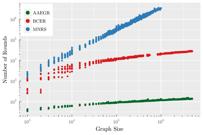
Figure 1: Comparison of the number of rounds until exact majority was found. Each dot is a individual test run.

We observe in Figure 1 that the absolute round count for our algorithm is quite high in comparison with the AAEGR protocol of [2]. Figure 2 suggests that both algorithms complete the computation within $\Theta(\log^{2}n)$ expected number of rounds, but our algorithm has a considerably higher constant factor in this bound. It seems that this high constant factor is the price we pay for provably guaranteeing the $O(\log^{2}n)$ bound in expectation and with high probability.

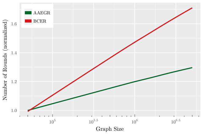
Figure 2: Comparison of the normalized number of rounds until exact majority was found. We computed for each data point the square root and calculated the average for each $n$

Leader Election

We compare our leader election algorithm with to the protocols proposed in [3] (protocol AG) and in [2] (protocol AAEGR). Algorithm [3] uses a state space of $\Theta\left(\log^{3}n\right)$ and each node starts with value 1. In each round, two nodes compete and compare their values. The winner increases its value and the looser changes to a minion state and decreases its value.

The algorithm of [2] uses $O\left(\log^{2}n\right)$ states. Each node can be in one of four modes. All nodes starts with the same state in a ’seeding mode’ where they utilize a syntetic coin flip to generate randomness. In the subsequent ’lottery mode,’ nodes try to increase their state values. During the tournament mode, nodes compare their values. The winner stays in competion, the looser changes to the minion mode and helps the leader candidate to win the competion faster by propagating its value to the other nodes.

Our algorithm contains several constants, which were optimized empirically. Each node is in one of 8 phases (states $q_{0}$ to $q_{7}$) and the constants have to be set so that no two nodes are in phases which are too far apart. For example, if a node is in state $q_{0}$ and another one is in state $q_{2}$, then they are too far apart. Starting with high constants (e.g. 100), we were gradually decreasing them for each phase seperatly until we found the smallest constant for each phase, where the property above is still valid. The results are shown in Table 1.

Phase	Constant
$q_{0}$	2
$q_{1}$	4
$q_{2}$	8
$q_{4}$	8
$q_{5}$	20
$q_{6}$	48, for $2^{\text{nd}}$ index
$q_{6}$	4, for $3^{\text{rd}}$ index
$q_{7}$	2, for spreading the message
$q_{7}$	33, for keeping the message

Table 1: Constants used for the simulations.

First, we compared the number of rounds for these three algorithms (see Figure 3). Again, the x-axis is the graph size and the y-axis is the average number of (parallel) rounds. We show two plots for our algorithm. The plot BCER is the running time of our algorithm, where the time is counted until a single $q_{9}$-node appears. We also plotted “BCER w.h.p.” where we stopped the algorithm as soon as one single $q_{6}^{0,0,0}$-node appeared and all other nodes were in the state $q_{3}$. This configuration leads to a single leader with high probability according to our theoretical analysis, and has always led to a single leader in our simulations.

The algorithm AAEGR of [2], with expected parallel time $O\left(\log^{5.3}n\right)$ shows a twofold behavior. In the first fast case, only one node has at the end the highest $phase$-$level$ combination. In this case, the process converges quickly, since the minions spread this information efficiently through the graph. In the second slow case, there are at least two nodes with the highest $phase$ value and none of them increased its level during the tournament mode. In this case, these two nodes have to meet in order to let one of them win the tournament. During our tests, roughly one third of all runs was in the slow case.

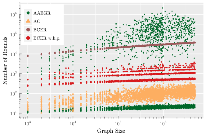
Figure 3: Comparison of the number of rounds until a leader was found. Each dot is a individual test run.

In Figure 4, we show the normalized number of rounds for each algorithm. The method to normalize these is the same as in exact majority case.

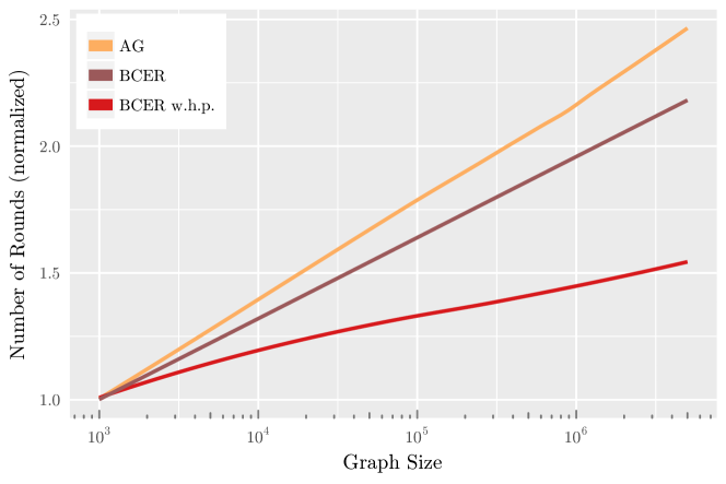
Figure 4: Comparison of the normalized number of rounds until a leader was found. We computed for each data point the square root and calculated the average for each $n$

References

- [1] D. Aldous and J. A. Fill. Reversible Markov Chains and random walks on graphs, 2002. Unfinished monograph, recompiled 2014, available at http://www.stat.berkeley.edu/$∼$aldous/RWG/book.html.
- [2] D. Alistarh, J. Aspnes, D. Eisenstat, R. Gelashvili, and R. L. Rivest. Time-space trade-offs in population protocols. In P. N. Klein, editor, Proceedings of the Twenty-Eighth Annual ACM-SIAM Symposium on Discrete Algorithms, SODA 2017, Barcelona, Spain, Hotel Porta Fira, January 16-19, pages 2560–2579. SIAM, 2017.
- [3] D. Alistarh and R. Gelashvili. Polylogarithmic-time leader election in population protocols. In M. M. Halldórsson, K. Iwama, N. Kobayashi, and B. Speckmann, editors, Automata, Languages, and Programming - 42nd International Colloquium, ICALP 2015, Kyoto, Japan, July 6-10, 2015, Proceedings, Part II, volume 9135 of Lecture Notes in Computer Science, pages 479–491. Springer, 2015.
- [4] D. Alistarh, R. Gelashvili, and M. Vojnovic. Fast and exact majority in population protocols. In C. Georgiou and P. G. Spirakis, editors, Proceedings of the 2015 ACM Symposium on Principles of Distributed Computing, PODC 2015, Donostia-San Sebastián, Spain, July 21 - 23, 2015, pages 47–56. ACM, 2015.
- [5] D. Angluin, J. Aspnes, Z. Diamadi, M. J. Fischer, and R. Peralta. Computation in networks of passively mobile finite-state sensors. Distributed Computing, 18(4):235–253, 2006.
- [6] D. Angluin, J. Aspnes, and D. Eisenstat. Fast computation by population protocols with a leader. Distributed Computing, 21(3):183–199, Sept. 2008.
- [7] A. Auger and B. Doerr. Theory of Randomized Search Heuristics: Foundations and Recent Developements. World Scientific, 2011.
- [8] F. Bénézit, P. Thiran, and M. Vetterli. Interval consensus: From quantized gossip to voting. In Proceedings of the IEEE International Conference on Acoustics, Speech, and Signal Processing, ICASSP 2009, 19-24 April 2009, Taipei, Taiwan, pages 3661–3664. IEEE, 2009.
- [9] P. Berenbrink, T. Friedetzky, P. Kling, F. Mallmann-Trenn, and C. Wastell. Plurality consensus via shuffling: Lessons learned from load balancing. CoRR, abs/1602.01342, 2016.
- [10] C. Cooper, R. Elsässer, H. Ono, and T. Radzik. Coalescing random walks and voting on connected graphs. SIAM J. Discrete Math., 27(4):1748–1758, 2013.
- [11] C. Cooper, R. Elsässer, T. Radzik, N. Rivera, and T. Shiraga. Fast consensus for voting on general expander graphs. In Distributed Computing - 29th International Symposium, DISC 2015, Tokyo, Japan, October 7-9, 2015, Proceedings, pages 248–262, 2015.
- [12] D. Doty and D. Soloveichik. Stable leader election in population protocols requires linear time. In Distributed Computing - 29th International Symposium, DISC 2015, Tokyo, Japan, October 7-9, 2015, Proceedings, 2015.
- [13] M. Draief and M. Vojnovic. Convergence speed of binary interval consensus. In INFOCOM 2010. 29th IEEE International Conference on Computer Communications, Joint Conference of the IEEE Computer and Communications Societies, 15-19 March 2010, San Diego, CA, USA, pages 1792–1800. IEEE, 2010.
- [14] R. M. Karp, C. Schindelhauer, S. Shenker, and B. Vöcking. Randomized rumor spreading. In 41st Annual Symposium on Foundations of Computer Science, FOCS 2000, 12-14 November 2000, Redondo Beach, California, USA, pages 565–574. IEEE Computer Society, 2000.
- [15] G. B. Mertzios, S. E. Nikoletseas, C. L. Raptopoulos, and P. G. Spirakis. Determining majority in networks with local interactions and very small local memory. In J. Esparza, P. Fraigniaud, T. Husfeldt, and E. Koutsoupias, editors, Automata, Languages, and Programming, volume 8572 of Lecture Notes in Computer Science, pages 871–882. Springer Berlin Heidelberg, 2014.
- [16] M. Raab and A. Steger. ”balls into bins” - A simple and tight analysis. In M. Luby, J. D. P. Rolim, and M. J. Serna, editors, Randomization and Approximation Techniques in Computer Science, Second International Workshop, RANDOM’98, Barcelona, Spain, October 8-10, 1998, Proceedings, volume 1518 of Lecture Notes in Computer Science, pages 159–170. Springer, 1998.
- [17] T. Sauerwald and H. Sun. Tight bounds for randomized load balancing on arbitrary network topologies. In 53rd Annual IEEE Symposium on Foundations of Computer Science, FOCS 2012, New Brunswick, NJ, USA, October 20-23, 2012, pages 341–350. IEEE Computer Society, 2012.