Stochastic modelling of non-stationary financial assets

Abstract

We model non-stationary volume-price distributions with a log-normal distribution and collect the time series of its two parameters. The time series of the two parameters are shown to be stationary and Markov-like and consequently can be modelled with Langevin equations, which are derived directly from their series of values. Having the evolution equations of the log-normal parameters, we reconstruct the statistics of the first moments of volume-price distributions which fit well the empirical data. Finally, the proposed framework is general enough to study other non-stationary stochastic variables in other research fields, namely biology, medicine and geology.

While several methodologies are available for modelling stationary processes, nature and complex processes in nowadays society is typically non-stationary. Examples range from the most fundamental turbulent fluids, weather dynamics and wind energy systems to human mobility, the brain signals and finance. In this paper we attack the problem of modelling non-stationary stochastic variables, addressing the specific example of financial volume-prices. We introduce a framework to model the evolution of non-stationary time series, applying it to the specific case of the volume-price of financial assets from 1750 companies at the New York Stock Exchange, collected from Yahoo database every 10 minutes during more than two years. Since the volume-price is typically a non-stationary stochastic variable but follows the same functional distribution, we assume that all time dependence of the variable is incorporated in time fluctuations of the distribution parameters, which are themselves stationary and evolve as coupled variables.

I Introduction

When addressing stochastic processes in nature, one of the fundamental assumptions is its stationary or non-stationary character. If the process is stationary, there is a probability density function associated to it, that does not change in time. In this case, the laws underlying series of measurements from the process can be assessed through proper averaging and computations of value series within finite size time-windows. However, the typical case found in nature is to observe processes whose probability density function changes also with time, making the derivation of the underlying laws more difficult.

In this paper we address a concrete example of a non-stationary stochastic process and show how to reproduce its statistical features, assuming not the strong condition of having time-invariant probability densities but only that all associated probability densities have a fixed functional form. In other words, having defined the function that best fits the probability density functions, its parameters are function of time. In particular, we will show that the parameters vary stochastically in time and follow a stationary process, which enables one to recover the non-stationary statistical moments characterizing the original process.

The framework here introduced is related to the so-called superstatistics approach introduce by Beck in the early nineties Beck (2008). Superstatistics is a branch of statistics aimed to the study of non-linear and non-equilibrium systems. Complex systems often show a behavior which can be regarded as a superposition of different dynamicsBeck (2008). We study the specific case of volume-price distributions in the New York Stock Exchange (NYSE), collected directly from Yahoo Finance. While the asset price shows how valuable the asset is and volume accounts for the corresponding market liquidity for that asset, the volume-price incorporates the interaction between both financial quantities, retrieving the total capitalization being transitioned in the market. Figure 1 shows the overview of the framework here proposed, with Fig. 1a illustrating the time-series of the price and volume of one single company.

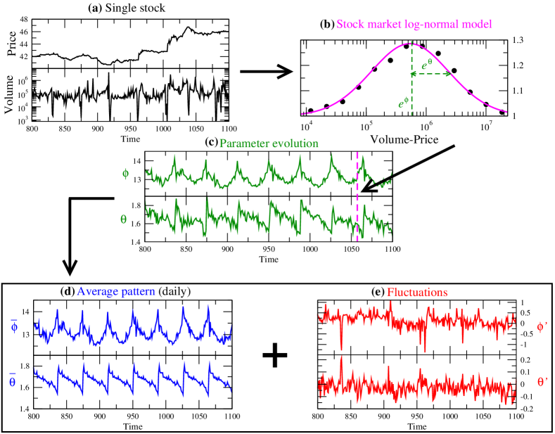
Figure 1: We start with the price and volume series of 1750 companies. In (a) we can see the volume and price series for just one of the companies. Multiplying the two series yields the volume-price series which follows a log-normal distribution with parameters $\phi$ and $\theta$. In (b) we can see the empirical density represented by the dots and the adjusted log-normal to the data, solid line, for a particular window of 10 minutes. Each 10-minutes window yields a log-normal with different parameters. Thus, we will have (c) a time series for the parameter $\phi$ and another one for $\theta$. Each time series can be decomposed in (d) a daily averaged pattern and (e) fluctuations around this pattern. We will describe the evolution observed in (c) by analyzing this components separately.

We start in Sec. II by assuming the log-normal distribution as the model for fitting each volume-price distribution from Yahoos’ database. Such assumptions is in line with previous findingsRocha et al. (2016). An example of the log-normal volume-price distribution is shown in Fig. 1b. The dots represent the empirical probability density function of the logarithm of the volume-price time series and the solid line is the theoretical log-normal distribution that best fits the data. Since the volume-price is non-stationary, the volume-price distribution varies in time, i.e. the two parameters defining the log-normal fit are time dependent, as illustrated in Fig. 1c. We then study the evolution of both parameters, considering that the two parameters include all the time dependency of the volume-price variable, and decompose the evolution of each parameter, into two separated additive contributions: an average behavior (Fig.  1d) and the corresponding stochastic fluctuations around it (Fig.  1e). While the average behavior is modelled with a polynomial in time for the time span of one day, the fluctuations are modelled through a system of two coupled stochastic differential equationsFriedrich et al. (2011). In particular, by knowing how the fluctuations of both parameters evolve in time, we will be able to retrieve the non-stationary evolution of the volume-price in the NYSE, namely the evolution of its statistical moments. Finally, in Sec.V we summarize the main conclusions and discuss possible applications of this work to other fields of study.

II Log-normal model for volume-prices

In the following we analyze the volume-price series of 1750 companies having listed shares in the New York Stock Exchange (NYSE), with a sampling frequency of $0.1$ min^-1. After removing all the after-hours trading and discarding all the days with recorded errors, our dataset contains 17708 data points for each company covering a total period of $976$ days. Figure 1a shows an illustrative example of the price and volume series of one specific company. All the data were collected from the website http://finance.yahoo.com/ and more details concerning its preprocessing may be found in the references of Rocha and co-workersRocha et al. (2015, 2014, 2016).

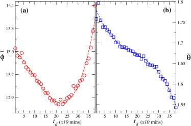
Figure 2: The average over all trading days of (a) parameter $\phi$ and (b) parameter $\theta$, with the corresponding fitting cubic polynomials (see text).

In previous works, it was shown that the log-normal distribution properly models the distribution of volume-price in each $10$-minute frameRocha et al. (2016). The probability density function (PDF) of the log-normal is:

$$p_{\phi,\theta}(s)=\frac{1}{s\sqrt{2\pi}\theta}\exp{\left[-\frac{(\log s-\phi)^{2}}{2\theta^{2}}\right]}$$ (1)

and is one of the common models in finance dataRocha et al. (2016); Camargo et al. (2013). Here $s$ symbolizes the volume-price. Parameter $\phi$ accounts for the mean and $\theta$ for the standard deviation of the logarithm volume-price series and they take different values for each $10$-minute frame. Consequently, fitting the volume-price distributions with Eq. (1) at each $10$-minute lag for the full $976$-day period yields two data series of values, one for $\phi$ and another for $\theta$.

II.1 Average behavior of the volume-price distribution

The original time series of $\phi$ and $\theta$ parameters is decomposed into the sum of their average daily patterns, $\overline{\phi}$ and $\overline{\theta}$, with the respective fluctuations, $\phi^{\prime}$ and $\theta^{\prime}$, around the average patterns:

$$\phi = \overline{\phi}+\phi^{\prime}\,,$$ (2a)

$$\theta = \overline{\theta}+\theta^{\prime}\,.$$ (2b)

In Figure 2 one sees the average patterns of $\phi$ and $\theta$, from which one can extract insight concerning the typical behavior of trades during the opening time, as follows. In Fig. 2a the average pattern of parameter $\phi$ is plotted. One notices that trading is heavier, i.e. larger values of $\phi$, at the beginning and end of the day compared to the rest of the day. Such feature reflects the fact that the opening and the closing of the NYSE are very peculiar times. In the beginning of the day, the volume-price series has high values, because it concentrates the information of the traders during the precedent closing period when traders postpone their next buy or sell to the next opening moment. After the opening one observes an approximately linear decrease of the trading activity, which in the second half of the day increases cubically. This higher rate in the end of the day may happen because traders react against a deadline, the closing time.

Close to the end of the day, volume-prices start to grow again, since traders try their last chance to buy and sell according to the market present state in a sort of herd behavior. This herd behavior can also be derived from the daily pattern of parameter $\theta$ plotted in Fig. 2b. In the beginning of the day there is a large variance in our data (large $\theta$), due to the different perceptions the traders have following a closing period where decisions were taken following different strategies and based in different alternative sources of information (e.g. open exchange markets elsewhere in the world). After that it decreases monotonically reflecting the tendency of traders to behave in the same way (small volume-price variance), since they based their decisions in the same real time prices of the NYSE, attaining a minimum at the closing time. Furthermore, during the day the standard deviation relaxes, showing a more constant value around noon. This value of $\theta$ in the middle of a (typical) day, being less sensitive to the opening and closing moments, defined through an inflexion point, should be characteristic of the specific stock exchange we are analyzing.

Both average patterns are well approximated, in mean-square sense, by cubic polynomials of time:

$$\bar{\phi}(t_{d}) = a_{\phi}t_{d}^{3}+b_{\phi}t_{d}^{2}+c_{\phi}t_{d}+d_{\phi}\,,$$ (3a)

$$\bar{\theta}(t_{d}) = a_{\theta}t_{d}^{3}+b_{\theta}t_{d}^{2}+c_{\theta}t_{d}+d_{\theta}\,,$$ (3b)

where $t_{d}=(t\pmod{144})-54$ in units of $u=10$ minutes, and $a_{\phi}=8.2\times 10^{-5}$, $b_{\phi}=-2.3\times 10^{-3}$, $c_{\phi}=-2.0\times 10^{-2}$, $d_{\phi}=13.52$, $a_{\theta}=-1.0\times 10^{-5}$, $b_{\theta}=5.6\times 10^{-4}$, $c_{\theta}=-1.3\times 10^{-2}$ and $d_{\theta}=1.79$.

Note that the market is only open for normal trading during $6$h$30$min ($39\times 10$min). Outside of the normal trading period we consider $\bar{\phi}$ and $\bar{\theta}$ to be zero. These cubic models for the average daily pattern, depend on the data set being analyzed, i.e. on the stock market, and typical maxima and minima values of both parameters, as well as their inflexion points can be straightforwardly estimated.

II.2 Modelling stochastic fluctuations of the parameters

The fluctuations around the patterns in Fig. 2 were obtained by subtracting the 20-day moving average pattern (Fig. 1d) from the corresponding parameter (Fig. 1c), yielding the fluctuations $\phi^{\prime}$ and $\theta^{\prime}$ illustrated in Fig. 1e.

Important for the modelling of the fluctuations is to separate them from all periodic modes of the time variation of each parameter. Figures 3a and 3b show the power spectrum of the original parameters (black lines) and the corresponding fluctuations (colored points). As one clearly sees, the periodic peaks, observed for the original parameter, are not present in the spectra of their fluctuations, showing that the periodic behavior is properly detrended.

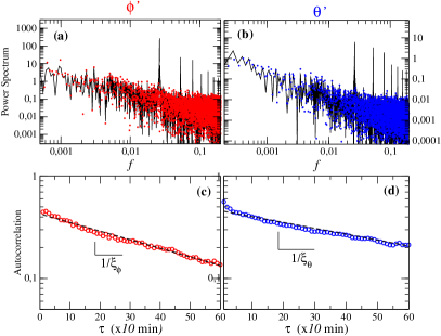
Figure 3: (a) Power spectrum of the $\phi$ time series and (b) of the $\theta$ series, both detrended (see text). (c) Autocorrelation function (circles) and linear function fitted to the data (dashed lines) in a log-lin scale for the $\phi$ time series and (d) for the $\theta$ time series.

In Figs. 3c and 3d we plot the autocorrelation function $\alpha$ for the fluctuations $\phi^{\prime}$ and $\theta^{\prime}$ respectively, showing a clear exponential decay which is modelled as

$$\alpha_{\phi^{\prime},(\theta^{\prime})}=\beta_{\phi^{\prime},(\theta^{\prime})}\exp{\left(-\frac{\tau}{\xi_{\phi^{\prime},(\theta^{\prime})}}\right)}.$$ (4)

For $\phi^{\prime}$ one obtains $\xi_{\phi^{\prime}}=52.08\times 10$ mins and $\log(\beta_{\phi^{\prime}})=-0.8496$, while for $\theta^{\prime}$ one obtains $\xi_{\theta^{\prime}}=75.76\times 10$ s and $\log(\beta_{\theta})=-0.7776$. In other words, one surprisingly finds that, while the logarithm average fluctuation $\phi^{\prime}$ looses memory beyond one daily cycle of the stock market (open during 9 hours) the fluctuation of lognormal variances shows a memory beyond the closing of the stock market, probably incorporating information from after-hour tradings.

Figure 4: Marginal probability density function (black) and Gaussian adjusted PDF (red) of the detrended (a) $\phi$ parameter and (b) $\theta$ parameter time series.

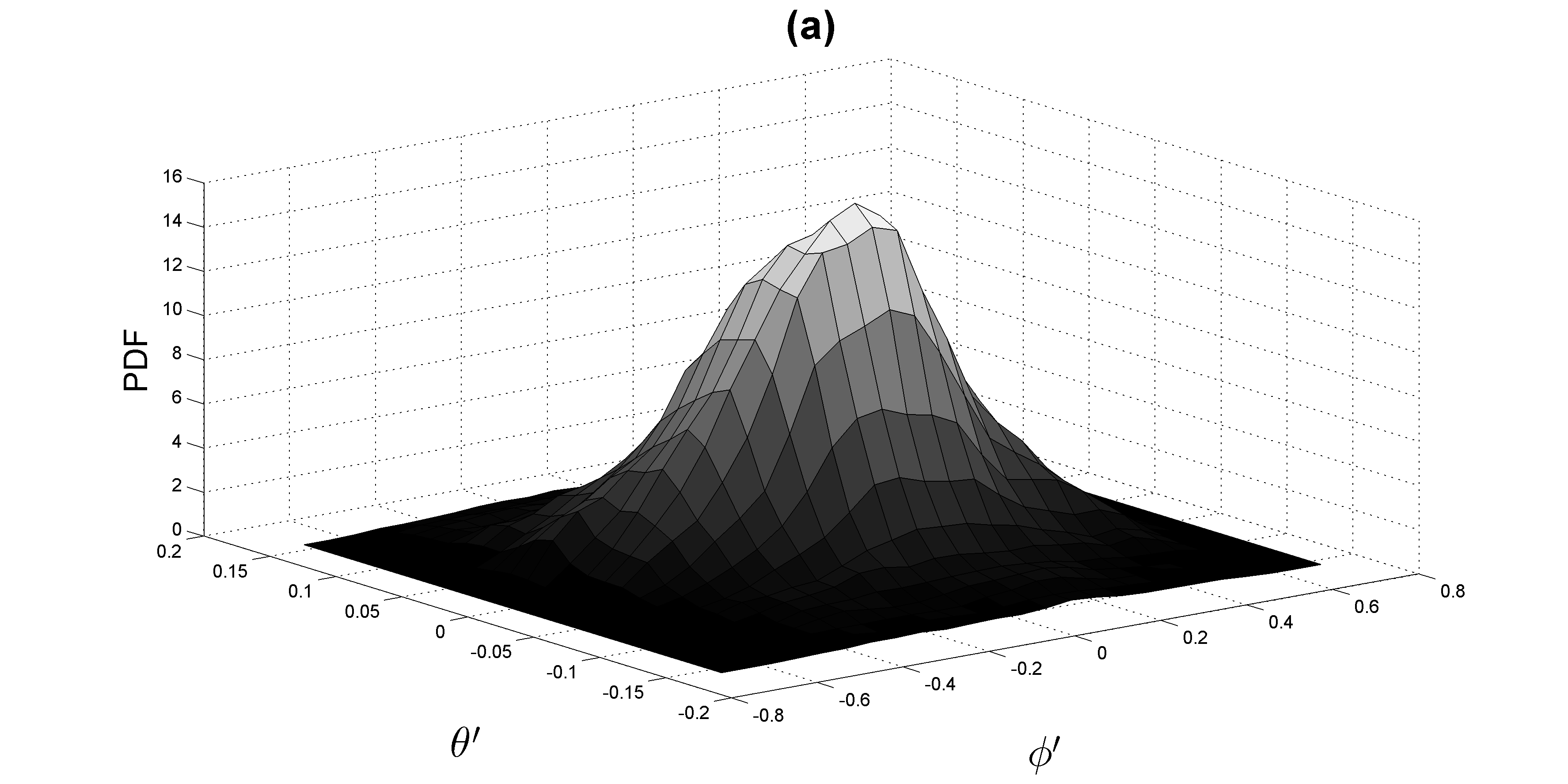
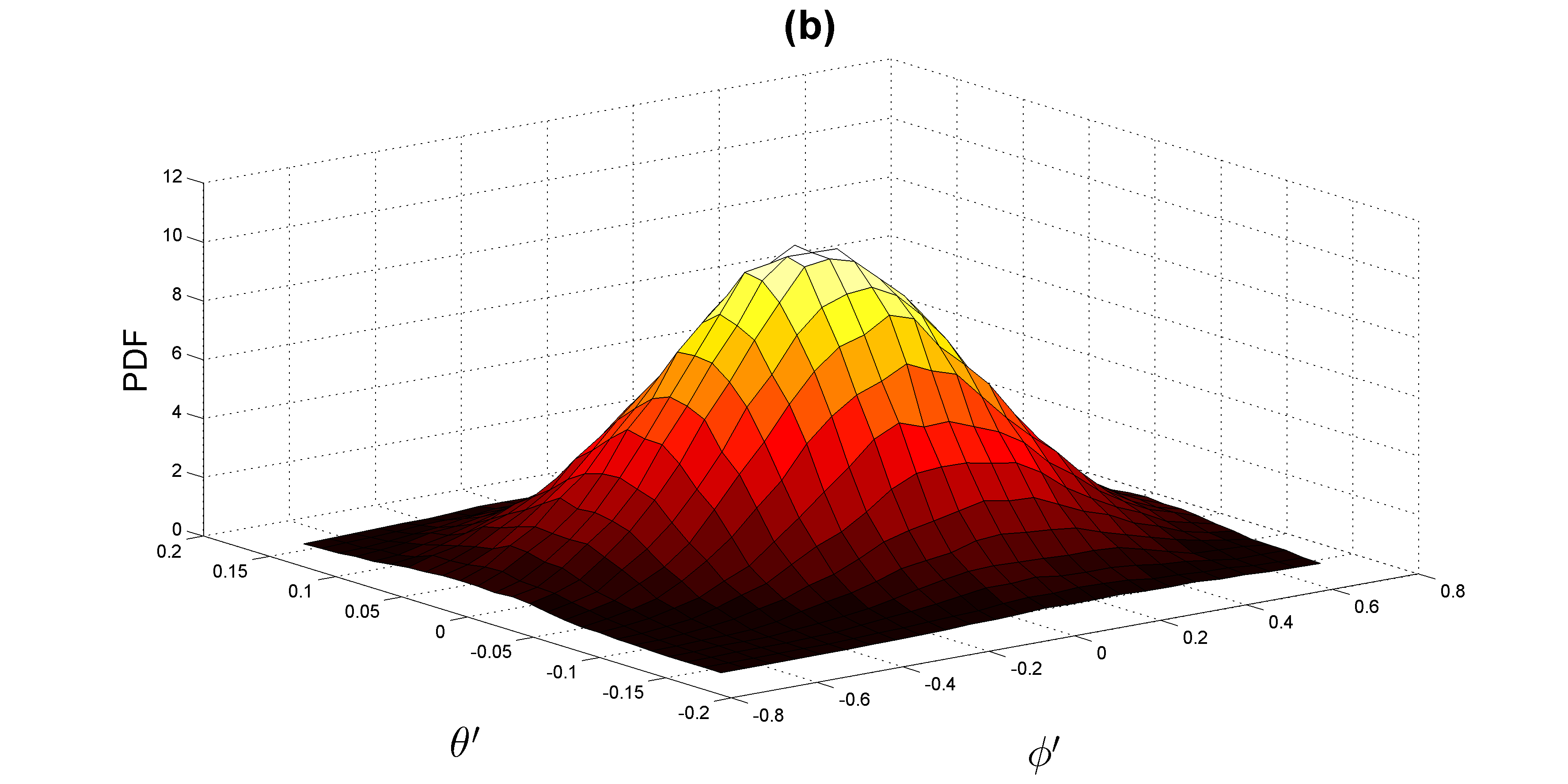
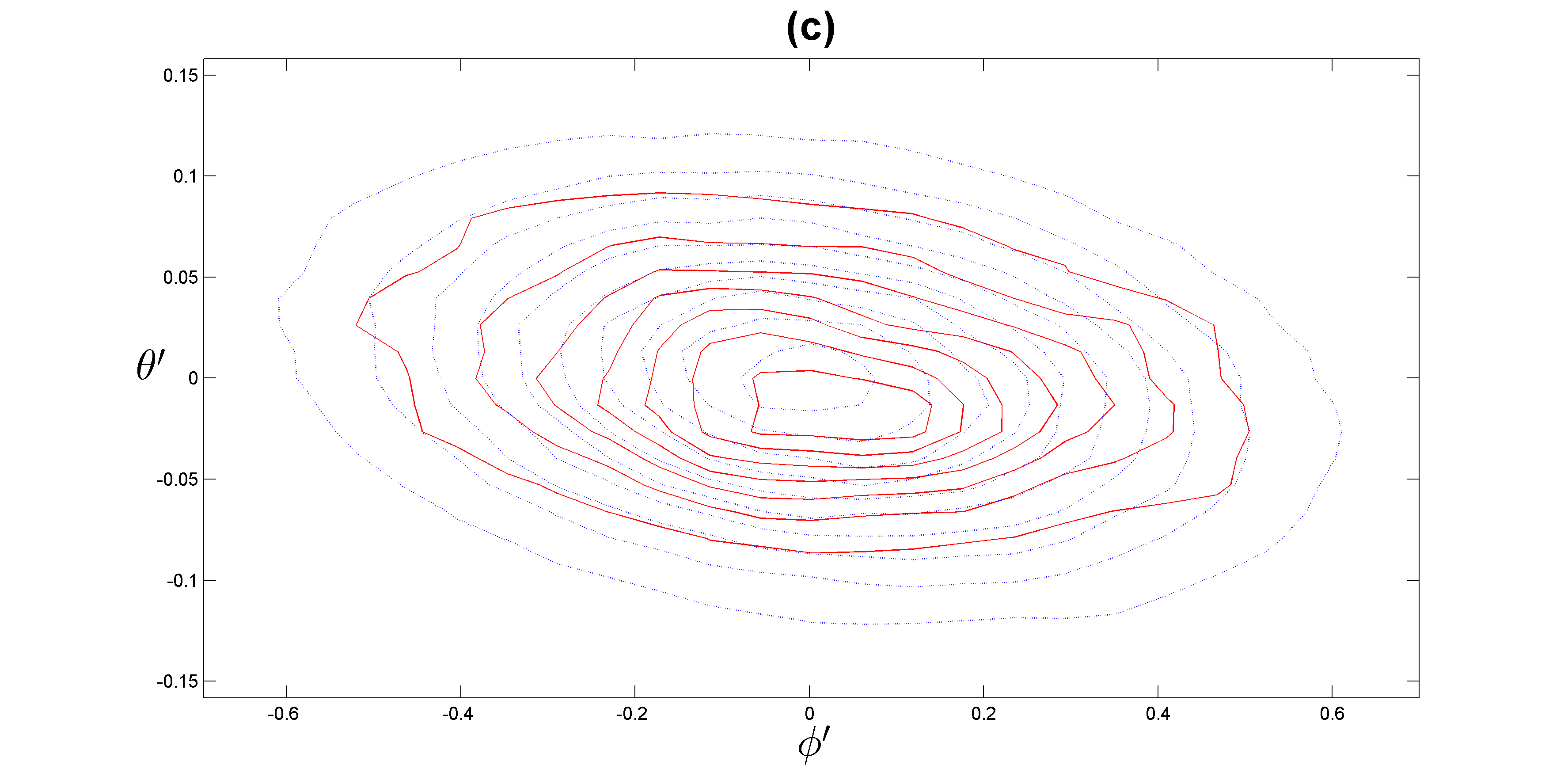
Figure 5: (a) Joint PDF of the empirical time series and (b) a multivariate normal distribution with mean vector and covariance matrix equal to the ones of our empirical data. (c) Contour plot of both empirical and theoretical joint PDFs in (a) and (b) respectively.

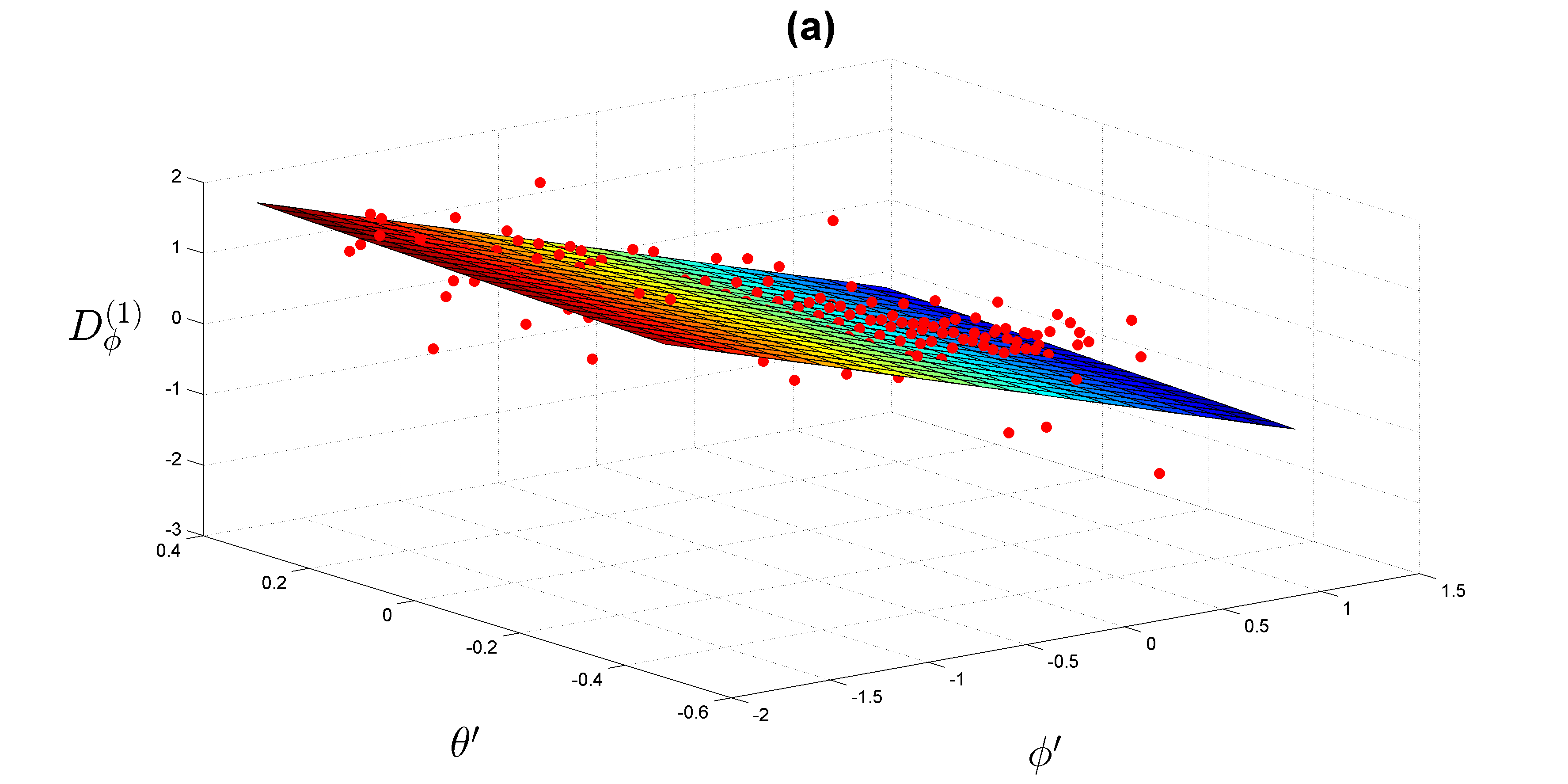
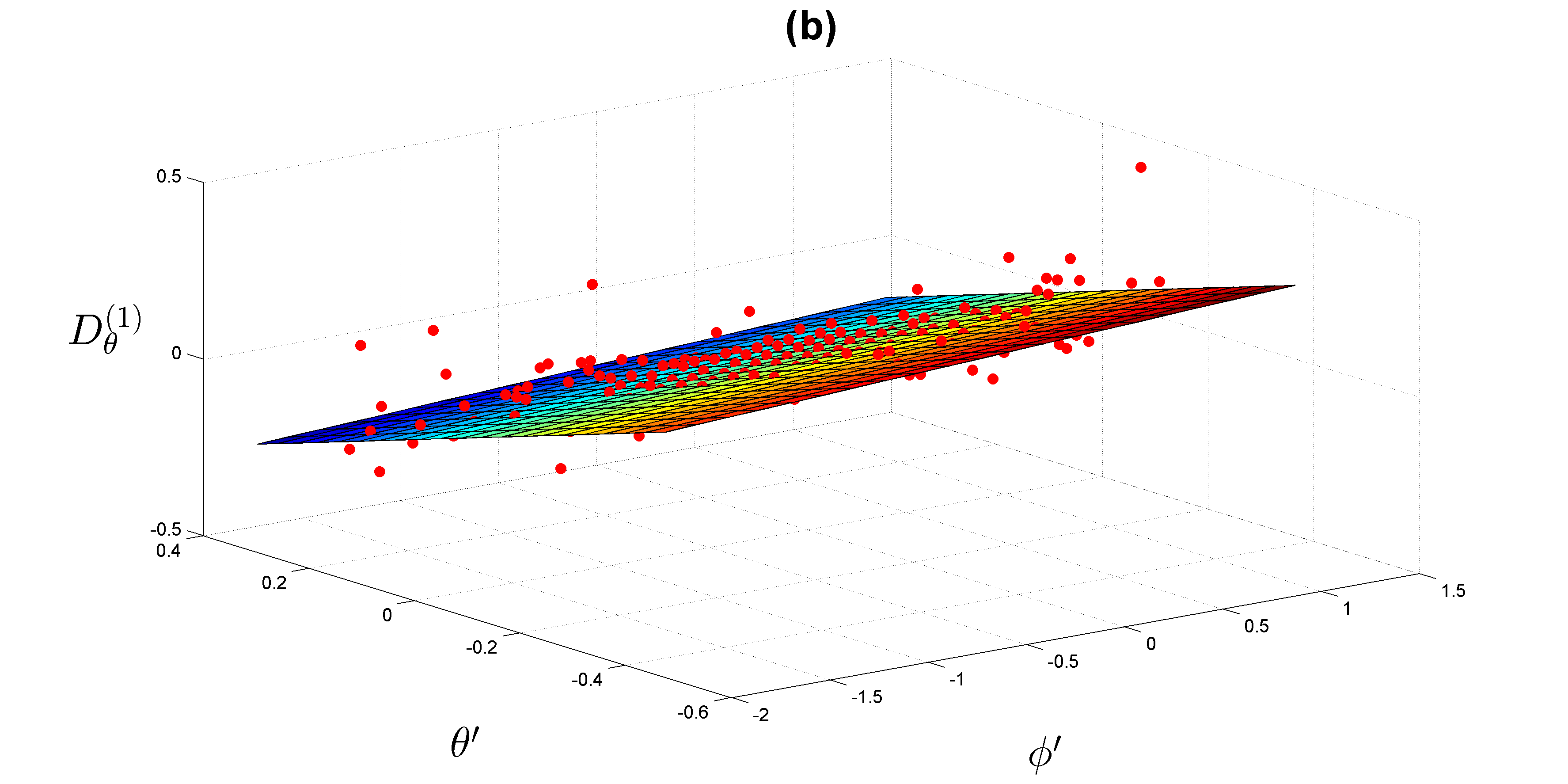
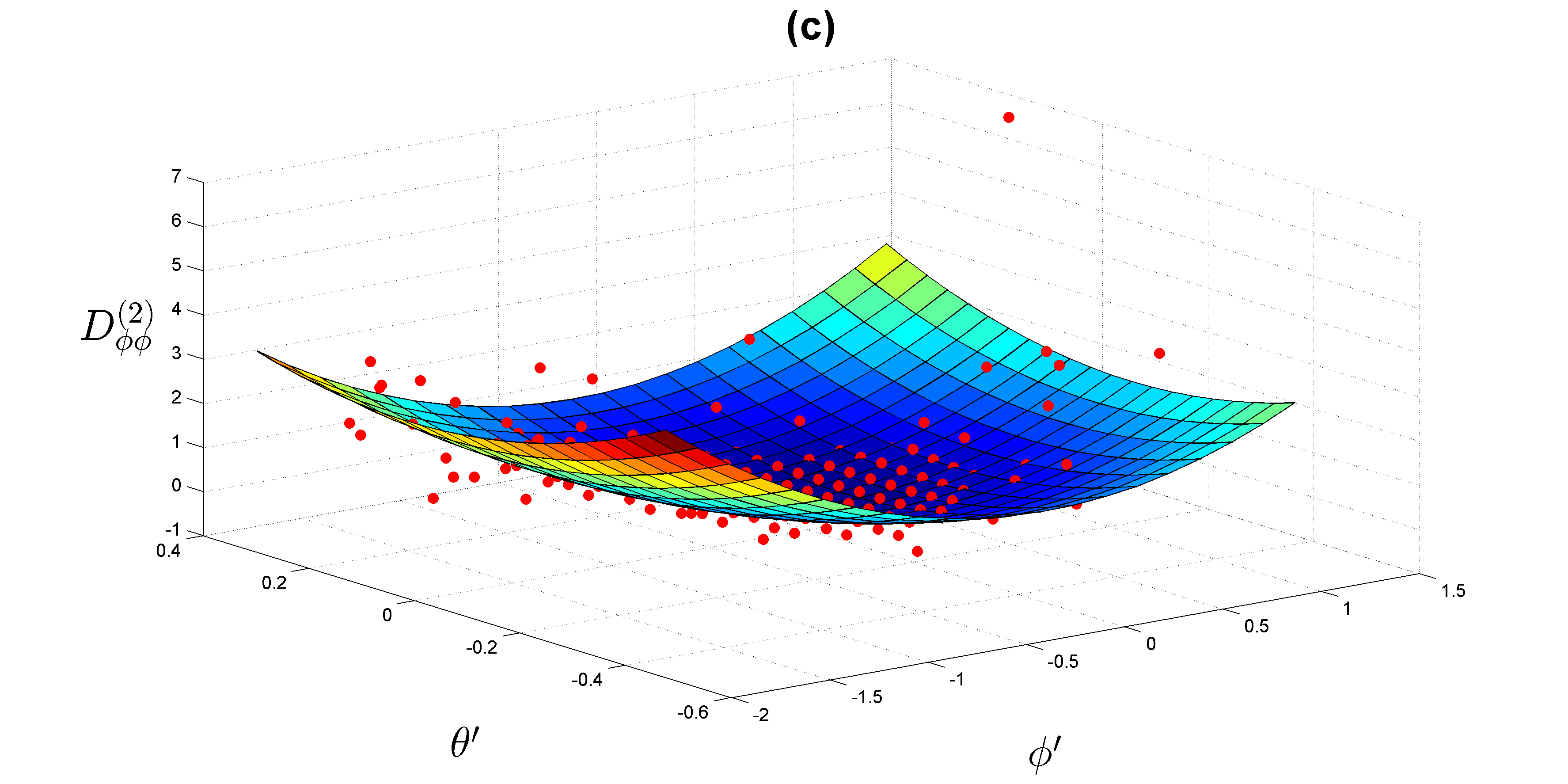
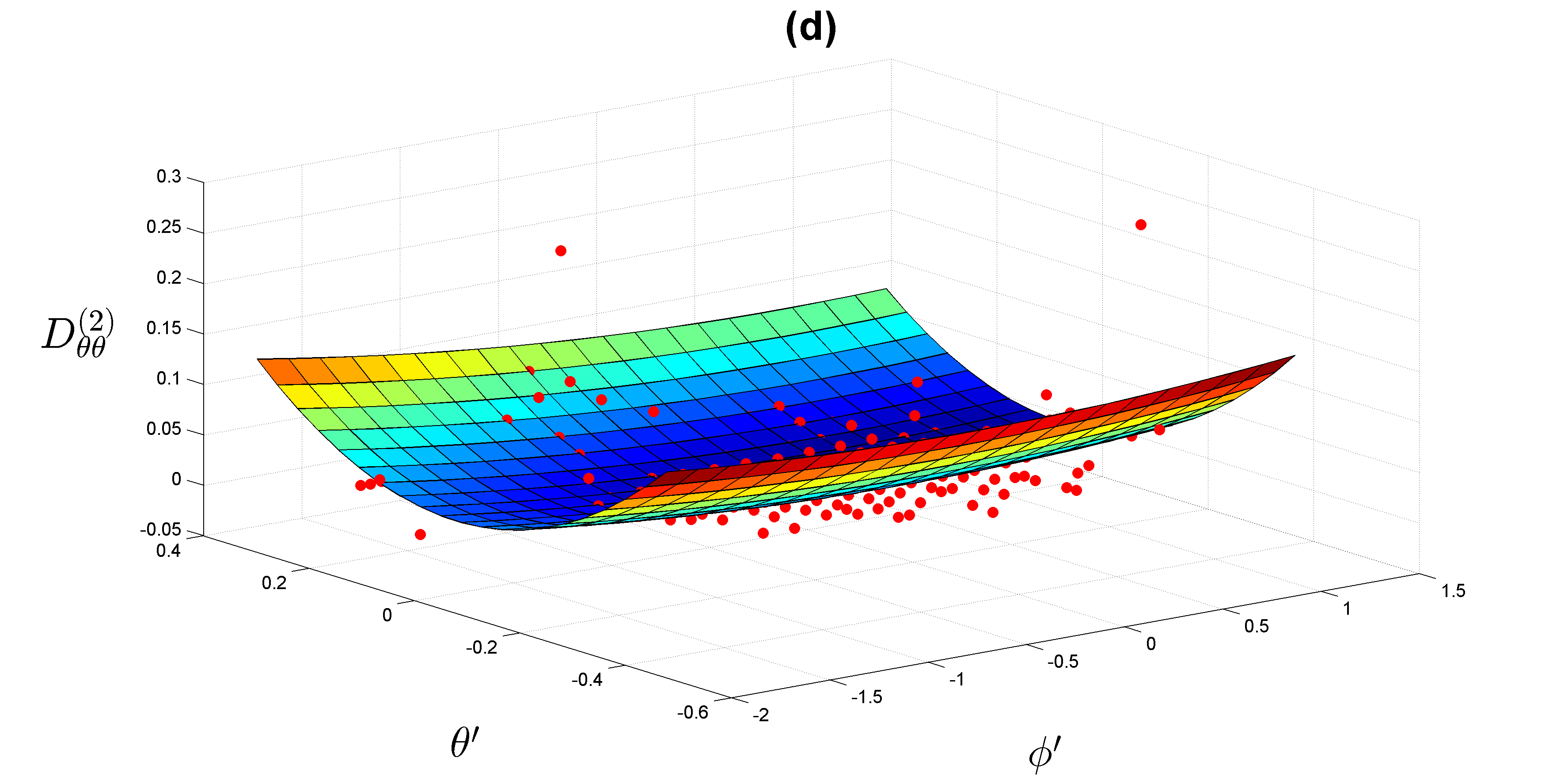
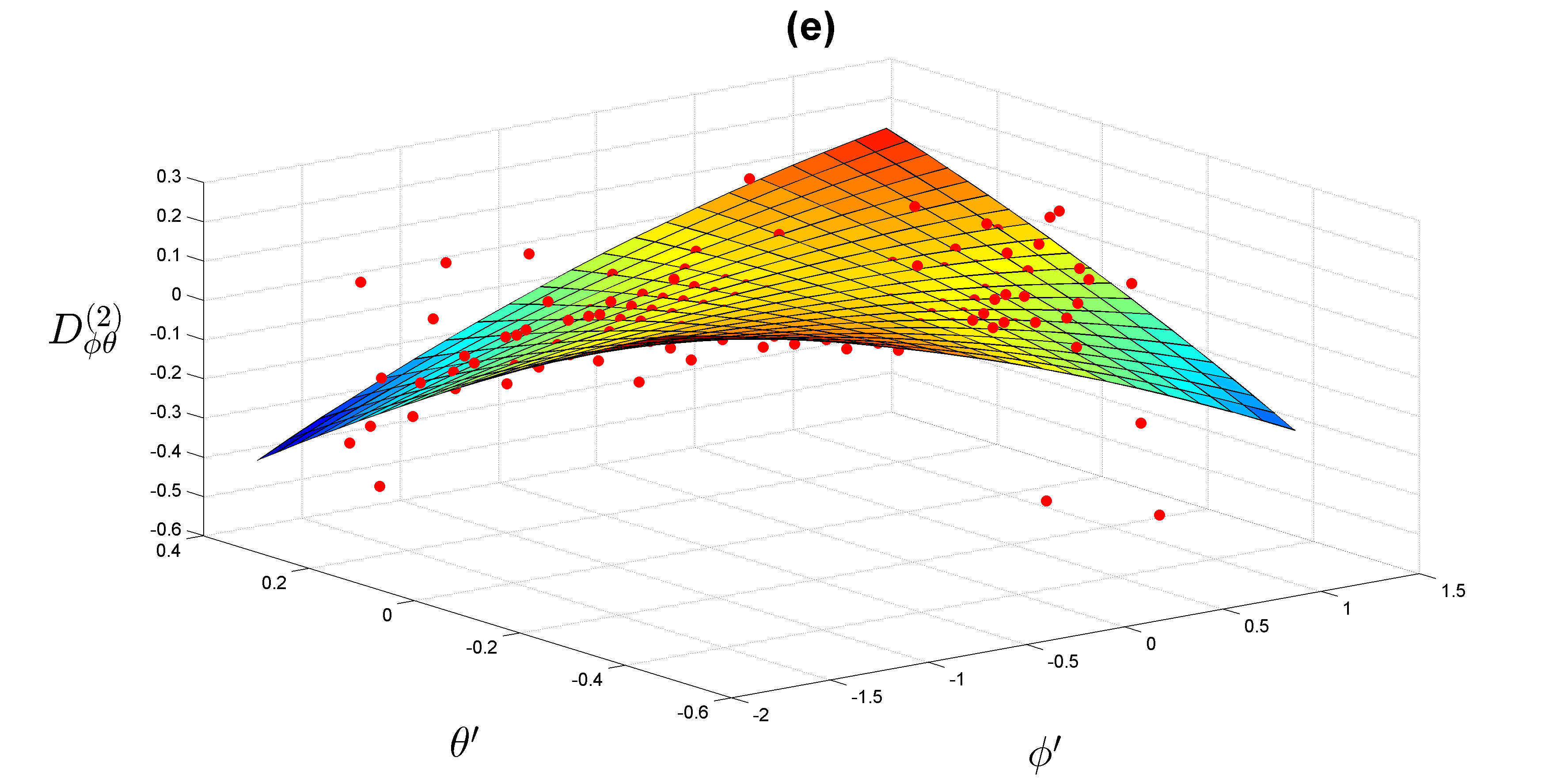
Figure 6: (a) Drift coefficient of the $\phi$ component, ${D_{\phi}}^{(1)}$, (b) Drift coefficient of the $\theta$ component, ${D_{\theta}}^{(1)}$. The three components of the diffusion matrix: (c) function $D^{(2)}_{\phi\phi}$, (d) function $D^{(2)}_{\theta\theta}$ and (e) function $D^{(2)}_{\phi\theta}$.

To end this section we show that both fluctuations, $\phi^{\prime}$ and $\theta^{\prime}$, are stochastic variables with a joint Gaussian distribution and anti-correlated with each other.

Figures 4a and 4b show the marginal PDF of the fluctuations $\phi^{\prime}$ and $\theta^{\prime}$ respectively (colored symbols) compared with the respective Gaussian, having the same mean and variance (dashed lines). The central region of the marginal PDF of $\theta^{\prime}$ is in good agreement with the Gaussian function, presenting deviations at the most outer regions. Apparently, for $\phi^{\prime}$ the Gaussian approximation is not as good as for $\theta^{\prime}$. However, the deviations from the Gaussian functional shape of the marginal distribution of $\theta^{\prime}$ is due to the fact that both parameter fluctuations are correlated as can be seen in Fig. 5.

Indeed, computing the covariance matrix

$$\mathbf{\Sigma}=\left[\begin{array}[]{cc}\Sigma_{\phi^{\prime}\phi^{\prime}}&\Sigma_{\phi^{\prime}\theta^{\prime}}\cr\Sigma_{\theta^{\prime}\phi^{\prime}}&\Sigma_{\theta^{\prime}\theta^{\prime}}\end{array}\right]=\left[\begin{array}[]{cc}0.0619&-0.0036\cr-0.0036&0.0039\end{array}\right].$$

Being a non-diagonal matrix, the covariance matrix shows that both parameter fluctuations are correlated. Consequently, the joint distribution $\rho(\phi^{\prime},\theta^{\prime})$ of both correlated parameters can be well fitted with a two-dimensional Gaussian distribution of correlated variables asForbes et al. (2011):

$$\rho(\phi^{\prime},\theta^{\prime})=\frac{1}{2\pi\sqrt{|\mathbf{\Sigma}|}}\exp{\left(-\frac{1}{2}(\mathbf{x}-\mathbf{\mu})^{T}\mathbf{\Sigma}^{-1}(\mathbf{x}-\mathbf{\mu})\right)},$$ (5)

where $\mathbf{x}=(\phi^{\prime},\theta^{\prime})$, $|\mathbf{\Sigma}|=\Sigma_{\phi^{\prime}\phi^{\prime}}\Sigma_{\theta^{\prime}\theta^{\prime}}-\Sigma_{\phi^{\prime}\theta^{\prime}}^{2}$ is the determinant of the covariance matrix $\mathbf{\Sigma}$ and $\mathbf{\mu}=(\mu_{\phi^{\prime}},\mu_{\theta^{\prime}})$ is the two-dimensional vector of the means of both parameter fluctuations. Since we are addressing the joint distribution of fluctuations of both parameters around their average pattern $\mathbf{\mu}\sim 0$. In Fig. 5a one sees the joint histogram of both parameter fluctuations, while in Fig. 5b the joint density function in Eq. (5) with the same covariance matrix $\mathbf{\Sigma}$ and means $\mathbf{\mu}$ is shown. From the respective contour plots in Figs. 5c and 5d one identifies a reasonable match. Moreover, one notices that both contour plots lean towards the left, indicating a negative correlation, i.e. $\Sigma_{\phi^{\prime}\theta^{\prime}}<0$.

Being correlated, the parameter fluctuations must be modelled as a pair of coupled variables. The model for the pair of parameter fluctuations is described in the next section.

III The stochastic evolution of log-normal parameters

For modelling the two fluctuations, $\phi^{\prime}$ and $\theta^{\prime}$, we consider them as stochastic variables that evolve coupled to each other according to a two-dimensional Markov process with two independent stochastic Gaussian white noise sources. The conditions that enable us to settle down such assumptions will be addressed in the end. Even in the case that the conditions do not hold rigorously, it is possible to apply this framework, as discussed previously in Ref. Rocha et al. (2016) and below. For simplicity, in this section we are going to suppress the prime symbol noticing that we only address the fluctuations.

Our model is given by a system of two coupled Langevin equations, namely

$$\begin{bmatrix}d\phi(t)\\ d\theta(t)\end{bmatrix} = \begin{bmatrix}{D_{\phi}}^{(1)}(\phi,\theta)\\ {D_{\theta}}^{(1)}(\phi,\theta)\end{bmatrix}dt$$ (6)

$$+ \begin{bmatrix}g_{\phi\phi}(\phi,\theta)&g_{\phi\theta}(\phi,\theta)\\ g_{\theta\phi}(\phi,\theta)&g_{\theta\theta}(\phi,\theta)\end{bmatrix}\begin{bmatrix}dW^{(1)}_{t}\\ dW^{(2)}_{t}\end{bmatrix}$$ (8)

where for either $X=\phi$ or $X=\theta$

$$D_{X}^{(1)}(\phi^{\ast},\theta^{\ast})=\lim_{\tau\rightarrow 0}\frac{1}{k!\tau}\left\langle\left(X(t+\tau)-X(t)\right)\right\rangle_{X(t)=\phi^{\ast},Y(t)=\theta^{\ast}}$$ (9)

with $\langle\cdot\rangle$ meaning the average over all pairs $(X(t),Y(t))$ of the parameter pair $(\phi,\theta)$ respectively and where $\mathbf{g}\mathbf{g}^{T}=\mathbf{D}^{(2)}$ with

$$\mathbf{D}^{(2)}=\begin{bmatrix}D^{(2)}_{\phi\phi}&D^{(2)}_{\phi\theta},\\ D^{(2)}_{\theta\phi}&D^{(2)}_{\theta\theta},\\ \end{bmatrix}$$ (10)

such that, for the component $[XY]$ in matrix $\mathbf{D}^{(2)}$, one has

$$D_{XY}^{(2)}(\phi^{\ast},\theta^{\ast})=\lim_{\tau\rightarrow 0}\frac{1}{k!\tau}\left\langle\left(X(t+\tau)-X(t)\right)\left(Y(t+\tau)-Y(t)\right)\right\rangle_{X(t)=\phi^{\ast},Y(t)=\theta^{\ast}}\,.$$ (11)

Here $\phi^{\ast}$ and $\theta^{\ast}$ label one specific bin.

The two stochastic contributions, $dW^{(1)}_{t}$ and $dW^{(2)}_{t}$, are two independent Wiener processes, i.e.

$$\langle dW^{(n)}_{t}\rangle = 0,$$ (12a)

$$\langle dW^{(n)}_{t}dW^{(m)}_{t^{\prime}}\rangle = \delta_{mn}\delta(t-t^{\prime}),$$ (12b)

with $n,m=1,2$.

The drift vector $({D_{\phi}}^{(1)},{D_{\theta}}^{(1)})$ and the diffusion matrix $\mathbf{D}^{(2)}$ can be straightforwardly obtained from the sets of data using a recently package implemented in $R$ and available as open source at CRAN platformRinn et al. (2016).

	1	$\phi$	$\theta$	$\phi^{2}$	$\phi\theta$	$\theta^{2}$	$R^{2}$
$D^{(1)}_{\phi}$	-0.0085	-0.7143	0.2812	–	–	–	0.78
$D^{(1)}_{\theta}$	-0.0031	0.0293	-0.5023	–	–	–	0.67
$g_{\phi\phi}$	0.2185	0.0918	0.2255	0.4850	0.2925	4.0541	0.93
$g_{\theta\theta}$	0.0360	0.0174	-0.0128	0.0210	0.0245	1.5197	0.92
$g_{\phi\theta}$	-0.0111	-0.0051	-0.0158	-0.0134	0.2936	-0.1835	0.93

Table 1: Coefficients for the drift vector $\mathbf{D}^{(1)}$ and matrix $\mathbf{g}$, obtained by the Langevin analysis. For each fit one also gives the $R^{2}$ value of the corresponding least square fit.

In Fig. 6 we plot the drift vector and the diffusion matrix $\mathbf{D}^{(2)}$ obtained with this package. The empirical results (bullets) of all drift and diffusion functions are compared with their polynomial fit (surfaces), linear forms for the two drift coefficients and quadratic forms for the diffusion coefficients. The derivation of matrix $\mathbf{g}$ from the diffusion matrix is described in detail in Ref. Vasconcelos et al. (2011): since the diffusion matrix yields $\mathbf{D}^{(2)}=\mathbf{g}\mathbf{g}^{T}$ and has components fitted by quadratic forms of $\phi$ and $\theta$, matrix $\mathbf{g}$ can also have entries given by higher-order polynomials. Our results have shown that polynomials of degree one to the functions composing the drift vector and polynomials of degree two to the functions composing matrix $\mathbf{g}$ yield good results:

$$D^{(1)}(\phi,\theta) \approx a+b\phi+c\theta\,,$$ (13a)

$$g(\phi,\theta) \approx a+b\phi+c\theta+d\phi^{2}+e\phi\theta+f\theta^{2}\,.$$ (13b)

In Tab. 1 we show the values of all polynomial coefficients as well as the $R^{2}$ value of each fit.

The drift coefficients appear to depend linearly with respect to both parameter fluctuations: the fluctuations are subjected to a restoring force proportional to their amplitude. The restoring force for $\phi$ (logarithmic mean) fluctuations is stronger than the one for $\theta$ (logarithmic variance) fluctuations, indicating a faster relaxation of the dynamics towards the equilibrium value of the logarithmic mean, $\phi_{0}$, compared to the relaxation of the logarithmic variance, which can be associated to a measure of volume-price volatility.

In what concerns the diffusion matrix, one can detect a dominance of the quadratic term in $\theta$ for both diagonal terms in matrix $\mathbf{g}$. It seems that the variance of both fluctuations is governed mainly by the value of the logarithm variance itself. This makes sense since the variance of the fluctuations is responsible for the variance of the volume-price.

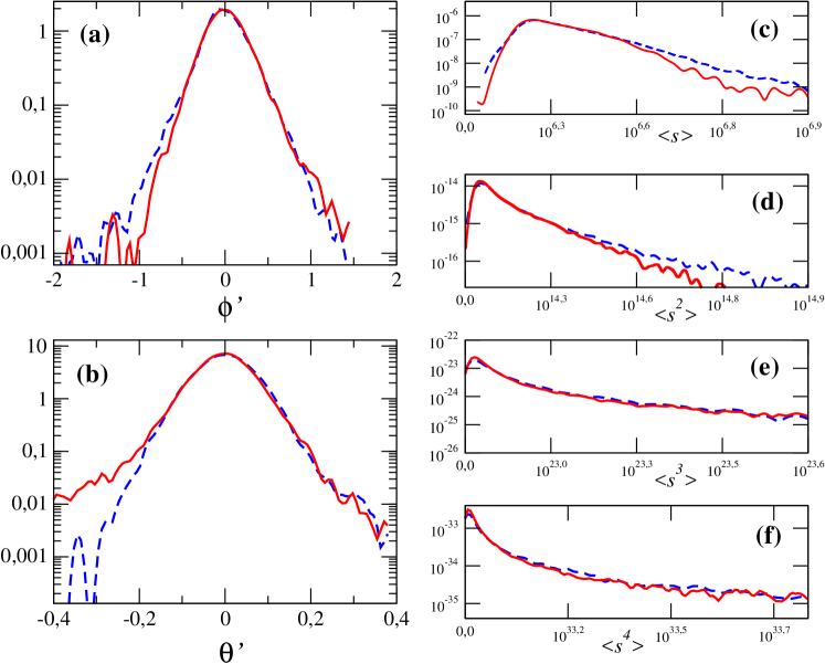
Figure 7: (a) Comparison between the PDFs of the empirical fluctuations of $\phi$ (dashed line) and the modelled increments (solid line) in a lin-log scale. (b) Same comparison is shown for $\theta$. (c-f) PDFs of the time series of the $n$-order moments $\langle s^{n}\rangle$ for $n=1,2,3,4$. The dashed line represents the empirical PDF and the solid line is the PDF obtained from our model. Each series is composed by $16918$ points.

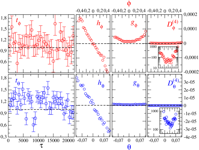
Figure 8: On the left, results of the Wilcoxon test to the detrended time series, $\phi$ and $\theta$, showing the $t$-values. Here, both series are considered separately. In the middle, the drift $h$ and diffusion $g$, for both series. On the right, the fourth Kramers-Moyal coefficient $D^{(4)}$ is plotted and in the inset the large values of $D^{(4)}/(D^{(2)})^{2}$ plotted show that conditions for Pawula theorem are not exactly met (see text).

IV Approaching non-stationarity

In the two previous sections we introduce our framework to extract a model for the quantities $\phi$ and $\theta$ parameterizing the log-normal distribution fitting the volume-prices at each 10-minute frame. As mentioned above, we have assumed that all time dependency is incorporated in the two parameters and that they are decomposable into an average pattern and fluctuations. In this section we show that, with such a framework, one is able to fully characterize the non-stationary time series of the volume-price.

To that end, we first deduce the formula of all moments of the log-normal distribution in Eq. (1), for all integer $n$, namely

$$\langle s^{n}\rangle=\int_{-\infty}^{+\infty}s^{n}p_{\phi,\theta}(s)ds=e^{n\phi+\frac{n^{2}\theta^{2}}{2}}\equiv F_{n}(\phi,\theta)\ .$$ (14)

It is a well known statistical resulsForbes et al. (2011) that, if one has all the moments of a distribution, one can deduce its probability density function using a Fourier transform. Therefore, we need to derive from our models for the average parameter patterns and parameter fluctuations the evolution equation of all moments as recently suggested in Ref. Rocha et al. (2016).

Next, we will do this explicitly, by assuming that, similarly to $\phi$ and $\theta$, all moments are also separated in an average pattern and fluctuations around it.

The “average” $n$-order moments of the volume-price, $\langle\overline{s}^{n}\rangle$, is given by the expression in Eq. (14), substituting $\phi$ and $\theta$ by $\overline{\phi}$ and $\overline{\theta}$ respectively.

The fluctuations of the volume-price moments follow also the expression in Eq. (14) with the parameter fluctuations following the system of Langevin equations given in Eq. (6) and can be derived through the Itô expansionVasconcelos et al. (2011) when differentiating the expression in Eq. (14) with respect to time, yieldingRocha et al. (2016)

$$d\langle s^{n}\rangle = A_{n}(\phi(t),\theta(t))dt+B_{n}(\phi(t),\theta(t))dW_{1}$$ (17)

$$+C_{n}(\phi(t),\theta(t))dW_{2}$$

with

$$A_{n}(\phi(t),\theta(t)) = \frac{\partial F_{n}}{\partial\phi}h_{1}+\frac{\partial F_{n}}{\partial\theta}h_{2}$$ (18a)

$$+ \frac{\partial^{2}F_{n}}{\partial\phi\partial\theta}(g_{11}g_{21}+g_{12}g_{22})$$ (18c)

$$+ \frac{1}{2}\frac{\partial^{2}F_{n}}{\partial\phi^{2}}(g^{2}_{11}+g^{2}_{12})$$ (18e)

$$+ \frac{1}{2}\frac{\partial^{2}F_{n}}{\partial\theta^{2}}(g^{2}_{21}+g^{2}_{22})\,,$$ (18g)

$$B_{n}(\phi(t),\theta(t)) = \frac{\partial F_{n}}{\partial\phi}g_{11}+\frac{\partial F_{n}}{\partial\theta}g_{21}\,,$$ (18i)

$$C_{n}(\phi(t),\theta(t)) = \frac{\partial F_{n}}{\partial\phi}g_{12}+\frac{\partial F_{n}}{\partial\theta}g_{22}\,.$$ (18k)

$$\frac{\partial F_{n}}{\partial\phi} = nF_{n}(\phi,\theta)$$ (18m)

$$\frac{\partial F_{n}}{\partial\theta} = n^{2}\theta F_{n}(\phi,\theta)$$ (18o)

$$\frac{\partial^{2}F_{n}}{\partial\phi^{2}} = n^{2}F_{n}(\phi,\theta)$$ (18q)

$$\frac{\partial^{2}F_{n}}{\partial\theta^{2}} = n^{4}\theta^{2}F_{n}(\phi,\theta)$$ (18s)

$$\frac{\partial^{2}F_{n}}{\partial\phi\partial\theta} = n^{3}\theta F_{n}(\phi,\theta)$$ (18u)

Equation (17) is a non-homogeneous stochastic differential equation with “drift” and “diffusion” functions depending on time.

In Fig. 7a and 7b we compare the empirical distribution of the fluctuations $\phi^{\ast}$ and $\theta^{\ast}$ respectively, with the corresponding modelled distribution obtained by integrating Eq. (6). Within a range of fluctuations beyond one standard deviation the modelled distribution fits well the empirical distributions. The drift and diffusion functions were derived as described, adjusting them afterwards to optimize the $R^{2}$ of the distributions in Figs. 7(a-b) without deviating significantly from the least square fits of the surfaces in Fig. 6.

In Figs. 7(c-f) we plotted the empirical and theoretical probability distributions of $\langle s^{n}\rangle,n=1,...,4$, showing also good agreement. The empirical moments are obtained by replacing in Eq. ((14)) the original time series of $\phi$ and $\theta$. Our model has a good fit in the first moments and can be used to model them since the theoretical and empirical distributions are very close to each other. Since the $\phi$ parameter is better modelled than the $\theta$ parameter, it is expected that for higher moments, when $\theta$ is dominant over $\phi$ we do not achieve such good results.

In order to apply a Langevin model, it is necessary that the fluctuations time series, $\phi^{\prime}$ and $\theta^{\prime}$, are Markovian. To test the Markov property of the data series, we compute the transition probabilities $p(x_{1},\tau_{1}|x_{2},\tau_{2};x_{3},\tau_{3})$ and compare it with the two point conditional probabilities $p(x_{1},\tau_{1}|x_{2},\tau_{2})$. For that we use Wilcoxon rank-sum test Renner et al. (2001). Values of $t/t_{0}$ close to 1, indicates the data has the Markovian property, which, as shown in Fig. 8 (left), is observed already for the smallest values of time increments.

We also computed the $D_{4}$ function for both time fluctuations series, to test if the conditions to apply Pawula Theorem are fulfilledRisken (1984). The results obtained are in Figure 8 (right). Here, we can see that $D_{4}$ is almost zero for both time series, though the fourth Kramers-Moyal coefficient is not negligible in front of diffusion. Related to this condition that is not rigorously fullfilled may be the deviations obtained before optimizing the best set of coefficients that fit the marginal distributions in Fig. 7.

V Discussion and Conclusions

The main goal of this paper was to model the non-stationary time series of the volume-price. By assuming that the log-normal had the best fit to the data in each 10-minutes window, this goal resumes to the one of studying the parameters $\phi$ and $\theta$ of this distribution, which are themselves stochastic variables. We were able to show that we can describe the time series of these parameters by decomposing the variables as a sum of two terms: one accounting for the daily pattern and another regarding the fluctuation around that average pattern. The fluctuations are modelled using a system of Langevin equations whose coefficients we retrieved from our empirical data. From here, we proposed a framework to reconstruct the evolution of all the moments of the volume-price distribution.

This work leaves some open questions to be answered. It is true that we achieved a good model to the $\phi$ fluctuations, but we could not match this result to the $\theta$ fluctuations. One possible explanation is related with the outliers: we removed all the points which did not lie in a $5\sigma$ interval from the mean. However, when we plotted the time series without the outliers, there were still some extreme values that look more like measurement errors than fluctuations. We chose to use the $5\sigma$ criterion because we tried to minimize the number of points taken from our sample in order to let our data as close as possible to the original one. However, if one prefers to choose a stricter criteria, like using a $3\sigma$ interval, then the time series would have lesser outliers and maybe the results would be more easily modelled. Some optimization adjustments were also needed when reproducing the distribution of the values of the four distribution moments varying in time. Probably associated to these deviations is the non-zero fourth Kramers-Moyal coefficient, which indicates possible deviation when assuming the Fokker-Planck truncation.

There are many models in the literature that enable us to study and to model stochastic time series such as autoregressive modelsAlexander (2001), moving-average models and autoregressive integrated moving average models Kantz and Schreiber (1997); Press et al. (2007). One may ask, why did we choose the Langevin model instead of all the others. One strong argument in favor of this model is that it not only allows us to describe the evolution of our time series, but it may also give us an equation, Fokker-Planck equation, to describe the evolution of the volume-price distribution. Further work should be done in trying to extract such an equation from the equations we already have. If one is able to do this, then we would have much more information about the volume-price evolution and we could apply this information to the computation of the Value at Risk or other risk measuresBouchard and Potters (2009). A possible open issue related to this point is the modelling of data based in stochastic partial differential equations.

A comparison between our model and the classic models that have been used for studying time series would be an interesting work to develop in the future. It is true that our model has the advantage of being able to produce an equation to the evolution of the distribution of the volume price. The results achieved with our model may be better than the ones achieved by the classical models. In order to test this hypothesis, we should do this comparative study.

Finally, this work gave us important insight in the study of non-stationary time series and we have proposed here a methodology that we beliebe is useful in numerous fields. This framework is general enough to be applied to other markets besides the NYSE and also to other fields of study like physiology, when we are trying to study the heart interbeat intervals or geology, in order to study seismic time series.

References

References

- Beck (2008) C. Beck, in Anomalous Transport (Wiley-VCH Verlag GmbH and Co. KGaA, 2008).
- Rocha et al. (2016) P. Rocha, F. Raischel, J. Boto, and P. Lind, Phys. Rev. E 93, 052122 (2016).
- Friedrich et al. (2011) R. Friedrich, J. Peinke, M. Sahimi, and M. Tabar, Physical Review 506, 87 (2011).
- Rocha et al. (2015) P. Rocha, F. Raischel, J. Cruz, and P. Lind, in 3rd SMTDA Conference Proceedings (2015) pp. 619–627.
- Rocha et al. (2014) P. Rocha, F. Raischel, J. Boto, and P. Lind, Journal of Physics: Conference Series 574, 012148 (2014).
- Camargo et al. (2013) S. Camargo, S. Queirós, and C. Anteneodo, European Phsical Journal B 86, 159 (2013).
- Forbes et al. (2011) C. Forbes, M. Evans, N. Hastings, and B. Peacock, Statistical Distributions (Wiley & Sons, New Jersey, 2011).
- Rinn et al. (2016) P. Rinn, P. Lind, M. Wächter, and J. Peinke, Journal of Open Research Software 4, e34 (2016).
- Vasconcelos et al. (2011) V. Vasconcelos, F. Raischel, D. Kleinhans, J. Peinke, M. Wächter, M. Haase, and P. Lind, Physical Review E 84, 031103 (2011).
- Renner et al. (2001) C. Renner, J. Peinke, and R. Friedrich, J. Fluid Mech. 443, 383 (2001).
- Risken (1984) H. Risken, Fokker-Planck Equation (Springer, Berlin, 1984).
- Alexander (2001) C. Alexander, Market Models (Wiley & Sons, New Jersey, 2001).
- Kantz and Schreiber (1997) H. Kantz and T. Schreiber, Nonlinear Time Series Analysis (Cambridge University Press, Cambridge, 1997).
- Press et al. (2007) W. Press, S. Teukolsky, W. Vetterling, and B. Flannery, Numerical Recipes: The Art of Scientific Computing (Cambridge University Press, Cambridge, 2007).
- Bouchard and Potters (2009) J.-F. Bouchard and M. Potters, Theory of Financial Risk and Derivative Priving (Cambridge Univ. Press, Cambridge, 2009).