Stacked Average Far-Infrared Spectrum of Dusty Star-Forming Galaxies from the Herschel /SPIRE Fourier Transform Spectrometer

Abstract

We present stacked average far-infrared spectra of a sample of 197 dusty, star-forming galaxies (DSFGs) at $0.005<z<4$ using about 90% of the Herschel Space Observatory SPIRE Fourier Transform Spectrometer (FTS) extragalactic data archive based on 3.5 years of science operations. These spectra explore an observed-frame 447 GHz - 1568 GHz frequency range allowing us to observe the main atomic and molecular lines emitted by gas in the interstellar medium. The sample is sub-divided into redshift bins, and a subset of the bins are stacked by infrared luminosity as well. These stacked spectra are used to determine the average gas density and radiation field strength in the photodissociation regions (PDRs) of dusty, star-forming galaxies. For the low-redshift sample, we present the average spectral line energy distributions (SLED) of CO and H₂O rotational transitions and consider PDR conditions based on observed [C I] 370 $\mu$m and 609 $\mu$m, and CO (7-6) lines. For the high-$z$ ($0.8<z<4$) sample, PDR models suggest a molecular gas distribution in the presence of a radiation field that is at least a factor of 10³ larger than the Milky-Way and with a neutral gas density of roughly 10^4.5 to 10^5.5 cm^-3. The corresponding PDR models for the low-$z$ sample suggest a UV radiation field and gas density comparable to those at high-$z$. Given the challenges in obtaining adequate far-infrared observations, the stacked average spectra we present here will remain the highest signal-to-noise measurements for at least a decade and a half until the launch of the next far-infrared facility.

1. Introduction

Our understanding of galaxy formation and evolution is directly linked to understanding the physical properties of the interstellar medium (ISM) of galaxies (Kennicutt, 1998; Leroy et al., 2008; Hopkins et al., 2012; Magdis et al., 2012; Scoville et al., 2016). Dusty star-forming galaxies (DSFGs), with star-formation rates in excess of 100 M_⊙ yr^-1, are an important contributor to the star-formation rate density of the Universe (Chary & Elbaz, 2001; Elbaz et al., 2011). However, our knowledge of the interstellar medium within these galaxies is severely limited due to high dust extinction with typical optical attenuations of $A_{V}\sim 6–10$ mag (Casey et al., 2014). Instead of observations of rest-frame UV and optical lines, crucial diagnostics of the ISM in DSFGs can be obtained with spectroscopy at mid- and far-infrared wavelengths (Spinoglio & Malkan, 1992).

In particular, at far-infrared wavelengths, the general ISM is best studied through atomic fine-structure line transitions, such as the [C II] 158 $\mu$m line transition. Such studies complement rotational transitions of molecular gas tracers, such as CO, at mm-wavelengths that are effective at tracing the proto-stellar and dense star-forming cores of DSFGs (e.g. Carilli & Walter, 2013). Relative to the total infrared luminosities, certain atomic fine-structure emission lines can have line luminosities that are the level of a few tenths of a percent (Stacey, 1989; Carilli & Walter, 2013; Riechers et al., 2014; Aravena et al., 2016; Spilker et al., 2016; Hemmati et al., 2017). Far-infrared fine-structure lines are capable of probing the ISM over the whole range of physical conditions, from those that are found in the neutral to ionized gas in photodissociation regions (PDRs; Tielens & Hollenbach 1985; Hollenbach & Tielens 1997, 1999; Wolfire et al. 1993; Spaans et al. 1994; Kaufman et al. 1999) to X-ray dominated regions (XDRs; Lepp & Dalgarno 1988; Bakes & Tielens 1994; Maloney et al. 1996; Meijerink & Spaans 2005), such as those associated with an AGN, or shocks (Flower & Pineau Des Forêts, 2010). Different star-formation modes and the effects of feedback are mainly visible in terms of differences in the ratios of fine-structure lines and the ratio of fine-structure line to the total IR luminosity (Sturm et al., 2011a; Kirkpatrick et al., 2012; Fernández-Ontiveros et al., 2016). Through PDR modeling and under assumptions such as local thermodynamic equilibrium (LTE), line ratios can then be used as a probe of the gas density, temperature, and the strength of the radiation field that is ionizing the ISM gas. An example is [C II]/[O I] vs. [O III]/[O I] ratios that are used to separate starbursts from AGNs (e.g. Spinoglio et al. 2000; Fischer et al. 1999).

Figure 1.— Top: Distribution of redshifts for sources included in each of the five redshift bins: (a) 115 sources with $0.005<z<0.05$, (b) 34 sources with $0.05<z<0.2$, (c) 12 sources with $0.2<z<0.5$, (d) 8 sources with $0.8<z<2$, and (e) 28 sources with $2<z<4$. The low number of sources in the two intermediate redshift bins of $0.2<z<0.5$ and $0.8<z<2$ is due to lack of observations. Bottom: Total infrared luminosities (rest-frame $8-1000\,\mu$m) for sources included in each of the five redshift bins above with a median luminosity of log₁₀(L_IR/L_⊙) = 11.35, 12.33, 11.89, 12.53, and 12.84, respectively. For lensed sources in the $2<z<4$ range, we have made a magnification correction using best-determined lensing models published in the literature (See Section 2).

In comparison to the study presented here using Herschel SPIRE/FTS (Pilbratt et al. 2010; Griffin et al. 2010) data, we highlight a similar recent study by Wardlow et al. (2017) on the average rest-frame mid-IR spectral line properties using all of their archival high-redshift data from the Herschel/PACS instrument (Poglitsch et al., 2010). While the sample observed by SPIRE/FTS is somewhat similar, the study with SPIRE extends the wavelength range to rest-frame far-IR lines from the mostly rest-frame mid-IR lines detected with PACS. In a future publication, we aim to present a joint analysis of the overlap sample between SPIRE/FTS and PACS, but here we mainly concentrate on the analysis of FTS data and the average stacked spectra as measured from the SPIRE/FTS data. We also present a general analysis with interpretation based on PDR models and comparisons to results in the literature on ISM properties of both low- and high-$z$ DSFGs.

The paper is organized as follows. In Sections 2 and 3, we describe the archival data set and the method by which the data were stacked, respectively. Section 4 presents the stacked spectra. In Section 5, the average emission from detected spectral lines is used to model the average conditions in PDRs of dusty, star-forming galaxies. In addition, the fluxes derived from the stacked spectra are compared to various measurements from the literature. We discuss our results and conclude with a summary. A flat-$\Lambda$CDM cosmology of $\Omega_{m_{0}}$ = 0.27, $\Omega_{\Lambda_{0}}$ = 0.73, and $H_{0}$ = 70 $\rm{km}~{}\rm{s^{-1}}~{}\rm{Mpc^{-1}}$ is assumed. With Herschel operations now completed, mid- and far-IR spectroscopy of DSFGs will not be feasible until the launch of next far-IR mission, expected in the 2030s, such as SPICA (SPICA Study Team Collaboration, 2010) or the Origins Space Telescope (Meixner et al., 2016). The average spectra we present here will remain the standard in the field and will provide crucial input for the planning of the next mission.

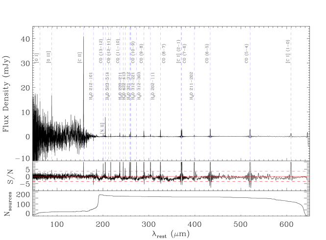
Figure 2.— Top: Average far-infrared stacked spectrum containing all data. Sources range in redshift from $0.005<z<4$. This stack serves as a qualitative representation of the average spectrum of all of the Herschel spectra. For the purposes of analysis and interpretation, the dataset is split into redshift and luminosity bins for the remainder of this paper. Dashed blue vertical lines indicate the locations of main molecular emission lines. We detect the fine-structure lines [C II], [O I], and [O III] as well as the CO emission line ladder from $J=13-12$ to $J=5-4$. Also detected are the two lowest [C I] emissions at 492 GHz (609 $\mu$m) and 809 GHz (370 $\mu$m), [N II] at 1461 GHz (205 $\mu$m) and the water lines within the frequency (wavelength) range covered in this stack from 50 $\mu$m to 652 $\mu$m). Middle: Signal-to-noise ratio. The horizontal dashed line indicates $\rm S/N=3.5$, and the solid red line represents $\rm S/N=0$. Bottom: The number of sources that contribute to the stack at each wavelength.

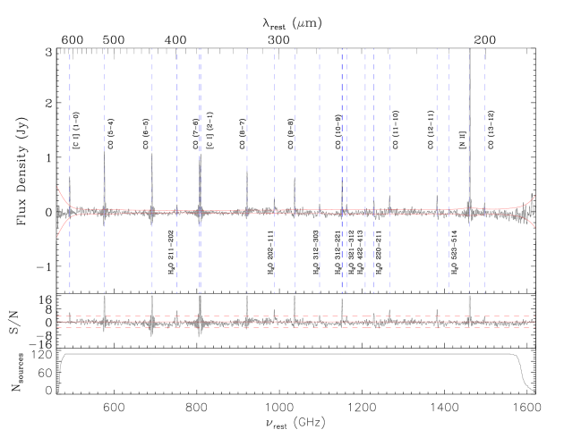
Figure 3.— Top: Stacked SPIRE/FTS spectrum of archival sources with $0.005<z<0.05$. Overlaid is the $1\sigma$ jackknifed noise level in red and dashed vertical lines showing the locations of main molecular emission lines. We detect the CO emission line ladder from $J=13-12$ to $J=5-4$, as well as the two lowest [C I] emissions at 492 GHz (609 $\mu$m) and 809 GHz (370 $\mu$m), [N II] at 1461 GHz (205 $\mu$m) and the water lines within the rest frequencies (wavelengths) covered in this stack from 460 GHz to 1620 GHz (185 $\mu$m to 652 $\mu$m). Middle: Signal-to-noise ratio. The horizontal dashed line indicates $\rm S/N=3.5$, and the solid red line indicates $\rm S/N=0$. Lines with $\rm S/N>3.5$ were considered detected. Bottom: The number of sources that contribute to the stack at each frequency.

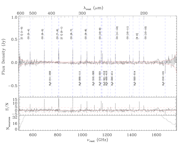
Figure 4.— Same as Figure 3, but for the redshift range $0.05<z<0.2$. We detect all the CO emission line ladder within the frequency (wavelength) covered by the stack from 480 GHz to 1760 GHz (170 $\mu$m to 625 $\mu$m). The stacked spectrum also shows 3.5$\sigma$ detection for $\rm[C\,I](2-1)$ at 809 GHz ($370\,\mu$m), [N II] at 1461 GHz (205 $\mu$m), and water lines.

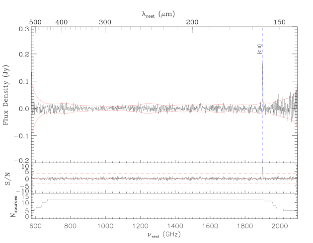
Figure 5.— Same as Figure 3, but for the redshift range $0.2<z<0.5$. We only detect the [C II] at 1901 GHz (158 $\mu$m) line in this stack with frequency (wavelength) coverage 580 GHz to 2100 GHz (143 $\mu$m to 517 $\mu$m).

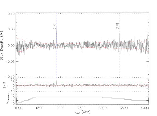
Figure 6.— Same as Figure 3, but for the redshift range $0.8<z<2$. We detect [N II] at 1461 GHz (205 $\mu$m), [C II] at 1901 GHz (158 $\mu$m) and [O III] at 3391 GHz (88 $\mu$m) in the frequency (wavelength) range of 950 GHz to 4100 GHz (70 $\mu$m to 316 $\mu$m) covered by the stack.

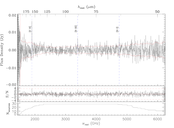
Figure 7.— Same as Figure 3, but for the redshift range $2<z<4$. We detect [C II] at 1901 GHz (158 $\mu$m) and [O III] at 3391 GHz (88 $\mu$m) in the frequency (wavelength) range of 1400 GHz to 6200 GHz (48 $\mu$m to 214 $\mu$m).

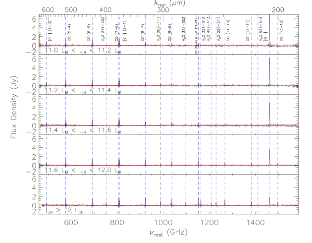
Figure 8.— The lowest redshift bin ($0.005<z<0.05$) is stacked using a straight mean (without inverse-variance weighting) in five luminosity bins as outlined in each panel. From top to bottom, the median luminosities in each bin are $10^{11.12}$ L_⊙, $10^{11.32}$ L_⊙, $10^{11.49}$ L_⊙, $10^{11.69}$ L_⊙, and $10^{12.21}$ L_⊙. The mean redshifts in each bin are 0.015, 0.018, 0.021, 0.027, and 0.038. The number of sources contributing to each bin are 37, 28, 17, 24, 9. and The CO molecular line excitations, [C I] atomic emissions, and [N II] at 205 $\mu$m are detected in all five luminosity bins.

2. Data

Despite the potential applications of mid- and far-IR spectral lines, the limited wavelength coverage and sensitivity of far-IR facilities have restricted the vast majority of observations to galaxies in the nearby universe. A significant leap came from the Herschel Space Observatory (Pilbratt et al., 2010), thanks to the spectroscopic capabilities of the Fourier Transform Spectrometer (FTS; Naylor et al. 2010; Swinyard et al. 2014) of the SPIRE instrument (Griffin et al., 2010). SPIRE covered the wavelength range of $194\,\rm{\mu m}-671\,\rm{\mu m}$, making it useful in the detection of ISM fine structure cooling lines, such as [C II] 158 $\rm{\mu m}$, [O III] 88 $\rm{\mu m}$, [N II] 205 $\rm{\mu m}$, and [O I] 63 $\rm{\mu m}$, in high-redshift galaxies and carbon monoxide (CO) and water lines (H₂O) from the ISM of nearby galaxies. The Herschel data archive contains SPIRE/FTS data for a total of 231 galaxies, with 197 known to be in the redshift interval $0.005<z<4.0$, completed through multiple programs either in guaranteed-time or open-time programs. While most of the galaxies at $0.5<z<4$ are intrinsically ultra-luminous IR galaxies (ULIRGS; Sanders & Mirabel 1996), with luminosities greater than $10^{12}\,$L_⊙, archival observations at $z>2$ are mainly limited to the brightest dusty starbursts with apparent L $>10^{13}\,$L_⊙ or hyper-luminous IR galaxies (HyLIRGs). Many of these cases, however, are gravitationally lensed DSFGs and their intrinsic luminosities are generally consistent with ULIRGS. At the lowest redshifts, especially in the range $0.005<z<0.05$, many of the targets have L $<10^{12}\,$L_⊙ or are luminous IR galaxies (LIRGs). While fine-structure lines are easily detected for such sources, most individual archival observations of brighter ULIRGs and HyLIRGs at $z>1$ do not reveal clear detections of far-infrared fine-structure lines despite their high intrinsic luminosities (George, 2015), except in a few very extreme cases such as the Cloverleaf quasar host galaxy (Uzgil et al., 2016). Thus, instead of individual spectra, we study the averaged stacked spectra of DSFGs, making use of the full SPIRE/FTS archive of Herschel.

Given the wavelength range of SPIRE and the redshifts of observed galaxies, to ease stacking, we subdivide the full sample of 197 galaxies into five redshift bins (Figure 1), namely, low-redshift galaxies at $0.005<z<0.05$ and $0.05<z<0.2$, intermediate redshifts $0.2<z<0.5$, and high-redshift galaxies at $0.8<z<2$ and $2<z<4$. Unfortunately, due to lack of published redshifts, we exclude observations of 24 targets or roughly 10% of the total archival sample (231 sources) from our stacking analysis expected to be mainly at $z>1$ based on the sample selection and flux densities. This is due to the fact that redshifts are crucial to shift spectra to a common redshift, usually taken to be the mean of the redshift distribution in each of our bins. For these 24 cases we also did not detect strong individual lines, which would allow us to establish a redshift conclusively with the SPIRE/FTS data. Most of these sources are likely to be at $z>1$ and we highlight this subsample in the Appendix to encourage follow-up observations. We also note that the SPIRE/FTS archive does not contain any observations of galaxies in the redshift interval of 0.5 to 0.8 and even in the range of $0.8<z<2$, observations are simply limited to 8 galaxies, compared to attempted observations of at least 28 galaxies, and possibly as high as 48 galaxies when including the subsample without redshifts, at $z>2$.

The data used in our analysis consist of 197 publicly-available Herschel   SPIRE/FTS spectra, as part of various Guaranteed Time (GT) and Open-Time (OT) Herschel programs summarized in the Appendix (Table LABEL:table:obsids). Detailed properties of the sample are also presented in the Appendix (Table LABEL:table:all_targets) for both low and high redshifts where the dividing line is at $z=0.8$, with 161 and 36 objects respectively. Table LABEL:table:all_targets also lists 34 sources at the end with existing FTS observations but which were not used in the analysis. The majority of unused sources have unknown or uncertain spectroscopic redshifts. This includes MACS J2043-2144 for which a single reliable redshift is currently uncertain as there is evidence for three galaxies with $z=2.040$, $z=3.25$, and $z=4.68$ within the SPIRE beam (Zavala et al., 2015). The sources SPT 0551-50 and SPT 0512-59 have known redshifts but do not have magnification factors. The low-redshift sample is restricted to DSFGs with $z>0.005$ only. This limits the bias in our stacked low-$z$ spectrum from bright near-by galaxies such as M81 and NGC 1068. Our selection does include bright sources such as Arp 220 and Mrk 231 in the stack, but we study their impact by breaking the lowest redshift sample into luminosity bins, including a ULIRG bin with L${}_{\rm IR}>10^{12}\,$L_⊙.

The Herschel sample of dusty, star-forming galaxies is composed of LIRGS with $10^{11}$ L${}_{\odot}\,<$ L $<10^{12}\,$L_⊙ and ULIRGS with L $>10^{12}\,$L_⊙. The sample is heterogeneous, consisting of AGN, starbursts, QSOs, LINERs, and Seyfert types 1 and 2. The low-redshift SPIRE/FTS spectra were taken as part of the HerCULES program (Rosenberg et al., 2015; PI van der Werf), HERUS program (Pearson et al., 2016; PI Farrah), and the Great Observatory All-Sky LIRG Survey (GOALS; Armus et al., 2009, Lu et al., 2017, PI: N. Lu) along with supplementary targets from the $\rm{KPGT\textunderscore wilso01\textunderscore 1}$ (PI: C. Wilson) and $\rm{OT2\textunderscore drigopou\textunderscore 3}$ (PI: D. Rigopoulou) programs. At $0.2<z<0.5$, the SPIRE/FTS sample of 11 galaxies is limited to Magdis et al. (2014), apart from one source, IRAS 00397-1312, from Helou & Walker (1988) and Farrah et al. (2007). Note that the Magdis et al. (2014) sample contained two galaxies initially identified to be at $z<0.5$, but later found to be background $z>2$ galaxies that were lensed by the $z<0.5$ foreground galaxy. Those data are included in our high-redshift sample.

The high-redshift sample at $z>0.8$ primarily comes from open-time programs that followed-up lensed galaxies from HerMES (Oliver et al., 2012) and H-ATLAS (Eales et al., 2010), and discussed in George (2015). Despite the boosting from lensing, only a few known cases of individual detections exist in the literature: NB.v1.43 at $z=1.68$ (George et al., 2013; Timmons et al., 2016), showing a clear signature of [C II] that led to a redshift determination for the first-time with a far-IR line, SMMJ2135-0102 (Cosmic eyelash; Ivison et al., 2010b), ID.81 and ID.9 (Negrello et al., 2014). With lens models for Herschel -selected lensed sources now in the literature (e.g., Bussmann et al., 2013; Calanog et al., 2014), the lensing magnification factors are now known with reasonable enough accuracy that the intrinsic luminosities of many of these high-redshift objects can be established. The $z>0.8$ sample is composed of 30 high-redshift, gravitationally-lensed galaxies (e.g., OT1_rivison_1, OT2_rivison_2) and 6 un-lensed galaxies (OT1_apope_2 and one each from OT1_rivison_1 and OT2_drigopou_3).

The distribution of redshifts can be found in Figure 1, where we have subdivided the total distribution into five redshift bins: $0.005<z<0.05$, $0.05<z<0.2$, $0.2<z<0.5$, $0.8<z<2$, and $2<z<4$. The mean redshifts in the five redshift bins are $z=0.02$, $z=0.1$, and $z=0.3$, $z=1.4$, and $z=2.8$, respectively. For reference, in Figure 1, we also show the $8-1000\,\mu$m luminosity distribution in the five redshift bins. The distribution spans mostly from LIRGS at low-redshifts to ULIRGS at $0.05<z<0.2$ and above. In the highest redshift bins we find ULIRGS again, despite increase in redshift, due to the fact that most of these are lensed sources; with magnification included, the observed sources will have apparent luminosities consistent with HyLIRGS. Unfortunately, there is a lack of data between redshifts of $z\sim 0.2$ and $z\sim 1$, with the Magdis et al. (2014) sample and the spectrum of IRAS 00397-1312 from HERUS (Pearson et al., 2016) being the only SPIRE/FTS observed spectra in this range.

In general, SPIRE/FTS observations we analyze here were taken in high resolution mode, with a spectral resolving power of $300-1000$ through a resolution of 1.2 GHz and frequency span of $\rm 447\,GHz-1568\,GHz$. The data come from two bolometer arrays: the spectrometer short wavelength (SSW) array, covering $\rm 194\,\mu m-318\,\mu m$ ($\rm 944\,GHz–1568\,GHz$) and the spectrometer long wavelength (SLW) array, covering $\rm 294\,\mu m-671\,\mu m$ ($\rm 447\,GHz–1018\,GHz$). The two arrays have different responses on the sky with the full-width half-maximum (FWHM) of the SSW beam at 18^′′ and the SLW beam varying from 30^′′ to 42^′′ with frequency (Swinyard et al., 2014). The SPIRE/FTS data typically involves $\sim 90-100$ scans of the faint, high-redshift sources and about half as many scans for the lower-redshift sources. Total integration times for each source are presented in Table LABEL:table:obsids. Typical total integration times of order 5000 seconds achieve unresolved spectral line sensitivities down to $\sim 10^{-18}\,{\rm W\,m^{-2}}(3\sigma)$.

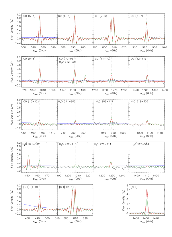
Figure 9.— Sinc-Gauss and sinc fits to the detected atomic and molecular lines in the low-redshift stack at $0.005<z<0.05$. The spectrum itself is shown in black. The green curve shows a sinc fit, red shows sinc-Gauss fit, and the blue curve is the 1$\sigma$ jackknife noise level. The sinc fit is often too thin to capture the full width of the spectral lines. The lines are shifted to the rest-frame based on the public spectroscopic redshifts reported in the literature. Fluxes are measured from the best-fit models. The fluxes of the lines are reported in Table 1.

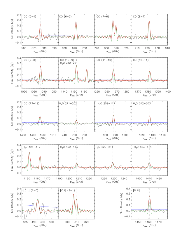
Figure 10.— Sinc-Gauss (red) and sinc (green) fits to the detected atomic and molecular lines in the stack at $0.05<z<0.2$, with the spectrum itself in black. We detect all the lines same as the low redshift stack (Figure 9) albeit with a different detection significance. In particular [C I] (1-0) is marginally detected in this redshift bin as fewer than ten sources contribute to the stack at this frequency, leading to a higher jackknife noise level. Fluxes of lines detected in this stack are also reported in Table 1.

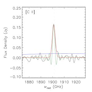
Figure 11.— Sinc-Gauss (red) and sinc (green) fits to the [C II] line in the $0.2<z<0.5$ stack. The spectrum itself is shown in black with the 1$\sigma$ noise level in blue.

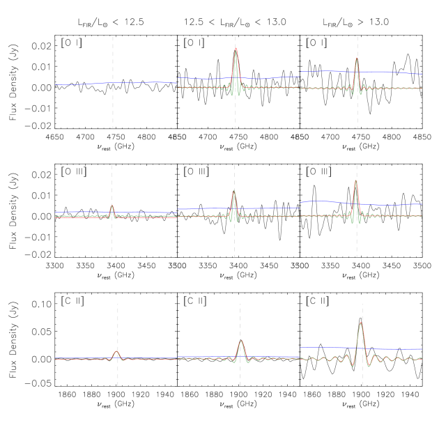
Figure 12.— Fits to lines for the three luminosity bins of the high-redshift sources. The sinc-Gauss fit is shown in red, and the sinc-only fit is shown in green. The spectrum itself in black, and the 1$\sigma$ jackknife noise level is in blue.

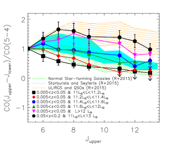
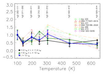
Figure 13.— Top: The carbon monoxide spectral line energy distribution for $0.005<z<0.05$ in five luminosity bins as presented in Figure 8. The filled regions are taken from Rosenberg et al. (2015) (see also Roberts-Borsani et al. 2017), and they correspond to the range of CO flux ratios in normal star-forming galaxies (green stripes), starbursts and Seyferts (solid cyan), and ULIRGs and QSOs (orange stripes). Bottom: Spectral line energy distribution for transitions in water as a function of excitation temperature as in Yang et al. (2013) at $0.005<z<0.05$ in the luminosity bins in which water lines were strongly detected. These detections are compared to the water spectral line energy distribution for individual sources fit using sinc-Gauss profiles.

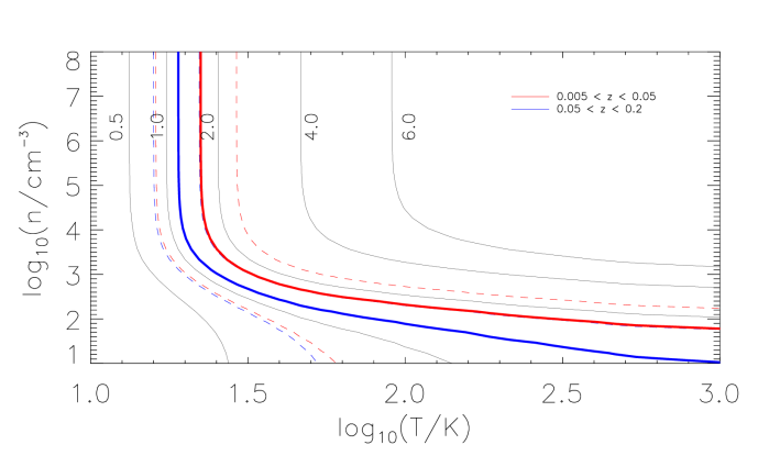
Figure 14.— Conditions in the ISM as probed by neutral [C I] (2-1)/[C I] (1-0) line ratio for $0.005<z<0.05$ and $0.05<z<0.2$ redshift bins. RADEX contours for an array of theoretical [C I] (2-1)/[C I] (1-0) ratios are shown in black. The dashed lines represent the 1$\sigma$ uncertainty.

3. Stacking Analysis

The Level-2 FTS spectral data are procured from the Herschel Science Archive (HSA) where they have already been reduced using version SPGv14.1.0 of the Herschel Interactive Processing Environment (HIPE, Ott (2010)) SPIRE spectrometer single pointing pipeline (Fulton et al., 2016) with calibration tree SPIRE_CAL_14_2. We use the point-source calibrated spectra. Additional steps are required to further reduce the data. An important step is the background subtraction. While Herschel/SPIRE-FTS observations include blank sky dark observations taken on or around the same observing day as the source observations are taken, they do not necessarily provide the best subtraction of the background (Pearson et al., 2016). The same study also showed that attempts to use a super-dark by combining many dark-sky observations into an average background do not always yield an acceptable removal of the background from science observations. Instead, the off-axis detectors present in each of the SPIRE arrays are used to construct a “dark” spectrum (Polehampton et al., 2015). These off-axis detectors provide multiple measurements of the sky and telescope spectra simultaneous with the science observations and are more effective at correcting the central spectrum. The background is constructed by taking the average of the off-axis detector spectra, but only after visually checking the spectra via HIPE’s background subtraction script (Polehampton et al., 2015) to ensure that the background detectors do not contain source emission. If any outliers are detected, they are removed from the analysis. Such outliers are mainly due to science observations that contain either an extended source or a random source that falls within the arrays. We use the average from all acceptable off-axis detectors from each science observation as the background to subtract from the central one. In a few unusual cases, a continuum bump from residual telescope emission in some spectra was better subtracted using a blank sky dark observation rather than an off-axis subtraction. In these cases, background subtraction was performed using the blank sky dark observation.

As part of the reduction, and similar to past analysis (e.g., Rosenberg et al. 2015; Pearson et al. 2016), we found a sizable fraction of the sources to show a clear discontinuity in flux between the continuum levels of the central SLW and SSW detectors in the overlap frequency interval between 944 GHz and 1018 GHz. If this discontinuity is still visible after the background subtraction (off-axis detector background or blank sky observation background) as discussed above, then we considered this offset to be an indication of extended source emission. For extended sources, we subtract a blank sky dark (and not an off-axis dark, as off-axis detectors may contain source emission) and correct for the source’s size with HIPE’s semiExtendedCorrector tool (SECT, Wu et al. 2013), following the Rosenberg et al. (2015) method of modeling the source as a Gaussian and normalizing the spectra for a Gaussian reference beam of 42^′′.

There are two other sources of discontinuity between the SLW and SSW detectors, one from a flux droop in the central SLW detector due to the recycling of the SPIRE cooler (Pearson et al., 2016) and another due to potential pointing offsets (Valtchanov et al., 2014). Due to the differences in the size of the SLW and SSW SPIRE beams, a pointing offset can cause a larger loss of flux in the SSW beam than in the SLW beam. If an extended source correction was not able to fix the discontinuity between the SLW and SSW detectors, the discontinuity may likely be coming from the cooler recycling or from a pointing offset. We assume that these two effects are negligible, as we remove any continuum remaining after the application of SECT from the central SLW and SSW detectors by subtracting a second-order polynomial fit to the continuum.

Once the corrected individual spectra are obtained, the high-redshift lensed sample was corrected for lensing magnification. The magnification factors come from lens models based on Sub-millimeter Array (SMA) and Keck/NIRC2-LGS adaptive optics observations (Bussmann et al., 2013; Calanog et al., 2014). Though these are mm-wave and optical magnifications while the present study involves far-IR observations, we ignore any effects of differential magnification (Serjeant, 2014). We simply make use of the best determined magnification factor, mainly from SMA analysis (Bussmann et al., 2013). For the overlapping lensed source sample with PACS spectroscopy, the lensing magnification factor used here is consistent with values used in Wardlow et al. (2017). Sources with PACS spectroscopy that appear in Wardlow et al. (2017) are marked in Table LABEL:table:all_targets.

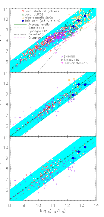
Figure 15.— Line versus infrared luminosity (rest-frame $8-1000\,\mu$m), L_IR, of star-forming galaxies for [C II], [O I], and [O III] fine structure lines at high redshift. Background data are from the literature sources listed in the text. The solid green lines correspond to the average L_line/L_IR ratios (-3.03, -2.94 and -2.84) for the [O I] 63.18 $\mu$m, [O III] 88.36 $\mu$m, and [C II] 157.7 $\mu$m lines from the literature, respectively. The reason for the choice of a linear relation is explained in the text. The cyan stripes correspond to two times the dispersion around the mean relation ($\sigma=0.35,0.48$ and $0.43$, respectively). Also shown, for comparison, are the $L_{\rm line}$/L_IR relations found in the literature (see text).

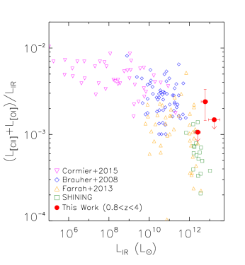
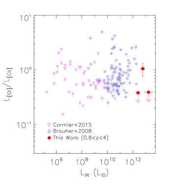
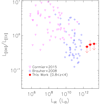
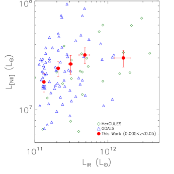
Figure 16.— Top Left: Ratio of ([C II]+[O I]) luminosity to total infrared luminosity (rest-frame $8-1000\,\mu$m) in three luminosity bins for sources with $0.8<z<4$ as a function of total infrared luminosity. The breakdown of the three luminosity bins is as follows: L${}_{\rm IR}<10^{12.5}\,$L_⊙, $10^{12.5}\,$L${}_{\odot}\,<$L${}_{\rm IR}<10^{13}\,$L_⊙, and L${}_{\rm IR}>10^{13}\,$L_⊙; however, [O I] is only detected in the middle luminosity bin. For comparison, we show data from Cormier et al. (2015); Brauher et al. (2008); Farrah et al. (2013) and Sturm et al. (2011b). Bottom Left and Top Right: Line ratios as a function of total infrared luminosity in three luminosity bins for sources with $0.8<z<4$. For comparison, we show data from Cormier et al. (2015) and Brauher et al. (2008). Right: Line luminosity of the [N II] transition in luminosity bins for sources at $0.005<z<0.05$. Background data were produced by fitting to the [NII] lines in individual spectra in the HerCULES and GOALS samples.

To obtain the average stacked spectrum in each of the redshift bins or luminosity bins as we discuss later we follow the stacking procedure outlined by Spilker et al. (2014). It involves scaling the flux densities in individual spectra in each redshift bin to the flux densities that the source would have were it located at some common redshift (which we take to be the mean redshift in each bin) and then scaling to a common luminosity so that we can present an average spectrum of the sample. For simplicity, we take the mean redshift and median infrared luminosity in each bin and both scale up and scale down individual galaxy spectra in both redshift and luminosity to avoid introducing biases in the average stacked spectrum; however we note that the sample does contain biases associated with initial sample selections in the proposals that were accepted for Herschel/SPIRE-FTS observations. We discuss how such selections impact a precise interpretation of the spectra in the discussion. We now outline the process used in the scaling of spectra.

The background-subtracted flux densities of the spectra are scaled to the flux values that they would have at the common redshift, which was taken to be the mean redshift in each of the redshift categories; namely, $z_{\rm com}=0.02$ for the $0.005<z<0.05$ sources, $z_{\rm com}=0.1$ for $0.05<z<0.2$ sources, $z_{\rm com}=0.3$ for $0.2<z<0.5$ sources, $z_{\rm com}=1.4$ for $0.8<z<2$ sources, and $z_{\rm com}=2.8$ for $2<z<4$ sources. The choice between median or mean redshift does not significantly affect the overall spectrum or line fluxes. The flux density and error values (error values are obtained from the error column of the level-2 spectrum products from the Herschel Science Archive) of each spectrum are multiplied by the scaling factor given in Spilker et al. (2014):

$$f=\bigg{(}\frac{D_{\rm L}(z_{\rm src})}{D_{\rm L}(z_{\rm com})}\bigg{)}^{2}\times\bigg{(}\frac{1+z_{\rm com}}{1+z_{\rm src}}\bigg{)}$$ (1)

where $D_{\rm L}$ is the luminosity distance. The flux density and error values of each spectrum are then representative of the flux density and error values that the source would have were it located at $z_{\rm com}$. The frequency axes of the scaled spectra are then converted from observed-frame frequencies to rest-frame frequencies.

To normalize the spectra, all spectrum flux densities and errors are scaled by a factor such that each source will have the same total infrared luminosity (rest-frame $8-1000\,\mu$m); namely, L${}_{\rm IR}=10^{11.35}\,$L_⊙, $10^{12.33}\,$L_⊙, $10^{11.89}\,$L_⊙, $10^{12.53}\,$L_⊙ and $10^{12.84}\,$L_⊙ in each of the five bins, respectively. In the two highest redshift bins, we calculate a total infrared luminosity by fitting a single-temperature, optically-thin, modified blackbody (i.e. greybody with $S({\nu})\propto\nu^{\beta}B_{\nu}(T)$ where $B_{\nu}(T)$ is the Planck function) spectral energy distribution (SED) (commonly used in the literature, e.g. Casey, 2012; Bussmann et al., 2013) to the available photometry in the infrared from Herschel and public IRSA data. For this we use the publicly available code developed by Casey (2012) assuming a fixed emissivity ($\beta=1.5$) (e.g. Bussmann et al., 2013). The resulting infrared luminosities are presented in Table LABEL:table:all_targets, along with lensing magnification factors and references. Luminosities in the tables are corrected for lensing magnification (where applicable), and we ignore the uncertainty in magnification from existing lens models. Sources without a magnification of factor $\mu$ are not affected by gravitational lensing.

After the spectra are scaled to a common IR luminosity, a second-order polynomial is then fit to the continuum of each source and is subsequently subtracted from each source spectrum. Instrumental noise impacts the continuum subtraction and leads to residuals in the continuum-subtracted spectrum. These residuals in return impact the detection of faint lines. A number of objects have multiple FTS spectra, taken at multiple time intervals as part of the same program or observations conducted in different programs. Multiples of the same object are combined into a single average spectrum by calculating the mean flux density at each frequency for each of the repeats. This mean spectrum is what is used in the stacking procedure. After the spectra are calibrated and scaled, the flux values at each frequency in the rest frame of the spectra are stacked using an inverse variance weighting scheme with the inverse of the square of the flux errors as weights. In the $0.005<z<0.05$ stack, a minority of the sources (though still a significant subset of the total) have high signal-to-noise ratios and thus dominate over the other sources when using the inverse variance weighting scheme. To avoid this bias without throwing out sources, we stack the $0.005<z<0.05$ bin by calculating the mean stack without inverse variance weighting. The unweighted mean stack is shown in Figure 3. The inverse variance weighted stack for this redshift bin is presented in the Appendix for comparison.

The noise level of the stacked spectrum in each of the five redshift bins is estimated using a jackknife technique in which we remove one source from the sample and then stack. The removed source is replaced, and this process is repeated for each source in the sample. The jackknife error in the mean of the flux densities at each frequency from the jackknifed stacks is taken to be the 1$\sigma$ noise level in the overall stacked spectrum in each redshift bin. The red curves in the upper panels of Figures 3 - 7 are found by smoothing the jackknife error curve.

4. Stacking Results

The stacked spectra in each of the five redshift bins are shown in Figures 3 - 7, while in Figure 8 we show the mean stacks (no inverse-variance weighting) for the $0.005<z<0.05$ bin by sub-dividing the sample into five luminosity bins given by $10^{11.0}\,$L${}_{\odot}<$ L${}_{\rm IR}<10^{11.2}\,$L_⊙, $10^{11.2}\,$L${}_{\odot}<$ L${}_{\rm IR}<10^{11.4}\,$L_⊙, $10^{11.4}\,$L${}_{\odot}<$ L${}_{\rm IR}<10^{11.6}\,$L_⊙, $10^{11.6}\,$L${}_{\odot}<$ L${}_{\rm IR}<10^{12.0}\,$L_⊙, and L${}_{\rm IR}>10^{12.0}\,$L_⊙. For the purposes of this study and for PDR model interpretations, we concentrate on lines that are detected at a signal-to-noise ratio greater than 3.5. The stacks do reveal detections with a signal-to-noise ratios at the level of 2.5 to 3; we will return to those lines in future papers.

The natural line shape of the SPIRE FTS is a sinc profile (Swinyard et al., 2014). A sinc profile is typically used to fit unresolved spectral lines. However, a sinc profile may be too thin to fully capture the width of broad partially-resolved extragalactic spectral lines, in which case a sinc-Gauss (sinc convolved with a Gaussian) can provide a better fit. For spectral lines with the same intrinsic line width, the sinc-Gauss fit gives a higher flux measurement than the sinc fit; the ratio of sinc-Gauss to sinc flux increases as a function of increasing spectral line frequency. For broad line-widths, the sinc-Gauss fit contains significantly more flux than the pure sinc fit. Because the stacked SPIRE/FTS spectra contain a variety of widths for each spectral line and because the width of each line is altered when scaling the frequency axis of the spectra to the common-redshift frame, the sinc profile appeared to under-fit all of the spectral lines in the stacked spectra, so a sinc-Gauss profile was used for flux extraction. See Figures 9 - 12. The width of the sinc component of the fit was fixed at the native SPIRE FTS resolution of 1.184 GHz, and the width of the Gaussian component was allowed to vary. The integral of the fitted sinc-Gauss profile was taken to be the measured flux. The fluxes from the fits are presented in Tables 1 - 3. In the case of an undetected line (i.e., the feature has less than 3.5$\sigma$ significance), we place an upper limit on its flux by injecting an artificial line with velocity width 300 km s^-1 (a typical velocity width for these lines; e.g., Magdis et al. 2014) into the stack at the expected frequency and varying the amplitude of this line until it is measured with 2$\sigma$ significance. The flux of this artificial line is taken to be the upper limit on the flux of the undetected line.

The error on the fluxes includes a contribution from the uncertainty in the fits to the spectral lines as well as a 6$\%$ uncertainty from the absolute calibration of the FTS. The error due to the fit is estimated by measuring the “bin-to-bin” spectral noise of the residual spectrum in the region around the line of interest (see SPIRE Data Reduction Guide). The residual spectrum is divided into bins with widths of 30 GHz, and the standard deviation of the flux densities within each bin is taken to be the noise level in that bin. Additionally, we incorporate a 15$\%$ uncertainty for corrections to the spectra for (semi)-extended sources (Rosenberg et al., 2015) in the lowest redshift stack. This 15% uncertainty is not included for sources with $z>0.05$, as these are all point sources (as verified by inspection).

We now discuss our stacking results for the five redshift bins; for simplicity we define low-redshift as $0.005<z<0.2$, intermediate as $0.2<z<0.5$ and high-redshift as $0.8<z<4$; both low and high-redshift have two additional redshift bins. Within these bins we also consider luminosity bins when adequate statistics allow us to further divide the samples.

4.1. Low-redshift stacks

Figures 3 and 4 show the stacked FTS spectra and corresponding uncertainty along with major atomic and molecular emission and absorption lines for the $0.005<z<0.05$ and $0.05<z<0.2$ bins respectively. With the large number of galaxy samples, the far-IR spectrum of lowest redshift bin results in a highly reliable average spectrum showing a number of ISM atomic and molecular emission lines. In particular we detect all the CO lines with $J_{\rm upper}>5$ out to the high excitation line of $\rm CO(13-12)$. This allows us to construct the CO spectral line energy distribution (SLED) and to explore the ISM excitation state in DSFGs in comparison with other starbursts and that of normal star-forming galaxies (see Section 5). We further detect multiple H₂O emission lines in these stacks which arise from the very dense regions in starbursts. The strength of the rotational water lines rivals that of the CO transition lines. We additionally detect the [C I] (1-0) at 609 $\mu$m and [C I] (2-1) at 370 $\mu$m along with [N II] at 205 $\mu$m in both redshift bins. We will use these measured line intensity ratios in Section 5 to construct photodissociation region models of the ISM and to study the density and ionizing photon intensities. We note here that the [C I] line ratios are very sensitive to the ISM conditions and would therefore not always agree with more simplistic models of the the ISM. We will discuss these further in Section 5. For comparison to Figure 3, which is stacked using an unweighted mean, Figure 20 shows the $0.005<z<0.05$ sources stacked with an inverse variance weighting. A few absorption lines also appear in the low-redshift stack. Despite Arp 220 (Rangwala et al., 2011) being the only individual source with strong absorption features, many of the absorption features are still present in the stack due to the high signal-to-noise ratio of Arp 220 in conjunction with an inverse variance weighting scheme for stacking. The SPIRE FTS spectrum of Arp 220 has been studied in detail in Rangwala et al. (2011) and is characterized by strong absorption features in water and related molecular ions OH⁺ and H₂O⁺ interpreted as a massive molecular outflow.

The best-fit profiles of the detected lines in the low-redshift stacks are shown in Figures 9 and 10 for the $0.005<z<0.05$ and $0.05<z<0.2$ redshift bins, respectively. Fluxes in $\rm{W\,m}^{-2}$ are obtained by integrating the best-fit line profiles. Table 1 summarizes these line fluxes as well as velocity-integrated fluxes from the sinc-Gauss fits for detections with $\rm S/N>3.5$ in these stacks.

As discussed above, we further stack the lowest redshift bin ($0.005<z<0.05$) in five infrared luminosity bins. Figure 8 shows the stacked FTS spectra each of these luminosity bins. See the caption in Figure 8 for the redshift and luminosity breakdown of the sample. By comparing these stacks we can look at the effects of infrared luminosity on emission line strengths. It appears from these stacked spectra that the high-$J$ CO lines are comparable in each of the luminosity bins. We explore the variation in the [N II] line in the discussion. Fluxes for the lines in each luminosity bin are tabulated in Figure 2.

4.2. Intermediate-redshift stacks

We show the intermediate-redshift ($0.2<z<0.5$) stack in Figure 5. Due to the limited number of galaxies observed with SPIRE/FTS in this redshift range, we only detect a bright [C II] line with our threshold signal-to-noise ratio of 3.5. The [C II] 158 $\mu$m fine structure line is a main ISM cooling line and is the most pronounced ISM emission line detectable at high redshifts, when it moves into mm bands, revealing valuable information on the state of the ISM. We further discuss these points in Section 5. Figure 11 shows the best-fit profile to the [C II] line in the intermediate redshift. The measured fluxes from this profile are reported in Table 1. The average [C II] flux from the stack is lower than the measurements reported in Magdis et al. (2014) for individual sources (note that our $0.2<z<0.5$ is comprised almost entirely of the sources from Magdis et al. (2014), the exception being the source IRAS 00397-1312). Stacking without IRAS 00397-1312 leads to similar results. We attribute the deviation of the stack [C II] flux toward lower values to the scalings we apply when shifting spectra to a common redshift and common luminosity during the stacking process.

4.3. High-redshift stacks

The high redshift ($0.8<z<2$ and $2<z<4$) FTS stacks are shown in Figures 6 and 7 consisting of 36 total individual spectra for sources in Table LABEL:table:all_targets. The stack at $0.8<z<2$ also suffers from a limited number of galaxies observed with the FTS. At $0.8<z<2$, [C II] 158 $\mu$m and [O III] 88 $\mu$m appear. We detect [C II] at 158 $\mu$m, [O III] at 88 $\mu$m and [O I] at 63 $\mu$m atomic emission lines with $\rm S/N>3.5$ in the stacked spectra at $2<z<4$. The relative line ratios of these main atomic fine structure cooling lines will be used to construct the photodissociation region model of the ISM of DSFGs at these extreme redshifts to investigate the molecular density and radiation intensity.

To study the strengths of spectral lines at different luminosities, all sources with $z>0.8$ were combined into a single sample and then divided into three luminosity bins with roughly the same number of sources in each bin. The average luminosities in the three bins are $10^{12.41}\,$L_⊙, $10^{12.77}\,$L_⊙, and $10^{13.24}\,$L_⊙. See Tables 3 and 4 for the precise breakdown of the sample and measured fluxes. Each of the subsamples is separately stacked, and the line fluxes are measured as a function of far-infrared luminosity. Figure 12 shows the best-fit line profiles to the three main detected emission lines in the three infrared luminosity bins. The ISM emission lines are more pronounced with increasing infrared luminosity. This agrees with results of individual detected atomic emission lines at high redshifts (Magdis et al., 2014; Riechers et al., 2014) although deviations from a main sequence are often observed depending on the physics of the ISM in the form of emission line deficits (Stacey et al., 2010). These are further discussed in the next section.

5. Discussion

The ISM atomic and molecular line emissions observed in the stacked spectra of DSFGs can be used to characterize the physical condition of the gas and radiation in the ISM across a wide redshift range. This involves investigating the CO and water molecular line transitions and the atomic line diagnostic ratios with respect to the underlying galaxy infrared luminosity for comparison to other populations and modeling of those line ratios to characterize the ISM.

5.1. The CO SLED

The CO molecular line emission intensity depends on the conditions in the ISM. Whereas the lower-$J$ CO emission traces the more extended cold molecular ISM, the high-$J$ emissions are observational evidence of ISM in more compact starburst clumps (e.g., Swinbank et al. 2011). In fact, observations of the relative strengths of the various CO lines have been attributed to a multi-phase ISM with different spatial extension and temperatures (Kamenetzky et al., 2016). The CO spectral line energy distribution (SLED), plotted as the relative intensity of the CO emission lines as a function of the rotational quantum number, $J$, hence reveals valuable information on the ISM conditions (e.g., Lu et al. 2014.

Figure 13 shows the high-$J$ CO SLED of the DSFGs for stacks in the two low redshift bins of $0.005<z<0.05$ and $0.05<z<0.2$. Here we are limited to the $J_{\rm upper}>5$ CO SLED covered by the SPIRE/FTS in the redshift range probed. A combined Herschel/SPIRE and PACS stacked spectra of DSFGs and corresponding full CO SLED will be presented in Wilson et al. in prep. The CO SLED is normalized to CO (5-4) line flux density and plotted as a function of ${J_{\rm upper}}$. The background colored regions in 13 are from Rosenberg et al. (2015) in which they determined a range of CO flux ratios for three classes of galaxies from the HerCULES sample: star-forming objects, starbursts and Seyferts, and ULIRGs and QSOs. The $0.005<z<0.05$ sample is consistent with the starbursts and Seyfert regions whereas line measurements from stacked spectra in $0.05<z<0.2$ redshift bin are more consistent with ULIRGs and QSO regions. Both measurements are higher than the expected region for normal star-forming galaxies which indicates a heightened excitation state in DSFGs specifically at the high-$J$ lines linked to stronger radiation from starbursts and/or QSO activity.

Increased star-formation activity in galaxies is often accompanied by an increase in the molecular gas reservoirs. This is studied locally as a direct correlation between the observed infrared luminosity and CO molecular gas emission in individual LIRGs and ULIRGs (Kennicutt & Evans, 2012). To further investigate this correlation, we looked at the CO SLED in our low-$z$ ($0.005<z<0.05$) sample in bins of infrared luminosity (Figure 8). Figure 13 further shows the CO SLED for the the different luminosity bins. The stronger radiation present in the higher luminosity bin sample, as traced by the total infrared luminosity, is responsible for the increase in the CO line intensities. In the high luminosity bin sample, the excitation of the high-$J$ lines could also partially be driven by AGN activity given the larger fraction of QSO host galaxies in the most IR luminous sources (e.g., Rosenberg et al. 2015).

5.2. ISM Emission Lines

5.2.1 Atomic and Molecular Line Ratios

We detect several $\rm H_{2}O$ emission lines in the two lowest redshift bins of $0.005<z<0.05$ and $0.05<z<0.2$. Fluxes from detected water rotational lines are plotted in Figure 13, along with data from fits made to individual spectra from the sample that exhibited strong water line emission. These include well-known sources such as Arp 220 at $z=0.0181$ (Rangwala et al., 2011) and Mrk 231 at $z=0.0422$ (van der Werf et al., 2010; González-Alfonso et al., 2010a). $\rm H_{2}O$ lines are normally produced in the warm and most dense regions of starbursts (Danielson et al., 2011) and may indicate infrared pumping by AGN (González-Alfonso et al., 2010b; Bradford et al., 2011). Figure 13 also shows the different water emission lines and the ISM temperatures required for their production. As we see from the figure, at the highest temperature end the emission is more pronounced in galaxies in the $0.05<z<0.2$ redshift range. These systems tend to have a higher median infrared luminosity (Figure 1) and hence hotter ISM temperatures which are believed to drive the high temperature water emissions (Takahashi et al., 1983). Figure 13 also shows the dependence of the water emission lines on the infrared luminosity for three of our five luminosity bins in the $0.005<z<0.05$ sample with the strongest H₂O detections. Using a sample of local Herschel FTS/SPIRE spectra with individual detections, Yang et al. (2013) showed a close to linear relation between the strength of water lines and that of L_IR. We observe a similar relation in our stacked binned water spectra of DSFGs across all different transitions with higher water emission line intensities in the more IR-luminous sample.

The first two neutral [C I] transitions ([C I] (1-0) at 609 $\mu$m and [C I] (2-1) at 370 $\mu$m) are detected in both low-$z$ stacks (see Figures 3 and 4). We look at the [C I] line ratios in terms of gas density and kinetic temperature using the non-LTE radiative transfer code RADEX (van der Tak et al., 2007). To construct the RADEX models, we use the collisional rate coefficients by Schroder et al. (1991) and use the same range of ISM physical conditions reported in Pereira-Santaella et al. (2013) (with $T=10-1000\,{\rm K}$, $n_{\rm H_{2}}=10-10^{8}\,{\rm cm^{-3}}$ and $N_{\rm C}/\Delta v=10^{12}-10^{18}\,{\rm cm^{-2}/(km\,s^{-1})}$). Figure 14 shows the expected kinetic temperature and molecular hydrogen density derived by RADEX for the observed [C I] ratios in the low-$z$ stacks for the different infrared luminosity bins with contours showing the different models. The [C I] emission is observed to originate from the colder ISM traced by CO (1-0) rather than the warm molecular gas component traced by the high-$J$ CO lines (Pereira-Santaella et al., 2013) and in fact the temperature is well constrained from these diagrams for high gas densities.

The fine structure emission line relative strengths are important diagnostics of the physical conditions in the ISM. Here we focus on the three main atomic lines detected at $z>0.8$ ([C II] at 158 $\mu$m, [O I] at 63 $\mu$m and [O III] at 88 $\mu$m) and study their relative strengths as well as their strength in comparison to the infrared luminosity of the galaxy. We break all sources with $z>0.8$ into three smaller bins based on total infrared luminosity. Table 4 lists the infrared luminosity bins used. The [C II] line is detected in each subset of the high-redshift stack whereas [O I] and [O III] are only detected in the $10^{12.5}$ L_⊙ $<$ $10^{13}$ L_⊙ infrared luminosity bin.

Figure 15 shows the relation between emission line luminosity and total infrared luminosity. Total infrared luminosity is integrated in the rest-frame wavelength range $8-1000\,\mu$m. Luminosities in different wavelength ranges in the literature have been converted to L_IR using the mean factors derived from Table 7 of Brisbin et al. (2015):

$${\rm log}(\rm{L}_{\rm IR})={\rm log}(\rm{L}(42.5\,\mu{\rm m}-122.5\,\mu{\rm m}))+0.30$$ (2a)

$${\rm log}(\rm{L}_{\rm IR})={\rm log}(\rm{L}(40\,\mu{\rm m}-500\,\mu{\rm m}))+0.145$$ (2b)

$${\rm log}(\rm{L}_{\rm IR})={\rm log}(\rm{L}(30\,\mu{\rm m}-1000\,\mu{\rm m}))+0.09$$ (2c)

For the [C II] 158 $\mu$m line we used data from a compilation by Bonato et al. (2014); references therein, George (2015), Brisbin et al. (2015), Oteo et al. (2016), Gullberg et al. (2015), Schaerer et al. (2015), Yun et al. (2015), Magdis et al. (2014), Farrah et al. (2013), Stacey et al. (2010), Díaz-Santos et al. (2013), and a compilation of data from SHINING (Sturm et al., 2011b). For the [O I] 63 $\mu$m line we used data from compilation by Bonato et al. (2014); references therein, Ferkinhoff et al. (2014), Brisbin et al. (2015), Farrah et al. (2013), and SHINING (Sturm et al., 2011b). For the [O III] 88 $\mu$m line we used data from a compilation by Bonato et al. (2014); references therein, George (2015), and SHINING (Sturm et al., 2011b). As in Bonato et al. (2014), we excluded all objects for which there is evidence for a substantial AGN contribution. The line and continuum measurements of strongly lensed galaxies given by George (2015) were corrected using the gravitational magnifications, $\mu$, estimated by Ferkinhoff et al. (2014) while those by Gullberg et al. (2015) were corrected using the magnification estimates from Hezaveh et al. (2013) and Spilker et al. (2016) available for 17 out of the 20 sources. For the other three sources we used the median value of $\mu_{\rm med}$ = 7.4. The solid green lines in Figure 15 correspond to the average L_line/L_IR ratios of -3.03, -2.94 and -2.84 for the [O I] 63 $\mu$m, [O III] 88 $\mu$m and [C II] 158 $\mu$m lines from the literature, respectively. The [CII] line luminosity-to-IR luminosity ratio is at least an order of magnitude higher than the typical value of 10^-4 quoted in the literature for local nuclear starburst ULIRGS and high-z QSOs.

Since the data come from heterogeneous samples, a least square fitting is susceptible to selection effects that may bias the results. To address this issue, Bonato et al. (2014) have carried out an extensive set of simulations of the expected emission line intensities as a function of infrared luminosity for different properties (density, metallicity, filling factor) of the emitting gas, different ages of the stellar populations and a range of dust obscuration. For a set of lines, including those considered in this paper the simulations were consistent with a direct proportionality between L_line and L_IR. Based on this result, we have adopted a linear relation. The other lines show L${}_{\rm line}-$L_IR relations found in the literature, namely:

$${\rm log}(\rm{L}{\rm[O\,I]}\,63\,\mu{\rm m})={\rm log}(\rm{L}_{\rm IR})-2.99,$$ (3a)

$${\rm log}(\rm{L}{\rm[O\,III]}\,88\,\mu{\rm m})={\rm log}(\rm{L}_{\rm IR})-2.87,$$ (3b)

$${\rm log}(\rm{L}{\rm[C\,II]}\,158\,\mu{\rm m})={\rm log}(\rm{L}_{\rm IR})-2.74,$$ (3c)

from Bonato et al. (2014),

$${\rm log}(\rm{L}{\rm[O\,I]}\,63\,\mu{\rm m})=0.98\times{\rm log}(\rm{L}_{\rm IR})-2.95,$$ (4a)

$${\rm log}(\rm{L}{\rm[O\,III]}\,88\,\mu{\rm m})=0.98\times{\rm log}(\rm{L}_{\rm IR})-3.11,$$ (4b)

$${\rm log}(\rm{L}{\rm[C\,II]}\,158\,\mu{\rm m})=0.89\times{\rm log}(\rm{L}_{\rm IR})-2.67,$$ (4c)

from Spinoglio et al. (2014),

$${\rm log}(\rm{L}{\rm[O\,I]}\,63\,\mu{\rm m})=0.70\times{\rm log}(\rm{L}_{\rm IR})+0.32,$$ (5a)

$${\rm log}(\rm{L}{\rm[O\,III]}\,88\,\mu{\rm m})=0.82\times{\rm log}(\rm{L}_{\rm IR})-1.40,$$ (5b)

$${\rm log}(\rm{L}{\rm[C\,II]}\,158\,\mu{\rm m})=0.94\times{\rm log}(\rm{L}_{\rm IR})-2.39,$$ (5c)

from Gruppioni et al. (2016), and

$${\rm log}(\rm{L}{\rm[O\,I]}\,63\,\mu{\rm m})=1.10\times{\rm log}(\rm{L}_{\rm IR})-4.70,$$ (6a)

$${\rm log}(\rm{L}{\rm[C\,II]}\,158\,\mu{\rm m})=1.56\times{\rm log}(\rm{L}_{\rm IR})-10.52,$$ (6b)

from Farrah et al. (2013), respectively.

In the high-$z$ bin at $z>1$, we find that [O III] and [O I] detections are limited to only one of the three luminosity bins. The ISM emission lines show a deficit (i.e. deviating from a one to one relation) compared to the infrared luminosity. This in particular is more pronounced in our stacked high-$z$ DSFG sample compared to that of local starbursts and is similar to what is observed in local ULIRGs. This deficit further points towards an increase in the atomic ISM lines optical depth in these very dusty environments. There is no clear trend in the measured lines with the infrared luminosities, given the measured uncertainties, however there is some evidence pointing towards a further decrease with increasing IR luminosity. Figure 16 shows the [O I]/[C II] line ratio for the stacks of DSFGs compared to Brauher et al. (2008) and Cormier et al. (2015). Although both lines trace neutral gas, they have different excitation energies (with the [O I] being higher). Given the uncertainties, we don’t see a significant trend in this line ratio with the infrared luminosity.

Due to the wavelength coverage of SPIRE/FTS, we are unable to study the [N II] 205 $\mu$m line in the high-$z$ bin. Instead, we concentrate on the luminosity dependence of the [N II] 205 $\mu$m line in the low-$z$ bin. This [N II] ISM emission cooling line is usually optically thin, suffering less dust attenuation compared to optical lines and hence is a strong star-formation rate indicator (Zhao et al., 2013; Herrera-Camus et al., 2016; Hughes et al., 2016; Zhao et al., 2016). The [N II] line luminosity in fact shows a tight correlation with SFR for various samples of ULIRGs (Zhao et al., 2013). Given the ionization potential of [N II] at 14.53 eV, this line is also a good tracer of the warm ionized ISM regions (Zhao et al., 2016). Figure 16 shows the [N II] emission for our low-$z$ stack ($0.005<z<0.05$) as a function of infrared luminosity for the five luminosity bins outlined in Figure 8. The [N II] line luminosity probes the same range as observed for other samples of ULIRGs and consistently increases with infrared luminosity (a proxy for star-formation) (Zhao et al., 2013). The [N II]/L_IR ratio is $\sim 10^{-5}$ compared to the [C II]/L_IR at $\sim 10^{-3}$ (Díaz-Santos et al., 2013; Ota et al., 2014; Herrera-Camus et al., 2015; Rosenberg et al., 2015).

Table 1Fluxes of observed spectral lines in each of the redshift bins.

		$0.005<z<0.05$		$0.05<z<0.2$		$0.2<z<0.5$		$0.8<z<2$		$2<z<4$
Line	Rest Freq.	Flux	Flux	Flux	Flux	Flux	Flux	Flux	Flux	Flux	Flux
	[$\rm{GHz}$]	[$10^{-18}$ $\rm{W}\rm{m^{-2}}$]	[$\rm{Jy}\,\rm{km}\,\rm{s^{-1}}$]	[$10^{-18}$ $\rm{W}\rm{m^{-2}}$]	[$\rm{Jy}\,\rm{km}\,\rm{s^{-1}}$]	[$10^{-18}$ $\rm{W}\rm{m^{-2}}$]	[$\rm{Jy}\,\rm{km}\,\rm{s^{-1}}$]	[$10^{-18}$ $\rm{W}\rm{m^{-2}}$]	[$\rm{Jy}\,\rm{km}\,\rm{s^{-1}}$]	[$10^{-18}$ $\rm{W}\rm{m^{-2}}$]	[$\rm{Jy}\,\rm{km}\,\rm{s^{-1}}$]
CO (5-4)	576.268	15 $\pm$ 3	790 $\pm$ 130	2.8 $\pm$ 0.4	160 $\pm$ 30	-	-	-	-	-	-
CO (6-5)	691.473	14 $\pm$ 3	620 $\pm$ 100	3.8 $\pm$ 0.4	180 $\pm$ 20	$<$ 0.40	$<$ 23	-	-	-	-
CO (7-6)	806.653	12 $\pm$ 2	440 $\pm$ 80	4.7 $\pm$ 0.4	190 $\pm$ 20	$<$ 0.38	$<$ 19	-	-	-	-
CO (8-7)	921.800	11 $\pm$ 2	360 $\pm$ 60	4.5 $\pm$ 0.4	160 $\pm$ 20	$<$ 0.24	$<$ 10	-	-	-	-
CO (9-8)	1036.914	9.7 $\pm$ 1.7	280 $\pm$ 50	4.0 $\pm$ 0.5	130 $\pm$ 20	$<$ 0.21	$<$ 7.7	$<$ 0.48	$<$ 33	-	-
CO (10-9)	1151.985	9.6 $\pm$ 1.7	250 $\pm$ 50	5.7 $\pm$ 0.6	160 $\pm$ 20	$<$ 0.32	$<$ 11	$<$ 0.34	$<$ 21	-	-
CO (11-10)	1267.016	4.9 $\pm$ 1.0	120 $\pm$ 30	3.9 $\pm$ 0.4	100 $\pm$ 20	$<$ 0.50	$<$ 16	$<$ 0.21	$<$ 12	-	-
CO (12-11)	1381.997	5.4 $\pm$ 1.1	120 $\pm$ 30	3.5 $\pm$ 0.5	84 $\pm$ 10	$<$ 0.34	$<$ 9.5	$<$ 0.26	$<$ 14	-	-
CO (13-12)	1496.926	2.3 $\pm$ 0.6	54 $\pm$ 13	2.7 $\pm$ 0.5	60 $\pm$ 9	$<$ 0.37	$<$ 9.7	$<$ 0.33	$<$ 16	$<$ 0.38	$<$ 29
$\rm{H_{2}O}$ 211-202	752.032	1.9 $\pm$ 0.4	78 $\pm$ 17	1.1 $\pm$ 0.3	49 $\pm$ 9	$<$ 0.49	$<$ 26	-	-	-	-
$\rm{H_{2}O}$ 202-111	987.927	5.5 $\pm$ 1.2	170 $\pm$ 40	2.3 $\pm$ 0.3	78 $\pm$ 9	$<$ 0.30	$<$ 12	$<$ 0.50	$<$ 37	-	-
$\rm{H_{2}O}$ 312-303	1097.365	2.7 $\pm$ 0.7	75 $\pm$ 19	2.3 $\pm$ 0.3	70 $\pm$ 9	$<$ 0.23	$<$ 8.2	$<$ 0.43	$<$ 29	-	-
$\rm{H_{2}O}$ 312-221	1153.128	-	-	-	-	-	-	-	-	-	-
$\rm{H_{2}O}$ 321-312	1162.910	2.7 $\pm$ 0.7	72 $\pm$ 18	2.9 $\pm$ 0.3	82 $\pm$ 9	$<$ 0.32	$<$ 11	$<$ 0.31	$<$ 19	-	-
$\rm{H_{2}O}$ 422-413	1207.638	$<$ 1.2	$<$ 30	1.6 $\pm$ 0.5	44 $\pm$ 12	$<$ 0.42	$<$ 14	$<$ 0.25	$<$ 15	-	-
$\rm{H_{2}O}$ 220-211	1228.789	3.9 $\pm$ 1.0	96 $\pm$ 23	1.6 $\pm$ 0.4	43 $\pm$ 11	$<$ 0.50	$<$ 16	$<$ 0.24	$<$ 14	-	-
$\rm{H_{2}O}$ 523-514	1410.615	$<$ 1.4	$<$ 30	1.8 $\pm$ 0.4	41 $\pm$ 9	$<$ 0.35	$<$ 9.7	$<$ 0.36	$<$ 19	-	-
$[\rm C\,I]\,(1-0)$	492.161	9.2 $\pm$ 4.1	570 $\pm$ 250	2.5 $\pm$ 0.8	170 $\pm$ 50	-	-	-	-	-	-
$[\rm C\,I]\,(2-1)$	809.340	15 $\pm$ 3	570 $\pm$ 100	3.0 $\pm$ 0.3	120 $\pm$ 10	$<$ 0.39	$<$ 18	-	-	-	-
$[\rm N\,II]$	1461.132	96 $\pm$ 16	2000 $\pm$ 400	5.4 $\pm$ 0.5	120 $\pm$ 10	$<$ 0.39	$<$ 11	$<$ 0.14	$<$ 6.9	$<$ 0.52	$<$ 41
$[\rm C\,II]$	1901.128	-	-	-	-	4.0 $\pm$ 0.4	83 $\pm$ 7	1.3 $\pm$ 0.2	51 $\pm$ 5	0.22 $\pm$ 0.04	13 $\pm$ 2
$[\rm N\,II]$	2461.250	-	-	-	-	-	-	$<$ 0.17	$<$ 4.8	$<$ 0.048	$<$ 2.2
$[\rm O\,III]$	3393.006	-	-	-	-	-	-	1.1 $\pm$ 0.3	23 $\pm$ 6	0.14 $\pm$ 0.03	4.5 $\pm$ 1.0
$[\rm O\,I]$	4744.678	-	-	-	-	-	-	-	-	0.14 $\pm$ 0.05	3.5 $\pm$ 1.1

Table 2 Measured fluxes of observed spectral lines from sources with $0.005<z<0.05$ in five luminosity bins.

		$10^{11.0}\,$L${}_{\odot}\,<$ L $<10^{11.2}\,$L⊙		$10^{11.2}\,$L${}_{\odot}\,<$ L $<10^{11.4}\,$L⊙		$10^{11.4}\,$L${}_{\odot}\,<$ L $<10^{11.6}\,$L⊙		$10^{11.6}\,$L${}_{\odot}\,<$ L $<10^{12.0}\,$L⊙		L $>10^{12.0}\,$L⊙
Line	Rest Freq.	Flux	Flux	Flux	Flux	Flux	Flux	Flux	Flux	Flux	Flux
	[$\rm{GHz}$]	[$10^{-18}$ $\rm{W}\rm{m^{-2}}$]	[$\rm{Jy}\,\rm{km}\,\rm{s^{-1}}$]	[$10^{-18}$ $\rm{W}\rm{m^{-2}}$]	[$\rm{Jy}\,\rm{km}\,\rm{s^{-1}}$]	[$10^{-18}$ $\rm{W}\rm{m^{-2}}$]	[$\rm{Jy}\,\rm{km}\,\rm{s^{-1}}$]	[$10^{-18}$ $\rm{W}\rm{m^{-2}}$]	[$\rm{Jy}\,\rm{km}\,\rm{s^{-1}}$]	[$10^{-18}$ $\rm{W}\rm{m^{-2}}$]	[$\rm{Jy}\,\rm{km}\,\rm{s^{-1}}$]
CO (5-4)	576.268	22 $\pm$ 4	1200 $\pm$ 200	17 $\pm$ 3	880 $\pm$ 150	16 $\pm$ 3	840 $\pm$ 150	20 $\pm$ 4	1100 $\pm$ 200	18 $\pm$ 4	980 $\pm$ 170
CO (6-5)	691.473	16 $\pm$ 3	720 $\pm$ 120	16 $\pm$ 3	710 $\pm$ 120	18 $\pm$ 3	820 $\pm$ 150	20 $\pm$ 4	910 $\pm$ 200	22 $\pm$ 4	1000 $\pm$ 200
CO (7-6)	806.653	13 $\pm$ 3	480 $\pm$ 80	12 $\pm$ 3	470 $\pm$ 80	15 $\pm$ 3	580 $\pm$ 100	20 $\pm$ 4	760 $\pm$ 130	24 $\pm$ 4	910 $\pm$ 150
CO (8-7)	921.800	10 $\pm$ 2	330 $\pm$ 60	11 $\pm$ 2	370 $\pm$ 70	15 $\pm$ 3	500 $\pm$ 90	19 $\pm$ 3	630 $\pm$ 110	27 $\pm$ 5	930 $\pm$ 160
CO (9-8)	1036.914	8.5 $\pm$ 2.0	250 $\pm$ 60	7.7 $\pm$ 1.7	230 $\pm$ 50	14 $\pm$ 3	410 $\pm$ 80	16 $\pm$ 3	490 $\pm$ 90	24 $\pm$ 5	730 $\pm$ 130
CO (10-9)	1151.985	8.5 $\pm$ 1.9	230 $\pm$ 50	10 $\pm$ 2	260 $\pm$ 50	14 $\pm$ 4	380 $\pm$ 90	17 $\pm$ 3	460 $\pm$ 80	34 $\pm$ 6	930 $\pm$ 160
CO (11-10)	1267.016	$<$ 7.0	$<$ 170	3.4 $\pm$ 1.2	82 $\pm$ 27	12 $\pm$ 4	290 $\pm$ 100	10 $\pm$ 2	250 $\pm$ 50	21 $\pm$ 4	520 $\pm$ 90
CO (12-11)	1381.997	$<$ 5.0	$<$ 110	4.6 $\pm$ 1.5	100 $\pm$ 30	6.4 $\pm$ 1.9	140 $\pm$ 40	11 $\pm$ 2	250 $\pm$ 50	14 $\pm$ 3	320 $\pm$ 60
CO (13-12)	1496.926	$<$ 3.9	$<$ 80	$<$ 4.8	$<$ 97	$<$ 9.3	$<$ 190	11 $\pm$ 3	220 $\pm$ 50	15 $\pm$ 3	310 $\pm$ 60
$\rm{H_{2}O}$ 211-202	752.032	$<$ 1.5	$<$ 59	2.4 $\pm$ 0.6	97 $\pm$ 25	5.2 $\pm$ 1.4	210 $\pm$ 60	3.0 $\pm$ 0.6	120 $\pm$ 30	9.3 $\pm$ 1.7	390 $\pm$ 70
$\rm{H_{2}O}$ 202-111	987.927	$<$ 3.2	$<$ 99	5.4 $\pm$ 1.2	170 $\pm$ 40	$<$ 6.1	$<$ 190	4.8 $\pm$ 1.1	150 $\pm$ 40	18 $\pm$ 4	580 $\pm$ 110
$\rm{H_{2}O}$ 312-303	1097.365	$<$ 6.1	$<$ 170	$<$ 3.2	$<$ 88	$<$ 5.9	$<$ 170	$<$ 4.8	$<$ 140	12 $\pm$ 3	350 $\pm$ 70
$\rm{H_{2}O}$ 312-221	1153.128	-	-	-	-	-	-	-	-	-	-
$\rm{H_{2}O}$ 321-312	1162.910	$<$ 2.7	$<$ 69	3.5 $\pm$ 1.1	93 $\pm$ 28	$<$ 5.0	$<$ 140	3.8 $\pm$ 1.1	100 $\pm$ 30	19 $\pm$ 4	520 $\pm$ 90
$\rm{H_{2}O}$ 422-413	1207.638	$<$ 2.7	$<$ 67	$<$ 2.4	$<$ 60	$<$ 2.7	$<$ 68	$<$ 3.4	$<$ 87	8.6 $\pm$ 1.9	220 $\pm$ 50
$\rm{H_{2}O}$ 220-211	1228.789	$<$ 4.6	$<$ 120	4.6 $\pm$ 1.5	110 $\pm$ 37	6.1 $\pm$ 1.9	150 $\pm$ 50	3.0 $\pm$ 0.9	75 $\pm$ 22	16 $\pm$ 3	400 $\pm$ 80
$\rm{H_{2}O}$ 523-514	1410.615	$<$ 3.0	$<$ 65	$<$ 3.6	$<$ 77	$<$ 2.8	$<$ 61	$<$ 1.8	$<$ 40	7.5 $\pm$ 1.9	170 $\pm$ 40
$[\rm C\,I]\,(1-0)$	492.161	14 $\pm$ 5	850 $\pm$ 250	11 $\pm$ 3	680 $\pm$ 140	10 $\pm$ 3	640 $\pm$ 150	9.6 $\pm$ 2.3	600 $\pm$ 140	8.8 $\pm$ 2.7	560 $\pm$ 170
$[\rm C\,I]\,(2-1)$	809.340	21 $\pm$ 4	790 $\pm$ 130	19 $\pm$ 4	700 $\pm$ 120	20 $\pm$ 4	750 $\pm$ 130	17 $\pm$ 3	640 $\pm$ 110	16 $\pm$ 3	610 $\pm$ 110
$[\rm N\,II]$	1461.132	160 $\pm$ 30	3300 $\pm$ 600	130 $\pm$ 20	2600 $\pm$ 500	100 $\pm$ 20	2100 $\pm$ 400	73 $\pm$ 12	1500 $\pm$ 300	34 $\pm$ 6	730 $\pm$ 120
$[\rm C\,II]$	1901.128	-	-	-	-	-	-	-	-	-	-
$[\rm N\,II]$	2461.250	-	-	-	-	-	-	-	-	-	-
$[\rm O\,III]$	3393.006	-	-	-	-	-	-	-	-	-	-
$[\rm O\,I]$	4744.678	-	-	-	-	-	-	-	-	-	-

Table 3Measured fluxes of observed spectral lines from sources with $0.8<z<4$ in three luminosity bins.

		$10^{11.5}\,$L${}_{\odot}\,<$ L $<10^{12.5}\,$L⊙		$10^{12.5}\,$L${}_{\odot}\,<$ L $<10^{13.0}\,$L⊙		$10^{13.0}\,$L${}_{\odot}\,<$ L $<10^{14.5}\,$L⊙
Line	Rest Freq.	Flux	Flux	Flux	Flux	Flux	Flux
	[$\rm{GHz}$]	[$10^{-18}$ $\rm{W}\rm{m^{-2}}$]	[$\rm{Jy}\,\rm{km}\,\rm{s^{-1}}$]	[$10^{-18}$ $\rm{W}\rm{m^{-2}}$]	[$\rm{Jy}\,\rm{km}\,\rm{s^{-1}}$]	[$10^{-18}$ $\rm{W}\rm{m^{-2}}$]	[$\rm{Jy}\,\rm{km}\,\rm{s^{-1}}$]
CO (5-4)	576.268	-	-	-	-	-	-
CO (6-5)	691.473	-	-	-	-	-	-
CO (7-6)	806.653	-	-	-	-	-	-
CO (8-7)	921.800	-	-	-	-	-	-
CO (9-8)	1036.914	$<$ 1.5	$<$ 130	-	-	-	-
CO (10-9)	1151.985	$<$ 1.1	$<$ 89	$<$ 0.51	$<$ 46	-	-
CO (11-10)	1267.016	$<$ 0.66	$<$ 50	$<$ 0.21	$<$ 17	-	-
CO (12-11)	1381.997	$<$ 0.18	$<$ 12	$<$ 0.20	$<$ 15	-	-
CO (13-12)	1496.926	$<$ 0.11	$<$ 6.8	$<$ 0.16	$<$ 11	-	-
$\rm{H_{2}O}$ 211-202	752.032	-	-	-	-	-	-
$\rm{H_{2}O}$ 202-111	987.927	-	-	-	-	-	-
$\rm{H_{2}O}$ 312-303	1097.365	$<$ 0.96	$<$ 84	$<$ 0.53	$<$ 49	-	-
$\rm{H_{2}O}$ 312-221	1153.128	-	-	-	-	-	-
$\rm{H_{2}O}$ 321-312	1162.910	$<$ 0.99	$<$ 82	$<$ 0.51	$<$ 45	-	-
$\rm{H_{2}O}$ 422-413	1207.638	$<$ 0.92	$<$ 73	$<$ 0.31	$<$ 26	-	-
$\rm{H_{2}O}$ 220-211	1228.789	$<$ 0.91	$<$ 71	$<$ 0.24	$<$ 20	-	-
$\rm{H_{2}O}$ 523-514	1410.615	$<$ 0.14	$<$ 9.4	$<$ 0.18	$<$ 13	-	-
$[\rm C\,I]\,(1-0)$	492.161	-	-	-	-	-	-
$[\rm C\,I]\,(2-1)$	809.340	-	-	-	-	-	-
$[\rm N\,II]$	1461.132	$<$ 0.12	$<$ 7.5	$<$ 0.18	$<$ 13		-
$[\rm C\,II]$	1901.128	0.20 $\pm$ 0.02	10 $\pm$ 1	0.56 $\pm$ 0.06	30 $\pm$ 4	0.89 $\pm$ 0.25	55 $\pm$ 15
$[\rm N\,II]$	2461.250	$<$ 0.025	$<$ 0.97	$<$ 0.066	$<$ 2.7	$<$ 0.21	$<$ 10
$[\rm O\,III]$	3393.006	$<$ 0.094	$<$ 2.7	0.31 $\pm$ 0.09	9.2 $\pm$ 2.5	$<$ 0.37	$<$ 13
$[\rm O\,I]$	4744.678	$<$ 0.076	$<$ 1.6	0.59 $\pm$ 0.15	13 $\pm$ 3	$<$ 0.35	$<$ 8.5

Table 4Uncorrected line ratios used in PDR modeling for high-redshift sources in three luminosity bins based on lensing-corrected luminosity.

Range	Median	Number of	$[\rm O\,I]/[\rm C\,II]$	$[\rm C\,II]$/FIR	$[\rm O\,I]$/FIR	($[\rm O\,I]$+$[\rm C\,II]$)/FIR
[$\rm{log_{10}(L_{\odot})}$]	[$\rm{log_{10}(L_{\odot})}$]	Sources		($\times\rm{10^{-4}}$)	($\times\rm{10^{-4}}$)	($\times\rm{10^{-4}}$)
11.5 - 12.5	12.41 $\pm$0.12	11	$<$ 0.38 [36]	7.8$\pm$2.3 [1]	$<$ 3.0 [4]	$<$ 11 [1.8]
12.5 - 13.0	12.77 $\pm$0.17	15	1.1$\pm$0.3 [36]	12$\pm$5 [1]	13 $\pm$ 6 [4]	24$\pm$11 [2.6]
13.0 - 14.5	13.24 $\pm$0.32	10	$<$ 0.40 [36]	11$\pm$9 [1]	$<$ 4.1 [4]	$<$ 15 [1.8]

Table 5Uncorrected line ratios used in the PDR modeling of the observed lines in the $0.005<z<0.05$ and $0.05<z<0.2$ redshift bins.

Range	Median	Number of	$\frac{[\rm C\,I](2-1)}{[\rm C\,I](1-0)}$	$\frac{[\rm C\,I](1-0)}{\rm{CO(7-6)}}$	$\frac{[\rm C\,I](2-1)}{\rm{CO(7-6)}}$	$\frac{[\rm C\,I](2-1)}{\rm{FIR}}$	$\frac{[\rm C\,I](1-0)}{\rm{FIR}}$	$\frac{\rm{CO}(7-6)}{\rm{FIR}}$
	[$\rm{log_{10}(L_{\odot})}$]	Sources				($\times\rm{10^{-5}}$)	($\times\rm{10^{-5}}$)	($\times\rm{10^{-5}}$)
$0.005<z<0.05$	11.35 $\pm$1.03	115	1.6$\pm$0.8 [1]	0.77$\pm$0.37 [1]	1.3$\pm$0.4 [1]	1.6$\pm$3.7 [0.5]	0.97$\pm$2.29 [0.5]	1.3 $\pm$ 2.9 [0.5]
$0.05<z<0.2$	12.33$\pm$0.23	34	1.2$\pm$0.4 [1]	0.53$\pm$0.18 [1]	0.63$\pm$0.09 [1]	0.93$\pm$0.51 [0.5]	0.78$\pm$0.48 [0.5]	1.5$\pm$0.8 [0.5]

5.2.2 PDR Modeling

The average gas number density and radiation field strength in the interstellar medium can be inferred using photodissociation regions (PDR) models. About 1% of far-ultraviolet (FUV) photons from young stars collide with neutral gas in the interstellar medium and strip electrons off of small dust grains and polycyclic aromatic hydrocarbons via the photoelectric effect. These electrons transfer some of their kinetic energy to the gas, heating it. The gas is subsequently cooled by the emission of the far-infrared lines that we observe. The remaining fraction of the UV light is reprocessed in the infrared by large dust grains via thermal continuum emission (Hollenbach & Tielens, 1999). Understanding the balance between the input radiation source and the underlying atomic and molecular cooling mechanisms is essential in constraining the physical properties of the ISM.

We use the online PDR Toolbox (Pound & Wolfire, 2008; Kaufman et al., 2006) to infer the average conditions in the interstellar medium that correspond to the measured fluxes of both the stacked low ($0.005<z<0.05$ and $0.05<z<0.2$) and high-redshift ($0.8<z<4$) spectra. The PDR toolbox uses the ratios between the fluxes of fine structure lines and of the FIR continuum to constrain the PDR gas density and strength of the incident FUV radiation (given in units of the Habing field, $1.6\times 10^{-}3\,\rm{erg}\,\rm{cm}^{-2}\,\rm{s}^{-1}$). At low redshifts, the PDR models take into account the lines [C I] (1-0), [C I] (2-1), CO (7-6), and the FIR continuum; at high redshits, the models use [C II] 158 $\mu$m, [O I] 63 $\mu$m, and the FIR continuum. We do not attempt PDR models of the intermediate redshift sample as we only detect the [C II] line in that redshift bin which would not allow us to constrain the parameters characterizing the ISM (in particular constraining the radiation field-gas density parameter space).

As previously discussed, all sources with $z>0.8$ are divided into three smaller bins based on total infrared luminosity. The [C II] line is detected in each subset of the high-redshift stack. In the high-redshift stacks, we observed emission from singly-ionized carbon ([C II] at 158 $\mu$m) as well as some weak emission from neutral oxygen ([O I] at 63 $\mu$m). We perform PDR modeling for only one of three luminosity bins. In this bin (12.5 L${}_{\odot}\,<$ L $<$ 13.0 L_⊙), the [C II] and [O I] detections were the strongest, while in the other two bins, the detections were either too weak or nonexistent.

Before applying measured line ratios to the PDR toolbox, we must make a number of corrections to the measured fluxes. First, the PDR models of Kaufman et al. (1999) and Kaufman et al. (2006) assume a single, plane-parallel, face-on PDR. However, if there are multiple clouds in the beam or if the clouds are in the active regions of galaxies, there can be emission from the front and back sides of the clouds, requiring the total infrared flux to be cut in half in order to be consistent with the models (e.g., Kaufman et al. 1999; De Looze et al. 2017). Second, [O I] can be optically thick and suffers from self-absorption, so the measured [O I] is assumed to be only half of the true [O I] flux; i.e., we multiply the measured [O I] flux by two (e.g., De Looze et al. 2017; Contursi et al. 2013). [C II] is assumed to be optically thin, so no correction is applied. Similarly, no correction is applied for [C I] and CO at low redshifts. Third, the different line species considered will have different beam filling factors for the SPIRE beam. We follow the method used in Wardlow et al. (2017) and apply a correction to only the [O I]/[C II] ratio using a relative filling factor for M82 from the literature. Since the large SPIRE beam size prevents measurement of the relative filling factors, the [O I]/[C II] ratio is corrected by a factor of 1/0.112, which is the measured relative filling factor for [O I] and [C II] in M82 (Stacey et al., 1991; Lord et al., 1996; Kaufman et al., 1999; Contursi et al., 2013). Wardlow et al. (2017) note that the M82 correction factor is large, so the corrected [O I]/[C II] ratio represents an approximate upper bound. Lastly, it is possible that a significant fraction of the [C II] flux can come from ionized gas in the ISM and not purely from the neutral gas in PDRs (e.g., Abel 2006; Contursi et al. 2013). As a limiting case, we assume that 50% of the [C II] emission comes from ionized regions. This correction factor is equivalent to the correction for ionized gas emission used in Wardlow et al. (2017) and is consistent with the results of Abel (2006), who finds that the ionized gas component makes up between 10-50% of [C II] emission.

To summarize: a factor of 0.5 is applied to the FIR flux to account for the plane-parallel model of the PDR Toolbox, a factor of 2 is applied to the [O I] flux to account for optical thickness, a factor of 0.5 is applied to the [C II] flux to account for ionized gas emission, and lastly, a correction factor of 1/0.112 is applied to the [O I]/[C II] ratio to account for relative filling factors. We do not apply any corrections to the [C I] (1-0), [C I] (2-1), or CO (7-6) fluxes used in the PDR modeling of the lower-redshift stacks. These correction factors can significantly alter the flux ratios; for example, the ratio ([O I]/[C II])_corrected = 36$\times$([O I]/[C II])_uncorrected. Tables 4 and 5 contain the uncorrected line ratios with the total correction factor for each ratio given in brackets.

Naturally, these corrections introduce a large amount of uncertainty into our estimated line ratios. To demonstrate the effects that these corrections have on the results, we include contours from uncorrected and corrected line ratios in Figures 17 and 18. In Figure 17 (low redshifts), the only flux correction carried out is the correction to the FIR flux. This correction is indicated by the dashed line in each of the plots. In Figure 18, the lefthand-side plot displays the constraints on gas density and radiation field intensity (n, G₀) for high-redshift sources in the luminosity bin 12.5 L_⊙ $<$ L $<$ 13.0 L_⊙ determined from the uncorrected line ratios. The righthand-side plot shows the same contours but with the aforementioned correction factors taken into account. Clearly, the corrections can shift the intersection locus (the gray regions) to very different parts of n-G₀ parameter space. However, the correction factors should be treated with caution and represent limiting cases. The most variation is observed in the [O I]/[C II] ratio (shown in red), so the [O I]/[C II] contours on the lefthand and righthand plots in Figure 18 represent the two extreme locations that this contour can occupy. The uncorrected line ratios are summarized in Tables 4 and 5. These tables include line ratios that are not included in Figures 17 and 18 (for example, Table 4 contains the ratio [O I]/FIR, which does not appear in Figure 18). The figures contain only the independent ratios; the tables contain more (though not all independent ratios) for completeness.

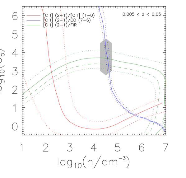
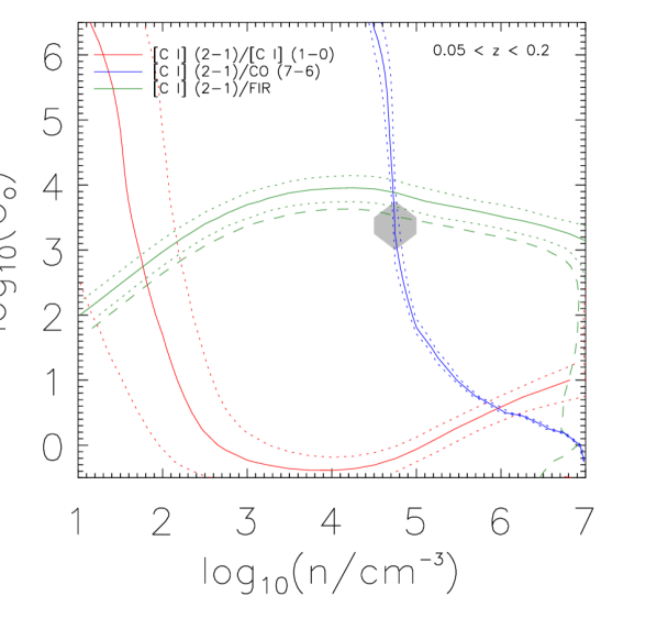
Figure 17.— PDR modeling of observed fluxes in $0.005<z<0.05$ bin (left) and $0.05<z<0.2$ (right). The solid lines are constraint contours determined from modeling, and the dotted lines are the 1$\sigma$ uncertainties. The dashed lines indicate the changes in line flux ratios when the FIR correction (see text) is applied. The gray regions indicate the most likely values of $n$ and $G_{0}$ determined from a likelihood analysis using the corrected flux values of FIR. Table 5 lists the flux values for these two redshift bins before FIR corrections were applied. The line fluxes are in units of $\rm{Wm^{-2}}$, and the L_IR is the far-infrared flux, where the wavelength range that defines L_IR is converted to 30-1000 $\mu$m (Farrah et al., 2013).

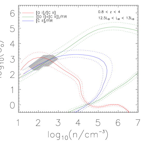
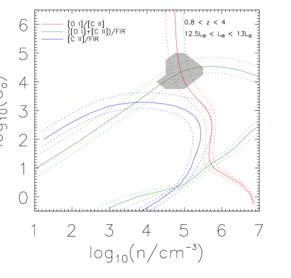
Figure 18.— Left: PDR modeling of observed fluxes for sources with $0.8<z<4$ in the luminosity bin $10^{12.5}\,L_{\odot}<L_{\rm IR}<10^{13}\,L_{\odot}$. No correction factors (see text) are applied to the line and line-FIR ratios in this plot. The gray regions indicates the most likely values of $n$ and $G_{0}$ determined from a likelihood analysis. The uncorrected ratios used for PDR modeling are given in Table 4. The line fluxes are in units of $\rm{Wm^{-2}}$, and the FIR is the far-infrared flux, where the wavelength range that defines L_IR is converted to 30-1000 $\mu$m (Farrah et al., 2013). Though sources in this redshift range are split into three bins based on total infrared luminosity in the text (L${}_{\rm IR}<10^{12.5}\,$L_⊙, $10^{12.5}\,$L${}_{\odot}\,<\,$L${}_{\rm IR}<10^{13}\,$L_⊙, and L${}_{\rm IR}>10^{13}\,$L_⊙), the lack of [O I] detections in the first and third bins mean that PDR models for only the second bin are presented. Right: Same PDR model as on the left but with the correction factors discussed in the text taken into account. The most variation appears in the [O I]/[C II] ratio, which shifts the intersection region from log($n$) $\sim$ 2.5 and log($G_{0}$) $\sim$ 2.5 to log($n$) $\sim$ 5 and log($G_{0}$) $\sim$ 4.

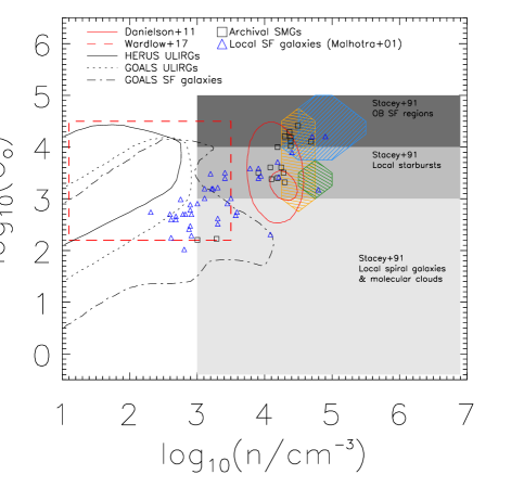
Figure 19.— The results of PDR modeling compared to results from the literature. The light blue region represents the derived n-G₀ for sources with $0.8<z<4$ and $12.5<L/L_{\odot}<13.0$. The orange and green regions represent the derived quantities for $0.005<z<0.05$ and $0.05<z<0.2$ subsamples, respectively. The regions shown here take into the account the correction factors discussed in the text. For comparison, the conditions for local spiral galaxies, molecular clouds, local starbursts, and galactic OB star-forming regions from Stacey et al. (1991) are shown, as well as data points for local star-forming galaxies from Malhotra (2001) and for SMGs come from Wardlow et al. (2017); Sturm et al. (2010); Cox et al. (2011); Danielson et al. (2011); Valtchanov et al. (2011); Alaghband-Zadeh et al. (2013); Huynh et al. (2014), and Rawle et al. (2014).

The gray shaded regions in Figures 17 and 18 represent the most likely values of n and G₀ given the measured line flux ratios. To generate these regions, we perform a likelihood analysis using a method adapted from Ward et al. (2003). The density n and radiation field strength G₀ are taken as free parameters. For measured line ratios $\vec{R}$ with errors $\vec{\sigma}$, we take a Gaussian form for the probability distribution; namely,

$$\mathrm{P(}\vec{\mathrm{R}}\,|\,\mathrm{n,G_{0},}\,\vec{\sigma})=\prod\limits_{i=1}^{\mathrm{N}}\frac{1}{\sqrt{2\pi}\sigma_{i}}\exp{\bigg{\{}-\frac{1}{2}\bigg{[}\frac{\mathrm{R}_{i}-\mathrm{M}_{i}}{\sigma_{i}}\bigg{]}^{2}\bigg{\}}}$$ (7)

where the R_i are the measured line ratios (i.e., [O I]/[C II], [C II]/FIR, etc.), N is the number of independent line ratios, and the M_i are the theoretical line ratio plots from the PDR toolbox. A grid of discrete points in n, G₀-space ranging from $1<$ log${}_{10}($n$)<7$ and $-0.5<\,$log${}_{10}($G${}_{0})\,<\,6.5$ is constructed. To compute the most likely values of n and G₀, we use Bayes’ theorem:

$$\mathrm{P(n,G_{0}}\,|\,\vec{\mathrm{R}},\vec{\sigma})=\frac{\mathrm{P(n,G_{0})\,P(}\vec{\mathrm{R}}\,|\,\mathrm{n,G_{0}},\vec{\sigma})}{\sum\limits_{\mathrm{n,G_{0}}}\,\mathrm{P(n,G_{0})\,P(}\vec{\mathrm{R}}\,|\,\mathrm{n,G_{0}},\vec{\sigma})}$$ (8)

The prior probability density function, P(n,G₀), is set equal to 1 for all points in the grid with G${}_{0}>10^{2}$. Points with G${}_{0}<10^{2}$ are given a prior probability of 0. The reason for this choice of prior stems from the argument that, given the intrinsic luminosities of our sources ($\sim 10^{11.5-13.5}$L_⊙), low values of G₀ (which include, for example, the value of G₀ at the line convergence in the high-$z$ PDR plot at $\rm{log(n/cm^{-3})\sim 4.5}$ and $\rm{log(G_{0})\sim 0.2}$) would correspond to galaxies with sizes on the order of hundreds of kpc or greater (Wardlow et al., 2017). Such sizes are expected to be unphysical, as typical measurements put galaxy sizes with these luminosities at  $0.5-10\,$kpc (see Wardlow et al. 2017 and references therein). P(n, G${}_{0}\,|\,\vec{\rm R},\vec{\sigma})$ gives the probability for each point in the n-G₀ grid that that point represents the actual conditions in the PDR, given the measured flux ratios. The gray regions in Figures 18 and 17 are 68.2% confidence regions. The relative likelihoods of each of the points in the grid are sorted from highest to lowest, and the cumulative sum for each grid point (the likelihood associated with that grid point summed with the likelihoods of the points preceding it in the high-to-low ordering) is computed. Grid points with a cumulative sum less than 0.682 represent the most likely values of density n and UV radiation intensity G₀, given the measured fluxes, with a total combined likelihood of 68.2%. These points constitute the gray regions.

The data constrain the interstellar gas density to be in the range $\rm{log(n/cm^{-3})\sim 4.5-5.5}$ for both low-$z$ and high-$z$, where these values are estimated from the PDR models with correction factors taken into account. The FUV radiation is constrained to be in the range of $\rm{log(G_{0})\sim 3-4}$ and $\rm{log(G_{0})\sim 3-5}$ for low-$z$ and high-$z$, respectively.

The [C I] (2-1)/[C I] (1-0) line ratio is observed to deviate from the region of maximum likelihood on the $\rm G_{0}$-density diagram (Figure 17). The region of maximum likelihood is shaded in gray in the figure. In fact this ratio is very sensitive to the conditions in the ISM, such that a modest change in the radiation strength or density would shift the line towards the expected locus (Danielson et al., 2011). The PDR models also constrain the assumption for the production of [C I] to that of a thin layer on the surface of far-UV heated molecular ISM whereas several studies (Papadopoulos et al., 2004) point to the coexistence of neutral [C I] along CO in the same volume. These assumptions could also result in the deviations observed in the PDR models.

Figure 19 summarizes our main results of the PDR modeling based on the low and high redshift ISM emission lines from the stacked FTS spectra. We compare these measurements with that of local star-forming galaxies (Malhotra, 2001), local starbursts (Stacey et al., 1991) and archival SMGs. We see from Figure 19 that local DSFGs are on average subject to stronger UV radiation than that of local star-forming galaxies and are more consistent with local starbursts. Our measured density and radiation field strengths are further in agreement with results reported in Danielson et al. (2011) for a single DSFG at $z\sim 2$. Given the uncertainty in filling factors and in the fraction of non-PDR [C II] emission, the [O I]/[C II] ratio contour in Figure 18 may shift downward and to the left toward smaller density and radiation field strength where it would be more consistent with the results in Wardlow et al. (2017) for Herschel/PACS stacked spectra of DSFGs.

6. Summary

• We have stacked a diverse sample of Herschel dusty, star-forming galaxies from redshifts $0.005<z<4$ and with total infrared luminosities from from LIRG levels up to luminosities in excess of $10^{13}\,$L_⊙. The sample is heterogeneous, consisting of starbursts, QSOs, and AGN, among other galaxy types. With this large sample, we presented a stacked statistical analysis of the archival spectra in redshift and luminosity bins.

• We present the CO and H₂O spectral line energy distributions for the stacked spectra.

• Radiative transfer modeling with RADEX places constraints on the gas density and temperature based on [C I] (2-1) 370 $\mu$m and [C I] (1-0) 609 $\mu$m measurements.

• We use PDR modeling in conjunction with measured average fluxes to constrain the interstellar gas density to be in the range $\rm{log(n/cm^{-3})\sim 4.5-5.5}$ for stacks at low and high redshifts. The FUV radiation is constrained to be in the range of $\rm{log(G_{0})\sim 3-4}$ and $\rm{log(G_{0})\sim 3-5}$, for low redshifts and high redshifts, respectively. Large uncertainties are present, especially due to effects such as contributions to the [C II] line flux due to non-PDR emission for which we can only estimate the correction factors to the observed line fluxes. Such uncertainties may lead to further discrepancies between the gas conditions at high- and low-redshifts, which may be understood in terms of nuclear starbursts of local DSFGs and luminous and ultra-luminous infrared galaxies compared to $\sim$ 10 kpc-scale massive starbursts of high-$z$ DSFGs.

Figure 20 shows the stack at $0.005<z<0.05$ resulting from an inverse variance weighting scheme. In the main text, an unweighted average is used for this redshift bin. In Figure 20, sources with low signal-to-noise, such as Arp 220, dominate the stack. Notable in this stack are the absorption features, which are present primarily in Arp 220 and survive the stacking process. Tables LABEL:table:obsids and LABEL:table:all_targets enumerate the sources and source properties used in this work.

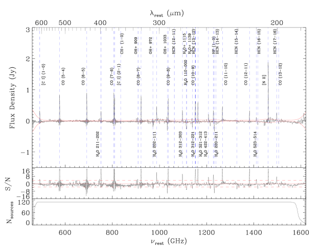
Figure 20.— Top: Stacked SPIRE/FTS spectrum of archival sources with $0.005<z<0.05$ when stacked according to an inverse variance weighting scheme, unlike Figure 3 which is an unweighted mean stack. We present this stack to show how sources such as Arp 220 that were measured with high signal-to-noise can dominate the stack if an inverse variance weighting scheme is used. In particular, strong absorption features from Arp 220 are still identifiable even after stacking. Fluxes from the emission lines in this figure can differ from the fluxes from Figure 3 by as little as 10% or up to a few hundred percent. Large differences in flux are apparent in the H₂O lines, which are significant in the Arp 220 spectrum, but which are reduced in significance when domination of the stack by sources like Arp 220 is removed. Overlaid is the $1\sigma$ jackknifed noise level in red and dashed vertical lines showing the locations of main molecular emission lines. Middle: Signal-to-noise ratio. The horizontal dashed line indicates $\rm S/N=3.5$, and the solid red line indicates $\rm S/N=0$. Lines with $\rm S/N>3.5$ were considered detected. Bottom: The number of sources that contribute to the stack at each wavelength.

Table 6All sources, along with their respective integration times.

Target	Obs. ID	Program	Int. Time [s]
Mrk 231	1342187893	SDP_pvanderw_3	6601
	1342210493	SDP_pvanderw_3	13722
Arp 220	1342190674	KPGT_wilso01_1	9772
IRAS F17207-0014	1342192829	SDP_pvanderw_3	6334
IRAS F18293-3413	1342192830	SDP_pvanderw_3	5279
NGC 1614	1342192831	SDP_pvanderw_3	6334
IRAS F05189-2524	1342192832	SDP_pvanderw_3	16360
	1342192833	SDP_pvanderw_3	16360
IC 4687	1342192993	SDP_pvanderw_3	13986
SDP.81	1342197467	GT1_ivaltcha_1	13194
SDP.130	1342197469	GT1_ivaltcha_1	13194
NGC 7552	1342198428	SDP_pvanderw_3	1717
Arp 299	1342199248	SDP_pvanderw_3	4620
	1342199249	SDP_pvanderw_3	4620
NGC 7469	1342199252	SDP_pvanderw_3	11875
NGC 34	1342199253	SDP_pvanderw_3	14249
NGC 3256	1342201201	SDP_pvanderw_3	4883
ESO 173-G015	1342202268	SDP_pvanderw_3	1717
NGC 1365	1342204020	SDP_pvanderw_3	3168
	1342204021	SDP_pvanderw_3	5279
Mrk 273	1342209850	SDP_pvanderw_3	13062
Arp 193	1342209853	SDP_pvanderw_3	14249
ESO 320-G030	1342210861	SDP_pvanderw_3	5675
IC 1623	1342212314	SDP_pvanderw_3	12799
Mrk 331	1342212316	SDP_pvanderw_3	13061
NGC 7771	1342212317	SDP_pvanderw_3	14249
IRAS 13120-5453	1342212342	SDP_pvanderw_3	3828
NGC 5135	1342212344	SDP_pvanderw_3	14250
CGCG 049-057	1342212346	SDP_pvanderw_3	14250
NGC 6052	1342212347	OT1_nlu_1	2641
MCG +12-02-001	1342213377	SDP_pvanderw_3	1385
MCG-03-04-014	1342213442	OT1_nlu_1	5279
CGCG 436-030	1342213443	OT1_nlu_1	5280
NGC 6240	1342214831	SDP_pvanderw_3	12798
ESO 286-G035	1342216901	OT1_nlu_1	2640
NGC 2623	1342219553	SDP_pvanderw_3	12007
SMMJ2135-0102	1342219562	OT1_rivison_1	13194
GOODS-N07	1342219575	OT1_apope_1	9237
CGCG 448-020	1342221679	OT1_nlu_1	2641
MCG+04-48-002	1342221682	OT1_nlu_1	1321
UGC 12150	1342221699	OT1_nlu_1	2640
IC 5298	1342221700	OT1_nlu_1	2640
NGC 7679	1342221701	OT1_nlu_1	2640
NGC 7592	1342221702	OT1_nlu_1	2641
NGC 0232	1342221707	OT1_nlu_1	2641
ESO 244-G012	1342221708	OT1_nlu_1	2641
NGC 3221	1342221714	OT1_nlu_1	1322
NGC 6286	1342221715	OT1_nlu_1	1322
NGC 6621	1342221716	OT1_nlu_1	2641
IRAS 03158+4227	1342224764	OT1_dfarrah_1	9237
NGC 0695	1342224767	OT1_nlu_1	5279
IRAS 23365+3604	1342224768	OT1_dfarrah_1	5279
IRAS 14378-3651	1342227456	OT1_dfarrah_1	5939
UGC 03094	1342227522	OT1_nlu_1	2641
IRAS 04271+3849	1342227786	OT1_nlu_1	2641
NGC 1961	1342228708	OT1_nlu_1	1321
MCG+02-20-003	1342228728	OT1_nlu_1	2641
NGC 2342	1342228729	OT1_nlu_1	2641
IRAS 05223+1908	1342228738	OT1_nlu_1	2641
UGC 03608	1342228744	OT1_nlu_1	2641
IRAS 05442+1732	1342230413	OT1_nlu_1	1322
MCG+08-11-002	1342230414	OT1_nlu_1	1322
UGC 03351	1342230415	OT1_nlu_1	1322
IRAS F17138-1017	1342230418	OT1_nlu_1	1321
ESO 099-G004	1342230419	OT1_nlu_1	5279
IRAS 06035-7102	1342230420	OT1_dfarrah_1	7258
IRAS 08311-2459	1342230421	OT1_dfarrah_1	7258
IRAS 06206-6315	1342231038	OT1_dfarrah_1	9237
IRAS 19254-6315	1342231039	OT1_dfarrah_1	7258
ESO 069-IG006	1342231040	OT1_nlu_1	7918
NGC 6156	1342231041	OT1_nlu_1	1322
ESO 138-G027	1342231042	OT1_nlu_1	2641
IRAS 17578-0400	1342231047	OT1_nlu_1	1322
IRAS 20087-0308	1342231049	OT1_dfarrah_1	9237
NGC 6926	1342231050	OT1_nlu_1	2640
UGC 11041	1342231061	OT1_nlu_1	2640
IRAS 09022-3615	1342231063	OT1_nlu_1	7917
NGC 4194	1342231069	OT1_nlu_1	1321
NGC 2388	1342231071	OT1_nlu_1	1321
UGC 03410	1342231072	OT1_nlu_1	1321
IRAS 19297-0406	1342231078	OT1_dfarrah_1	5279
NGC 2369	1342231083	OT1_nlu_1	1322
ESO 255-IG007	1342231084	OT1_nlu_1	5279
NGC 3110	1342231971	OT1_nlu_1	1321
IRAS 08355-4944	1342231975	OT1_nlu_1	2641
G09v1.40	1342231977	OT1_rivison_1	13194
IRAS 08572+3915	1342231978	OT1_dfarrah_1	5279
HerMES-Lock01	1342231980	OT2_rivison_2	13195
G09v1.326	1342231985	OT1_rivison_1	13195
SDP.9	1342231986	OT1_rivison_1	13195
G09v1.97	1342231988	OT1_rivison_1	13194
SPT0538-50	1342231989	OT1_dmarrone_1	13194
ESO 339-G011	1342231990	OT1_nlu_1	2640
NGC 6701	1342231994	OT1_nlu_1	1321
NGC 5010	1342236996	OT1_nlu_1	1321
VV 340	1342238241	OT1_nlu_1	5279
UGC 545	1342238246	SDP_pvanderw_3	15042
IRAS 16090-0139	1342238699	OT1_dfarrah_1	10556
G15v2.235	1342238700	OT1_rivison_1	13194
G15v2.19	1342238701	OT1_rivison_1	13194
IRAS 03521+0028	1342238704	OT1_dfarrah_1	11875
HXMM02	1342238706	OT2_rivison_2	13195
Mrk 1014	1342238707	SDP_pvanderw_3	13495
HBootes03	1342238709	OT2_rivison_2	13195
Mrk 478	1342238710	SDP_pvanderw_3	5279
IRAS 15250+3609	1342238711	OT1_dfarrah_1	5279
VV 705	1342238712	OT1_nlu_1	5279
NGC 0958	1342239339	OT1_nlu_1	2641
UGC 02238	1342239340	OT1_nlu_1	2641
UGC 02369	1342239341	OT1_nlu_1	5279
NGC 0877	1342239342	OT1_nlu_1	1322
IRAS F01417+1651	1342239343	OT1_nlu_1	2641
UGC 02608	1342239356	OT1_nlu_1	2641
NGC 0828	1342239357	OT1_nlu_1	1321
NGC 0317B	1342239358	OT1_nlu_1	2641
IC 4734	1342240013	OT1_nlu_1	1322
NGC 5990	1342240016	OT1_nlu_1	1323
UGC 02982	1342240021	OT1_nlu_1	1322
UGC 01845	1342240022	OT1_nlu_1	1322
NGC 1572	1342242588	OT1_nlu_1	2640
MCG-05-12-006	1342242589	OT1_nlu_1	2640
ESO 420-G013	1342242590	OT1_nlu_1	1321
PG 1613+658	1342242593	SDP_pvanderw_3	13194
FLS02	1342242594	OT2_drigopou_3	13194
	1342259071	OT2_drigopou_3	13195
IRAS 20414-1651	1342243623	OT1_dfarrah_1	9237
IRAS 22491-1808	1342245082	OT1_dfarrah_1	7258
IRAS 01003-2238	1342246256	OT1_dfarrah_1	11875
IRAS 20100-4156	1342245106	OT1_dfarrah_1	7258
ESO 286-IG019	1342245107	OT1_nlu_1	5279
ESO 467-G027	1342245108	OT1_nlu_1	2641
IC 5179	1342245109	OT1_nlu_1	1322
ESO 148-IG002	1342245110	OT1_nlu_1	6994
NGC 7674	1342245858	OT1_nlu_1	5279
IRAS 00397-1312	1342246257	OT1_dfarrah_1	13194
IRAS 00188-0856	1342246259	OT1_dfarrah_1	11875
SWIRE05	1342246268	OT2_drigopou_3	13194
IRAS 23230-6926	1342246276	OT1_dfarrah_1	10555
IRAS 23253-5415	1342246277	OT1_dfarrah_1	11875
ESO 350-IG038	1342246978	OT1_nlu_1	2641
DAN03	1342246979	OT2_drigopou_3	13194
IRAS F10565+2448	1342247096	OT1_nlu_1	5279
BOOTES01	1342247113	OT2_drigopou_3	13194
IRAS 10378+1109	1342247118	OT1_dfarrah_1	11875
UGC 08739	1342247123	OT1_nlu_1	2641
NGC 5653	1342247565	OT1_nlu_1	1322
NGC 5104	1342247566	OT1_nlu_1	2641
MCG-02-33-098	1342247567	OT1_nlu_1	2641
ESO 353-G020	1342247615	OT1_nlu_1	2641
MCG-02-01-051	1342247617	OT1_nlu_1	2641
NGC 0023	1342247622	OT1_nlu_1	1322
G12v2.43	1342247744	OT1_rivison_1	13194
G12v2.30	1342247758	OT1_rivison_1	13195
G12v2.257	1342247759	OT1_rivison_1	13195
IRAS 11095-0238	1342247760	OT1_dfarrah_1	10556
IRAS 12071-0444	1342248239	OT1_dfarrah_1	11875
NGP-NC.v1.143	1342248412	OT1_rivison_1	13194
NGP-NA.v1.56	1342248416	OT1_rivison_1	13194
NGC 5734	1342248417	OT1_nlu_1	1321
ESO 507-G070	1342248421	OT1_nlu_1	2641
MCG-03-34-064	1342249041	OT1_nlu_1	2640
IC 4280	1342249042	OT1_nlu_1	2640
ESO 264-G057	1342249043	OT1_nlu_1	2640
ESO 264-G036	1342249044	OT1_nlu_1	2640
IRAS 15462-0450	1342249045	OT1_dfarrah_1	11875
NGC 5936	1342249046	OT1_nlu_1	1321
Mrk 463	1342249047	OT1_dfarrah_1	11875
NGP-NB.v1.78	1342249063	OT1_rivison_1	13194
NGP-NB.v1.43	1342249064	OT1_rivison_1	13194
NGP-NA.v1.144	1342249066	OT1_rivison_1	13195
IRAS 14348-1447	1342249457	OT1_dfarrah_1	5939
ESO 221-IG010	1342249461	OT1_nlu_1	1322
IRAS 12116-5615	1342249462	OT1_nlu_1	5279
IC 4518AB	1342250514	OT1_nlu_1	2641
CGCG 052-037	1342251284	OT1_nlu_1	5279
IRAS F16399-0937	1342251334	OT1_nlu_1	5279
IRAS F16516-0948	1342251335	OT1_nlu_1	5279
SWIRE04	1342253658	OT2_drigopou_3	13194
IRAS 07598+6508	1342253659	OT1_dfarrah_1	11875
MM J18423+5938	1342253672	OT2_maravena_2	15833
	1342255798	OT2_maravena_2	17152
	1342255810	OT2_maravena_2	17152
	1342255811	OT2_maravena_2	17152
	1342255812	OT2_maravena_2	17152
	1342256357	OT2_maravena_2	17152
MG 0751+2716	1342253966	OT1_mbradfor_1	21110
APM 08279+5255	1342253967	OT1_mbradfor_1	21110
SWIRE01	1342254034	OT2_drigopou_3	13194
SWIRE03	1342254035	OT2_drigopou_3	13194
SWIRE02	1342255265	OT2_drigopou_3	13195
SDP.17	1342255280	OT1_rivison_1	13194
SDP.11	1342255281	OT1_rivison_1	13194
G09v1.124	1342255282	OT1_rivison_1	13194
IRAS FSC10214+4724	1342255799	OT1_mbradfor_1	21110
GOODS-N26	1342256083	OT1_apope_1	9236
GOODS-N19	1342256358	OT1_apope_1	9236
GOODS-NC1	1342256359	OT1_apope_1	9236
NGC 7591	1342257346	OT1_nlu_1	2640
BOOTES03	1342257936	OT2_drigopou_3	13195
HXMM01	1342258698	OT2_drigopou_3	13194
FLS01	1342258701	OT2_drigopou_3	13194
BOOTES02	1342259073	OT2_drigopou_3	13195
Cloverleaf	1342259573	OT1_mbradfor_1	21110
CDFS01	1342259582	OT2_drigopou_3	13195
CDFS02	1342259583	OT2_drigopou_3	13194
CDFS04	1342259584	OT2_drigopou_3	13195
SMMJ02399-0136	1342262900	OT2_cferkinh_1	17811

Table 7Properties of sources included in the stacks.

Target	R.A.	DEC.	$z_{spec}$	$\mu$	LIR	Refs.
NGC 7552	23:16:10.80	-42:35:04.65	0.0054	-	11.11	R15,G14,A09
NGC 1365	03:33:36.61	-36:08:18.05	0.00546	-	11.00	R15,A09
NGC 4194	12:14:09.78	+54:31:34.36	0.008342	-	11.10	A09,L17
NGC 3256	10:27:51.18	-43:54:14.21	0.0094	-	11.64	R15,G14,A09
ESO 173-G015	13:27:23.73	-57:29:22.96	0.0097	-	11.38	R15,G14,A09
NGC 5010	13:12:26.52	-15:47:51.75	0.009924	-	11.50	A09,L17
ESO 221-IG010	13:50:56.87	-49:03:18.66	0.010337	-	11.22	A09,L17
Arp 299	11:28:33.31	+58:33:44.89	0.0104	-	11.93	R15,NED,A09
ESO 320-G030	11:53:11.63	-39:07:49.34	0.0108	-	11.17	R15,G14,A09
NGC 2369	07:16:37.96	-62:20:35.71	0.010807	-	11.16	A09,L17
NGC 6156	16:34:52.26	-60:37:06.06	0.010885	-	11.14	A09,L17
IC 5179	22:16:09.08	-36:50:36.54	0.011415	-	11.24	A09,L17
NGC 5653	14:30:09.89	+31:12:56.97	0.011881	-	11.13	A09,L17
ESO 420-G013	04:13:49.69	-32:00:24.34	0.011908	-	11.07	A09,L17
NGC 5990	15:46:16.41	+02:24:54.68	0.012806	-	11.13	A09,L17
CGCG 049-057	15:13:13.18	+07:13:30.24	0.013	-	11.35	R15,A09
NGC 0877	02:18:00.12	+14:32:34.34	0.013052	-	11.10	A09,L17
UGC 03410	06:14:30.27	+80:27:00.89	0.013079	-	11.10	A09,L17
NGC 1961	05:42:04.67	+69:22:42.69	0.013122	-	11.06	A09,L17
NGC 6701	18:43:12.47	+60:39:09.42	0.013226	-	11.12	A09,L17
NGC 5936	15:30:00.76	+12:59:20.78	0.013356	-	11.14	A09,L17
NGC 5135	13:25:44.09	-29:49:59.51	0.0137	-	11.30	R15,G14,A09
NGC 3221	10:22:20.36	+21:34:21.41	0.013709	-	11.09	A09,L17
NGC 5734	14:45:09.02	-20:52:13.17	0.013746	-	11.15	A09,L17
NGC 2388	07:28:53.51	+33:49:08.56	0.01379	-	11.28	A09,L17
MCG+04-48-002	20:28:35.15	+25:44:03.27	0.0139	-	11.11	A09,L17
IRAS 17578-0400	18:00:31.78	-04:00:54.86	0.014043	-	11.48	A09,L17
NGC 7771	23:51:24.67	+20:06:40.24	0.0143	-	11.40	R15,G14,A09
UGC 03351	05:45:48.22	+58:42:05.69	0.01486	-	11.28	A09,L17
NGC 0023	00:09:53.39	+25:55:25.98	0.015231	-	11.12	A09,L17
UGC 01845	02:24:07.87	+47:58:11.61	0.015607	-	11.12	A09,L17
IC 4734	18:38:25.65	-57:29:25.01	0.015611	-	11.35	A09,L17
MCG+12-02-001	00:54:03.47	+73:05:10.14	0.0157	-	11.50	R15,G14,A09
IC 4518AB	14:57:41.12	-43:07:56.00	0.015728	-	11.23	A09,L17
NGC 6052	16:05:12.93	+20:32:36.42	0.015808	-	11.09	A09,L17
NGC 1614	04:33:59.75	-08:34:44.84	0.0159	-	11.65	R15,G14,A09
ESO 353-G020	01:34:51.30	-36:08:14.57	0.015921	-	11.06	A09,L17
MCG-02-33-098	13:02:19.78	-15:46:03.69	0.015921	-	11.17	A09,L17
MCG+02-20-003	07:35:43.63	+11:42:36.02	0.016255	-	11.13	A09,L17
UGC 11041	17:54:51.76	+34:46:32.76	0.016281	-	11.11	A09,L17
NGC 7469	23:03:15.79	+08:52:28.62	0.0163	-	11.65	R15,G14,A09
IC 4280	13:32:53.31	-24:12:25.81	0.016331	-	11.15	A09,L17
NGC 7591	23:18:16.34	+06:35:09.43	0.016531	-	11.12	A09,L17
MCG-03-34-064	13:22:24.43	-16:43:42.76	0.016541	-	11.28	A09,L17
UGC 08739	13:49:14.26	+35:15:19.63	0.016785	-	11.15	A09,L17
NGC 3110	10:04:02.20	-06:28:28.08	0.016858	-	11.37	A09,L17
NGC 7679	23:28:46.63	+03:30:43.34	0.017139	-	11.11	A09,L17
ESO 264-G057	10:59:01.79	-43:26:25.61	0.017199	-	11.14	A09,L17
IC 4687	18:13:39.82	-57:43:30.54	0.0173	-	11.62	R15,G14,A09
IRAS F17138-1017	17:16:35.74	-10:20:41.31	0.017335	-	11.49	A09,L17
ESO 286-G035	21:04:11.06	-43:35:30.24	0.017361	-	11.20	A09,L17
ESO 467-G027	22:14:39.81	-27:27:50.32	0.017401	-	11.08	A09,L17
NGC 2342	07:09:18.22	+20:38:11.26	0.017599	-	11.31	A09,L17
UGC 02982	04:12:22.51	+05:32:49.65	0.017696	-	11.20	A09,L17
NGC 0828	02:10:09.45	+39:11:25.50	0.017926	-	11.36	A09,L17
Arp 220	15:34:57.22	+23:30:12.34	0.0181	-	12.28	R11,R15,A09
NGC 0317B	00:57:40.32	+43:47:31.94	0.018109	-	11.19	A09,L17
IRAS F18293-3413	18:32:41.36	-34:11:25.88	0.0182	-	11.88	R15,A09
NGC 6286	16:58:31.38	+58:56:15.38	0.018349	-	11.37	A09,L17
NGC 2623	08:38:24.06	+25:45:17.00	0.0185	-	11.60	R15,G14,A09
Mrk 331	23:51:26.53	+20:35:09.12	0.0185	-	11.50	R15,G14,A09
NGC 5104	13:21:22.99	+00:20:33.32	0.018606	-	11.27	A09,L17
IRAS 05442+1732	05:47:11.24	+17:33:47.37	0.01862	-	11.30	A09,L17
MCG-05-12-006	04:52:04.97	-32:59:25.66	0.018753	-	11.17	A09,L17
IRAS 04271+3849	04:30:33.23	+38:55:48.62	0.018813	-	11.11	A09,L17
NGC 0958	02:30:42.79	-02:56:23.96	0.01914	-	11.20	A09,L17
MCG+08-11-002	05:40:43.73	+49:41:41.58	0.019157	-	11.46	A09,L17
ESO 339-G011	19:57:37.37	-37:56:08.47	0.0192	-	11.20	A09,L17
NGC 34	00:11:06.54	-12:06:23.70	0.0196	-	11.49	R15,G14,A09
NGC 6926	20:33:06.02	-02:01:40.02	0.019613	-	11.32	A09,L17
IC 1623	01:07:46.72	-17:30:27.31	0.0201	-	11.71	R15,G14,A09
NGC 1572	04:22:42.75	-40:36:03.31	0.020384	-	11.30	A09,L17
ESO 350-IG038	00:36:52.39	-33:33:17.36	0.020598	-	11.28	A09,L17
NGC 6621	18:12:55.21	+68:21:46.48	0.020652	-	11.29	A09,L17
ESO 138-G027	17:26:43.00	-59:55:54.34	0.020781	-	11.41	A09,L17
ESO 264-G036	10:43:07.67	-46:12:44.83	0.021065	-	11.32	A09,L17
UGC 03608	06:57:34.59	+46:24:11.62	0.021351	-	11.34	A09,L17
UGC 12150	22:41:12.20	+34:14:53.38	0.021391	-	11.35	A09,L17
ESO 507-G070	13:02:52.32	-23:55:17.90	0.021702	-	11.56	A09,L17
UGC 02238	02:46:17.42	+13:05:45.17	0.021883	-	11.33	A09,L17
NGC 0232	00:42:45.76	-23:33:39.06	0.022639	-	11.44	A09,L17
IRAS F16516-0948	16:54:23.78	-09:53:21.05	0.022706	-	11.32	A09,L17
ESO 244-G012	01:18:08.31	-44:27:38.75	0.022903	-	11.38	A09,L17
Arp 193	13:20:35.49	+34:08:22.52	0.0233	-	11.73	R15,G14,A09
UGC 02608	03:15:01.23	+42:02:08.76	0.023343	-	11.41	A09,L17
NGC 7592	23:18:22.22	-04:24:56.56	0.024444	-	11.40	A09,L17
UGC 03094	04:35:33.85	+19:10:18.51	0.02471	-	11.44	A09,L17
CGCG 052-037	16:30:56.58	+04:04:58.99	0.02449	-	11.45	A09,L17
NGC 6240	16:52:59.10	+02:24:04.07	0.0245	-	11.93	R15,G14,A09
IRAS 08355-4944	08:37:02.00	-49:54:29.02	0.025898	-	11.62	A09,L17
IRAS F16399-0937	16:42:40.11	-09:43:13.41	0.027012	-	11.63	A09,L17
IRAS 12116-5615	12:14:22.18	-56:32:32.78	0.027102	-	11.65	A09,L17
MCG-02-01-051	00:18:50.85	-10:22:37.73	0.027299	-	11.48	A09,L17
IRAS F01417+1651	01:44:30.50	+17:06:08.40	0.027399	-	11.64	A09,L17
IC 5298	23:16:00.62	+25:33:22.03	0.027422	-	11.60	A09,L17
NGC 7674	23:27:56.74	+08:46:43.49	0.028924	-	11.56	A09,L17
ESO 099-G004	15:24:57.73	-63:07:30.44	0.029284	-	11.74	A09,L17
IRAS 05223+1908	05:25:16.75	+19:10:49.25	0.029577	-	11.65	A09,L17
IRAS 13120-5453	13:15:06.42	-55:09:21.22	0.0308	-	12.34	R15,G14
UGC 02369	02:54:01.75	+14:58:13.49	0.031202	-	11.67	A09,L17
CGCG 436-030	01:20:02.47	+14:21:40.61	0.031229	-	11.69	A09,L17
NGC 0695	01:51:14.37	+22:34:55.81	0.032472	-	11.68	A09,L17
VV 340	14:57:00.78	+24:37:04.37	0.033669	-	11.74	A09,L17
MCG-03-04-014	01:10:08.85	-16:51:11.29	0.035144	-	11.65	A09,L17
CGCG 448-020	20:57:24.32	+17:07:37.28	0.036098	-	11.94	A09,L17
Mrk 273	13:44:42.42	+55:53:11.78	0.0378	-	12.21	R15,G14,A09
ESO 255-IG007	06:27:21.68	-47:10:36.83	0.03879	-	11.90	A09,L17
VV 705	15:18:06.26	+42:44:43.68	0.040191	-	11.92	A09,L17
Mrk 231	12:56:14.46	+56:52:24.92	0.0422	-	12.57	R15,G14,A09,V10
IRAS F05189-2524	05:21:01.29	-25:21:45.21	0.0426	-	12.16	R15,G14,A09
IRAS F17207-0014	17:23:21.98	-00:17:00.96	0.0428	-	12.46	R15,A09
ESO 286-IG019	20:58:26.81	-42:38:59.71	0.042996	-	12.06	A09,L17
IRAS F10565+2448	10:59:18.17	+24:32:34.26	0.0431	-	12.08	A09,L17
ESO 148-IG002	23:15:46.70	-59:03:14.91	0.044601	-	12.06	A09,L17
ESO 069-IG006	16:38:11.46	-68:26:07.94	0.046972	-	11.98	A09,L17
Mrk 463	13:56:02.86	+18:22:20.05	0.051	-	11.79	M90,F07,F13
IRAS 15250+3609	15:26:59.56	+35:58:37.63	0.055	-	12.00	M90,F07,I11
IRAS 08572+3915	09:00:25.70	+39:03:54.83	0.058	-	12.11	M90,F07,G14
UGC 545	00:53:34.86	+12:41:34.87	0.0589	-	11.93	S11,E06,NED
IRAS 09022-3615	09:04:12.87	-36:27:00.14	0.059641	-	12.31	A09,L17
IRAS 19254-6315	19:31:20.23	-72:39:22.89	0.063	-	12.09	M90,F07,F13
IRAS 23365+3604	23:39:01.08	+36:21:09.28	0.064	-	12.15	M90,F07,G14
IRAS 14378-3651	14:40:58.89	-37:04:32.47	0.068	-	12.23	HW88,F07,I11
IRAS 22491-1808	22:51:49.20	-17:52:23.62	0.078	-	11.65	M90,F07,F13
IRAS 06035-7102	06:02:54.36	-71:03:08.81	0.079	-	12.22	M90,F07 ,F13
Mrk 478	14:42:07.61	+35:26:23.22	0.0791	-	11.52	E06,S11,NED
IRAS 14348-1447	14:37:38.29	-15:00:24.75	0.083	-	12.42	HW88,F07,G14
IRAS 19297-0406	19:32:21.84	-04:00:02.83	0.086	-	12.45	HW88,F07,I11
IRAS 20414-1651	20:44:18.25	-16:40:16.02	0.087	-	12.22	HW88,F07,F13
IRAS 06206-6315	06:21:01.47	-63:17:23.12	0.092	-	12.23	M90,F07,F13
IRAS 08311-2459	08:33:20.65	-25:09:32.20	0.100	-	12.50	HW88,F07 ,F13
IRAS 15462-0450	15:48:56.83	-04:59:33.71	0.100	-	12.24	M90,F07,F13
IRAS 20087-0308	20:11:23.73	-02:59:50.82	0.106	-	12.42	HW88,F07,F13
IRAS 11095-0238	11:12:03.35	-02:54:23.93	0.107	-	12.28	HW88,F07,F13
IRAS 23230-6926	23:26:03.52	-69:10:19.11	0.107	-	12.37	M90,F07,F13
IRAS 01003-2238	01:02:49.92	-22:21:56.47	0.118	-	12.32	HW88,F07,F13
IRAS 00188-0856	00:21:26.52	-08:39:26.86	0.128	-	12.39	M90,F07 ,F13
IRAS 12071-0444	12:09:45.13	-05:01:13.46	0.128	-	12.41	M90,F07,F13
PG 1613+658	16:13:57.15	+65:43:09.19	0.129	-	11.88	NED,E06
IRAS 20100-4156	20:13:29.68	-41:47:34.68	0.13	-	12.67	HW88,F07,F13
IRAS 23253-5415	23:28:06.15	-53:58:30.96	0.13	-	12.36	M90,F07,F13
IRAS 03158+4227	03:19:12.50	+42:38:28.37	0.134	-	12.63	HW88,F07,F13
IRAS 16090-0139	16:11:40.61	-01:47:05.86	0.134	-	12.55	M90,F07,F13
IRAS 10378+1109	10:40:29.13	+10:53:18.36	0.136	-	12.31	HW88,F07,F13
SWIRE03	10:40:43.66	+59:34:09.66	0.148	-	12.25	M90,H03,Y13
IRAS 07598+6508	08:04:30.36	+64:59:52.76	0.148	-	12.50	M90,F07,F13
IRAS 03521+0028	03:54:42.10	+00:37:00.71	0.152	-	12.52	HW88,F07 ,F13
Mrk 1014	01:59:50.10	+00:23:39.10	0.1631	-	12.62	F13,NED
CDFS04	03:35:49.16	-27:49:18.29	0.168	-	11.80	E09,D09,M90,M11
BOOTES03	14:28:49.80	+34:32:39.81	0.219	-	11.87	M14
CDFS02	03:28:18.03	-27:43:08.25	0.248	-	11.82	M14
BOOTES02	14:32:34.88	+33:28:32.25	0.25	-	11.91	M14
SWIRE04	10:32:37.47	+58:08:45.75	0.251	-	11.80	M14
IRAS 00397-1312	00:42:15.50	-12:56:03.17	0.262	-	12.90	HW88,F07
DAN03	00:40:14.68	-43:20:10.81	0.265	-	11.59	M14
CDFS01	03:29:04.38	-28:47:52.52	0.289	-	11.79	M14
BOOTES01	14:36:31.97	+34:38:29.60	0.354	-	12.69	M14
SWIRE02	10:51:13.42	+57:14:25.79	0.362	-	11.90	M14
SWIRE05	10:35:58.01	+58:58:46.17	0.366	-	12.06	M14
FLS01	17:20:17.08	+59:16:37.47	0.417	-	11.86	M14
FLS02	17:13:31.69	+58:58:04.60	0.436	-	12.41	M14
SWIRE01	10:47:53.34	+58:21:05.99	0.887	-	12.92	M14
G15v2.19*	14:29:35.27	-00:28:36.23	1.027	9.7 $\pm$ 0.7	12.42	ME14,W17
GOODS-N26	12:36:34.53	+62:12:39.74	1.219	-	12.26	G14,M12
HBootes03	14:28:24.16	+35:26:19.84	1.326	3.0 $\pm$ 1.5	12.69	B13
SDP.9	09:07:40.22	-00:41:59.03	1.577	8.8 $\pm$ 2.2	12.58	B13
NGP-NB.v1.43	13:24:27.23	+28:44:50.37	1.68	2.8 $\pm$ 0.4	12.92	B13,T16
SDP.11	09:10:43.04	-00:03:22.72	1.784	10.9 $\pm$ 1.3	12.48	B13
GOODS-N07	12:36:21.22	+62:17:10.32	1.9924	-	12.42	M12
GOODS-NC1	12:36:00.25	+62:10:47.13	2.0017	-	12.22	G14
G09v1.40*	08:53:59.04	+01:55:38.05	2.0894	15.3 $\pm$ 3.5	12.45	B13,W17
G12v2.257*	11:58:20.06	-01:37:52.10	2.191	13.0 $\pm$ 7.0	12.04	W17
NGP-NA.v1.144*	13:36:49.88	+29:18:00.95	2.202	4.4 $\pm$ 0.8	12.95	B13,W17
IRAS FSC10214+4724	10:24:34.58	+47:09:10.11	2.286	50	12.46	BL95,RR93,B99
NGP-NA.v1.56*	13:44:29.41	+30:30:36.10	2.301	11.7 $\pm$ 0.9	12.77	B13,W17
SDP.17	09:03:02.83	-01:41:25.84	2.3051	4.9 $\pm$ 0.7	13.00	B13
HXMM01*	02:20:16.53	-06:01:43.67	2.308	1.5 $\pm$ 0.3	13.30	B13,W17
SMMJ2135-0102	21:35:11.60	-01:02:52.16	2.326	37.5 $\pm$ 4.5	12.41	I10b,SW11
G09v1.124*	08:49:33.31	+02:14:42.61	2.410	2.8 $\pm$ 0.2	13.14	B13,W17
G15v2.235*	14:13:52.18	-00:00:23.84	2.478	1.8 $\pm$ 0.3	13.26	B13,W17
GOODS-N19	12:37:07.26	+62:14:07.55	2.484	-	12.57	M12
Cloverleaf	14:15:46.26	+11:29:43.45	2.56	11	12.78	B92,B99,VS03,U16
G09v1.326*	09:18:40.85	+02:30:47.37	2.581	-	12.76	B13,W17
SDP.130	09:13:05.30	-00:53:42.80	2.626	2.1 $\pm$ 0.3	13.30	B13
SMMJ02399-0136	02:39:51.89	-01:35:58.56	2.795	2.38 $\pm$ 0.08	12.73	G14,I10a,T12
SPT0538-50	05:38:16.77	-50:30:53.66	2.782	21 $\pm$ 4	12.54	BW13
HerMES-Lock01	10:57:51.21	+57:30:27.83	2.956	9.2 $\pm$ 0.4	13.06	B13
SDP.81	09:03:11.50	+00:39:06.70	3.043	11.1 $\pm$ 1.1	12.57	B13
NGP-NB.v1.78*	13:30:08.34	+24:59:00.07	3.111	13.0 $\pm$ 1.5	12.78	B13,W17
G12v2.43*	11:35:26.16	-01:46:06.84	3.127	2.8 $\pm$ 0.4	12.70	B13,W17
MG 0751+2716	07:51:41.62	+27:16:32.67	3.2	16	11.77	A07,BI02,B02,WU09
G12v2.30*	11:46:37.96	-00:11:32.89	3.259	9.5 $\pm$ 0.6	13.06	B13,W17
HXMM02	02:18:30.56	-05:31:31.85	3.39	4.4 $\pm$ 1.0	12.90	B13
NGP-NC.v1.143	12:56:32.65	+23:36:25.55	3.565	11.3 $\pm$ 1.7	12.91	B13
G09v1.97	08:30:51.12	+01:32:26.00	3.634	6.9 $\pm$ 0.6	13.20	B13
APM 08279+5255	08:31:41.59	+52:45:17.81	3.91	4	13.78	E00,R09,B06,K07,LI11,V11
MM J18423+5938	18:42:22.50	+59:38:29.81	3.926	12	12.13	L11,D12
Unused Spectra
HATLAS 090302-014226†	09:03:02.95	-01:42:26.30
SF.V1.88†	23:26:23.03	-34:26:40.34
SF.V1.100†	01:24:07.35	-28:14:35.78
SG.V1.22†	01:37:19.98	-33:19:49.54
SG.V1.29†	01:40:31.14	-32:42:03.51
SG.V1.77†	01:48:34.68	-30:35:32.05
SA.V1.44†	22:38:29.06	-30:41:48.86
SC.V1.128†	23:24:19.84	-32:39:23.71
SD.V1.70†	00:09:12.62	-30:08:09.16
SD.V1.133†	00:07:22.37	-35:20:15.57
SB.V1.143†	23:25:55.44	-30:22:34.89
SGP-B-202†	23:26:23.03	-34:26:40.34
SGP-D-328†	00:26:25.11	-34:17:38.13
SGP-E-165†	00:47:36.05	-27:29:54.03
SGP-A-53†	22:25:36.37	-29:56:46.03
MACS J2043-2144‡	20:43:14.17	-21:44:38.80
MMJ0107†	01:07:02.35	-73:01:59.80
SWIRE 07†	11:02:05.80	+57:57:40.75
XMM 02†	02:19:57.26	-05:23:48.81
DAN 02†	17:20:17.08	+53:12:43.41
Locke 01†	10:45:30.42	+58:12:32.86
HeLMS 44†	23:32:55.44	-03:11:34.34
HeLMS 45†	23:24:39.55	-04:39:36.18
SPT 0551-50††	05:51:39.41	-50:58:02.36	3.164
SPT 0512-59††	05:12:57.93	-59:35:41.87	2.2331
NGC 2146‡‡	06:18:38.91	+78:21:25.37	0.00298
NGC 1068‡‡	02:42:40.82	-00:00:47:56	0.00379
NGC 4151‡‡	12:10:32.88	+39:24:18.55	0.00332
NGC 5128‡‡	13:25:27.55	-43:01:09.79	0.00183
M81‡‡	09:55:32.78	+69:03:57.05	-0.000113
M82‡‡	09:55:51.67	+69:40:48.20	0.000677
NGC 2403‡‡	07:36:49.82	+65:36:12.27	0.000445
NGC 205‡‡	00:40:24.03	+41:41:50.39	-0.000768
MCG 604†	01:34:33.46	+30:46:47.59

Notes: L_IR values for sources with $z<1$ are taken from the literature. The given values of L_IR for sources with $z>1$ are computed from fits to continuum photometry and are corrected for lensing magnification. Sources marked with * have PACS spectroscopy and appear in Wardlow et al. (2017). References: A07: Alloin et al. (2007), A09: Armus et al. (2009), B92: Barvainis et al. (1992), B99: Benford (1999), B02: Barvainis et al. (2002), B06: Beelen et al. (2006), B13: Bussmann et al. (2013), BI02: Barvainis & Ivison (2002), BL95: Broadhurst & Lehar (1995), BW13: Bothwell et al. (2013), D09: Dye et al. (2009), D12: Decarli et al. (2012), E00: Egami et al. (2000), E06: Evans et al. (2006), E09: Eales et al. (2009), F07: Farrah et al. (2007), F13: Farrah et al. (2013), G14: Greve et al. (2014), H03: Hutchings et al. (2003), HW88: Helou & Walker (1988), I10a Ivison et al. (2010a), I10b:Ivison et al. (2010b), V10:van der Werf et al. (2010), I11: Iwasawa et al. (2011), K07: Krips et al. (2007), L11: Lestrade et al. (2011), L17:Lu et al. (2017), LI11: Lis et al. (2011), M90: Moshir & et al. (1990), M11: Moncelsi et al. (2011), M12: Magnelli et al. (2012), M14: Magdis et al. (2014), ME14: Messias et al. (2014), NED: NASA/IPAC Extragalactic Database, R09: Riechers et al. (2009), R11: Rangwala et al. (2011), R15: Rosenberg et al. (2015), RR93: Rowan-Robinson et al. (1993), S11: Sargsyan et al. (2011), S14: Spilker et al. (2014), SW11: Swinbank et al. (2011), T12: Thomson et al. (2012), T16: Timmons et al. (2016), U16: Uzgil et al. (2016), V11: van der Werf et al. (2011), VS03 Venturini & Solomon (2003), W17: Wardlow et al. (2017), WU09: Wu et al. (2009), Y13: Yamada et al. (2013). For unused spectra: ^†No spectroscopic redshift and/or magnification factor. ^‡ Multiple objects within beam. ^†† No magnification factor. ^‡‡Redshift less than 0.005.

References

- Abel (2006) Abel, N. P. 2006, MNRAS, 368, 1949
- Alaghband-Zadeh et al. (2013) Alaghband-Zadeh, S., Chapman, S. C., Swinbank, A. M., et al. 2013, MNRAS, 435, 1493
- Alloin et al. (2007) Alloin, D., Kneib, J.-P., Guilloteau, S., & Bremer, M. 2007, A&A, 470, 53
- Aravena et al. (2016) Aravena, M., Decarli, R., Walter, F., et al. 2016, ApJ, 833, 71
- Armus et al. (2009) Armus, L., Mazzarella, J. M., Evans, A. S., et al. 2009, PASP, 121, 559
- Bakes & Tielens (1994) Bakes, E. L. O., & Tielens, A. G. G. M. 1994, ApJ, 427, 822
- Barvainis et al. (2002) Barvainis, R., Alloin, D., & Bremer, M. 2002, A&A, 385, 399
- Barvainis et al. (1992) Barvainis, R., Antonucci, R., & Coleman, P. 1992, ApJ, 399, L19
- Barvainis & Ivison (2002) Barvainis, R., & Ivison, R. 2002, ApJ, 571, 712
- Beelen et al. (2006) Beelen, A., Cox, P., Benford, D. J., et al. 2006, ApJ, 642, 694
- Benford (1999) Benford, D. J. 1999, PhD thesis, CALIFORNIA INSTITUTE OF TECHNOLOGY
- Bonato et al. (2014) Bonato, M., Negrello, M., Cai, Z.-Y., et al. 2014, MNRAS, 438, 2547
- Bothwell et al. (2013) Bothwell, M. S., Aguirre, J. E., Chapman, S. C., et al. 2013, ApJ, 779, 67
- Bradford et al. (2011) Bradford, C. M., Bolatto, A. D., Maloney, P. R., et al. 2011, ApJ, 741, L37
- Brauher et al. (2008) Brauher, J. R., Dale, D. A., & Helou, G. 2008, ApJS, 178, 280
- Brisbin et al. (2015) Brisbin, D., Ferkinhoff, C., Nikola, T., et al. 2015, ApJ, 799, 13
- Broadhurst & Lehar (1995) Broadhurst, T., & Lehar, J. 1995, ApJ, 450, L41
- Bussmann et al. (2013) Bussmann, R. S., Pérez-Fournon, I., Amber, S., et al. 2013, ApJ, 779, 25
- Calanog et al. (2014) Calanog, J. A., Fu, H., Cooray, A., et al. 2014, ApJ, 797, 138
- Carilli & Walter (2013) Carilli, C. L., & Walter, F. 2013, ARA&A, 51, 105
- Casey (2012) Casey, C. M. 2012, MNRAS, 425, 3094
- Casey et al. (2014) Casey, C. M., Narayanan, D., & Cooray, A. 2014, Phys. Rep., 541, 45
- Chary & Elbaz (2001) Chary, R., & Elbaz, D. 2001, ApJ, 556, 562
- Contursi et al. (2013) Contursi, A., Poglitsch, A., Grácia Carpio, J., et al. 2013, A&A, 549, A118
- Cormier et al. (2015) Cormier, D., Madden, S. C., Lebouteiller, V., et al. 2015, A&A, 578, A53
- Cox et al. (2011) Cox, P., Krips, M., Neri, R., et al. 2011, ApJ, 740, 63
- Danielson et al. (2011) Danielson, A. L. R., Swinbank, A. M., Smail, I., et al. 2011, MNRAS, 410, 1687
- De Looze et al. (2017) De Looze, I., Baes, M., Cormier, D., et al. 2017, Monthly Notices of the Royal Astronomical Society, 465, 3741
- Decarli et al. (2012) Decarli, R., Walter, F., Neri, R., et al. 2012, ApJ, 752, 2
- Díaz-Santos et al. (2013) Díaz-Santos, T., Armus, L., Charmandaris, V., et al. 2013, ApJ, 774, 68
- Dye et al. (2009) Dye, S., Ade, P. A. R., Bock, J. J., et al. 2009, ApJ, 703, 285
- Eales et al. (2009) Eales, S., Chapin, E. L., Devlin, M. J., et al. 2009, ApJ, 707, 1779
- Eales et al. (2010) Eales, S. A., Smith, M. W. L., Wilson, C. D., et al. 2010, A&A, 518, L62
- Egami et al. (2000) Egami, E., Neugebauer, G., Soifer, B. T., et al. 2000, ApJ, 535, 561
- Elbaz et al. (2011) Elbaz, D., Dickinson, M., Hwang, H. S., et al. 2011, A&A, 533, A119
- Evans et al. (2006) Evans, A. S., Solomon, P. M., Tacconi, L. J., Vavilkin, T., & Downes, D. 2006, AJ, 132, 2398
- Farrah et al. (2007) Farrah, D., Bernard-Salas, J., Spoon, H. W. W., et al. 2007, ApJ, 667, 149
- Farrah et al. (2013) Farrah, D., Lebouteiller, V., Spoon, H. W. W., et al. 2013, ApJ, 776, 38
- Ferkinhoff et al. (2014) Ferkinhoff, C., Brisbin, D., Parshley, S., et al. 2014, ApJ, 780, 142
- Fernández-Ontiveros et al. (2016) Fernández-Ontiveros, J. A., Spinoglio, L., Pereira-Santaella, M., et al. 2016, ApJS, 226, 19
- Fischer et al. (1999) Fischer, J., Luhman, M. L., Satyapal, S., et al. 1999, Ap&SS, 266, 91
- Flower & Pineau Des Forêts (2010) Flower, D. R., & Pineau Des Forêts, G. 2010, MNRAS, 406, 1745
- Fulton et al. (2016) Fulton, T., Naylor, D. A., Polehampton, E. T., et al. 2016, MNRAS, 458, 1977
- George (2015) George, R. D. 2015, PhD thesis, University of Edinburgh
- George et al. (2013) George, R. D., Ivison, R. J., Hopwood, R., et al. 2013, MNRAS, 436, L99
- González-Alfonso et al. (2010a) González-Alfonso, E., Fischer, J., Isaak, K., et al. 2010a, A&A, 518, L43
- González-Alfonso et al. (2010b) —. 2010b, A&A, 518, L43
- Greve et al. (2014) Greve, T. R., Leonidaki, I., Xilouris, E. M., et al. 2014, ApJ, 794, 142
- Griffin et al. (2010) Griffin, M. J., Abergel, A., Abreu, A., et al. 2010, A&A, 518, L3
- Gruppioni et al. (2016) Gruppioni, C., Berta, S., Spinoglio, L., et al. 2016, MNRAS, 458, 4297
- Gullberg et al. (2015) Gullberg, B., De Breuck, C., Vieira, J. D., et al. 2015, MNRAS, 449, 2883
- Helou & Walker (1988) Helou, G., & Walker, D. W., eds. 1988, Infrared astronomical satellite (IRAS) catalogs and atlases. Volume 7: The small scale structure catalog, Vol. 7, 1–265
- Hemmati et al. (2017) Hemmati, S., Yan, L., Diaz-Santos, T., et al. 2017, ApJ, 834, 36
- Herrera-Camus et al. (2015) Herrera-Camus, R., Bolatto, A. D., Wolfire, M. G., et al. 2015, ApJ, 800, 1
- Herrera-Camus et al. (2016) Herrera-Camus, R., Bolatto, A., Smith, J. D., et al. 2016, ApJ, 826, 175
- Hezaveh et al. (2013) Hezaveh, Y. D., Marrone, D. P., Fassnacht, C. D., et al. 2013, ApJ, 767, 132
- Hollenbach & Tielens (1997) Hollenbach, D. J., & Tielens, A. G. G. M. 1997, ARA&A, 35, 179
- Hollenbach & Tielens (1999) —. 1999, Reviews of Modern Physics, 71, 173
- Hopkins et al. (2012) Hopkins, P. F., Quataert, E., & Murray, N. 2012, MNRAS, 421, 3488
- Hughes et al. (2016) Hughes, T. M., Baes, M., Schirm, M. R. P., et al. 2016, A&A, 587, A45
- Hutchings et al. (2003) Hutchings, J. B., Maddox, N., Cutri, R. M., & Nelson, B. O. 2003, AJ, 126, 63
- Huynh et al. (2014) Huynh, M. T., Kimball, A. E., Norris, R. P., et al. 2014, MNRAS, 443, L54
- Ivison et al. (2010a) Ivison, R. J., Smail, I., Papadopoulos, P. P., et al. 2010a, MNRAS, 404, 198
- Ivison et al. (2010b) Ivison, R. J., Swinbank, A. M., Swinyard, B., et al. 2010b, A&A, 518, L35
- Iwasawa et al. (2011) Iwasawa, K., Sanders, D. B., Teng, S. H., et al. 2011, A&A, 529, A106
- Kamenetzky et al. (2016) Kamenetzky, J., Rangwala, N., Glenn, J., Maloney, P. R., & Conley, A. 2016, ApJ, 829, 93
- Kaufman et al. (2006) Kaufman, M. J., Wolfire, M. G., & Hollenbach, D. J. 2006, ApJ, 644, 283
- Kaufman et al. (1999) Kaufman, M. J., Wolfire, M. G., Hollenbach, D. J., & Luhman, M. L. 1999, ApJ, 527, 795
- Kennicutt & Evans (2012) Kennicutt, R. C., & Evans, N. J. 2012, ARA&A, 50, 531
- Kennicutt (1998) Kennicutt, Jr., R. C. 1998, ARA&A, 36, 189
- Kirkpatrick et al. (2012) Kirkpatrick, A., Pope, A., Alexander, D. M., et al. 2012, ApJ, 759, 139
- Krips et al. (2007) Krips, M., Peck, A. B., Sakamoto, K., et al. 2007, The Astrophysical Journal Letters, 671, L5
- Lepp & Dalgarno (1988) Lepp, S., & Dalgarno, A. 1988, ApJ, 335, 769
- Leroy et al. (2008) Leroy, A. K., Walter, F., Brinks, E., et al. 2008, AJ, 136, 2782
- Lestrade et al. (2011) Lestrade, J.-F., Carilli, C. L., Thanjavur, K., et al. 2011, ApJ, 739, L30
- Lis et al. (2011) Lis, D. C., Neufeld, D. A., Phillips, T. G., Gerin, M., & Neri, R. 2011, ApJ, 738, L6
- Lord et al. (1996) Lord, S. D., Hollenbach, D. J., Haas, M. R., et al. 1996, ApJ, 465, 703
- Lu et al. (2014) Lu, N., Zhao, Y., Xu, C. K., et al. 2014, ApJ, 787, L23
- Lu et al. (2017) Lu, N., Zhao, Y., Díaz-Santos, T., et al. 2017, ArXiv e-prints, arXiv:1703.00005
- Magdis et al. (2012) Magdis, G. E., Daddi, E., Béthermin, M., et al. 2012, ApJ, 760, 6
- Magdis et al. (2014) Magdis, G. E., Rigopoulou, D., Hopwood, R., et al. 2014, ApJ, 796, 63
- Magnelli et al. (2012) Magnelli, B., Lutz, D., Santini, P., et al. 2012, A&A, 539, A155
- Malhotra (2001) Malhotra, S. 2001, in ESA Special Publication, Vol. 460, The Promise of the Herschel Space Observatory, ed. G. L. Pilbratt, J. Cernicharo, A. M. Heras, T. Prusti, & R. Harris, 155
- Maloney et al. (1996) Maloney, P. R., Hollenbach, D. J., & Tielens, A. G. G. M. 1996, ApJ, 466, 561
- Meijerink & Spaans (2005) Meijerink, R., & Spaans, M. 2005, A&A, 436, 397
- Meixner et al. (2016) Meixner, M., Cooray, A., Carter, R., et al. 2016, in Proc. SPIE, Vol. 9904, Society of Photo-Optical Instrumentation Engineers (SPIE) Conference Series, 99040K
- Messias et al. (2014) Messias, H., Dye, S., Nagar, N., et al. 2014, A&A, 568, A92
- Moncelsi et al. (2011) Moncelsi, L., Ade, P. A. R., Chapin, E. L., et al. 2011, ApJ, 727, 83
- Moshir & et al. (1990) Moshir, M., & et al. 1990, in IRAS Faint Source Catalogue, version 2.0 (1990)
- Naylor et al. (2010) Naylor, D. A., Baluteau, J.-P., Barlow, M. J., et al. 2010, in Proc. SPIE, Vol. 7731, Space Telescopes and Instrumentation 2010: Optical, Infrared, and Millimeter Wave, 773116
- Negrello et al. (2014) Negrello, M., Hopwood, R., Dye, S., et al. 2014, MNRAS, 440, 1999
- Oliver et al. (2012) Oliver, S. J., Bock, J., Altieri, B., et al. 2012, MNRAS, 424, 1614
- Ota et al. (2014) Ota, K., Walter, F., Ohta, K., et al. 2014, ApJ, 792, 34
- Oteo et al. (2016) Oteo, I., Ivison, R. J., Dunne, L., et al. 2016, ApJ, 827, 34
- Ott (2010) Ott, S. 2010, in Astronomical Society of the Pacific Conference Series, Vol. 434, Astronomical Data Analysis Software and Systems XIX, ed. Y. Mizumoto, K.-I. Morita, & M. Ohishi, 139
- Papadopoulos et al. (2004) Papadopoulos, P. P., Thi, W.-F., & Viti, S. 2004, MNRAS, 351, 147
- Pearson et al. (2016) Pearson, C., Rigopoulou, D., Hurley, P., et al. 2016, ApJS, 227, 9
- Pereira-Santaella et al. (2013) Pereira-Santaella, M., Spinoglio, L., Busquet, G., et al. 2013, ApJ, 768, 55
- Pilbratt et al. (2010) Pilbratt, G. L., Riedinger, J. R., Passvogel, T., et al. 2010, A&A, 518, L1
- Poglitsch et al. (2010) Poglitsch, A., Waelkens, C., Geis, N., et al. 2010, A&A, 518, L2
- Polehampton et al. (2015) Polehampton, E., Hopwood, R., Valtchanov, I., et al. 2015, in Astronomical Society of the Pacific Conference Series, Vol. 495, Astronomical Data Analysis Software an Systems XXIV (ADASS XXIV), ed. A. R. Taylor & E. Rosolowsky, 339
- Pound & Wolfire (2008) Pound, M. W., & Wolfire, M. G. 2008, in Astronomical Society of the Pacific Conference Series, Vol. 394, Astronomical Data Analysis Software and Systems XVII, ed. R. W. Argyle, P. S. Bunclark, & J. R. Lewis, 654
- Rangwala et al. (2011) Rangwala, N., Maloney, P. R., Glenn, J., et al. 2011, ApJ, 743, 94
- Rawle et al. (2014) Rawle, T. D., Egami, E., Bussmann, R. S., et al. 2014, ApJ, 783, 59
- Riechers et al. (2009) Riechers, D. A., Walter, F., Carilli, C. L., & Lewis, G. F. 2009, ApJ, 690, 463
- Riechers et al. (2014) Riechers, D. A., Carilli, C. L., Capak, P. L., et al. 2014, ApJ, 796, 84
- Roberts-Borsani et al. (2017) Roberts-Borsani, G. W., Jiménez-Donaire, M. J., Daprà, M., et al. 2017, ArXiv e-prints, arXiv:1706.06099
- Rosenberg et al. (2015) Rosenberg, M. J. F., van der Werf, P. P., Aalto, S., et al. 2015, ApJ, 801, 72
- Rowan-Robinson et al. (1993) Rowan-Robinson, M., Efstathiou, A., Lawrence, A., et al. 1993, MNRAS, 261, 513
- Sanders & Mirabel (1996) Sanders, D. B., & Mirabel, I. F. 1996, ARA&A, 34, 749
- Sargsyan et al. (2011) Sargsyan, L., Weedman, D., Lebouteiller, V., et al. 2011, ApJ, 730, 19
- Schaerer et al. (2015) Schaerer, D., Boone, F., Jones, T., et al. 2015, A&A, 576, L2
- Schroder et al. (1991) Schroder, K., Staemmler, V., Smith, M. D., Flower, D. R., & Jaquet, R. 1991, Journal of Physics B Atomic Molecular Physics, 24, 2487
- Scoville et al. (2016) Scoville, N., Sheth, K., Aussel, H., et al. 2016, ApJ, 820, 83
- Serjeant (2014) Serjeant, S. 2014, ApJ, 793, L10
- Spaans et al. (1994) Spaans, M., Tielens, A. G. G. M., van Dishoeck, E. F., & Bakes, E. L. O. 1994, ApJ, 437, 270
- SPICA Study Team Collaboration (2010) SPICA Study Team Collaboration. 2010, ArXiv e-prints, arXiv:1001.0709
- Spilker et al. (2014) Spilker, J. S., Marrone, D. P., Aguirre, J. E., et al. 2014, ApJ, 785, 149
- Spilker et al. (2016) Spilker, J. S., Marrone, D. P., Aravena, M., et al. 2016, ApJ, 826, 112
- Spinoglio et al. (2014) Spinoglio, L., Dasyra, K. M., Franceschini, A., et al. 2014, ApJ, 791, 138
- Spinoglio & Malkan (1992) Spinoglio, L., & Malkan, M. A. 1992, ApJ, 399, 504
- Spinoglio et al. (2000) Spinoglio, L., Benedettini, M., de Troia, G., et al. 2000, in ESA Special Publication, Vol. 456, ISO Beyond the Peaks: The 2nd ISO Workshop on Analytical Spectroscopy, ed. A. Salama, M. F. Kessler, K. Leech, & B. Schulz, 261
- Stacey (1989) Stacey, G. J. 1989, in ESA Special Publication, Vol. 290, Infrared Spectroscopy in Astronomy, ed. E. Böhm-Vitense
- Stacey et al. (1991) Stacey, G. J., Geis, N., Genzel, R., et al. 1991, ApJ, 373, 423
- Stacey et al. (2010) Stacey, G. J., Hailey-Dunsheath, S., Ferkinhoff, C., et al. 2010, ApJ, 724, 957
- Sturm et al. (2010) Sturm, E., Verma, A., Graciá-Carpio, J., et al. 2010, A&A, 518, L36
- Sturm et al. (2011a) Sturm, E., González-Alfonso, E., Veilleux, S., et al. 2011a, ApJ, 733, L16
- Sturm et al. (2011b) Sturm, E., Poglitsch, A., Contursi, A., et al. 2011b, in EAS Publications Series, Vol. 52, EAS Publications Series, ed. M. Röllig, R. Simon, V. Ossenkopf, & J. Stutzki, 55–61
- Swinbank et al. (2011) Swinbank, A. M., Papadopoulos, P. P., Cox, P., et al. 2011, ApJ, 742, 11
- Swinyard et al. (2014) Swinyard, B. M., Polehampton, E. T., Hopwood, R., et al. 2014, MNRAS, 440, 3658
- Takahashi et al. (1983) Takahashi, T., Silk, J., & Hollenbach, D. J. 1983, ApJ, 275, 145
- Thomson et al. (2012) Thomson, A. P., Ivison, R. J., Smail, I., et al. 2012, MNRAS, 425, 2203
- Tielens & Hollenbach (1985) Tielens, A. G. G. M., & Hollenbach, D. 1985, ApJ, 291, 722
- Timmons et al. (2016) Timmons, N., Cooray, A., Riechers, D. A., et al. 2016, ApJ, 829, 21
- Uzgil et al. (2016) Uzgil, B. D., Bradford, C. M., Hailey-Dunsheath, S., Maloney, P. R., & Aguirre, J. E. 2016, ApJ, 832, 209
- Valtchanov et al. (2011) Valtchanov, I., Virdee, J., Ivison, R. J., et al. 2011, MNRAS, 415, 3473
- Valtchanov et al. (2014) Valtchanov, I., Hopwood, R., Polehampton, E., et al. 2014, Experimental Astronomy, 37, 207
- van der Tak et al. (2007) van der Tak, F. F. S., Black, J. H., Schöier, F. L., Jansen, D. J., & van Dishoeck, E. F. 2007, A&A, 468, 627
- van der Werf et al. (2010) van der Werf, P. P., Isaak, K. G., Meijerink, R., et al. 2010, A&A, 518, L42
- van der Werf et al. (2011) van der Werf, P. P., Berciano Alba, A., Spaans, M., et al. 2011, ApJ, 741, L38
- Venturini & Solomon (2003) Venturini, S., & Solomon, P. M. 2003, ApJ, 590, 740
- Ward et al. (2003) Ward, J. S., Zmuidzinas, J., Harris, A. I., & Isaak, K. G. 2003, The Astrophysical Journal, 587, 171
- Wardlow et al. (2017) Wardlow, J. L., Cooray, A., Osage, W., et al. 2017, ArXiv e-prints, arXiv:1701.03112
- Wolfire et al. (1993) Wolfire, M. G., Hollenbach, D., & Tielens, A. G. G. M. 1993, ApJ, 402, 195
- Wu et al. (2009) Wu, J., Vanden Bout, P. A., Evans, II, N. J., & Dunham, M. M. 2009, ApJ, 707, 988
- Wu et al. (2013) Wu, R., Polehampton, E. T., Etxaluze, M., et al. 2013, A&A, 556, A116
- Yamada et al. (2013) Yamada, R., Oyabu, S., Kaneda, H., et al. 2013, PASJ, 65, 103
- Yang et al. (2013) Yang, C., Gao, Y., Omont, A., et al. 2013, ApJ, 771, L24
- Yun et al. (2015) Yun, M. S., Aretxaga, I., Gurwell, M. A., et al. 2015, MNRAS, 454, 3485
- Zavala et al. (2015) Zavala, J. A., Yun, M. S., Aretxaga, I., et al. 2015, MNRAS, 452, 1140
- Zhao et al. (2013) Zhao, Y., Lu, N., Xu, C. K., et al. 2013, ApJ, 765, L13
- Zhao et al. (2016) —. 2016, ApJ, 819, 69