Autocorrelation Function for Dispersion-Free Fiber Channels with Distributed Amplification

Abstract

Optical fiber signals with high power exhibit spectral broadening that seems to limit capacity. To study spectral broadening, the autocorrelation function of the output signal given the input signal is derived for a simplified fiber model that has zero dispersion, distributed optical amplification (OA), and idealized spatial noise processes. The autocorrelation function is used to upper bound the output power of bandlimited or time-resolution limited receivers, and thereby to bound spectral broadening and the capacity of receivers with thermal noise. The output power scales at most as the square-root of the launch power, and thus capacity scales at most as one-half the logarithm of the launch power. The propagating signal bandwidth scales at least as the square-root of the launch power. However, in practice the OA bandwidth should exceed the signal bandwidth to compensate attenuation. Hence, there is a launch power threshold beyond which the fiber model loses practical relevance. Nevertheless, for the mathematical model an upper bound on capacity is developed when the OA bandwidth scales as the square-root of the launch power, in which case capacity scales at most as the inverse fourth root of the launch power.

I Introduction

Optical fiber is a medium that exhibits frequency-dependent dispersion, nonlinearity, and noise, where one source of noise is distributed optical amplification (OA) [1]. One obstacle to understand the capacity of optical fiber is that combining nonlinearity and OA causes spectral broadening that seems difficult to characterize. To make progress, we study a simplified fiber model that hopefully retains the essential features of spectral broadening. In particular, we neglect dispersion and the frequency dependence of nonlinearity, and we consider distributed noise processes with idealized statistics.

There are two existing approaches to analyze dispersion-free fiber with OA. The first is by Mecozzi [2] who derived the per-sample statistics of the channel, including the channel conditional probability distribution. Turitsyn et al. [3] and Yousefi and Kschischang [4] rederive this distribution with other methods. They further argue that, for large launch power $P$, the per-sample capacity is the same as the capacity of an additive white Gaussian noise (AWGN) channel with intensity modulation and a direct detection receiver, i.e., capacity grows as $\frac{1}{2}\log P$ for large $P$. Refined results appear in [5, 6, 7].

A second approach considers the entire received waveform. Tang [8, 9] studied the auto- and crosscorrelation functions of the channel input and output signals when the input signals are Gaussian and stationary, and in particular when the input signals are sinc pulses with complex and circularly symmetric Gaussian modulation. The autocorrelation function defines the signal power spectral density (PSD) that lets one study spectral broadening. Tang used the PSD to evaluate Pinsker’s capacity lower bound [10] for wavelength division multiplexing (WDM) and per-channel receivers without cooperation.

I-A Limitations of the Per-Sample Model

The per-sample model is attractive because one has closed-form expressions for the statistics. Furthermore, one might suspect that the per-sample capacity predicts what is ultimately possible with high-speed receivers. However, we argue that the model has several limitations and pitfalls.

First, the per-sample statistics do not capture spectral broadening, and this tempts one to consider only the launch signal bandwidth rather than the propagating signal bandwidth. The propagating signal bandwidth $W$ grows with the launch power $P$ and a practical requirement is that the OA bandwidth $B$ exceed $W$ to compensate attenuation, i.e., one requires $B\geq W$. However, we show that there is a $P$ beyond which $B$ does not exceed $W$ and the model loses practical relevance. The growth of $W$ is due to signal-noise mixing that cannot be controlled by waveform design.

Second, a per-sample receiver has infinite bandwidth while practical receivers are bandlimited. In other words, a per-sample analysis takes limits in a particular order: first the receiver bandwidth is made infinite and then $P$ is made large. However, for a given system the receiver bandwidth is fixed, and changing the order of limits (first $P$ is made large) can change the capacity scaling.

Third, the per-sample model ignores correlations in the received waveform, and this can lead to suboptimal receivers. In fact, we show that a three-sample receiver achieves unbounded capacity for any $P$ for the model studied in [2, 3, 4]. The per-sample rate $\frac{1}{2}\log P$ thus underestimates capacity. This issue will also appear for the nonlinear Schrödinger equation (NLSE) with dispersion, nonlinearity, and distributed noise.

The result may be understood as follows: the noise in the model of [2] has limited bandwidth while a per-sample receiver has infinite bandwidth. Thus, by sending signal energy in the noise-free spectrum one achieves large rate, cf. [12, Thm. 5]. The reader may expect that an obvious fix is to add white (thermal or electronic) noise to the channel or receiver models. However, the per-sample capacity is then zero. This conundrum shows that reasonable and precise noise models, device models, and spectral analyses are needed when analyzing capacity, e.g., see [1, Sec. IX.A-B].

Based on these observations, we conclude that one should study the waveform model, and not only the per-sample model. More precisely, we study filter-and-sample models where the receiver projects its input waveform onto orthogonal functions, e.g., time-shifted sinc pulses or time-shifted rectangular pulses. The motivation for considering these two sets of pulses is to include the engineering constraints of finite bandwidth and/or finite time resolution. We further model the projections as being corrupted by thermal noise. We then proceed to study two-sample statistics to compute autocorrelation functions, PSDs, and receiver power levels. Finally, we study OA bandwidth that grows with the propagating signal bandwidth to better understand spectral broadening.

We remark that, to permit analysis, we make several idealizations in addition to neglecting dispersion and the frequency dependence of nonlinearity. For example, we idealize the spatial noise statistics at two different time instances to be jointly Wiener. The resulting model is subtly different than the one studied in [2, 3, 4, 5, 6, 7], and we discuss these differences in Section III-D and Appendix IX. The model lets us show that spectral efficiency decreases rapidly with increasing $P$ for any launch signal and for large $P$. A similar result was shown for WDM in optically-routed networks in [1].

I-B Organization

This paper is organized as follows. Section II describes notation, second order statistics, AWGN channels and their capacities, and certain hyperbolic functions. Section III describes the fiber and OA noise models under study. Section IV reviews several receiver models, including per-sample models, filter-and-sample models, bandlimited receivers, and time-resolution limited receivers. Section V states our main result: the autocorrelation function for a dispersion-free fiber model with distributed OA and idealized noise statistics. Section VI studies the autocorrelation function for rectangular pulses. Section VII develops upper bounds on the output power and energy of the receivers, as well as lower bounds on the propagating signal bandwidth. Section VIII uses the power bounds to develop capacity upper bounds. Section IX concludes the paper. The appendices provide supporting material, including a review of theory from [2].

II Preliminaries

II-A Basic Notation

This section describes basic notation that we use for signals and random variables. For convenience, further selected notation is listed in Table II at the end of the document.

We study signals $u(z,t)$ where $z$ is a spatial variable and $t$ is a time variable. The position $z=0$ is where the information-bearing signal $u(0,\cdot)$ is launched. To shorten notation, we often write $u_{z}(t)=u(z,t)$, and even drop $z$ if the position is clear from the context. For example, we often write $u(t)$ for $u(z,t)=u_{z}(t)$. We also often drop the time indices for convenience, e.g., we write $u_{0}=u_{0}(t)$ and $u_{0}^{\prime}=u_{0}(t^{\prime})$.

We write random variables with uppercase letters and realizations of random variables with the corresponding lowercase letters. For example, we follow [2] and study the statistics of the random variables $U(z,t)$ for different $t$ when conditioned on the event $U_{0}(\cdot)=u_{0}(\cdot)$. The expectation of $X$ is denoted by ${\rm E}\left[{X}\right]$, and the conditional expectation based on the event $Y=y$ is denoted by ${\rm E}\left[{X|Y=y}\right]$.

The notation $y^{*}$ refers to the complex conjugate of $y$. $\Re(y)$ and $\Im(y)$ are the respective real and imaginary parts of $y$. The function $1(\cdot)$ is the indicator function that takes on the value 1 if its argument is true, and is otherwise 0. The function $\delta(\cdot)$ is the Dirac-$\delta$ operator, and we write ${\rm sinc}(y)=\sin(\pi y)/(\pi y)$ with ${\rm sinc}(0)=1$. The functions $I_{0}(\cdot)$ and $I_{1}(\cdot)$ are the modified Bessel functions of the first kind of orders 0 and 1, respectively. We write $Q\lesssim P^{x}$ if $\lim_{P\rightarrow\infty}\left[\log Q/\log P\right]\leq x$, and similarly for $Q\gtrsim P^{x}$.

II-B Autocorrelation Functions and Power Spectral Densities

We study the conditional and average autocorrelation functions

$$A_{z}(t,t^{\prime})={\rm E}\left[{\left.U_{z}(t)\,U_{z}(t^{\prime})^{*}\right|U_{0}(\cdot)=u_{0}(\cdot)}\right]$$ (1)

$$\bar{A}_{z}(t,t^{\prime})={\rm E}\left[{A_{z}(t,t^{\prime})}\right]={\rm E}\left[{U_{z}(t)\,U_{z}(t^{\prime})^{*}}\right]$$ (2)

where the bar above $A_{z}(t,t^{\prime})$ specifies that we have taken the expectation with respect to the launch signal $U_{0}(\cdot)$. As described above, we often drop the subscript $z$ for convenience, e.g., we write $A(t,t^{\prime})$ for $A_{z}(t,t^{\prime})$. A basic property of the autocorrelation function is $A(t,t^{\prime})=A(t^{\prime},t)^{*}$.

The PSD is defined as

$$\bar{\mathcal{P}}(f) =\lim_{T\rightarrow\infty}\bar{\mathcal{P}}(f,T)$$ (3)

assuming the limit exists, where

$$\bar{\mathcal{P}}(f,T) =\frac{1}{T}\,{\rm E}\left[\left|\int_{-T/2}^{T/2}U(t)e^{-j2\pi ft}\,dt\right|^{2}\right]$$

$$=\frac{1}{T}\,\int_{-T/2}^{T/2}\int_{-T/2}^{T/2}\bar{A}(t,t^{\prime})e^{-j2\pi f(t-t^{\prime})}\,dt^{\prime}\,dt.$$ (4)

II-C Pulse Amplitude Modulation

We will sometimes consider pulse-amplitude modulation (PAM) with time period $T_{s}$ for which the launch signals are

$$u_{0}(t)=\sum_{k}x_{k}\,g(t-kT_{s})$$ (5)

where the $x_{k}$ are complex-valued modulation symbols and $g(\cdot)$ is a pulse shape with unit energy. If the $x_{k}$ are realizations of a stationary discrete-time process, then the signals (5) are cyclostationary [13, p. 70]. That is, for all integers $\ell$, we have

$$\bar{A}(t-\ell T_{s},t^{\prime}-\ell T_{s})=\bar{A}(t,t^{\prime}).$$

We may thus focus on the time-averaged autocorrelation function

$$\bar{A}(\tau) =\frac{1}{T_{s}}\int_{0}^{T_{s}}\bar{A}(t,t-\tau)dt$$ (6)

and we have

$$\bar{\mathcal{P}}(f) =\int_{-\infty}^{\infty}\bar{A}(\tau)e^{-j2\pi f\tau}\,d\tau.$$ (7)

II-D Additive White Gaussian Noise Channels

The classic way of dealing with noise for linear channels is to use the AWGN model

$$u_{r}(t)=u_{0}(t)+n_{r}(t)$$ (8)

where $n_{r}(\cdot)$ is a realization of the complex, circularly symmetric, white, Gaussian process $N_{r}(\cdot)$ with a one-sided PSD of $N_{0}$ Watts/Hertz across all frequencies. We will consider thermal noise with $N_{0}=k_{B}T_{e}$ where $k_{B}\approx 1.381\times 10^{-23}$ Joules/Kelvin is Boltzmann’s constant, and where $T_{e}$ is the temperature in Kelvin.

The model (8) is artificial because $n_{r}(\cdot)$ has infinite bandwidth and infinite power. Of course, noise encountered in practice has finite bandwidth and power, and the idea is that the noise PSD is flat for frequencies much larger than those of the processing capabilities of the transmitter or receiver. An optimal receiver projects its input signal onto the linear subspace spanned by the transmit signals, see Sec. IV-B.

Consider next the bandlimited AWGN channel

$$u_{r}(t)=\left(u_{0}(t)+n_{r}(t)\right)*W{\rm sinc}(Wt)$$ (9)

where $*$ denotes convolution. One can convert this channel into a discrete-time channel by sampling $u_{r}(\cdot)$ at the Nyquist rate $W$ Hz. The capacity under the average power constraint

$$\bar{P}_{T}=\frac{1}{T}\int_{-T/2}^{T/2}{\rm E}\left[{\left|U_{0}(t)\right|^{2}}\right]\,dt\leq P$$ (10)

for large $T$ is achieved by using PAM, sinc pulses, and Gaussian modulation, and is given by [14, Sec. 25]

$$C(W)=W\log_{2}\left(1+\frac{P}{WN_{0}}\right)\text{ bits/s}.$$ (11)

The value $C$ increases with $W$, and we have

$$\lim_{W\rightarrow\infty}C(W)=\frac{P}{N_{0}}\log_{2}(e)\text{ bits/s}.$$ (12)

In other words, capacity scales logarithmically with the signal-to-noise ratio (SNR) $P/(WN_{0})$ with a bandwidth limitation, and linearly with $P/N_{0}$ without a bandwidth limitation.

The spectral efficiency is defined as

$$\eta(W)=\frac{C(W)}{W}=\log_{2}\left(1+\frac{P}{WN_{0}}\right)\text{ bits/s/Hz}$$ (13)

and we have $\eta(W)\rightarrow 0$ in the limit of large $W$. However, one usually studies $P=E/T_{s}$ where $E$ is the average energy of PAM with sinc pulses that are offset by $T_{s}=1/W$ seconds. We thus have

$$\eta(W)=\frac{C(W)}{W}=\log_{2}\left(1+\frac{E}{N_{0}}\right)\text{ bits/s/Hz}$$ (14)

which is independent of $W$. Note that this approach has a transmit power $P=EW$ that grows with $W$.

Remark 1

The constraint (10) permits peaky or flash signals with arbitrarily large amplitudes if $T\rightarrow\infty$. In practice, however, the input amplitude is limited, i.e., we require $|u_{0}(t)|\leq A_{\rm max}$ for all $t$ and for some positive $A_{\rm max}$. The capacity under an input amplitude constraint was studied in [14, Sec. 26], for example.

Remark 2

Suppose $U_{0}(\cdot)$ has the PSD $\bar{\mathcal{P}}_{0}(\cdot)$ so that the power at the output of the channel (9) is

$$\bar{P}_{r}(W) =WN_{0}+\int_{-W/2}^{W/2}\bar{\mathcal{P}}_{0}(f)\,df.$$ (15)

Suppose further that, instead of the launch constraint (10), the receiver signal $U_{r}(\cdot)$ must satisfy $\bar{P}_{r}(W)\leq P+WN_{0}$. The capacity of the channel (9) is then again (see [14, Sec. 29] and [15])

$$C(W)=W\log_{2}\left(1+\frac{P}{WN_{0}}\right)\text{ bits/s}.$$ (16)

II-E Hyperbolic Functions

We use the following functions with complex arguments:

$$S(c)=\operatorname{sech}\left(\sqrt{2c}\,z\right)$$ (17)

$$T(c)=\left.\tanh\left(\sqrt{2c}\,z\right)\right/\sqrt{2c}$$ (18)

where we suppress the dependence on $z$ on the left-hand side (LHS) of (17) and (18) for notational simplicity. As further simplification, we write $S_{R}(c)=\Re(S(c))$, $S_{I}(c)=\Im(S(c))$, $T_{R}(c)=\Re(T(c))$, and $T_{I}(c)=\Im(T(c))$.

Consider $c=-jx/z^{2}$ where $x$ is real and non-negative. The following bounds are valid numerically, see Fig. 1 and 2:

$$\begin{array}[]{ll}|S(c)|\leq 1,&|T(c)|\leq z\\ -0.136\leq S_{R}(c)\leq 1,&0\leq T_{R}(c)\leq z\\ -0.028\leq S_{I}(c)\leq x,&0\leq T_{I}(c)\leq(2/3)xz.\end{array}$$ (22)

For small $x$, we have

$$\begin{array}[]{ll}|S(c)|\geq d,&|T(c)|\geq d\cdot z\\ S_{R}(c)\geq d,&T_{R}(c)\geq d\cdot z\\ S_{I}(c)\geq d\cdot x,&T_{I}(c)\geq d\cdot(2/3)xz\end{array}$$ (26)

for a constant $d$ that approaches 1 as $x$ approaches 0. We further have the following bounds, see Figs. 1 and 2:

$$|S(c)|\leq\sqrt{5}\,e^{-\sqrt{x}}$$ (27)

$$T_{I}(c)\geq\frac{z}{3}\min\left(x,\frac{1}{\sqrt{x}}\right)$$ (28)

$$\frac{S_{I}(c)^{2}}{T_{I}(c)}\leq\frac{3x}{2z}.$$ (29)

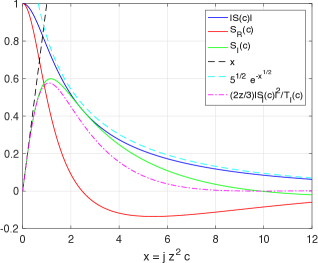
Figure 1: Plot of $|S(c)|$, $S_{R}(c)$, $S_{I}(c)$, and related bounds for $c=-jx/z^{2}$.

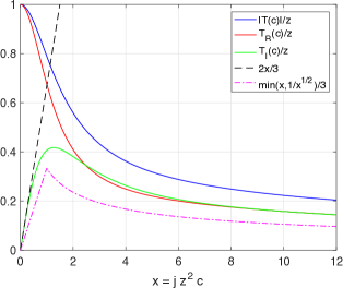
Figure 2: Plot of $|T(c)|/z$, $T_{R}(c)/z$, $T_{I}(c)/z$, and related bounds for $c=-jx/z^{2}$.

III Fiber and OA Noise Models

III-A Nonlinear Schrödinger Equation

Consider the slowly varying component $a(z,T)$ of a single-mode, linearly-polarized, electromagnetic wave $a(z,T)e^{j2\pi f_{0}T}$ along an optical fiber, where $z$ is the position, $T$ is time, and $f_{0}$ is the carrier frequency. The propagation of $a(z,T)$ in the signaling regime of interest is governed by the stochastic NLSE (see [16, Eq. (2.3.27)])

$$\frac{\partial a}{\partial z}+\frac{\alpha}{2}a+\beta_{1}\frac{\partial a}{\partial T}+j\frac{\beta_{2}}{2}\frac{\partial^{2}a}{\partial T^{2}}-j\gamma|a|^{2}a-n=0$$ (30)

where $\alpha$ is the loss coefficient, $\beta_{1}$ is the group velocity, $\beta_{2}$ is the group velocity dispersion parameter, and $\gamma$ is the Kerr coefficient. All of these parameters are frequency dependent in general, but we neglect this dependence for simplicity. The variables $n(z,T)$ are realizations of noise random variables $N(z,T)$ whose characteristics we discuss below in Sec. III-B.

Remark 3

The wave propagation is sometimes defined using the complex conjugate of $a(z,T)$. For example, this approach is used in [2].

Remark 4

For signals with very large power and bandwidth, one should include more effects such as self-steepening and intra-pulse Raman scattering, see [16, Eq. (2.3.33) and (2.3.39)]. We do not consider these effects here.

The NLSE is usually expressed using the retarded time $t=T-\beta_{1}z$ and the amplified signal $u(z,t)=e^{\alpha z/2}a(z,t)$. Inserting these modifications into (30), we have the simplified equation

$$\frac{\partial u}{\partial z}=-j\frac{\beta_{2}}{2}\frac{\partial^{2}u}{\partial t^{2}}+j\gamma|u|^{2}u\,e^{-\alpha z}+n\,e^{\alpha z/2}$$ (31)

where we abuse notation and write $n(z,t)$ for $n(z,t+\beta_{1}z)$. A commonly studied version of (31) has $\alpha=0$ so that

$$\frac{\partial u}{\partial z}=-j\frac{\beta_{2}}{2}\frac{\partial^{2}u}{\partial t^{2}}+j\gamma|u|^{2}u+n.$$ (32)

The model (32) has many interesting features. For example, if $\beta_{2}<0$ and there is no noise, i.e., $n(t)=0$ for all $t$, then the fiber supports bright solitons, see  [16, Ch. 5]. However, the general model seems to have no closed-form solution and, to gain insight, one often studies channels without nonlinearity ($\gamma=0)$ or without dispersion ($\beta_{2}=0$) or without noise.

III-B OA Noise Model

The signal $n(z,\cdot)$ in (30)-(32) represents OA noise. Two common choices for OA are erbium-doped fiber amplifiers (EDFAs) at specified positions along the fiber and distributed Raman amplification [1, Sec. IX.B]. We consider Raman amplification, and we observe that the noise statistics are rather complex, see Appendix IX. We consider two noise models; the first model is described in this section and is used in Sec. III-C below. The second model is developed in Sec. III-D and is used in the remaining sections to analyze spectral broadening.

The usual approach is to model the OA noise $n(z,\cdot)$ as a bandlimited Gaussian process with the same bandwidth $B$ as the OA bandwidth. The noise is assumed independent across positions $z$ so that we have the spatiotemporal autocorrelation function

$${\rm E}\left[{N(z,t)N(z^{\prime},t^{\prime})^{*}}\right]=K\,\delta(z-z^{\prime})\,{\rm sinc}(B(t-t^{\prime}))$$ (33)

where $K=N_{A}B$ is the noise power distance density (PDD) in W/m, and where $N_{A}$ is the OA noise power spectral-distance density (PSDD) in W/Hz/m.

More precisely, the accumulated noise at time $t$ is modeled as a spatial Wiener process $\sqrt{K}\,W(\cdot,t)$ with $W(z,t)=(W_{R}(z,t)+jW_{I}(z,t))/\sqrt{2}$ where $W_{R}(\cdot,t)$ and $W_{I}(\cdot,t)$ are independent standard real Wiener processes. A useful model is that $W(\cdot,t)$ is the limit for large $\ell$ of the processes

$$W_{\ell}(z,t)=\sum_{i=1}^{\lfloor\ell z\rfloor}\frac{1}{\sqrt{\ell}}N_{i}(t)$$ (34)

where the time processes in the sequence $\{N_{i}(\cdot)\}_{i=1}^{\infty}$ are independent and identically distributed (i.i.d.), complex, circularly-symmetric, bandlimited, Gaussian random processes with mean 0 and autocorrelation function

$${\rm E}\left[{N_{i}(t)N_{i}(t^{\prime})^{*}}\right]={\rm sinc}(B(t-t^{\prime})).$$ (35)

Thus, $W_{\ell}(z,t)$ and $W_{\ell}(z,t^{\prime})$ are correlated in general, and from (34)-(35) we have the correlation coefficient

$$\rho_{\ell}(z,t,t^{\prime}) =\frac{{\rm E}\left[{W_{\ell}(z,t)W_{\ell}(z,t^{\prime})^{*}}\right]}{\sqrt{{\rm E}\left[{|W_{\ell}(z,t)|^{2}}\right]{\rm E}\left[{|W_{\ell}(z,t^{\prime})|^{2}}\right]}}$$

$$={\rm sinc}(B(t-t^{\prime})).$$ (36)

Observe that (36) is independent of $\ell$, $z$, and the absolute time $t$, so we use the notation $\rho(t-t^{\prime})$ instead of $\rho_{\ell}(z,t,t^{\prime})$.

III-C Lossless and Linear Fiber Model

Consider (32) but with $\gamma=0$. Taking Fourier transforms, the propagation equation is

$$\frac{\partial\tilde{u}}{\partial z}=j\frac{\beta_{2}}{2}(2\pi f)^{2}\tilde{u}+\tilde{n}$$ (37)

where $\tilde{u}(z,\cdot)$ and $\tilde{n}(z,\cdot)$ are the respective Fourier transforms of $u(z,\cdot)$ and $n(z,\cdot)$. The solution of (37) is

$$\tilde{u}(z,f)=\tilde{u}(0,f)\,e^{j\frac{\beta_{2}}{2}(2\pi f)^{2}z}+\sqrt{K}\tilde{w}(z,f)$$ (38)

where $\tilde{w}(z,\cdot)$ is the Fourier transform of $w(z,\cdot)$. Using the noise model described in Sec. III-B, the process $\tilde{w}(\cdot,f)$ is a realization of a spatial Wiener process if $|f|<B/2$, and is zero otherwise.The channel filter is therefore an all-pass filter with phase shifts proportional to $f^{2}$; the frequency-dependence of the phase is called chromatic dispersion. Furthermore, the channel is noise-free outside the band $|f|<B/2$. This property is problematic when considering information theoretic limits of communication, see Sec. IV-A below.

III-D Lossless and Dispersion-Free Fiber Models

Consider (32) but without dispersion. We have

$$\frac{\partial u}{\partial z}=j\gamma|u|^{2}u+n.$$ (39)

The formal solution of (39) is (see [2, eq. (11)])

$$u =\left[u_{0}+\sqrt{K}\,\hat{w}\right]\exp\left[j\gamma\int_{0}^{z}\left|u(z^{\prime},t)\right|^{2}dz^{\prime}\right]$$ (40)

where the accumulated noise is

$$\hat{w}(z,t)=\int_{0}^{z}n(z^{\prime},t)\exp\left[-j\gamma\int_{0}^{z^{\prime}}\left|u(z^{\prime\prime},t)\right|^{2}dz^{\prime\prime}\right]dz^{\prime}.$$ (41)

Suppose that $n(z,t)$ is Gaussian with uniform phase and is spatially white, as described in Sec. III-B. This means that $\hat{w}(\cdot,t)$ is a realization of a spatial Wiener process that is independent of $u_{0}(t)$, see [2, eq. (13)]. One may thus write the sampled output (40) explicitly as

$$u(z,t) =\left[u_{0}(t)+\sqrt{K}\,w(z,t)\right]$$

$$\quad\exp\left[j\gamma\int_{0}^{z}\left|u_{0}(t)+\sqrt{K}w(z^{\prime},t)\right|^{2}dz^{\prime}\right]$$ (42)

where $w(\cdot,t)$ is a spatial Wiener noise process.

However, the autocorrelation $A_{z}(t,t^{\prime})$ involves the statistics of two samples $u(z,t)$ and $u(z,t^{\prime})$, and the processes $\hat{w}(\cdot,t)$ and $\hat{w}(\cdot,t^{\prime})$ that define these respective samples might not be jointly Wiener. The reason is that the exponential in (41) decorrelates the noise, i.e., the temporal noise process $\hat{w}(z,\cdot)$ also experiences spectral broadening. As an additional complication, the noise model of Sec. III-B may not be accurate for Raman scattering because the coupling of the pump and propagating signals also decorrelates the noise. We address Raman scattering in Appendix IX.

To circumvent the difficulties, and to permit analysis, we study the model (42) where $w(\cdot,t)$ and $w(\cdot,t^{\prime})$ are jointly Wiener processes for any $t$ and $t^{\prime}$. This model seems reasonable for small $\gamma$, $K$, $z$, and $P$, but accumulated noise with exponential terms such as in (41) deserve more study.

As a final remark, if we expand the quadratic term of the exponential in (42), then we obtain three parts: a self-phase modulation term $|u(0,t)|^{2}$, a signal-noise mixed term $2\sqrt{K}\Re\{u(0,t)w(z^{\prime},t)^{*}\}$, and a noise term $K|w(z^{\prime},t)|^{2}$. If $|u(0,t)|$ is large, then the signal-noise mixed term will cause large and random phase variations that result in uncontrolled spectral broadening. Understanding this effect seems key to understanding the nonlinear Shannon limit of optical fiber, i.e., the limitation of the capacity [1].

IV Receiver Models

This section reviews two classes of receiver models. The first class is the per-sample models studied in [2, 3, 4, 5, 6, 7]. The second class is the filter-and-sample models that are commonly used in information theory [17, Ch. 8.1]. For the latter models, we will study receivers that we consider to be of engineering relevance, namely bandlimited receivers and time-resolution limited receivers, both with thermal noise.

IV-A Per-Sample Model and Unbounded Capacity

The capacity of the channel (38) is well-understood. For example, if the launch signal $\tilde{u}(0,\cdot)$ can have energy outside the noise band, then the capacity is unbounded for any launch power [12, Thm. 5]. The purpose of this section is to show that the nonlinear model (42) can also have unbounded capacity, which suggests that the per-sample model gives limited insight for realistic receivers, see Sec. I-A.

Consider $T\leq 1/B\leq T_{s}$ and the launch signal

$$u(0,t)=x\,g(t-T/2)-2x\,g(t-3T/2)$$ (43)

where $x$ is an information symbol and $g(\cdot)$ is a rectangular pulse of unit norm in the interval $[0,T_{s})$. We claim that, for small $T$, the launch bandwidth is described mainly by $T_{s}$ and not $T$. We have

$$|\tilde{u}(0,f)|=|x|\cdot\left|\tilde{g}(f)\right|\cdot\sqrt{5-4\cos(2\pi fT)}$$ (44)

where $\tilde{g}(\cdot)$ is the Fourier transform of $g(\cdot)$. Choosing small $T$ thus does not increase the launch bandwidth, e.g., if one uses a measure such as the band having 99% of the power.

We now choose $T\ll 1/B$ so that the noise variables at $t=0,\,T,\,2T$ are approximately the same, i.e., we have

$$w(z,0)\approx w(z,T)\approx w(z,2T).$$

We can make the approximations as accurate as desired by choosing sufficiently small $T$. Let $w(z,0)=w_{R}+jw_{I}$ and suppose $x$ is real. We choose a 3-sample receiver that outputs

$$y_{0}=\left|u_{z}(0)\right|^{2}=K\left(w_{R}^{2}+w_{I}^{2}\right)$$ (45)

$$y_{1}=\left|u(z,T)\right|^{2}\approx\left(x/\sqrt{T_{s}}+\sqrt{K}w_{R}\right)^{2}+Kw_{I}^{2}$$ (46)

$$y_{2}=\left|u(z,2T)\right|^{2}\approx\left(-x/\sqrt{T_{s}}+\sqrt{K}w_{R}\right)^{2}+Kw_{I}^{2}$$ (47)

and compute

$$x^{2}\approx T_{s}\left(\frac{y_{1}+y_{2}}{2}-y_{0}\right)$$ (48)

to any desired accuracy by choosing sufficiently small $T$. This means that, for the launch energy $x^{2}(1+4T/T_{s})\approx x^{2}$, we can achieve any rate by choosing sufficiently small $T$. In other words, the capacity is unbounded for any launch power.

Remark 5

The reader might consider this example unsatisfactory because it requires rapid signaling. In fact, the example does not work with sinc pulses, yet it seems artificial to limit attention to such pulses. The main purpose of the example is to show that bandlimited noise has pitfalls when dealing with capacity, and that care is needed in treating bandwidth [18].

Remark 6

The above observations apply also to the full NLSE model of Sec. III-A. For example, at small launch power the channel is basically an AWGN channel with bandlimited noise.

IV-B Filter-and-Sample Model

A natural approach to circumvent the infinite-capacity problem of bandlimited noise is to add AWGN to the nonlinear model (42). In other words, the new model has two noise processes: the bandlimited distributed OA noise and the receiver AWGN. More precisely, consider a receiver that operates on a noisy signal

$$u_{r}(t)=u(z,t)+n_{r}(t)$$ (49)

where $n_{r}(\cdot)$ is the same as in (8).

Now consider the set $L^{2}[0,T]$ of continuous and finite-energy signals in the time interval $[0,T]$. This set has a complete orthonormal basis $\left\{\phi_{m}(\cdot)\right\}_{m=1}^{\infty}$ and one usually has a receiver that puts out a finite number of projection values

$$Y_{m} =\int_{0}^{T}U_{r}(z,t)\phi_{m}(t)^{*}dt$$

$$=Z_{m}+\int_{0}^{T}U(z,t)\phi_{m}(t)^{*}dt$$ (50)

for $m=1,2,\ldots,M$ where

$$Z_{m} =\int_{0}^{T}N_{r}(t)\phi_{m}(t)^{*}dt.$$ (51)

In other words, $Z_{1},Z_{2},\ldots,Z_{M}$ is a string of statistically independent, complex, circularly-symmetric, Gaussian random variables with variance $N_{0}$. The set $\{Y_{m}\}_{m=1}^{M}$ of measurements forms a set of sufficient statistics if every possible signal $u(z,\cdot)$ lies in the subspace spanned by the signals $\left\{\phi_{m}(\cdot)\right\}_{m=1}^{M}$. Otherwise, one must let $M\rightarrow\infty$ in general. We refer to the above model as the filter-and-sample model to distinguish it from the per-sample model.

Remark 7

An alternative to introducing receiver thermal noise is to assume that $u(z,\cdot)$ has spectral components inside the OA bandwidth only. However, this approach prevents considering finite-time pulses such as rectangular pulses. Furthermore, spectral broadening prevents $u(z,\cdot)$, $z>0$, from remaining strictly bandlimited even if $u(0,\cdot)$ is strictly bandlimited.

Remark 8

A second alternative is to study OA with infinite bandwidth but with a finite PDD of $K$ W/m. Another way to think of this is that the noise PSDD is $N_{A}=K/B$ W/Hz/m and one considers the limit of increasing $B$. This is effectively what was done in [2, Sec. IV], and we develop results for this model in Appendix 4. The model is artificial but it has two useful features: the analysis greatly simplifies and the model gives insight into systems where the optical noise process has much larger bandwidth than the signals propagating along the fiber. Related studies on models with white phase noise can be found in [19, 20, 21].

Remark 9

We show in Appendix 3 that the nonlinearity can increase capacity. The idea is to use the nonlinearity to convert amplitude-shift keying (ASK) to orthogonal frequency-shift keying (FSK). We remark that orthogonal FSK achieves capacity for large bandwidth $W$ [13, p. 207] and that capacity grows linearly in launch power for large $W$, see (12).

IV-C Bandlimited Receiver

We will consider two receivers that are related. The first is bandlimited to $W$ Hz, i.e., the receiver collects energy in the frequency band $f\in[-W/2,W/2]$ only. The average receiver power after filtering is (see (15))

$$\bar{P}_{r}(W) =\int_{-W/2}^{W/2}\bar{\mathcal{P}}(f)\,df.$$ (52)

Note that we have not included the noise $N_{r}(\cdot)$ in $\bar{P}_{r}(W)$; this noise will contribute an additional $WN_{0}$ Watts.

For convenience, we define (see (4))

$$\bar{P}_{r}(W,T)=\int_{-W/2}^{W/2}\bar{\mathcal{P}}(f,T)\,df.$$ (53)

To later help us bound $\bar{P}_{r}(W,T)$, we upper bound the PSD of unit height in the frequency interval $[-W/2,W/2]$ by

$$\tilde{b}(f)=\left\{\begin{array}[]{ll}2\left(1-\frac{|f|}{W}\right),&|f|\leq W\\ 0,&\text{else}.\end{array}\right.$$ (56)

The motivation for this step is to ensure that the absolute value of the corresponding time signal

$$b(t)=2W\,{\rm sinc}\left(Wt\right)^{2}$$ (57)

integrates to a finite value for $t\geq 0$, namely the value

$$\int_{0}^{\infty}|b(t)|\,dt=1.$$ (58)

Inserting (56) into (53), we have

$$\bar{P}_{r}(W,T) \leq\int_{-W}^{W}\bar{\mathcal{P}}(f,T)\,\tilde{b}(f)\,df$$

$$=\frac{1}{T}\int_{-T/2}^{T/2}\int_{-T/2}^{T/2}\bar{A}(t,t^{\prime})\,b(t-t^{\prime})\,dt^{\prime}\,dt.$$ (59)

For cyclostationary signals, we obtain

$$\bar{P}_{r}(W)\leq\int_{-\infty}^{\infty}\bar{A}(\tau)\,b(\tau)\,d\tau.$$ (60)

IV-D Time-Resolution Limited Receiver

The second receiver is time-resolution limited to $T_{r}$ seconds where $T_{r}\leq T_{s}$. More precisely, we consider a normalized integrate-and-dump filter over $T_{r}$ seconds. The energy output by the receiver is

$$E_{m}(T_{r}) ={\rm E}\left[\left.\left|\int_{mT_{r}}^{(m+1)T_{r}}\frac{1}{\sqrt{T_{r}}}\,U(t)\,dt\right|^{2}\right|U_{0}(\cdot)=u_{0}(\cdot)\right]$$

$$=\frac{1}{T_{r}}\int_{mT_{r}}^{(m+1)T_{r}}\int_{mT_{r}}^{(m+1)T_{r}}A(t,t^{\prime})\,dt^{\prime}\,dt.$$ (61)

Thus, the average energy is

$$\bar{E}_{m}(T_{r})=\frac{1}{T_{r}}\int_{mT_{r}}^{(m+1)T_{r}}\int_{mT_{r}}^{(m+1)T_{r}}\bar{A}(t,t^{\prime})\,dt^{\prime}\,dt.$$ (62)

The value $\bar{E}_{m}(T_{r})$ is closely related to the right-hand side (RHS) of (59).

Remark 10

One can build a receiver with time-resolution $T_{r}/2$ seconds with two receivers with time resolution $T_{r}$ seconds by offsetting their integration times by $T_{r}/2$ seconds. Thus, it might make more sense to state that our receivers have limited time precision. Similarly, one can build a bandwidth $2W$ receiver with two bandwidth $W$ receivers whose center frequencies are offset by $W$ Hz. Of course, these approaches increase complexity and cost, and in practice one is limited by the available receivers.

V Autocorrelation Function

The following theorem is our main analytic result. Consider

$$c=-j\gamma(K/2)\sqrt{1-\rho^{2}}$$ (63)

so that in Sec. II-E we have $c=-jx/z^{2}$ where

$$x=\gamma(K/2)z^{2}\sqrt{1-\rho^{2}}.$$ (64)

Theorem 1

The conditional autocorrelation function (1) of the signal (42) when $w(\cdot,t)$ and $w(\cdot,t^{\prime})$ are jointly Wiener processes for any $t$ and $t^{\prime}$ is

$$A(t,t^{\prime})=|S(c)|^{2}\Big{[}T_{R}(c)K\rho+$$

$$\qquad\left(S_{R}(c)u_{0}+j\frac{S_{I}(c)}{\sqrt{1-\rho^{2}}}(u_{0}-\rho u_{0}^{\prime})\right)$$

$$\qquad\left.\left(S_{R}(c)u_{0}^{\prime}+j\frac{S_{I}(c)}{\sqrt{1-\rho^{2}}}(u_{0}^{\prime}-\rho u_{0})\right)^{*}\;\right]$$

$$\quad\exp\left(j\gamma\,T_{R}(c)\left[|u_{0}|^{2}-|u_{0}^{\prime}|^{2}\right]\right)$$

$$\quad\exp\left(-\gamma\frac{T_{I}(c)}{\sqrt{1-\rho^{2}}}[|u_{0}|^{2}+|u^{\prime}_{0}|^{2}-2\rho\Re\{u_{0}u_{0}^{\prime*}\}]\right).$$ (65)

Proof:

Expression (65) is derived in Appendix 1 by using the development in [2] that is reviewed in Appendices IX-IX. ∎

Remark 11

The first exponential of (65) describes self-phase modulation (SPM) and the second exponential is due to signal-noise mixing. The argument of the latter exponential is real, non-positive, and decreases with the instantaneous powers $|u_{0}|^{2}$ and $|u_{0}^{\prime}|^{2}$ of the launch signal unless $t=t^{\prime}$.

Example 1

Consider $\gamma=0$ so the channel is linear. We have $c=0$, $S(c)=1$, $T(c)=z$, and therefore

$$A(t,t^{\prime}) =Kz\rho(t-t^{\prime})+u_{0}(t)u_{0}(t^{\prime})^{*}.$$ (66)

Example 2

Consider $t=t^{\prime}$ so that $u_{0}=u_{0}^{\prime}$, $\rho=1$, $c=0$, $S(c)=1$, $T(c)=z$, and therefore

$$A(t,t) ={\rm E}\left[{\left.|U_{z}(t)|^{2}\right|U_{0}(t)=u_{0}(t)}\right]$$

$$=Kz+|u_{0}(t)|^{2}.$$ (67)

The instantaneous power is thus preserved, see (42).

Example 3

Consider $u_{0}(t)=0$ for all $t$. The noise autocorrelation function is

$$A(t,t^{\prime})=|S(c)|^{2}T_{R}(c)K\rho$$ (68)

and for $t\neq t^{\prime}$ the value $|A(t,t^{\prime})|$ first increases but eventually decreases as $z$ grows. This means that the noise PSD eventually broadens with $z$. However, one usually operates in regimes where $|c|$ is small so that $A(t,t^{\prime})\approx K\rho z$.

Example 4

Consider $u_{0}(t)=\sqrt{P}e^{j\phi(t)}$ for all $t$, i.e., the launch signal has constant envelope. We compute

$$A(t,t^{\prime})$$

$$=|S|^{2}\left[T_{R}K\rho+Pe^{j\phi_{\Delta}}\left(S_{R}^{2}+\frac{S_{I}^{2}}{1-\rho^{2}}\left(1-\rho\,e^{-j\phi_{\Delta}}\right)^{2}\right)\right]$$

$$\quad\exp\left(-\gamma\frac{T_{I}}{\sqrt{1-\rho^{2}}}2P\left[1-\rho\cos(\phi_{\Delta})\right]\right)$$ (69)

where $\phi_{\Delta}(t,t^{\prime})=\phi(t)-\phi(t^{\prime})$, and where we have suppressed the dependence on $c$, $t$, and $t^{\prime}$ for notational convenience.

V-A Low Noise-Nonlinearity-Distance Product

A commonly studied regime is where the noise and/or the Kerr coefficient are small with respect to the distance. More precisely, we consider $\sqrt{\gamma Kz^{2}}$ small enough so that

$$S(c)\approx 1-2c(z^{2}/2)=1+j\gamma K\sqrt{1-\rho^{2}}(z^{2}/2)$$ (70)

$$T(c)\approx z-2c(z^{3}/3)=z+j\gamma K\sqrt{1-\rho^{2}}(z^{3}/3)$$ (71)

are accurate approximations for the various constants in (65). The autocorrelation function is thus approximately

$$\mathcal{A}(t,t^{\prime})=\left(K\rho z+u_{0}u_{0}^{\prime*}+j\gamma K\rho\frac{z^{2}}{2}\left[|u_{0}|^{2}-|u_{0}^{\prime}|^{2}\right]\right)$$

$$\quad\quad\exp\left(+j\gamma z\left[|u_{0}|^{2}-|u_{0}^{\prime}|^{2}\right]\right)$$

$$\quad\quad\exp\left(-\frac{\kappa}{2}[|u_{0}|^{2}+|u^{\prime}_{0}|^{2}-2\rho\Re\{u_{0}u_{0}^{\prime*}\}]\right)$$ (72)

where

$$\kappa=2\gamma^{2}Kz^{3}/3$$ (73)

and where we have kept up to second oder terms in $\sqrt{\gamma Kz^{2}}$.

V-B Bounds on the Autocorrelation Amplitude

Consider the argument of the last exponential in (65) for which we have

$$|u_{0}|^{2}+|u^{\prime}_{0}|^{2}-2\rho\Re\{u_{0}u_{0}^{\prime*}\}$$

$$\quad=|u_{0}^{\prime}-\rho u_{0}|^{2}+|u_{0}|^{2}\left(1-\rho^{2}\right).$$ (74)

Now suppose that $|u_{0}|\geq|u_{0}^{\prime}|$ so that

$$\begin{array}[]{l}|u_{0}-\rho u_{0}^{\prime}|\leq 2|u_{0}|\\ |u_{0}^{\prime}-\rho u_{0}|\leq 2|u_{0}|.\end{array}$$ (77)

We may use (74) and (77) with (22) to bound

$$|A(t,t^{\prime})| \leq\left[Kz+|u_{0}|^{2}\left(1+2\frac{|S_{I}(c)|}{\sqrt{1-\rho^{2}}}\right)^{2}\right]$$

$$\quad\exp\left(-\gamma\,T_{I}(c)\,|u_{0}|^{2}\sqrt{1-\rho^{2}}\right)$$

$$\leq\left[Kz+|u_{0}|^{2}\left(1+\gamma Kz^{2}\right)^{2}\right]$$

$$\quad\exp\left(-\gamma\,T_{I}(c)\,|u_{0}|^{2}\sqrt{1-\rho^{2}}\right).$$ (78)

We further have $\gamma Kz^{2}\approx 0.017$ for certain parameter ranges that we are interested in, see Table I.

Remark 12

The amplitude $|A(t,t^{\prime})|$ captures the influence of signal-noise mixing, but it removes the SPM exponential in (65). The reason for focussing on signal-noise mixing is because this effect cannot be controlled, other than by reducing power, as opposed to the deterministic effects of SPM and cross-phase modulation (XPM). However, in a network environment, the XPM cannot necessarily be controlled either, and interference can be the main limitation on capacity [1].

The bound (78) is useful when $B$ and $K=BN_{A}$ are fixed. However, we will also be interested in scaling $B$ with the launch power. To treat such cases, we keep the $|S(c)|^{2}$ term from (65). We further use (74) and its symmetric counterpart to write

$$|u_{0}|^{2}+|u^{\prime}_{0}|^{2}-2\rho\Re\{u_{0}u_{0}^{\prime*}\}$$

$$=\frac{|u_{0}^{\prime}-\rho u_{0}|^{2}+|u_{0}-\rho u_{0}^{\prime}|^{2}}{2}+\frac{|u_{0}|^{2}+|u_{0}^{\prime}|^{2}}{2}\left(1-\rho^{2}\right).$$ (79)

We now use (22) to bound

$$|A(t,t^{\prime})|\leq|S(c)|^{2}\Big{[}Kz+$$

$$\quad\left(|u_{0}|+\frac{|S_{I}(c)|}{\sqrt{1-\rho^{2}}}\left|u_{0}-\rho u_{0}^{\prime}\right|e^{-\gamma\frac{T_{I}(c)}{\sqrt{1-\rho^{2}}}\frac{|u_{0}-\rho u_{0}^{\prime}|^{2}}{2}}\right)$$

$$\quad\left.\left(|u_{0}^{\prime}|+\frac{|S_{I}(c)|}{\sqrt{1-\rho^{2}}}\left|u_{0}^{\prime}-\rho u_{0}\right|e^{-\gamma\frac{T_{I}(c)}{\sqrt{1-\rho^{2}}}\frac{|u_{0}^{\prime}-\rho u_{0}|^{2}}{2}}\right)\;\right]$$

$$\quad\exp\left(-\gamma\,T_{I}(c)\frac{|u_{0}|^{2}+|u^{\prime}_{0}|^{2}}{2}\sqrt{1-\rho^{2}}\right).$$ (80)

Applying (294) in Appendix IX, we have

$$|A(t,t^{\prime})| \leq|S(c)|^{2}\left[Kz+\left(|u_{0}|+\delta\right)\left(|u_{0}^{\prime}|+\delta\right)\,\right]$$

$$\quad\exp\left(-\gamma\,T_{I}(c)\frac{|u_{0}|^{2}+|u^{\prime}_{0}|^{2}}{2}\sqrt{1-\rho^{2}}\right)$$ (81)

where

$$\delta=\sqrt{\frac{S_{I}(c)^{2}}{e\,\gamma\,T_{I}(c)\sqrt{1-\rho^{2}}}}.$$ (82)

Using (29) with (64), we have

$$\delta \leq\sqrt{\frac{3Kz}{4e}}\approx 1.4\times 10^{-3}$$ (83)

where the approximation is for the parameters of Table I. We here have $|u_{0}|+\delta\approx|u_{0}|$ for “large” signal powers such as $|u_{0}|^{2}\geq 1\times 10^{-3}$ Watts (or 0 dBm).

VI Rectangular Pulses

Consider rectangular pulses, for which the SPM term

$$\exp\left(j\gamma\,T_{R}(c)\left[|u_{0}|^{2}-|u_{0}^{\prime}|^{2}\right]\right)$$

in (65) is unity. Rectangular pulses are thus convenient for studying the spectral broadening characterized by the signal-noise mixing exponential in (65).

Consider the fiber parameters shown in Table I (see [1, Tables I-III]). We have $\sqrt{\gamma Kz^{2}}\approx 0.130$ so that the approximations (70)-(72) are accurate. We further have $\kappa\approx 28.6$ so that the second exponential of (72) is small (less than $1/e$) for power levels beyond $|u_{0}|^{2}=|u_{0}^{\prime}|^{2}=1/\kappa\approx 0.035$ Watts (or 15.4 dBm) if $\rho=0$.

TABLE I: Fiber Parameters

Nonlinear coefficient $\gamma$	1.27 (W-km)-1
Fiber length	2000 km
Temperature $T_{e}$	300 Kelvin
Receiver noise PSD $N_{0}$	$4.142\times 10^{-21}$ W/Hz
OA noise PSDD $N_{A}$	$6.674\times 10^{-24}$ W/Hz/m
OA bandwidth $B$	500 GHz

VI-A Isolated Rectangular Pulse

Consider an isolated rectangular pulse

$$u_{0}(t) =\left\{\begin{array}[]{ll}\sqrt{P},&|t|\leq T_{s}/2\\ 0,&\text{else}\end{array}\right.$$ (86)

that has energy $PT_{s}$ Joules. The approximation (72) is

$$\mathcal{A}(t,t^{\prime})=$$

$$\left\{\begin{array}[]{ll}\left(K\rho z+P\right)e^{-\kappa P(1-\rho)},&|t|\leq\frac{T_{s}}{2},\;|t^{\prime}|\leq\frac{T_{s}}{2}\\ \left(K\rho z+j\gamma K\rho\frac{z^{2}}{2}P\right)e^{j\gamma zP}e^{-\frac{\kappa}{2}P},&|t|\leq\frac{T_{s}}{2},\;|t^{\prime}|>\frac{T_{s}}{2}\\ \left(K\rho z-j\gamma K\rho\frac{z^{2}}{2}P\right)e^{-j\gamma zP}e^{-\frac{\kappa}{2}P},&|t|>\frac{T_{s}}{2},\;|t^{\prime}|\leq\frac{T_{s}}{2}\\ K\rho z,&|t|>\frac{T_{s}}{2},\;|t^{\prime}|>\frac{T_{s}}{2}.\end{array}\right.$$ (91)

For example, for a linear channel we have $\gamma=0$ and

$$\mathcal{A}(t,t^{\prime})=\left\{\begin{array}[]{ll}K\rho z+P,&|t|\leq\frac{T_{s}}{2},\;|t^{\prime}|\leq\frac{T_{s}}{2}\\ K\rho z,&\text{else}.\end{array}\right.$$ (94)

We choose $T_{s}=10$ ps to correspond to the symbol rate of $100$ Gbaud.

Fig. 3 shows $|A(t,t^{\prime})|$ in dB for $t^{\prime}=0$ and $t^{\prime}=5.1$ ps, and for $P=10,100,200,400$ mW. The plot of the amplitude of the approximation (91) is visually indistinguishable from the exact expression (65). At low power, $A(t,0)$ is almost the same as the pulse shape (86) and $A(t,5.1\text{ ps})$ is close to $K\rho z$. However, for $P=10$ mW the function $|A(t,0)|$ already has a small bulge at $t=0$. We have thus entered the nonlinear regime where signal-noise mixing causes spectral broadening. As the power increases further, $10\log_{10}|A(t,0)|$ develops a sinc pulse shape in the range $t=[-5,5]$ ps due to the exponential factor $e^{-\kappa P(1-\rho)}$. The narrow autocorrelation function for $P=400$ mW implies that the spectrum has broadened considerably.

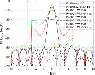
Figure 3: $\left|A(t,t^{\prime})\right|$ in dB for the pulse (86), $t^{\prime}=0$ and $t^{\prime}=5.1$ ps, and $P=10,100,200,400$ mW.

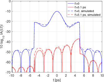
Figure 4: Computed and simulated $\left|A(t,t^{\prime})\right|$ in dB for the pulse (86), $t^{\prime}=0$ and $t^{\prime}=5.1$ ps, and $P=100$ mW.

Fig. 4 shows the exact and simulated autocorrelation functions for $P=100$ mW. The simulated curves are for the averaged $A(t,t^{\prime})$ from $10^{4}$ Monte Carlo simulations of the noise. The curves are in good agreement; note that the y-axis is logarithmic.

VI-B PAM with Rectangular Pulses and Ring Modulation

Consider PAM in (5) with rectangular pulses that are time-limited to $[0,T_{s})$. We study a constant amplitude $\sqrt{P}$, and a phase that is uniformly distributed over $[-\pi,\pi)$, i.e., ring modulation or phase-shift keying (PSK). Using (72) with $u_{0}(t)=\sqrt{P}e^{j\Phi(t)}$ and $u_{0}(t^{\prime})=\sqrt{P}e^{j\Phi(t^{\prime})}$ we have

$$\mathcal{A}(t,t^{\prime}) =\left(K\rho z+Pe^{j\Phi_{\Delta}}\right)e^{-\kappa P\left(1-\rho\cos\Phi_{\Delta}\right)}.$$ (95)

where $\Phi_{\Delta}=\Phi-\Phi^{\prime}$. If $t$ and $t^{\prime}$ are in the same symbol interval, then we have $\Phi_{\Delta}=0$; otherwise $\Phi$ and $\Phi^{\prime}$ are independent and $\Phi_{\Delta}$ is uniform. The average autocorrelation function is therefore

$$\bar{\mathcal{A}}(t,t^{\prime}) =\left\{\begin{array}[]{ll}\left(K\rho z+P\right)e^{-\kappa P\left(1-\rho\right)},&\Phi_{\Delta}=0\\ \left[K\rho z\,I_{0}\left(\kappa P\rho\right)+P\,I_{1}\left(\kappa P\rho\right)\right]e^{-\kappa P},&\text{else}.\end{array}\right.$$ (98)

Note that $\bar{\mathcal{A}}(t,t^{\prime})$ is real-valued. We further compute the time-averaged version of (98) to be (see (6))

$$\bar{\mathcal{A}}(\tau) =\left(1-\frac{|\tau|}{T_{s}}\right)\left(K\rho z+P\right)e^{-\kappa P\left(1-\rho\right)}$$

$$\quad+\frac{|\tau|}{T_{s}}\,\left[K\rho z\,I_{0}\left(\kappa P\rho\right)+P\,I_{1}\left(\kappa P\rho\right)\right]e^{-\kappa P}$$ (99)

for $|\tau|<T_{s}$, and otherwise

$$\bar{\mathcal{A}}(\tau) =\left[K\rho z\,I_{0}\left(\kappa P\rho\right)+P\,I_{1}\left(\kappa P\rho\right)\right]e^{-\kappa P}.$$ (100)

Note that $\bar{\mathcal{A}}(\tau)$ is a real-valued and even function of $\tau$.

A plot of $|\bar{\mathcal{A}}(\tau)|$ is shown in Fig. 5, along with the amplitude of the average autocorrelation function from $10^{4}$ Monte Carlo simulations of the random signals and noise. The simulations were performed using (42) where $w(\cdot,t)$ and $w(\cdot,t^{\prime})$ are jointly Wiener processes for any $t$ and $t^{\prime}$. Observe that $|\bar{\mathcal{A}}(\tau)|$ accurately matches the simulations. The dash-dotted curve is for $\gamma=0$, and it shows that the nonlinearity has caused substantial narrowing of the autocorrelation function, i.e., there is substantial spectral broadening.

This phenomenon is clearly apparent in Fig. 6 that plots the PSDs $\bar{\mathcal{P}}(f)$ for $P=10,50,100,500,1000$ mW, as well as the PSD when $P=10$ mW and $\gamma=0$. Recall that the OA bandwidth is $B=500$ GHz, and observe that $\bar{\mathcal{P}}(f)$ is large well-beyond this frequency already for $P=100$ mW. The model is therefore inaccurate at this launch power since the OA compensates attenuation only for frequencies up to $B$.

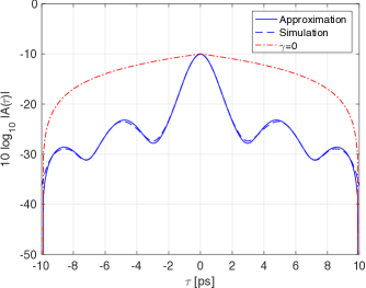
Figure 5: Approximate and simulated $\left|\bar{A}(\tau)\right|$ in dB for PAM with rectangular pulses, ring modulation, and $P=100$ mW. The dash-dotted curve shows $\left|\bar{A}(\tau)\right|$ for the same channel except that $\gamma=0$.

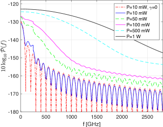
Figure 6: $\bar{\mathcal{P}}(f)$ in dB for PAM with rectangular pulses, ring modulation, and $P=10,50,100,500,1000$ mW. The dash-dotted curve shows $\bar{\mathcal{P}}(f)$ for $P=10$ mW and $\gamma=0$.

Remark 13

The received signal energy is $\bar{A}(0)=\bar{\mathcal{A}}(0)=Kz+P$, and as $\gamma\rightarrow 0$ we have

$$\bar{A}(\tau)\rightarrow\left\{\begin{array}[]{ll}K\rho z+\left(1-\frac{|\tau|}{T_{s}}\right)P,&|\tau|\leq T_{s}\\ K\rho z,&\text{else}.\end{array}\right.$$ (103)

The same limiting expression (103) is valid for $\bar{\mathcal{A}}(\tau)$.

VII Power, Bandwidth, and Energy Bounds

This section studies the power and energy at the output of bandlimited and time-resolution limited receivers. The analysis ultimately lets us bound the propagating signal bandwidth as a function of the launch power. A simple but useful bound for low launch power is

$$\bar{P}_{r}(W,T) \leq\bar{P}_{r}(\infty,T)=Kz+\bar{P}_{T}\leq Kz+P$$ (104)

where the second inequality is from (10).

VII-A Bandlimited Receiver

Consider (59) and split the double integral into three parts: one where $|u_{0}|>|u_{0}^{\prime}|$, one where $|u_{0}|<|u_{0}^{\prime}|$, and one where $|u_{0}|=|u_{0}^{\prime}|$. The first two double integrals are identical due to the symmetry in the arguments of the integrand, i.e., for every pair $(t,t^{\prime})=(t_{1},t_{2})$ where $|u_{0}|>|u_{0}^{\prime}|$ there is a pair $(t,t^{\prime})=(t_{2},t_{1})$ for which $|u_{0}|<|u_{0}^{\prime}|$ and

$$\left|\bar{A}(t_{1},t_{2})\,b(t_{1}-t_{2})\right|=\left|\bar{A}(t_{2},t_{1})\,b(t_{2}-t_{1})\right|.$$

In other words, using (59) we have

$$\bar{P}_{r}(W,T) \leq\frac{1}{T}\int_{-T/2}^{T/2}\int_{-T/2}^{T/2}|\bar{A}(t,t^{\prime})\,b(t-t^{\prime})|\,dt^{\prime}dt$$

$$=\frac{2}{T}\iint_{\mathcal{I}_{1}}|\bar{A}(t,t^{\prime})\,b(t-t^{\prime})|\,dt^{\prime}dt$$

$$\quad+\frac{1}{T}\iint_{\mathcal{I}_{2}}|\bar{A}(t,t^{\prime})\,b(t-t^{\prime})|\,dt^{\prime}dt$$ (105)

where

$${\mathcal{I}}_{1}=\{(t,t^{\prime}):|u_{0}|>|u_{0}^{\prime}|,\,|t|\leq T/2,\,|t^{\prime}|\leq T/2\}$$ (106)

$${\mathcal{I}}_{2}=\{(t,t^{\prime}):|u_{0}|=|u_{0}^{\prime}|,\,|t|\leq T/2,\,|t^{\prime}|\leq T/2\}.$$ (107)

We further have $|\bar{A}(t,t^{\prime})|=|{\rm E}\left[{A(t,t^{\prime})}\right]|\leq{\rm E}\left[{|A(t,t^{\prime})|}\right]$. Thus, using (81) and $|u_{0}|\geq|u_{0}^{\prime}|$ for all $(t,t^{\prime})\in{\mathcal{I}}_{1}\cup{\mathcal{I}}_{2}$, we have

$$\bar{P}_{r}(W,T) \leq\frac{1}{T}\int_{-T/2}^{T/2}{\rm E}\left[{P_{r}(W,T,t)}\right]\,dt$$ (108)

where

$$P_{r}(W,T,t)=2\left[Kz+\left(\sqrt{P_{t}}+\delta\right)^{2}\right]$$

$$\int_{-T/2}^{T/2}|S(c)|^{2}\exp\left(-\gamma\,T_{I}(c)\frac{P_{t}}{2}\sqrt{1-\rho^{2}}\right)\,\left|b(t-t^{\prime})\right|\,dt^{\prime}$$ (109)

and where we have defined $P_{t}=|u_{0}(t)|^{2}$.

VII-B Bounds on the Instantaneous Received Power

Recall that $W$ is the receiver bandwidth and $B$ is the OA bandwidth. In Appendix 3, we prove the following lemmas that bound the instantaneous received power $P_{r}(W,T,t)$. We distinguish cases where $x\geq 1$ cannot or can occur.

• Lemma 2 applies to the usual case with $W\leq B$ and low noise-nonlinearity-distance product, i.e., $\gamma(K/2)z^{2}\leq 1$.

• Lemma 3 is for $W\leq B$ and $\gamma(K/2)z^{2}\geq 1$.

• Lemma 4 is for $W\geq B$ and $\gamma(K/2)z^{2}\leq 1$.

We do not consider the case $W\geq B$ and $\gamma(K/2)z^{2}\geq 1$ because this case is slightly more complicated than the others, and because we are mainly interested in $W\leq B$.

Lemma 2

If $W\leq B$ and $\gamma(K/2)z^{2}\leq 1$, then we have

$$P_{r}(W,T,t)\leq 4\left[Kz+(\sqrt{P_{t}}+\delta)^{2}\right]$$

$$\left[\frac{2\,W/B}{\sqrt{(\kappa/8)P_{t}}}\frac{\sqrt{\pi}}{2}{\rm erf}\left(\sqrt{(\kappa/8)P_{t}}\right)+5e^{-\sqrt{\gamma Kz^{2}}-(\kappa/9)P_{t}}\right].$$ (110)

Lemma 3

If $W\leq B$ and $\gamma(K/2)z^{2}\geq 1$, then we have

$$P_{r}(W,T,t)\leq 4\left[Kz+(\sqrt{P_{t}}+\delta)^{2}\right]$$

$$\quad\left[\frac{2\,W/B}{\sqrt{(\kappa/8)P_{t}}}\frac{\sqrt{\pi}}{2}{\rm erf}\left(\sqrt{\frac{P_{t}}{3Kz}}\right)\right.$$

$$\qquad\left.+\frac{25\,W/B}{\gamma Kz^{2}}e^{-\frac{1}{\sqrt{18}Kz}P_{t}}+5e^{-\sqrt{\gamma Kz^{2}}-\sqrt{\frac{\gamma}{20K}}P_{t}}\right]$$ (111)

Lemma 4

If $W\geq B$ and $\gamma(K/2)z^{2}\leq 1$, then we have

$$P_{r}(W,T,t)\leq 4\left[Kz+(\sqrt{P_{t}}+\delta)^{2}\right]$$

$$\left[\frac{2\,W/B}{\sqrt{(\kappa/8)P_{t}}}\frac{\sqrt{\pi}}{2}{\rm erf}\left(\sqrt{(\kappa/8)P_{t}}\,\frac{B}{W}\right)\right.$$

$$\left.+\frac{1}{4}\left(1-\frac{B}{W}\right)e^{-(\kappa/8)P_{t}(B/W)^{2}}+5e^{-\sqrt{\gamma Kz^{2}}-(\kappa/9)P_{t}}\right].$$ (112)

Remark 14

The above bounds are valid for any launch signal. The bounds may be very loose, e.g., for launch signals with bandwidth larger than $B$.

Remark 15

We have

$$\begin{array}[]{rl}(\sqrt{\pi}/2)\,{\rm erf}(y)\approx y,&\text{small }|y|\\ {\rm erf}(y)\approx 1,&\text{large }y.\end{array}$$ (115)

Thus, for large $P_{t}$, the received power scales at most as $\sqrt{P_{t}}$ for all the regimes considered in Lemmas 2-4. The power loss factor of $1/\sqrt{P_{t}}$ is due to signal-noise mixing, and the square-root character of the power loss is due to the quadratic behavior of $\rho(t-t^{\prime})={\rm sinc}(B(t-t^{\prime}))$ near $t=t^{\prime}$. The shape of the OA noise PSD thus directly affects the power scaling.

Remark 16

For small $P_{t}$ or small $\gamma$, we know that the instantaneous received power $P_{r}(W,T,t)$ can be $Kz+P_{t}$, as we expect for a memoryless, noisy, linear channel. For example, for small $P_{t}$ the RHS of (110) approaches

$$4\left[Kz+\left(\sqrt{P_{t}}+\delta\right)^{2}\right]\left[2\,\frac{W}{B}+5e^{-\sqrt{\gamma Kz^{2}}}\right].$$ (116)

Note that $W/B$ can be small but the term $5e^{-\sqrt{\gamma Kz^{2}}}$ is larger than one if $\gamma(K/2)z^{2}\leq 1$. However, for $\gamma(K/2)z^{2}\geq 1$ and small $P_{t}$, the RHS of (111) approaches

$$4\left[Kz+\left(\sqrt{P_{t}}+\delta\right)^{2}\right]\left[\frac{29}{\gamma Kz^{2}}\,\frac{W}{B}+5e^{-\sqrt{\gamma Kz^{2}}}\right].$$ (117)

Now the receiver may put out less power than $Kz+P_{t}$ due to the large noise-nonlinearity-distance product.

Remark 17

If $B$ is very large, then the $W/B$ terms in (110)-(112) are small. We may thus encounter $P_{r}(W,T,t)$ with an exponential behavior in $P_{t}$, see Remark 8 and Appendix 4.

Remark 18

The case $W>B$ has the receiver measuring signals in bands where there is no attenuation yet the noise is small, as discussed in the introduction and Sec. IV-A. Moreover, for fixed $P_{t}$, fixed $B$, and large $W$ we approach the regime of the per-sample receiver where (112) becomes

$$P_{r}(\infty,T,t)$$

$$\leq\left[Kz+(\sqrt{P_{t}}+\delta)^{2}\right]\left[9+20e^{-\sqrt{\gamma Kz^{2}}-(\kappa/9)P_{t}}\right].$$ (118)

The correct answer on the RHS of (118) is $Kz+P_{t}$; the extra factors are due to loose bounding steps that were designed for large $P_{t}$.

VII-C Bounds on the Average Received Power

We continue to study the case $W\leq B$ as the range of practical and theoretical interest. We would next like to develop a bound on the average received power $\bar{P}_{r}(W,T)$ as a function of the maximum average launch power $P$, see (10). For this purpose, define the function

$$f(s,P)=\left[Kz+(\sqrt{P}+\delta)^{2}\right]\frac{\sqrt{\pi}}{2}\frac{{\rm erf}(\sqrt{sP})}{\sqrt{sP}}$$ (119)

and an offset power $P_{o}=3(Kz+\delta^{2})$. In Appendix 3, we prove the following lemmas.

Lemma 5

If $W\leq B$ and $\gamma(K/2)z^{2}\leq 1$, then we have

$$\bar{P}_{r}(W,T)\leq c_{1}+\frac{8W}{B}f\left(\frac{\kappa}{8},P+P_{o}\right)$$ (120)

where

$$c_{1} =20\left[Kz+\delta^{2}+\sqrt{\frac{18}{\kappa e}}\delta+\frac{9}{\kappa e}\,\right]e^{-\sqrt{\gamma Kz^{2}}}.$$ (121)

Furthermore, the RHS of (120) is non-decreasing and concave in $P$.

Lemma 6

If $W\leq B$ and $\gamma(K/2)z^{2}\geq 1$, then we have

$$\bar{P}_{r}(W,T)\leq\frac{W}{B}c_{2}+c_{3}+\frac{16(W/B)}{\gamma Kz^{2}}f\left(\frac{1}{3Kz},P+P_{o}\right)$$ (122)

where

$$c_{2} =\frac{100}{\gamma Kz^{2}}\left[Kz+\delta^{2}+\sqrt{\frac{6Kz}{e}}\delta+\frac{\sqrt{18}Kz}{e}\,\right]$$

$$c_{3} =20\left[Kz+\delta^{2}+\left(\frac{80K}{\gamma e^{2}}\right)^{1/4}\delta+\sqrt{\frac{20K}{\gamma e^{2}}}\,\right]e^{-\sqrt{\gamma Kz^{2}}}.$$ (123)

Furthermore, the RHS of (122) is non-decreasing and concave in $P$.

Remark 19

The values $c_{1}$, $c_{2}$, and $c_{3}$ are independent of $P$ and $W$, but they depend on $B$, $\gamma$, and $z$.

Remark 20

The RHSs of (120) and (122) scale as $\sqrt{P}$ for large $P$.

VII-D Propagating Signal Bandwidth

We proceed to develop a bound on the propagating signal bandwidth, which we also write as $W$ (in the previous sections, the parameter $W$ represented the receiver filter bandwidth). We are particularly interested in large $P$ where spectral broadening occurs. We interpret the regime $W\leq B$ as being “practically relevant” and $W>B$ as being “impractical”.

The average total received power for a linear channel is $Kz+P$. Suppose we require that 99% of this power is inside the band $f\in[-W/2,W/2]$, i.e., we require

$$\bar{P}_{r}(W,T)\geq 0.99(Kz+P).$$ (124)

We remark that the value 99% is not crucial; the results below remain valid for any other choice near 100%.

Consider first $W\leq B$ and $\gamma(K/2)z^{2}\leq 1$. Combining (120) and (124), and using ${\rm erf}(y)\leq 1$, we have (see (276))

$$\frac{W}{B} \geq\frac{0.99(Kz+P)-c_{1}}{8f\left(\kappa/8,P+P_{o}\right)}$$ (125)

$$\geq\frac{\left\{0.99(Kz+P)-c_{1}\right\}\sqrt{(\kappa/8)\left(P+P_{o}\right)}}{8\left[Kz+\left(\sqrt{P+P_{o}}+\delta\right)^{2}\right]}.$$ (126)

Thus, for fixed $B$ and large $P$, we find that $W$ scales at least as a constant times $\sqrt{P}$. This means that there is some power threshold for which $W>B$. We conclude that the model loses practical relevance beyond some launch power threshold.

An upper bound on the threshold follows by computing the $P$ for which the RHS of (125) is one. For example, for the parameters in Table I, we compute $P\leq 18.6$ Watts. However, the power 18.6 Watts seems unrealistically large, which suggests that our bounds are very loose. Fig. 6 also suggests that the bound is loose, since there is substantial spectral broadening already at $P=50$ mW. However, recall that the bounds (125)-(126) are valid for any launch signal, and not only PAM with rectangular pulses and ring modulation.

Consider next $W\leq B$ and $\gamma(K/2)z^{2}\geq 1$. Combining (122) and (124), and using ${\rm erf}(y)\leq 1$, we have

$$\frac{W}{B}\geq\frac{0.99(Kz+P)-c_{3}}{c_{2}+\frac{16}{\gamma Kz^{2}}f\left(\frac{1}{3Kz},P+P_{o}\right)}$$ (127)

$$\geq\frac{\left\{0.99(Kz+P)-c_{3}\right\}\sqrt{P+P_{o}}}{c_{2}\sqrt{P+P_{o}}+\sqrt{\frac{512}{\kappa}}\left[Kz+\left(\sqrt{P+P_{o}}+\delta\right)^{2}\right]}.$$ (128)

Thus, for fixed $B$ and large $P$, we again find that $W$ scales at least as a constant times $\sqrt{P}$. We again conclude that the model loses practical relevance beyond some launch power threshold.

VII-E Distributed Amplification Bandwidth

The bounds (125)-(128) let us study whether we can increase the range of practically relevant $P$ by increasing $B$. We show that this is not possible in general. In fact, as $B$ increases we must limit ourselves to progressively smaller $P$, while at the same time dealing with more noise power $Kz=N_{A}Bz$.

We study the following problem. Suppose the OA bandwidth scales as $B=P^{\beta}$ for some non-negative constant $\beta$. For large $P$, we thus study the case $\gamma(K/2)z^{2}\geq 1$ where the relevant bounds are (122) and (127)-(128). Note that $K$, $\kappa$, and $P_{o}$ are proportional to $B$, while $\delta$ is proportional to $\sqrt{B}$. Thus, $c_{2}$ remains a constant and $c_{3}$ vanishes for large $B$. Inserting $B=P^{\beta}$ into (122), the scaling behavior of $\bar{P}_{r}(W,T)$ for large $P$ is bounded as

$$\bar{P}_{r}(W,T)\lesssim\left\{\begin{array}[]{ll}P^{(1-3\beta)/2},&0\leq\beta\leq 1\\ P^{-\beta},&\beta\geq 1.\end{array}\right.$$ (131)

The average receiver power thus decreases with the average launch power if $\beta>1/3$ and $P$ is sufficiently large.

Next, inserting $B=P^{\beta}$ into (127), the scaling behavior of $W$ is bounded as

$$W\gtrsim\left\{\begin{array}[]{ll}P^{(1+3\beta)/2},&0\leq\beta\leq 1\\ P^{2\beta},&\beta\geq 1.\end{array}\right.$$ (134)

The condition $W\leq B$ for large $P$ requires $P^{(1+3\beta)/2}\lesssim P^{\beta}$ for $0\leq\beta\leq 1$, or $P^{2\beta}\lesssim P^{\beta}$ for $\beta\geq 1$, neither of which is possible. We conclude that there is no scaling of $B$ through which we can make the model practically relevant for large launch power.

VII-F Time-Resolution Limited Receiver

Bounds for the time-resolution limited receiver can be developed using the same steps as those for the bandlimited receiver. For instance, using the same steps as in (105) but with (62) rather than (59), we have the analog of (108)-(109), namely

$$\bar{E}_{m}(T_{r}) \leq\frac{1}{T_{r}}\int_{mT_{r}}^{(m+1)T_{r}}{\rm E}\left[{E_{m}(T_{r},t)}\right]\,dt$$ (135)

where

$$E_{m}(T_{r},t)=2\left[Kz+\left(\sqrt{P_{t}}+\delta\right)^{2}\right]$$

$$\quad\int_{mT_{r}}^{(m+1)T_{r}}|S(c)|^{2}\exp\left(-\gamma\,T_{I}(c)\frac{P_{t}}{2}\sqrt{1-\rho^{2}}\right)\,dt^{\prime}.$$ (136)

Next, by following similar steps as (242)-(249) that were used to derive (110), for $T_{r}\geq 1/B$ we have

$$E_{m}(T_{r},t) \leq 4\left[Kz+(\sqrt{P_{t}}+\delta)^{2}\right]$$

$$\quad\left[\frac{1/B}{\sqrt{(\kappa/8)P_{t}}}\frac{\sqrt{\pi}}{2}{\rm erf}\left(\sqrt{(\kappa/8)P_{t}}\right)\right.$$

$$\qquad\left.+5\left(T_{r}-\frac{1}{B}\right)e^{-\sqrt{\gamma Kz^{2}}-(\kappa/9)P_{t}}\right].$$ (137)

Note that there is no extra factor of two in front of the ${\rm erf}(\cdot)$ term, cf. (110), because we do not need to use the filter (56).

For $T_{r}<1/B$, we have

$$E_{m}(T_{r},t) \leq 4\left[Kz+(\sqrt{P_{t}}+\delta)^{2}\right]$$

$$\quad\frac{1/B}{\sqrt{(\kappa/8)P_{t}}}\frac{\sqrt{\pi}}{2}{\rm erf}\left(\sqrt{(\kappa/8)P_{t}}BT_{r}\right)$$ (138)

which is simpler than (111) because there is only one integration interval, rather than four as in Appendix 3, see (260). As before, for large $P_{t}$ the energy $E_{m}(T_{r},t)$ scales at most as $\sqrt{P_{t}}$. The same claim is valid for the average energy $\bar{E}_{m}(T_{r})$ by using the concavity steps in Appendix 3, see (270)-(274).

Remark 21

The time resolution $T_{r}$ must scale to zero at least as fast as $1/\sqrt{P_{t}}$ to have the RHS of (138) scale as $P_{t}$.

Remark 22

Consider PAM and fixed $P_{t}$. As $T_{r}$ decreases to zero, the RHS of (138) becomes

$$4\left[Kz+(\sqrt{P_{t}}+\delta)^{2}\right]T_{r}$$ (139)

which decreases to zero. However, there are $T_{s}/T_{r}$ samples per transmitted symbol, so the energy collected per symbol is proportional to $T_{s}$.

Remark 23

If $\gamma\rightarrow 0$ then the RHS of (138) becomes $4(Kz+P_{t})T_{r}$. This is loose by a factor of four: a factor of two is from the step corresponding to (105), and another factor of two is from the step corresponding to (249)$(b)$ where the interval ${\mathcal{I}}_{1}$ was enlarged. We show in Appendix IX how to improve these steps to obtain the expected $(Kz+P_{t})T_{r}$ for PAM with rectangular pulses, ring modulation, and $T_{r}=T_{s}=1/B$.

VIII Capacity Upper Bounds

The capacity result (16) implies that

$$C(W)/W\leq\log_{2}\left(1+\frac{\bar{P}_{r}(W)}{WN_{0}}\right)\text{ bits/s/Hz}.$$ (140)

We may thus use (104), (120) and (122) to upper bound $C(W)$.

Consider the fiber parameters in Table I and the receiver bandwidth $W=B=500$ GHz. We study both the normalized capacity (140) and the spectral efficiency

$$\eta=\frac{C(W)}{\max(W,W_{\rm min})}\text{ bits/s/Hz}$$ (141)

where $W_{\rm min}$ is the smallest received signal bandwidth that satisfies (125).

Fig. 7 shows the resulting bounds as the curves labeled “Upper bound” and “$\eta$ bound”. We also plot a lower bound from [1, Fig. 36, curve (1)]. This bound was computed for 5 WDM signals, each of bandwidth 100 GHz, but with dispersion and optical filtering (OF). The upper and lower bounds are thus not directly comparable at high launch power. However, at low launch power both channels are basically linear and have the same capacity. We remark that we have shifted the lower bound by $10\log_{10}(5)\approx 7$ dB to the right, since the $\rm P_{in}$ in  [1, Fig. 36] is the power per WDM channel.

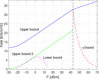
Figure 7: Normalized capacity bounds for dispersion-free fiber with $B=500$ GHz and $W=500$ GHz. The curves “Upper bound” and “$\eta$ bound” are computed with the RHS of (140) and (141), respectively. The curve “Upper bound 2” is computed with the RHS of (143). The lower bound is from [1, Fig. 36, curve (1)].

We comment on the behavior of the curves.

• The upper bound increases with $P$.

• The model is no longer practically relevant according to (125) for $P>18.6$ Watts, or $42.7$ dBm. This bound is shown as the vertical dashed line in Fig. 7. The real threshold for practical relevance is much lower.

• The upper bound has two parts. The part on the left (small to large $P$) up to the vertical dashed line is based on the known bound (104). The part on the right (very large $P$) is new and is based on (120).

• The bound (120) seems useful only when the model is no longer practically relevant. However, this behavior is an artifact of choosing $W=B$; if $W<B$ then (120) can be better than (104) to the left of the power threshold. Furthermore, it is the bound (120) that provides the threshold in the first place.

• The upper bound is far above the lower bound from [1, Fig. 36]. This suggests that the upper bound is very loose.

• The upper bound seems extremely loose for small $P$. To understand why, observe that for small $P$ the RHS of (140) is

  $$\log_{2}\left(1+\frac{Kz}{WN_{0}}\right)\approx 11.7\text{ bits/s/Hz}.$$ (142)

  In fact, we expect that $Kz$ should appear in the denominator of the SNR in (140) and (142), and not in the numerator. This issue is discussed in Sec. VIII-A below.

• Beyond the threshold, $\bar{P}_{r}(W)$ scales as $\sqrt{P}$. The slope of the bound thus changes from approximately 3 dB per bit to 6 dB per bit. However, we expect that the signal phase cannot be used to transmit information at large $P$, cf. [4, Sec. VI.A]. If this is true, then $C(W)/W$ eventually scales at most as $\frac{1}{4}\log P$, and the slope of the upper bound becomes 12 dB per bit.

• The upper bound on (141) decreases rapidly beyond the power threshold because of spectral broadening.

VIII-A Rates with OA Noise

One might expect that a $Kz$ term should appear in the denominator of the SNR in (140). However, we have so far been unable to prove this for the model (42). The difficulty is related to the signal-noise mixing, the bandlimited nature of the OA noise, and to the discussion in Sec. IV-A.

However, suppose the propagating signal remains inside the OA band, as required by the inequality $W\leq B$. Suppose further that the propagating signal is accurately characterized by considering only frequencies within the band $f\in[-W/2,W/2]$ for all $z$. We can then apply the theory in [22, 23] to improve (140) to

$$C(W)/W\leq\log_{2}\left(\frac{\bar{P}_{r}(W)+WN_{0}}{Kz(W/B)+WN_{0}}\right)\text{ bits/s/Hz}.$$ (143)

Consider again the fiber parameters in Table I and $W=B=500$ GHz. Fig. 7 shows the resulting bound on $C(W)/W$ as the curve labeled “Upper bound 2”. We comment on the behavior of the curve.

• The upper bound now seems reasonable for small $P$.

• We do not plot the upper bound or spectral efficiency beyond the power threshold of 42.7 dBm because the signal no longer remains inside the OA band, and hence the theory of [22, 23] does not apply. In fact, substantial spectral broadening occurs at much smaller launch power, so this theory is more limited than suggested by Fig. 7.

VIII-B OA Bandwidth Scales with the Launch Power

Although the models are impractical for large launch power, we can nevertheless follow [3, 4] and study the capacities of the mathematical models for large $P$. For example, suppose $B$ scales as $\sqrt{P}$, which is a lower bound on the spectral broadening scaling, see (134). The motivation for studying this case is to better understand the limitations of spectral broadening. We may use the bounds (120) and (122) to upper bound the receiver power, and we can apply the capacity bounds (140) and (143).

Consider again the fiber parameters in Table I and the receiver bandwidth $W=500$ GHz. However, based on (128) and large $P$, we now scale the OA bandwidth as $B=W\max\left(1,\sqrt{\hat{\kappa}P/512}\right)$ where $\hat{\kappa}=28.6$. Fig. 8 shows the normalized capacity bounds, which are similar to Fig. 7. The main change is that, at high power, both $\bar{P}_{r}(W)$ and $C(W)/W$ scale at most as $P^{-1/4}$, as predicted by (131) with $\beta=1/2$.

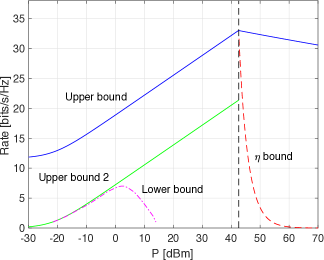
Figure 8: Normalized capacity bounds for dispersion-free fiber with $W=500$ GHz and where $B$ scales as $W\cdot\sqrt{\hat{\kappa}P/512}$ for large $P$. The vertical dashed line is the same one as in Fig. 7.

The reader might expect that the rates in Fig. 8 should not decrease with $P$. However, note that the capacities are normalized, and that the figure is for a system where the OA bandwidth $B$ changes with $P$. In fact, we expect that the real (normalized) capacities at large $P$ will be much smaller than the upper bounds shown in Fig. 7 or Fig. 8.

IX Conclusions

We studied a dispersion-free fiber model with distributed OA where the accumulated spatial noise processes at different time instances are jointly Wiener. Our main result is a closed-form expression for the autocorrelation function of the output signal given the input signal. The expression gives a bound on the output power of bandlimited and time-resolution limited receivers. The theory shows that there is a launch power beyond which the OA bandwidth $B$ can no longer exceed the propagating signal bandwidth $W$, and the model loses practical relevance. The growth of $W$ is due to signal-noise mixing that cannot be controlled by waveform design, other than by reducing power.

The receiver power bounds can be converted to capacity bounds. However, the latter bounds are far above the true capacity, and an interesting problem is to improve them. For example, one can improve the following steps.

• Treat the noise term in (65) separately. An upper bound on the received noise power is $Kz\cdot\min(W/B,1)$.

• Replace (56) with a PSD more like the PSD of unit height in the frequency interval $[-W/2,W/2]$.

• For small $\sqrt{\gamma Kz^{2}}$, replace (28) with a bound similar to $(2/3)xz$.

• For small $\sqrt{\gamma Kz^{2}}$, use (78) rather than (81), since (78) does not have the factor 1/2 inside the exponential. We chose (81) in order to treat large $B$.

• Replace (291) with tighter bounds.

• Use the SPM exponential in (65).

Furthermore, one can improve the bounds for special choices of launch signals, e.g., bandlimited signals or PAM with rectangular pulses, cf. Sec. VI-B and Appendix IX.

Although the bounds are loose, we suspect that they give reasonable guidance on the capacity behavior of NLSE-based fiber models. A challenging open problem is to incorporate the spectral broadening of the noise, see Sec. III-D and Appendix IX. Another challenging problem is to develop autocorrelation functions for NLSE models with noise, nonlinearity, and dispersion. Finally, one may wish to develop autocorrelation functions and capacity bounds for OA based on EDFAs.

Appendix A

Raman Amplification Noise Statistics

We describe a model for Raman amplification based on the coupled NSLEs in [16, p. 305] and [24]. In particular, the paper [24] defines the following signals and constants:

• $u_{p}(z,t)$ and $u_{s}(z,t)$ are the pump and source signals;

• $\gamma_{p}$ and $\gamma_{s}$ are Kerr coefficients at the pump and source frequencies, respectively;

• $\delta_{m}$ is a fraction related to molecular vibrations;

• $g_{p}(t)$ and $g_{s}(t)$ are filters related to the (third-order) nonlinear susceptibility of the fiber medium;

• $h_{p}(t)$ and $h_{s}(t)$ are filters related to the noise force and the response function that converts this force into a spontaneous polarization [24, Sec. II].

The paper derives a set of coupled equations, see [24, Eqs. (12) and (13)]. Setting the dispersion coefficients to zero, we have

$$\frac{\partial u_{p}}{\partial z} =j\gamma_{p}\left(|u_{p}|^{2}+2(1-\delta_{m})|u_{s}|^{2}\right)u_{p}$$

$$\quad+\frac{j}{2}u_{p}u_{s}\,(g_{p}(t)*u_{s}(-t)^{*})+\frac{j}{2}u_{s}\,(h_{p}*n_{w}^{*})$$ (144)

$$\frac{\partial u_{s}}{\partial z} =j\gamma_{s}\left(|u_{s}|^{2}+2(1-\delta_{m})|u_{p}|^{2}\right)u_{s}$$

$$\quad+\frac{j}{2}|u_{p}|^{2}(g_{s}*u_{s})+\frac{j}{2}u_{p}\,(h_{s}*n_{w})$$ (145)

where $n_{w}(z,t)$ is modeled as additive white Gaussian noise.

We simplify (144)-(145) by neglecting $g_{p}(t)*u_{s}(-t)^{*}$, $g_{s}*u_{s}$, and $h_{p}*n_{w}^{*}$; further discussion on modeling can be found in [16, p. 305]. We choose $u_{p}(0,t)=a_{p}$ where $a_{p}$ is a complex constant so that the pump signal is a sinusoid. Solving equations (144)-(145) yields

$$u_{p}(z,t) =a_{p}\exp\left(j\gamma_{p}\left[|a_{p}|^{2}z+2(1-\delta_{m})\phi(z,t)\right]\right)$$ (146)

$$u_{s}(z,t) =\left[u_{s}(0,t)+\hat{w}(z,t)\right]$$

$$\quad\exp\left(j\gamma_{s}\left[\phi(z,t)+2(1-\delta_{m})|a_{p}|^{2}z\right]\right)$$ (147)

where

$$\phi(z,t) =\int_{0}^{z}|u_{s}(z^{\prime},t)|^{2}dz^{\prime}$$ (148)

$$\hat{w}(z,t) =\int_{0}^{z}\frac{j}{2}\,a_{p}\left(h_{s}*n(z^{\prime},t)\right)$$

$$\qquad\exp\left(j|a_{p}|^{2}\left[\gamma_{p}-2(1-\delta_{m})\gamma_{s}\right]z^{\prime}\right)$$

$$\qquad\exp\left(j\phi(z^{\prime},t)\left[-\gamma_{s}+2(1-\delta_{m})\gamma_{p}\right]\right)dz^{\prime}$$ (149)

are the accumulated nonlinear phase and noise.

Note that (41) multiplies $\phi(z^{\prime},t)$ by $-\gamma_{s}$ while (149) multiplies $\phi(z^{\prime},t)$ by $-\gamma_{s}+2(1-\delta_{m})\gamma_{p}$. For example, if $\gamma_{p}=\gamma_{s}$ and $\delta_{m}=1/2$ then the accumulated noise at any two times $t$ and $t^{\prime}$ is jointly Gaussian. However, more realistic numbers are $\gamma_{s}=0.95\gamma_{p}$ and $\delta_{m}=0.2$ (see the text around [24, Eq. (23)]) so that $\phi(z^{\prime},t)$ is multiplied by approximately $0.7\gamma_{s}$.

Appendix B

Cameron-Martin Theory

The purpose of this appendix, as well as Appendices IX and IX is to review relevant results from [25] and [2]. The space $C[0,1]$ is the set of real-valued functions $x(t)$ that are continuous on $t\in[0,1]$ and have $x(0)=0$. Consider the ordered points $t_{1},t_{2},\ldots,t_{n}$ with $0<t_{1}<t_{2}<\ldots<t_{n}\leq 1$ and the values $a_{i}$, $b_{i}$, $i=1,2,\ldots,n$, for which $a_{i}<x(t_{i})<b_{i}$. The Wiener measure is defined as (see [25, p. 73])

$$\frac{1}{\left(\pi^{n}t_{1}(t_{2}-t_{1})\cdots(t_{n}-t_{n-1})\right)^{1/2}}\int_{a_{1}}^{b_{1}}\cdots\int_{a_{n}}^{b_{n}}$$

$$\exp\left(-\frac{s_{1}^{2}}{t_{1}}-\frac{(s_{2}-s_{1})^{2}}{t_{2}-t_{1}}-\cdots-\frac{(s_{n}-s_{n-1})^{2}}{t_{n}-t_{n-1}}\right)ds_{1}\cdots ds_{n}.$$ (150)

The Wiener integral over the space $C[0,1]$ of a functional $F[x]$ is defined using this measure, and the integral is written as

$$\int_{C[0,1]}^{\mathcal{W}}F[x]\,d_{\mathcal{W}}x.$$ (151)

Note that (151) is the same as ${\rm E}\left[{F[X]}\right]$ where $\sqrt{2}\,X(\cdot)$ is a Wiener process on $t\in[0,1]$.

Let $p(t)$ be real-valued, continuous, and positive on $0\leq t\leq 1$ and consider a complex number $\lambda$. Let $\lambda_{0}$ be the least characteristic value of the differential equation

$$f^{\prime\prime}(t)+\lambda\,p(t)f(t)=0$$ (152)

subject to the boundary conditions $f(0)=f^{\prime}(1)=0$. Let $f_{\lambda}(t)$ be any non-trivial solution of (152) satisfying $f_{\lambda}^{\prime}(1)=0$. Let $g(\cdot)$ be a complex-valued and $L^{2}$ function on $0\leq t\leq 1$. We have the following lemma by using Theorem 2 in [25] for real $\lambda$ and real-valued $g(\cdot)$ (see especially (3.2) and (3.3) of [25]). An extension to complex $\lambda$ and $g(\cdot)$ follows by using the same arguments as in [26, pp. 218-219].

Lemma 7 (See [25] and [26])

If $\Re(\lambda)<\lambda_{0}$ then we have

$$\int_{C[0,1]}^{\mathcal{W}}\exp\left(\lambda\int_{0}^{1}\left[p(t)x^{2}(t)+2g(t)x(t)\right]dt\right)d_{\mathcal{W}}x$$

$$=\left(\frac{f_{\lambda}(1)}{f_{\lambda}(0)}\right)^{1/2}\exp\left(\lambda^{2}\beta^{2}\right)$$ (153)

where

$$\beta^{2}=\int_{0}^{1}\left[\frac{1}{f_{\lambda}(t)}\int_{1}^{t}g(s)f_{\lambda}(s)ds\right]^{2}dt.$$ (154)

Example 5 (Example 1 in [25])

If $p(t)=1$ for all $t$, then we have $\lambda_{0}=\pi^{2}/4$. For $\Re(\lambda)<\pi^{2}/4$, we thus have

$$f_{\lambda}(t)=\cos\left(\lambda^{1/2}(t-1)\right).$$ (155)

Appendix C

Mecozzi’s Identity

We prove a (slightly corrected) result from [2, eq. (18)].

Lemma 8 (See [2, eq. (18)])

Consider a standard real Wiener process $W(\cdot)$. For complex numbers $a$ and $b$, and imaginary-valued $c$, we have

$${\rm E}\left[{\exp\left(aW(z)+\int_{0}^{z}bW(z^{\prime})dz^{\prime}-c\int_{0}^{z}W(z^{\prime})^{2}dz^{\prime}\right)}\right]$$

$$=\sqrt{S(c)}\exp\left(\lambda^{2}\beta^{2}\right)$$ (156)

where

$$\lambda^{2}\beta^{2} =\left(\frac{a^{2}}{2}-\frac{b^{2}}{4c}\right)T(c)+\frac{ab}{2c}\left(1-S(c)\right)+\frac{b^{2}}{4c}z.$$ (157)

Proof:

Consider the change of variables $y=z^{\prime}/z$, and write (156) as

$${\rm E}\left[{\exp\left(aW(z)+bz\int_{0}^{1}W(yz)dy-cz\int_{0}^{1}W(yz)^{2}dy\right)}\right]$$

$$={\rm E}\left[\exp\left(a\sqrt{2}z^{1/2}\frac{W(1)}{\sqrt{2}}+b\sqrt{2}z^{3/2}\int_{0}^{1}\frac{W(y)}{\sqrt{2}}dy\right.\right.$$

$$\qquad\qquad\left.\left.-2cz^{2}\int_{0}^{1}\frac{W(y)^{2}}{2}dy\right)\right].$$ (158)

Now consider the function

$$g(s)=\frac{1}{2\lambda}\left(a\sqrt{2}z^{1/2}\frac{1(1-\epsilon\leq s\leq 1)}{\epsilon}+b\sqrt{2}z^{3/2}\right)$$ (159)

where $\epsilon$ is a small positive number. The idea of including the function $1(\cdot)$ is to avoid a Dirac-$\delta$ function, and so that we can write

$$W(1)=\lim_{\epsilon\rightarrow 0}\int_{0}^{1}\frac{1(1-\epsilon\leq s\leq 1)}{\epsilon}\,W(s)\,ds.$$ (160)

We apply (153)-(155) with $\lambda=-2cz^{2}$ and compute

$$\lambda^{2}\beta^{2}=\int_{0}^{1}\left[-\frac{az^{1/2}}{\sqrt{2}}\,\frac{1}{\cos\left(\lambda^{1/2}(t-1)\right)}\,\frac{\sin\left(\lambda^{1/2}\epsilon\right)}{\lambda^{1/2}\epsilon}\right.$$

$$\qquad\qquad\left.+\frac{bz^{3/2}}{\sqrt{2}\lambda^{1/2}}\tan\left(\lambda^{1/2}(t-1)\right)\right]^{2}dt.$$ (161)

For vanishing $\epsilon$, the sine ratio becomes 1, and we have

$$\lambda^{2}\beta^{2} =\frac{a^{2}z}{2\lambda^{1/2}}\tan\left(\lambda^{1/2}\right)-\frac{abz^{2}}{\lambda}\left[1-\frac{1}{\cos\left(\lambda^{1/2}\right)}\right]$$

$$\quad+\frac{b^{2}z^{3}}{2\lambda^{3/2}}\left[\tan\left(\lambda^{1/2}\right)-\lambda^{1/2}\right].$$ (162)

We obtain (156) and (157) by using

$$\tan(jx)=j\tanh(x),\quad\cos(jx)=\cosh(x).$$

∎

Example 6

If $c\rightarrow 0$ then we have

$$\lambda^{2}\beta^{2}\rightarrow\frac{z}{2}\left(a^{2}+ab\,z+\frac{b^{2}}{3}z^{2}\right)$$ (163)

which follows by using the Taylor series expansions

$$\tanh x\approx x-x^{3}/3,\quad\operatorname{sech}x\approx 1-x^{2}/2.$$

Alternatively, one can prove (163) without using (153) by observing that, for $c=0$, the term inside the exponential in (156) is a zero-mean Gaussian random variable.

Appendix D

One-Sample Statistics

We review the sample moments computed in [2, eq. (17)]. As we consider only one time instant $t$, we drop the time variables for convenience of notation.

Recall that $u_{0}=u_{0R}+ju_{0I}$. Consider the conditional moments

$$\mu_{m,n}={\rm E}\left[{\left.U^{m}(U^{*})^{n}\right|U_{0}=u_{0}}\right]$$ (164)

and the moment generating function

$$M_{m,n}(s_{1},s_{2})={\rm E}\left[\exp\left(s_{1}\left[u_{0}+\sqrt{K}W(z)\right]\right.\right.$$

$$\quad+s_{2}\left[u_{0}+\sqrt{K}W(z)\right]^{*}$$

$$\quad\left.\left.+j\gamma(m-n)\int_{0}^{z}|u_{0}+\sqrt{K}W(z^{\prime})|^{2}dz^{\prime}\right)\right]$$ (165)

so that

$$\mu_{m,n}=\left.\frac{\partial^{m+n}}{\partial^{m}s_{1}\,\partial^{n}s_{2}}M_{m,n}(s_{1},s_{2})\right|_{s_{1}=s_{2}=0}.$$ (166)

We compute

$$M_{m,n}(s_{1},s_{2}) =e^{d}\cdot{\rm E}\left[{e^{Z}}\right]$$ (167)

where

$$d=s_{1}u_{0}+s_{2}u_{0}^{*}+j\gamma(m-n)|u_{0}|^{2}z$$ (168)

$$Z=\sqrt{K}\left[s_{1}W(z)+s_{2}W(z)^{*}\right]$$

$$\qquad+j\gamma(m-n)\sqrt{K}\int_{0}^{z}2\,\Re\left\{u_{0}\,W(z^{\prime})^{*}\right\}dz^{\prime}$$

$$\qquad+j\gamma(m-n)K\int_{0}^{z}|W(z^{\prime})|^{2}dz^{\prime}.$$ (169)

Recall that $W(z)=(W_{R}(z)+jW_{I}(z))/\sqrt{2}$, where $W_{R}(\cdot)$ and $W_{I}(\cdot)$ are independent, standard, real, Wiener processes of unit variance. We may thus simplify ${\rm E}\left[{e^{Z}}\right]={\rm E}\left[{e^{A+B}}\right]={\rm E}\left[{e^{A}}\right]{\rm E}\left[{e^{B}}\right]$ where

$$A =\sqrt{\frac{K}{2}}(s_{1}+s_{2})W_{R}(z)$$

$$\qquad+j\gamma(m-n)\sqrt{2K}u_{0R}\int_{0}^{z}W_{R}(z^{\prime})dz^{\prime}$$

$$\qquad+j\gamma(m-n)\frac{K}{2}\int_{0}^{z}W_{R}(z^{\prime})^{2}dz^{\prime}$$ (170)

$$B =j\sqrt{\frac{K}{2}}(s_{1}-s_{2})W_{I}(z)$$

$$\qquad+j\gamma(m-n)\sqrt{2K}u_{0I}\int_{0}^{z}W_{I}(z^{\prime})dz^{\prime}$$

$$\qquad+j\gamma(m-n)\frac{K}{2}\int_{0}^{z}W_{I}(z^{\prime})^{2}dz^{\prime}.$$ (171)

Now define the values

$$\begin{array}[]{ll}a_{1}=\sqrt{K/2}(s_{1}+s_{2}),&a_{2}=j\sqrt{K/2}(s_{1}-s_{2})\\ b_{1}=j\gamma(m-n)\sqrt{2K}u_{0R},&b_{2}=j\gamma(m-n)\sqrt{2K}u_{0I}\\ c_{1}=c_{2}=c=-j\gamma(m-n)K/2&\end{array}$$ (175)

so that

$$\frac{a_{1}^{2}+a_{2}^{2}}{2}=Ks_{1}s_{2},\qquad\frac{b_{1}^{2}+b_{2}^{2}}{4c}=j\gamma(n-m)|u_{0}|^{2}$$

$$\frac{a_{1}b_{1}+a_{2}b_{2}}{2c}=-\left(s_{1}u_{0}+s_{2}u_{0}^{*}\right).$$

We have the following expression using (156):

$${\rm E}\left[{e^{A}}\right]{\rm E}\left[{e^{B}}\right]=S(c)\exp\Big{[}$$

$$\qquad\left(Ks_{1}s_{2}+j\gamma(m-n)|u_{0}|^{2}\right)T(c)$$

$$\qquad\left.-\left(s_{1}u_{0}+s_{2}u_{0}^{*}\right)\left(1-S(c)\right)\right.$$

$$\qquad-j\gamma(m-n)|u_{0}|^{2}z\;\Big{]}.$$ (176)

This gives a result corresponding to [2, eq. (19)]:

$$M_{m,n}(s_{1},s_{2}) =S(c)\exp\Big{[}\left(s_{1}u_{0}+s_{2}u_{0}^{*}\right)S(c)$$

$$\quad+\left(Ks_{1}s_{2}+j\gamma(m-n)|u_{0}|^{2}\right)T(c)\Big{]}$$ (177)

where $c$ is given in (175). For example, for $m=n$ we have $c=0$ from (175), and therefore $S(c)=1$ and $T(c)=z$. If we further have $m=n=1$, then (166) gives

$$\mu_{1,1} =\left.\frac{\partial^{2}}{\partial s_{1}\,\partial s_{2}}M_{1,1}(s_{1},s_{2})\right|_{s_{1}=s_{2}=0}$$

$$=Kz+|u_{0}|^{2}$$ (178)

as expected from (67).

1 First Moment

The $m$th moment is

$${\rm E}\left[{U^{m}}\right]=\mu_{m,0}=u_{0}^{m}\,E_{m}(c)S(c)^{m+1}.$$ (179)

where $c=-j\gamma mK/2$ and

$$E_{m}(c)=\exp\left(j\gamma m|u_{0}|^{2}T(c)\right).$$ (180)

For example, the first moment has $c=-j\gamma K/2$ and

$${\rm E}\left[{U}\right]=u_{0}\,E_{1}(c)S(c)^{2}.$$ (181)

Now consider small $\sqrt{\gamma Kz^{2}}$ for which (see (70)-(71))

$$T(c)\approx z+j\gamma Kz^{3}/3$$ (182)

$$S(c)^{2}\approx 1.$$ (183)

We thus have

$${\rm E}\left[{U}\right] \approx u_{0}\exp\left(|u_{0}|^{2}\left[j\gamma z-\gamma^{2}Kz^{3}/3\right]\right)$$

$$=u_{0}\exp\left(|u_{0}|^{2}\left[j\gamma z-\kappa/2\right]\right)$$ (184)

where we have used $\kappa=2\gamma^{2}Kz^{3}/3$ as in (73). The first moment thus experiences a power reduction of

$$f(z) =\left|E_{1}(c)S(c)^{2}\right|^{2}\approx\exp\left(-\kappa|u_{0}|^{2}\right).$$ (185)

This matches Mecozzi’s equations (29) and (30) from [2].

Remark 24

The value of the first moment may seem curious from the following perspective. The first moment is

$${\rm E}\left[{[u_{0}+\sqrt{K}W(z)]\exp\left(j\gamma\int_{0}^{z}|u_{0}+\sqrt{K}W(z^{\prime})|^{2}dz^{\prime}\right)}\right]$$ (186)

where $n=1$. A casual guess is that (186) should simplify to

$$u_{0}\,M_{1,0}(0,0) =u_{0}\,{\rm E}\left[{\exp\left(j\gamma\int_{0}^{z}|u_{0}+\sqrt{K}W(z^{\prime})|^{2}dz^{\prime}\right)}\right]$$ (187)

since the term with $\sqrt{K}W(z)$ seems to evaluate to zero. However, the first moment would then be

$$u_{0}\,M_{1,0}(0,0)=u_{0}\,E_{1}(c)S(c).$$

Note that the $S(c)$ term is not squared. In fact, we have

$${\rm E}\left[{\sqrt{K}W(z)\,\exp\left(j\gamma\int_{0}^{z}|u_{0}+\sqrt{K}W(z^{\prime})|^{2}dz^{\prime}\right)}\right]$$

$$=u_{0}\left[S(c)-1\right]E_{1}(c)S(c)$$ (188)

which gives the desired result.

Appendix E

Two-Sample Statistics

We write $u_{0}=u_{0}(t)$, $u_{0}^{\prime}=u_{0}(t^{\prime})$, and similarly for $u(t)=u_{z}(t)$. Consider the conditional moments

$$\mu_{mnk\ell}={\rm E}\left[\left.U^{m}(U^{*})^{n}(U^{\prime})^{k}(U^{\prime*})^{\ell}\right|U_{0}(\cdot)=u_{0}(\cdot)\right]$$ (189)

and the moment generating function

$$M_{mnk\ell}({\bf s})={\rm E}\left[\exp\left(\right.\right.$$

$$\quad\;s_{1}[u_{0}+\sqrt{K}W(z,t)]+s_{2}[u_{0}+\sqrt{K}W(z,t)]^{*}$$

$$+s_{3}[u_{0}^{\prime}+\sqrt{K}W(z,t^{\prime})]+s_{4}[u_{0}^{\prime}+\sqrt{K}W(z,t^{\prime})]^{*}$$

$$+j\gamma\int_{0}^{z}(m-n)\;|u_{0}+\sqrt{K}W(z^{\prime},t)|^{2}$$

$$\quad\quad\left.\left.+(k-\ell)\;|u_{0}^{\prime}+\sqrt{K}W(z^{\prime},t^{\prime})|^{2}dz^{\prime}\right)\right]$$ (190)

where ${\bf s}=[s_{1},s_{2},s_{3},s_{4}]$ so that

$$\mu_{mnk\ell}=\left.\frac{\partial^{m+n+k+\ell}}{\partial^{m}s_{1}\,\partial^{n}s_{2}\,\partial^{k}s_{3}\,\partial^{\ell}s_{4}}M_{mnk\ell}({\bf s})\right|_{{\bf s}={\bf 0}}.$$ (191)

1 Autocorrelation Function

For the autocorrelation function, we choose $mnk\ell=1001$. For simplicity of notation, we replace $s_{4}$ with $s_{2}$ and write

$$M_{1001}(s_{1},s_{2})=e^{d}\cdot{\rm E}\left[{e^{Z}}\right]$$ (192)

where

$$d=s_{1}u_{0}+s_{2}u_{0}^{\prime*}+j\gamma z\left[|u_{0}|^{2}-|u_{0}^{\prime}|^{2}\right]$$ (193)

$$Z=\sqrt{K}\left[s_{1}W(z,t)+s_{2}W(z,t^{\prime})^{*}\right]$$

$$\quad+j\gamma\sqrt{K}\int_{0}^{z}2\Re\left\{u_{0}W(z^{\prime},t)^{*}-u_{0}^{\prime}W(z^{\prime},t^{\prime})^{*}\right\}dz^{\prime}$$

$$\quad+j\gamma K\int_{0}^{z}|W(z^{\prime},t)|^{2}-|W(z^{\prime},t^{\prime})|^{2}dz^{\prime}.$$ (194)

2 Noise

Observe that $W(\cdot,t)$ and $W(\cdot,t^{\prime})$ are correlated complex Wiener processes. Since $W(\cdot,t)$ and $W(\cdot,t^{\prime})$ are circularly symmetric, we may write

$$W(z,t^{\prime})=\rho^{*}\,W(z,t)+\sqrt{1-|\rho|^{2}}\,\tilde{W}(z,t^{\prime})$$ (195)

where the correlation coefficient is

$$\rho={\rm E}\left[{W(z,t)W(z,t^{\prime})^{*}}\right]$$ (196)

and $\tilde{W}(z,t^{\prime})=(\tilde{W}_{R}(z,t^{\prime})+j\tilde{W}_{I}(z,t^{\prime}))/\sqrt{2}$ where $\tilde{W}_{R}(\cdot,t^{\prime})$ and $\tilde{W}_{I}(\cdot,t^{\prime})$ are independent, standard, real, Wiener processes that are jointly independent of $W(\cdot,t)$. Using $\rho=\rho_{R}+j\rho_{I}$, we have $W(\cdot,t^{\prime})=(W_{R}(\cdot,t^{\prime})+jW_{I}(\cdot,t^{\prime}))/\sqrt{2}$ where

$$W_{R}(z,t^{\prime})=\rho_{R}\,W_{R}(z,t)+\rho_{I}W_{I}(z,t)+\sqrt{1-|\rho|^{2}}\,\tilde{W}_{R}(z,t^{\prime})$$

$$W_{I}(z,t^{\prime})=\rho_{R}\,W_{I}(z,t)-\rho_{I}W_{R}(z,t)+\sqrt{1-|\rho|^{2}}\,\tilde{W}_{I}(z,t^{\prime}).$$ (197)

We thus have ${\rm E}\left[{W_{R}(z,t^{\prime})W_{I}(z,t^{\prime})}\right]=0$ as required.

We are particularly interested in real $\rho$, see (36). In this case, we have

$$\begin{array}[]{l}W_{R}(z,t^{\prime})=\rho\,W_{R}(z,t)+\sqrt{1-\rho^{2}}\,\tilde{W}_{R}(z,t^{\prime})\\ W_{I}(z,t^{\prime})=\rho\,W_{I}(z,t)+\sqrt{1-\rho^{2}}\,\tilde{W}_{I}(z,t^{\prime}).\end{array}$$ (200)

Thus, the real and imaginary processes are independent, i.e., $W_{R}(z,\cdot)$ is independent of $W_{I}(z,\cdot)$.

3 Analysis of $Z$

Inserting (200) into (194), we have

$$Z=\sqrt{K}\left[s_{1}W(z,t)+s_{2}\rho W(z,t)^{*}+s_{2}\sqrt{1-\rho^{2}}\,\tilde{W}(z,t^{\prime})^{*}\right]$$

$$\quad+j\gamma\sqrt{K}\int_{0}^{z}2\Re\left\{[u_{0}(t)-u_{0}(t^{\prime})\rho]W(z^{\prime},t)^{*}\right.$$

$$\qquad\quad\left.-u_{0}(t^{\prime})\sqrt{1-\rho^{2}}\,\tilde{W}(z^{\prime},t^{\prime})^{*}\right\}dz^{\prime}$$

$$\quad+j\gamma K\int_{0}^{z}(1-\rho^{2})\left(|W(z^{\prime},t)|^{2}-|\tilde{W}(z^{\prime},t^{\prime})|^{2}\right)$$

$$\qquad\quad-2\Re\left\{\rho\sqrt{1-\rho^{2}}W(z^{\prime},t)\tilde{W}(z^{\prime},t^{\prime})^{*}\right\}dz^{\prime}.$$ (201)

The quadratic form in the last integral is ${\bf W}^{\dagger}{\bf Q}{\bf W}$, where

$${\bf W}=\begin{bmatrix}W(z^{\prime},t)&\tilde{W}(z^{\prime},t^{\prime})\end{bmatrix}^{T}$$ (202)

$${\bf Q}=\begin{bmatrix}1-\rho^{2}&-\rho\sqrt{1-\rho^{2}}\\ -\rho\sqrt{1-\rho^{2}}&-(1-\rho^{2})\end{bmatrix}.$$ (203)

The eigenvalue decomposition is $\bf Q={\bf S}{\bf\Lambda}{\bf S}^{T}$, where

$${\bf\Lambda}=\begin{bmatrix}\lambda_{1}&0\\ 0&\lambda_{2}\end{bmatrix}=\begin{bmatrix}\sqrt{1-\rho^{2}}&0\\ 0&-\sqrt{1-\rho^{2}}\end{bmatrix}$$

$${\bf S}=\begin{bmatrix}{\bf e}_{1}&{\bf e}_{2}\end{bmatrix}=\begin{bmatrix}a&b\\ -b&a\end{bmatrix}$$

with

$$a =\frac{1}{\sqrt{2}}\sqrt{1+\sqrt{1-\rho^{2}}}$$ (204)

$$b =\frac{1}{\sqrt{2}}\sqrt{1-\sqrt{1-\rho^{2}}}\cdot{\rm sgn}(\rho).$$ (205)

Note that ${\bf S}^{T}{\bf S}={\bf I}$, $a^{2}+b^{2}=1$, $a^{2}-b^{2}=\sqrt{1-\rho^{2}}$, and $ab=\rho/2$. The quadratic form of interest is ${\bf W}^{\dagger}\left({\bf S}{\bf\Lambda}{\bf S}^{T}\right){\bf W}$. We thus define

$${\bf V}={\bf S}^{T}{\bf W}$$ (206)

where ${\bf V}=[V_{1}(z^{\prime})\>V_{2}(z^{\prime})]^{T}$ with

$$V_{1}(z^{\prime})=(V_{1R}(z^{\prime})+jV_{1I}(z^{\prime}))/\sqrt{2}$$ (207)

$$V_{2}(z^{\prime})=(V_{2R}(z^{\prime})+jV_{2I}(z^{\prime}))/\sqrt{2}.$$ (208)

Since the columns of ${\bf S}$ are orthonormal, the random processes $V_{1R}(\cdot)$, $V_{1I}(\cdot)$, $V_{2R}(\cdot)$, and $V_{2I}(\cdot)$ are jointly independent standard Wiener. We further have

$${\bf W}={\bf S}{\bf V}=\begin{bmatrix}a&b\\ -b&a\end{bmatrix}{\bf V}$$ (209)

$${\bf W}^{\dagger}{\bf Q}{\bf W}={\bf V}^{\dagger}\begin{bmatrix}\lambda_{1}&0\\ 0&\lambda_{2}\end{bmatrix}{\bf V}.$$ (210)

We expand $Z$ as

$$Z=\left(a_{1R}V_{1R}+a_{1I}V_{1I}\right)+\left(a_{2R}V_{2R}+a_{2I}V_{2I}\right)$$

$$+\int_{0}^{z}\left(b_{1R}V_{1R}+b_{1I}V_{1I}\right)+\left(b_{2R}V_{2R}+b_{2I}V_{2I}\right)dz^{\prime}$$

$$-\int_{0}^{z}\left(c_{1R}V_{1R}^{2}+c_{1I}V_{1I}^{2}\right)+\left(c_{2R}V_{2R}^{2}+c_{2I}V_{2I}^{2}\right)dz^{\prime}$$ (211)

where

$$a_{1R}=\sqrt{\frac{K}{2}}\left(a(s_{1}+s_{2}\rho)-bs_{2}\sqrt{1-\rho^{2}}\right)$$

$$a_{1I}=j\sqrt{\frac{K}{2}}\left(a(s_{1}-s_{2}\rho)+bs_{2}\sqrt{1-\rho^{2}}\right)$$

$$a_{2R}=\sqrt{\frac{K}{2}}\left(b(s_{1}+s_{2}\rho)+as_{2}\sqrt{1-\rho^{2}}\right)$$

$$a_{2I}=j\sqrt{\frac{K}{2}}\left(b(s_{1}-s_{2}\rho)-as_{2}\sqrt{1-\rho^{2}}\right)$$

$$b_{1R}=j\gamma\sqrt{2K}\left(a(u_{0R}-\rho u_{0R}^{\prime})+bu_{0R}^{\prime}\sqrt{1-\rho^{2}}\right)$$

$$b_{1I}=j\gamma\sqrt{2K}\left(a(u_{0I}-\rho u_{0I}^{\prime})+bu_{0I}^{\prime}\sqrt{1-\rho^{2}}\right)$$

$$b_{2R}=j\gamma\sqrt{2K}\left(b(u_{0R}-\rho u_{0R}^{\prime})-au_{0R}^{\prime}\sqrt{1-\rho^{2}}\right)$$

$$b_{2I}=j\gamma\sqrt{2K}\left(b(u_{0I}-\rho u_{0I}^{\prime})-au_{0I}^{\prime}\sqrt{1-\rho^{2}}\right)$$

$$c=c_{1R}=c_{1I}=-c_{2R}=-c_{2I}=-j\gamma\frac{K}{2}\sqrt{1-\rho^{2}}$$

and where $u_{0R}=u_{0R}(t)$, $u_{0I}=u_{0I}(t)$, $u_{0R}^{\prime}=u_{0R}(t^{\prime})$, $u_{0I}^{\prime}=u_{0I}(t^{\prime})$.

4 Moment Generating Function

We use (17), (18), the identities

$$\operatorname{sech}\left(\sqrt{-jx}\right)=\operatorname{sech}\left(\sqrt{jx}\right)^{*}$$

$$\tanh\left(\sqrt{-jx}\right)/\sqrt{-jx}=\left(\tanh\left(\sqrt{jx}\right)\big{/}\sqrt{jx}\right)^{*}$$

for real $x$, and Lemma 8 to calculate

$$M_{1001}(s_{1},s_{2})=e^{d}\,|S(c)|^{2}$$

$$\cdot\exp\left[\left(\frac{a_{1R}^{2}+a_{1I}^{2}}{2}-\frac{b_{1R}^{2}+b_{1I}^{2}}{4c}\right)T(c)\right.+$$

$$\quad\left.\frac{a_{1R}b_{1R}+a_{1I}b_{1I}}{2c}\left(1-S(c))\right)+\frac{b_{1R}^{2}+b_{1I}^{2}}{4c}z\right]$$

$$\cdot\exp\left[\left(\frac{a_{2R}^{2}+a_{2I}^{2}}{2}+\frac{b_{2R}^{2}+b_{2I}^{2}}{4c}\right)T(c)^{*}\right.-$$

$$\quad\left.\frac{a_{2R}b_{2R}+a_{2I}b_{2I}}{2c}\left(1-S(c)^{*}\right)-\frac{b_{2R}^{2}+b_{2I}^{2}}{4c}z\right].$$ (212)

We rewrite (212) as

$$M_{1001}(s_{1},s_{2})=e^{d}\,|S(c)|^{2}\exp\Big{[}T_{R}(c)$$

$$\cdot\left(\frac{a_{1R}^{2}+a_{1I}^{2}+a_{2R}^{2}+a_{2I}^{2}}{2}-\frac{b_{1R}^{2}+b_{1I}^{2}-b_{2R}^{2}-b_{2I}^{2}}{4c}\right)$$

$$+jT_{I}(c)$$

$$\cdot\left(\frac{a_{1R}^{2}+a_{1I}^{2}-a_{2R}^{2}-a_{2I}^{2}}{2}-\frac{b_{1R}^{2}+b_{1I}^{2}+b_{2R}^{2}+b_{2I}^{2}}{4c}\right)$$

$$+\left(1-S_{R}(c)\right)\frac{a_{1R}b_{1R}+a_{1I}b_{1I}-a_{2R}b_{2R}-a_{2I}b_{2I}}{2c}$$

$$-jS_{I}(c)\frac{a_{1R}b_{1R}+a_{1I}b_{1I}+a_{2R}b_{2R}+a_{2I}b_{2I}}{2c}$$

$$\left.+\frac{b_{1R}^{2}+b_{1I}^{2}-b_{2R}^{2}-b_{2I}^{2}}{4c}z\right].$$ (213)

The sums in this expression are

$$\frac{a_{1R}^{2}+a_{1I}^{2}+a_{2R}^{2}+a_{2I}^{2}}{2}=Ks_{1}s_{2}\rho$$

$$\frac{a_{1R}^{2}+a_{1I}^{2}-a_{2R}^{2}-a_{2I}^{2}}{2}=0$$

$$\frac{b_{1R}^{2}+b_{1I}^{2}+b_{2R}^{2}+b_{2I}^{2}}{4c}$$

$$\quad=\frac{-j\gamma}{\sqrt{1-\rho^{2}}}[|u_{0}|^{2}+|u^{\prime}_{0}|^{2}-2\rho\Re\{u_{0}u_{0}^{\prime*}\}]$$

$$\frac{b_{1R}^{2}+b_{1I}^{2}-b_{2R}^{2}-b_{2I}^{2}}{4c}=-j\gamma[|u_{0}|^{2}-|u^{\prime}_{0}|^{2}]$$

$$\frac{a_{1R}b_{1R}+a_{1I}b_{1I}+a_{2R}b_{2R}+a_{2I}b_{2I}}{2c}$$

$$\quad=\frac{1}{\sqrt{1-\rho^{2}}}[s_{1}(\rho u_{0}^{\prime}-u_{0})+s_{2}(u_{0}^{\prime}-\rho u_{0})^{*}\big{]}$$

$$\frac{a_{1R}b_{1R}+a_{1I}b_{1I}-a_{2R}b_{2R}-a_{2I}b_{2I}}{2c}$$

$$\quad=-s_{1}u_{0}-s_{2}u_{0}^{\prime*}.$$

We thus have

$$M_{1001}(s_{1},s_{2})=|S(c)|^{2}$$

$$\cdot\exp\Big{[}T_{R}(c)\cdot\left(Ks_{1}s_{2}\rho+j\gamma[|u_{0}|^{2}-|u^{\prime}_{0}|^{2}]\right)$$

$$-\gamma\frac{T_{I}(c)}{\sqrt{1-\rho^{2}}}[|u_{0}|^{2}+|u^{\prime}_{0}|^{2}-2\rho\Re\{u_{0}u_{0}^{\prime*}\}]$$

$$+S_{R}(c)\left[s_{1}u_{0}+s_{2}u_{0}^{\prime*}\right]$$

$$\left.-j\frac{S_{I}(c)}{\sqrt{1-\rho^{2}}}\left[s_{1}(\rho u_{0}^{\prime}-u_{0})+s_{2}(u_{0}^{\prime}-\rho u_{0})^{*}\right]\right].$$ (214)

Taking derivatives and setting $s_{1}=s_{2}=0$ we obtain the autocorrelation function (65).

Appendix F

Infinite Bandwidth and Finite Power Noise

Consider large $B$ but fixed $K$ as in Remark 8, i.e., we have a noise PDD of $K$ W/m that is independent of $B$. Such infinite bandwidth noise is relatively easy to treat because, conditioned on the input, any two samples $U(t)$ and $U(t^{\prime})$ with $t^{\prime}\neq t$ are statistically independent.

1 Autocorrelation and PSD

We have $\rho=1(t=t^{\prime})$ and use (65) to compute

$$A(t,t^{\prime}) =\left\{\begin{array}[]{ll}Kz+|u_{0}(t)|^{2},&t=t^{\prime}\\ v(t)\,v(t^{\prime})^{*},&t\neq t^{\prime}\end{array}\right.$$ (217)

where (cf. (180) and (181))

$$v(t)=u_{0}(t)E_{1}(c,t)S(c)^{2}$$ (218)

$$E_{1}(c,t)=\exp\left(j\gamma|u_{0}(t)|^{2}T(c)\right)$$ (219)

and $c=-j\gamma K/2$. The PSD is therefore

$$\bar{\mathcal{P}}(f,T) ={\rm E}\left[{\left|\int_{-\infty}^{\infty}\frac{1}{\sqrt{T}}V(t)e^{-j2\pi ft}\,dt\right|^{2}}\right]$$ (220)

where $V(\cdot)$ is the random signal with realization $v(\cdot)$, and where the expectation is over the random launch signal $U_{0}(\cdot)$.

2 A Discrete-Time Model

We develop a discrete-time model. Let $\left\{\phi_{m}(\cdot)\right\}_{m=1}^{\infty}$ be a complete orthonormal basis for $L^{2}[0,T]$. Consider the projection output

$$Y_{m}=\int_{0}^{T}U(t)\phi_{m}(t)^{*}dt$$ (221)

and collect these values in the sequence ${\bf Y}=\{Y_{m}\}_{m=1}^{\infty}$ with energy $\|{\bf Y}\|^{2}=\sum_{m=1}^{\infty}|Y_{m}|^{2}$. We can use (179) and the same steps as in [20, 21] (see also [19, Sec. IV.C-D]) to show that if $U_{0}(\cdot)=u_{0}(\cdot)$, then we have

$$Y_{m} \overset{a.s.}{=}\int_{0}^{T}{\rm E}\left[{\left.U(t)\right|U_{0}(\cdot)=u_{0}(\cdot)}\right]\phi_{m}(t)^{*}dt$$

$$=\int_{0}^{T}E_{1}(c,t)S(c)^{2}u_{0}(t)\phi_{m}(t)^{*}dt$$ (222)

where $E_{1}(c,t)$ is given by (219). In other words, the channel effectively modulates $u_{0}(t)$ by the factor $E_{1}(c,t)S(c)^{2}$. This means there is no phase noise since $E_{1}(c,t)$ is a function of $u_{0}(t)$. Instead, the signal loses energy since $|E_{1}(c,t)S(c)^{2}|<1$ if $|u_{0}(t)|>0$, $\gamma>0$, and $K>0$.

The result (222) suggests that we study the complex-alphabet and continuous-time model

$$Y(t)=E_{1}(c,t)S(c)^{2}u_{0}(t)+N_{r}(t)$$ (223)

where $N_{r}(\cdot)$ is an AWGN process with a one-sided PSD of $N_{0}$ W/Hz. The model (223) has several interesting features. First, an optimal receiver may use matched filtering for signals of the form $u_{0}(t)E_{1}(c,t)$. Moreover, suppose $\sqrt{\gamma Kz^{2}}$ is small so that we have (see (219) and (182))

$$E_{1}(c,t)S(c)^{2}\approx\exp\left(\left[j\gamma z-\kappa/2\right]|u_{0}(t)|^{2}\right)$$ (224)

where $\kappa=2\gamma^{2}Kz^{3}/3$ as in (73). We see that the receiver modulates the phase and amplitude of the received signal as a function of $|u_{0}(t)|^{2}$. In particular, if we use PAM with rectangular pulses that are time-limited to $[0,T_{s})$, then the standard matched filter is optimal but the receiver a-posteriori probability calculation should account for the channel’s symbol-dependent attenuation and phase shift.

3 Capacity Bounds

Consider the channel (223) with an amplitude constraint $|u_{0}(t)|\leq A_{\rm max}=\sqrt{PT_{s}}$. For rectangular pulses, we have

$$C=\max_{X:|X|^{2}\leq P}\frac{1}{T_{s}}\left[h(Y)-\log_{2}(\pi eN_{0})\right]$$

$$\leq\frac{1}{T_{s}}\log_{2}\left(1+\frac{\max_{X:|X|^{2}\leq P}{\rm E}\left[{T_{s}|X|^{2}e^{-\kappa|X|^{2}}}\right]}{N_{0}}\right)$$

$$=\left\{\begin{array}[]{ll}\frac{1}{T_{s}}\log_{2}\left(1+\frac{T_{s}Pe^{-\kappa P}}{N_{0}}\right),&\text{if $P<1/\kappa$}\\ \frac{1}{T_{s}}\log_{2}\left(1+\frac{T_{s}}{\kappa eN_{0}}\right),&\text{else}.\end{array}\right.$$ (227)

The smallest $P$ that achieves the maximal upper bound is $P=1/\kappa$. In fact, the bound on the RHS of (227) can be approached if $A_{\rm max}\rightarrow 0$, cf. [27]. Furthermore, for fixed $P$, we can maximize the RHS of (227) over $T_{s}$ to obtain $T_{s}\rightarrow 0$ and therefore

$$\lim_{T_{s}\rightarrow 0}C\leq\frac{1}{\kappa eN_{0}}\log_{2}(e)\quad\text{bits/s}.$$ (228)

The optimal signaling thus uses very fast pulses, and the capacity $C$ decreases inversely proportional to $\gamma^{2}$, $K$, and $z^{3}$.

Appendix G

Nonlinearity Can Increase Capacity

We show that nonlinearity can increase capacity even with receiver noise. In the absence of OA noise, the model (49) with $u(z,t)$ defined by (42) is

$$u_{r}(t)=u_{0}(t)e^{j\gamma|u_{0}(t)|^{2}}+n_{r}(t).$$ (229)

Suppose the transmitter uses PAM with square-root pulses

$$g(t)=\left\{\begin{array}[]{ll}\sqrt{\frac{t-T_{s}+1}{T_{s}(1-T_{s}/2)}},&t\in[0,T_{s})\\ 0&\text{else}\end{array}\right.$$ (232)

where $T_{s}\leq 1$, see (5). For $\gamma=0$ the capacity is

$$C=\frac{1}{T_{s}}\log_{2}\left(1+\frac{PT_{s}}{N_{0}}\right)\text{ bits/s}.$$ (233)

This capacity can be achieved by scaling and shaping quadrature amplitude modulation (QAM) symbols $x_{k}=x_{R,k}+jx_{I,k}$ where the $x_{R,k}$ and $x_{I,k}$ take on values in $\left\{\pm 1,\pm 3,\ldots\right\}$. Note that the capacity scales as $\log_{2}P$ for large $P$.

Suppose now that $\gamma>0$. The main observation is that the nonlinearity in (229) converts the pulse (232) to a tone whose frequency and power is proportional to $|x_{k}|^{2}$. More precisely, the noise-free output signals have the form

$$u(t)=x_{k}\sqrt{\frac{t-T_{s}+1}{T_{s}(1-T_{s}/2)}}\exp\left(j2\pi h\,|x_{k}|^{2}\,(t-T_{s}+1)\right)$$ (234)

for $t\in[kT_{s},(k+1)T_{s})$, where

$$h=\frac{\gamma}{2\pi T_{s}(1-T_{s}/2)}$$

is a modulation index [13, p. 118]. Suppose we use intensity modulation where we choose the $M$ symbols

$$x_{k}\in\{(2i-1)\Delta:\;i=M+1,M+2,\ldots,2M\}$$ (235)

each with probability $1/M$. The average energy is then $E=(28M^{2}-1)\Delta^{2}/3$. We further choose $\gamma$ so that $hT_{s}$ is a positive integer, e.g., $\gamma=2\pi(1-T_{s}/2)$ so that $hT_{s}=1$. The pulses (234) are then mutually orthogonal: for $x_{\ell}\neq x_{m}$ we have

$$\int_{0}^{T_{s}}\frac{t-T_{s}+1}{T_{s}(1-T_{s}/2)}e^{j2\pi h(|x_{\ell}|^{2}-|x_{m}|^{2})(t-T_{s}+1)}\,dt=0.$$ (236)

The channel has thus converted the ASK signals to orthogonal FSK signals for which the frequency grows with the power.

Next, a standard upper bound on the error probability of signal sets is the union bound [13, p. 185]

$$P_{e}\leq(M-1)\,Q\left(\frac{d_{\rm min}}{\sqrt{2N_{0}}}\right)$$ (237)

where $d_{\rm min}$ is the minimum Euclidean distance between different pulses. Since our FSK signals are mutually orthogonal, the minimum distance corresponds to the signals with $i=M+1$ and $i=M+2$, i.e., we have

$$d_{\rm min}=\sqrt{(2M+1)^{2}+(2M+3)^{2}}\cdot\Delta\geq\sqrt{8}\,M\Delta$$

and therefore

$$P_{e}\leq(M-1)\,Q\left(\frac{2\,M\Delta}{\sqrt{N_{0}}}\right).$$ (238)

We use $R=\log_{2}M$ bits/symbol and $Q(x)\leq e^{-x^{2}/2}$ for positive $x$ to write

$$P_{e}<\exp\left(R\ln 2-\frac{6}{28}\frac{E}{N_{0}}\right).$$ (239)

This bound shows that, for any choice of target error probability $\tilde{P}_{e}$, we can choose the rate as

$$\frac{R}{T_{s}}=\frac{6}{28}\frac{P}{N_{0}}\log_{2}e+\frac{1}{T_{s}}\ln\tilde{P}_{e}\quad\text{bits/s}.$$ (240)

The capacity thus scales linearly with $P$ rather than logarithmically as for $\gamma=0$.

Remark 25

The reason for the capacity gain is because the channel has spread the spectrum of the PAM signal. The gain is thus at the expense of using more frequency resources.

Remark 26

The above example shows that intensity modulation can achieve a capacity that grows linearly with $P$ for large $P$. The per-sample rate $\frac{1}{2}\log P$ from [3, 4] thus underestimates capacity even with AWGN at the receiver.

Remark 27

The channel is artificial because we have assumed the channel is lossless without amplification.

Appendix H

Proofs of Lemmas 2-6

We repeat (109) here for convenience:

$$P_{r}(W,T,t)=2\left[Kz+\left(\sqrt{P_{t}}+\delta\right)^{2}\right]$$

$$\int_{-T/2}^{T/2}|S(c)|^{2}\exp\left(-\gamma\,T_{I}(c)\frac{P_{t}}{2}\sqrt{1-\rho^{2}}\right)\,\left|b(t-t^{\prime})\right|\,dt^{\prime}.$$ (241)

Proof of Lemma 2

Consider $W\leq B$ and $\gamma(K/2)z^{2}\leq 1$. We have $x\leq 1$ (see (64)) and the bound (28) gives

$$\gamma\,T_{I}(c)\geq\gamma\,\frac{z\,x}{3}=(\kappa/4)\sqrt{1-\rho^{2}}.$$ (242)

We further use the crude bounds (291) in Appendix IX to upper bound the exponential of (241) as

$$\exp\left(-\gamma\,T_{I}(c)\frac{P_{t}}{2}\sqrt{1-\rho^{2}}\right)$$

$$\leq\left\{\begin{array}[]{ll}\exp\left(-(\kappa/8)P_{t}\,B^{2}(t-t^{\prime})^{2}\right),&B|t-t^{\prime}|\leq 1\\ \exp\left(-(\kappa/9)P_{t}\right),&B|t-t^{\prime}|>1.\end{array}\right.$$ (245)

We now define

$$\sigma=\sqrt{(\kappa/8)P_{t}}\,B,\quad y=\sigma(t-t^{\prime})$$ (246)

and use the time intervals

$${\mathcal{I}}_{1}=\{t^{\prime}:|t-t^{\prime}|\leq 1/B,\,|t^{\prime}|\leq T/2\}$$ (247)

$${\mathcal{I}}_{2}=\{t^{\prime}:|t-t^{\prime}|>1/B,\,|t^{\prime}|\leq T/2\}$$ (248)

to bound (241) as

$$P_{r}(W,T,t)$$

$$\overset{(a)}{\leq}2\left[Kz+(\sqrt{P_{t}}+\delta)^{2}\right]\left[\int_{\mathcal{I}_{1}}2We^{-\sigma^{2}(t-t^{\prime})^{2}}\,dt^{\prime}\right.$$

$$\qquad\left.+\int_{\mathcal{I}_{2}}|S(c)|^{2}e^{-(\kappa/9)P_{t}}\,|b(t-t^{\prime})|\,dt^{\prime}\right]$$

$$\overset{(b)}{\leq}4\left[Kz+(\sqrt{P_{t}}+\delta)^{2}\right]\left[\int_{0}^{\sigma/B}\frac{2W}{\sigma}e^{-y^{2}}\,dy\right.$$

$$\qquad\left.+\int_{1/B}^{\infty}5e^{-\sqrt{\gamma Kz^{2}}}\,e^{-(\kappa/9)P_{t}}\,|b(\tau)|\,d\tau\right].$$ (249)

Step $(a)$ in (249) follows by using (245), $|b(t-t^{\prime})|\leq 2W$, and $|S(c)|^{2}\leq 1$; step $(b)$ follows by using $\tau=t-t^{\prime}$, inserting (27), and applying the second inequality in (291) to bound $x\leq\gamma(K/2)z^{2}(19/20)$. Evaluating the integrals and using (58) gives

$$P_{r}(W,T,t)\leq 4\left[Kz+(\sqrt{P_{t}}+\delta)^{2}\right]$$

$$\left[\frac{2\,W/B}{\sqrt{(\kappa/8)P_{t}}}\frac{\sqrt{\pi}}{2}{\rm erf}\left(\sqrt{(\kappa/8)P_{t}}\right)+5e^{-\sqrt{\gamma Kz^{2}}-(\kappa/9)P_{t}}\right].$$ (250)

Proof of Lemma 3

Consider $W\leq B$ and $\gamma(K/2)z^{2}\geq 1$. We now have the situation that $x\geq 1$ can occur, so that we need both bounds in (28) depending on the value of $\tau=t-t^{\prime}$. We further need both bounds of (291) in Appendix IX, depending on whether $|\tau|$ is smaller or larger than $1/B$. This leads to four integration regions in general, as described below.

We begin with (291)-(292) to write

$$B|\tau|\leq\sqrt{1-{\rm sinc}^{2}(B\tau)}\leq 2B|\tau|$$ (251)

for $0\leq B|\tau|\leq 1$. Using (64), we thus have

$$\gamma(K/2)z^{2}B|\tau|\leq x\leq\gamma Kz^{2}B|\tau|.$$ (252)

Defining

$$\tau^{*}=1/(\gamma Kz^{2}B)$$ (253)

we have $2\tau^{*}\leq 1/B$ by hypothesis, and (252) gives

$$\begin{array}[]{l}|\tau|\leq\tau^{*}\Rightarrow x\leq 1\\ |\tau|\geq 2\tau^{*}\Rightarrow x\geq 1.\end{array}$$ (256)

We proceed to upper bound $P_{r}(W,T,t)$ by splitting the integral (241) into four parts with $|\tau|\leq\tau^{*}$, $\tau^{*}\leq|\tau|\leq 2\tau^{*}$, $2\tau^{*}\leq|\tau|\leq 1/B$, and $|\tau|>1/B$. Using (28) and (291), we bound the exponential of (241) as

$$\exp\left(-\gamma\,T_{I}(c)\frac{P_{t}}{2}\sqrt{1-\rho^{2}}\right)$$

$$\leq\left\{\begin{array}[]{ll}\exp\left(-(\kappa/8)P_{t}\,B^{2}\tau^{2}\right),&|\tau|\leq\tau^{*}\\ \exp\left(-\sqrt{\frac{\gamma B}{18K}}P_{t}\sqrt{\tau}\right),&2\tau^{*}\leq|\tau|\leq 1/B\\ \exp\left(-\sqrt{\frac{\gamma}{20K}}P_{t}\right),&|\tau|>1/B.\end{array}\right.$$ (260)

For the regime $\tau^{*}\leq|\tau|\leq 2\tau^{*}$, we use as upper bound the sum of the first and second terms on the RHS of (260).

Inserting (260) into (241), and following similar steps as in (246)-(249), we have

$$P_{r}(W,T,t)$$

$$\overset{(a)}{\leq}4\left[Kz+(\sqrt{P_{t}}+\delta)^{2}\right]\left[\int_{0}^{2\sigma\tau^{*}}\frac{2W}{\sigma}e^{-y^{2}}\,dy\right.$$

$$\left.+\int_{\tau^{*}}^{1/B}10We^{-a\sqrt{\tau}}\,d\tau+\int_{1/B}^{\infty}5e^{-\sqrt{\gamma Kz^{2}}-\sqrt{\frac{\gamma}{20K}}P_{t}}\,|b(\tau)|\,d\tau\right]$$

$$\overset{(b)}{\leq}4\left[Kz+(\sqrt{P_{t}}+\delta)^{2}\right]$$

$$\left[\frac{2\,W/B}{\sqrt{(\kappa/8)P_{t}}}\frac{\sqrt{\pi}}{2}{\rm erf}\left(\sqrt{(\kappa/8)P_{t}}\,2B\tau^{*}\right)\right.$$

$$\left.+\frac{20W}{a}\left(\sqrt{\tau^{*}}+\frac{1}{a}\right)e^{-a\sqrt{\tau^{*}}}+5e^{-\sqrt{\gamma Kz^{2}}-\sqrt{\frac{\gamma}{20K}}P_{t}}\right]$$ (261)

where for step $(b)$ we have defined

$$a =\sqrt{\frac{\gamma B}{18\,K}}P_{t}+\sqrt{2\gamma Kz^{2}B}.$$ (262)

Step $(a)$ in (261) used the first inequality in (291) to bound $|S(c)|^{2}$ for the second integral. For step $(b)$, we applied

$$\int_{\tau^{*}}^{1/B}e^{-a\sqrt{\tau}}\,d\tau =\int_{\sqrt{\tau^{*}}}^{1/\sqrt{B}}e^{-at}\,2t\,dt$$

$$\leq\frac{2}{a}\left(\sqrt{\tau^{*}}+\frac{1}{a}\right)e^{-a\sqrt{\tau^{*}}}.$$ (263)

Finally, we use

$$a\geq\max\left(\sqrt{\frac{\gamma B}{18\,K}}P_{t},\sqrt{2\gamma Kz^{2}B}\right)$$ (264)

$$\sqrt{(\kappa/8)P_{t}}\,2B\tau^{*}=\sqrt{\frac{P_{t}}{3Kz}}$$ (265)

to simplify (261) and obtain

$$P_{r}(W,T,t)\leq 4\left[Kz+(\sqrt{P_{t}}+\delta)^{2}\right]$$

$$\quad\left[\frac{2\,W/B}{\sqrt{(\kappa/8)P_{t}}}\frac{\sqrt{\pi}}{2}{\rm erf}\left(\sqrt{\frac{P_{t}}{3Kz}}\right)\right.$$

$$\qquad\left.+\frac{25\,W/B}{\gamma Kz^{2}}e^{-\frac{1}{\sqrt{18}Kz}P_{t}}+5e^{-\sqrt{\gamma Kz^{2}}-\sqrt{\frac{\gamma}{20K}}P_{t}}\right].$$ (266)

Proof of Lemma 4

Consider the case $W\geq B$ and $\gamma(K/2)z^{2}\leq 1$. We again use the bound (242) and the parameters (246) to write

$$P_{r}(W,T,t)$$

$$\leq 4\left[Kz+(\sqrt{P_{t}}+\delta)^{2}\right]\left[\int_{0}^{\sigma/W}\frac{2W}{\sigma}e^{-y^{2}}\,dy\right.$$

$$\left.+\int_{1/W}^{1/B}e^{-\sigma^{2}\tau^{2}}\,|b(\tau)|\,d\tau+5e^{-\sqrt{\gamma Kz^{2}}-(\kappa/9)P_{t}}\right].$$ (267)

We now use $|b(t)|\leq 2(W(\pi t)^{2})^{-1}$ to upper bound the second integral in (267) as follows:

$$\int_{1/W}^{1/B}e^{-\sigma^{2}\tau^{2}}\frac{2}{\pi^{2}W\tau^{2}}\,d\tau\leq e^{-(\kappa/8)P_{t}(B/W)^{2}}\frac{W-B}{4W}.$$ (268)

Inserting into (267), we have

$$P_{r}(W,T,t)\leq 4\left[Kz+(\sqrt{P_{t}}+\delta)^{2}\right]$$

$$\left[\frac{2\,W/B}{\sqrt{(\kappa/8)P_{t}}}\frac{\sqrt{\pi}}{2}{\rm erf}\left(\sqrt{(\kappa/8)P_{t}}\,\frac{B}{W}\right)\right.$$

$$\left.+\frac{1}{4}\left(1-\frac{B}{W}\right)e^{-(\kappa/8)P_{t}(B/W)^{2}}+5e^{-\sqrt{\gamma Kz^{2}}-(\kappa/9)P_{t}}\right].$$ (269)

Proof of Lemma 5

Observe that the RHS of (250) includes the form

$$f(P_{t})=(a+b\sqrt{P_{t}}+cP_{t})\frac{\sqrt{\pi}}{2}\frac{{\rm erf}(\sqrt{sP_{t}})}{\sqrt{sP_{t}}}$$ (270)

where $a=Kz+\delta^{2}$, $b=2\delta$, $c=1$, and $s=\kappa/8$. The results (296)-(297) derived in Appendix IX state that (270) is non-decreasing and concave in $P_{t}$ if $P_{t}\geq 3(Kz+\delta^{2})$. Thus, if we replace $P_{t}$ with $P_{t}+P_{o}$, where the offset power is $P_{o}=3(Kz+\delta^{2})$, then (270) is non-decreasing and concave for $P_{t}\geq 0$.

Next, by using (293)-(294) in Appendix IX, we have

$$20\left[Kz+(\sqrt{P_{t}}+\delta)^{2}\right]e^{-\sqrt{\gamma Kz^{2}}-(\kappa/9)P_{t}}\leq c_{1}$$ (271)

where

$$c_{1} =20\left[Kz+\delta^{2}+\sqrt{\frac{18}{\kappa e}}\delta+\frac{9}{\kappa e}\,\right]e^{-\sqrt{\gamma Kz^{2}}}.$$ (272)

Observe that $c_{1}$ is independent of $P_{t}$ and $W$.

We now loosen (250) to

$$P_{r}(W,T,t)\leq c_{1}+8(W/B)f\left(P_{t}+P_{o}\right)$$ (273)

where the RHS is non-decreasing and concave in $P_{t}$. Jensen’s inequality applied to the RHS of (108) thus gives the bound

$$\bar{P}_{r}(W,T)\leq c_{1}+8(W/B)f\left(\bar{P}_{T}+P_{o}\right)$$ (274)

where we have replaced $P_{t}$ with $\bar{P}_{T}$, see (10). Furthermore, we require $\bar{P}_{T}\leq P$, so we have

$$\bar{P}_{r}(W,T)\leq c_{1}+8(W/B)f\left(P+P_{o}\right).$$ (275)

We may simplify the bound further without changing the scaling behavior that we are interested in. We use ${\rm erf}(y)\leq 1$ and loosen (275) to

$$\bar{P}_{r}(W,T)\leq c_{1}+\frac{8W}{B}\frac{Kz+\left(\sqrt{P+P_{o}}+\delta\right)^{2}}{\sqrt{(\kappa/8)\left(P+P_{o}\right)}}.$$ (276)

For example, the RHS of (276) scales as $\sqrt{P}$ for large $P$.

Proof of Lemma 6

We repeat the above steps (270)-(276) for (266). We now have $s=1/(3Kz)$ in (270), and we use (293)-(294) to compute

$$\frac{100}{\gamma Kz^{2}}\left[Kz+(\sqrt{P_{t}}+\delta)^{2}\right]e^{-\frac{1}{\sqrt{18}Kz}P_{t}} \leq c_{2}$$

$$20\left[Kz+(\sqrt{P_{t}}+\delta)^{2}\right]e^{-\sqrt{\gamma Kz^{2}}-\sqrt{\frac{\gamma}{20K}}P_{t}} \leq c_{3}$$ (277)

where

$$c_{2} =\frac{100}{\gamma Kz^{2}}\left[Kz+\delta^{2}+\sqrt{\frac{6Kz}{e}}\delta+\frac{\sqrt{18}Kz}{e}\,\right]$$

$$c_{3} =20\left[Kz+\delta^{2}+\left(\frac{80K}{\gamma e^{2}}\right)^{1/4}\delta+\sqrt{\frac{20K}{\gamma e^{2}}}\,\right]e^{-\sqrt{\gamma Kz^{2}}}.$$ (278)

Observe that $c_{2}$ and $c_{3}$ are independent of $P_{t}$ and $W$. We loosen (266) and use Jensen’s inequality to write

$$\bar{P}_{r}(W,T) \leq\frac{W}{B}c_{2}+c_{3}+\frac{16(W/B)}{\gamma Kz^{2}}f\left(\bar{P}_{T}+P_{o}\right)$$ (279)

which is the analog of (274). The RHS of (279) is increasing in $\bar{P}_{T}$, so we have

$$\bar{P}_{r}(W,T) \leq\frac{W}{B}c_{2}+c_{3}+\frac{16(W/B)}{\gamma Kz^{2}}f\left(P+P_{o}\right).$$ (280)

To study large $P$, we may simplify (280) by again using ${\rm erf}(y)\leq 1$. We arrive at a similar bound as (276), and $\bar{P}_{r}(W,T)$ again scales at most as $\sqrt{P}$ for large $P$.

Appendix I

Energy Bound for PAM with Rectangular Pulses and Ring Modulation

PAM with rectangular pulses and ring modulation has a constant envelope, so we can apply (69). Suppose $T_{r}=T_{s}$, so that for $mT_{r}\leq t,t^{\prime}<(m+1)T_{r}$, we have $\phi_{\Delta}(t,t^{\prime})=0$ and

$$\bar{A}(t,t^{\prime})=A(t,t^{\prime})$$

$$=|S|^{2}\left[T_{R}K\rho+P\left(S_{R}^{2}+\frac{S_{I}^{2}}{1-\rho^{2}}\left(1-\rho\right)^{2}\right)\right]$$

$$\qquad\exp\left(-\gamma\frac{T_{I}}{\sqrt{1-\rho^{2}}}2P(1-\rho)\right).$$ (281)

Note that (281) is real-valued. Using (62) rather than (59), we thus have (cf. (78))

$$\bar{E}_{m}(T_{r})\leq\frac{1}{T_{r}}\left[Kz+P\left(1+\gamma^{2}K^{2}z^{4}\right)\right]$$

$$\quad\int_{0}^{T_{r}}\int_{0}^{T_{r}}\exp\left(-\gamma\frac{T_{I}}{\sqrt{1-\rho^{2}}}2P(1-\rho)\right)\,dt^{\prime}\,dt.$$ (282)

Consider $T_{r}=1/B$ and $\gamma(K/2)z^{2}\leq 1$. We use (242) and (291) to upper bound the exponential of (282) with

$$\exp\left(-(\kappa/2)\,P\,B^{2}(t-t^{\prime})^{2}\right)$$ (283)

for the range of interest with $B|t-t^{\prime}|\leq 1$. We thus have

$$\bar{E}_{m}(T_{r})\leq\frac{1}{T_{r}}\left[Kz+P\left(1+\gamma^{2}K^{2}z^{4}\right)\right]$$

$$\int_{0}^{T_{r}}\frac{1}{\sigma}\frac{\sqrt{\pi}}{2}\left[{\rm erf}\left(\sigma t\right)+{\rm erf}\left(\sigma(T_{r}-t)\right)\right]dt$$ (284)

where $\sigma=\sqrt{(\kappa/2)P}B$. Evaluating the integral gives

$$\bar{E}_{m}(T_{r})\leq\left[Kz+P\left(1+\gamma^{2}K^{2}z^{4}\right)\right]\frac{2T_{r}}{\sqrt{(\kappa/2)P}}\frac{\sqrt{\pi}}{2}$$

$$\left[{\rm erf}\left(\sqrt{(\kappa/2)P}\right)-\frac{1}{\sqrt{(\kappa/2)P}}\frac{1}{\sqrt{\pi}}\left(1-e^{-(\kappa/2)P}\right)\right].$$ (285)

As $\gamma\rightarrow 0$ we have $\kappa\rightarrow 0$, and we find that the RHS of (285) becomes $(Kz+P)T_{r}$, as expected for a linear channel.

Appendix J

Various Bounds

Sinc Function

We have the following bounds, see Fig. 9:

$$|{\rm sinc}(y)|=\left|\frac{\sin(\pi y)}{\pi y}\right| \leq\left\{\begin{array}[]{ll}1-y^{2},&|y|\leq 1\\ 1/4,&|y|>1\end{array}\right.$$ (288)

$${\rm sinc}(y)^{2} \leq\left\{\begin{array}[]{ll}1-y^{2},&|y|\leq 1\\ 1/20,&|y|>1\end{array}\right.$$ (291)

$${\rm sinc}(y)^{2} \geq 1-4y^{2}.$$ (292)

Exponential Function

We use two bounds on the exponential function with $a>0$:

$$ye^{-ay}\leq\frac{1}{ae}\;\text{ with equality if }y=\frac{1}{a}$$ (293)

$$ye^{-ay^{2}}\leq\frac{1}{\sqrt{2ae}}\;\text{ with equality if }y=\frac{1}{\sqrt{2a}}.$$ (294)

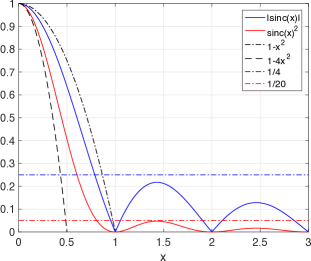
Figure 9: Simple bounds on $|{\rm sinc}(x)|$ and ${\rm sinc}(x)^{2}$.

Concavity of a Special Function

Consider the function

$$f(P)=\left(a+b\sqrt{P}+cP\right)\frac{\sqrt{\pi}}{2}\,\frac{{\rm erf}\left(\sqrt{sP}\right)}{\sqrt{sP}}$$ (295)

where $a$, $b$, and $c$ are non-negative constants and $s$ is a positive constant. We compute

$$\frac{df}{dP}= \frac{e^{-sP}}{2sP^{3/2}}\left[(cP+a)s\sqrt{P}+bsP\right.$$

$$\qquad\left.+\sqrt{s}\,(cP-a)\,e^{sP}\frac{\sqrt{\pi}}{2}{\rm erf}\left(\sqrt{sP}\right)\right]$$ (296)

$$\frac{d^{2}f}{dP^{2}}= -\frac{e^{-sP}}{4P^{2}\sqrt{sP}}\left[\sqrt{s}P\left\{2s\sqrt{P}(cP+a)+2bsP+b\right\}\right.$$

$$\left.+(cP-3a)\left\{e^{sP}\frac{\sqrt{\pi}}{2}{\rm erf}\left(\sqrt{sP}\right)-\sqrt{sP}\right\}\right].$$ (297)

From (296), we see that $f(P)$ is non-decreasing if $cP\geq a$. Similarly, for (297) we use [28, 8.253.1] to bound

$$e^{y^{2}}\cdot\frac{\sqrt{\pi}}{2}{\rm erf}(y)\geq y$$ (298)

for $y\geq 0$ and find that $f(P)$ is concave if $cP\geq 3a$. Thus, $f(P+3a/c)$ is both non-decreasing and concave if $P\geq 0$ and $c>0$.

TABLE II: List of Acronyms, Symbols, and Notation

Acronyms		Defined in:
ASK, FSK, PSK	Amplitude-, frequency-, phase-shift keying	Sec. IV-B and VI-B
AWGN	Additive white Gaussian noise	Sec. I
EDFA	Erbium-doped fiber amplifier	Sec. III-B
LHS, RHS	Left-hand side, right-hand side	Sec. II-E and IV-D
NLSE	Nonlinear Schrödinger equation	Sec. I-A and III-A
OA	Optical amplification / optical amplifier	Sec. I
PAM	Pulse amplitude modulation	Sec. II-C
PDD, PSD, PSDD	Power distance density, power spectral density, power spectral-distance density	Sec. I and III-B
SNR	Signal-to-noise ratio	Sec. II-D
SPM, XPM	Self-phase modulation, cross-phase modulation	Sec. V and V-B
WDM	Wavelength division multiplexing	Sec. I
Fiber and Noise Parameters
$\alpha$, $\beta_{1}$, $\beta_{2}$	Loss coefficient, group velocity, group velocity dispersion	Sec. III-A
$\gamma$	Nonlinear Kerr coefficient	Sec. III-A
$k_{B}$, $T_{e}$	Boltzmann’s constant, temperature	Sec. II-D
$N_{0}=k_{B}T_{e}$	receiver noise PSD	Sec. II-D
$N_{A}$	OA noise PSDD	Sec. III-B
$K=N_{A}B$	OA noise PDD	Sec. III-B
$\rho(t-t^{\prime})$	OA noise correlation coefficient	Sec. III-B
Signal Parameters and Variables
$B$	OA bandwidth	Sec. I-A and III-B
$W$	Signal or receiver bandwidth	Sec. I-A, IV-C and VII-D
$f_{0}$	Carrier frequency	Sec. III-A
$T_{s}$	Time period of PAM	Sec. II-C
$P$, $P_{t}$, $P_{o}$	Average launch power, instantaneous launch power, offset power	Sec. I, VII-A and VII-C
$c$	$-j\gamma(K/2)\sqrt{1-\rho^{2}}$	Sec. II-E and (63)
$\kappa$	$2\gamma^{2}Kz^{3}/3$	Sec. V-A and (73)
$\delta$	Variable used for bounding	Sec. V-B and (82)
$S(c)$, $S_{R}(c)$, $S_{I}(c)$	$\operatorname{sech}\left(\sqrt{2c}\,z\right)$, real part $\Re(S(c))$, imaginary part $\Im(S(c))$	Sec. II-E
$T(c)$, $T_{R}(c)$, $T_{I}(c)$	$\left.\tanh\left(\sqrt{2c}\,z\right)\right/\sqrt{2c}$, real part $\Re(T(c))$, imaginary part $\Im(T(c))$	Sec. II-E
Signals
$u(z,t)=u_{z}(t)=u(t)=u$	Signal at distance $z$ and time $t$	Sec. II-A
$u(z,t^{\prime})=u_{z}(t^{\prime})=u(t^{\prime})=u^{\prime}$	Signal at distance $z$ and time $t^{\prime}$	Sec. II-A
$U(z,t)=U_{z}(t)=U(t)=U$	Random signal at distance $z$ and time $t$	Sec. II-A
$U(z,t^{\prime})=U_{z}(t^{\prime})=U(t^{\prime})=U^{\prime}$	Random signal at distance $z$ and time $t^{\prime}$	Sec. II-A
$\tilde{u}(z,f)$	Fourier transform of $u(z,t)$ at distance $z$	Sec. III-C
$u_{r}(t)$	Receiver signal with AWGN	Sec. II-D
$N_{r}(\cdot)$ and $n_{r}(\cdot)$	Receiver AWGN process and its realization	Sec. II-D
$W(z,t)$, $W_{R}(z,t)$, $W_{I}(z,t)$	Spatial Wiener process, real part $\Re(W(z,t))$, imaginary part $\Im(W(z,t))$	Sec. III-B
$\hat{w}(z,t)$	Accumulated noise for the model (39)	Sec. III-D and (41)
$\left\{\phi_{m}(\cdot)\right\}_{m=1}^{\infty}$	Complete orthonormal basis	Sec. IV-B
$b(t)$ and $\tilde{b}(f)$	$2W\,{\rm sinc}\left(Wt\right)^{2}$ and its Fourier transform	Sec. IV-C
Autocorrelation Functions
$A_{z}(t,t^{\prime})=A(t,t^{\prime})$	Autocorrelation function at distance $z$ conditioned on $U_{0}=u_{0}$	Sec. II-B
$\bar{A}_{z}(t,t^{\prime})=\bar{A}(t,t^{\prime})$	Average autocorrelation function at distance $z$	Sec. II-B
$\bar{A}(\tau)$	Time-averaged autocorrelation function at distance $z$	Sec. II-C
$\mathcal{A}(t,t^{\prime})$	Approximate autocorrelation function at distance $z$ conditioned on $U_{0}=u_{0}$	Sec. V-A
$\bar{\mathcal{A}}(t,t^{\prime})$, $\bar{\mathcal{A}}(\tau)$	Average approximate autocorrelation functions at distance $z$	Sec. VI-B
PSD, Receiver Power, Receiver Energy
$\bar{\mathcal{P}}(f)$, $\bar{\mathcal{P}}(f,T)$	PSDs at distance $z$	Sec. II-B
$\bar{P}_{r}(W)$, $\bar{P}_{r}(W,T)$	Average receiver powers in a band of bandwidth $W$	Sec. II-D and IV-C
$P_{r}(W,T,t)$	Upper bound on instantaneous receiver power conditioned on $U_{0}=u_{0}$	Sec. VII-A
$E_{m}(T_{r})$	Energy at receiver in time interval $[mT_{r},(m+1)T_{r})$ conditioned on $U_{0}=u_{0}$	Sec. IV-D
$\bar{E}_{m}(T_{r})$	Average energy at receiver in time interval $[mT_{r},(m+1)T_{r})$	Sec. IV-D
$E_{m}(T_{r},t)$	Upper bound on instantaneous receiver energy conditioned on $U_{0}=u_{0}$	Sec. VII-F
Capacity
$C(W)$	Capacity with bandwidth $W$	Sec. II-D
$\eta(W)$	Spectral efficiency with bandwidth $W$	Sec. II-D

Gerhard Kramer (S’91-M’94-SM’08-F’10) received the Dr. sc. techn. degree from ETH Zurich in 1998. From 1998 to 2000, he was with Endora Tech AG in Basel, Switzerland, and from 2000 to 2008 he was with the Math Center at Bell Labs in Murray Hill, NJ, USA. He joined the University of Southern California, Los Angeles, CA, USA, as a Professor of Electrical Engineering in 2009. He joined the Technical University of Munich (TUM) in 2010, where he is currently Alexander von Humboldt Professor and Chair of Communications Engineering. His research interests include information theory and communications theory, with applications to wireless, copper, and optical fiber networks. Dr. Kramer served as the 2013 President of the IEEE Information Theory Society.

References

- [1] R. J. Essiambre, G. Kramer, P. J. Winzer, G. J. Foschini, and B. Goebel, “Capacity limits of optical fiber networks,” J. Lightwave Techn., vol. 28, no. 4, pp. 662–701, Feb. 2010.
- [2] A. Mecozzi, “Limits to long-haul coherent transmission set by the Kerr nonlinearity and noise of the in-line amplifiers,” J. Lightwave Techn., vol. 12, no. 11, pp. 1993–2000, Nov. 1994.
- [3] K. S. Turitsyn, S. A. Derevyanko, I. V. Yurkevich, and S. K. Turitsyn, “Information capacity of optical fiber channels with zero average dispersion,” Phys. Rev. Lett., vol. 91, no. 20, pp. 203901(1–4), Nov. 2003.
- [4] M. I. Yousefi and F. R. Kschischang, “On the per-sample capacity of nondispersive optical fibers,” IEEE Trans. Inf. Theory, vol. 57, no. 11, pp. 7522–7541, Nov. 2011.
- [5] A. Mecozzi, “Probability density functions of the nonlinear phase noise,” Opt. Lett., vol. 29, no. 7, pp. 673–675, Apr. 2004.
- [6] I. S. Terekhov, A. V. Reznichenko, Y. A. Kharkov, and S. K. Turitsyn, “Optimal input signal distribution and per-sample mutual information for nondispersive nonlinear optical fiber channel at large SNR,” CoRR, vol. abs/1508.05774, 2016.
- [7] J. Fahs, A. Tchamkerten, and M. I. Yousefi, “Capacity-achieving input distributions in nondispersive optical fibers,” CoRR, vol. abs/1704.04904, 2017.
- [8] J. Tang, “The Shannon channel capacity of dispersion-free nonlinear optical fiber transmission,” J. Lightwave Techn., vol. 19, no. 8, pp. 1104–1109, Aug. 2001.
- [9] J. Tang, “The multispan effects of Kerr nonlinearity and amplifier noises on Shannon channel capacity of a dispersion-free nonlinear optical fiber,” J. Lightwave Techn., vol. 19, no. 8, pp. 1110–1115, Aug 2001.
- [10] M. S. Pinsker, Information and Information Stability of Random Variables and Processes, Holden Day, 1964.
- [11] H. Wei and D. V. Plant, “Comment on ”Information capacity of optical fiber channels with zero average dispersion”,” CoRR, vol. abs/physics/0611190, 2006.
- [12] A. D. Wyner, “The capacity of the band-limited Gaussian channel,” Bell Sys. Tech. J., vol. 45, no. 3, pp. 359–395, Mar. 1966.
- [13] J. G. Proakis and M. Salehi, Digital Communications, McGraw Hill, 5th edition, 2008.
- [14] C. E. Shannon, “A mathematical theory of communication,” Bell Sys. Tech. J., vol. 27, pp. 379–423 and 623–656, July and October 1948, Reprinted in Claude Elwood Shannon: Collected Papers, pp. 5-83, (N.J.A. Sloane and A.D. Wyner, eds.) Piscataway: IEEE Press, 1993.
- [15] M. Gastpar, “On capacity under receive and spatial spectrum-sharing constraints,” IEEE Trans. Inf. Theory, vol. 53, no. 2, pp. 471–487, Feb. 2007.
- [16] G. P. Agrawal, Nonlinear Fiber Optics, Academic Press, 3rd edition, 2001.
- [17] R. G. Gallager, Information Theory and Reliable Communication, Wiley, New York, 1968.
- [18] D. Slepian, “On bandwidth,” Proc. IEEE, vol. 64, pp. 292–300, Mar. 1976.
- [19] B. Goebel, R. J. Essiambre, G. Kramer, P. J. Winzer, and N. Hanik, “Calculation of mutual information for partially coherent Gaussian channels with applications to fiber optics,” IEEE Trans. Inf. Theory, vol. 57, no. 9, pp. 5720–5736, Sept. 2011.
- [20] L. Barletta and G. Kramer, “Signal-to-noise ratio penalties for continuous-time phase noise channels,” in Int. Conf. Cognitive Radio Oriented Wireless Networks Commun., June 2014, pp. 232–235.
- [21] L. Barletta and G. Kramer, “On continuous-time white phase noise channels,” in IEEE Int. Symp. Inf. Theory, Honolulu, HI, June 2014, pp. 2426–2429.
- [22] G. Kramer, M. I. Yousefi, and F. R. Kschischang, “Upper bound on the capacity of a cascade of nonlinear and noisy channels,” in IEEE Inf. Theory Workshop, Apr. 2015, pp. 1–4.
- [23] M. I. Yousefi, G. Kramer, and F. R. Kschischang, “Upper bound on the capacity of the nonlinear Schrödinger channel,” in IEEE Can. Workshop Inf. Theory, July 2015, pp. 22–26.
- [24] C. Headly III and G. P. Agrawal, “Noise characteristics and statistics of picosecond Stokes pulses generated in optical fibers through stimulated Raman scattering,” J. Quant. Electron., vol. 31, no. 11, pp. 2058–2067, Nov. 1995.
- [25] R. H. Cameron and W. T. Martin, “Evaluation of various Wiener integrals by use of certain Sturm-Liouville differential equations,” Bull. Amer. Math. Soc., vol. 51, pp. 73–90, Feb. 1945.
- [26] R. H. Cameron and W. T. Martin, “Transformations of Wiener integrals under a general class of linear transformations,” Trans. Amer. Math. Soc., vol. 58, pp. 184–219, Sept. 1945.
- [27] A. Thangaraj, G. Kramer, and G. Böcherer, “Capacity bounds for discrete-time, amplitude-constrained, additive white Gaussian noise channels,” IEEE Trans. Inf. Theory, vol. 63, 2017.
- [28] I. S. Gradshteyn and I. M. Ryzhik, Table of Integrals, Series, and Products, Academic Press, 7th edition, 2007.