Online Learning with Automata-based Expert Sequences

Abstract

We consider a general framework of online learning with expert advice where regret is defined with respect to sequences of experts accepted by a weighted automaton. Our framework covers several problems previously studied, including competing against $k$-shifting experts. We give a series of algorithms for this problem, including an automata-based algorithm extending weighted-majority and more efficient algorithms based on the notion of failure transitions. We further present efficient algorithms based on an approximation of the competitor automaton, in particular $n$-gram models obtained by minimizing the $\infty$-Rényi divergence, and present an extensive study of the approximation properties of such models. Finally, we also extend our algorithms and results to the framework of sleeping experts.

1 Introduction

Online learning is a general model for sequential prediction. Within that framework, the setting of prediction with expert advice has received widespread attention (Littlestone and Warmuth, 1994; Cesa-Bianchi and Lugosi, 2006; Cesa-Bianchi et al., 2007). In this setting, the algorithm maintains a distribution over a set of experts, or selects an expert from an implicitly maintained distribution. At each round, the loss assigned to each expert is revealed. The algorithm incurs the expected loss over the experts and then updates its distribution on the set of experts. Its objective is to minimize its expected regret, that is the difference between its cumulative loss and that of the best expert in hindsight.

However, this benchmark is only significant when the best expert in hindsight is expected to perform well. When that is not the case, then the learner may still play poorly. As an example, it may be that no single baseball team has performed well over all seasons in the past few years. Instead, different teams may have dominated over different time periods. This has led to a definition of regret against the best sequence of experts with $k$ shifts in the seminal work of Herbster and Warmuth (1998) on tracking the best expert. The authors showed that there exists an efficient online learning algorithm for this setting with favorable regret guarantees.

This work has subsequently been improved to account for broader expert classes (Gyorgy et al., 2012), to deal with unknown parameters (Monteleoni and Jaakkola, 2003), and has been further generalized (Cesa-Bianchi et al., 2012; Vovk, 1999). Another approach for handling dynamic environments has consisted of designing algorithms that guarantee small regret over any subinterval during the course of play. This notion, coined as adaptive regret by Hazan and Seshadhri (2009), has been subsequently strengthened and generalized (Daniely et al., 2015; Adamskiy et al., 2012). Remarkably, it was shown by Adamskiy et al. (2012) that the algorithm designed by Herbster and Warmuth (1998) is also optimal for adaptive regret. Koolen and de Rooij (2013) described a Bayesian framework for online learning where the learner samples from a distribution of expert sequences and predicts according to the prediction of that expert sequence. They showed how the algorithms designed for $k$-shifting regret, e.g. (Herbster and Warmuth, 1998; Monteleoni and Jaakkola, 2003), can be interpreted as specific priors in this formulation. There has also been work deriving guarantees in the bandit setting when the losses are stochastic (Besbes et al., 2014; Wei et al., 2016).

(i)	(ii)	(iii)

Figure 1: WFAs representing sequences of experts in $\Sigma=\{a,b,c\}$. (i) $\mathscr{C}_{\text{$k$-shift}}$ with $k=2$ shifts, all weights are equal to one and not indicated; (ii) $\mathscr{C}_{\text{weighted-shift}}$ with $\alpha,\beta,\gamma\in[0,1]$; (iii) $\mathscr{C}_{\text{hierarchy}}$ a hierarchical family of expert sequences: the learner must select expert $a$ from the start, can only shift onto $b$ once, and can only shift onto $c$ twice.

The general problem of online convex optimization in the presence of non-stationary environments has also been studied by many researchers. One perspective has been the design of algorithms that maintain a guarantee against sequences that do not vary too much (Mokhtari et al., 2016; Shahrampour and Jadbabaie, 2016; Jadbabaie et al., 2015; Besbes et al., 2015). Another assumes that the learner has access to a dynamical model that is able to capture the benchmark sequence (Hall and Willett, 2013). György and Szepesvári (2016) reinterpreted the framework of Hall and Willett (2013) to recover and extend the results of Herbster and Warmuth (1998).

In this paper, we generalize the framework just described to the case where the learner’s cumulative loss is compared to that of sequences accepted by a weighted finite automaton (WFA). This strictly generalizes the notion of $k$-shifting regret, since $k$-shifting sequences can be represented by an automaton (see Figure 1), and further extends it to a notion of weighted regret which takes into consideration the sequence weights. Our framework covers a very rich class of competitor classes, including WFAs learned from past observations.

Our contributions are mainly algorithmic but also include several theoretical results and guarantees. We first describe an efficient online algorithm using automata operations that achieves both favorable weighted regret and unweighted regret (Section 3). Next, we present and analyze more efficient solutions based on an approximation of the WFA representing the set of competitor sequences (Section 4), including a specific analysis of approximations via $n$-gram models both when minimizing the $\infty$-Rényi divergence and the relative entropy. Finally, we extend the results above to the sleeping expert setting (Freund et al., 1997), where the learner may not have access to advice from every expert at each round (Section 5).

2 Learning setup

We consider the setting of prediction with expert advice over $T\in\mathbb{N}$ rounds. Let $\Sigma=\{a_{1},\ldots,a_{N}\}$ denote a set of $N$ experts. At each round $t\in[T]$, an algorithm $\mathcal{A}$ specifies a probability distribution ${\mathsf{p}}_{t}$ over $\Sigma$, samples an expert $i_{t}$ from ${\mathsf{p}}_{t}$, receives the vector of losses of all experts ${\mathbf{l}}_{t}\in[0,1]^{N}$, and incurs the specific loss $l_{t}[i_{t}]$. A commonly adopted goal for the algorithm is to minimize its static (expected) regret $\mathrm{Reg}_{T}(\mathcal{A},\Sigma)$, that is the difference between its cumulative expected loss and that of the best expert in hindsight:

$$\mathrm{Reg}_{T}(\mathcal{A},\Sigma)=\max_{x\in\Sigma}\sum_{t=1}^{T}{\mathsf{p}}_{t}\cdot{\mathbf{l}}_{t}-\sum_{t=1}^{T}l_{t}[x].$$ (1)

Here, we will consider an alternative benchmark, typically more demanding, where the cumulative loss of the algorithm is compared against the loss of the best sequence of experts ${\mathbf{x}}\in\Sigma^{T}$ among those accepted by a weighted finite automaton (WFA) $\mathscr{C}$ over the semiring $(\mathbb{R}_{+}\cup\{+\infty\},+,\times,0,1)$. The sequences ${\mathbf{x}}$ accepted by $\mathscr{C}$ are those which are assigned a positive value by $\mathscr{C}$, $\mathscr{C}({\mathbf{x}})>0$, which we will assume to be non-empty. We will denote by $K\geq 1$ the cardinality of that set.

We will take into account the probability distribution ${\mathsf{q}}$ defined by the weights assigned by $\mathscr{C}$ to sequences of length $T$: ${\mathsf{q}}({\mathbf{x}})=\frac{\mathscr{C}({\mathbf{x}})}{\sum_{{\mathbf{x}}\in\Sigma^{T}}\mathscr{C}({\mathbf{x}})}$. This leads to the following definition of weighted regret at time $T$ given a WFA $\mathscr{C}$:

$$\mathrm{Reg}_{T}(\mathcal{A},\mathscr{C})$$ (2)

$$=\max_{\begin{subarray}{c}{\mathbf{x}}\in\Sigma^{T}\\ \mathscr{C}({\mathbf{x}})>0\end{subarray}}\Bigg{\{}\sum_{t=1}^{T}{\mathsf{p}}_{t}\cdot{\mathbf{l}}_{t}-\sum_{t=1}^{T}l_{t}[{\mathbf{x}}[t]]+\log[{\mathsf{q}}({\mathbf{x}})K]\Bigg{\}},$$

where ${\mathbf{x}}[t]$ denotes the $t$th symbol of ${\mathbf{x}}$. The presence of the factor $K$ only affects the regret definition by a constant additive term $\log K$ and is only intended to make the last term vanish when the probability distribution ${\mathsf{q}}$ is uniform, i.e. ${\mathsf{q}}({\mathbf{x}})=\frac{1}{K}$ for all ${\mathbf{x}}$. The last term in the weighted regret definition can be interpreted as follows: for a given value of an expert sequence loss $\sum_{t=1}^{T}l_{t}[{\mathbf{x}}[t]]$, the regret is larger for sequences ${\mathbf{x}}$ with a larger probability ${\mathsf{q}}({\mathbf{x}})$. Thus, with this definition of regret, the learning algorithm is pressed to achieve a small cumulative loss compared to expert sequences with small loss and high probability. Notice that when $\mathscr{C}$ accepts only constant sequences, that is sequences ${\mathbf{x}}$ with ${\mathbf{x}}[1]=\ldots={\mathbf{x}}[T]$ and assigns the same weight to them, then the notion of weighted regret coincides with that of static regret (Formula 1).

We also define the unweighted regret $\mathrm{Reg}_{T}^{0}(\mathcal{A},\mathscr{C})$ of algorithm $\mathcal{A}$ at time $T$ given the WFA $\mathscr{C}$ as:

$$\mathrm{Reg}_{T}^{0}(\mathcal{A},\mathscr{C})=\max_{\begin{subarray}{c}{\mathbf{x}}\in\Sigma^{T}\\ \mathscr{C}({\mathbf{x}})>0\end{subarray}}\Bigg{\{}\sum_{t=1}^{T}{\mathsf{p}}_{t}\cdot{\mathbf{l}}_{t}-\sum_{t=1}^{T}l_{t}[{\mathbf{x}}[t]]\Bigg{\}}.$$ (3)

The weights of the WFA $\mathscr{C}$ play no role in this notion of regret. When $\mathscr{C}$ has uniform weights, then the unweighted regret and weighted regret coincide.

As an example, the sequences of experts with $k$ shifts studied by Herbster and Warmuth (1998) can be represented by the WFA $\mathscr{C}_{\text{$k$-shift}}$ of Figure 1(i). Figure 1(ii) shows an alternative weighted model of shifting experts, and Figure 1(iii) shows a hierarchical family of expert sequences.

3 Automata Weighted-Majority algorithm

In this section, we describe a simple algorithm, Automata Weighted-Majority (AWM), that can be viewed as an enhancement of the weighted-majority algorithm (Littlestone and Warmuth, 1994) to the setting of experts paths represented by a WFA. We will show that it benefits from favorable weighted and unweighted regret guarantees.

As with standard weighted-majority, AWM maintains a distribution ${\mathsf{q}}_{t}$ over the set of expert sequences ${\mathbf{x}}\in\Sigma^{T}$ accepted by $\mathscr{C}$ at any time $t$ and admits a learning parameter $\eta>0$. The initial distribution ${\mathsf{q}}_{1}$ is defined in terms of the distribution ${\mathsf{q}}$ induced by $\mathscr{C}$ over $\Sigma^{T}$, and ${\mathsf{q}}_{t+1}$ is defined from ${\mathsf{q}}_{t}$ via an exponential update: for all ${\mathbf{x}}\in\Sigma^{T},t\geq 1$,

$${\mathsf{q}}_{1}[{\mathbf{x}}]=\frac{{\mathsf{q}}[{\mathbf{x}}]^{\eta}}{\sum_{{\mathbf{x}}\in\Sigma^{T}}{\mathsf{q}}[{\mathbf{x}}]^{\eta}},$$

$${\mathsf{q}}_{t+1}[{\mathbf{x}}]=\frac{e^{-\eta\,l_{t}[{\mathbf{x}}[t]]}{\mathsf{q}}_{t}[{\mathbf{x}}]}{\sum_{{\mathbf{x}}\in\Sigma^{T}}e^{-\eta\,l_{t}[{\mathbf{x}}[t]]}{\mathsf{q}}_{t}[{\mathbf{x}}]},$$ (4)

where we denote by ${\mathbf{x}}[t]\in\Sigma$ the $t$th symbol in ${\mathbf{x}}$. ${\mathsf{q}}_{t}$ induces a distribution ${\mathsf{p}}_{t}$ over the expert set $\Sigma$ defined for all $a\in\Sigma$ by

$${\mathsf{p}}_{t}[a]=\frac{\sum_{{\mathbf{x}}\in\Sigma^{T}}{\mathsf{q}}_{t}[{\mathbf{x}}]1_{{\mathbf{x}}[t]=a}}{\sum_{a\in\Sigma}\sum_{{\mathbf{x}}\in\Sigma^{T}}{\mathsf{q}}_{t}[{\mathbf{x}}]1_{{\mathbf{x}}[t]=a}}.$$ (5)

Thus, ${\mathsf{p}}_{t}[a]$ is obtained by summing up the ${\mathsf{q}}_{t}$-weights of all sequences with the $t$th symbol equal to $a$ and normalization. The distributions ${\mathsf{p}}_{t}$ define the AWM algorithm. Note that the algorithm cannot be viewed as weighted-majority with ${\mathsf{q}}$-priors on expert sequences as ${\mathsf{q}}_{1}$ is defined in terms of ${\mathsf{q}}^{\eta}$.

The following regret guarantees hold for AWM.

Theorem 1.

Let ${\mathsf{q}}$ denote the probability distribution over expert sequences of length $T$ defined by $\mathscr{C}$ and let $K$ denote the cardinality of its support. Then, the following upper bound holds for the weighted regret of AWM:

$$\mathrm{Reg}_{T}(\textsc{AWM},\mathscr{C}) \leq\frac{\eta T}{8}+\frac{1}{\eta}\log\bigg{[}K^{\eta}\sum_{{\mathbf{x}}\in\Sigma^{T}}{\mathsf{q}}[{\mathbf{x}}]^{\eta}\bigg{]}$$

$$\leq\frac{\eta T}{8}+\frac{1}{\eta}\log K.$$

Furthermore, when $K\geq 2$, for any $T>0$, there exists $\eta^{*}>0$, decreasing as a function of $T$, such that:

$$\mathrm{Reg}_{T}(\textsc{AWM},\mathscr{C}) \leq\sqrt{\frac{TH_{\eta^{*}}({\mathsf{q}})}{2}}-H_{\eta^{*}}({\mathsf{q}})+\log K,$$

where $H_{\eta}({\mathsf{q}})=\frac{1}{1-\eta}\log\left(\sum_{{\mathbf{x}}\in\Sigma^{T}}{\mathsf{q}}[{\mathbf{x}}]^{\eta}\right)$ is the $\eta$-Rényi entropy of ${\mathsf{q}}$. The unweighted regret of AWM can be upper-bounded as follows:

$$\mathrm{Reg}_{T}^{0}(\textsc{AWM},\mathscr{C}) \leq\frac{\eta T}{8}+\frac{1}{\eta}\log K.$$

The proof is an extension of the standard proof for the weighted-majority algorithm and is given in Appendix C. The bound in terms of the Rényi entropy shows that the regret guarantee can be substantially more favorable than standard bounds of the form $O(\sqrt{T\log K})$, depending on the properties of the distribution ${\mathsf{q}}$. First, since the $\eta$-Rényi entropy is non-increasing in $\eta$ (Van Erven and Harremos, 2014), we have $H_{\eta^{*}}({\mathsf{q}})\leq H_{0}({\mathsf{q}})=\log(|\operatorname*{supp}({\mathsf{q}})|)\leq\log K$. Second, if the distribution ${\mathsf{q}}$ is concentrated on a subset $\Delta$ with a small cardinality, $|\Delta|\ll K$, that is $\sum_{{\mathbf{x}}\not\in\Delta}{\mathsf{q}}[{\mathbf{x}}]^{\eta^{*}}<\epsilon(1-\eta^{*})\sum_{{\mathbf{x}}\in\Delta}{\mathsf{q}}[{\mathbf{x}}]^{\eta^{*}}$ for some $\epsilon>0$ and for $\eta^{*}<1$, then, by Jensen’s inequality, the following upper bound holds:

$$H_{\eta}^{*}({\mathsf{q}}) \leq\frac{1}{1-\eta^{*}}\log\bigg{(}\sum_{{\mathbf{x}}\in\Delta}{\mathsf{q}}[{\mathbf{x}}]^{\eta^{*}\!}\bigg{)}+\epsilon$$

$$\leq\frac{1}{1-\eta^{*}}\log\bigg{(}|\Delta|\bigg{(}\frac{1}{|\Delta|}\sum_{{\mathbf{x}}\in\Delta}{\mathsf{q}}[{\mathbf{x}}]\bigg{)}^{\eta^{*}\!}\bigg{)}+\epsilon$$

$$\leq\log(|\Delta|)+\epsilon.$$

Efficient algorithm. We now present an efficient computation of the distributions ${\mathsf{p}}_{t}$. Algorithm 1 gives the pseudocode of our algorithm. We will assume throughout that $\mathscr{C}$ is deterministic, that is it admits a single initial state and no two transitions leaving the same state share the same label. We can efficiently compute a WFA accepting the set of sequences of length $T$ accepted by $\mathscr{C}$ by using the standard intersection algorithm for WFAs (see Appendix A for more detail on this algorithm). Let $\mathscr{S}_{T}$ be a deterministic WFA accepting the set of sequences of length $T$ and assigning weight one to each (see Figure 3). Then, the intersection of $\mathscr{C}$ and $\mathscr{S}_{T}$ is a WFA denoted by $\mathscr{C}\cap\mathscr{S}_{T}$ which, by definition, assigns to each sequence ${\mathbf{x}}\in\Sigma^{T}$ the weight

$$(\mathscr{C}\cap\mathscr{S}_{T})({\mathbf{x}})=\mathscr{C}({\mathbf{x}})\times\mathscr{S}_{T}({\mathbf{x}})=\mathscr{C}({\mathbf{x}}),$$ (6)

and assigns weight zero to all other sequences. Furthermore, the WFA $\mathscr{B}=(\mathscr{C}\cap\mathscr{S}_{T})$ returned by the intersection algorithm is deterministic since both $\mathscr{C}$ and $\mathscr{S}_{T}$ are deterministic. Next, we replace each transition weight of $\mathscr{B}$ by its $\eta$-power. Since $\mathscr{B}$ is deterministic, this results in a WFA that we denote by $\mathscr{B}^{\eta}$ and that associates to each sequence ${\mathbf{x}}$ the weight $\mathscr{C}[{\mathbf{x}}]^{\eta}$. Normalizing $\mathscr{B}^{\eta}$ results in a WFA $\mathscr{A}$ assigning weight $\mathscr{A}[{\mathbf{x}}]=\frac{\mathscr{B}[{\mathbf{x}}]^{\eta}}{\sum_{x}\mathscr{B}[{\mathbf{x}}]^{\eta}}={\mathsf{q}}_{1}[x]$ to any ${\mathbf{x}}\in\Sigma^{T}$. This normalization can be achieved in time that is linear in the size of the WFA $\mathscr{B}^{\eta}$ using the Weight-Pushing algorithm (Mohri, 1997, 2009). For completeness, we describe this algorithm in Appendix B. Note that since $\mathscr{B}^{\eta}$ is acyclic, its size is in $O(|E_{\mathscr{A}}|)$. We will denote by $\mathscr{A}$ the resulting WFA.

For any state $u$ of $\mathscr{A}$, we will denote by ${\boldsymbol{\beta}}[u]$ the sum of the weights of all paths from $u$ to a final state. The vector ${\boldsymbol{\beta}}$ can be computed in time that is linear in the number of states and transitions of $\mathscr{A}$ using a simple single-source shortest-distance algorithm in the semiring $(\mathbb{R}_{+}\cup\{+\infty\},+,\times,0,1)$ (Mohri, 2009), or the forward-backward algorithm. We call this subroutine BwdDist in the pseudocode.

Algorithm:  AWM($\mathscr{C}$, $\eta$)

$\mathscr{B}\leftarrow\mathscr{C}\cap\mathscr{S}_{T}$

$\mathscr{A}\leftarrow\textsc{Weight-Pushing}(\mathscr{B}^{\eta})$

${\boldsymbol{\beta}}\leftarrow\textsc{BwdDist}(\mathscr{A})$

${\boldsymbol{\alpha}}\leftarrow 0$; ${\boldsymbol{\alpha}}[I_{\mathscr{A}}]\leftarrow 1$

for each $e\in E_{\mathscr{A}}^{0\to 1}$ do

      ${\mathsf{p}}_{1}[\mathrm{lab}[e]]\leftarrow\mathrm{weight}[e]$.

      for $t\leftarrow 1$ to $T$ do

           $i_{t}\leftarrow$Sample(${\mathsf{p}}_{t}$); Play($i_{t}$); Receive(${\mathbf{l}}_{t}$)

           $Z\leftarrow 0$; ${\mathbf{w}}\leftarrow 0$

           for each $e\in E_{\mathscr{A}}^{t\to t+1}$ do

                $\mathrm{weight}[e]\leftarrow\mathrm{weight}[e]\,e^{-\eta l_{t}[\mathrm{lab}[e]]}$

                ${\mathbf{w}}[\mathrm{lab}[e]]\leftarrow{\mathbf{w}}[\mathrm{lab}[e]]+{\boldsymbol{\alpha}}[\mathrm{src}[e]]\,\mathrm{weight}[e]\,{\boldsymbol{\beta}}[\mathrm{dest}[e]]$

                $Z\leftarrow Z+{\mathbf{w}}[\mathrm{lab}[e]]$

                ${\boldsymbol{\alpha}}[\mathrm{dest}[e]]\leftarrow{\boldsymbol{\alpha}}[\mathrm{dest}[e]]+{\boldsymbol{\alpha}}[\mathrm{src}[e]]\,\mathrm{weight}[e]$

                ${\mathsf{p}}_{t+1}\leftarrow\frac{{\mathbf{w}}}{Z}$

               

Algorithm 1 AutomataWeightedMajority(AWM).

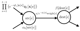
Figure 2: WFA $\mathscr{S}_{T}$, for $\Sigma=\{a,b,c\}$ and $T=3$.

Figure 3: Illustration of algorithm AWM.

We will denote by $Q_{t}$ the set of states in $\mathscr{A}$ that can be reached by sequences of length $t$ and by $E_{\mathscr{A}}^{t\to t+1}$ the set of transitions from a state in $Q_{t}$ to a state in $Q_{t+1}$. For each transition $e$, let $\mathrm{src}[e]$ denote its source state, $\mathrm{dest}[e]$ its destination state, $\mathrm{lab}[e]\in\Sigma$ its label, and $\mathrm{weight}[e]\geq 0$ its weight. Since $\mathscr{A}$ is normalized, the expert probabilities ${\mathsf{p}}_{1}[a]$ for $a\in\Sigma$ can be read off the transitions leaving the initial state: ${\mathsf{p}}_{1}[a]$ is the weight of the transition in $E_{\mathscr{A}}^{0\to 1}$ labeled with $a$.

Let ${\boldsymbol{\alpha}}_{t}[u]$ denote the forward weights, that is the sum of the weights of all paths from the initial state to state $u$ just before the $t$th round. At round $t$, the weight of each transition $e$ in $E_{\mathscr{A}}^{t\to t+1}$ is multiplied by $e^{-\eta l_{t}[\mathrm{lab}[e]]}$. This results in new forward weights ${\boldsymbol{\alpha}}_{t+1}[u]$ at the end of the $t$-th iteration. ${\boldsymbol{\alpha}}_{t+1}$ can be straightforwardly derived from ${\boldsymbol{\alpha}}_{t}$ since for $u\in Q_{t+1}$, ${\boldsymbol{\alpha}}_{t+1}[u]$ is given by ${\boldsymbol{\alpha}}_{t+1}[u]=\sum_{e\colon\mathrm{dest}[e]=u}{\boldsymbol{\alpha}}_{t}[\mathrm{src}[e]]\mathrm{weight}[e]$.

Observe that for any $t\in[T]$ and ${\mathbf{x}}$, ${\mathsf{q}}_{t}[{\mathbf{x}}]$ can be written as follows by unwrapping its recursive update definition:

$${\mathsf{q}}_{t}[{\mathbf{x}}]=\frac{e^{-\eta\sum_{s=1}^{t-1}l_{s}[{\mathbf{x}}[s]]}{\mathsf{q}}_{1}[{\mathbf{x}}]}{\sum_{{\mathbf{x}}\in\Sigma^{T}}e^{-\eta\sum_{s=1}^{t-1}l_{s}[{\mathbf{x}}[s]]}{\mathsf{q}}_{1}[{\mathbf{x}}]}.$$

In view of that, for any $a\in\Sigma$, ${\mathsf{p}}_{t+1}[a]$ can be written as follows:

$${\mathsf{p}}_{t+1}[a] =\frac{\sum_{{\mathbf{x}}\in\Sigma^{T}}e^{-\eta\sum_{s=1}^{t}l_{s}[{\mathbf{x}}[s]]}{\mathsf{q}}_{1}[{\mathbf{x}}]1_{{\mathbf{x}}[t]=a}}{\sum_{a\in\Sigma}\sum_{{\mathbf{x}}\in\Sigma^{T}}e^{-\eta\sum_{s=1}^{t}l_{s}[{\mathbf{x}}[s]]}{\mathsf{q}}_{1}[{\mathbf{x}}]1_{{\mathbf{x}}[t]=a}}.$$

Since the WFA $\mathscr{A}$ is deterministic, for any ${\mathbf{x}}$ accepted by $\mathscr{A}$ there is a unique accepting path $\pi$ in $\mathscr{A}$ labeled with ${\mathbf{x}}$. The numerator of the expression of ${\mathsf{p}}_{t+1}[a]$ is then the sum of the weights of all paths in $\mathscr{A}$ with the $t$th symbol $a$ at the end of $t$th iteration. This can be expressed as the sum over all transitions $e$ in $E_{\mathscr{A}}^{t\to t+1}$ with label $a$ of the total flow through $e$, that is the sum of the weights of all accepting path going through $e$: ${\boldsymbol{\alpha}}_{t}[\mathrm{src}[e]]\,\mathrm{weight}[e]\,{\boldsymbol{\beta}}[\mathrm{dest}[e]]$ (see Figure 3). This is precisely the formula determining ${\mathsf{p}}_{t+1}$ in the pseudocode, where $Z$ is the normalization factor.

The AWM algorithm is closely related to the Expert Hidden Markov Model of Koolen and de Rooij (2013) given for the log loss. It can be viewed as a generalization of that algorithm to arbitrary loss functions. A key difference between our setup and the perspective adopted by Koolen and de Rooij (2013) is that they assume a Bayesian setting where a prior distribution over expert sequences is given and must be used. We assume the existence of a competitor automaton $\mathscr{C}$, but do not necessarily need to sample from it for making predictions. This will be crucial in the next section, where we use a different WFA than $\mathscr{C}$ to improve computational efficiency while preserving regret performance. Also, the prior distribution in (Koolen and de Rooij, 2013) would be over $\mathscr{C}_{T}$ (for a large $T$) and not $\mathscr{C}$.

The computational complexity of AWM at each round $t$ is $O\big{(}|E_{\mathscr{A}}^{t\to t+1}|\big{)}$, that is the time to update the weights of the transitions in $E_{\mathscr{A}}^{t\to t+1}$ and to incrementally compute ${\boldsymbol{\alpha}}$ for states reached by paths of length $t+1$. The total computational cost of the algorithm is thus $O\big{(}\sum_{t=1}^{T}|E_{\mathscr{A}}^{t\to t+1}|\big{)}=O(|E_{\mathscr{A}}|)$, where $E_{\mathscr{A}}$ is the set of transitions of $\mathscr{A}$. Note that $\mathscr{A}$ and $\mathscr{C}\cap\mathscr{S}_{T}$ admit the same topology, thus the total complexity of the algorithm depends on the number of transitions of the intersection WFA $\mathscr{C}\cap\mathscr{S}_{T}$, which is at most $|\mathscr{C}|NT$. This can be substantially more favorable than a naïve algorithm, whose worst-case complexity is exponential in $T$.

When the number of transitions of the intersection WFA $\mathscr{C}\cap\mathscr{S}_{T}$ is not too large compared to the number of experts $N$, the AWM algorithm is quite efficient. However, it is natural to ask whether one can design efficient algorithms even if the number of transitions $E_{\mathscr{A}}^{t\to t+1}$ to process per round is large (which may be the case even for a minimized WFA $\mathscr{C}\cap\mathscr{S}_{T}$ (Mohri, 2009)).

We will give two sets of solutions to derive a more efficient algorithm, which can be combined for further efficiency. In the next section, we discuss a solution that consists of using an approximate WFA with a smaller number of transitions. In Appendix E, we show that the notion of failure transition, originally used in the design of string-matching algorithms and recently employed for parameter estimation in backoff $n$-gram language models (Roark et al., 2013), can be used to derive a more compact representation of the WFA $\mathscr{C}\cap\mathscr{S}_{T}$, thereby resulting in a significantly more efficient online learning algorithm that still admits compelling regret guarantees.

4 Approximation algorithms

In this section, we present approximation algorithms for the problem of online learning against a weighted sequence of experts represented by a WFA $\mathscr{C}$. Rather than using the intersection WFA $\mathscr{C}_{T}=\mathscr{C}\cap\mathscr{S}_{T}$, we will assume that AWM is run with an approximate WFA $\widehat{\mathscr{C}}_{T}$. The main motivation for doing so is that the algorithm can be substantially more efficient if $\widehat{\mathscr{C}}_{T}$ admits significantly fewer transitions than $\mathscr{C}_{T}$. Of course, this comes at the price of a somewhat weaker regret guarantee that we now analyze in detail.

4.1 Effect of WFA approximation

We first analyze the effect of automata approximation on the regret of AWM. As in the previous section, we denote by ${\mathsf{q}}$ the distribution defined by $\mathscr{C}_{T}$ over sequences of length $T$. We will similarly denote by $\widehat{\mathsf{q}}$ the distribution defined by $\widehat{\mathscr{C}}_{T}$ over the same set. The effect of the WFA approximation on the regret can be naturally expressed in terms of the $\infty$-Rényi divergence $D_{\infty}({\mathsf{q}}\|\widehat{\mathsf{q}})$ between the distributions ${\mathsf{q}}$ and $\widehat{\mathsf{q}}$, which is defined by $D_{\infty}({\mathsf{q}}\|\widehat{\mathsf{q}})=\sup_{{\mathbf{x}}\in\Sigma^{T}}\log[{\mathsf{q}}({\mathbf{x}})/\widehat{\mathsf{q}}({\mathbf{x}})]$.

Theorem 2.

The weighted regret of the AWM algorithm with respect to the WFA $\mathscr{C}$ when run with $\widehat{\mathscr{C}}_{T}$ instead of $\mathscr{C}_{T}$ can be upper bounded as follows:

$$\mathrm{Reg}_{T}(\mathcal{A},\mathscr{C}) \leq\frac{\eta T}{8}+\frac{1}{\eta}\log\Big{[}K^{\eta}\sum_{{\mathbf{x}}}\widehat{\mathsf{q}}[{\mathbf{x}}]^{\eta}\Big{]}+D_{\infty}({\mathsf{q}}\|\widehat{\mathsf{q}})$$

$$\leq\frac{\eta T}{8}+\frac{1}{\eta}\log K+D_{\infty}({\mathsf{q}}\|\widehat{\mathsf{q}}).$$

Its unweighted regret can be upper bounded as follows:

$$\mathrm{Reg}_{T}^{0}(\mathcal{A},\mathscr{C}) \leq\max_{\mathscr{C}({\mathbf{x}})>0}\frac{\eta T}{8}+\frac{1}{\eta}\log\bigg{[}\frac{1}{{\mathsf{q}}[{\mathbf{x}}]}\bigg{]}+\frac{1}{\eta}D_{\infty}({\mathsf{q}}\|\widehat{\mathsf{q}}).$$

The proof is given in Appendix D. Theorem 2 shows that the extra cost of using an approximate WFA $\widehat{\mathscr{C}}_{T}$ instead of $\mathscr{C}_{T}$ is $D_{\infty}({\mathsf{q}}\|\widehat{\mathsf{q}})$ for the weighted regret and similarly $\frac{1}{\eta}D_{\infty}({\mathsf{q}}\|\widehat{\mathsf{q}})$ for the unweighted regret. The bound is tight since the best sequence in hindsight in the regret definition may also be the one maximizing the log-ratio.

The theorem suggests a general algorithm for selecting an approximate WFA $\widehat{\mathscr{C}}$ out of a family $\mathcal{C}$ of WFAs with a relatively small number of transitions. This consists of choosing $\widehat{\mathscr{C}}$ to minimize the Rényi divergence as defined by the following program:

$$\min_{\widehat{\mathscr{C}}\in\mathcal{C}}D_{\infty}({\mathsf{q}}\|\widehat{\mathsf{q}}),$$ (7)

where $\widehat{q}$ is the distribution induced by $\widehat{\mathscr{C}}$ over $\Sigma^{T}$ (the one obtained by computing $\widehat{\mathscr{C}}_{T}=\widehat{\mathscr{C}}\cap\mathscr{S}_{T}$ and normalizing the weights). The theorem ensures that the solution benefits from the most favorable regret guarantee among the WFAs in $\mathcal{C}$. When the set of distributions associated to $\mathcal{C}$ is convex, then the set of distributions defined over $\Sigma^{T}$ is also convex. This is then a convex optimization problem, since $\widehat{\mathsf{q}}\mapsto\log({\mathsf{q}}/\widehat{\mathsf{q}})$ is a convex function and the supremum of convex functions is convex.

The choice of the family $\mathcal{C}$ is subject to a trade-off: approximation accuracy versus computational efficiency of using WFAs in $\mathcal{C}$. This raises a model selection question for which we discuss in detail a solution in Section 4.2: given a sequence of families $(\mathcal{C}_{n})_{n\in{\mathbf{N}}}$ with growing complexity and computational cost, the problem consists of selecting the best $n$.

In the following, we will consider the case where the family $\mathcal{C}$ of weighted automata is that of $n$-gram models, for which we can upper bound the computational complexity.

4.2 Minimum Rényi divergence $n$-gram models

Let $\Sigma^{\leq n-1}$ denote the set of sequences of length at most $n-1$. An $n$-gram language model is a Markovian model of order $(n-1)$ defined over $\Sigma^{*}$, which can be compactly represented by a WFA with each state identified with a sequence ${\mathbf{x}}\in\Sigma^{\leq n-1}$, thereby encoding the sequence just read to reach that state. The WFA admits a transition from state $({\mathbf{x}}[1]\cdots{\mathbf{x}}[n-1])$ to state $({\mathbf{x}}[2]\cdots{\mathbf{x}}[n-1]a)$ with weight ${\mathsf{w}}\big{[}a\,|\,{\mathbf{x}}[1]\cdots{\mathbf{x}}[n-1]\big{]}$, for any $a\in\Sigma$, and, for any $k\leq n-1$, a transition from state $({\mathbf{x}}[1]\cdots{\mathbf{x}}[k-1])$ to state $({\mathbf{x}}[1]\cdots{\mathbf{x}}[k-1]a)$ with weight ${\mathsf{w}}\big{[}a\,|\,{\mathbf{x}}[1]\cdots{\mathbf{x}}[k-1]\big{]}$, for any $a\in\Sigma$. It admits a unique initial state which is the one labeled with the empty string $\epsilon$ (sequence of length zero) and all its states are final. The WFA is stochastic, that is outgoing transition weights sum to one at every state: thus, $\sum_{a\in\Sigma}{\mathsf{w}}[a|{\mathbf{x}}]=1$ for all ${\mathbf{x}}\in\Sigma^{\leq n-1}$. Notice that this WFA is also deterministic since it admits a unique initial state and no two transitions with the same label leaving any state. Figure 4 illustrates this definition in the case of a simple bigram model.

Note that the transition weights ${\mathsf{w}}[a|{\mathbf{x}}]$, with $a\in\Sigma$ and ${\mathbf{x}}\in\cup_{k\leq n-1}\Sigma^{k}$ fully specify an $n$-gram model. Since for a fixed ${\mathbf{x}}\in\cup_{k\leq n-1}\Sigma^{k}$, ${\mathsf{w}}[\cdot|{\mathbf{x}}]$ is an element of the simplex, an $n$-gram model can be viewed as an element of the product of $\sum_{k=0}^{n-1}\Sigma^{k}$ simplices, a convex set. We will denote by $\mathcal{W}_{n}$ the family of all $n$-gram models.

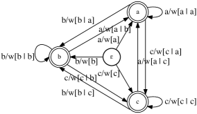
Figure 4: A bigram language model over the alphabet $\Sigma=\{a,b,c\}$.

One key advantage of $n$-gram models in this context is that the per-iteration complexity can be bounded in terms of the number of symbols. Since an $n$-gram model has at most $|\Sigma|^{n-1}$ states, its per-iteration computational cost is in $O\big{(}|\Sigma|^{n}\big{)}$ as each state can take one of $|\Sigma|$ possible transitions. For $n$ small, this can be very advantageous compared to the original $\mathscr{C}_{T}$, since in general the maximum out-degree of states reached by sequences of length $t$ in the latter can be very large. For instance, the automaton $\mathscr{C}_{\text{weighted-shift}}$ in Figure 1 (ii) can itself be viewed as a bigram model and admits efficient computation.

For $n$-gram models, our approximation algorithm (Problem 7) can be written as follows:

$$\min_{{\mathsf{w}}\in\mathcal{W}_{n}}D_{\infty}({\mathsf{q}}\|{\mathsf{q}}_{{\mathsf{w}}})=\min_{{\mathsf{w}}\in\mathcal{W}_{n}}\sup_{{\mathbf{x}}\in\Sigma^{T}}\log\bigg{[}\frac{{\mathsf{q}}[{\mathbf{x}}]}{{\mathsf{q}}_{{\mathsf{w}}}[{\mathbf{x}}]}\bigg{]},$$ (8)

where ${\mathsf{q}}_{{\mathsf{w}}}$ is the distribution induced by the $n$-gram model ${\mathsf{w}}$ on sequences in $\Sigma^{T}$. By definition of the $n$-gram model, for any ${\mathbf{x}}\in\Sigma^{T}$, ${\mathsf{q}}_{{\mathsf{w}}}[{\mathbf{x}}]$ is given by the following:

$${\mathsf{q}}_{{\mathsf{w}}}[{\mathbf{x}}]=\prod_{t=1}^{T}{\mathsf{w}}\big{[}{\mathbf{x}}[t]\big{|}{\mathbf{x}}_{\max(t-n+1,1)}^{t-1}\big{]},$$

since the weights of sequences of any fixed length sum to one in an $n$-gram model. Problem 8 is a convex optimization problem over $\mathcal{W}_{n}$. The problem can be solved using as an an extension of the Exponentiated Gradient (EG) algorithm of Kivinen and Warmuth (1997), which we will refer to as Prod-EG. The pseudocode of Prod-EG, a general convergence guarantee, and its convergence guarantee in the specific case of $n$-gram models are given in detail in Appendix F as Algorithm 6, Theorem 6, and Corollary 1 respectively.

Model selection. In practice, we seek an $n$-gram model that balances the tradeoff between approximation error and computational cost. Assume that we are given a maximum per-iteration computational budget $B$. We therefore wish to determine an $n$-gram approximation model affordable within our budget and with the most favorable regret guarantee. Let $F({\mathsf{q}},{\mathsf{q}}_{\mathsf{w}})$ denote the objective function of Problem (8): $F({\mathsf{q}},{\mathsf{q}}_{\mathsf{w}})=D_{\infty}({\mathsf{q}}\|{\mathsf{q}}_{{\mathsf{w}}})$. By the convergence guarantee of Corollary 1, if ${\mathsf{q}}_{\mathsf{w}}$ is the $n$-gram model returned by Prod-EG after $\tau$ iterations, we can write $F({\mathsf{q}},{\mathsf{q}}_{\mathsf{w}})-F({\mathsf{q}},{\mathsf{q}}_{{\mathsf{w}}^{*}})\leq\Delta(\tau,n)$, where ${\mathsf{w}}^{*}$ is the $n$-gram model minimizing Problem (8) over $\mathcal{W}_{n}$ and $\Delta(\tau,n)$ the upper bound given by Corollary 1. Thus, if $F({\mathsf{q}},{\mathsf{q}}_{\mathsf{w}})-\Delta(\tau,n)>\sqrt{T}$ for some $n$, then, even the optimal $n$-gram model for this $n$ will cause an increase in the regret.

Let $n^{*}$ be the smallest $n$ such that $F({\mathsf{q}},{\mathsf{q}}_{\mathsf{w}})-\Delta(\tau,n)\leq\sqrt{T}$ (or the smallest value that exceeds our budget). We can find this value in $\log(n^{*})$ time using a two-stage process. In the first stage, we double $n$ after every violation until we find an upper bound on $n^{*}$, which we denote by $n_{\text{max}}$. In the second stage, we perform a binary search within $[1,n_{\text{max}}]$ to determine $n^{*}$. Each stage takes $\log(n^{*})$ iterations, and each iteration is the cost of running Prod-EG for that specific value of $n$. Thus, the overall complexity of the algorithm is $O\left(\log(n^{*})\,\text{Cost}(\textsc{Prod-EG})\right)$, where $\text{Cost}(\textsc{Prod-EG})$ is the cost of a call to Prod-EG. The full pseudocode of this algorithm, $n$-GramModelSelect, is presented as Algorithm 2, where ${\mathsf{u}}_{n}$ denotes the uniform $n$-gram model and $\textsc{Prod-EG-Update}({\mathsf{q}}_{\mathsf{w}},\mathcal{W}_{n})$ denotes one update made by Prod-EG when optimizing over $\mathcal{W}_{n}$.

Algorithm:  $n$-GramModelSelect(${\mathsf{q}}$, $\tau$, $B$)

$n\leftarrow 1$; ${\mathsf{q}}_{\mathsf{w}}\leftarrow{\mathsf{q}}_{{\mathsf{u}}_{n}}$; $s\leftarrow 0$

while $s\leq\tau$ do

      ${\mathsf{q}}_{\mathsf{w}}\leftarrow\textsc{Prod-EG-Update}({\mathsf{q}}_{\mathsf{w}},\mathcal{W}_{n})$

      $s\leftarrow s+1$

      if $F({\mathsf{q}},{\mathsf{q}}_{\mathsf{w}})-\Delta(s,n)>\sqrt{T}$ and $|\Sigma|^{n}\leq B$ then

           $n\leftarrow 2n$; $s\leftarrow 0$; ${\mathsf{q}}_{\mathsf{w}}\leftarrow{\mathsf{q}}_{{\mathsf{u}}_{n}}$

          

           $n_{\max}\leftarrow n$.

           ${\mathsf{q}}_{\mathsf{w}}\leftarrow\textsc{BinarySearch}([1,n_{\text{max}}],F({\mathsf{q}},{\mathsf{q}}_{\mathsf{w}})-\Delta(\tau,n)\leq\sqrt{T})$

return ${\mathsf{q}}_{\mathsf{w}}$

Algorithm 2 $n$-GramModelSelect.

In the simple case of a unigram automaton model over two symbols and when the distribution ${\mathsf{q}}$ defined by the intersection WFA $\mathscr{C}_{T}$ is uniform, we can give an explicit form of the solution of Problem 8. The solution is obtained from the paths with the smallest number of occurrences of each symbol, which can be straightforwardly found via a shortest-path algorithm in linear time.

Theorem 3.

Assume that $\mathscr{C}_{T}$ admits uniform weights over all paths and $\Sigma=\{a_{1},a_{2}\}$. For $j\in\{1,2\}$, let $n(a_{j})$ be the smallest number of occurrences of $a_{j}$ in a path of $\mathscr{C}_{T}$. For any $j\in\{1,2\}$, define

$${\mathsf{q}}[a_{j}]=\frac{\max\left\{1,\frac{n(a_{j})}{T-n(a_{j})}\right\}}{1+\max\left\{1,\frac{n(a_{j})}{T-n(a_{j})}\right\}}.$$

Then, the unigram model ${\mathsf{w}}\in\mathcal{W}_{1}$ solution of $\infty$-Rényi divergence optimization problem is defined by ${\mathsf{w}}[a_{j^{*}}]={\mathsf{q}}[a_{j*}]$, ${\mathsf{w}}[a_{j^{\prime}}]=1-{\mathsf{w}}[a_{j^{*}}]$, with $j^{*}=\operatorname*{argmax}_{j\in\{1,2\}}\ n(a_{j})\log{\mathsf{q}}[a_{j}]+\left[T-n(a_{j})\right]\log\big{[}1-{\mathsf{q}}[a_{j}]\big{]}$.

The proof of this result is provided in Appendix G.

Theorem 3 shows that the solutions of the $\infty$-Rényi divergence optimization are based on the $n$-gram counts of sequences in $\mathscr{C}_{T}$ with “high entropy”. This can be very different from the maximum likelihood solutions, which are based on the average $n$-gram counts. For instance, suppose we are under the assumptions of Theorem 3, and specifically, assume that there are $T$ sequences in $\mathscr{C}_{T}$. Assume that one of the sequences has $\left(\frac{1}{2}+\gamma\right)T$ occurrences of $a_{1}$ for some small $\gamma>0$ and that the other $T-1$ sequences have $T-1$ occurrences of $a_{1}$. Then, $n(a_{1})=\left(\frac{1}{2}+\gamma\right)T$, and the solution of the $\infty$-Rényi divergence optimization problem is given by ${\mathsf{q}}_{\infty}(a_{1})=\frac{1+2\gamma}{2}$ and ${\mathsf{q}}_{\infty}(a_{2})=\frac{1-2\gamma}{2}$. On the other hand, the maximum-likelihood solution would be ${\mathsf{q}}_{1}(a_{1})=1+\frac{\gamma}{T}-\frac{3}{2T}+\frac{1}{T^{2}}\approx 1$ and ${\mathsf{q}}_{1}(a_{2})=\frac{3}{2T}-\frac{\gamma}{T}-\frac{1}{T^{2}}\approx 0$ for large $T$.

4.3 Maximum-Likelihood $n$-gram models

A standard method for learning $n$-gram models is via Maximum-Likelihood, which is equivalent to minimizing the relatively entropy between the target distribution ${\mathsf{q}}$ and the language model, that is via

$$\min_{{\mathsf{w}}\in\mathcal{W}_{n}}D({\mathsf{q}}\|{\mathsf{q}}_{{\mathsf{w}}}),$$ (9)

where, $D({\mathsf{q}}\|{\mathsf{q}}_{{\mathsf{w}}})$ denotes the relative entropy, $D({\mathsf{q}}\|{\mathsf{q}}_{{\mathsf{w}}})=\sum_{\mathbf{x}}{\mathsf{q}}[{\mathbf{x}}]\log\Big{[}\frac{{\mathsf{q}}[{\mathbf{x}}]}{{\mathsf{q}}_{\mathsf{w}}[{\mathbf{x}}]}\Big{]}$. Maximum likelihood $n$-gram solutions are simple. For standard text data, the weight of each transition is the frequency of appearance of the corresponding $n$-gram in the text. For a probabilistic $\mathscr{C}_{T}$, the weight can be similarly obtained from the expected count of the $n$-gram in the paths of $\mathscr{C}_{T}$, where the expectation is taken over the probability distribution defined by $\mathscr{C}_{T}$ and can be computed efficiently (Allauzen et al., 2003). In general, the solution of this optimization problem does not benefit from the guarantee of Theorem 2 since the $\infty$-Rényi divergence is an upper bound on the relative entropy. However, in some cases, maximum likelihood solutions do benefit from favorable regret guarantees. In particular, as shown by the following theorem, remarkably, the maximum-likelihood bigram approximation to the $k$-shifting automaton coincides with the Fixed-Share algorithm of Herbster and Warmuth (1998) and benefits from a constant approximation error. Thus, we can view and motivate the design of the Fixed-Share algorithm as that of a bigram approximation of the desired competitor automaton, which represents the family of $k$-shifting sequences.

Theorem 4.

Let $\mathscr{C}_{T}$ be the $k$-shifting automaton for some $k$. Then, the bigram model ${\mathsf{w}}_{2}$ obtained by minimizing relative entropy is defined for all $a_{1},a_{2}\in\Sigma$ by

$${\mathsf{p}}_{{\mathsf{w}}_{2}}[a_{1}a_{2}]\!=\!\frac{\big{[}1-\frac{k}{(T-1)}\big{]}\,1_{a_{1}=a_{2}}+\big{[}\frac{k}{(T-1)(N-1)}\big{]}\,1_{a_{1}\neq a_{2}}}{N}.$$

Moreover, its approximation error can be bounded by a constant (independent of $T$):

$$D_{\infty}({\mathsf{q}}\|{\mathsf{q}}_{{\mathsf{w}}_{2}})\leq-\log\big{[}1-2e^{-\frac{1}{12k}}\big{]}.$$

The proof of the theorem as well as other details about Maximum-Likelihood are given in Appendix H. The proof technique is illustrative because it reveals that the maximum likelihood $n$-gram model has low approximation error whenever (1) the model’s distribution is proportional to the distribution of $\mathscr{C}_{T}$ on $\mathscr{C}_{T}$’s support and (2) most of the model’s mass lies on the support of $\mathscr{C}_{T}$. When the automaton $\mathscr{C}_{T}$ has uniform weights, then condition (1) is satisfied when the $n$-gram model is uniform on $\mathscr{C}_{T}$. This is true whenever all sequences in $\mathscr{C}_{T}$ have the same set of $n$-gram counts, and every permutation of symbols over these counts is a sequence that lies in $\mathscr{C}_{T}$, which is the case for the $k$-shifting automaton. Condition (2) is satisfied when $n$ is large enough, which necessarily exists since the distribution is exact for $n=T$. On the other hand, note that a unigram approximation would have satisfied condition (1) but not condition (2) for the $k$-shifting automaton.

To the best of our knowledge, this is the first framework that motivates the design of Fixed-Share with a focus on minimizing tracking regret. Other works that have recovered Fixed-Share (e.g. (Cesa-Bianchi et al., 2012; Koolen and de Rooij, 2013; György and Szepesvári, 2016)) have generally viewed the algorithm itself as the main focus.

Our derivation of Fixed-Share also allows us to naturally generalize the setting of standard $k$-shifting experts to $k$-shifting experts with non-uniform weights. Specifically, consider the case where $\mathscr{C}_{T}$ is an automaton accepting up to $k$-shifts but where the shifts now occur with probability ${\mathsf{q}}[a_{2}|a_{1},a_{1}\neq a_{2}]\neq\frac{1}{N-1}1_{\{a_{2}\neq a_{1}\}}$. Since the bigram approximation will remain exact on $\mathscr{C}_{T}$, we recover the exact same guarantee as in Theorem 4.

Maximum likelihood $n$-gram models can further benefit from our use of failure transitions and the $\varphi$-conversion algorithm presented in Appendix E. This can reduce the size of the automaton and often dramatically improve its computational efficiency without affecting its accuracy.

5 Extension to sleeping experts

In many real-world applications, it may be natural for some experts to abstain from making predictions on some of the rounds. For instance, in a bag-of-words model for document classification, the presence of a feature or subset of features in a document can be interpreted as an expert that is awake. This extension of standard prediction with expert advice is also known as the sleeping experts framework (Freund et al., 1997). The experts are said to be asleep when they are inactive and awake when they are active and available to be selected. This framework is distinct from the permutation-based definitions adopted in the studies in (Kleinberg et al., 2010; Kanade et al., 2009; Kanade and Steinke, 2014).

Formally, at each round $t$, the adversary chooses an awake set $A_{t}\subseteq\Sigma$ from which the learner is allowed to query an expert. The algorithm then (randomly) chooses an expert $i_{t}$ from $A_{t}$, receives a loss vector $l_{t}\in[0,1]^{|\Sigma|}$ supported on $A_{t}$ and incurs loss $l_{t}[i_{t}]$. Since some experts may not be available in some rounds, it is not reasonable to compare the loss against that of the best static expert or sequence of experts. In (Freund et al., 1997), the comparison is made against the best fixed mixture of experts normalized at each round over the awake set: $\min_{{\mathsf{u}}\in\Delta_{N}}\sum_{t=1}^{T}\frac{\sum_{a\in A_{t}}{\mathsf{u}}[a]l_{t}[a]}{\sum_{a^{\prime}\in A_{t}}{\mathsf{u}}[a^{\prime}]}$, where $\Delta_{N}$ is the $(N-1)$-dimensional simplex.

We extend the notion of sleeping experts to the path setting, so that instead of comparing against fixed mixtures over experts, we compare against fixed mixtures over the family of expert sequences. With some abuse of notation, let $A_{t}$ also represent the automaton accepting all paths of length $T$ whose $t$-th transition has label in $A_{t}$. Thus, we want to design an algorithm that performs well with respect to the following quantity:

$$\min_{{\mathsf{u}}\in\Delta_{K}}\sum_{t=1}^{T}\frac{\sum_{{\mathbf{x}}\in\mathscr{C}_{T}\cap A_{t}}{\mathsf{u}}[{\mathbf{x}}]l_{t}[{\mathbf{x}}[t]]}{\sum_{{\mathbf{x}}\in\mathscr{C}_{T}\cap A_{t}}{\mathsf{u}}[{\mathbf{x}}]},$$

where $K$ is the number of accepting paths of $\mathscr{C}_{T}$.

This motivates the design of AwakeAWM, a path-based weighted majority algorithm that generalizes the algorithms in (Freund et al., 1997) to arbitrary families of expert sequences. Like AWM, AwakeAWM maintains a set of weights over all the paths in the input automaton. At each round $t$, the algorithm performs a weighted majority-type update. However, it normalizes the weights so that the total weight of the awake set remains unchanged. This prevents the algorithm from “overfitting” to experts that have been asleep for many rounds. The pseudocode of this algorithm and the proof of its accompanying guarantee, Theorem 5, are provided in Appendix J.

Theorem 5 (Regret Bound for AwakeAWM).

Let $K$ denote the number of accepting paths of $\mathscr{C}_{T}=\mathscr{C}\cap\mathscr{S}_{T}$, and for each $t\in[T]$, let $A_{t}\subseteq\Sigma$ denote the set of experts that are awake at time $t$. Then for any distribution ${\mathsf{u}}\in\Delta_{K}$, AwakeAWM admits the following unweighted regret guarantee:

$$\sum_{t=1}^{T}\sum_{{\mathbf{x}}\in\mathscr{C}_{T}\cap A_{t}}{\mathsf{u}}[{\mathbf{x}}]\operatorname*{\mathbb{E}}_{a\sim{\mathsf{p}}_{t}^{A_{t}}}[l_{t}[a]]-\sum_{t=1}^{T}\sum_{{\mathbf{x}}\in\mathscr{C}_{T}\cap A_{t}}{\mathsf{u}}[{\mathbf{x}}]l_{t}[{\mathbf{x}}[t]]$$

$$\leq\frac{\eta}{8}\sum_{t=1}^{T}{\mathsf{u}}(A_{t})+\frac{1}{\eta}\log(K).$$

As with AWM, AwakeAWM is an efficient algorithm with a total computational cost that is linear in the number of transitions of $\mathscr{A}$ (or equivalently, $\mathscr{C}_{T}$). Moreover, as in the non-sleeping expert setting, we can further improve the computational complexity by applying $\varphi$-conversion to arrive at a or $n$-gram approximation and then $\varphi$-conversion. All other improvements in the sleeping expert setting will similarly mirror those for the non-sleeping expert algorithms.

6 Conclusion

We studied a general framework of online learning against a competitor class represented by a WFA and presented a number of algorithmic solutions for this problem achieving sublinear regret guarantees using automata approximation and failure transitions. We also extended our algorithms and results to the sleeping experts framework (Section 5). Our results can be straightforwardly extended to the adversarial bandit scenario using standard surrogate losses based on importance weighting techniques and to the case where more complex formal language families such as (probabilistic) context-free languages over expert sequences are considered.

Appendix A Intersection of WFAs

The intersection of two WFAs $\mathscr{A}_{1}$ and $\mathscr{A}_{2}$ is a WFA denoted by $\mathscr{A}_{1}\cap\mathscr{A}_{2}$ that accepts the set of sequences accepted by both $\mathscr{A}_{1}$ and $\mathscr{A}_{2}$ and is defined for all ${\mathbf{x}}$ by

$$(\mathscr{A}_{1}\cap\mathscr{A}_{2})({\mathbf{x}})=\mathscr{A}_{1}({\mathbf{x}})\,\mathscr{A}_{2}({\mathbf{x}}).$$

There exists a standard efficient algorithm for computing the intersection WFA [Mohri, 2009]. States of $\mathscr{A}_{1}\cap\mathscr{A}_{2}$ are identified with pairs of states $Q_{1}$ of $\mathscr{A}_{1}$ and $Q_{2}$ of $\mathscr{A}_{2}$: $Q\subseteq Q_{1}\times Q_{2}$, as are the set of initial and final states. Transitions are obtained by matching pairs of transitions from each weighted automaton and multiplying their weights following the rule

$$\Big{(}q_{1}\stackrel{{\scriptstyle a/w_{1}}}{{\longrightarrow}}q_{1}^{\prime},\;q_{2}\stackrel{{\scriptstyle a/w_{2}}}{{\longrightarrow}}q_{2}^{\prime}\Big{)}\quad\Rightarrow\quad(q_{1},q_{2})\stackrel{{\scriptstyle a/(w_{1}w_{2})}}{{\longrightarrow}}(q_{1}^{\prime},q_{2}^{\prime}).$$

The worst-case space and time complexity of the intersection of two deterministic weighted finite automata (WFA) is linear in the size of the automaton the algorithm returns. In the worst case, this can be as large as the product of the sizes of the WFA intersected (i.e. $O(|\mathscr{A}_{1}||\mathscr{A}_{2}|)$, where $|\mathscr{A}_{1}|$ is the sum of the number of states and transitions of $\mathscr{A}_{1}$ and similarly with $|\mathscr{A}_{2}|$. This corresponds to the case where every transition of $\mathscr{A}_{1}$ can be paired up with every transition of $\mathscr{A}_{2}$. In practice far fewer transitions can be matched.

Notice that when both $\mathscr{A}_{1}$ and $\mathscr{A}_{2}$ are deterministic, then $\mathscr{A}_{1}\cap\mathscr{A}_{2}$ is also deterministic since there is a unique initial state (pair of initial states of each WFA) and since there is at most one transition leaving $q_{1}\in Q_{1}$ or $q_{2}\in Q_{2}$ labeled with a given symbol $a\in\Sigma$.

In the case of $\mathscr{C}\cap S_{T}$, the WFA returned is $\mathscr{B}$, which has the same size as $\mathscr{A}$. $\mathscr{A}$ has more transitions than states since each state admits at least on outgoing transition, so its size is dominated by its number of transitions. Therefore, the complexity of intersection here is in $O(|E_{\mathscr{A}}|)$, where $|E_{\mathscr{A}}|$ is at most $|\mathscr{C}|NT$.

Appendix B Weight-Pushing algorithm

Here, we briefly describe the Weight-Pushing algorithm for a WFA $\mathscr{A}$ in the context of this paper [Mohri, 1997, 2009]. We denote by $Q_{\mathscr{A}}$ the set of states of $\mathscr{A}$, by $E_{\mathscr{A}}$ the set of transitions of $\mathscr{A}$, by $I_{\mathscr{A}}$ its initial state, by $F_{\mathscr{A}}$ the set of its final states, and by $\rho_{\mathscr{A}}(q)$ the final weight at a final state $q$ – for the WFAs considered in this paper the final weights are all equal to one.

For any state $q\in Q_{\mathscr{A}}$, let $d[q]$ denote the sum of the weights of all paths from $q$ to final states:

$$d[q]=\sum_{\pi\in P(q,F_{\mathscr{A}})}\mathrm{weight}[\pi]\,\rho(\mathrm{dest}[\pi]),$$

where $P(q,F_{\mathscr{A}})$ denotes the set of paths from $q$ to a state in $F_{\mathscr{A}}$. For an acyclic WFA $\mathscr{A}$, the weights $d[q]$ can be computed in linear time in the size of $\mathscr{A}$, that is in $O(|Q_{\mathscr{A}}|+|E_{\mathscr{A}}|)$, or $O(|E_{\mathscr{A}}|)$ when every state of $\mathscr{A}$ admits at least one outgoing or incoming transition. This can be done using a general shortest-distance algorithm [Mohri, 1997, 2009].

The weight-pushing algorithm then consists of the following steps. For any transition $e\in E_{\mathscr{A}}$ such that $d[\mathrm{src}[e]]\neq 0$, we update its weight as follows:

$$\mathrm{weight}[e]\leftarrow d[\mathrm{src}[e]]^{-1}\,\mathrm{weight}[e]\,d[\mathrm{dest}[e]].$$

For any state $q\in F_{\mathscr{A}}$ with $d[q]\neq 0$, we update its final weight as follows:

$$\rho_{\mathscr{A}}[q]\leftarrow d[q]^{-1}\,\rho_{\mathscr{A}}[q].$$

The resulting WFA is guaranteed to be stochastic (at any state $q$, the sum of the weights of all outgoing transitions, and the final weight if $q$ is final, is equal to one) [Mohri, 2009]. Furthermore, if $d[I_{\mathscr{A}}]=1$, that is if the sum of the weights of all paths is one, then path weights are preserved by this weight-pushing operation. Otherwise, the weights of all paths starting at the initial state is divided by $d[I_{\mathscr{A}}]$.

Appendix C Proof of Theorem 1

Theorem 1.

Let ${\mathsf{q}}$ denote the probability distribution defined by $\mathscr{C}_{T}=\mathscr{C}\cap\mathscr{S}_{T}$ and let $K$ denote the number of accepting paths of $\mathscr{C}_{T}$. Then, the following upper bound holds for the weighted regret of AWM:

$$\mathrm{Reg}_{T}(\textsc{AWM},\mathscr{C}) \leq\frac{\eta T}{8}+\frac{1}{\eta}\log\bigg{[}K^{\eta}\sum_{{\mathbf{x}}\in\Sigma^{T}}{\mathsf{q}}[{\mathbf{x}}]^{\eta}\bigg{]}\leq\frac{\eta T}{8}+\frac{1}{\eta}\log K.$$

Furthermore, when $K\geq 2$, for any $T>0$, there exists $\eta^{*}>0$, decreasing function of $T$, such that:

$$\mathrm{Reg}_{T}(\textsc{AWM},\mathscr{C}) \leq\sqrt{\frac{TH_{\eta^{*}}({\mathsf{q}})}{2}}-H_{\eta^{*}}({\mathsf{q}})+\log K,$$

where $H_{\eta}({\mathsf{q}})=\frac{1}{1-\eta}\log\left(\sum_{{\mathbf{x}}\in\Sigma^{T}}{\mathsf{q}}[{\mathbf{x}}]\right)$ is the $\eta$-Rényi entropy of ${\mathsf{q}}$. The unweighted regret of AWM can be upper-bounded as follows:

$$\mathrm{Reg}_{T}^{0}(\textsc{AWM},\mathscr{C}) \leq\frac{\eta T}{8}+\frac{1}{\eta}\log K.$$

Proof.

We will use a standard potential-based argument. For any $t\geq 1$ and sequence ${\mathbf{x}}\in\Sigma^{T}$, let $w_{t}[{\mathbf{x}}]$ denote the sequence weight defining ${\mathsf{q}}_{t}$ via normalization, ${\mathsf{q}}_{t}[{\mathbf{x}}]=\frac{w_{t}[{\mathbf{x}}]}{\sum_{{\mathbf{x}}}w_{t}[{\mathbf{x}}]}$, that is $w_{1}[{\mathbf{x}}]={\mathsf{q}}[{\mathbf{x}}]^{\eta}$ and, for $t\geq 2$, $w_{t}[{\mathbf{x}}]=w_{1}[{\mathbf{x}}]e^{-\eta\sum_{s=1}^{t-1}l_{s}[{\mathbf{x}}[s]]}$. Let $\Phi_{t}$ be the potential defined by $\Phi_{t}=\log\left(\sum_{{\mathbf{x}}}w_{t}[{\mathbf{x}}]\right)$ for $t\geq 1$. Then, by Hoeffding’s inequality, we can write

$$\Phi_{t+1}-\Phi_{t} =\log\left[\frac{\sum_{{\mathbf{x}}}w_{t}[{\mathbf{x}}]\,e^{-\eta l_{t}[{\mathbf{x}}[t]]}}{\sum_{{\mathbf{x}}}w_{t}[{\mathbf{x}}]}\right]$$

$$=\log\left[\operatorname*{\mathbb{E}}_{{\mathbf{x}}\sim{\mathsf{q}}_{t}}\left[e^{-\eta l_{t}[{\mathbf{x}}[t]]}\right]\right]$$

$$\leq-\eta\operatorname*{\mathbb{E}}_{{\mathbf{x}}\sim{\mathsf{q}}_{t}}\big{[}l_{t}[{\mathbf{x}}[t]]\big{]}+\frac{\eta^{2}}{8}=-\eta\operatorname*{\mathbb{E}}_{a\sim{\mathsf{p}}_{t}}\big{[}l_{t}[a]\big{]}+\frac{\eta^{2}}{8}.$$

Summing up these inequalities over $t\in[1,T]$ results in the following upper bound:

$$\Phi_{T+1}-\Phi_{1}\leq-\eta\sum_{t=1}^{T}\operatorname*{\mathbb{E}}_{a\sim{\mathsf{p}}_{t}}\left[l_{t}[a]\right]+\frac{\eta^{2}T}{8}.$$

We can straightforwardly derive a lower bound for the same quantity for any sequence ${\mathbf{x}}_{0}\in\Sigma^{T}$:

$$\Phi_{T+1}-\Phi_{1} =\log\Big{[}\sum_{{\mathbf{x}}}w_{T+1}[{\mathbf{x}}]\Big{]}-\log\Big{[}\sum_{{\mathbf{x}}}w_{1}[{\mathbf{x}}]\Big{]}$$

$$\geq\log[w_{T+1}[{\mathbf{x}}_{0}]]-\log\Big{[}\sum_{{\mathbf{x}}}w_{1}[{\mathbf{x}}]\Big{]}$$

$$=-\eta\sum_{t=1}^{T}l_{t}[{\mathbf{x}}_{0}[t]]+\log[{\mathsf{q}}[{\mathbf{x}}_{0}]^{\eta}]-\log\Big{[}\sum_{{\mathbf{x}}}{\mathsf{q}}[{\mathbf{x}}]^{\eta}\Big{]}.$$

Comparing the upper and lower bounds gives

$$-\eta\sum_{t=1}^{T}l_{t}[{\mathbf{x}}_{0}[t]]+\log[{\mathsf{q}}[{\mathbf{x}}_{0}]^{\eta}]-\log\Big{[}\sum_{{\mathbf{x}}}{\mathsf{q}}[{\mathbf{x}}]^{\eta}\Big{]} \leq-\eta\sum_{t=1}^{T}\operatorname*{\mathbb{E}}_{a\sim{\mathsf{p}}_{t}}\left[l_{t}[a]\right]+\frac{\eta^{2}T}{8},$$

which can be rearranged as

$$\sum_{t=1}^{T}\operatorname*{\mathbb{E}}_{a\sim{\mathsf{p}}_{t}}\left[l_{t}[a]\right]-\sum_{t=1}^{T}l_{t}[{\mathbf{x}}_{0}[t]]\leq\frac{\eta T}{8}-\log[{\mathsf{q}}[{\mathbf{x}}_{0}]]+\frac{1}{\eta}\log\Big{[}\sum_{{\mathbf{x}}}{\mathsf{q}}[{\mathbf{x}}]^{\eta}\Big{]}$$

$$\Leftrightarrow \sum_{t=1}^{T}\operatorname*{\mathbb{E}}_{a\sim{\mathsf{p}}_{t}}\left[l_{t}[a]\right]-\sum_{t=1}^{T}l_{t}[{\mathbf{x}}_{0}[t]]+\log[K{\mathsf{q}}[{\mathbf{x}}_{0}]]\leq\frac{\eta T}{8}+\frac{1}{\eta}\log\Big{[}K^{\eta}\sum_{{\mathbf{x}}}{\mathsf{q}}[{\mathbf{x}}]^{\eta}\Big{]}.$$

Since the inequality holds for any sequence ${\mathbf{x}}_{0}\in\Sigma^{T}$, it implies the following upper bound on the weighted regret:

$$\mathrm{Reg}_{T}\leq\frac{\eta T}{8}+\frac{1}{\eta}\log\Big{[}K^{\eta}\sum_{{\mathbf{x}}}{\mathsf{q}}[{\mathbf{x}}]^{\eta}\Big{]}.$$

By Jensen’s inequality, the inequality $\frac{1}{K}\sum_{{\mathbf{x}}}{\mathsf{q}}[{\mathbf{x}}]^{\eta}\leq\Big{(}\frac{1}{K}\sum_{{\mathbf{x}}}{\mathsf{q}}[{\mathbf{x}}]\Big{)}^{\eta}=\frac{1}{K^{\eta}}$ holds for $\eta\in(0,1)$. This implies the following general upper bounds on the weighted regret:

$$\mathrm{Reg}_{T}\leq\frac{\eta T}{8}+\frac{1}{\eta}\log K.$$

The weighted regret can also be upper bounded in terms of the Rényi entropy. Observe that

$$\frac{\eta T}{8}+\frac{1}{\eta}\log\Big{[}K^{\eta}\sum_{{\mathbf{x}}}{\mathsf{q}}[{\mathbf{x}}]^{\eta}\Big{]} =\frac{\eta T}{8}+\frac{1-\eta}{\eta}H_{\eta}({\mathsf{q}})+\log K.$$

$\eta\mapsto H_{\eta}({\mathsf{q}})$ is known to be a non-increasing function (see e.g. [Van Erven and Harremos, 2014]). It follows that $\eta\mapsto\frac{\eta}{\sqrt{H_{\eta}}({\mathsf{q}})}$ is an increasing function that increases at least linearly. If we assume that ${\mathsf{q}}$ is supported on more than a single sequence, then, we have $H_{0}({\mathsf{q}})>0$. Thus, for any $T$, there exists a unique $\eta^{*}$ such that $\frac{\eta^{*}}{\sqrt{H_{\eta^{*}}}({\mathsf{q}})}=\sqrt{\frac{8}{T}}$. Furthermore, for $\eta\leq\eta^{*}$, the following inequality holds: $\frac{\eta}{\sqrt{H_{\eta}({\mathsf{q}})}}\leq\sqrt{\frac{8}{T}}$. Thus, we can write

$$\frac{\eta T}{8}+\frac{1}{\eta}\log\Big{[}K^{\eta}\sum_{{\mathbf{x}}}{\mathsf{q}}[{\mathbf{x}}]^{\eta}\Big{]} \leq\inf_{\eta\leq\eta^{*}}\frac{\eta T}{8}+\frac{1}{\eta}H_{\eta}({\mathsf{q}})-H_{\eta}({\mathsf{q}})+\log K$$

$$\leq\sqrt{\frac{TH_{\eta^{*}}({\mathsf{q}})}{2}}-H_{\eta^{*}}({\mathsf{q}})+\log K.$$

The upper bound on the unweighted regret is obtained straightforwardly from the previous derivations using ${\mathsf{q}}[{\mathbf{x}}]=\frac{1}{K}$. ∎

Note that when the losses are mixing, we can also derive better constant-in-time regret guarantees by avoiding the use of Hoeffding’s inequality.

Appendix D Proof of Theorem 2

Theorem 2.

The weighted regret of the AWM algorithm with respect to the WFA $\mathscr{C}$ when run with $\widehat{\mathscr{C}}_{T}$ instead of $\mathscr{C}_{T}$ can be upper bounded as follows:

$$\mathrm{Reg}_{T}(\mathcal{A},\mathscr{C}) \leq\frac{\eta T}{8}+\frac{1}{\eta}\log\Big{[}K^{\eta}\sum_{{\mathbf{x}}}\widehat{\mathsf{q}}[{\mathbf{x}}]^{\eta}\Big{]}+D_{\infty}({\mathsf{q}}\|\widehat{\mathsf{q}})\leq\frac{\eta T}{8}+\frac{1}{\eta}\log K+D_{\infty}({\mathsf{q}}\|\widehat{\mathsf{q}}).$$

Its unweighted regret can be upper bounded as follows:

$$\mathrm{Reg}_{T}^{0}(\mathcal{A},\mathscr{C})\leq\max_{\mathscr{C}({\mathbf{x}})>0}\frac{\eta T}{8}+\frac{1}{\eta}\log\bigg{[}\frac{1}{{\mathsf{q}}[{\mathbf{x}}]}\bigg{]}+\frac{1}{\eta}D_{\infty}({\mathsf{q}}\|\widehat{\mathsf{q}}).$$

Proof.

By Theorem 1 (and its proof), for any sequence ${\mathbf{x}}_{0}\in\Sigma^{T}$, the following upper bound holds for the cumulative loss of AWM run with $\widehat{\mathscr{C}}_{T}$:

$$\sum_{t=1}^{T}{\mathsf{p}}_{t}\cdot{\mathbf{l}}_{t}-\sum_{t=1}^{T}l_{t}[{\mathbf{x}}_{0}[t]]+\log[\widehat{\mathsf{q}}[{\mathbf{x}}_{0}]]\leq\frac{\eta T}{8}+\frac{1}{\eta}\log\Big{[}\sum_{{\mathbf{x}}}\widehat{\mathsf{q}}[{\mathbf{x}}]^{\eta}\Big{]}.$$

Thus, for any sequence ${\mathbf{x}}_{0}\in\Sigma^{T}$ accepted by $\mathscr{C}_{T}$, we can write

$$\sum_{t=1}^{T}{\mathsf{p}}_{t}\cdot{\mathbf{l}}_{t}-\sum_{t=1}^{T}l_{t}[{\mathbf{x}}_{0}[t]]+\log[{\mathsf{q}}[{\mathbf{x}}_{0}]K]\leq\frac{\eta T}{8}+\frac{1}{\eta}\log\Big{[}K^{\eta}\sum_{{\mathbf{x}}}\widehat{\mathsf{q}}[{\mathbf{x}}]^{\eta}\Big{]}+\log\bigg{[}\frac{{\mathsf{q}}[{\mathbf{x}}_{0}]}{\widehat{\mathsf{q}}[{\mathbf{x}}_{0}]}\bigg{]},$$

which implies the following upper bound on the weighted regret:

$$\mathrm{Reg}_{T}(\mathcal{A},\mathscr{C}) \leq\frac{\eta T}{8}+\frac{1}{\eta}\log\Big{[}K^{\eta}\sum_{{\mathbf{x}}}\widehat{\mathsf{q}}[{\mathbf{x}}]^{\eta}\Big{]}+\sup_{\mathscr{C}_{T}({\mathbf{x}}_{0})>0}\log\bigg{[}\frac{{\mathsf{q}}[{\mathbf{x}}_{0}]}{\widehat{\mathsf{q}}[{\mathbf{x}}_{0}]}\bigg{]}$$

$$\leq\frac{\eta T}{8}+\frac{1}{\eta}\log\Big{[}K^{\eta}\sum_{{\mathbf{x}}}\widehat{\mathsf{q}}[{\mathbf{x}}]^{\eta}\Big{]}+D_{\infty}({\mathsf{q}}\|\widehat{\mathsf{q}})$$

As in the proof of Theorem 1, by Jensen’s inequality, $\log\Big{[}K^{\eta}\sum_{{\mathbf{x}}}\widehat{\mathsf{q}}[{\mathbf{x}}]^{\eta}\Big{]}\leq\log K$, which implies the second inequality.

Similarly, by the proof of Theorem 1, the unweighted regret of AWM run with $\widehat{\mathscr{C}}_{T}$ can be upper bounded as follows:

$$\sum_{t=1}^{T}{\mathsf{p}}_{t}\cdot{\mathbf{l}}_{t}-\sum_{t=1}^{T}l_{t}[z_{t}] \leq\max_{\mathscr{C}({\mathbf{x}})>0}\frac{\eta T}{8}+\frac{1}{\eta}\log\Big{[}\frac{1}{\widehat{\mathsf{q}}[{\mathbf{x}}]}\Big{]}=\max_{\mathscr{C}({\mathbf{x}})>0}\frac{\eta T}{8}+\frac{1}{\eta}\log\bigg{[}\frac{1}{{\mathsf{q}}[{\mathbf{x}}]}\bigg{]}+\frac{1}{\eta}\log\bigg{[}\frac{{\mathsf{q}}[{\mathbf{x}}]}{\widehat{\mathsf{q}}[{\mathbf{x}}]}\bigg{]},$$

which completes the proof. ∎

Appendix E Failure transition algorithms

The computational complexity of the AWM algorithm presented in Section 3 is based on the size of the composed automaton $\mathscr{C}\cap\mathscr{S}_{T}$, which itself is related to the original size of $\mathscr{C}$. Similarly, if we were to apply AWM to an $n$-gram approximation, the computational complexity of the algorithm depends on the size of the approximating automaton. In this section, we introduce a technique to improve the computational cost of AWM by reducing the size of the automaton, using the notion of failure transition (or $\varphi$-transition).

$\varphi$-transitions are special transitions characterized by the semantic of “other”. If, at a state $q$, there is no outgoing transition labeled with $a\in\Sigma$ and there is a $\varphi$-transition leaving $q$ and reaching $q^{\prime}$, then the failure transition is taken instead without consuming the label, and the next state is determined using the transitions leaving $q^{\prime}$. A $\varphi$-automaton is an automaton with $\varphi$-transitions. We assume that there is no $\varphi$-cycle in any of our $\varphi$-automata, and that there is at most one failure transition leaving any state. This implies that the number of consecutive failure transitions taken is bounded.

A failure transition can often replicate the role of multiple standard transitions when there is “symmetry” within an automaton, that is when there are many transitions leading to the same state from different states that consume the same set of labels. Figure 5 illustrates such a case.

(a)	(b)

Figure 5: Example of the compression achieved by introducing a failure transition. (a) Standard automaton. (b) $\varphi$-automaton.

E.1 Conversion

Notice that in Figure 5, the introduction of a failure transition removed $|S|$ transitions from $|Q|$ parent states while introducing $|Q|$ $\varphi$-transitions from each of the parent states to a new state $q^{\prime}$, and $|S|$ transitions from $q^{\prime}$ to $q$. Thus, the change in the number of transitions is $|S^{*}|+|Q^{*}|-|S^{*}||Q^{*}|$. This fact can be exploited to design an algorithm that iterates through the states of an automaton, and for each state, determines whether it is beneficial to introduce a failure transition between that state and (a subset of) its parents. We call this algorithm, $\varphi$-Convert, which uses another algorithm, $\varphi$-SourceSubset as a subroutine to greedily select a candidate set of parent states from which to introduce a $\varphi$-transition for each state. The pseudocode for $\varphi$-Convert and $\varphi$-SourceSubset are presented in Algorithm 3 and Algorithm 4 respectively.

Algorithm:  $\varphi$-Convert($\mathscr{C}$)

for each non-initial state $q\in\mathscr{C}$ do

      $S^{*},Q^{*}\leftarrow$ $\varphi$-SourceSubset($\mathscr{C}$, $q$)

      if $|S^{*}|+|Q^{*}|<|S^{*}||Q^{*}|$ then

           $\tilde{q}\leftarrow\textsc{NewState}(\mathscr{C})$

           $E_{\mathscr{C}}\leftarrow E_{\mathscr{C}}\cup\{(q,\varphi,1,\tilde{q})\}$

           for each $q^{\prime}\in Q^{*}$ do

                for each $e^{\prime}\in E_{\mathscr{C}}[q^{\prime}]$ do

                     if $(\mathrm{lab}[e^{\prime}],\mathrm{weight}[e^{\prime}])\in S^{*}$ then

                          $E_{\mathscr{C}}\leftarrow E_{\mathscr{C}}\cup\{(\tilde{q},\mathrm{lab}[e^{\prime}],\mathrm{weight}[e^{\prime}],q)\}$

                          $\textsc{DeleteTransition}[E_{\mathscr{C}},e^{\prime}]$

                         

                         

                         

                         

Algorithm 3 $\varphi$-Convert.

Algorithm:  $\varphi$-SourceSubset($\mathscr{C},q$)

$(S_{0},Q_{0})\leftarrow(\emptyset,\emptyset)$

$k^{*}\leftarrow 1$

for $k\leftarrow 1$ to $|$ Parents $[q]|$ do

      $q_{k}\leftarrow\operatorname*{argmax}_{q^{\prime}\in\text{Parents}[q]\setminus Q_{k-1}}\left|(a,w)\in\Sigma\times\mathbb{R}_{+}\colon\forall\tilde{q}\in\text{Parents}[q]\cup\{q^{\prime}\},(\tilde{q},a,w,q)\in E_{\mathscr{C}}\right|$

      $S_{k}\leftarrow\left|(a,w)\in\Sigma\times\mathbb{R}_{+}\colon\forall\tilde{q}\in\text{Parents}[q]\cup\{q_{k}\},(\tilde{q},a,w,q)\in E_{\mathscr{C}}\right|$

      $Q_{k}\leftarrow Q_{k-1}\cup\{q_{k}\}$

      $k^{*}\leftarrow\operatorname*{argmax}_{j\in\{k,k^{*}\}}\{|S_{j}||Q_{j}|-(|S_{j}|+|Q_{j}|)\}$

return ($S_{k^{*}}$, $Q_{k^{*}}$)

Algorithm 4 $\varphi$-SourceSubset.

Recall that the two main automata operations required for AWM are intersection and shortest-distance. While these two operations are standard for weighted automata, it is not as clear how one can perform them over weighted $\varphi$-automata. We now extend both to $\varphi$-automata.

E.2 Intersection using a $\varphi$-filter

One of the main automata operations required for AWM is intersection. The standard algorithm for intersection of automata (Appendix A), which is based on matching transitions, can return an incorrect result in the presence of $\varphi$-transitions. Specifically, the algorithm may produce multiple $\varphi$-paths between two states, which leads to redundancy and incorrect weights.

Redundant $\varphi$-paths are generated by standard intersection algorithms because when the algorithm is in state $q_{1}$ in WFA $\mathscr{C}_{1}$ and state $q_{2}$ in $\mathscr{C}_{2}$, both of which contain outgoing $\varphi$-transitions, the algorithm may take any of the following steps: (1) move forward on a $\varphi$-transition in $\mathscr{C}_{1}$ while staying at $q_{2}$; (2) move forward on a $\varphi$-transition in $\mathscr{C}_{2}$ while staying in $\mathscr{C}_{1}$; or (3) move forward in both $\mathscr{C}_{1}$ and $\mathscr{C}_{2}$.

To avoid this situation, we introduce the concept of a $\varphi$-filter, which is a finite state transducer (FST) that can filter out all but one $\varphi$-path between any two states.

Our $\varphi$-filter is designed to modify the two input automata in a way that will distinguish between the above cases. In $\mathscr{C}_{1}$, for every $\varphi$-transition, we rename the label $\varphi$ as $\varphi_{2}$. Moreover, at the source and destination states of every $\varphi$-transition, we introduce new self-loop transitions labeled with $\varphi_{1}$ and with weight $1$. Thus, a transition labeled with $\varphi_{2}$ will indicate a “move forward,” while a transition labeled with $\varphi_{1}$ will indicate a “stay.” Similarly, in $\mathscr{C}_{2}$, we rename the $\varphi$ labels as $\varphi_{1}$, and we introduce self-loops labeled with $\varphi_{2}$ and weight $1$ at the source and destination states of every $\varphi$-transition. With these modifications, any $\varphi$-path resulting from the composition algorithm will include transitions of the form: (1) $(\varphi_{2}:\varphi_{2})$; (2) $(\varphi_{1}:\varphi_{1})$; or (3) $(\varphi_{2}:\varphi_{1})$.

Figure 6: Illustration of the $\varphi$-filter $\mathscr{F}$.

Now consider the finite-state transducer $\mathscr{F}$ illustrated in Figure 6, which will serve as our $\varphi$-filter. The composition of any two $\varphi$-automata and the $\varphi$-filter $\mathscr{F}$, $\mathscr{C}_{1}\circ\mathscr{F}\circ\mathscr{C}_{2}$, will result in a finite-state transducer whose transitions have labels in $\{(a:a)\}_{a\in\Sigma}\cup\{(\varphi_{2}:\varphi_{2}),(\varphi_{1}:\varphi_{1}),(\varphi_{2}:\varphi_{1})\}$. Moreover, we identify all label pairs in $\{(\varphi_{2}:\varphi_{2}),(\varphi_{1}:\varphi_{1}),(\varphi_{2}:\varphi_{1})\}$ using the same semantic of “other” as we did with $\varphi$. Thus, we can identify all label pairs in $\{(\varphi_{2}:\varphi_{2}),(\varphi_{1}:\varphi_{1}),(\varphi_{2}:\varphi_{1})\}$ with the single pair $(\varphi:\varphi)$ and treat the result of composition as simply a weighted finite automaton.

E.3 Update of ${\boldsymbol{\alpha}}$ using a modified shortest-distance algorithm

The other key ingredient of the AWM algorithm is the update of ${\boldsymbol{\alpha}}$ using the shortest-distance algorithm for WFA. However, updating ${\boldsymbol{\alpha}}$ as we did in AWM may result in summing over ‘obsolete $\varphi$-transitions’. For example, if at a given state $q$, there is a transition labeled with $a$ to $q^{\prime}$ and a $\varphi$-transition whose destination state has a single outgoing transition also labeled with $a$ to $q^{\prime}$, the second path should not be considered.

To account for these types of situations, we use the fact that the semiring $(\mathbb{R}_{+},+,\times,0,1)$ admits a natural extension to a ring structure under the standard additive inverse $-1$. Specifically, upon encountering a transition $e$ labeled with $a$ leaving state $q$, we will check for $\varphi$-transitions with destination states that admit further transitions $e^{\prime}$ labeled with $a$. Any such transition should not be considered under the semantic of the $\varphi$-transition and thus should not contribute any weight to the distance to $\alpha[\mathrm{dest}[e^{\prime}]]$. To correctly account for these paths, we will preemptively subtract the weight of $e^{\prime}$ from its destination state. When the algorithm processes the $\varphi$-transition directly, it will add this weight back so that the total contribution of this path is zero.

E.4 $\varphi$-AWM algorithm

With the addition of the $\varphi$-filter and the modified ${\boldsymbol{\alpha}}$ update described above, we can present $\varphi$-AWM, an extension of AWM that can handle $\varphi$-automata. Given an input automaton (not necessarily with $\varphi$-transitions), the algorithm first calls $\varphi$-Convert to determine whether it is beneficial to introduce $\varphi$-transitions. The algorithm then composes the output with $\Sigma^{T}$ (using the $\varphi$-filter) to compute the set of sequences of length $T$ that are accepted by $\mathscr{C}$. Then, the algorithm updates the weights of the automaton in a similar manner as in AWM  with the additional adjustment of preemptively accounting for $\varphi$-transitions. Algorithm 5 presents the pseudocode for $\varphi$-AWM.

Algorithm:  $\varphi$-AWM($\mathscr{C}$, $\eta$)

$\mathscr{C}\leftarrow\textsc{$\varphi$-Convert}(\mathscr{C})$

$\mathscr{B}\leftarrow\mathscr{C}\cap\mathscr{F}\cap\mathscr{S}_{T}$

$\mathscr{A}\leftarrow\textsc{Weight-Pushing}(\mathscr{B}^{\eta})$

${\boldsymbol{\beta}}\leftarrow\textsc{BwdDist}(\mathscr{A})$

${\boldsymbol{\alpha}}\leftarrow 0$; ${\boldsymbol{\alpha}}[I_{\mathscr{A}}]\leftarrow 1$

for each $e\in E_{\mathscr{A}}^{0\to 1}$ do

      ${\mathsf{p}}_{1}[\mathrm{lab}[e]]\leftarrow\mathrm{weight}[e]$.

      for $t\leftarrow 1$ to $T$ do

           $i_{t}\leftarrow$Sample(${\mathsf{p}}_{t}$); Play($i_{t}$); Receive(${\mathbf{l}}_{t}$)

           $Z\leftarrow 0$; ${\mathbf{w}}\leftarrow 0$

           for each $e\in E_{\mathscr{A}}^{t\to t+1}$ do

                $\mathrm{weight}[e]\leftarrow\mathrm{weight}[e]\,e^{-\eta l_{t}[\mathrm{lab}[e]]}$

                ${\mathbf{w}}[\mathrm{lab}[e]]\leftarrow{\mathbf{w}}[\mathrm{lab}[e]]+{\boldsymbol{\alpha}}[\mathrm{src}[e]]\,\mathrm{weight}[e]\,{\boldsymbol{\beta}}[\mathrm{dest}[e]]$

                $Z\leftarrow Z+{\mathbf{w}}[\mathrm{lab}[e]]$

                ${\boldsymbol{\alpha}}[\mathrm{dest}[e]]\leftarrow{\boldsymbol{\alpha}}[\mathrm{dest}[e]]+{\boldsymbol{\alpha}}[\mathrm{src}[e]]\,\mathrm{weight}[e]$

                if $\mathrm{lab}[e]\neq\varphi$ then

                     $\tilde{q}=\mathrm{src}[e]$; $w_{\varphi}\leftarrow 1$

                     while $\exists e_{\varphi}\in E[\tilde{q}]$ with $\mathrm{lab}[e_{\varphi}]=\varphi$ do

                          $w_{\varphi}\leftarrow w_{\varphi}\,\mathrm{weight}[e_{\varphi}]$

                          if $\exists e^{\prime}\in E[\mathrm{dest}[e_{\varphi}]]$ with $\mathrm{lab}[e^{\prime}]=\mathrm{lab}[e]$ then

                               $\alpha[\mathrm{dest}[e^{\prime}]]\leftarrow\alpha[\mathrm{dest}[e^{\prime}]]-w_{\varphi}\mathrm{weight}[e^{\prime}]$

                               Break

                              

                               else

                                    $\tilde{q}\leftarrow\mathrm{dest}[e_{\varphi}]$

                                   

                                   

                                   

                                   

                                    ${\mathsf{p}}_{t+1}\leftarrow\frac{{\mathbf{w}}}{Z}$

                                   

Algorithm 5 $\varphi$-AutomataWeightedMajority($\varphi$-AWM).

Since the update of ${\mathsf{p}}_{t}$ in $\varphi$-AWM is mathematically equivalent to the one in AWM  we obtain the same regret guarantees as in Theorem 1. Moreover, if we denote by $N_{\varphi}(Q_{\mathscr{C}_{T}})$ the maximum number of consecutive $\varphi$-transitions leaving states in $Q_{\mathscr{C}_{T}}$, the total computational cost of the algorithm is in $O\left(\sum_{t=1}^{T}N_{\varphi}(Q_{\mathscr{C}_{T},t-1})|E_{\mathscr{A}}^{t\to t+1}|\right)$.

For the $k$-shifting automaton, the per-iteration computational complexity of $\varphi$-AWM is now $O(Nk)$, since there is at most one consecutive $\varphi$-transition in the output of $\varphi$-Convert, and we now aggregate transitions at each time using failure transitions. This is a factor of $N$ better than that of AWM, and only a factor of $k$ worse than the Fixed-Share algorithm of Herbster and Warmuth [1998]. If we intersect the $k$-shifting automaton with $\Sigma^{T}$, approximate the result with a bigram model, and then convert this model into a $\varphi$-automaton, we obtain an algorithm that runs in $O(N)$, which is the same as that of Fixed-Share. See Figure 7 for an illustration.

Figure 7: An illustration of a bigram model approximating the $k$-shifting automaton composed with $\mathscr{S}$. $\varphi$-Convert has been applied to the bigram model, making it smaller than a standard bigram model.

Appendix F Prod-EG

The pseudocode of the Prod-EG algorithm, which is based on a simple multiplicative update, is given in Algorithm 6. The following provides a general guarantee for the convergence of the algorithm.

Algorithm:  Prod-EG(${\mathsf{q}}_{1}\in(\Delta_{N})^{m}$, $\eta$)

for $s=1,2,\ldots,\tau$ do

      Play(${\mathsf{q}}_{s}$)

      Receive($\nabla f({\mathsf{q}}_{s})$)

      for $j=1,2,\ldots,m$ do

           for $i=1,2,\ldots,N$ do

                ${\mathsf{q}}_{s+1,j}(i)={\mathsf{q}}_{s,j}e^{-\eta\frac{\partial f}{\partial{\mathsf{q}}_{j}(i)}({\mathsf{q}}_{s,j})}$

               

               

Algorithm 6 Prod-EG.

Theorem 6 (Product-Exponentiated Gradient (Prod-EG)).

Let $(\Delta_{N})^{m}$ be the product of $m$ $(N-1)$-dimensional simplices, and let
$f\colon(\Delta_{N})^{m}\to\mathbb{R}$ be a convex function whose partial subgradients have absolute values all bounded by $L$. Let ${\mathsf{q}}_{1,j}(i)=\frac{1}{N}$ for $i\in[N]$ and $j\in[m]$. Then, Prod-EG benefits from the following guarantee:

$$f\bigg{(}\frac{1}{\tau}\sum_{s=1}^{\tau}{\mathsf{q}}_{s}\bigg{)}-f({\mathsf{q}}^{*})\leq\frac{1}{\eta\tau}m\log(N)+2\eta L.$$

Proof.

Consider the mirror map $\psi\colon(\Delta_{N})^{m}\to\mathbb{R}$ defined by $\psi({\mathsf{q}})=\sum_{j=1}^{m}\sum_{i=1}^{N}{\mathsf{q}}_{j}(i)\log{\mathsf{q}}_{j}(i)$. This induces the Bregman divergence:

$$B_{\psi}({\mathsf{q}},{\mathsf{q}}^{\prime})=\sum_{j=1}^{m}\sum_{i=1}^{N}{\mathsf{q}}_{j}(i)\log\left(\frac{{\mathsf{q}}_{j}(i)}{{\mathsf{q}}^{\prime}_{j}(i)}\right).$$

Since each relative entropy is $1$-strongly convex with respect to the $l_{1}$ norm over a single simplex, the additivity of strong convexity implies that $B_{\psi}$ is $1$-strongly convex with respect to the $l_{1}$ norm defined over$(\Delta_{N})^{m}$.

The update described in the theorem statement corresponds to the mirror descent update based on $B_{\psi}$:

$${\mathsf{q}}_{s+1}=\operatorname*{argmin}_{{\mathsf{q}}\in(\Delta_{N})^{m}}\langle g_{s},{\mathsf{q}}\rangle+B_{\psi}({\mathsf{q}},{\mathsf{q}}_{s}).$$

where $g_{s}\in\partial(f({\mathsf{q}}_{s}))$ is an element of the subgradient of $f$ at ${\mathsf{q}}_{s}$. Thus, the standard mirror descent regret bound (e.g. [Bubeck et al., 2015]) implies that

$$\frac{1}{\tau}\sum_{s=1}^{\tau}f({\mathsf{q}}_{s})-f({\mathsf{q}}^{*})\leq\frac{1}{\eta\tau}B_{\psi}({\mathsf{q}}^{*},{\mathsf{q}}_{1})+\eta 2L.$$

The result now follows from the fact the observation that $B_{\psi}({\mathsf{q}}^{*},{\mathsf{q}}_{1})\leq m\log(N)$. ∎

For the minimum Rényi divergence optimization problem (8), we can apply Prod-EG to the product of $m=\sum_{j=1}^{n}|\Sigma|^{n-j}$ simplices, each one corresponding to a conditional probability with a specific history. First, we remark that the subgradient of the maximum of a family of convex functions at a point can always be chosen from the subgradient of the maximizing function at that point. Specifically, let $\{f_{\alpha}\}_{\alpha\in\mathcal{A}}$ be a family of convex functions, and let $\alpha(x)=\operatorname*{argmax}_{\alpha}f_{\alpha}(x)$. Then, it follows that

$$\max_{\alpha}f_{\alpha}(x)-\max_{\alpha}f_{\alpha}(y) \geq f_{\alpha(y)}(x)-f_{\alpha(y)}(y)\geq\langle\nabla f_{\alpha(y)}(y),x-y\rangle.$$

Let ${\mathbf{x}}$ be the maximizing path of the minimum Rényi divergence objective. We can then write

$$\log\bigg{[}\frac{{\mathsf{q}}[{\mathbf{x}}]}{\widehat{\mathsf{q}}_{\mathsf{w}}[{\mathbf{x}}]}\bigg{]} ={\mathsf{q}}[{\mathbf{x}}]-\sum_{t=1}^{T}\log{\mathsf{w}}\big{[}{\mathbf{x}}[t]\big{|}{\mathbf{x}}_{\max(t-n+1,1)}^{t-1}\big{]}$$

$$={\mathsf{q}}[{\mathbf{x}}]-\sum_{j=1}^{n}\sum_{{\mathbf{z}}_{1}^{j}\in\Sigma^{j}}\sum_{t=1}^{T}1_{j=\min(t,n)}1_{{\mathbf{x}}_{\max(t-n+1,1)}^{t}={\mathbf{z}}_{1}^{j}}\log{\mathsf{w}}\Big{[}{\mathbf{z}}[j]\Big{|}{\mathbf{z}}_{1}^{j-1}\Big{]}.$$

Thus, its partial derivative with respect to ${\mathsf{w}}\Big{[}{\mathbf{z}}[j]\Big{|}{\mathbf{z}}_{1}^{j-1}\Big{]}$ is:

$$\frac{\partial}{\partial{\mathsf{w}}\Big{[}{\mathbf{z}}[j]\Big{|}{\mathbf{z}}_{1}^{j-1}\Big{]}}\log\bigg{[}\frac{{\mathsf{q}}[{\mathbf{x}}]}{\widehat{\mathsf{q}}_{\mathsf{w}}[{\mathbf{x}}]}\bigg{]} =-\sum_{t=1}^{T}\frac{1_{j=\min(t,n)}1_{{\mathbf{x}}_{\max(t-n+1,1)}^{t}={\mathbf{z}}_{1}^{j}}}{{\mathsf{w}}\Big{[}{\mathbf{z}}[j]\Big{|}{\mathbf{z}}_{1}^{j-1}\Big{]}}.$$

Thus, by tuning Prod-EG with an adaptive learning rate

$$\eta_{t}\propto\frac{1}{\sqrt{\sum_{s=1}^{t}\left\|\nabla\log\Big{[}\frac{{\mathsf{q}}[{\mathbf{x}}(s)]}{\widehat{\mathsf{q}}_{{\mathsf{w}}_{s}}[{\mathbf{x}}(s)]}\Big{]}\right\|_{\infty}^{2}}},$$

where ${\mathbf{x}}(s)=\operatorname*{argmax}_{{\mathbf{x}}\in\mathscr{C}_{T}}\log\Big{[}\frac{{\mathsf{q}}[{\mathbf{x}}]}{\widehat{\mathsf{q}}_{{\mathsf{w}}_{s}}[{\mathbf{x}}]}\Big{]}$, we can derive the following guarantee for Prod-EG applied to the $n$-gram approximation problem.

Corollary 1 ($n$-gram approximation guarantee).

There exists an optimization algorithm outputting a sequence of conditional probabilities $({\mathsf{q}}_{t})_{t=1}^{\infty}$ such that $\left(\frac{1}{T}\sum_{t=1}^{T}{\mathsf{q}}_{t}\right)$ approximates the $\infty$-Rényi optimal $n$-gram solution with the following guarantee:

$$F\Bigg{(}\frac{1}{\tau}\sum_{s=1}^{\tau}{\mathsf{q}}_{t}\Bigg{)}-F({\mathsf{q}}^{*})\leq\sqrt{\frac{2N^{n}\log(N)\sum_{s=1}^{\tau}\max_{\stackrel{{\scriptstyle j\in[n]}}{{{\mathbf{z}}_{1}^{j}\in\Sigma^{j}}}}\bigg{|}\sum_{t=1}^{T}\frac{1_{j=\min(t,n)}1_{{\mathbf{x}}_{\max(t-n+1,1)}^{t}={\mathbf{z}}_{1}^{j}}}{{\mathsf{w}}_{s}\big{[}{\mathbf{z}}[j]\big{|}{\mathbf{z}}_{1}^{j-1}\big{]}}\bigg{|}}{(N-1)T^{2}}}.$$

Each iteration of Prod-EG admits a computational complexity that is linear in the dimension of the feature space. Since we have specified an $n$-gram model as the product of $\frac{N^{n}-1}{N-1}$ simplices, the total per-iteration cost of solving the convex optimization problem is in $O\left(\frac{N(N^{n}-1)}{N-1}\right)=O(N^{n})$. Since the minimum Rényi divergence is not Lipschitz, the maximizing ratio in the convergence guarantee may also become large when the choice of $n$ is too small. In all cases, observe that this approximation problem can be solved offline.

Appendix G Minimum Rényi divergence unigram models

Theorem 3.

Assume that $\mathscr{C}_{T}$ admits uniform weights over all paths and $\Sigma=\{a_{1},a_{2}\}$. For $j\in\{1,2\}$, let $n(a_{j})$ be the smallest number of occurrences of $a_{j}$ in a path of $\mathscr{C}_{T}$. For any $j\in\{1,2\}$, define

$${\mathsf{q}}[a_{j}]=\frac{\max\left\{1,\frac{n(a_{j})}{T-n(a_{j})}\right\}}{1+\max\left\{1,\frac{n(a_{j})}{T-n(a_{j})}\right\}}.$$

Then, the unigram model ${\mathsf{w}}\in\mathcal{W}_{1}$ solution of $\infty$-Rényi divergence optimization problem is defined by ${\mathsf{w}}[a_{j^{*}}]={\mathsf{q}}[a_{j*}]$, ${\mathsf{w}}[a_{j^{\prime}}]=1-{\mathsf{w}}[a_{j^{*}}]$, with $j^{*}=\operatorname*{argmax}_{j\in\{1,2\}}\ n(a_{j})\log{\mathsf{q}}[a_{j}]+\left[T-n(a_{j})\right]\log\big{[}1-{\mathsf{q}}[a_{j}]\big{]}$.

Proof.

We seek a unigram distribution ${\mathsf{q}}_{{\mathsf{w}}}$ that is a solution of:

$$\min_{{\mathsf{w}}\in\mathcal{W}_{1}}\sup_{{\mathbf{x}}\in\mathscr{C}_{T}}\log\left(\frac{{\mathsf{q}}[{\mathbf{x}}]}{{\mathsf{q}}_{{\mathsf{w}}}[{\mathbf{x}}]}\right).$$

Since $\mathscr{C}_{T}$ admits uniform weights, ${\mathsf{q}}[{\mathbf{x}}]=\frac{1}{|\mathscr{C}_{T}|}$, and since ${\mathsf{q}}_{{\mathsf{w}}}$ is the distribution induced by a unigram model, $\log{\mathsf{q}}_{{\mathsf{w}}}[{\mathbf{x}}]$ can be expressed as follows:

$$\log{\mathsf{q}}_{{\mathsf{w}}}[{\mathbf{x}}]=n_{\mathbf{x}}(a_{1})\log p(a_{1})+\left[T-n_{\mathbf{x}}(a_{1})\right]\log\left(1-p(a_{1})\right),$$

where $p(a_{j})$ is the automaton’s weight on transitions labeled with $a_{j}$ and $n_{\mathbf{x}}(a_{j})$ is the count of $a_{j}$ in the sequence ${\mathbf{x}}$. Thus, the optimization problem is equivalent to the following problem:

$$-\max_{p(a_{1})\in[0,1]}\min_{{\mathbf{x}}\in\mathscr{C}_{T}}n_{\mathbf{x}}(a_{1})\log p(a_{1})+\left[T-n_{\mathbf{x}}(a_{1})\right]\log\left(1-p(a_{1})\right).$$

Denote the objective by $F(p(a_{1}),n_{\mathbf{x}}(a_{1}))$. Then, the partial derivatives with respect to the label counts are given by

$$\frac{\partial F}{\partial n_{\mathbf{x}}(a_{1})} =\log p(a_{1})-\log\Big{(}1-p(a_{1})\Big{)}.$$

Thus, $\frac{\partial F}{\partial n_{\mathbf{x}}(a_{1})}\geq 0$ if and only if $p(a_{1})\geq 1-p(a_{1})$. Furthermore, if $p(a_{1})\geq 1-p(a_{1})$, then the sequence ${\mathbf{x}}$ chosen in the optimization problem is the sequence with the minimal count of symbol $a_{1}$. Similarly, if $p(a_{2})\geq 1-p(a_{2})$, then the sequence ${\mathbf{x}}$ chosen in the optimization problem is the one with minimal count of $a_{2}$.

Since we have either $p(a_{1})\geq p(a_{2})$ or vice versa (potentially both), we can write the optimization problem as:

$$-\max_{k\in\{1,2\}}\max_{\stackrel{{\scriptstyle p(a_{j})\geq 1-p(a_{j})}}{{j\neq k}}}\min_{\{n_{\mathbf{x}}(a_{j})\}_{j\neq k}\colon{\mathbf{x}}\in\mathscr{C}_{T}}n_{\mathbf{x}}(a_{j})\log p(a_{j})+\left[T-n_{\mathbf{x}}(a_{j})\right]\log\left(1-p(a_{j})\right).$$

Given $k\in\{1,2\}$, let ${\mathbf{x}}(k)$ be the sequence that minimizes $n_{\mathbf{x}}(a_{j})$ over all ${\mathbf{x}}$ for $j\neq k$. Denote these counts $n_{{\mathbf{x}}(k)}(a_{j})$ by $n(a_{j})$. Then we can rewrite the objective as:

$$-\max_{k=1,2,\ldots,N}\max_{\stackrel{{\scriptstyle p(a_{j})\geq 1-p(a_{j})}}{{j\neq k}}}n(a_{j})\log p(a_{j})+\left[T-n(a_{j})\right]\log\left(1-p(a_{j})\right).$$

Denote the objective for this new term by $\tilde{F}_{k}$, which is a function of $p(a_{j})$. The partial derivative of $\tilde{F}_{k}$ with respect to $p(a_{j})$ is:

$$\frac{\partial\tilde{F}_{k}}{\partial p(a_{j})} =\frac{n(a_{j})}{p(a_{j})}-\frac{T-n(a_{j})}{1-p(a_{j})},$$

which is equal to $0$ if and only if

$$p(a_{j}) =\frac{n(a_{j})}{T-n(a_{j})}\left(1-p(a_{j})\right)=\max\left\{1,\frac{n(a_{j})}{T-n(a_{j})}\right\}\left(1-p(a_{j})\right).$$

The last equality follows from our assumption that $p(a_{j})\geq 1-p(a_{j})$. Now, let ${\mathsf{q}}(a_{j})$ denote the probabilities that we have just computed. Then, we can write the optimization problem of $\tilde{F}_{k}$ as:

$$-\max_{k\in\{1,2\},j\in\{1,2\}\setminus\{k\}}n(a_{j})\log{\mathsf{q}}(a_{j})+\left[T-n(a_{j})\right]\log\left(1-{\mathsf{q}}(a_{j})\right).$$

∎

Appendix H Maximum likelihood $n$-gram models

Theorem 4.

Let $\mathscr{C}_{T}$ be the $k$-shifting automaton for some $k$. Then, the bigram model ${\mathsf{w}}_{2}$ obtained by minimizing relative entropy is defined for all $a_{1},a_{2}\in\Sigma$ by

$${\mathsf{q}}_{{\mathsf{w}}_{2}}[a_{1}a_{2}]=\frac{1}{N}\Big{[}1-\frac{k}{(T-1)}\Big{]}\,1_{a_{1}=a_{2}}+\frac{1}{N}\Big{[}\frac{k}{(T-1)(N-1)}\Big{]}\,1_{a_{1}\neq a_{2}}.$$

Moreover, its approximation error can be bounded by a constant (independent of $T$):

$$D_{\infty}({\mathsf{q}}\|{\mathsf{q}}_{{\mathsf{w}}_{2}})\leq-\log\big{[}1-2e^{-\frac{1}{12k}}\big{]}.$$

Proof.

Let $a_{1},a_{2}\in\Sigma$. Then, we can write

$${\mathsf{q}}_{{\mathsf{w}}_{2}}[a_{2}|a_{1}] ={\mathsf{q}}_{{\mathsf{w}}_{2}}[a_{2}|a_{1},a_{2}=a_{1}]\,{\mathsf{q}}_{{\mathsf{w}}_{2}}[a_{2}=a_{1}]+{\mathsf{q}}_{{\mathsf{w}}_{2}}[a_{2}|a_{1},a_{2}\neq a_{1}]\,{\mathsf{q}}_{{\mathsf{w}}_{2}}[a_{2}\neq a_{1}].$$

Consider first the case where $a_{2}=a_{1}$. Then, ${\mathsf{q}}_{{\mathsf{w}}_{2}}[a_{2}|a_{1},a_{2}=a_{1}]=1$, and ${\mathsf{q}}_{{\mathsf{w}}_{2}}[a_{2}=a_{1}]$ is the expected number of times that we see label $a_{2}$ agreeing with label $a_{1}$. Since ${\mathsf{q}}$ is uniform for the $k$-shifting automaton, the expected counts are pure counts, and the probability that we see two consecutive labels agreeing is $1-\frac{k}{T-1}$. Now, consider the case where $a_{2}\neq a_{1}$. By symmetry, ${\mathsf{q}}_{{\mathsf{w}}_{2}}[a_{2}|a_{1},a_{2}\neq a_{1}]=\frac{1}{N-1}$, since $a_{2}$ is equally likely to be any of the other $N-1$ labels. Moreover, ${\mathsf{q}}_{{\mathsf{w}}_{2}}[a_{2}\neq a_{1}]=\frac{k}{T-1}$. Thus, the following holds:

$${\mathsf{q}}_{{\mathsf{w}}_{2}}[a_{2}|a_{1}] =\frac{1}{N-1}\frac{k}{T-1}1_{a_{1}\neq a_{2}}+\left[1-\frac{k}{T-1}\right]1_{a_{1}=a_{2}}.$$

By symmetry, we can write ${\mathsf{q}}_{{\mathsf{w}}_{2}}[a_{1}]=\frac{1}{N}$, therefore,

$${\mathsf{q}}_{{\mathsf{w}}_{2}}[a_{1}a_{2}]={\mathsf{q}}_{{\mathsf{w}}_{2}}[a_{2}|a_{1}]{\mathsf{q}}_{{\mathsf{w}}_{2}}[a_{1}]=\frac{k}{N(N-1)(T-1)}1_{a_{1}\neq a_{2}}+\left[\frac{T-1-k}{N(T-1)}\right]1_{a_{1}=a_{2}}.$$

Since the $k$-shifting automaton has uniform weights and ${\mathsf{q}}_{{\mathsf{w}}_{2}}$ is uniform on $\mathscr{C}_{T}$, we can write for any string ${\mathbf{x}}$ accepted by $\mathscr{C}_{T}$:

$$\log\bigg{[}\frac{{\mathsf{q}}[{\mathbf{x}}]}{{\mathsf{q}}_{{\mathsf{w}}_{2}}[{\mathbf{x}}]}\bigg{]} =\log\left[\frac{1}{{\mathsf{q}}_{{\mathsf{w}}_{2}}[{\mathbf{x}}]}\right]-\log(|\mathscr{C}_{T}|)$$

$$=\log\left[\frac{1}{{\mathsf{q}}_{{\mathsf{w}}_{2}}[{\mathbf{z}}={\mathbf{x}}|{\mathbf{z}}\in\mathscr{C}_{T}]{\mathsf{q}}_{{\mathsf{w}}_{2}}[{\mathbf{z}}\in\mathscr{C}_{T}]+{\mathsf{q}}_{{\mathsf{w}}_{2}}[{\mathbf{z}}={\mathbf{x}}|{\mathbf{z}}\notin\mathscr{C}_{T}]{\mathsf{q}}_{{\mathsf{w}}_{2}}[{\mathbf{z}}\notin\mathscr{C}_{T}]}\right]-\log(|\mathscr{C}_{T}|)$$

$$=\log\left[\frac{1}{\frac{1}{|\mathscr{C}_{T}|}{\mathsf{q}}_{{\mathsf{w}}_{2}}[{\mathbf{z}}\in\mathscr{C}_{T}]+{\mathsf{q}}_{{\mathsf{w}}_{2}}[{\mathbf{z}}={\mathbf{x}}|{\mathbf{z}}\notin\mathscr{C}_{T}]{\mathsf{q}}_{{\mathsf{w}}_{2}}[{\mathbf{z}}\notin\mathscr{C}_{T}]}\right]-\log(|\mathscr{C}_{T}|)$$

$$\leq\log\left[\frac{|\mathscr{C}_{T}|}{{\mathsf{q}}_{{\mathsf{w}}_{2}}[{\mathbf{z}}\in\mathscr{C}_{T}]}\right]-\log(|\mathscr{C}_{T}|)=\log\left[\frac{1}{{\mathsf{q}}_{{\mathsf{w}}_{2}}[{\mathbf{z}}\in\mathscr{C}_{T}]}\right].$$

The probability that a string ${\mathbf{z}}$ is accepted by $\mathscr{C}_{T}$ (under the distribution ${\mathsf{q}}_{\mathscr{A}_{2}}$) is equal to the probability that it admits exactly $k$ shifts. Let $\xi_{t}=1_{\{\text{${\mathbf{z}}$ shifts from $t-1$ to $t$}\}}$ be a random variable indicating whether there is a shift at the $t$-th symbol in sequence ${\mathbf{z}}$. This is a Bernoulli random variable bounded by $1$ with mean $\frac{k}{T-1}$ and variance $\frac{k}{T-1}(1-\frac{k}{T-1})$. Since each shift occurs with probability $\frac{k}{T-1}$, we can use Sanov’s theorem to write the following bound:

$${\mathsf{q}}_{{\mathsf{w}}_{2}}[{\mathbf{z}}\notin\mathscr{C}_{T}] ={\mathsf{q}}_{{\mathsf{w}}_{2}}\left[\left|\sum_{t=2}^{T}\xi_{t}-k\right|>\frac{1}{2}\right]\leq 2e^{-(T-1)u},$$

where $u=(T-1)\displaystyle\min\left\{D\left(\frac{k+\frac{1}{2}}{T-1}\bigg{\|}\frac{k}{T-1}\right),D\left(\frac{k-\frac{1}{2}}{T-1}\bigg{\|}\frac{k}{T-1}\right)\right\}$. We now give lower bounds on the relative entropy terms arguments of the minimum operator. For the first term, using the inequalities $\log(1+x)\geq\frac{x}{1+\frac{x}{2}}$ and $\log(1+x)<x$, we can write

$$-D\left(\frac{k+\frac{1}{2}}{T-1}\bigg{\|}\frac{k}{T-1}\right)$$

$$=\left(1+\frac{1}{2k}\right)\frac{k}{T-1}\log\frac{1}{1+\frac{1}{2k}}+\left(1-\frac{k}{T-1}-\frac{1}{2k}\frac{k}{T-1}\right)\log\left(1+\frac{\frac{1}{2k}\frac{k}{T-1}}{1-\frac{k}{T-1}-\frac{1}{2k}\frac{k}{T-1}}\right)$$

$$\leq\left(1+\frac{1}{2k}\right)\frac{k}{T-1}\frac{-\frac{1}{2k}}{1+\frac{1}{4k}}+\left(1-\frac{k}{T-1}-\frac{1}{2k}\frac{k}{T-1}\right)\frac{\frac{1}{2k}\frac{k}{T-1}}{1-\frac{k}{T-1}-\frac{1}{2k}\frac{k}{T-1}}$$

$$=\frac{1}{2k}\frac{k}{T-1}\left(1-\frac{1+\frac{1}{2k}}{1+\frac{1}{4k}}\right)=\frac{-\frac{1}{8k^{2}}\frac{k}{T-1}}{1+\frac{1}{4k}}=\frac{-\frac{1}{4k^{2}}\frac{k}{T-1}}{2+\frac{1}{4k}}\leq-\frac{1}{12k(T-1)}.$$

Similarly, we can write:

$$-D\left(\left(1-\frac{1}{2k}\right)\frac{k}{T-1}\bigg{\|}\frac{k}{T-1}\right)$$

$$=\left(1-\frac{1}{2k}\right)\frac{k}{T-1}\log\frac{1}{1-\frac{1}{2k}}+\left[1-\frac{k}{T-1}+\frac{1}{2k}\frac{k}{T-1}\right]\log\left[1-\frac{\frac{1}{2k}\frac{k}{T-1}}{1-\frac{k}{T-1}+\frac{1}{2k}\frac{k}{T-1}}\right]$$

$$\leq\left[\frac{1}{2k}-\frac{1}{8k^{2}}\right]\frac{k}{T-1}+\left[1-\frac{k}{T-1}+\frac{1}{2k}\frac{k}{T-1}\right]\frac{-\frac{1}{2k}\frac{k}{T-1}}{1-\frac{k}{T-1}+\frac{1}{2k}\frac{k}{T-1}}$$

$$=-\frac{\frac{1}{4k^{2}}\frac{k}{T-1}}{2}=-\frac{1}{8k(T-1)}.$$

Using these inequalities, we can further bound the approximation error in the regret bound by:

$$\log\left[\frac{1}{{\mathsf{q}}_{{\mathsf{w}}_{2}}[{\mathbf{z}}\in\mathscr{C}_{T}]}\right] \leq\log\left[\frac{1}{1-2e^{-\frac{1}{12k}}}\right]=-\log\left(1-2e^{-\frac{1}{12k}}\right),$$

which completes the proof. ∎

Appendix I Time-independent approximation of competitor automata

In the previous sections, we have introduced the technique of approximating the automaton accepting competitor sequences of length $T$, $\mathscr{C}_{T}$. Intersecting $\mathscr{C}$ with $\mathscr{S}_{T}$ for different $T$ typically results in different approximation automata. Since each approximation requires solving a convex optimization problem, this can become computationally expensive.

Figure 8: Illustration of $\mathscr{C}_{\text{$k$-shift},\epsilon}$, where $k=4$ and $\Sigma=\{a,b,c\}$. This automaton accepts an infinite number of paths, and the weights have been rescaled from the original $k$-shifting automaton so that the path weights are now summable.

In this section, we show how one can approximate the competitor set for different $T$ using a single approximation. The key is to approximate the original automaton $\mathscr{C}$ directly. Specifically, assume first that $\mathscr{C}$ is a stochastic automaton (so that its outgoing transition weights at each state sum to $1$), and let $\mathcal{C}$ be a family of distributions over $\Sigma^{*}$ that we will use to approximate $\mathscr{C}$. Given, $\widehat{\mathscr{C}}\in\mathcal{C}$, define for every ${\mathbf{x}}\in\Sigma^{*}$

$$\tilde{{\mathsf{q}}}_{\widehat{\mathscr{C}}}[{\mathbf{x}}]=\begin{cases}\widehat{\mathscr{C}}[{\mathbf{x}}]\frac{\mathscr{C}[\mathscr{S}_{|{\mathbf{x}}|}]}{\widehat{\mathscr{C}}[\mathscr{S}_{|{\mathbf{x}}|}]}&\text{ if }\widehat{\mathscr{C}}[\mathscr{S}_{|{\mathbf{x}}|}]>0\\ 0&\text{ otherwise }\end{cases}$$

Thus, $\tilde{{\mathsf{q}}}_{\widehat{\mathscr{C}}}$ is a rescaling of $\widehat{\mathscr{C}}$ based on the mass assigned by $\mathscr{C}$ to sequences of length equal to $|{\mathbf{x}}|$. Note that $\tilde{{\mathsf{q}}}_{\widehat{\mathscr{C}}}$ may not necessarily be a distribution. Our algorithm consists of determining the best approximation to the competitor distribution $\mathscr{C}$ within the family of rescaled distributions:

$$\min_{\widehat{\mathscr{C}}\in\mathcal{C}}D_{\infty}({\mathsf{q}}_{\mathscr{C}}\|\tilde{{\mathsf{q}}}_{\widehat{\mathscr{C}}}).$$ (10)

Note that this is an implicit extension of the definition of $\infty$-Rényi divergence, since $\tilde{{\mathsf{q}}}_{\widehat{{\mathsf{q}}}}$ may not be a distribution.

The design of this optimization problem is motivated by the following result, which guarantees that if $\tilde{{\mathsf{q}}}_{\widehat{\mathscr{C}}}$ is a good approximation of $\mathscr{C}$, then ${\mathsf{q}}_{\widehat{\mathscr{C}}\cap\mathscr{S}_{T}}$ will be a good approximation of $\mathscr{C}\cap\mathscr{S}_{T}$ for any $T$.

Theorem 7.

For any stochastic automata $\mathscr{C}$ and $\widehat{\mathscr{C}}$, and for any $T\geq 1$,

$$D_{\infty}({\mathsf{q}}\|{\mathsf{q}}_{\widehat{\mathscr{C}}\cap\mathscr{S}_{T}})\leq D_{\infty}({\mathsf{q}}_{\mathscr{C}}\|\tilde{{\mathsf{p}}}_{\widehat{\mathscr{C}}}).$$

Proof.

Let ${\mathbf{x}}\in\mathscr{C}_{T}=\mathscr{C}\cap\mathscr{S}_{T}$ such that $(\mathscr{C}\cap\mathscr{S}_{T})[{\mathbf{x}}]>0$. Since $(\mathscr{C}\cap\mathscr{S}_{T})[{\mathbf{x}}]=\frac{\mathscr{C}[{\mathbf{x}}]}{\mathscr{C}[\mathscr{S}_{T}]}$, this implies that $\mathscr{C}[\mathscr{S}_{T}]\geq\mathscr{C}[{\mathbf{x}}]>0$. Thus, if ${\mathsf{q}}_{\widehat{\mathscr{C}}}[\mathscr{S}_{T}]>0$, then

$$\log\left(\frac{(\mathscr{C}\cap\mathscr{S}_{T})[{\mathbf{x}}]}{{\mathsf{q}}_{\widehat{\mathscr{C}}\cap\mathscr{S}_{T}}[{\mathbf{x}}]}\right) =\log\left(\frac{\mathscr{C}[{\mathbf{x}}]\widehat{\mathscr{C}}[\mathscr{S}_{T}]}{\mathscr{C}[\mathscr{S}_{T}]\widehat{\mathscr{C}}[{\mathbf{x}}]}\right)=\log\left(\frac{\mathscr{C}[{\mathbf{x}}]}{\tilde{{\mathsf{q}}}_{\widehat{\mathscr{C}}}[{\mathbf{x}}]}\right).$$

On the other hand, if $\widehat{\mathscr{C}}(\mathscr{S}_{T})=0$, then, by definition, $\tilde{{\mathsf{q}}}_{\widehat{\mathscr{C}}}[{\mathbf{x}}]=0$, therefore the following inequality holds

$$\log\left(\frac{(\mathscr{C}\cap\mathscr{S}_{T})[{\mathbf{x}}]}{{\mathsf{q}}_{\widehat{\mathscr{C}}\cap\mathscr{S}_{T}}[{\mathbf{x}}]}\right) \leq\infty=\log\left(\frac{\mathscr{C}[{\mathbf{x}}]}{\tilde{{\mathsf{q}}}_{\widehat{\mathscr{C}}}[{\mathbf{x}}]}\right).$$

The result now follows by taking the maximum over ${\mathbf{x}}\in\mathscr{S}_{T}$ on the left-hand side and the maximum over ${\mathbf{x}}\in\Sigma^{*}$ on the right-hand side. ∎

Note that, for $n$-gram approximations, ${\mathsf{q}}_{{\mathsf{w}}}\in\mathcal{W}_{n}$, the condition ${\mathsf{q}}_{{\mathsf{w}}}(\mathscr{S}_{T})=1$ always holds. Thus, the approximation optimization problem can be written as:

$$\min_{{\mathsf{w}}\in\mathcal{W}_{n}}D_{\infty}({\mathsf{q}}_{\mathscr{C}}\|\tilde{{\mathsf{q}}}_{{\mathsf{w}}}) =\min_{{\mathsf{w}}\in\mathcal{W}_{n}}\sup_{{\mathbf{x}}\in\mathscr{C}}\log\left(\frac{{\mathsf{q}}_{\mathscr{C}}[{\mathbf{x}}]}{{\mathsf{q}}_{{\mathsf{w}}}[{\mathbf{x}}]{\mathsf{q}}_{\mathscr{C}}[\mathscr{S}_{|{\mathbf{x}}|}]}\right).$$

As in Section 4.2, this problem is the minimization of the supremum of a family of convex functions over the product of simplices. Thus, it is a convex optimization problem and can be solved using the Prod-EG algorithm.

We have thus far assumed that $\mathscr{C}$ is a stochastic automaton in this section. If the sum of the weights of all paths accepted by $\mathscr{C}$ is finite, we can apply weight-pushing to normalize the automaton to make it stochastic and then solve the approximation problem above.

However, this property may not always hold. For example, the original $k$-shifting automaton shown in Figure 1 accepts an infinite number of paths (sequences of arbitrary length with $k$ shifts). Since each transition has unit weight, each path also has unit weight, and the sum of the weight of all paths is infinite.

However, we can still apply the approximation method in this section to the $k$-shifting automaton by rescaling the transitions weights of self-loops to be less than $1$. Specifically, consider the automaton $\mathscr{C}_{\text{$k$-shift},\epsilon}$ whose states and transitions are exactly the same as those of the original automaton $\mathscr{C}_{\text{$k$-shift}}$, except that transitions from $ta_{j}$ to $(t+1)a_{k}$ for $a_{j}\neq a_{k}$ now have weight $\frac{\epsilon}{N+1}$, and self-loops now have weight $1-\epsilon$. To make the automaton stochastic, we also assign weight $\frac{1}{N}$ to every initial state. Then, the weight of a sequence of length $T$ accepted by $\mathscr{C}_{\text{$k$-shift},\epsilon}$ is $(1-\epsilon)^{T-k-1}\left(\frac{\epsilon}{N-1}\right)^{k}\frac{1}{N},$ and the weight of all sequences is finite.

By normalizing the weights of this automaton, we can convert it into a stochastic automaton, where

$${\mathsf{q}}_{\mathscr{C}_{\text{$k$-shift},\epsilon}}[{\mathbf{x}}]\propto(1-\epsilon)^{|{\mathbf{x}}|-k-1}\left(\frac{\epsilon}{N-1}\right)^{k}\frac{1}{N}.$$

Figure 8 shows the weighted automaton $\mathscr{C}_{\text{$k$-shift},\epsilon}$.

To compare with the results in Section 4, we will now analyze the approximation error of a maximum-likelihood-based bigram approximation.

Theorem 8 (Bigram approximation of $\mathscr{C}_{\text{$k$-shift},\epsilon}$).

The maximum-likelihood based bigram model for $\mathscr{C}_{\text{$k$-shift},\epsilon}$ is defined by

$${\mathsf{q}}_{{\mathsf{w}}_{2}}[z_{2}|z_{1}]=\frac{\sum_{\tilde{T}\geq k+1}(1-\epsilon)^{\tilde{T}-k-1}\left(1_{z_{1}\neq z_{2}}\frac{k}{\tilde{T}-1}\frac{1}{N-1}+1_{z_{1}=z_{2}}\left(1-\frac{k}{\tilde{T}-1}\right)\right)}{\sum_{\tilde{T}\geq k+1}(1-\epsilon)^{\tilde{T}-k-1}}.$$

Moreover, for every $T>k+1$, there exists $\epsilon\in(0,1)$ such that

$$D_{\infty}({\mathsf{q}}\|{\mathsf{q}}_{{\mathsf{w}}_{2}})\leq-\log\left(1-2e^{-\frac{1}{12k}}\right).$$

Proof.

The maximum-likelihood $n$-gram automaton is derived from the expected counts of the original automaton. Thus, for any $z_{1},z_{2}\in\Sigma$,

$${\mathsf{q}}_{{\mathsf{w}}_{2}}[z_{2}|z_{1}] =\frac{\sum_{{\mathbf{x}}\in\mathscr{C}_{\text{$k$-shift}}}(1-\epsilon)^{|{\mathbf{x}}|-k-1}\left(\frac{\epsilon}{N-1}\right)^{k}\frac{1}{N}\sum_{t=2}^{|{\mathbf{x}}|}1_{z_{1}^{2}=x_{t-1}^{t}}}{\sum_{{\mathbf{x}}\in\Sigma^{*}}(1-\epsilon)^{|{\mathbf{x}}|-k-1}\left(\frac{\epsilon}{N-1}\right)^{k}\frac{1}{N}\sum_{t=2}^{|{\mathbf{x}}|}1_{z_{1}=x_{t-1}}}$$

$$=\frac{\sum_{\tilde{T}\geq k+1}\sum_{{\mathbf{x}}\in\mathscr{C}_{\text{$k$-shift},\tilde{T}}}(1-\epsilon)^{\tilde{T}-k-1}\sum_{t=2}^{\tilde{T}}1_{z_{1}^{2}=x_{t-1}^{t}}}{\sum_{\tilde{T}\geq k+1}\sum_{{\mathbf{x}}\in\mathscr{C}_{\text{$k$-shift},\tilde{T}}}(1-\epsilon)^{\tilde{T}-k-1}\sum_{t=2}^{\tilde{T}}1_{z_{1}=x_{t-1}}}$$

Now, notice that for any $\tilde{T}$,

$$\sum_{{\mathbf{x}}\in\mathscr{C}_{\text{$k$-shift},\tilde{T}}}\sum_{t=2}^{\tilde{T}}1_{z_{1}^{2}=x_{t-1}^{t}}$$

$$\quad=\sum_{{\mathbf{x}}\in\mathscr{C}_{\text{$k$-shift},\tilde{T}}}\sum_{t=2}^{\tilde{T}}1_{z_{1}=x_{t-1}}\left(1_{z_{1}\neq z_{2}}\frac{k}{(\tilde{T}-1)(N-1)}+1_{z_{1}=z_{2}}\left(1-\frac{k}{\tilde{T}-1}\right)\right).$$

This allows us to rewrite the probability above as:

$${\mathsf{q}}_{{\mathsf{w}}_{2}}[z_{2}|z_{1}] =\frac{\sum_{\tilde{T}\geq k+1}(1-\epsilon)^{\tilde{T}-k-1}\left(1_{z_{1}\neq z_{2}}\frac{k}{(\tilde{T}-1)(N-1)}+1_{z_{1}=z_{2}}\left(1-\frac{k}{\tilde{T}-1}\right)\right)}{\sum_{\tilde{T}\geq k+1}(1-\epsilon)^{\tilde{T}-k-1}}.$$

Thus, ${\mathsf{p}}_{\mathscr{A}_{2}}[z_{2}|z_{1}]$ depends only on the condition $z_{1}\neq z_{2}$.

Now, fix $T>k+1$. Since for every ${\mathbf{x}}\in\mathscr{C}_{\text{$k$-shift}}\cap\mathscr{S}_{T}=\mathscr{C}_{\text{$k$-shift},T}$, $x$ has $k$ shifts and length $T$, ${\mathsf{q}}_{{\mathsf{w}}_{2}}$ is uniform over all sequences in $\mathscr{C}_{\text{$k$-shift},T}$. This allows us to bound the $\infty$-Rényi divergence between ${\mathsf{q}}={\mathsf{q}}_{\mathscr{C}_{\text{$k$-shift},T}}$ and ${\mathsf{q}}_{{\mathsf{w}}_{2}}$ by:

$$\sup_{{\mathbf{x}}\in\mathscr{C}_{\text{$k$-shift},T}}\log\left(\frac{{\mathsf{q}}_{\mathscr{C}_{\text{$k$-shift},T}}[{\mathbf{x}}]}{{\mathsf{q}}_{{\mathsf{w}}_{2}}[{\mathbf{x}}]}\right)$$

$$=\sup_{{\mathbf{x}}\in\mathscr{C}_{\text{$k$-shift},T}}\log\left(\frac{{\mathsf{q}}_{\mathscr{C}_{\text{$k$-shift},T}}[{\mathbf{x}}]}{{\mathsf{q}}_{{\mathsf{w}}_{2}}[\xi=x|\xi\in\mathscr{C}_{T}]{\mathsf{q}}_{{\mathsf{w}}_{2}}[\xi\in\mathscr{C}_{T}]+{\mathsf{q}}_{{\mathsf{w}}_{2}}[\xi=x|\xi\notin\mathscr{C}_{T}]{\mathsf{q}}_{{\mathsf{w}}_{2}}[\xi\notin\mathscr{C}_{T}]}\right)$$

$$\leq\sup_{{\mathbf{x}}\in\mathscr{C}_{\text{$k$-shift},T}}\log\left(\frac{1}{{\mathsf{q}}_{{\mathsf{w}}_{2}}[\xi\in\mathscr{C}_{T}]}\right).$$

If we now let $(\xi_{t})_{t=2}^{T}$ denote i.i.d. Bernoulli random variables with mean

$$\bar{p}(\epsilon)=\frac{\sum_{\tilde{T}\geq k+1}(1-\epsilon)^{\tilde{T}-k-1}\frac{k}{\tilde{T}-1}}{\sum_{\tilde{T}\geq k+1}(1-\epsilon)^{\tilde{T}-k-1}},$$

then

$${\mathsf{q}}_{{\mathsf{w}}_{2}}[\xi\notin\mathscr{C}_{T}] \leq\mathbb{P}\left[\left|\sum_{t=2}^{T}\xi_{t}-\bar{p}(\epsilon)(T-1)\right|\geq\frac{1}{2}\right]+\mathbb{P}\left[\left|\bar{p}(\epsilon)(T-1)-k\right|\geq\frac{1}{2}\right].$$

Thus, if $|\bar{p}(\epsilon)(T-1)-k|<\frac{1}{2}$, then ${\mathsf{q}}_{{\mathsf{w}}_{2}}[\xi\notin\mathscr{C}_{T}]$ can be bounded using the same concentration argument as in Theorem 4.

$\bar{p}(\epsilon)$ can be interpreted as the weighted average of $\frac{k}{\tilde{T}-1}$ for $\tilde{T}\geq k+1$, where the weight of $\frac{k}{\tilde{T}-1}$ is $(1-\epsilon)^{\tilde{T}-k-1}$. We want this average to be close to $\frac{k}{T-1}$ for the specific choice of $T>k+1$, which we obtain by appropriately tuning $\epsilon\in(0,1)$.

Since $\lim_{\epsilon\to 0^{+}}\bar{p}(\epsilon)=1$, $\lim_{\epsilon\to 1^{-}}\bar{p}(\epsilon)=0$ and $\bar{p}(\epsilon)$ is continuous in $\epsilon$ on $(0,1)$, it follows by the intermediate value theorem that for any $T>k+1$, there exists an $\epsilon^{*}$ such that $\bar{p}(\epsilon^{*})=\frac{k}{T-1}$. ∎

Note that in the proof of the above theorem, $\bar{p}(\epsilon)$ is monotonic in $\epsilon$. Thus, one can find $\epsilon^{\prime}$ such that $\left|\bar{p}(\epsilon^{\prime})-\frac{k}{T-1}\right|\leq\frac{1}{2(T-1)}$ using binary search.

Appendix J Extension to sleeping experts

Algorithm:  AwakeAWM($\mathscr{C}$, $\eta$)

$\mathscr{B}\leftarrow\mathscr{C}\cap\mathscr{S}_{T}$

$\mathscr{A}\leftarrow\textsc{Weight-Pushing}(\mathscr{B}^{\eta})$

${\boldsymbol{\beta}}\leftarrow\textsc{BwdDist}(\mathscr{A})$

${\boldsymbol{\alpha}}\leftarrow 0$; ${\boldsymbol{\alpha}}[I_{\mathscr{A}}]\leftarrow 1$

for each $e\in E_{\mathscr{A}}^{0\to 1}$ do

      ${\mathsf{p}}_{1}[\mathrm{lab}[e]]\leftarrow\mathrm{weight}[e]$.

      for $t\leftarrow 1$ to $T$ do

           $\textsc{Receive}(A_{t})$

           for each $a\in A_{t}$ do

                ${\mathsf{p}}_{t}^{A}[a]\leftarrow{\mathsf{p}}_{t}[a]/{\mathsf{p}}_{t}(A_{t})$

               

                $i_{t}\leftarrow$Sample(${\mathsf{p}}_{t}^{A}$); Play($i_{t}$); Receive(${\mathbf{l}}_{t}$)

                $Z\leftarrow 0$; ${\mathbf{w}}\leftarrow 0$; $Z^{A}\leftarrow 0$

                for each $e\in E_{\mathscr{A}}^{t\to t+1}$ do

                     if $\mathrm{lab}[e]\in A_{t}$ then

                          $\mathrm{weight}[e]\leftarrow\mathrm{weight}[e]\,e^{-\eta l_{t}[\mathrm{lab}[e]]}$

                         

                          ${\mathbf{w}}[\mathrm{lab}[e]]\leftarrow{\mathbf{w}}[\mathrm{lab}[e]]+{\boldsymbol{\alpha}}[\mathrm{src}[e]]\,\mathrm{weight}[e]\,{\boldsymbol{\beta}}[\mathrm{dest}[e]]$

                          ${\boldsymbol{\alpha}}[\mathrm{dest}[e]]\leftarrow{\boldsymbol{\alpha}}[\mathrm{dest}[e]]+{\boldsymbol{\alpha}}[\mathrm{src}[e]]\,\mathrm{weight}[e]$

                          if $\mathrm{lab}[e]\in A_{t}$ then

                               $Z^{A}\leftarrow Z^{A}+{\mathbf{w}}[\mathrm{lab}[e]]$

                              

                              

                               ${\mathsf{p}}_{t+1}\leftarrow{\mathbf{w}}\frac{{\mathsf{p}}_{t}(A_{t})}{Z^{A}}$

                              

Algorithm 7 AwakeAutomataWeightedMajority(AwakeAWM).

Theorem 5 (Regret Bound for AwakeAWM).

Let $K$ denote the number of accepting paths of $\mathscr{C}_{T}=\mathscr{C}\cap\mathscr{S}_{T}$, and for each $t\in[T]$, let $A_{t}\subseteq\Sigma$ denote the set of experts that are awake at time $t$. Then for any distribution ${\mathsf{u}}\in\Delta_{K}$, AwakeAWM admits the following unweighted regret guarantee:

$$\sum_{t=1}^{T}\sum_{{\mathbf{x}}\in\mathscr{C}_{T}\cap A_{t}}{\mathsf{u}}[{\mathbf{x}}]\operatorname*{\mathbb{E}}_{a\sim{\mathsf{p}}_{t}^{A_{t}}}[l_{t}[a]]-\sum_{t=1}^{T}\sum_{{\mathbf{x}}\in\mathscr{C}_{T}\cap A_{t}}{\mathsf{u}}[{\mathbf{x}}]l_{t}[{\mathbf{x}}[t]] \leq\frac{\eta}{8}\sum_{t=1}^{T}{\mathsf{u}}(A_{t})+\frac{1}{\eta}\log(K).$$

Proof.

As in the proof of Theorem 1, for every $t\in[T]$ and ${\mathbf{x}}\in\Sigma^{T}$, let $w_{t}[{\mathbf{x}}]$ denote the sequence weight defining ${\mathsf{q}}_{t}$ via normalization, ${\mathsf{q}}_{t}[{\mathbf{x}}]=\frac{w_{t}[{\mathbf{x}}]}{\sum_{{\mathbf{x}}}w_{t}[{\mathbf{x}}]}$. Moreover, let ${\mathsf{q}}_{t}^{A_{t}}$ be the distribution induced over sequences in with labels that awake at time $t$, so that for every sequence ${\mathbf{x}}\in\mathscr{C}_{T}$ with ${\mathbf{x}}[t]\in A_{t}$, ${\mathsf{q}}_{t}^{A_{t}}[{\mathbf{x}}]=\frac{{\mathsf{q}}_{t}[{\mathbf{x}}]}{\sum_{{\mathbf{x}}\in\mathscr{C}_{T}\colon{\mathbf{x}}[t]\in A_{t}}{\mathsf{q}}_{t}[{\mathbf{x}}]}$, and for every sequence ${\mathbf{x}}\in\mathscr{C}_{T}$ with ${\mathbf{x}}[t]\notin A_{t}$, ${\mathsf{q}}_{t}^{A_{t}}[{\mathbf{x}}]=0$.

Notice that by design, if a sequence ${\mathbf{x}}\in\mathscr{C}_{T}$ has a label that isn’t awake at time $t$, $x[t]\notin A_{t}$, then ${\mathsf{q}}_{t+1}[{\mathbf{x}}]={\mathsf{q}}_{t}[{\mathbf{x}}]$, since we do not update that edge.

Moreover, by the normalization scheme, $\sum_{{\mathbf{x}}\in\mathscr{C}_{T}\colon{\mathbf{x}}[t]\notin A_{t}}{\mathsf{q}}_{t+1}[{\mathbf{x}}]=\sum_{{\mathbf{x}}\in\mathscr{C}_{T}\colon{\mathbf{x}}[t]\notin A_{t}}{\mathsf{q}}_{t}[x]$.

Now let ${\mathsf{u}}\in\Delta_{K}$. Then we can write

$$D({\mathsf{u}}\|{\mathsf{q}}_{t})-D({\mathsf{u}}\|{\mathsf{q}}_{t+1})$$

$$=\sum_{{\mathbf{x}}\in\mathscr{C}_{T}}{\mathsf{u}}[{\mathbf{x}}]\log\frac{{\mathsf{q}}_{t+1}[{\mathbf{x}}]}{{\mathsf{q}}_{t}[{\mathbf{x}}]}$$

$$=\sum_{x\in\mathscr{C}_{T}\colon{\mathbf{x}}[t]\in A_{t}}{\mathsf{u}}[{\mathbf{x}}]\log\frac{{\mathsf{q}}_{t+1}[{\mathbf{x}}]}{{\mathsf{q}}_{t}[{\mathbf{x}}]}$$

$$=\sum_{x\in\mathscr{C}_{T}\cap A_{t}}{\mathsf{u}}[{\mathbf{x}}]\log\frac{{\mathsf{q}}_{t+1}^{A_{t}}[{\mathbf{x}}]}{{\mathsf{q}}_{t}^{A_{t}}[{\mathbf{x}}]}$$

$$=\sum_{x\in\mathscr{C}_{T}\cap A_{t}}{\mathsf{u}}[{\mathbf{x}}]\log\frac{{\mathsf{q}}_{t}^{A_{t}}[{\mathbf{x}}]e^{-\eta l_{t}[{\mathbf{x}}[t]]}}{{\mathsf{q}}_{t}^{A_{t}}[{\mathbf{x}}]\sum_{{\mathbf{y}}\in\mathscr{C}_{T}\colon{\mathbf{y}}[t]\in A_{t}}{\mathsf{q}}_{t}^{A_{t}}[{\mathbf{y}}]e^{-\eta l_{t}[{\mathbf{y}}[t]]}}$$

$$=\sum_{{\mathbf{x}}\in\mathscr{C}_{T}\cap A_{t}}{\mathsf{u}}[{\mathbf{x}}](-\eta l_{t}[{\mathbf{x}}[t]])-\sum_{{\mathbf{x}}\in\mathscr{C}_{T}\colon{\mathbf{x}}[t]\in A_{t}}{\mathsf{u}}[{\mathbf{x}}]\log\left(\sum_{{\mathbf{y}}\in\mathscr{C}_{T}\colon{\mathbf{y}}[t]\in A_{t}}{\mathsf{q}}_{t}^{A_{t}}[{\mathbf{y}}]e^{-\eta l_{t}[{\mathbf{y}}[t]]}\right)$$

$$\leq-\eta\sum_{{\mathbf{x}}\in\mathscr{C}_{T}\cap A_{t}}{\mathsf{u}}[{\mathbf{x}}]l_{t}[{\mathbf{x}}[t]]-\sum_{{\mathbf{x}}\in\mathscr{C}_{T}\colon{\mathbf{x}}[t]\in A_{t}}{\mathsf{u}}[{\mathbf{x}}]\left(\operatorname*{\mathbb{E}}_{{\mathbf{y}}\sim{\mathsf{q}}_{t}^{A_{t}}}[-\eta l_{t}[{\mathbf{y}}[t]]]+\frac{\eta^{2}}{8}\right)$$

$$=-\eta\sum_{{\mathbf{x}}\in\mathscr{C}_{T}\cap A_{t}}{\mathsf{u}}[{\mathbf{x}}]l_{t}[{\mathbf{x}}[t]]+\eta\sum_{{\mathbf{x}}\in\mathscr{C}_{T}\colon{\mathbf{x}}[t]\in A_{t}}{\mathsf{u}}[{\mathbf{x}}]\operatorname*{\mathbb{E}}_{a\sim{\mathsf{p}}_{t}^{A_{t}}}[l_{t}[a]]-{\mathsf{u}}(A_{t})\frac{\eta^{2}}{8}.$$

Thus, by rearranging terms and summing over $t$, it follows that

$$\sum_{t=1}^{T}\sum_{{\mathbf{x}}\in\mathscr{C}_{T}\cap A_{t}}{\mathsf{u}}[{\mathbf{x}}]\operatorname*{\mathbb{E}}_{a\in{\mathsf{p}}_{t}^{A_{t}}}[\eta l_{t}[a]]-\sum_{t=1}^{T}\sum_{{\mathbf{x}}\in\mathscr{C}_{T}\cap A_{t}}{\mathsf{u}}[{\mathbf{x}}]l_{t}[{\mathbf{x}}[t]]\leq\sum_{t=1}^{T}{\mathsf{u}}(A_{t})\frac{\eta}{8}+D({\mathsf{u}}\|{\mathsf{q}}_{1}),$$

and since for the unweighted regret, ${\mathsf{q}}_{1}=\frac{1}{K}$, $D({\mathsf{u}}\|{\mathsf{q}}_{1})\leq\log(K)$, which completes the proof. ∎

Appendix K Extension to online convex optimization

We now show how the framework described in this paper can be extended to the general online convex optimization (OCO) setting. Online convex optimization is a sequential prediction game over a compact convex action space $\mathcal{K}$. At each round $t$, the learner plays an action $x_{t}\in\mathcal{K}$ and receives a convex loss function $f_{t}$. The goal of the learner is to minimize the regret against the best static loss:

$$\sum_{t=1}^{T}f_{t}(x_{t})-\min_{z\in\mathcal{K}}\sum_{t=1}^{T}f_{t}(z).$$

As in the framework we introduced, we can generalize this notion of regret to one against a family of sequences. Specifically, let $\mathcal{C}_{T}\subseteq\mathcal{K}^{T}$ be a closed subset, let ${\mathsf{q}}_{\mathcal{C}_{T}}$ be a distribution over $\mathcal{C}_{T}$, and and let ${\mathsf{u}}_{\mathcal{C}_{T}}$ be the uniform distribution over $\mathcal{C}_{T}$. The uniform distribution is well-defined, since $\mathcal{K}$ is a compact set implies and thus $\mathcal{K}^{T}$ as well. Then we would like to compete against the following regret against ${\mathsf{q}}_{\mathcal{C}_{T}}$:

$$\mathrm{Reg}_{T}(\mathcal{A},\mathscr{C}_{T})=\max_{z_{1}^{T}\in\mathcal{C}_{T}}\sum_{t=1}^{T}f_{t}(x_{t})-f_{t}(z_{t})+\log\left[\frac{{\mathsf{q}}_{\mathcal{C}_{T}}(z_{1}^{T})}{{\mathsf{u}}_{\mathcal{C}_{T}}(z_{1}^{T})}\right].$$ (11)

When ${\mathsf{q}}_{\mathcal{C}_{T}}$ is uniform, the last term vanishes. When $\mathcal{C}_{T}=\mathcal{K}^{T}$ is the family of all sequences of length $T$ and ${\mathsf{q}}_{\mathcal{C}_{T}}$ is the uniform distribution, this problem has been studied in [Hall and Willett, 2013, György and Szepesvári, 2016]. In both works, the authors introduce a variant of mirror descent that applies a mapping after the standard mirror descent update and which is called DynamicMirrorDescent in the first paper.

Specifically, if $g_{t}\in\partial f_{t}(x_{t})$ is an element of the subgradient, and $D_{\psi}$ is the Bregman divergence induced by a mirror map $\psi$, then DynamicMirrorDescent consists of the following update rule:

$$\tilde{x}_{t+1}\leftarrow\operatorname*{argmin}_{x\in\mathcal{K}}\langle g_{t},x\rangle+D_{\psi}(x,x_{t})$$

$$x_{t+1}\leftarrow\Phi_{t}(\tilde{x}_{t+1}).$$

In this algorithm, $\Phi_{t}$ is an arbitrary mapping that is specified by the learner at time $t$. Under certain assumptions on the loss functions $\Psi$ and $\Phi_{t}$, we can show that DynamicMirrorDescent achieves the following regret guarantee against the competitor distribution ${\mathsf{q}}$:

Theorem 9 (DynamicMirrorDescent regret against $\mathcal{C}_{T}$).

Suppose that the $\Phi_{t}$s chosen in DynamicMirrorDescent are non-expansive under the Bregman divergence $D_{\psi}$:

$$D_{\psi}(\Phi_{t}(x),\Phi_{t}(y))\leq D_{\psi}(x,y),\quad\forall x,y\in\mathcal{K}.$$

Furthermore, assume that $f_{t}$ is uniformly $L$-Lipschitz in the norm $\|\cdot\|$ and that $\Psi$ is $1$-strongly convex in the same norm. Let $x_{1}\in\mathcal{K}$ be given and define $D_{\max}=\sup_{z\in\mathcal{K}}D_{\psi}(z,x_{1})$. Then, DynamicMirrorDescent achieves the following regret guarantee:

$$\mathrm{Reg}_{T}(\mathcal{A},\mathscr{C}_{T}) \leq\frac{D_{\max}}{\eta}+\frac{\eta}{2}\sum_{t=1}^{T}\|g_{t}\|^{2}+\max_{z_{1}^{T}\in\mathcal{C}_{T}}\Big{\{}\log\left[\frac{{\mathsf{q}}_{\mathcal{C}_{T}}(z_{1}^{T})}{{\mathsf{u}}_{\mathcal{C}_{T}}}\right]$$

$$\quad+\frac{2}{\eta}\sum_{t=1}^{T}\psi(z_{t+1})-\psi(\Phi_{t}(z_{t}))-\langle\nabla\psi(x_{t+1}),z_{t+1}-\Phi_{t}(z_{t})\rangle\Big{\}}.$$

This result can be proven using similar ideas as in [Hall and Willett, 2013]. The main difference is that Hall and Willett [2013] assume $\Psi$ to be Lipschitz. This allows them to derive a slightly weaker but more interpretable bound. However, it is also an assumption that we specifically choose to avoid, since mirror descent algorithms including the Exponentiated Gradient use mirror maps that are not Lipschitz. Hall and Willett [2013] also derive a bound for standard regret as opposed to regret against a distribution of sequences.

The first two terms in the regret bound are standard in online convex optimization, and the last term is the price of competing against arbitrary sequences. Note that György and Szepesvári [2016] present the same algorithm but with a different analysis and upper bound.

Proof.

By standard properties of the Bregman divergence and convexity, we can compute

$$\sum_{t=1}^{T}f_{t}(x_{t})-f_{t}(z_{t}) =\sum_{t=1}^{T}f_{t}(x_{t})-f_{t}(z_{t})+f_{t}(\tilde{x}_{t+1})-f_{t}(\tilde{x}_{t+1})$$

$$\leq\frac{1}{\eta}\langle\nabla\psi(x_{t})-\nabla\psi(\tilde{x}_{t+1}),\tilde{x}_{t+1}-z_{t}\rangle+f_{t}(x_{t})-f_{t}(\tilde{x}_{t+1})$$

$$=\frac{1}{\eta}\left[D_{\psi}(z_{t},x_{t})-D_{\psi}(z_{t},\tilde{x}_{t+1})-D_{\psi}(\tilde{x}_{t+1},x_{t})\right]+f_{t}(x_{t})-f_{t}(\tilde{x}_{t+1})$$

$$=\frac{1}{\eta}\Big{[}D_{\psi}(z_{t},x_{t})-D_{\psi}(z_{t+1},x_{t+1})+D_{\psi}(z_{t+1},x_{t+1}-D_{\psi}(\Phi_{t}(z_{t}),x_{t+1})$$

$$\quad-D_{\psi}(z_{t},\tilde{x}_{t+1})+D_{\psi}(\Phi_{t}(z_{t}),x_{t+1})-D_{\psi}(\tilde{x}_{t+1},x_{t})\Big{]}$$

$$\quad+f_{t}(x_{t})-f_{t}(\tilde{x}_{t+1}).$$

Since $\Phi_{t}$ is assumed to be non-expansive and $x_{t+1}=\Phi_{t}(x_{t+1})$, it follows that $-D_{\psi}(z_{t},\tilde{x}_{t+1})+D_{\psi}(\Phi_{t}(z_{t}),x_{t+1}\leq 0$.

Since $\Psi$ is $1$-strongly convex with respect to $\|\cdot\|$, it follows that $D_{\psi}(\tilde{x}_{t+1},x_{t})\geq\frac{1}{2}\|\tilde{x}_{t+1}-x_{t}\|^{2}$. Thus, we can compute

$$-\frac{1}{\eta}D_{\psi}(\tilde{x}_{t+1},x_{t})+f_{t}(x_{t})-f_{t}(\tilde{x}_{t+1})$$

$$\leq-\frac{1}{2\eta}\|\tilde{x}_{t+1}-x_{t}\|^{2}+f_{t}(x_{t})-f_{t}(\tilde{x}_{t+1})$$

$$\leq-\frac{1}{2\eta}\|\tilde{x}_{t+1}-x_{t}\|^{2}+\|g_{t}\|_{*}\|x_{t}-\tilde{x}_{t+1}\|$$

$$\leq-\frac{1}{2\eta}\|\tilde{x}_{t+1}-x_{t}\|^{2}+\frac{\eta}{2}\|g_{t}\|_{*}^{2}+\frac{1}{2\eta}\|x_{t}-\tilde{x}_{t+1}\|^{2}$$

$$=\frac{\eta}{2}\|g_{t}\|_{*}^{2}.$$

Moreover, we can also write

$$D_{\psi}(z_{t+1},x_{t+1}-D_{\psi}(\Phi_{t}(z_{t}),x_{t+1})$$

$$=\psi(z_{t+1})-\psi(x_{t+1})-\langle\nabla\psi(x_{t+1}),z_{t+1}-x_{t+1}\rangle$$

$$\quad\left[\psi(\Phi_{t}(z_{t}))-\psi(x_{t+1})-\langle\nabla\psi(x_{t+1}),\Phi_{t}(z_{t})-x_{t+1}\rangle\right]$$

$$=\psi(z_{t+1})-\psi(\Phi_{t}(z_{t}))-\langle\psi(x_{t+1}),z_{t+1}-\Phi_{t}(z_{t})\rangle.$$

Combining this inequality with the inequality above yields

$$\sum_{t=1}^{T}f_{t}(x_{t})-f_{t}(z_{t})$$

$$\leq\frac{1}{\eta}\sum_{t=1}^{T}D_{\psi}(z_{t},x_{t})-D_{\psi}(z_{t+1},x_{t+1})$$

$$\quad+\sum_{t=1}^{T}\psi(z_{t+1})-\psi(\Phi_{t}(z_{t}))-\langle\psi(x_{t+1}),z_{t+1}-\Phi_{t}(z_{t})\rangle+\frac{1}{\eta}\sum_{t=1}^{T}\frac{\eta}{2}\|g_{t}\|_{*}^{2}$$

$$\leq\frac{1}{\eta}D_{\psi}(z_{1},x_{1})+\sum_{t=1}^{T}\psi(z_{t+1})-\psi(\Phi_{t}(z_{t}))-\langle\psi(x_{t+1}),z_{t+1}-\Phi_{t}(z_{t})\rangle$$

$$\quad+\frac{1}{\eta}\sum_{t=1}^{T}\frac{\eta}{2}\|g_{t}\|_{*}^{2}.$$

Adding in $\log\left(\frac{{\mathsf{q}}_{\mathcal{C}_{T}}(z_{1}^{T})}{{\mathsf{u}}_{\mathcal{C}_{T}}(z_{1}^{T})}\right)$ to both sides and taking the max over $z_{1}^{T}\in\mathcal{C}_{T}$ completes the proof. ∎

By restricting our competitor set to $\mathscr{C}_{T}$ and adding the penalization term, it follows that DynamicMirrorDescent achieves the following guarantee:

$$\max_{z_{1}^{T}\in\mathcal{C}_{T}}\sum_{t=1}^{T}f_{t}(x_{t})-f_{t}(z_{t})+\log\left[\frac{{\mathsf{q}}_{\mathcal{C}_{T}}(z_{1}^{T})}{{\mathsf{u}}_{\mathcal{C}_{T}}(z_{1}^{T})}\right]$$

$$\quad\leq\frac{D_{\max}}{\eta}+\frac{\eta}{2}\sum_{t=1}^{T}\|g_{t}\|^{2}+\max_{z_{1}^{T}\in\mathcal{C}_{T}}\Bigg{\{}\log\left[\frac{{\mathsf{q}}_{\mathcal{C}_{T}}(z_{1}^{T})}{{\mathsf{u}}_{\mathcal{C}_{T}}(z_{1}^{T})}\right]$$

$$\quad\quad+\frac{2}{\eta}\sum_{t=1}^{T}\psi(z_{t+1})-\psi(\Phi_{t}(z_{t}))-\langle\nabla\psi(x_{t+1}),z_{t+1}-\Phi_{t}(z_{t})\rangle\Bigg{\}}.$$

This bound suggests that if we could find a sequence $(\Phi_{t})_{t=1}^{T}$ that minimizes the last quantity, then we could tightly bound our regret. Now, let $\mathcal{F}$ be a family of dynamic maps $\Phi$ that are non-expansive with respect to $D_{\psi}$. Then we want to solve the following optimization problem:

$$\min_{\Phi_{1}^{T}\in\mathcal{F}^{T}}\max_{z_{1}^{T}\in\mathcal{C}_{T}}\Bigg{\{}\log\left(\frac{{\mathsf{q}}_{\mathcal{C}_{T}}(z_{1}^{T})}{{\mathsf{u}}_{\mathcal{C}_{T}}(z_{1}^{T})}\right)$$

$$\quad+\frac{2}{\eta}\sum_{t=1}^{T}\psi(z_{t+1})-\psi(\Phi_{t}(z_{t}))-\langle\nabla\psi(x_{t+1}),z_{t+1}-\Phi_{t}(z_{t})\rangle\Bigg{\}}.$$ (12)

We can view this as the online convex optimization analogue of the automata approximation problem in Section 4, and we can use it in the same way to derive concrete online convex optimization algorithms that achieve good regret against more complex families of sequences.

As an illustrative example, we apply this to the $k$-shifting experts setting and show how a candidate solution to this problem recovers the Fixed-Share algorithm.

OCO derivation of Fixed-Share. Suppose that we are again in the prediction with expert advice setting so that $\mathcal{K}=\Delta_{N}$ and $f_{t}(x)=\langle l_{t},x\rangle$. Assume that $\mathscr{C}_{T}$ is the set of $k$-shifting experts and that ${\mathsf{q}}$ is the uniform distribution on $\mathscr{C}_{T}$. As for the weighted majority algorithm, let $\Psi=\sum_{i=1}^{N}x_{i}\log(x_{i})$ be the negative entropy so that $D_{\psi}(x,y)=\sum_{i=1}^{N}x_{i}\log\left(\frac{x_{i}}{y_{i}}\right)$ is the relative entropy. One way of ensuring that $\Phi_{t}$ is non-expansive is to define it to be a mixture with a fixed vector: $\Phi_{t}(x)=(1-\alpha_{t})x+\alpha_{t}w_{t}$ for some $w_{t}\in\Delta_{N}$ and $\alpha_{t}\in[0,1]$. By convexity of the relative entropy, it follows that for any $x,y\in\Delta_{N}$, $D_{\psi}(\Phi_{t}(x),\Phi_{t}(y))\leq D_{\psi}(x,y)$.

For simplicity, we can assume that $\Phi_{t}=\Phi$. Then Problem K can be written as:

$$\min_{{\mathsf{w}}\in\Delta_{N},\alpha\in[0,1]}\max_{z_{1}^{T}\in\mathscr{C}_{T}} \Bigg{\{}\frac{2}{\eta}\sum_{t=1}^{T}\psi(z_{t+1})-\psi((1-\alpha)z_{t}+\alpha w)$$

$$\quad-\langle\nabla\psi((1-\alpha)\tilde{x}_{t+1}+\alpha w),z_{t+1}-(1-\alpha)z_{t}-\alpha w\rangle\Bigg{\}}.$$

Since $\mathscr{C}_{T}$ is symmetric across coordinates and we do not have a priori knowledge of of $\tilde{x}_{t+1}$, a reasonable choice of $w$ is the uniform distribution $w_{i}=\frac{1}{N}$. We can also use the fact that the entropy function is convex to obtain the upper bound: $-\psi((1-\alpha)z_{t}+\alpha w)\leq-(1-\alpha)\psi(z)-\alpha\psi(w)$. Moreover, since $z_{t}$ is always only supported on a single coordinate, $\psi(z_{t})=0$ for every $t$.

This reduces to the following optimization problem:

$$\min_{\alpha\in[0,1]}\max_{z_{1}^{T}\in\mathscr{C}_{T}} \Bigg{\{}\frac{2}{\eta}\sum_{t=1}^{T}\alpha\log(N)$$

$$\quad-\sum_{i=1}^{N}\log\left((1-\alpha)\tilde{x}_{t+1,i}+\alpha\frac{1}{N}\right)\left[z_{t+1,i}-(1-\alpha)z_{t,i}-\alpha\frac{1}{N}\right]\Bigg{\}}.$$

We can break the objective into three separate terms:

$$A_{1}:\frac{2}{\eta}\sum_{t=1}^{T}\alpha\log(N)$$

$$A_{2}:-\sum_{t=1}^{T}\sum_{i=1}^{N}\log\left((1-\alpha)\tilde{x}_{t+1,i}+\alpha\frac{1}{N}\right)\left[z_{t+1,i}-z_{t,i}\right]$$

$$A_{3}:-\sum_{t=1}^{T}\sum_{i=1}^{N}\log\left((1-\alpha)\tilde{x}_{t+1,i}+\alpha\frac{1}{N}\right)\alpha\left[z_{t,i}-\frac{1}{N}\right]$$

It is straightforward to see that $A_{1}=\frac{2}{\eta}T\alpha\log(N)$. To bound $A_{2}$, let $i_{t}\in[N]$ be the index such that $z_{t,i_{t}}=1$ and $z_{t,i}=0$ for all $i\neq i_{t}$. Then,

$$-\sum_{t=1}^{T}\sum_{i=1}^{N}\log\left((1-\alpha)\tilde{x}_{t+1,i}+\alpha\frac{1}{N}\right)\left[z_{t+1,i}-z_{t,i}\right]$$

$$=-\sum_{t:i_{t+1}\neq i_{t}}\sum_{i=1}^{N}\log\left((1-\alpha)\tilde{x}_{t+1,i}+\alpha\frac{1}{N}\right)\left[z_{t+1,i}-z_{t,i}\right]$$

$$\leq-\sum_{t:i_{t+1}\neq i_{t}}\sum_{i=1}^{N}\log\left(\alpha\frac{1}{N}\right)z_{t+1,i}$$

$$\leq-k\log\left(\frac{\alpha}{N}\right).$$

To bound $A_{3}$, we can write

$$-\alpha\sum_{t=1}^{T}\sum_{i=1}^{N}\log\left((1-\alpha)\tilde{x}_{t+1,i}+\alpha\frac{1}{N}\right)\left[z_{t,i}-\frac{1}{N}\right]$$

$$=-\alpha\sum_{t=1}^{T}\log\left((1-\alpha)\tilde{x}_{t+1,i_{t}}+\alpha\frac{1}{N}\right)\left[1-\frac{1}{N}\right]$$

$$\leq-\alpha T\log\left(\alpha\frac{1}{N}\right).$$

Putting the pieces together, the objective is bounded by

$$\frac{2}{\eta}\left(T\alpha\log(N)-k\log\left(\frac{\alpha}{N}\right)-\alpha T\log\left(\frac{\alpha}{N}\right)\right),$$

leading to the new optimization problem:

$$\min_{\alpha\in[0,1]}\frac{2}{\eta}\left(T\alpha\log(N)-k\log\left(\frac{\alpha}{N}\right)-\alpha T\log\left(\frac{\alpha}{N}\right)\right).$$

Notice that $\alpha\propto\frac{k}{T}$ is a reasonable solution, as it bounds the regret by $O\left(k\log\left(\frac{NT}{k}\right)\right)$.

Moreover, this choice of $\alpha$ approximately corresponds to Fixed-Share. Thus, we have again derived the Fixed-Share algorithm from first principles in consideration of only the $k$-shifting expert sequences. This is in contrast with previous work for DynamicMirrorDescent (e.g. [György and Szepesvári, 2016]) which only showed that one could define $\Phi_{t}$ in a way that mimics the Fixed-Share algorithm.

References

- Adamskiy et al. [2012] D. Adamskiy, W. M. Koolen, A. Chernov, and V. Vovk. A closer look at adaptive regret. In ALT, pages 290–304, 2012.
- Allauzen et al. [2003] C. Allauzen, M. Mohri, and B. Roark. Generalized algorithms for constructing statistical language models. In Proceedings of ACL, pages 40–47, 2003.
- Auer et al. [2002] P. Auer, N. Cesa-Bianchi, Y. Freund, and R. E. Schapire. The nonstochastic multiarmed bandit problem. SIAM Journal on Computing, 32(1):48–77, 2002.
- Besbes et al. [2014] O. Besbes, Y. Gur, and A. Zeevi. Stochastic multi-armed-bandit problem with non-stationary rewards. In NIPS, pages 199–207, 2014.
- Besbes et al. [2015] O. Besbes, Y. Gur, and A. Zeevi. Non-stationary stochastic optimization. Operations Research, 63(5):1227–1244, 2015.
- Bubeck et al. [2015] S. Bubeck et al. Convex optimization: Algorithms and complexity. Foundations and Trends® in Machine Learning, 8(3-4):231–357, 2015.
- Cesa-Bianchi and Lugosi [2006] N. Cesa-Bianchi and G. Lugosi. Prediction, Learning, and Games. Cambridge University Press, 2006.
- Cesa-Bianchi et al. [2007] N. Cesa-Bianchi, Y. Mansour, and G. Stoltz. Improved second-order bounds for prediction with expert advice. Machine Learning, 66(2-3):321–352, 2007.
- Cesa-Bianchi et al. [2012] N. Cesa-Bianchi, P. Gaillard, G. Lugosi, and G. Stoltz. Mirror descent meets fixed share (and feels no regret). In NIPS, pages 980–988, 2012.
- Cortes et al. [2015] C. Cortes, V. Kuznetsov, M. Mohri, and M. K. Warmuth. On-line learning algorithms for path experts with non-additive losses. In COLT, 2015.
- Daniely et al. [2015] A. Daniely, A. Gonen, and S. Shalev-Shwartz. Strongly adaptive online learning. In Proceedings of ICML, pages 1405–1411, 2015.
- Freund et al. [1997] Y. Freund, R. E. Schapire, Y. Singer, and M. K. Warmuth. Using and combining predictors that specialize. In STOC, pages 334–343. ACM, 1997.
- György and Szepesvári [2016] A. György and C. Szepesvári. Shifting regret, mirror descent, and matrices. In ICML, 2016.
- Gyorgy et al. [2012] A. Gyorgy, T. Linder, and G. Lugosi. Efficient tracking of large classes of experts. IEEE Transactions on Information Theory, 58(11):6709–6725, 2012.
- Hall and Willett [2013] E. C. Hall and R. M. Willett. Online optimization in dynamic environments. arXiv:1307.5944, 2013.
- Hazan and Seshadhri [2009] E. Hazan and C. Seshadhri. Efficient learning algorithms for changing environments. In Proceedings of ICML, pages 393–400. ACM, 2009.
- Herbster and Warmuth [1998] M. Herbster and M. K. Warmuth. Tracking the best expert. Machine Learning, 32(2):151–178, 1998.
- Jadbabaie et al. [2015] A. Jadbabaie, A. Rakhlin, S. Shahrampour, and K. Sridharan. Online optimization: Competing with dynamic comparators. In AISTATS, 2015.
- Kanade and Steinke [2014] V. Kanade and T. Steinke. Learning hurdles for sleeping experts. ACM Transactions on Computation Theory (TOCT), 6(3):11, 2014.
- Kanade et al. [2009] V. Kanade, H. McMahan, and B. Bryan. Sleeping experts and bandits with stochastic action availability and adversarial rewards. In AISTATS, pages 272–279, 2009.
- Kivinen and Warmuth [1997] J. Kivinen and M. K. Warmuth. Exponentiated gradient versus gradient descent for linear predictors. Information and Computation, 132(1):1–63, 1997.
- Kleinberg et al. [2010] R. Kleinberg, A. Niculescu-Mizil, and Y. Sharma. Regret bounds for sleeping experts and bandits. Machine learning, 80(2-3):245–272, 2010.
- Koolen and de Rooij [2013] W. M. Koolen and S. de Rooij. Universal codes from switching strategies. IEEE Transactions on Information Theory, 59(11):7168–7185, 2013.
- Littlestone and Warmuth [1994] N. Littlestone and M. K. Warmuth. The weighted majority algorithm. Information and computation, 108(2):212–261, 1994.
- Mohri [1997] M. Mohri. Finite-State Transducers in Language and Speech Processing. Computational Linguistics, 23:2, 1997.
- Mohri [2009] M. Mohri. Weighted automata algorithms. In Handbook of weighted automata, pages 213–254. Springer, 2009.
- Mohri and Riley [2001] M. Mohri and M. Riley. A Weight Pushing Algorithm for Large Vocabulary Speech Recognition. In Proceedings of Eurospeech, 2001.
- Mokhtari et al. [2016] A. Mokhtari, S. Shahrampour, A. Jadbabaie, and A. Ribeiro. Online optimization in dynamic environments: Improved regret rates for strongly convex problems. In Proceedings of CDC, pages 7195–7201. IEEE, 2016.
- Monteleoni and Jaakkola [2003] C. Monteleoni and T. S. Jaakkola. Online learning of non-stationary sequences. In NIPS, page None, 2003.
- Roark et al. [2013] B. Roark, C. Allauzen, and M. Riley. Smoothed marginal distribution constraints for language modeling. In ACL, pages 43–52, 2013.
- Shahrampour and Jadbabaie [2016] S. Shahrampour and A. Jadbabaie. Distributed online optimization in dynamic environments using mirror descent. arXiv:1609.02845, 2016.
- Takimoto and Warmuth [2003] E. Takimoto and M. K. Warmuth. Path kernels and multiplicative updates. Journal of Machine Learning Research, 4(Oct):773–818, 2003.
- Van Erven and Harremos [2014] T. Van Erven and P. Harremos. Rényi divergence and Kullback-Leibler divergence. IEEE Transactions on Information Theory, 60(7):3797–3820, 2014.
- Vovk [1999] V. Vovk. Derandomizing stochastic prediction strategies. Machine Learning, 35(3):247–282, 1999.
- Wei et al. [2016] C.-Y. Wei, Y.-T. Hong, and C.-J. Lu. Tracking the best expert in non-stationary stochastic environments. In NIPS, 2016.