Driving Topological Phases by Spatially Inhomogeneous Pairing Centers

Abstract

We investigate the effect of periodic and disordered distributions of pairing centers in a one-dimensional itinerant system to obtain the microscopic conditions required to achieve an end Majorana mode and the topological phase diagram. Remarkably, the topological invariant can be generally expressed in terms of the physical parameters for any pairing center configuration. Such a fundamental relation allows us to unveil hidden local symmetries and to identify trajectories in the parameter space that preserve the non-trivial topological character of the ground state. We identify the phase diagram with topologically non-trivial domains where Majorana modes are completely unaffected by the spatial distribution of the pairing centers. These results are general and apply to several systems where inhomogeneous perturbations generate stable Majorana modes.

Introduction.— A topological phase is generally marked by quantized macroscopic observables which are insensitive to modifications of the local environment Hasan2010 ; Qi2011 ; Chi16 as for the well-known example of the quantum Hall effect Klitzing1980 ; Thouless1982 . In many cases, however, there is a limitation on the allowed perturbations, leading to so-called symmetry protected topological phases Kitaev2009 ; Schnyder2009 ; Wen2014 . Strong topological phases are due to global symmetries, such as time-reversal, particle-hole, or chirality, while translation or point group symmetries of the lattice lead commonly to weak and crystalline topological states Fu2007 ; Moore2007 ; Roy2009 ; Fu2011 ; Hsieh2012 . Weak or strong character refers to what extent the protecting symmetry can be achieved in a realistic configuration. Indeed, while time reversal symmetry can be controlled by avoiding magnetic impurities, for weak topological phases the translation symmetry can be broken by impurities in a crystal. However, even when disorder breaks the lattice symmetry, a weak topological phase can still be robust if the system remains symmetric on average Nomura2008 ; Mong2012 ; Fu2012 ; Kobayashi2013 ; Fulga2014 ; Baireuther2014 ; Sbierski2014 ; Diez2015 ; Morimoto2015 .

Though harmful for some types of topological protections, inhomogeneous perturbations have recently provided new perspectives as a rich intrinsic source of topological phases or topological transitions. Some relevant examples of this type are topological Anderson insulators Li2009 ; Groth2009 and disorder driven topological superconductivity Adagideli2014 ; Qin2015 . Impurities with a periodic pattern placed on superconductors or insulators can generally lead to robust zero energy crossing for increasing impurity strength Kimme2016 , enabling, among others, topological phases with very large Chern numbers Rontynen2015 . Thus the use of magnetic impurities represents a consolidated route to manipulate or induce topological phases. For instance, magnetically active dopants on the top of a topological insulator Liu2009 ; Biswas2010 ; Chen2010 ; Schlenk2013 are employed to break time reversal symmetry and give rise to a topological magnetoelectric effect Qi2008 . Even more striking is the example of a one-dimensional (1D) topological superconductor (TSC) obtained through the deposition of a chain of magnetic ad-atoms on the surface of a superconductor when they order magnetically, even if the superconductor is topologically trivial Choy2011 ; Nadj-Perge2011 ; Nakosai2013 ; Klinovaja2013 ; Braunecker2013 ; Vazifeh2013 ; Pientka2013 ; Poyhonen2014 ; Pientka2014 ; Li2016 ; Heimes2014 ; Heimes2015 ; Nadj-Perge2014 ; Pawlak .

Remarkably, every TSC can be linked to a $p$-wave superconductor (PWS) in a suitable limit Altland ; Kitaev2009 ; Tewari2012 ; Ryu , as for the paradigmatic case of electrons forming Cooper pairs in the symmetric spin-triplet and orbitally-antisymmetric configuration. Such a connection motivated the proposal of artificial TSCs FuKane2008 ; AliceaReview ; BeenakkerReview ; FlensbergReview ; KotetesClassi and the subsequent observation of Majorana modes in hybrid superconducting (SC) devices Mourik ; Deng ; Furdyna ; Heiblum ; Finck ; Churchill ; Franke ; Pawlak ; Albrecht . In this context, the issue of disorder in the employed effectively spinless PWSs is of great relevance especially in view of any realistic implementation in devices for topological quantum computing. After the pioneering work of Ref. Motrunich2001 , this problem has been largely explored in the literature, mainly focusing on spatially varying charge potential for periodic DeGottardi2011 ; Niu2012 ; Sau2012 ; DeGottardi2013 , quasiperiodic DeGottardi2013 ; Tezuka2012 ; Lang2012 , or disordered Brouwer2011 ; Lobos2012 ; Cook2012 ; Pedrocchi2012 patterns, indicating that a sufficient strength of SC correlations is basically required to drive the system into a topological phase.

Apart from local charge density disorder, there is another fundamental route to explore the intricate relation between inhomogeneous perturbations and topological behavior in such a class of systems where Majorana modes may occur at the edge. Indeed, impurities can be introduced into a system of itinerant electrons as effective pairing centers (PCs), both by artificial or intrinsic means, thus focusing attention on the role of the profile of the pairing amplitude rather than of the charge density. Such a problem has a broader physical context if one considers the formation in a metallic host of local electronic states that prefers to be either empty or with two paired electrons. Indeed, due to phononic She2013 ; Fransson2013 or excitonic Varma1988 origin, PCs can lead to both pairing mechanisms and superconductivity Varma1988 ; Micnas1990 ; Bar-Yam1991 ; Dzero2005 in various materials as well as drive superfluid-to-insulator transitions Cuoco2004 . Furthermore, impurities on the surface of topological insulators or Dirac materials She2013 ; Fransson2013 have also been suggested as generators of local PCs. Finally, the same physics may arise in spin-orbital coupled quantum systems with spatially inhomogeneous anisotropic exchange in the presence of impurities with different valence Brz15 ; Brz16 .

In this Rapid Communication, we investigate the effect of periodic and disordered (within a large unit cell) distributions of effective $p$-wave PCs in a 1D electron system to obtain the microscopic conditions required for the existence of an end Majorana mode. Remarkably, the topological invariant can be generally expressed in terms of the physical parameters for any distribution of the PCs. A striking consequence of the emerging symmetries in the parameter space is the finding of a physical regime where Majorana modes can be completely unaffected by the overall spatial distribution of the PCs.

The model.— We investigate a ring described by a 1D tight-binding model of spinless electrons with an inhomogeneous distribution of PCs. The Hamiltonian is a modification of the one originally introduced by Kitaev Kitaev2001 , and includes inhomogeneities generated by diluted PCs distributed in the unit cell of length $L$. Using system periodicity which introduces momentum $k$ we get,

$${\cal H}=\!\sum_{p=1\atop k}^{L}\!\left\{t_{p}c_{k,p}^{\dagger}c_{k,p+1}\!+\!\Delta_{p}c_{k,p}^{\dagger}c_{-k,p+1}^{\dagger}\!+\!\textrm{H.c.}\!+\!\mu_{p}c_{k,p}^{\dagger}c_{k,p}\right\}\!,$$ (1)

with boundary conditions $c_{L+1,k}\equiv e^{ik}c_{1,k}$ and $\{t_{p},\Delta_{p}\}$ being the nearest neighbor (NN) hopping and on-bond pairing amplitudes, respectively. We assume that there are $N$ impurities in the unit cell labeled by $i$ at generic (but non-neighboring) positions $\{p_{i}\}$ along the chain such that $\Delta_{p}\neq 0$ only at the bonds around them, i.e., $\Delta_{p_{i}-1}=\Delta_{p_{i}}\equiv\Delta_{i}$. Hopping and chemical potential for the host subsystem take uniform values, $t_{p}\equiv t_{0}$ and $\mu_{p}\equiv\mu_{0}$ (which can be transformed to an alternating $\mu_{p}=(-1)^{p}\mu_{0}$, see the Supplemental Material Sup ), while at the host-impurity bonds these parameters are given by arbitrary amplitudes, $t_{p_{i}-1}=t_{p_{i}}\equiv t_{i}$ and $\mu_{p_{i}}=\mu_{i}$, see Fig. 1. The Hamiltonian belongs to the BDI class of the Altland-Zirnbauer classification Altland and it can have a non-trivial topological phase characterized by a $\mathbb{Z}$ winding number — finite $\mathbb{Z}$ implies end Majorana modes in an open chain as explicitly demonstrated in the Supplemental Material Sup for a representative case.

For real values of parameters, due to the chiral symmetry, $\cal H$ Eq.(1) can be casted into a purely block-off diagonal form with antidiagonal blocks given by matrices ${\bf u}_{k}$ and ${\bf u}_{k}^{\dagger}$. Hence, as long as the eigenvalues of ${\bf u}_{k}$ are gapped, its determinant $\det{\bf u}_{k}$ can be used to get the winding number $\mathbb{Z}$ by evaluating its trajectory in the complex plane. We observe that the phase of the determinant is a topological invariant because it is not related to any symmetry breaking and it can only change when it goes through zero. In general, by Laplace transformation we have that $\det{\bf u}_{k}=\alpha({\cal A}+{\cal B}\cos k+i\,{\cal C}\sin k)$, with $\alpha$, $\cal A$, $\cal B$, and $\cal C$ being real coefficients that are independent of $k$. Then, a general condition for a non-trivial $\mathbb{Z}$ is provided by having both: (i) $|{\cal A}|<|{\cal B}|$ and (ii) ${\cal C}\neq 0$, giving $\mathbb{Z}=\pm 1$ for positive/negative ${\cal C}$.

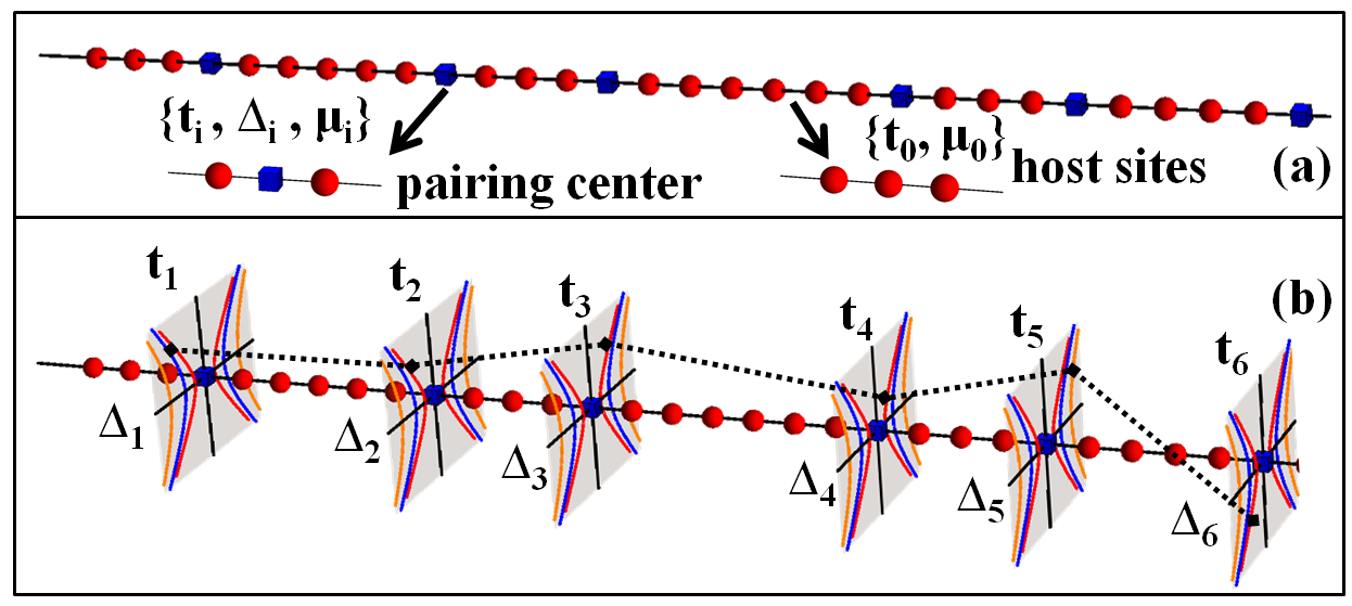
Figure 1: (a) Schematic representation of a large unit cell of length $L=30$ sites with $N=6$ impurities within the 1D chain with spatially inhomogeneous distributed PCs (blue squares) which separate host sites (red circles) and reduce the translational invariance. (b) A representative trajectory (dashed line) in the parameter space connecting different impurities in (a). Local variation along the hyperbolic contours in the shadow plane at the impurity site can lead to topologically equivalent non-trivial trajectories.

Symmetry features of the topological invariant.— The central result obtained in this paper is the general analytical expression for the topological invariant of an inhomogeneous quantum system. This outcome allows us to unveil the emergent symmetries in the parameter space and to predict the key physical regimes for the occurrence of Majorana end modes. By means of an inductive construction and a recursive relation in terms of the number of impurities within the unit cell, the coefficient $\cal A$ is

$${\cal A} \!= \cos\left(L\eta_{0}\right)\!+\sum_{i=1}^{N}y_{i}\sin\!\left(L\eta_{0}\right)$$

$$\!+ 2^{1}\sum_{i<j}y_{i}y_{j}\sin\!\left(d_{ij}\eta_{0}\right)\sin\!\left(d_{ji}\eta_{0}\right)$$

$$\!+ 2^{2}\!\sum_{i<j<k}\!\!y_{i}y_{j}y_{k}\sin\!\left(d_{ij}\eta_{0}\right)\sin\!\left(d_{jk}\eta_{0}\right)\sin\!\left(d_{ki}\eta_{0}\right)+\dots$$

$$\!+ 2^{N-1}y_{1}y_{2}\cdots y_{N}\!\sin\!\left(d_{12}\eta_{0}\right)\!\sin\!\left(d_{23}\eta_{0}\right)\cdots\sin\!\left(d_{N1}\eta_{0}\right),$$

where $d_{ij}$ are the ordered distances between impurities which cover the unit cell for each term of this expansion, i.e., $d_{ij}\equiv p_{j}-p_{i}$ for $j>i$ and $d_{ji}\equiv L-p_{j}+p_{i}$ for the second line, etcetera, see the Supplemental Material Sup . The above equation can be written in a compact form, ${\cal A}=\cos(L\eta_{0})+{\rm Tr}\{({\bf 1}-2{\bf M}_{1}{\bf Y})^{-1}{\bf M}_{2}^{T}{\bf Y}\}$, in terms of two triangular matrices of impurities’ distances ${\bf M}_{1}$ and ${\bf M}_{2}$, and a diagonal matrix ${\bf Y}$. These matrices have the following non-vanishing entries: $({\bf M}_{1})_{ij}=\sin(\eta_{0}d_{ij})$, $({\bf M}_{2})_{ij}=\sin(\eta_{0}(L-d_{ij}))$ for $j\geq i$ and ${\bf Y}_{ii}=y_{i}$. Here $\eta_{0}=\arccos(\mu_{0}/(2t_{0}))$ is the effective inverse Fermi length of the host, and $y_{i}$ are dimensionless variables related to the parameters at the impurity and in the host via

$$y_{i}=\frac{t_{0}(J_{i}^{-1}-J_{0}^{-1})}{\sqrt{4-\mu_{0}^{2}/t_{0}^{2}}},$$ (3)

with $J_{i}=(t_{i}^{2}-\Delta_{i}^{2})/\mu_{i}$ being a renormalized energy scale that includes effectively the particle- and hole-like transfer processes between the impurities and the host. Similarly, for the host one has $J_{0}=t_{0}^{2}/\mu_{0}$. Concerning ${\cal B}$ and ${\cal C}$, it is convenient to parametrize the set $\{t_{i},\Delta_{i},\mu_{i}\}$ at each host-impurity bond using hyperbolic coordinates as $t_{i}=r_{i}\cosh\phi_{i}$, $\Delta_{i}=r_{i}\sinh\phi_{i}$, and $\mu_{i}=r_{i}^{2}J_{i}^{-1}$, because they explicitly manifest their unique dependence on the hyperbolic angles as:

$${\cal B}=\cosh\left(2\sum_{i=1}^{N}\phi_{i}\right),\quad{\cal C}=\sinh\left(2\sum_{i=1}^{N}\phi_{i}\right).$$ (4)

Hence, the topological invariant has a highly symmetric structure in the parameter space. The coefficient ${\cal A}$ depends both on impurity-host and host bonds whereas the coefficients ${\cal B}$ and ${\cal C}$ contain only information about the impurity-host bonds through the sum of all hyperbolic angles. Note that the same properties hold in a general case of $\{t_{p},\Delta_{p},\mu_{p}\}$ taking arbitrary value on every bond/site, see the Supplemental Material Sup . Benefiting of the analytical expression of the winding number we can easily unveil hidden symmetries for the trajectories in the parameter space.

Firstly, a variation in the local angles $\{\phi_{i}\}$, akin to a relativistic Lorentz rotation, will not affect the amplitude of ${\cal B}$ as far as the sum of all angles stays unchanged. In this respect a given value of ${\cal B}$ corresponds to many equivalent trajectories in the $\{t_{i},\Delta_{i},\mu_{i}\}$ multidimensional space, see Fig. 1(b). In general it is always possible to turn the system topological by changing one hyperbolic angle to satisfy the condition $|{\cal A}|<|{\cal B}|$. This uncovers a novel non-local way to employ inhomogeneous perturbations for either driving a topological transition or for keeping unchanged the topological character of the ground state. Second symmetry aspect is related to the amplitude scaling of the impurity parameters. Indeed, a local scaling of $\mu_{i}$ and $r_{i}^{2}$ by the same factor will leave unchanged the amplitudes $\{y_{i}\}$. Moreover, either a cyclic translation of all the impurities in the unit cell or having a multiplied unit cell will not affect the coefficient ${\cal A}$.

Figure 2: Topological domains (blue regions) with: (a)-(d) small unit cells of the lengths $L=2,\dots,5$ with single impurity and $y_{i}\equiv y_{\rm imp}$, (e) doubled unit cell of $L=4$ and perturbed $y_{i}$, i.e., $y_{1}=y_{\rm imp}$ and $y_{2}=0.9\,y_{\rm imp}$ with impurities at regular position $p_{i}=4i$, and (f) ten-fold unit cell of $L=5$ and perturbed position of the last impurity by one bond, i.e., $p_{i}=5i$ for $i=1,\dots,9$ and $p_{10}=51$ with $y_{i}\equiv y_{\rm imp}$. Color map indicates values of $|{\cal A}|$ in the topological domains. Yellow regions are for topologically trivial configurations.

Finally, from the inspection of Eq. (LABEL:eq:master), we observe that there exists a special point in the parameter space where all $\{y_{i}\}$ vanish, i.e., at $J_{i}\equiv J_{0}$ which is a resonance condition between the host and impurities. Then, a special critical point emerges in the phase diagram where the interference between the impurities and the host makes ${\cal A}$ insensitive to the actual spatial distribution of impurities.

Periodic and disordered impurity pattern.— A topological domain can be obtained by imposing the condition $|{\cal A}|<1$. By construction $|{\cal B}|\geq 1$ so for any choice of hyperbolic angles $\{\phi_{i}\}$ such a region in the parameter space will be topologically non-trivial. For values $|{\cal A}|>1$ there can be regions with end Majorana mode, nevertheless their boundaries would be exponentially unstable to small changes in the parameters. In Figs. 2(a)-(d) we report the evolution of the topological domains for a single impurity unit cell in terms of the key physical parameters related to the impurity-host competition, i.e., $y_{i}\equiv y_{\rm imp}$ and $\mu_{0}/t_{0}$. The domains always extend around the line of impurity-host resonance at $y_{\rm imp}=0$ for which $|{\cal A}|\leq 1$. We observe that the topological domains evolve around the nodal lines of ${\cal A}$, and their number is $\lceil L/2\rceil$. Finally, for all the cases the topological regions never extend beyond $|\mu_{0}|=|2t_{0}|$ where the trigonometric functions in ${\cal A}$ become hyperbolic — this corresponds to the topological boundary of the pure Kitaev model Kitaev2001 .

The question of having slightly different $y_{i}$’s at two PCs is addressed in Fig. 2(e) when we double the unit cell of length $L=4$ [compare with Fig. 2(c)] and set $y_{1}=y_{\rm imp}$, $y_{2}=0.9\,y_{\rm imp}$. We see that the topological domains split into halves with narrow inclusions of the trivial phase and the number of nodal lines of ${\cal A}$ doubles. More splitting appear when we impose a small perturbation of impurity positions, see Fig. 2(f), by taking a ten-fold unit cell of $L=5$ [compare with Fig. 2(d)] and by moving one impurity (out of $N=10$) by one site.

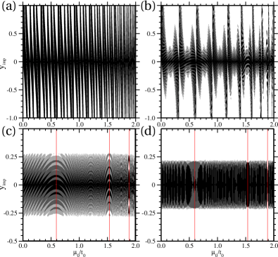
Figure 3: Topological domains (black) for equivalent PCs, $y_{i}\equiv y_{\rm imp}$, in: (a) a dimerized system with alternating distance between NN impurities $d_{1,2}\!=\!40$, $d_{2,1}\!=\!60$ and $L\!=\!100$, (b) a system with the unit cell of $L\!=\!1000$ and $N\!=\!20$ impurities with NN distances taking random and equiprobable value of $40$ or $60$, and (c) the same system with random distribution of impurities and $d_{ij}>1$. The random signs of $y_{i}$, i.e., $y_{i}\equiv\pm y_{\rm imp}$, are added to the case (c) in plot (d). Red lines indicate $\mu_{0}/t_{0}\simeq 0.6,1.54,1.9$, for which a zoomed view of the interference fringes is reported in the Supplemental Material Sup .

Topological domains persist for dilute impurities in large unit cells ($N\ll L$) as seen for a dimerized system with two distances between NN PCs, $d_{12}=40$ and $d_{21}=60$ ($L=100$) and $y_{i}\equiv y_{\rm imp}$, see Fig. 3(a). Next we randomize the NN distances so that for every bond $d_{i,i+1}=\{40,60\}$ with the same probability and implement the constraint that the total number of short/long bonds is the same. After averaging over $1000$ random configurations of unit cells with $L=1000$ and $N=20$ we obtain a complex interference pattern of many harmonics of $\eta_{0}$ which destroys some of the vertical legs of initial topological region of Fig. 3(a) and adds subtle parabolic modulation on top of it, see Fig. 3(b). Introducing complete randomness of the positions of PCs modifies the domains further, see Fig. 3(c). The long vertical legs are gone and the whole topological regions extend not beyond $|y_{\rm imp}|<0.25$. Interestingly the subtle parabolic features remain with some characteristic points on the horizontal axis (like $\mu_{0}/t_{0}=0.6,1.5,1.9$) around which the tips of many vertically shifted parabolas seems to accumulate. We note that adding even a significant random modulation of $y_{i}$ around $y_{\rm imp}$ does not change this result much as long as the signs of $y_{i}$ are fixed.

The parabolic features are suppressed and the domains gain a mirror symmetry around $y_{\rm imp}=0$ when signs of $\{y_{i}\}$ are random, see Fig. 3(d). Quite surprisingly, the characteristic $\mu_{0}/t_{0}$ points still host some distinct interference features. The overall width of the topological window is further reduced but only slightly. Note that lowering the concentration of PCs does not change much the subtle features of topological regions of Figs. 3(c) and 3(d) — only the width of the topological window is increased as the number of terms in ${\cal A}$ drops with $N$.

Conclusions.— We provide a novel perspective on the way to get Majorana end modes in 1D itinerant systems by means of an inhomogeneous distribution of PCs. The structure of the topological invariant uncovers the reasons why domains in the parameter space can be so robust to the local variations of impurity PCs. Such response to inhomogeneous perturbations is a generalization of the Kitaev model within the Altland-Zirnbauer classification and goes beyond the expectation from density disorder.

An interesting aspect of our analysis points to the possibility of having zero energy modes in the interior of the 1D diluted Kitaev chain. Such occurrence can be captured by searching for a parameter s configuration satisfying ${\cal C}=0$ and $|{\cal A}|\!<\!|{\cal B}|$. This condition implies that the determinant $\det[{\bf u}_{k}]$ vanishes at a given $k$. Hence, if the obtained zero energy states are not accidentally occurring at the boundary they must be in the interior of the system. Therefore, the combination of ${\cal C}=0$ and the topological regions for which $|{\cal A}|\!<\!|{\cal B}|$ makes a guide for the search of non-trivial states in the interior of the 1D diluted Kitaev chain. Another path to engineer inhomogeneous topological phases can be achieved by designing the system as a series of topologically inequivalent domains. For instance, by selecting the microscopic parameters for the impurity and the host such that the neighboring domains have different winding numbers (e.g. they are topologically inequivalent), Majorana modes would occur at the domain boundary in the interior of a quantum system.

Furthermore, for completeness, we observe that the modification of the kinetic term with the inclusion of long-range hopping is expected to lead to multiple Majorana end modes both in spinless DeGottardi2013a and spinfull $p$-wave SC chains Mercaldo2016 . We also point out that for the case of intrinsic diluted pairing centers, the model Hamiltonian in Eq. 1 would strictly apply only in the weak-coupling regime. Therefore, it is challenging to investigate to what extent the overall scenario will be modified by including finite NN interactions without any decoupling Kat15 .

Various realizations of the presented topological states may be possible. One way is to design a mesoscopic array of SC dots coupled to a metallic host in such a way that nearby the dot an effective spin-triplet pairing is induced, e.g. by employing spin-orbit and external magnetic field. Here, a local tuning of the superconducting amplitude can be achieved by external perturbations, while the hopping connectivity among the pairing centers might be tailored by the distance between the dots, or by suitably varying the conducting channels linking the dots. Another possible realization is in doped 1D spin-orbital quantum systems where coupling between host and dopants could be converted into effective pairing terms for the spin or the orbital channel. One could then atomically design doped quantum chains that map onto the Kitaev model Kitaev2001 with diluted PCs. Then, the present study may stimulate new directions of research on the generation and manipulation of Majorana states and their design for topological quantum computing Iva01 ; Nay08 .

We kindly acknowledge support by Narodowe Centrum Nauki (NCN) under Project No. 2012/04/A/ST3/00331. W. B. acknowledges financial support by the European Union’s Horizon 2020 research and innovation programme under the Marie Sklodowska-Curie Grant Agreement No. 655515. M. C. acknowledges support of the Future and Emerging Technologies (FET) programme under FET-Open Grant No. 618083 (CNTQC).

I Supplemental Material

In this Supplemental Material we present more details on the expansion of ${\cal A}$ in powers of $\{y_{i}\}$, link between the cases of uniform and alternating $\mu_{0}$ in the host and the generic form of coefficient ${\cal A}$ in case of arbitrary hopping amplitudes $t_{p}$, pairing amplitudes $\Delta_{p}$ and chemical potentials $\mu_{p}$ on every bond and site of the unit cell. Furthermore, we provide a zoomed view of the interference regions of the disordered phase diagram close to the resonant condition $y_{i}\equiv y_{\rm imp}$. Finally, a representative case for a fully disordered configuration is shown to demonstrate the occurrence and the character of the Majorana modes at the end sites of a chain of finite size.

I.1 A. Expansion of ${\cal A}$

Coefficients ${\cal B}$ and ${\cal C}$ (4) are rather easy to obtain so we first focus on ${\cal A}$. ${\cal A}$ is a combination of three determinants of tridiagonal matrices obtained from ${\bf u}_{k}$. These determinants can be further Laplace-expanded to separate the parameters of the impurities from the pure-host determinants. We set a uniform host, i.e., $\mu_{p}=\mu_{0}$ and $t_{p}=t_{0}$ for all host sites and bonds. The pure host determinant $D_{q}$ for $q$ host’s atoms between two impurities has a form of,

$$D_{q}=\det\begin{pmatrix}\mu_{0}&t_{0}&0&0\\ t_{0}&\ddots&\ddots&0\\ 0&\ddots&\mu_{0}&t_{0}\\ 0&0&t_{0}&\mu_{0}\end{pmatrix}.$$ (5)

Now it is important to notice that such a tridiagonal matrix can be diagonalized in terms of modes of a particle in a box with the resulting eigenvalues

$$\lambda_{q,n}=\mu_{0}-2t_{0}\cos\left(n\frac{\pi}{q+1}\right),$$ (6)

with $n=1,2,\dots,q$. The determinant is thus a product of these eigenvalues but it can be rephrased in terms of a trigonometric expression,

$$D_{q}=\frac{2\sin\left[(q+1)\eta_{0}\right]}{\sqrt{4-\mu_{0}^{2}/t_{0}^{2}}},$$ (7)

with

$$\eta_{0}=\arccos\frac{\mu_{0}}{2t_{0}}.$$ (8)

It is worth to notice that in fact $D_{q}\equiv U_{q}\left(\mu_{0}/2t_{0}\right)$, where $U_{n}(x)$ is a Chebyshev polynomial of the second kind of rang $n$. Note that $D_{q}$ is defined not only for $|\mu_{0}|<|2t_{0}|$ but also for any other $\mu_{0}$ by an analytical continuation of the arccos function. Similarly, the zeroth order term in $\{y_{i}\}$ appearing in the expansion of ${\cal A}$ is also a polynomial in $(\mu_{0}/2t_{0})$, i.e., the $L$-th Chebyshev polynomial of the first kind, $\cos(L\eta_{0})\equiv T_{L}\left(\mu_{0}/2t_{0}\right)$.

I.2 B. Alternating $\mu_{0}$ by a ’Wick rotation’

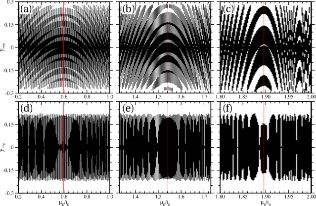
Figure 4: Zoomed view of the topological (black) domains of Fig. 3(c) (first row) and 3(d) (second row) of the main text close to specific values of $\mu_{0}/t_{0}$ (marked with red lines). The panels (a)-(c) refer to systems with a unit cell of $L\!=\!1000$ and $N\!=\!20$ randomly distributed impurities having the same $y_{i}\equiv y_{\rm imp}$ for $\mu_{0}/t_{0}\simeq 0.6,1.54,1.9$, respectively. The panels (d)-(f) refer to the same system size of (a)-(c) but with the inclusion of a random sign of $\{y_{i}\}$ around the same values of $\mu_{0}/t_{0}$.

Up to now we were working only in the uniform host limit where for all $\mu_{p}=\mu_{0}$ for all host’s sites. It is however surprisingly easy to switch to the case where the chemical potential of the host is alternating as $\mu_{p}=(-1)^{p}\mu_{0}$. Assume that $L$ is even, which is necessary, and for simplicity that there is only one impurity in the unit cell at site $p=L$. We get an anti-diagonal block ${\bf u}_{k}$ of ${\cal H}_{k}$ as,

$${\bf u}_{k}=-\begin{pmatrix}\mu_{1}&\tau_{L-1}^{-}&0&\cdots&e^{-ik}\tau_{L}^{+}\\ \tau_{L-1}^{+}&-\mu_{0}&\ddots&0&\vdots\\ 0&\ddots&\ddots&\tau_{2}^{-}&0\\ \vdots&0&\tau_{2}^{+}&-\mu_{0}&\tau_{1}^{-}\\ e^{ik}\tau_{L}^{-}&\cdots&0&\tau_{1}^{+}&\mu_{0}\end{pmatrix},$$ (9)

with $\tau_{p}^{\pm}\equiv t_{p}\pm\Delta_{p}$. Now we notice that the alternation in $\mu_{0}$ can be removed by multiplying ${\bf u}_{k}$ from left and from the right by a diagonal matrix ${\bf\sigma}$ having a diagonal of the form $\left\{1,i,1,i,\dots,1,i\right\}$. Denoting $\tilde{{\bf u}}_{k}={\bf\sigma}{\bf u}_{k}\sigma$ we get,

$$\tilde{{\bf u}}_{k}=-\begin{pmatrix}\mu_{1}&i\tau_{L-1}^{-}&0&\cdots&ie^{-ik}\tau_{L}^{+}\\ i\tau_{L-1}^{+}&\mu_{0}&\ddots&0&\vdots\\ 0&\ddots&\ddots&i\tau_{2}^{-}&0\\ \vdots&0&i\tau_{2}^{+}&\mu_{0}&i\tau_{1}^{-}\\ ie^{ik}\tau_{L}^{-}&\cdots&0&i\tau_{1}^{+}&\mu_{0}\end{pmatrix}.$$ (10)

This means that we are back in the uniform case because the determinant of ${\bf u}_{k}$ is proportional to the one of $\tilde{{\bf u}}_{k}$! More precisely, in the alternating case we are allowed to use the formulas for ${\cal A}$, ${\cal B}$ and ${\cal C}$ which were derived for the uniform case provided that we transform the parameters in the following way:

$$\mu_{0} \to \mu_{0}$$

$$t_{0} \to -it_{0}$$ (11)

for the host’s parameters and

$$\mu_{i} \to (-1)^{p_{i}}\mu_{i}$$

$$t_{i} \to -it_{i}$$

$$\Delta_{i} \to -i\Delta_{i}$$ (12)

for the impurities’ parameters, where $p_{i}$ is the position of the impurity $i$. Note that apart from the chemical potentials of the impurities this is indeed a Wick rotation of ${\cal A}$, ${\cal B}$ and ${\cal C}$ in terms of hopping and pairing amplitudes. It is straightforward to check that all these quantities remain real after such transformation.

Note that the main difference between the uniform and alternating case is as follows: For the uniform case the ${\cal A}$ coefficient in the limit of $|\mu_{0}|<|2t_{0}|$ is a sum of many sine and cosine functions that depend on angle $\eta_{0}$ so there are many interference terms expected and the profile of ${\cal A}$ is indeed very complicated. But in the opposite limit of $|\mu_{0}|>|2t_{0}|$ the trigonometric function become hyperbolic and consequently ${\cal A}$ will be roughly exponential in $\eta_{0}$ following the highest exponent $L\eta_{0}$. On the other hand, in the alternating regime, ${\cal A}$ will consist of hyperbolic functions for any values of $\mu_{0}$ so its profile will be much simpler. Since having a topological phase means having small ${\cal A}$, it will be much more difficult in the alternating regime than in the uniform one.

I.3 C. Coefficient ${\cal A}$ for arbitrary $\{t_{p},\Delta_{p},\mu_{p}\}$ on every bond and site

Setting the hyperbolic parametrization of the hopping and pairing amplitudes,

$$t_{p}=r_{p}\cosh\phi_{p},\hskip 19.91684pt\Delta_{p}=r_{p}\sinh\phi_{p},$$ (13)

for all sites and bonds in the unit cell one can show that the coefficient ${\cal A}$ can be expressed in terms of chemical potential and hyperbolic radii only as,

$${\cal A}=\frac{1}{2r_{1}r_{2}\cdots r_{L}}\begin{vmatrix}-\mu_{1}&r_{1}&0&0&r_{L}\\ r_{1}&-\mu_{2}&r_{2}&0&0\\ 0&r_{2}&-\mu_{3}&\ddots&0\\ 0&0&\ddots&\ddots&r_{L-1}\\ r_{L}&0&0&r_{L-1}&-\mu_{L}\end{vmatrix}+\left(-1\right){}^{L}.$$ (14)

Note that this expression has an explicit translation symmetry within the unit cell. The remaining ${\cal B}$ and ${\cal C}$ coefficients have an already the known form of Eqs. (4). Note that the hyperbolic parametrization not only covers the area of $t_{p}\geq 0$ and $|\Delta_{p}|<t_{p}$ but can be extended to the whole $t_{p}-\Delta_{p}$ plane (excluding the singular lines of $|\Delta_{p}|=|t_{p}|$) by analytical continuation of the inverse expressions, $r_{p}=\sqrt{t_{p}^{2}-\Delta_{p}^{2}}$ and $\phi_{p}={\rm arctanh}\left(\Delta_{p}/t_{p}\right)$, in the complex plane.

I.4 D. Additional features for a random distribution of impurities: zoomed view of the topological phase diagram and Majorana end modes

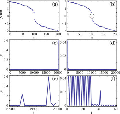
Figure 5: Energy spectra and edge states for a fully disordered 1D chain of size $L\!=\!20000$ and $N\!=\!200$ impurities assuming they are randomly distributed in space and the parameters correspond to $\{y_{i}\}=0$. (a)-(b) Spectra around zero energy for a closed system: (a) and the same spectrum for an open system and (b) exhibiting two zero energy states in the gap. Panel (c) indicates the occupation probability for the zero energy Majorana wave function versus the position $i$ at the right chain edge, with (e) being a zoomed view. (d) shows the occupation probability of the Majorana zero energy state projected at each position $i$ of the left chain edge. A zoomed view is given in (f).

In Fig. 4 we show the details of Figs. 3(c) and 3(d) as presented in the main text. A zoomed view of the topological domains around three selected values of $\mu_{0}/t_{0}$, i.e., $\mu_{0}/t_{0}\simeq 0.6,1.54,1.9$ is provided to identify better the observed self-similar features. In case of random positions of impurities and fixed $y_{i}\equiv y_{\rm imp}$ we see a parabolic pattern repeating itself which becomes increasingly narrow as we approach $\mu_{0}=2t_{0}$. This narrowing is related with the functional character of $\eta_{0}=\arccos(\mu_{0}/2t_{0})$, i.e., it has a singular derivative near $\mu_{0}=2t_{0}$. In case of random positions of the impurities and random sign of $\{y_{i}\}$ we do not observe such self-similarity but still distinct features are visible at $\mu_{0}/t_{0}\simeq 0.6,1.54,1.9$. We note that the horizontal resolution of the plots effectively decreases as we increase $\mu_{0}/t_{0}$ because we have an increasingly narrow window of $\mu_{0}/t_{0}$.

In Fig. 5 we report a representative case where the Majorana bound states appear at the end of the chain in a finite system when the condition for the topological invariant to be non-trivial is fulfilled. Indeed, we determine the energy spectra and the edge states for a system of $L\!=\!20000$ with $N\!=\!200$ randomly distributed impurities having all $\{y_{i}\}$ at the resonant condition $y_{i}=0$. This regime does not however imply that the impurities are identical, i.e., in terms of $\{t_{i},\Delta_{i},\mu_{i}\}$.

Using the hyperbolic parametrization, $t_{i}=r_{i}\cosh\phi_{i}$ and $\Delta_{i}=r_{i}\sinh\phi_{i}$, we can achieve the resonance condition $y_{i}=0$ by setting the host’s parameters at $t_{0}=\mu_{0}=1$ and the impurity’s chemical potential $\mu_{i}$ as $\mu_{i}=r_{i}^{2}$, see Eq. (3) in the main text. Thus, we are left with two free parameters, $r_{i}$ and $\phi_{i}$ at every impurity site. Then, one can randomly tune these amplitudes within the interval $[0,1]$. Here, we avoid negative angles for $\phi_{i}$ as they would lead to a vanishing $\sum_{i}\phi_{i}$ and, in turn, of the coefficient $\cal{C}$ (4), thus violating the necessary condition for having a fully gapped bulk spectrum.

In Figs. 5(a) and 5(b) we present the spectra around zero energy for a closed and open system, respectively. We note that for an open system there are two zero-energy states appearing in the energy gap. These are Majorana end modes that arise as a consequence of the bulk-boundary correspondence in a topologically non-trivial configuration. In Figs. 5(c) and 5(d) the spatial occupation probabilities in the two zero energy states is explicitly shown in order to confirm their degree of localization on the right/left edges of the 1D chain. Finally, in Figs. 5(e) and 5(f) we provide a zoomed view of the spatial distribution function just close to ends of the chain at the interface with the vacuum. As one can notice, the occupation probability for the two states is not symmetric due to the inversion symmetry breaking induced by the presence of a disordered pattern of pairing centers. Indeed, the occupation pattern reveals that Majorana wave function has an internal structure and involves only few sites for the left edge while it extends over more sites for the right edge boundary.

References

- (1) M. Z. Hasan and C. L. Kane, Rev. Mod. Phys. 82, 3045 (2010).
- (2) X.-L. Qi and S.-C. Zhang, Rev. Mod. Phys. 83, 1057 (2011).
- (3) C.-K. Chiu, J. C. Y. Teo, A. P. Schnyder, and S. Ryu, Rev. Mod. Phys. 88, 035005 (2016).
- (4) K. v. Klitzing, G. Dorda, and M. Pepper, Phys. Rev. Lett. 45, 494 (1980).
- (5) D. J. Thouless, M. Kohmoto, M. P. Nightingale, and M. den Nijs, Phys. Rev. Lett. 49, 405 (1982).
- (6) A. Y. Kitaev, AIP Conf. Proc. 1134, 22 (2009).
- (7) A. P. Schnyder, S. Ryu, A. Furusaki, and A. W. W. Ludwig, in Advances in Theoretical Physics: Landau Memorial Conference, edited by Lebedev and M. Feigel’man, AIP Conf. Proc. 1134 (AIP, Melville, NY, 2009), p.10.
- (8) X.-G. Wen, Phys. Rev. B 89, 035147 (2014).
- (9) L. Fu, C. L. Kane, and E. J. Mele, Phys. Rev. Lett. 98, 106803 (2007).
- (10) J. E. Moore and L. Balents, Phys. Rev. B 75, 121306(R) (2007).
- (11) R. Roy, Phys. Rev. B 79, 195322 (2009).
- (12) L. Fu, Phys. Rev. Lett. 106, 106802 (2011).
- (13) T. H. Hsieh, H. Lin, J. Liu, W. Duan, A. Bansi, and L. Fu, Nat. Commun. 3, 982 (2012).
- (14) K. Nomura, S. Ryu, M. Koshino, C. Mudry, and A. Furusaki, Phys. Rev. Lett. 100, 246806 (2008).
- (15) R. S. K. Mong, J. H. Bardarson, and J. E. Moore, Phys. Rev. Lett. 108, 076804 (2012).
- (16) L. Fu and C. L. Kane, Phys. Rev. Lett. 109, 246605 (2012).
- (17) K. Kobayashi, T. Ohtsuki, and K.-I. Imura, Phys. Rev. Lett. 110, 236803 (2013).
- (18) I. C. Fulga, B. van Heck, J. M. Edge, and A. R. Akhmerov, Phys. Rev. B 89, 155424 (2014).
- (19) P. Baireuther, J. M. Edge, I. C. Fulga, C. W. J. Beenakker, and J. Tworzydło, Phys. Rev. B 89, 035410 (2014).
- (20) B. Sbierski and P. W. Brouwer, Phys. Rev. B 89, 155311 (2014).
- (21) M. Diez, D. I. Pikulin, I. C. Fulga, and J. Tworzydło, New J. Phys. 17, 043014 (2015).
- (22) T. Morimoto, A. Furusaki, and C. Mudry, Phys. Rev. B 91, 235111 (2015).
- (23) J. Li, R.-L. Chu, J. K. Jain, and S.-Q. Shen, Phys. Rev. Lett. 102, 136806 (2009).
- (24) C. W. Groth, M. Wimmer, A. R. Akhmerov, J. Tworzydło, and C. W. J. Beenakker, Phys. Rev. Lett. 103, 196805 (2009).
- (25) I. Adagideli, M. Wimmer, and A. Teker, Phys. Rev. B 89, 144506 (2014).
- (26) W. Qin, D. Xiao, K. Chang, S.-Q. Shen, and Z. Zhang, arXiv:1509.01666 (2015).
- (27) L. Kimme and T. Hyart, Phys. Rev. B 93, 035134 (2016).
- (28) J. Röntynen and T. Ojanen, Phys. Rev. Lett. 114, 236803 (2015).
- (29) Q. Liu, C.-X. Liu, C. Xu, X.-L. Qi, and S.-C. Zhang, Phys. Rev. Lett. 102, 156603 (2009).
- (30) R. R. Biswas and A. V. Balatsky, Phys. Rev. B 81, 233405 (2010).
- (31) Y. L. Chen et al., Science 329, 659 (2010).
- (32) T. Schlenk et al., Phys. Rev. Lett. 110, 126804 (2013).
- (33) X.-L. Qi, T. L. Hughes, and S.-C. Zhang, Phys. Rev. B 78, 195424 (2008).
- (34) T.-P. Choy, J. M. Edge, A. R. Akhmerov, and C. W. J. Beenakker, Phys. Rev. B 84, 195442 (2011).
- (35) S. Nadj-Perge, I. K. Drozdov, B. A. Bernevig, and A. Yazdani, Phys. Rev. B 88, 020407(R) (2013).
- (36) S. Nakosai, Y. Tanaka, and N. Nagaosa, Phys. Rev. B 88, 180503(R) (2013).
- (37) J. Klinovaja, P. Stano, A. Yazdani, and D. Loss, Phys. Rev. Lett. 111, 186805 (2013).
- (38) B. Braunecker and P. Simon, Phys. Rev. Lett. 111, 147202 (2013).
- (39) M. M. Vazifeh and M. Franz, Phys. Rev. Lett. 111, 206802 (2013).
- (40) F. Pientka, L. I. Glazman, and F. von Oppen, Phys. Rev. B 88, 155420 (2013).
- (41) K. Pöyhönen, A. Westström, J. Röntynen, and T. Ojanen, Phys. Rev. B 89, 115109 (2014).
- (42) F. Pientka, L. I. Glazman, and F. von Oppen, Phys. Rev. B 89, 180505(R) (2014).
- (43) J. Li, T. Neupert, B. A. Bernevig, and A.Yazdani, Nat. Commun. 7, 10395 (2016).
- (44) A. Heimes, P. Kotetes, and G. Schon, Phys. Rev. B 90, 060507 (2014).
- (45) A. Heimes, D. Mendler, and P. Kotetes, New J. Phys. 17, 023051 (2015).
- (46) S. Nadj-Perge, I. K. Drozdov, J. Li, H. Chen, S. Jeon, J. Seo, A. H. MacDonald, B. A. Bernevig, and A. Yazdani, Science 346, 602 (2014).
- (47) R. Pawlak, M. Kisiel, J. Klinovaja, T. Meier, S. Kawai, T. Glatzel, D. Loss, and E. Meyer, Quantum Information 2, 16035 (2016).
- (48) A. Altland and M. R. Zirnbauer, Phys. Rev. B 55, 1142 (1997).
- (49) S. Tewari and J. D. Sau, Phys. Rev. Lett. 109, 150408 (2012).
- (50) S. Ryu, A. Schnyder, A. Furusaki, and A. Ludwig, New J. Phys. 12, 065010 (2010).
- (51) L. Fu and C. L. Kane, Phys. Rev. Lett. 100, 096407 (2008).
- (52) J. Alicea, Rep. Prog. Phys. 75, 076501 (2012).
- (53) C. W. J. Beenakker, Annu. Rev. Cond. Mat. Phys. 4, 113 (2013).
- (54) M. Leijnse and K. Flensberg, Semicond. Sci. Technol. 27, 124003 (2012).
- (55) P. Kotetes, New J. Phys. 15, 105027 (2013).
- (56) V. Mourik, K. Zuo, S. M. Frolov, S. R. Plissard, E. P. A. M. Bakkers, and L. P. Kouwenhoven, Science 336, 1003 (2012).
- (57) M. T. Deng, C. L. Yu, G. Y. Huang, M. Larsson, P. Caroff, and H. Q. Xu, Nano Lett. 12, 6414 (2012).
- (58) L. P. Rokhinson, Xinyu Liu, and J. K. Furdyna, Nat. Phys. 8, 795 (2012).
- (59) A. Das, Y. Ronen, Y. Most, Y. Oreg, M. Heiblum, and H. Shtrikman, Nat. Phys. 8, 887 (2012).
- (60) A. D. K. Finck, D. J. Van Harlingen, P. K. Mohseni, K. Jung, and X. Li, Phys. Rev. Lett. 110, 126406 (2013).
- (61) H. O. H. Churchill, V. Fatemi, K. Grove-Rasmussen, M. T. Deng, P. Caroff, H. Q. Xu, and C. M. Marcus, Phys. Rev. B 87, 241401(R) (2013).
- (62) M. Ruby, F. Pientka, Y. Peng, F. von Oppen, B. W. Heinrich, and K. J. Franke, Phys. Rev. Lett. 115, 197204 (2015).
- (63) S. M. Albrecht, A. P. Higginbotham, M. Madsen, F. Kuemmeth, T. S. Jespersen, J. Nygård, P. Krogstrup, and C. M. Marcus, Nature 531, 206 (2016).
- (64) O. Motrunich, K. Damle, and D. A. Huse, Phys. Rev. B 63, 224204 (2001).
- (65) W. DeGottardi, D. Sen, and S. Vishveshwara, New J. Phys. 13, 065028 (2011).
- (66) Y. Niu, S. B. Chung, C.-H. Hsu, I. Mandal, S. Raghu, and S. Chakravarty, Phys. Rev. B 85, 035110 (2012).
- (67) J. D. Sau, C. H. Lin, H.-Y. Hui, and S. Das Sarma, Phys. Rev. Lett. 108, 067001 (2012).
- (68) W. DeGottardi, D. Sen, and S. Vishveshwara, Phys. Rev. Lett. 110, 146404 (2013).
- (69) M. Tezuka and N. Kawakami, Phys. Rev. B 85, 140508(R) (2012).
- (70) L.-J. Lang and S. Chen, Phys. Rev. B 86, 205135 (2012).
- (71) P. W. Brouwer, M. Duckheim, A. Romito, and F. von Oppen, Phys. Rev. Lett. 107, 196804 (2011).
- (72) A. M. Lobos, R. M. Lutchyn, and S. Das Sarma, Phys. Rev. Lett. 109, 146403 (2012).
- (73) A. M. Cook, M. M. Vazifeh, and M. Franz, Phys. Rev. B 86, 155431 (2012).
- (74) F. L. Pedrocchi, S. Chesi, S. Gangadharaiah, and D. Loss, Phys. Rev. B 86, 205412 (2012).
- (75) J.-H. She, J. Fransson, A. R. Bishop, and A. V. Balatsky, Phys. Rev. Lett. 110, 026802 (2013).
- (76) J. Fransson, J. H. She, L. Pietronero, and A. V. Balatsky, Phys. Rev. B 87, 245404 (2013).
- (77) C. M. Varma, Phys. Rev. Lett. 61, 2713 (1988).
- (78) R. Micnas, J. Ranninger, and S. Robaszkiewicz, Rev. Mod. Phys. 62, 113 (1990).
- (79) Y. Bar-Yam, Phys. Rev. B 43, 359 (1991).
- (80) M. Dzero and J. Schmalian, Phys. Rev. Lett. 94, 157003 (2005).
- (81) M. Cuoco and J. Ranninger, Phys. Rev. B 70, 104509 (2004).
- (82) W. Brzezicki, A. M. Oleś, and M. Cuoco, Phys. Rev. X 5, 011037 (2015).
- (83) W. Brzezicki, M. Cuoco, and A. M. Oleś, J. Supercond. Novel Magn. 29, 563 (2016); 30, 129 (2017).
- (84) A. Kitaev, Phys. Usp. 44, 131 (2001).
- (85) Supplemental Material below, see for: (i) more details on the expansion of the and for (ii) a representative case of a fully disordered configuration.
- (86) W. DeGottardi, Ma. Thakurathi, S. Vishveshwara, and D. Sen, Phys. Rev. B 88, 165111 (2013).
- (87) M. T. Mercaldo, M. Cuoco, and P. Kotetes, Phys. Rev. B 94, 140503(R) (2016).
- (88) H. Katsura, D. Schuricht, and M. Takahashi, Phys. Rev. B 92, 115137 (2015).
- (89) D. A. Ivanov, Phys. Rev. Lett. 86, 268 (2001).
- (90) C. Nayak, S. H. Simon, A. Stern, M. Freedman, and S. Das Sarma, Rev. Mod. Phys. 80, 1083 (2008).