Deep Multi-view Models for Glitch Classification

Abstract

Non-cosmic, non-Gaussian disturbances known as “glitches”, show up in gravitational-wave data of the Advanced Laser Interferometer Gravitational-wave Observatory, or aLIGO. In this paper, we propose a deep multi-view convolutional neural network to classify glitches automatically. The primary purpose of classifying glitches is to understand their characteristics and origin, which facilitates their removal from the data or from the detector entirely. We visualize glitches as spectrograms and leverage the state-of-the-art image classification techniques in our model. The suggested classifier is a multi-view deep neural network that exploits four different views for classification. The experimental results demonstrate that the proposed model improves the overall accuracy of the classification compared to traditional single view algorithms.

Index Terms—  Multi-view learning, deep learning, image classification, neural network

1 INTRODUCTION

In many machine learning problems, samples are collected from more than one source. Also, various feature extraction methods can be used to provide more than one set of feature vectors per sample. Such extra sources or feature vectors are referred to as “views". Using multiple views can improve performance as they may provide complementary or redundant information [1].

Fusion of multiple sources of information has been used in many applications such as emotion recognition [2], recommendation systems [3], speech recognition [4, 5], and biometric verification [6]. Integrating multiple sources of data is a challenging task, and various approaches have been proposed in the literature [4][7]. More recently, deep learning techniques have shown promising performance for multi-modal fusion [8, 9, 10]. Moreover, deep learning methods have shown superb performance for many classification problems including image classification. In this paper, we propose deep multi-view models for a particular classification problem from the aLIGO project [11].

Advanced LIGO (Advanced Laser Interferometer Gravitational -wave Observatory, or aLIGO) has recently made the first direct observations of gravitational waves [12] [13], which are ripples in the fabric of spacetime caused by accelerating masses. Since aLIGO is sensitive to minuscule changes in distance, its experimental data is affected by a variety of non-cosmic disturbances. When such disturbances, called “glitches”, show up in the gravitational-wave data, they generally worsen the quality of the detection of candidate cosmic signals. The elimination and prevention of these glitches will improve the quality of the detection system and increase the chance of detecting gravitational waves. Therefore, it is necessary to develop methods for identifying and characterizing glitches, which will help to determine their origin and eliminate their cause. Since glitches can be visualized as time-frequency-energy images (spectrograms), image classification techniques can be used to identify and characterize them.

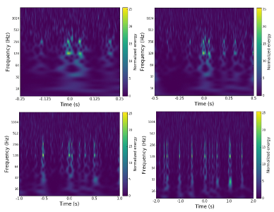
Fig. 1: An example of a Helix glitch with four views (Top from left to right: $0.5$ and $1.0$ seconds, bottom from left to right: $2.0$ and $4.0$ seconds).

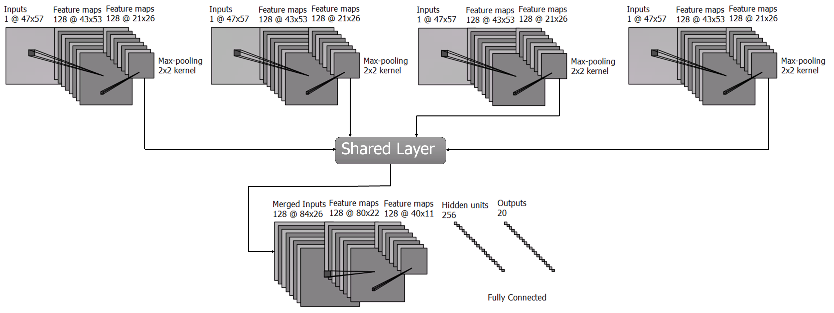
Fig. 2: Schematic representation of the “parallel view" model.

In this paper, we present the development of a multi-view deep neural network framework for glitch classification. Compared to standard methods that use just one set of images, we propose four-input models. We exploit four different time durations that are available for each glitch, namely each glitch plotted over time windows of $0.5$, $1$, $2$, and $4$ seconds. An example of such a glitch (from the “Helix” class) with four durations is shown in Fig. 1. We suggest two multi-view deep neural network models (a parallel view and a merged view) and we compare their performances to deep single view models. Experimental analysis shows that single view models trained with shorter glitches have a better performance for the classes that have shorter duration, while single view models trained with longer-duration glitches work better for long-duration classes. Our experimental results show that the developed multi-view framework improves the glitch classification accuracy by capturing the required information from glitches of various morphological characteristics.

The rest of this paper is organized as follows. In the next section, we present our model. Experiments and results are discussed in Section 3. We conclude this paper in Section 4.

2 THE PROPOSED MODEL

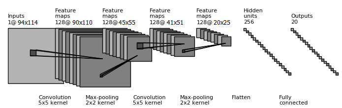
Fig. 3: Architecture of the “merged view” model.

Table 1: Best Models Specifications

Single view models Parallel view model Merged view model Input $1\times 47\times 57$ Input four $1\times 47\times 57$ Input $1\times 94\times 114$ $5\times 5$ Conv- $128$, $2\times 2$ Maxpooling, ReLU Four $5\times 5$ Conv- $128$, $2\times 2$ Maxpooling, ReLU $5\times 5$ Conv- $128$, $2\times 2$ Maxpooling, ReLU $5\times 5$ Conv- $128$, $2\times 2$ Maxpooling, ReLU $5\times 5$ Conv- $128$, $2\times 2$ Maxpooling, ReLU $5\times 5$ Conv- $128$, $2\times 2$ Maxpooling, ReLU Fully Connected-$256$ Fully Connected-$256$ Fully Connected-$256$ Sofmax-$20$ Sofmax-$20$ Sofmax-$20$

The main motivation for this study is to exploit multiple views for glitch classification instead of depending on just a single view. We investigate this by combining views’ information at two points as we go through the deep network layers. We thus propose one model in which fusion take place at an early step (referred to as “merged view”) and one in which information is integrated at the middle level (referred to as “parallel view”). In the following sections we explain these two architectures in detail.

2.1 Parallel view model

The idea behind the parallel view model is to project each view into a feature space which is based more on the statistical properties of the samples than their view-specific properties. This projection makes the views interact with each other and be presented in a common feature space more efficiently. We illustrate the construction of the parallel view model using the four durations as views in Fig. 2. At the very first layer, each view passes through a convolutional layer, followed by max-pooling and ReLU activation. Then, we introduce a shared layer (merger layer) to map all views into a common feature space. Another set of convolutional, max-pooling, and activation layers is used after the merger layer to model the obtained common features from the previous layers. In the end, a fully connected layer and a softmax layer are employed (see Fig. 2).

2.2 Merged view model

In this model, we introduce the network layers on top of the merged views. We merge the views by forming a $2m\times 2k$ matrix by placing next to each other four $m\times k$ images. After merging the views, a set of convolutional layer followed by max-pooling and activation layer is used, and then a fully connected layer and a softmax layer are exploited (see Fig. 3). This approach clearly models jointly the distribution of the different views in their original feature space. This seems a reasonable approach since the correlations among the views in our problem are not highly non-linear compared to other tasks where the views are very different, such as image and text [8], or audio and video [9]. Therefore it is possible for the model to learn such correlations even in the original space of data.

2.3 Training

The models presented above optimize a loss function defined on the training data. For training the model, we can use either the mean squared error or the average cross-entropy error as the loss function. Due to the advantages of the average cross-entropy error over the mean squared error, e.g., the derivation of a “better” gradient for back propagation, for multi-class classification problems [14], in our model we use a cross-entropy based loss function defined as follows:

$$E=-\sum_{n=1}^{N}\sum_{i=1}^{C}y_{i}^{n}\log o_{i}^{n}$$ (1)

where $o_{i}^{n}$ is the model’s output for class $i$ when the $n^{\textrm{{th}}}$ training sample is given to the network, $y_{i}^{n}$ is one if the $n^{\textrm{{th}}}$ sample is from class $i$, otherwise it is zero, and $N$ and $C$ are the total numbers of the training samples and classes, respectively. There exits many optimization techniques [15, 16, 17, 18] that we can use to optimize the objective function. We use the Adadelta [15] optimizer. It monotonically decreases the learning rate and shows good performance in our experiments.

3 EXPERIMENTS AND RESULTS

3.1 Dataset

The dataset consists of glitch samples from $20$ classes. The glitches are represented as a spectrogram, a time-frequency representation where the x-axis represents the duration of the glitch and the y-axis shows the frequency content of the glitch. The colors indicate the “loudness” of the glitch in the aLIGO detector. The classes arise from different environmental and instrumental mechanisms, and are based on the shape and intensity of the glitch in time-frequency space. The primary sample duration is $0.5$ second. However, in this study we use three other durations, i.e., $1.0$, $2.0$ and $4$ seconds, per glitch to train our multi-view models. An example of the dataset with four durations is shown in the Fig. 1. In total, there are $7730$ glitches in our dataset. We use $75\%$, $12.5\%$, and, $12.5\%$ of samples as training, validation, and test sets, respectively.

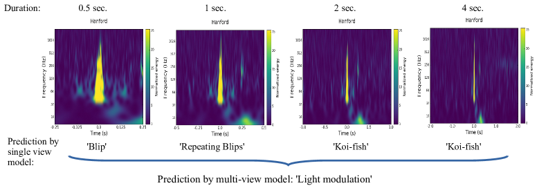
Fig. 4: An example of a glitch that was misclassified by all four single view models, but correctly classified with both of the multi-view models. The single view model, which is trained with $0.5$ second duration images, classifies it as “Blip” class. The predicted class is “Repeating Blips”, “Koi fish”, and “Koi fish” for the single view models trained with $1$, $2$, and $4$ second duration glitches, respectively. Multi-view models predict the sample correctly as belongs to the “Light Modulation” class.

3.2 Experiment

Baseline
A straightforward approach is to use just one glitch duration, as is done in a traditional single view approach. We use this as a baseline to compare the performance of our multi-view deep models. For single view models, we use CNNs with the structure shown in Table 1 (left column). The architecture of CNNs is optimized for the best classification accuracy. We use two convolutional layers with $128$ kernels of size $5\times 5$, max-pooling of $2\times 2$, and the ReLU activation function. Batch size is set to $30$, and the number of iterations is $130$. In Table 2, the classification accuracies of single view CNNs are presented.

Table 2: Classification accuracy of single view CNNs. The best model shows $95.34\%$ obtained from the model trained with $1$ second glitches. It seems that Classifier $2$ can capture the required information of both long and short duration classes better compared to the Classifier $1$ (trained with short durations) and Classifier $3$ and $4$ (trained with long durations).

Classifier	Duration	Accuracy ($\%$)
Classifier $1$	$0.5$ second	92.85
Classifier $2$	$1$ second	95.34
Classifier $3$	$2$ seconds	94.09
Classifier $4$	$4$ seconds	93.68

Deep multi-view models
In the parallel view model, first, we use four separate convolutional layers (see Fig. 2). Each has $128$ kernels with size $5\times 5$, and $2\times 2$ max-pooling and ReLu activation. Then, we merge the output of these four convolutional layers into the merger layer and use another convolutional layer with the same structure, and finally a fully connected layer with $256$ nodes and a softmax layer with $20$ nodes (equal to the number of classes). All these details are shown in the middle column of Table 1. The parameters of this architecture were obtained based on extensive experimentation and guidance from literature.

In the merged view model, we use the structure shown in Fig. 3. Two convolutional layers with $128$ kernel of size $5\times 5$, max-pooling of $2\times 2$, and ReLU activation function are used. One fully connected layer with $256$ nodes and softmax with $20$ outputs are added to the model. All details are shown in the right column of Table 1.

For both structures, the number of iterations is set to $130$ and the batch size is $30$. We use Keras [19] with Theano [20] back-end for all implementations. In Table 3, the best performances of parallel and merged view models are compared with the best single view model performance. See Table 1 for full models specifications.

Table 3: Classification accuracy of single and multi-view CNNs.

Classifier	Accuracy ($\%$)
The best single view model	95.34
parallel view model	95.75
merged view model	96.89

Table 4: Classification accuracy of single view model trained with one second duration (classifier $1$) and four second duration (classifier $4$) for each class. The first column shows whether the class is a short (Sh) or long (L) duration.

Duration Class Classifier 1 Acc. ($\%$) Classifier 4 Acc. ($\%$) Sh Air Compressor 100.00 80.00 Sh Blip 98.09 97.61 Sh Helix 96.66 96.66 Sh Power Line 100.00 100.00 Sh Repeating Blips 80.00 76.00 Sh Tomte 100.00 100.00 L Extremely Loud 96.77 98.38 L Light Modulation 83.14 86.51 L Low Frequency Lines 89.79 89.79 L Scattered Light 98.36 98.36 L Wandering Line 57.14 71.42

3.3 Analysis

As the results in Table 3 show, the performance of multi-view deep models is better than single view models. An example of a misclassified sample by all single view models that was classified correctly by the multi-view models is shown in Fig. 4. Such examples show that in many cases, single view models do not have the needed sight and horizon for recognizing glitches correctly. Glitch classes are divided into short and long duration based on the glitch duration. In Table 4, we show the category of each class plus the accuracy of two of the single view models; the 0.5-second model (Classifier $1$) and 4-second model (Classifier $4$). As can be seen in this table Classifier $1$ performs at least as good as Classifier $4$ for short duration glitches, while the opposite is true for long duration glitches, as expected for some classes (e.g., “Air Compressor” and “Tomte”) the performance is perfect with both classifiers. Clearly the multi-view models which use all durations can capture the needed information to classify all types of glitches (according to their duration) more accurately.

4 CONCLUSIONS

In this paper, we proposed multi-view deep neural network models for the glitch classification problem in aLIGO data. Two multi-view models, merged view and parallel view, are presented. The parallel view model projects samples into a common feature space where the views can interact efficiently. In the merged view model, the deep model is introduced on the concatenated durations. The experimental results show that multi-view models provide higher classification accuracy compared to the single view models, since they can accommodate efficiently the various classes independently of the glitch durations.

5 ACKNOWLEDGMENT

This work was supported in part by an NSF INSPIRE grant (award number IIS-1547880). The authors would like to thank Joshua Smith from California State - Fullerton University for being the chief point of contact between this study and the LIGO detector characterization working group and for being a resource on LIGO glitches and current methods of data analysis.

References

- [1] C. Xu, D. Tao, and C. Xu, “A survey on multi-view learning,” arXiv preprint arXiv:1304.5634, 2013.
- [2] X. Huang, J. Kortelainen, G. Zhao, X. Li, A. Moilanen, T. Seppänen, and M. Pietikäinen, “Multi-modal emotion analysis from facial expressions and electroencephalogram,” Computer Vision and Image Understanding, vol. 147, pp. 114–124, 2016.
- [3] L. Zheng, V. Noroozi, and Ph. S. Yu, “Joint deep modeling of users and items using reviews for recommendation,” in ACM International Conference on Web Search and Data Mining (WSDM), 2017.
- [4] A. K. Katsaggelos, S. Bahaadini, and R. Molina, “Audiovisual fusion: Challenges and new approaches,” Proceedings of the IEEE, vol. 103, no. 9, pp. 1635–1653, Sept 2015.
- [5] S. Bahaadini, A. Asaei, D. Imseng, and H. Bourlard, “Posterior-based sparse representation for automatic speech recognition,” Proceeding of Interspeech, 2014.
- [6] P. S. Aleksic and A. K. Katsaggelos, “An audio-visual person identification and verification system using faps as visual features,” in ACM Workshop on Multimodal User Authentication. Citeseer, 2003, pp. 80–84.
- [7] N. Rohani, P. Ruiz, E. Besler, R. Molina, and A. K. Katsaggelos, “Variational gaussian process for sensor fusion,” in Signal Processing Conference (EUSIPCO), 2015 23rd European, Aug 2015, pp. 170–174.
- [8] N. Srivastava and R. R. Salakhutdinov, “Multimodal learning with deep boltzmann machines,” in Advances in neural information processing systems, 2012, pp. 2222–2230.
- [9] J. Ngiam, A. Khosla, M. Kim, J. Nam, H. Lee, and A. Ng, “Multimodal deep learning,” in Proceedings of the 28th international conference on machine learning (ICML-11), 2011, pp. 689–696.
- [10] H. Suk, S. Lee, and D. Shen, “Hierarchical feature representation and multimodal fusion with deep learning for ad/mci diagnosis,” NeuroImage, vol. 101, pp. 569–582, 2014.
- [11] M. Zevin, S. Coughlin, S. Bahaadini, E. Besler, N. Rohani, S. Allen, M. Cabero, K. Crowston, A. Katsaggelos, Sh. Larson, et al., “Gravity spy: Integrating advanced ligo detector characterization, machine learning, and citizen science,” arXiv preprint arXiv:1611.04596, 2016.
- [12] B. P. Abbott, R. Abbott, T. D. Abbott, M. R. Abernathy, F. Acernese, K. Ackley, C. Adams, T. Adams, P. Addesso, R. X. Adhikari, and et al., “Observation of Gravitational Waves from a Binary Black Hole Merger,” Physical Review Letters, vol. 116, no. 6, pp. 061102, Feb. 2016.
- [13] B. P. Abbott, R. Abbott, T. D. Abbott, M. R. Abernathy, F. Acernese, K. Ackley, C. Adams, T. Adams, P. Addesso, R. X. Adhikari, and et al., “GW151226: Observation of Gravitational Waves from a 22-Solar-Mass Binary Black Hole Coalescence,” Physical Review Letters, vol. 116, no. 24, pp. 241103, June 2016.
- [14] P. Golik, P. Doetsch, and H. Ney, “Cross-entropy vs. squared error training: a theoretical and experimental comparison.,” in INTERSPEECH, 2013, pp. 1756–1760.
- [15] M. D. Zeiler, “Adadelta: an adaptive learning rate method,” arXiv preprint arXiv:1212.5701, 2012.
- [16] Diederik P. Kingma and Jimmy Ba, “Adam: A method for stochastic optimization,” CoRR, vol. abs/1412.6980, 2014.
- [17] V. Noroozi, A. Hashemi, and M.R Meybodi, “Alpinist cellularde: a cellular based optimization algorithm for dynamic environments,” in Proceedings of the 14th annual conference companion on Genetic and evolutionary computation. ACM, 2012, pp. 1519–1520.
- [18] A. Sharifi, V. Noroozi, M. Bashiri, A. Hashemi, and M.R. Meybodi, “Two phased cellular pso: A new collaborative cellular algorithm for optimization in dynamic environments,” in 2012 IEEE Congress on Evolutionary Computation. IEEE, 2012, pp. 1–8.
- [19] F. Chollet, “Keras,” https://github.com/fchollet/keras, 2015.
- [20] J. Bergstra, O. Breuleux, Fr. Bastien, P. Lamblin, . Pascanu, G. Desjardins, J. Turian, D. Warde-Farley, and Y. Bengio, “Theano: a CPU and GPU math expression compiler,” in Proceedings of the Python for Scientific Computing Conference (SciPy), June 2010, Oral Presentation.