Squeezing and EPR correlation in the Mirrorless Optical Parametric Oscillator

Abstract

This work analyses the quantum properties of counter-propagating twin beams generated by a Mirrorless Optical Parametric Oscillator in the continuous variable regime. Despite the lack of the filtering effect of a cavity, we show that in the vicinity of its threshold it may generate high levels of narrowband squeezing and Einstein-Podolsky-Rosen (EPR) correlation, completely comparable to what can be obtained in standard optical parametric oscillators.

Backward parametric down-conversion (PDC), where one of the twin beams back-propagates with respect to the pump laser source (Fig.1), is gaining an increasing attention in the quantum optics community. In the spontaneous regime it has a natural potentiality to generate high-purity and narrowband heralded single photons Christ et al. (2009); Gatti et al. (2015); Brambilla et al. (2016), a highly desirable and non trivial goal, which in the standard co-propagating geometry can be realized only at specific tuning points.

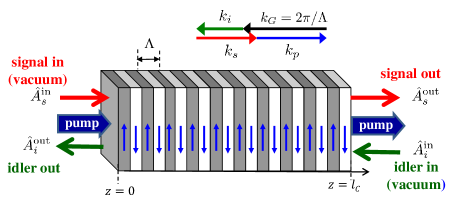
Figure 1: (Color online)Scheme of backward PDC, taking place in a $\chi^{(2)}$ crystal periodically poled with a submicrometer period $\Lambda\approx\lambda_{p}/n_{p}$. Quasi-phase matching [Eq.(1)] requires then that the idler field is generated in the backward direction with respect to the signal and pump.

A second appealing feature is the presence of a threshold pump intensity, beyond which the system makes a transition to coherent oscillations, i.e. it behaves as a Mirrorless Optical parametric Oscillator (MOPO)Canalias and Pasiskevicius (2008). Responsible of this critical behaviour is the feedback mechanism established by back-propagation and stimulated down-conversion. Ref. Corti et al. (2016) analysed the critical behavior of twin beams below threshold, enlightening the role of the quantum correlation of photon pairs in creating the feedback necessary to the onset of a classical coherence above threshold.

In this work we turn our attention to the quantum properties of the source in the continuous-variable regime, so far unexplored, namely its potentiality to generate EPR-correlated beams in the vicinity of the threshold. EPR correlation Einstein et al. (1935); Reid (1989); Ou et al. (1992), i.e. nonclassical correlations in a pair of non-commuting field quadratures, and their associated squeezing, are features of the two -mode squeezed state produced by any down-conversion process (see e.g.Gerry and Knight (2005)). However, squeezed light generated in the standard single-pass configuration is in general multimode, which is often undesirable for applications Lemieux et al. (2016) Moreover high levels of squeezing are hard to be generated and detected (see e.g. La Porta and Slusher (1991), but also Eto et al. (2008); Kaiser et al. (2016) for recent achievements in this sense). The typical solution is to recycle the parametric light in an optical resonator, which at the same time enforces the nonlinearity and produces a sharp modal filtering, i.e. to build an optical parametric oscillator (OPO). Remarkably, this work will show that counterpropagating twin-beams, despite the lack of the filtering effect of the cavity, exhibit high levels of narrowband EPR correlation, completely comparable to what can be obtained in standard subthreshold OPOs. The role of the cavity is in the MOPO played by the distributed feedback mechanismCorti et al. (2016), which creates a threshold where, similarly to the OPO, the quantum noise in principle diverges in some observables, allowing then noise suppression in their conjugate observables. Once technical challenges involved in its realization are overcome, this source may then represent a robust and compact alternative to the OPO.

The backward geometry requires a sub-micrometer poling of the $\chi^{(2)}$ materials, which explains why after the first theoretical prediction Harris (1966), this source had to wait forty years before being realized Canalias and Pasiskevicius (2008). We consider the scheme in Fig.1, in which the laser pump at frequency $\omega_{p}$ and the signal at frequency $\omega_{s}$ co-propagate along the $+z$ axis in the nonlinear medium, while the idler at frequency $\omega_{i}=\omega_{p}-\omega_{s}$ back-propagates in the $-z$ direction. Quasi-phase matching (i.e. the generalized momentum conservation) is realized when their corresponding wave numbers $k_{j}=\omega_{j}\,n_{j}(\omega_{j})/{c}$ satisfy

$$k_{s}-k_{i}=k_{p}-m\frac{2\pi}{\Lambda}\qquad m=1,3\ldots$$ (1)

where $\Lambda$ is the poling period, and $n_{j}$ the refraction indexes. First order interactions then require $\Lambda\simeq\lambda_{p}/n_{p}$.

Our quantum model for this configuration was described in Refs.Corti et al. (2016); Gatti et al. (2015) (see also Suhara and Ohno (2010)). As in the former literature, we restrict to a purely temporal description, assuming either waveguiding or a small collection angle. Below the MOPO threshold the depletion of the pump laser is negligible, and it can be described as a classical field of constant amplitude along the sample. Assuming in addition that the pump is CW, it is simply described by its complex amplitude $\alpha_{p}=|\alpha_{p}|e^{i\phi_{p}}$. The strength of the parametric interaction is then characterized by the dimensionless gain

$$g=\sqrt{2\pi}\chi|\alpha_{p}|l_{c}$$ (2)

where $\chi$ is proportional to the $\chi^{(2)}$ susceptibility of the medium and $l_{c}$ is the crystal length. In terms of this parameter the MOPO threshold occurs Ding and Khurgin (1996) at

$$g=g_{\mathrm{thr}}=\frac{\pi}{2}$$ (3)

The signal and idler waves are instead described by quantum field operators $\hat{A}_{s}(\Omega,z)$ and $\hat{A}_{i}(\Omega,z)$, for two wavepackets centered around the respective reference frequencies $\omega_{s}$ and $\omega_{i}$ satisfying quasi-phasematching (1) (capital $\Omega$ is the offset from the $\omega_{j}$). As detailed in Corti et al. (2016), the model is formulated in terms of linear propagation equations coupling only frequency conjugate modes $\omega_{s}+\Omega$, $\omega_{i}-\Omega$ of the twin beams, whose solution gives a transformation linking the output operators $\hat{A}_{s}^{\text{out}}=\hat{A}_{s}(z=l_{c})$, $\hat{A}_{i}^{\text{out}}=\hat{A}_{i}(z=0)$ to the input ones (Fig.1), assumed in the vacuum state. Notice that in this geometry the boundary conditions are not the standard ones, because the signal and idler fields exit from the opposite end faces of the slab. The input-ouput relations are then the Bogoliubov transformation, characteristic of processes where particles are generated in pairs:

$$\hat{A}_{s}^{\text{out}}(\Omega) =U_{s}(\Omega)\hat{A}_{s}^{\text{in}}(\Omega)+V_{s}(\Omega)\hat{A}_{i}^{\text{in}\dagger}(-\Omega)$$ (4a)

$$\hat{A}_{i}^{\text{out}}(-\Omega) =U_{i}(-\Omega)\hat{A}_{i}^{\text{in}}(-\Omega)+V_{i}(-\Omega)\hat{A}_{s}^{\text{in}\dagger}(\Omega).$$ (4b)

The coefficients $U_{j}(\Omega)$ and $V_{j}(\Omega)$ are the trigonometric functions Corti et al. (2016):

$$U_{s}(\Omega) =e^{ik_{s}l_{c}}e^{i\beta(\Omega)}\phi(\Omega)$$ (5a)

$$V_{s}(\Omega) =e^{i(k_{s}-k_{i})l_{c}}ge^{i\phi_{p}}\frac{\sin\gamma(\Omega)}{\gamma(\Omega)}\phi(\Omega)$$ (5b)

$$U_{i}(-\Omega) =e^{ik_{i}l_{c}}e^{i\beta(\Omega)}\phi^{*}(\Omega)$$ (5c)

$$V_{i}(-\Omega) =ge^{i\phi_{p}}\frac{\sin\gamma(\Omega)}{\gamma(\Omega)}\phi^{*}(\Omega)\qquad\text{with}$$ (5d)

$$\phi(\Omega) =\frac{1}{\cos\gamma(\Omega)-i\frac{\bar{\mathcal{D}}(\Omega)l_{c}}{2\gamma(\Omega)}\sin\gamma(\Omega)}$$

$$\gamma(\Omega) =\sqrt{g^{2}+\frac{{\mathcal{D}}^{2}(\Omega)l_{c}^{2}}{4}},$$ (5e)

In these expressions:

$${\mathcal{D}}(\Omega) =k_{s}(\Omega)-k_{i}(-\Omega)-k_{p}+k_{G}$$ (6)

is the phase mismatch for two frequency conjugate signal-idler components, $k_{j}(\Omega)$ being the wavenumber of $j-$th wave at frequency $\omega_{j}+\Omega$ ($j=s,i$). The phase

$$\beta(\Omega)=[k_{s}(\Omega)+k_{i}(-\Omega)-(k_{s}+k_{i})]\frac{l_{c}}{2}$$ (7)

is a global propagation phase. Notice that the coefficients $U_{j}(\Omega)$ and $V_{j}(\Omega)$ diverge when approaching the MOPO threshold $g=\pi/2$, and, as can be easily checked, they satisfy the unitarity conditions: $|U_{j}(\Omega)|^{2}-|V_{j}(\Omega)|^{2}=1$, and $U_{s}(\Omega)V_{i}(-\Omega)=U_{i}(-\Omega)V_{s}(\Omega)$

Unlike the co-propagating case, this configuration is characterized by narrow spectral bandwidths Canalias and Pasiskevicius (2008); Gatti et al. (2015); Corti et al. (2016). Therefore, it is legitimate to retain only the first order of the Taylor expansions of the wavenumbers $k_{j}(\Omega)$, so that

$$\frac{{\mathcal{D}}(\Omega)l_{c}}{2} \simeq\frac{l_{c}}{2}(k_{s}^{\prime}+k_{i}^{\prime})\Omega:=\frac{\Omega}{{\Omega_{\mathrm{gvs}}}}$$ (8)

$$\beta(\Omega) \simeq(k^{\prime}_{s}-k^{\prime}_{i})\frac{l_{c}}{2}\Omega=\frac{\Omega}{{\Omega_{\mathrm{gvm}}}},$$ (9)

where $k^{\prime}_{j}=\frac{dk_{j}}{d\Omega}|_{\Omega=0}$ , and

$$\Omega_{\mathrm{gvs}}^{-1}\equiv{\tau_{\mathrm{gvs}}}=\frac{1}{2}\left[\frac{l_{c}}{v_{gs}}+\frac{l_{c}}{v_{gi}}\right].$$ (10)

is a long time scale characteristic of counterpropagating interactions, on the order of the transit time of light along the slab, involving the sum of the inverse group velocities $v_{gj}=1/k^{\prime}_{j}$ Corti et al. (2016); Gatti et al. (2015). In the spontaneous regime, it defines the correlation time of twin photons, while its inverse ${\Omega_{\mathrm{gvs}}}$ gives the narrow width of their spectrum, which becomes even narrower in the stimulated regime and ideally shrinks to zero on approaching threshold Corti et al. (2016). Conversely

$$\Omega_{\mathrm{gvm}}^{-1}\equiv{\tau_{\mathrm{gvm}}}=\frac{l_{c}}{2v_{gs}}-\frac{l_{c}}{2v_{gi}}$$ (11)

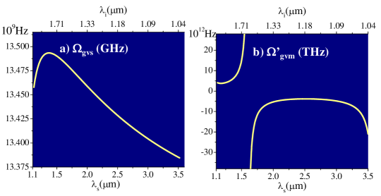
Figure 5: (Color online) Comparison between the two spectral scales of the MOPO for PPLN pumped at 800 nm, $l_{c}=1cm$. a) ${\Omega_{\mathrm{gvs}}}=\frac{2}{l_{c}}({k^{\prime}_{s}+k^{\prime}_{i}})^{-1}\simeq 10$Ghz is the narrow MOPO bandwidth; b) ${\Omega_{\mathrm{gvm}}}=\frac{2}{l_{c}}({k^{\prime}_{s}-k^{\prime}_{i}})^{-1}$ in the range 5Thz or more is the broader GVM bandwidth. For each $\lambda_{s},\lambda_{i}$ the poling period is chosen to realize phase-matching according to Eq.(1).

is a short time scale related to the group velocity mismatch (GVM), and produces a small temporal offset between the signal and idler wave-packets. Clearly, $|{\Omega_{\mathrm{gvm}}}|\gg{\Omega_{\mathrm{gvs}}}$ for any tuning conditions (see Fig.5 for a comparison in the case of LiNbO₃). Within these linear approximations the coefficients $U_{j}(\Omega)$ and $V_{j}(\Omega)$ basically depend on the frequency only through the ratio $\frac{\Omega^{2}}{\Omega^{2}_{\mathrm{g}vs}}$, because $\gamma(\Omega)\simeq\sqrt{g^{2}+\frac{\Omega^{2}}{\Omega^{2}_{\mathrm{g}vs}}},$ while the phase $\beta(\Omega)$ in (9) varies on the slow scale $|{\Omega_{\mathrm{gvm}}}|\gg{\Omega_{\mathrm{gvs}}}$ and remains close to zero in the spectral region where $U_{j}(\Omega)$ and $V_{j}(\Omega)$ take non trivial values.

Several properties of the state of the MOPO below threshold depend solely on the Bogoliubov form (4) of the transformation, so that they are common to any linear process of photon-pair generation. In particular, if one introduces the sum and difference between frequency conjugate components of the twin beams: $\hat{C}_{\pm}(\Omega)=\frac{1}{\sqrt{2}}[\hat{A}_{s}^{\mathrm{o}ut}(\Omega)\pm A_{i}^{\mathrm{o}ut}(-\Omega)],$ then the transformation (4) decouples into two independent squeeze transformationsGatti et al. (2017). The $\pm$ modes are thus individually squeezed, and their squeezing ellipses turn out oriented along orthogonal directions. As well known, this implies the simultaneous presence of correlation and anticorrelation in two orthogonal quadrature operators of the twin beams Reid (1989); Ou et al. (1992).

In order to characterize the amount of squeezing and EPR correlation generated in this specific configuration, let us consider the quadrature operators for the individual signal and idler fields in the time domain

$$\hat{X}_{j}(t) =\hat{A}_{j}^{\mathrm{o}ut}(t)e^{-i\phi_{j}}+\hat{A}_{j}^{\mathrm{o}ut\,\dagger}(t)e^{i\phi_{j}},$$ (12)

$$\hat{Y}_{j}(t) =\frac{1}{i}[\hat{A}_{j}^{\mathrm{o}ut}(t)e^{-i\phi_{j}}-\hat{A}_{j}^{\mathrm{o}ut\,\dagger}(t)e^{i\phi_{j}}]\quad j=s,i$$ (13)

The two orthogonal quadratures do not commute $[\hat{X}_{j}(t),\hat{Y}_{k}(t^{\prime})]=\delta_{j,k}\delta(t-t^{\prime})$ and represent incompatible observables. Notice that their Fourier transforms: $\hat{X}_{j}(\Omega)=\hat{A}_{j}^{\mathrm{o}ut}(\Omega)e^{-i\phi_{j}}+\hat{A}_{j}^{\mathrm{o}ut\,\dagger}(-\Omega)e^{i\phi_{j}}$ (which are not Hermitian and hence not observables) involve the two symmetric spectral components $\omega_{j}\pm\Omega$ for each field. We then introduce proper combinations of the signal and idler quadratures:

$$\hat{X}_{-}(t) =\frac{1}{\sqrt{2}}[\hat{X}_{s}(t)-\hat{X}_{i}(t-\Delta t)]$$ (14)

$$\hat{Y}_{+}(t) =\frac{1}{\sqrt{2}}[\hat{Y}_{s}(t)+\hat{Y}_{i}(t-\Delta t)]$$ (15)

where the delay $\Delta t$ between the detection of the signal and idler arms can be used as an optimization parameter. Next, we characterize the noise in the sum or difference modes by the so-called squeezing spectra

$$\Sigma_{\pm}(\Omega) =\int_{-\infty}^{+\infty}d\tau\,e^{i\Omega\tau}\begin{cases}\left\langle\delta\hat{Y}_{+}(t)\hat{\delta}Y_{+}(t+\tau)\right\rangle\\ \left\langle\delta\hat{X}_{-}(t)\hat{\delta}X_{-}(t+\tau)\right\rangle\end{cases}$$ (16)

where e.g. $\delta\hat{X}_{-}=\hat{X}_{-}-\langle\hat{X}_{-}\rangle=\hat{X}_{-}$, because below the threshold the field expectation values are zero. These quantities describe the degree of correlation (”-” sign) or anticorrelation (”+” sign) existing between the field quadrature operators of the twin beams at the two crystal output faces. The value ”1” represents the shot noise level, which corresponds to two uncorrelated light beams. In the degenerate case $\omega_{s}=\omega_{i}$, one may also think of physically recombining the two counterpropagating beams on a beam-splitter, in order to produce two independently squeezed beams.
After some long but straightforward calculations, based on the input-output relations (4), one obtains

$$\Sigma_{\pm}(\Omega) =\frac{1}{2}\left\{\left|U_{s}(\Omega)-V_{i}^{*}(-\Omega)e^{i\Omega\Delta t}e^{i(\phi_{s}+\phi_{i})}\right|^{2}\right.$$

$$+\left.\left|U_{s}(-\Omega)-V_{i}^{*}(\Omega)e^{-i\Omega\Delta t}e^{i(\phi_{s}+\phi_{i})}\right|^{2}\right\}$$ (17)

Up to this point we used only the Bogoliubov form of the relations (4), so that Eq.(17) actually holds for any PDC process. As expected for the EPR state, the degree of correlation and anticorrelation in orthogonal quadratures are identical: $\Sigma_{-}(\Omega)=\Sigma_{+}(\Omega)$. The two spectral terms at r.h.s of Eq.(17) are present because detection of the temporal quadratures (12) probes the noise at $\omega_{j}\pm\Omega$ for each field. In the MOPO, these terms can be made identical by setting $\Delta t={\tau_{\mathrm{gvm}}}$, which exactly compensates the temporal offset of the twin beams. However, even in the absence of such optimization, the two terms are respectively minimized by choosing

$$\phi_{s}+\phi_{i} =2\theta(\pm\Omega)=\arg\left[U_{s}(\pm\Omega)V_{i}(\mp\Omega)\right]$$ (18)

$$\simeq k_{s}l_{c}+\phi_{p}+\text{arg}\left[{\rm sinc}\gamma(\Omega)\right]\pm\frac{\Omega}{{\Omega_{\mathrm{gvm}}}}$$ (19)

$$\simeq k_{s}l_{c}+\phi_{p}+\text{arg}\left[{\rm sinc}\gamma(\Omega)\right]$$ (20)

where the second line uses the linear approximations (8) and (9), and the last line holds because $\Omega/{\Omega_{\mathrm{gvm}}}\approx 0$ within the spectral region of interest. With this choice $\Sigma_{\pm}(\Omega)\to\left[\left|U_{s}(\Omega)\right|-\left|V_{i}(-\Omega)\right|\right]^{2}$ reaches its minimum value at any frequency, and the noise never goes above the shot noise level ”1”. The degree of EPR correlation/anticorrelation $\Sigma_{\mp}(\Omega)$ is instead plotted in Fig.2 for fixed phase angles, namely

$$\phi_{s}+\phi_{i}:=2\theta(0)=k_{s}l_{c}+\phi_{p}$$ (21)

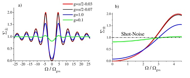
Figure 2: (Color online) Squeezing spectra $\Sigma_{\pm}(\Omega)$ (17), and degree of EPR correlation between the MOPO twin beams, as a function of $\Omega/{\Omega_{\mathrm{gvs}}}$, for $\phi_{s}+\phi_{i}$ fixed as in Eq.(21). $\Delta t=0$.The inset (b) is a detail of the minima.

In this case, the noise passes from below to above the shot noise at $\Omega=\pm{\Omega_{\mathrm{gvs}}}\sqrt{\pi^{2}-g^{2}}$, where ${\rm sinc}{\gamma(\Omega)}$ changes sign. These values can be used to define a bandwidth of squeezing $\Delta\Omega={\Omega_{\mathrm{gvs}}}\sqrt{\pi^{2}-g^{2}}\approx 2.7{\Omega_{\mathrm{gvs}}}$ close to threshold. Some remarks are in order: i) The EPR correlation becomes asymptotically perfect as the MOPO threshold is approached, which can be realized only close to a critical point, because the noise in the quiet quadrature can be suppressed only at the expenses of a diverging level of noise in the orthogonal one. ii) The squeezing remain significant at rather large distances from threshold, $\Sigma_{\pm}(0)\simeq 0.09$ for $g=1$, which is $36\%$ below the MOPO threshold. ii) Excellent levels of squeezing are present in the whole emission bandwidth, that we remind is smaller than ${\Omega_{\mathrm{gvs}}}$Corti et al. (2016). This is in sharp contrast with the single-pass co-propagating geometry, where high squeezing is difficult to observeEto et al. (2008), and the orientation of the squeezing ellipses varies rapidly inside the PDC bandwidthGatti et al. (2017). In contrast, for the MOPO the orientation of the ellipses, defined by $\theta(\pm\Omega)$, remains practically constant inside the bandwidth ${\Omega_{\mathrm{gvs}}}$ [see Eqs.(18)-(20)]. This can be viewed as a consequence of the long (${\tau_{\mathrm{gvs}}}$) and short (${\tau_{\mathrm{gvm}}}$) time scales involved in the counterpropagating geometry.

Fig.3 shows the antisqueezing of the sum or difference modes, which occurs for quadrature phases orthogonal to those in Fig.2. In this case the noise diverges on approaching threshold, which is clearly reminiscent of the critical divergence of the MOPO spectra analysed in Corti et al. (2016). The bandwidth of the antisqueezing spectra shrinks getting close to threshold (Fig.3b), which again reflects the shrinking of the spectra and the critical slowing down of temporal fluctuations close to the MOPO thresholdCorti et al. (2016).

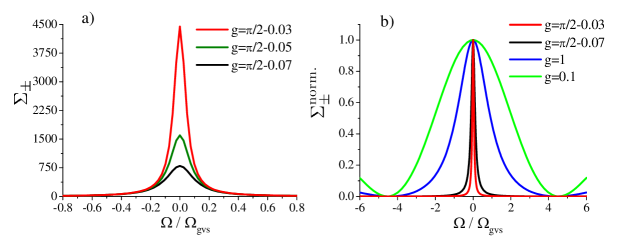
Figure 3: (Color online) Antisqueezing spectra $\Sigma_{\pm}(\Omega)$ (17) as a function of $\Omega/{\Omega_{\mathrm{gvs}}}$, for phase-angles orthogonal to those in Fig.2. The curves in (b) are normalized inside $(0,1)$.

The curves in Figs.2 and 3 are in sense universal for the MOPO, when plotted as a function of $\frac{\Omega}{{\Omega_{\mathrm{gvs}}}}$, and to a very good approximation hold for any material and tuning conditions. This can be more clearly seen by deriving explicit expressions of the noise spectra. By inserting the coefficients(5) in the general result(17), using the linear approximation (8) and neglecting the contribution of the slow phase $\beta(\Omega)$, when $\phi_{s}+\phi_{i}$ is fixed as in Eq.(21), the squeezing spectra can be written as

$$\Sigma_{\pm}^{\text{\tiny{ S}}}(\Omega) =\frac{\sqrt{g^{2}+\tilde{\Omega}^{2}}-g\sin{\sqrt{g^{2}+\tilde{\Omega}^{2}}}}{\sqrt{g^{2}+\tilde{\Omega}^{2}}+g\sin{\sqrt{g^{2}+\tilde{\Omega}^{2}}}}$$ (22)

where $\tilde{\Omega}=\Omega/{\Omega_{\mathrm{gvs}}}$. The antisqueezing spectra, for phases orthogonal to those in Eq.(21), are just the inverse $\Sigma_{\pm}^{A}(\Omega)=1/{\Sigma_{\pm}^{S}(\Omega)}$. This expressions take a particularly simple form in the neighborhood of threshold and for small frequencies. Let us define a distance from threshold $\epsilon=g_{\mathrm{thr}}-g$ and let us consider the limit $\epsilon\ll 1$ and $|\tilde{\Omega}|\ll g$. By expanding the various functions in Eq.(22) around $\epsilon=0$ and $\tilde{\Omega}/g=0$, and keeping terms at most quadratic in the small quantities, we obtain

$$\Sigma_{\pm}^{S}(\Omega)\underset{\begin{subarray}{c}{\epsilon\ll 1}\\ {|\tilde{\Omega}|\ll g}\end{subarray}}{\longrightarrow}\; \frac{1}{4}\left(\epsilon^{2}+\frac{\tilde{\Omega}^{2}}{g_{\mathrm{thr}}^{2}}\right)\,.$$ (23)

This function is a parabola which reaches its minimum at $\Sigma_{\pm}(0)=\frac{\epsilon^{2}}{4}\to 0$ as $\epsilon\to 0$, and of width $\Delta\tilde{\Omega}\approx 2g_{\mathrm{t}hr}$ constant close to threshold. In the same limit, the antisqueezing spectra become

$$\Sigma_{\pm}^{A}(\Omega)\underset{\begin{subarray}{c}{\epsilon\ll 1}\\ {|\tilde{\Omega}|\ll g}\end{subarray}}{\longrightarrow}\; \frac{4}{\epsilon^{2}+\frac{\tilde{\Omega}^{2}}{g_{\mathrm{thr}}^{2}}}$$ (24)

which represents a Lorentzian peak of diverging height $\frac{4}{\epsilon^{2}}\to\infty$ and of vanishing width $\Delta\tilde{\Omega}=\epsilon g_{\mathrm{t}hr}\to 0$, as threshold is approached. These approximated formula nicely reproduce the minima and the maxima in Figs.2 and 3, respectively, when not too far from threshold, and are actually valid for rather large distances from threshold, as shown by Fig.4 .

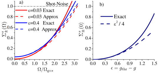
Figure 4: (Color online)Comparison between the exact results in Eq.(17), and the approximated ones in Eq.(23). Squeezing spectra (a) as function of frequency, and (b) at zero frequency as a function of the distance from threshold

.

We notice that such behaviors of the squeezing spectra are completely comparable to what can be obtained in standard cavity OPOs below threshold (see e.g Ref.Walls and Milburn (1994), formula (7.59),page 131). Here, in the degenerate case, the spectrum of squeezing has the form

$$\Sigma^{\mathrm{O}PO}(\Omega) =\frac{(A_{p}^{thr}-A_{p})^{2}+\bar{\Omega}^{2}}{(A_{p}^{thr}+A_{p})^{2}+\bar{\Omega}^{2}}\underset{|\bar{\Omega}|\ll 2}{\to}\frac{1}{4}\left(\epsilon^{2}+\bar{\Omega}^{2}\right)$$ (25)

where $A_{p}$ is a cavity gain parameter, proportional to the pump amplitude, the $\chi^{(2)}$ susceptibility and the photon lifetime in the cavity; $\bar{\Omega}$ is the frequency normalized to the cavity linewidth; the OPO threshold is at $A_{p}=A_{p}^{thr}=1$, and $\epsilon=A_{p}^{thr}-A_{p}$ defines also in the OPO case the dimensionless distance from threshold. Remarkably, in both MOPO and OPO cases, the behavior $\sim\epsilon^{2}/4$ with the distance from threshold indicates that excellent level of squeezing can be obtained even at rather large distances below the threshold.

As a final, we remark that the spectra in Figs.2 and 3 were calculated in the specific case of periodically poled Lithium Niobate ( PPLN), pumped at $800$nm, with $\Lambda=368$ nm, suitable to phase-match the type 0 process at $\lambda_{s}=\lambda_{i}$. The wave-numbers were evaluated using the complete Sellmeier relations in Nikogosi͡an (2005). However, we did not notice appreciable differences (unless at very large frequencies $\Omega\geq 15{\Omega_{\mathrm{gvs}}}$) with the linearly approximated results (22), nor with curves obtained for different materials or tuning conditions, which confirms that our results are completely general for any MOPO configuration.

In conclusions, the MOPO below threshold is a source of EPR entangled beams over a wide range of light frequencies, including telecom wavelengths. Our analysis has shown that this cavityless configuration of PDC can reach the same narrowband, high level, and robust correlation characteristic of the cavity OPO, which represents the golden standard to for EPR beams. As such, it can be used as an alternative to the OPO, meeting the increasing demand for monolithic devices in the field of integrated quantum optics.

References

- Christ et al. (2009) A. Christ, A. Eckstein, P. J. Mosley, and C. Silberhorn, Opt. Expr. 17, 3441 (2009), URL http://www.opticsexpress.org/abstract.cfm?URI=oe-17-5-3441.
- Gatti et al. (2015) A. Gatti, T. Corti, and E. Brambilla, Phys. Rev. A 92, 053809 (2015), URL http://link.aps.org/doi/10.1103/PhysRevA.92.053809.
- Brambilla et al. (2016) E. Brambilla, T. Corti, and A. Gatti, ArXiv e-prints (2016), eprint 1607.06012, URL https://arxiv.org/abs/1607.06012.
- Canalias and Pasiskevicius (2008) C. Canalias and V. Pasiskevicius, Nat. Photon. 1, 459 (2008), URL http://dx.doi.org/10.1038/nphoton.2007.137.
- Corti et al. (2016) T. Corti, E. Brambilla, and A. Gatti, Phys. Rev. A 93, 023837 (2016), URL http://link.aps.org/doi/10.1103/PhysRevA.93.023837.
- Einstein et al. (1935) A. Einstein, B. Podolsky, and N. Rosen, Phys. Rev. 47, 777 (1935), URL http://link.aps.org/doi/10.1103/PhysRev.47.777.
- Reid (1989) M. D. Reid, Phys. Rev. A 40, 913 (1989), URL http://link.aps.org/doi/10.1103/PhysRevA.40.913.
- Ou et al. (1992) Z. Y. Ou, S. F. Pereira, H. J. Kimble, and K. C. Peng, Phys. Rev. Lett. 68, 3663 (1992), URL http://link.aps.org/doi/10.1103/PhysRevLett.68.3663.
- Gerry and Knight (2005) C. C. Gerry and P. L. Knight, Introductory Quantum Optics (2005).
- Lemieux et al. (2016) S. Lemieux, M. Manceau, P. R. Sharapova, O. V. Tikhonova, R. W. Boyd, G. Leuchs, and M. V. Chekhova, Phys. Rev. Lett. 117, 183601 (2016), URL http://link.aps.org/doi/10.1103/PhysRevLett.117.183601.
- La Porta and Slusher (1991) A. La Porta and R. E. Slusher, Phys. Rev. A 44, 2013 (1991), URL https://link.aps.org/doi/10.1103/PhysRevA.44.2013.
- Eto et al. (2008) Y. Eto, T. Tajima, Y. Zhang, and T. Hirano, Opt. Express 16, 10650 (2008), URL http://www.opticsexpress.org/abstract.cfm?URI=oe-16-14-10650.
- Kaiser et al. (2016) F. Kaiser, B. Fedrici, A. Zavatta, V. D’Auria, and S. Tanzilli, Optica 3, 362 (2016), URL http://www.osapublishing.org/optica/abstract.cfm?URI=optica-3-4-362.
- Harris (1966) S. E. Harris, Appl. Phys. Lett. 9, 114 (1966), URL http://scitation.aip.org/content/aip/journal/apl/9/3/10.1063/1.1754668.
- Suhara and Ohno (2010) T. Suhara and M. Ohno, IEEE Journal of Quantum Electronics 46, 1739 (2010).
- Ding and Khurgin (1996) Y. Ding and J. Khurgin, Quantum Electronics, IEEE Journal of 32, 1574 (1996), ISSN 0018-9197.
- Gatti et al. (2017) A. Gatti, T. Corti, and E. Brambilla (2017), in preparation.
- Walls and Milburn (1994) D. Walls and G. Milburn, Quantum Optics (1994).
- Nikogosi͡an (2005) D. Nikogosi͡an, Nonlinear Optical Crystals: A Complete Survey (Springer, 2005), ISBN 9780387220222, URL https://books.google.it/books?id=ZW9Ynx_Z7kkC.