Evolution of coexisting long and short period stellar activity cycles

Abstract

The magnetic activity of the Sun becomes stronger and weaker over roughly an 11 year cycle, modulating the radiation and charged particle environment experienced by the Earth as “space weather.” Decades of observations from the Mount Wilson Observatory have revealed that other stars also show regular activity cycles in their Ca ii H+K line emission, and identified two different relationships between the length of the cycle and the rotation rate of the star. Recent observations at higher cadence have allowed the discovery of shorter cycles with periods between $1$–$3\,{\rm yr}$. Some of these shorter cycles coexist with longer cycle periods, suggesting that two underlying dynamos can operate simultaneously. We combine these new observations with previous data, and we show that the longer and shorter cycle periods agree remarkably well with those expected from an earlier analysis based on the mean activity level and the rotation period. The relative turbulent length scales associated with the two branches of cyclic behavior suggest that a near-surface dynamo may be the dominant mechanism that drives cycles in more active stars, whereas a dynamo operating in deeper layers may dominate in less active stars. However, several examples of equally prominent long and short cycles have been found at all levels of activity of stars younger than $2.3\,{\rm Gyr}$. Deviations from the expected cycle periods show no dependence on the depth of the convection zone or on the metallicity. For some stars that exhibit longer cycles, we compute the periods of shorter cycles that might be detected with future high-cadence observations.

1. Introduction

Activity cycles akin to the 11 year sunspot cycle have been seen for many late-type stars in their Ca ii H+K line emission, since Wilson (1963, 1968, 1978) initiated their systematic study half a century ago. This emission is a proxy of chromospheric activity (Eberhard & Schwarzschild, 1913). The Ca ii H+K flux, normalized by the bolometric flux, is denoted by $R_{\rm HK}$. The chromospheric contribution, denoted by $R^{\prime}_{\rm HK}$, is approximately proportional to the square root of the mean magnetic field strength at the stellar surface (Schrijver et al., 1989). Noyes (1983) showed that the time-averaged value, $\langle R^{\prime}_{\rm HK}\rangle$, is proportional to the inverse Rossby number, $\tau/P_{\rm rot}$, where $\tau$ is the turnover time obtained from stellar mixing length models and $P_{\rm rot}$ is the stellar rotation period. For large values of $\tau/P_{\rm rot}$, the star’s activity saturates at $\log\langle R^{\prime}_{\rm HK}\rangle\approx-4.2$ (Noyes et al., 1984a), which is interpreted in terms of starspots having filled the entire surface of the star (Saar & Linsky, 1985). The time trace of $R^{\prime}_{\rm HK}$ varies with the activity cycle, revealing its cycle period $P_{\rm cyc}$. However, it is affected by flares and the presence of spots. The relative cycle amplitude can be determined as $A_{\rm cyc}=\Delta R^{\prime}_{\rm HK}/R^{\prime}_{\rm HK}\equiv\Delta\ln R^{\prime}_{\rm HK}$. The time trace can also be used to infer $P_{\rm rot}$. Understanding the dependence of these quantities on other stellar properties is an important goal of stellar dynamo theory.

The work of Noyes et al. (1984b) showed that, for G and K dwarfs with $\tau$ between 11 and 26 days and $P_{\rm rot}$ between 22 and 48 days, $1/P_{\rm cyc}$ scales with $\tau/P_{\rm rot}$ as

$$1/P_{\rm cyc}\propto(\tau/P_{\rm rot})^{n},$$ (1)

where $n=1.25$. Kleeorin et al. (1983) theoretically studied two types of stellar dynamos: one with overlapping induction layers (as in the early work of Parker, 1955) and one with non-overlapping ones (as in the spherical shell models of Steenbeck & Krause, 1969). They found that, in the former case of overlapping induction layers, the cycle period of the fastest growing mode obeys $n=4/3$, which is close to the observed value. Later, using nonlinear, plane-wave dynamo models, Robinson & Durney (1982) found $n<1$ for different nonlinearities, which was in conflict with the observations. In a subsequent review, Baliunas & Vaughan (1985) showed that there are many more stars that do not obey any relation between $P_{\rm cyc}$ and $P_{\rm rot}$. However, this view has changed considerably in subsequent years.

A major difficulty lies in the fact that, when comparing stars of different spectral type, one has to rely on a meaningful determination of $\tau$, which is a model-dependent quantity. Noyes et al. (1984a) computed $\tau$ as the ratio of the mixing length to the turbulent velocity approximately one scale height above the bottom of the convection zone. The relevance of such a definition is unclear, given that the location of the dynamo is still not known. Parker (1975) assumed it to operate at the bottom of the convection zone, whereas Brandenburg (2005) argued in favor of a dynamo distributed throughout the convection zone, but with the near-surface shear layer playing an important role in producing the observed equatorward migration of the toroidal flux belts; see corresponding models by Pipin & Kosovichev (2011). Flux transport dynamos (Choudhuri et al., 1995; Dikpati & Charbonneau, 1999), on the other hand, are intermediate in the sense that the toroidal field resides mostly at the bottom of the convection zone, and is the result of shearing a poloidal field that is sourced by the tilt of decaying active regions at the surface. Thus, it has non-overlapping induction layers, as in Steenbeck & Krause (1969), but with meridional circulation playing an important role in determining cycle period and migration direction of the toroidal flux belts. The resulting cycle period then decreases with increasing rotation period with $n\approx-0.25$, which has the wrong sign (Jouve et al., 2010; Karak et al., 2014).

To avoid the dependence on $\tau$ in the interpretation of stellar cycle data, Tuominen et al. (1988) considered the ratio $P_{\rm cyc}/P_{\rm rot}$, which they found to decrease systematically with increasing thickness of the convection zone. Following a similar idea, Soon et al. (1993) plotted this ratio versus age and color $B-V$, whereas Brandenburg et al. (1998) (hereafter BST) plotted it versus both $\langle R^{\prime}_{\rm HK}\rangle$ (hereafter BST diagram) and $\tau/P_{\rm rot}$. These papers used a subset of the extended data set from the Mount Wilson HK project (Baliunas et al., 1995). Owing to the proportionality between $\langle R^{\prime}_{\rm HK}\rangle$ and $\tau/P_{\rm rot}$, both graphs are similar and show two branches with positive slopes, $\nu_{\rm A}$ and $\nu_{\rm I}$. The subscripts A and I for active and inactive refer to the two groups of stars in a previously identified bimodal distribution as a function of $\langle R^{\prime}_{\rm HK}\rangle$ with a local minimum at $\log\langle R^{\prime}_{\rm HK}\rangle\approx-4.75$, which is known as the Vaughan–Preston gap (Vaughan & Preston, 1980).

The question of which quantities to plot against each other is of considerable importance to the present paper. The sensitivity to a model-dependent definition of the turnover time is obviously alleviated when plotting just $P_{\rm cyc}$ against $P_{\rm rot}$, as done by Böhm-Vitense (2007) (hereafter BV), referred to below as the BV diagram. In such a representation, the same two branches are recovered, suggesting a basic equivalence between the BV and BST diagrams. However, in the BV diagram, the Sun appears between the two branches, whereas it is closer to the inactive branch in the BST diagram. The idea that the Sun takes a special position (in one of the two representations) has received much interest and deserves a renewed look.

Because $R^{\prime}_{\rm HK}$ and $\tau/P_{\rm rot}$ are proportional to each other and since $R^{\prime}_{\rm HK}$ is often not available (Saar & Brandenburg, 1999), the representation of the period ratio over $\tau/P_{\rm rot}$ has become popular. However, in comparison with the BV representation, it suffers from the shortcoming that it now involves the model-dependent and ill-determined turnover time. It is therefore important to remind the reader that this criticism does not apply to the original BST diagram, which does not use $\tau/P_{\rm rot}$, but instead $R^{\prime}_{\rm HK}$, which is an observational quantity – independent of stellar models.

An important difference between the BST and BV diagrams lies in the fact that the BST diagram takes into account the dependence on another parameter, namely $\langle R^{\prime}_{\rm HK}\rangle$. Using the linear representation of $P_{\rm cyc}$ versus $P_{\rm rot}$, BV found that the two are proportional to each other, but with different slopes. In other words, their ratio $P_{\rm cyc}/P_{\rm rot}$ is constant on each of the two branches. If this were strictly true, the branches in the BST diagram should be horizontal, so the slopes $\nu_{\rm I}$ and $\nu_{\rm A}$ would vanish. This does not seem to be the case, however, and the new data points discussed in this paper confirm this. Indeed, a linear fit in the BV representation implies $n=1$ in Equation (1), whereas Noyes et al. (1984b) found $n=1.25$.

The graph of $P_{\rm rot}/P_{\rm cyc}$ versus $\langle R^{\prime}_{\rm HK}\rangle$ has a theoretical interpretation in terms of mean-field dynamo theory. For this discussion, it is useful to define the cycle and rotation frequencies, $\omega_{\rm cyc}=2\pi/P_{\rm cyc}$ and $\Omega=2\pi/P_{\rm rot}$, so $\omega_{\rm cyc}/\Omega=P_{\rm rot}/P_{\rm cyc}$. Next, we assume that both the $\alpha$ effect and the radial angular velocity gradient, $\Omega^{\prime}$, are proportional to $\Omega$, and that the $\alpha$ effect depends on the mean magnetic field, $\overline{B}$, via a “quenching function.” For a plane-wave $\alpha\Omega$ dynamo, the cycle frequency is given by (Stix, 1976)

$$\omega_{\rm cyc}\approx|\alpha\Omega^{\prime}|^{1/2}.$$ (2)

Because $R^{\prime}_{\rm HK}$ is approximately proportional to $\overline{B}^{0.5}$ (Schrijver et al., 1989), the graph of $\omega_{\rm cyc}/\Omega$ versus $\langle R^{\prime}_{\rm HK}\rangle$ is a direct representation of the quenching function.

Positive slopes, i.e., positive values of $\nu_{\rm A}$ and $\nu_{\rm I}$ therefore indicate that the $\alpha$ effect is an increasing function of magnetic field strength on these branches. This is referred to as “anti-quenching,” which suggests that the $\alpha$ effect is magnetically driven, and therefore the result of a magnetic instability (Brandenburg & Schmitt, 1998)—not, as usually assumed, driven by flow instabilities such as convection, which would be suppressed with increasing $\overline{B}$. In this model, saturation of the dynamo would be achieved by turbulent diffusion also being an increasing function of magnetic field strength (BST). Explicit evidence for an $\alpha$ effect and a turbulent diffusivity that increase with increasing field strength has been obtained by Chatterjee et al. (2011). For larger field strengths, however, we expect proper quenching with a negative slope, which was confirmed for a group of stars that was referred to as superactive stars (Saar & Brandenburg, 1999).

The topic of stellar cycle frequencies has received increased attention in recent years with new data of high cadence becoming available, allowing the determination of shorter cycle periods (Metcalfe et al., 2010, 2013; Egeland et al., 2015). Spectropolarimetric surveys also led to measuring magnetic fields (Marsden et al., 2014). Furthermore, photometric data collected by missions such as Kepler provided additional activity cycle detections and the measurement of activity levels (e.g. García et al., 2010; García et al., 2014; Mathur et al., 2014; Salabert et al., 2016a). The question of cycle frequencies has become particularly interesting in connection with the recent discovery of reduced magnetic braking of stars whose activity falls below a certain threshold (van Saders et al., 2016). The Sun happens to fall close to this threshold value ($\log\langle R^{\prime}_{\rm HK}\rangle\approx-4.95$), suggesting it therefore to be within a state of transition (Metcalfe et al., 2016). This idea has so far only been discussed in the framework of the BV diagram, in which the Sun takes a prominent position. One of our aims is therefore to clarify the apparent contradiction to the BST diagram. For this purpose, we combine the results from a larger data set, and assess carefully the reliability of all the stars in our sample. Furthermore, we initially consider only K dwarfs, because they tend to have more clearly defined cycle periods. We then study F and G dwarfs—keeping in mind, however, that their cycles tend to be more irregular, and therefore the determination of cycle periods is often less certain. We then discuss individual stars, first those with two cycles, and then inactive and active stars with just one short or one long cycle, respectively. In several cases, we discuss theoretically computed values that would be expected based on our fits. Finally, we consider possible dependencies of the residuals on metallicity, age, or thickness of the convection zone.

2. Analysis of cycle periods

2.1. Sample selection

Out of the 112 stars of Baliunas et al. (1995), BST used a subset of 21 stars. BV excluded HD 219834A, but included 6 additional stars (HD 1835, HD 20630, HD 76151, HD 100180, HD 190406, and HD 165341A), all of which were among the expanded sample of Saar & Brandenburg (1999), who excluded HD 219834A because the cycle period was comparable to the length of the data set. Except for the Sun, the remaining 20 stars of BST were all part of the 50 stars in the original program of Wilson (1978). Plots of the time series and associated short-term Fourier transforms of many of these stars can be found in Olah et al. (2016). In the following, we analyze the cycle periods of 35 stars, which include the 27 stars from Baliunas et al. (1995), two additional stars from their sample (HD 22049 and HD 30495), and two stars observed by the Kepler mission—KIC 10644253 and KIC 8006161 (Salabert et al., 2016a; Kiefer et al., 2017). We also include HD 128620 and HD 128621 (= $\alpha$ Cen A & B, Ayres, 2014), along with the solar analogs HD 146233 (= 18 Sco; Hall et al., 2007b) and HD 17051 ($\iota$ Horologii; Metcalfe et al., 2010).

The sample of Saar & Brandenburg (1999) contains another 30 active and inactive stars from Baliunas et al. (1995) and one more photometric variable, as well as 28 superactive stars with periods up to $60\,{\rm yr}$. Lehtinen et al. (2016) discovered secondary periods in some superactive stars in his sample of 21 additional stars. In the following, however, we restrict ourselves to the reduced sample of active and inactive stars, including those with short periods in the $1$–$3\,{\rm yr}$ range. It should be noted, however, that for a few stars from the CoRoT mission, Ferreira Lopes et al. (2015) claim to have found cycles even shorter than one year, but the data record is too sparse to be reliable. Their detailed study is beyond the scope of the present paper and requires a larger sample, including stars from the Kepler mission; see Reinhold et al. (2017) and Montet et al. (2017) for steps in that direction.

2.2. Representation of and fits to the data

Following BST, we plot $\omega_{\rm cyc}/\Omega$ versus $\langle R^{\prime}_{\rm HK}\rangle$ and determine the parameters to the fit

$$\omega_{\rm cyc}/\Omega=b_{i}\langle R^{\prime}_{\rm HK}\rangle^{\nu_{i}}.$$ (3)

BST found $\nu_{\rm I}=0.85$ for inactive stars and $\nu_{\rm A}=0.72$ for active stars. In Equation (3), the index $i$ stands for I (for inactive) or A (for active). Occasionally, we refer to these fits as short and long period branches, which is more compatible with the notion that inactive and active stars can have both cycle periods coexisting. Below, however, short cycle periods are found to range from $1.5\,{\rm yr}$ to $21\,{\rm yr}$, whereas long ones start already at $5.6\,{\rm yr}$, so the attributes long and short are only relative.

In the case of the Sun, which will be considered in Section 2.5 along with other G dwarfs, the longer period might correspond to the period of the Gleissberg cycle, which is about seven times longer than the basic 11 year solar cycle. This is too long to be determined for other stars with the currently available data sets. However, there are several stars whose basic cycle period is in the $1$–$3\,{\rm yr}$ range. Many of them also have a longer period in the $10$–$20\,{\rm yr}$ range. These fit well onto the two lines in the BST diagram.

For each of the two branches, the values of $b_{i}$ are non-intuitive, because they correspond to the value of $\omega_{\rm cyc}/\Omega$ for $\log R^{\prime}_{\rm HK}=0$, which is far away from realistic values. Therefore, it is not meaningful to compare $b_{i}$, because it varies significantly even for small changes in $\nu_{i}$. Thus, we compute

$$\tilde{b}_{i}=b_{i}R_{\rm HKvp}^{\prime\;\nu_{i}}\;,$$ (4)

which corresponds to the value of $\omega_{\rm cyc}/\Omega$ at the Vaughan–Preston gap at $\log R^{\prime}_{\rm HK}=\log R_{\rm HKvp}^{\prime}=-4.75$. These values are listed in Table LABEL:fitcoefs along with $\nu_{i}$.

BST also consider the dependence of $\omega_{\rm cyc}/\Omega$ on $\tau/P_{\rm rot}$, which is similar to that on $\langle R^{\prime}_{\rm HK}\rangle$, because $\langle R^{\prime}_{\rm HK}\rangle$ is well correlated with $\tau/P_{\rm rot}$ (Noyes, 1983). Within the range of interest for cyclic dynamos, i.e., for $\log\langle R^{\prime}_{\rm HK}\rangle<-4.4$, BST found

$$\langle R^{\prime}_{\rm HK}\rangle=c\,(\tau/P_{\rm rot})^{\mu},$$ (5)

with $\mu=0.99$, independent of which of the two branches the cycle frequencies lie on; see Figure 1(c) of BST. Because $\mu$ is close to unity, we can compute the value of $c$ simply from $\log c=\langle\log\langle R^{\prime}_{\rm HK}\rangle-\log(\tau/P_{\rm rot})\rangle_{\rm sample}\approx-4.631$ for the entire sample of stars.

Based on the possible coexistence of two branches for a given value of $\langle R^{\prime}_{\rm HK}\rangle$, we can compute values of $\omega_{\rm cyc}/\Omega$ that would fall perfectly on either of the two branches. We refer to these as “computed” cycle periods. Departures from those values could be explained by a dependence on additional parameters, such as the depth of the convection zone $d$ normalized by the stellar radius $R$, the metallicity [Fe/H], or the age, which might be affecting the cycle period.

In the present paper, we also compare with the BV diagram. When comparing trends in such diagrams, it is useful to convert the fits in the BST diagram using Equations (3) and (5), i.e.,

$$P_{\rm rot}/P_{\rm cyc}\equiv\omega_{\rm cyc}/\Omega=b_{i}\,\langle R^{\prime}_{\rm HK}\rangle^{\nu_{i}}=C_{i}/P_{\rm rot}^{\mu\nu_{i}},$$ (6)

where we have defined $C_{i}=b_{i}(c\tau^{\mu})^{\nu_{i}}$ and $\tau(B-V)$ is taken from Noyes et al. (1984a), i.e.,

$$\log\tau=\left\{\begin{array}[]{l}1.362-0.166x+0.03x^{2}-5.3x^{3},\;\;x>0,\\ 1.362-0.14x,\quad x<0,\end{array}\right.$$ (7)

with $x=1-(B-V)$. Thus, we have

$$P_{\rm cyc}=P_{\rm rot}^{1+{n_{i}}}/C_{i},$$ (8)

which will be overplotted below in our BV diagrams for $i={\rm A}$ and ${\rm I}$, as well as given values of $\tau$. In Table LABEL:fitcoefs we give the values of $\nu_{i}$ and $\tilde{b}_{i}$ from BST, as well as for our sample of K dwarfs discussed in Section 2.4 and those obtained when including our sample of F and G dwarfs discussed in Section 2.5.

Table 1 Fit coefficients for Equations (3) and (4).

BST K dwarfs F,G dwarfs F,G,K dwarfs $\nu_{\rm I}$     0.85     0.75     0.68     0.45 $\nu_{\rm A}$     0.72     0.95 0.25,  0.32     0.44 $\log\tilde{b}_{\rm I}$ $-1.83$ $-1.85$ $-1.87$ $-1.91$ $\log\tilde{b}_{\rm A}$ $-2.67$ $-2.65$ $-2.67,\;-2.44$ $-2.63$

There are several outliers that have been ignored in the calculation of the fit coefficients given in Table LABEL:fitcoefs. For HD 78366 (blue $g$ symbol) and HD 114710 (blue $j$ symbol), the shorter of the two cycle periods still fall close to the A branch. BV argued that their positions in the plot constitute a third branch, which she called the Ab branch. The situation is similar with the $19.2\,{\rm yr}$ period of HD 128620 (blue $k$ symbol) and the the $12.9\,{\rm yr}$ period of HD 100180 (blue $H$ symbol), both of which would fall on the Ab branch and will be discussed separately in Section 2.5. Therefore, they are not used in the determination of the I or A branches. We return to a detailed discussion of those stars in Section 3, where we argue that the shorter cycle periods close to the A branch are questionable. We also exclude the estimated $80\,{\rm yr}$ period of the solar Gleissberg cycle (blue $A$ symbol) from the fit to the A branch. We emphasize, however, that none of these stars have been excluded from any of the plots.

2.3. Stellar ages

Knowing the star’s age is important when interpreting stellar cycles and especially the simultaneous appearance of two cycle periods. There has been significant progress in determining ages through gyrochronology and asteroseismology. For most of the stars, we have computed their ages from Equations (12)–(14) of Mamajek & Hillenbrand (2008) as

$$t=\left\{P_{\rm rot}/[0.407\,(B-V-0.495)^{0.325}]\right\}^{1.767}.$$ (9)

The age for HD 219834A is assumed to be the same as its cooler companion HD 219834B. We adopted asteroseismic ages for HD 17051 (Vauclair et al., 2008), HD 128620, HD 128621 (Bazot et al., 2012), HD 146233 (Li et al., 2012; Mittag et al., 2016), KIC 8006161, KIC 10644253 (Creevey et al., 2017), HD 186408 and HD 186427 (Metcalfe et al., 2015).

2.4. K dwarfs

In Figure 1, we plot the frequency ratio, $\omega_{\rm cyc}/\Omega$, versus $\langle R^{\prime}_{\rm HK}\rangle$ for our sample of K dwarfs with well-defined cycles. We overplot the fits given by Equation (3) using the coefficients for all F, G, K stars listed in the last column of Table LABEL:fitcoefs. The corresponding cycle periods are denoted by $P_{\rm cyc}^{\rm I}$ and $P_{\rm cyc}^{\rm A}$, depending on which of the two branches they are closest to. The stars are indicated correspondingly by lower- and uppercase symbols.

Most of the K dwarfs seem to form a tight relation around lines that have a somewhat larger slope than to the fits for the full set of F, G, K dwarfs. To quantify this further, we determine a separate fit for K dwarfs, but exclude here HD 22049 (red E/e symbols) on both branches, as well as HD 165341A (red n symbol), HD 149661 (red k symbol), and HD 219834A (red r symbol) on the I branch. The fit parameters are listed in Table LABEL:fitcoefs under K stars, and correspond to lines with larger slopes than for the full set of stars, where the aforementioned stars are not ignored.

Three of our K dwarfs have two cycle periods. The occurrence of two cycle periods is not uncommon and has been reported in a number of earlier papers (see, e.g., Saar & Baliunas, 1992; Soon et al., 1993). When possible, both periods are listed in Table LABEL:Kstars together with other properties of the K dwarfs of our sample. We use the relative cycle amplitudes, $A_{\rm cyc}$, obtained by Saar & Brandenburg (2002), to indicate the range of variation in $R^{\prime}_{\rm HK}$ during the cycle. For $\alpha$ Cen A and B, we compared their X-ray cycles with that of the Sun (Ayres, 2014) and estimated their cycle amplitudes to be approximately three and two times smaller than for the Sun.

The spectroscopic parameters $T_{\rm eff}$ and [Fe/H] in Table LABEL:Kstars are mostly from the Geneva-Copenhagen Survey (Nordström et al., 2004) and Ramírez et al. (2013). However, we obtained values from other sources for HD 201091 and 201092 (Kervella et al., 2008), HD 219834A (Gray et al., 2006), and HD 219834B (Fuhrmann, 2008). For most stars, the activity indexes and cycle periods are from Baliunas et al. (1995). Rotation periods and uncertainties come from Baliunas et al. (1996) and Donahue et al. (1996). Exceptions are discussed in Section 3.

It is instructive to see where the stars shown in Figure 1 are located in the BV diagram. The result is shown in Figure 2. The solid lines show the fits found by BV (hereafter BV lines), whereas the curves correspond to the fit of BST, which has been converted into a $P_{\rm cyc}$ versus $P_{\rm rot}$ dependence using Equation (8) for three values of $\tau$.

Interestingly, in the BV plot, the two cycle periods of HD 22049 (red E/e symbols) do fall onto the two branches. The same is true of HD 165341A (red N/n symbols), where the longer cycle period of $15.5\,{\rm yr}$ agrees well with the computed one (see Table LABEL:Kstars), but the shorter one of $5.1\,{\rm yr}$ is twice as long as the computed one of $2.8\,{\rm yr}$. In the BV plot, on the other hand, this star falls onto the lower (inactive) branch.

The two branches of BST correspond to a bundle of lines in the BV plot, because the conversion from one to the other requires an assumption about the value of $\tau$; see Equation (6) and the definition of $C_{i}$, which involves $\tau$. In the BV plot, the BST lines are not straight, but they would become straight in a double-logarithmic version of this plot. Some of the scatter can be explained by the fact that the K dwarfs have different values of $\tau$.

Table 2 Sample of K dwarfs (red symbols).

Sym HD/KIC Sp $B$–$V$ $T_{\rm eff}$ [Fe/H] $d/R$ $\!\!\log\langle R^{\prime}_{\rm HK}\rangle\!\!$ age $\tau\;$ $P_{\rm rot}$ $P_{\rm cyc}^{\rm I}$ comp $P_{\rm cyc}^{\rm A}$ comp $A_{\rm cyc}^{\rm I}$ $A_{\rm cyc}^{\rm A}$ a      3651 K0 0.84 5128 $0.19$ 0.327 $-4.99$ 7.2 20.6 $44.0$ $13.8\pm 0.4$ 12.6 66.5 0.36 b      4628 K2 0.89 5035 $-0.17$ 0.303 $-4.85$ 5.3 21.7 $38.5\pm 2.1$ $8.6\pm 0.1$ 9.6 50.5 0.38 c   10476 K1 0.84 5188 $-0.04$ 0.317 $-4.91$ 4.9 20.6 $35.2\pm 1.6$ $9.6\pm 0.1$ 9.3 49.1 0.38 d   16160 K3 0.98 4819 $0.08$ 0.326 $-4.96$ 6.9 22.8 $48.0\pm 4.7$ $13.2\pm 0.2$ 13.3 70.1 0.32 e   22049 K2 0.88 5152 $0.00$ 0.319 $-4.46$ 0.6 21.5 $11.1\pm 0.1$ $2.9\pm 0.1$ 1.8 $12.7\pm 0.3$ 9.7 f   26965 K1 0.82 5284 $-0.04$ 0.314 $-4.87$ 7.2 20.1 $43.0$ $10.1\pm 0.1$ 10.9 57.6 0.38 g   32147 K5 1.06 4745 $0.19$ 0.354 $-4.95$ 6.3 23.5 $48.0$ $11.1\pm 0.2$ 13.2 69.4 0.42 h   81809 K0 0.80 5623 $-0.29$ 0.305 $-4.92$ 6.6 19.4 $40.2\pm 3.0$ $8.2\pm 0.1$ 10.7 56.6 i 115404 K1 0.93 5081 $-0.16$ 0.306 $-4.48$ 1.4 22.3 $18.5\pm 1.3$ 3.1 $12.4\pm 0.4$ 16.6 0.16 j 128621 K1 0.88 5230 $0.27$ 0.339 $-4.93$ 5.4 21.5 $36.2\pm 1.4$ $8.1\pm 0.2$ 9.7 51.4 0.11 k 149661 K2 0.80 5199 $-0.01$ 0.302 $-4.58$ 2.1 19.4 $21.1\pm 1.4$ $4.0\pm 0.1$ 4.0 $17.4\pm 0.7$ 21.0 0.35 0.15 l 156026 K5 1.16 4600 $-0.34$ 0.311 $-4.66$ 1.3 24.2 $21.0$ 4.3 $21.0\pm 0.9$ 22.7 0.37 m 160346 K3 0.96 4797 $-0.09$ 0.335 $-4.79$ 4.4 22.7 $36.4\pm 1.2$ $7.0\pm 0.1$ 8.5 45.0 0.44 n    165341A K1 0.78 5023 $-0.29$ 0.307 $-4.55$ 2.0 18.6 $19.9$ $5.1\pm 0.1$ 3.6 $15.5$ 19.1 0.54 0.12 o 166620 K5 0.90 5000 $-0.08$ 0.333 $-4.96$ 6.2 21.9 $42.4\pm 3.7$ $15.8\pm 0.3$ 11.7 61.8 0.30 p 201091 K5 1.18 4400 $-0.20$ 0.338 $-4.76$ 3.3 24.4 $35.4\pm 9.2$ $7.3\pm 0.1$ 8.0 42.4 0.32 q 201092 K7 1.37 4040 $-0.27$ 0.369 $-4.89$ 3.2 25.9 $37.8\pm 7.4$ $11.7\pm 0.4$ 9.8 51.6 0.21 r    219834A K5 0.80 5461 $0.23$ 0.321 $-5.07$ 6.2 19.4 $42.0$ $21.0\pm 1.0$ 13.0 68.5 s    219834B K2 0.91 5136 $0.24$ 0.342 $-4.94$ 6.2 22.1 $43.0$ $10.0\pm 0.2$ 11.7 61.9 0.29

2.5. F and G dwarfs

We now discuss F and G dwarfs listed in Table LABEL:Gstars. Here again, most of the spectroscopic inputs come from the Geneva-Copenhagen Survey (Nordström et al., 2004), whereas the rotation and activity measurements and uncertainties are from Baliunas et al. (1995, 1996) and Donahue et al. (1996). For HD 128620, the data come from Ramírez et al. (2013), Ayres (2014), and Bazot et al. (2007). For the Kepler stars, the spectroscopic parameters were obtained by Buchhave & Latham (2015), and the rotation periods come from García et al. (2014). For KIC 8006161, the activity index and cycle period were measured by Karoff et al. (submitted). For KIC 10644253, the magnetic activity index and cycle measurement were done by Salabert et al. (2016a).

In Figure 3 we plot $\omega_{\rm cyc}/\Omega$ versus $\log\langle R^{\prime}_{\rm HK}\rangle$ for our sample of F and G stars. We compare these data points with the fits given by Equation (3) using the coefficients listed in Table LABEL:fitcoefs. We see that there are now somewhat stronger departures than for the K dwarfs, particularly for low $\langle R^{\prime}_{\rm HK}\rangle$ values. On the other hand, the fraction of active F and G dwarfs is larger than for the sample of K dwarfs. The solar $11\,{\rm yr}$ cycle (blue $a$ symbol) now departs much more from the fit than in the original diagram of BST, where the shorter cycle period of $10\,{\rm yr}$ and a longer rotation period of $26.1\,{\rm d}$ (Baliunas et al., 1995) were used. HD 128620 (blue $k$ symbol) is well below the fit line, but it is also old ($5.4\,{\rm Gyr}$) and extremely inactive compared to all the other inactive stars. It will therefore be interesting to find out whether this departure may be connected with the recent discovery of reduced magnetic braking for sufficiently inactive stars (van Saders et al., 2016; Metcalfe et al., 2016; Metcalfe & van Saders, 2017), which has been associated with the dynamo having become subcritical once the rotation rate drops below a critical rotation rate (Kitchatinov & Nepomnyashchikh, 2017).

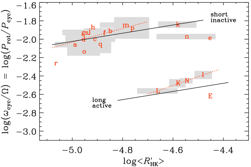
Figure 1.— $\omega_{\rm cyc}^{\rm I}/\Omega$ (lowercase symbols) and $\omega_{\rm cyc}^{\rm A}/\Omega$ (uppercase symbols) versus $\log\langle R^{\prime}_{\rm HK}\rangle$ for the K dwarfs listed in Table LABEL:Kstars. The upper and lower black solid lines come from fits to all F, G, K dwarfs, whereas red dashed lines correspond to fits for K stars only (see text). The gray boxes behind the letters indicate the statistical error in the period ratio and the spread of $\log R^{\prime}_{\rm HK}$ between cycle minimum and maximum.

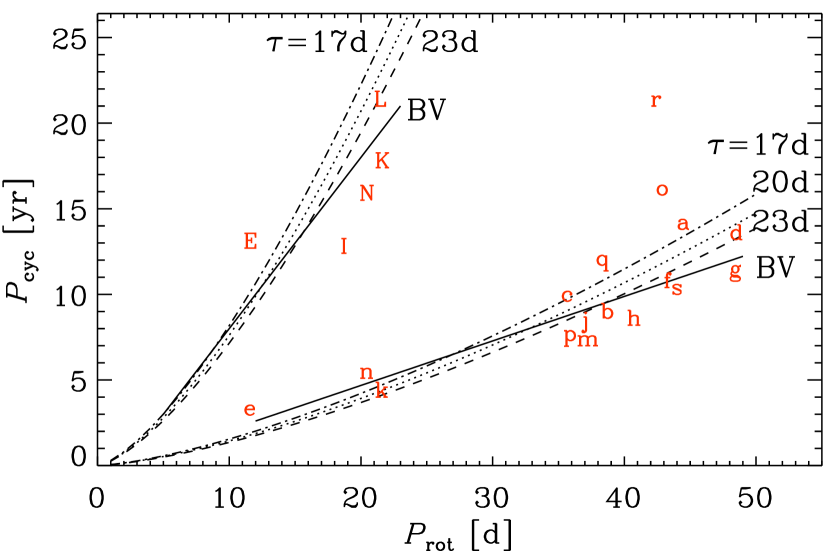
Figure 2.— $P_{\rm cyc}^{\rm I}$ (lowercase symbols) and $P_{\rm cyc}^{\rm A}$ (uppercase symbols) versus $P_{\rm rot}$ for the K dwarfs listed in Table LABEL:Kstars. The dash-dotted, dotted, and dashed lines correspond to $\tau=17\,{\rm d}$, $20\,{\rm d}$, and $23\,{\rm d}$, respectively.

The BV plot for our sample of F and G dwarfs is shown in Figure 4. It has more scatter than the plot for the K dwarfs in Figure 2. However, systematic departures in the BST plot tend to correspond to similar departures in the BV plot. An example is HD 78366, where both the $g$ and $G$ symbols in the BST diagram of Figure 3 are also close to the line for active stars. This is similar for HD 114710, where the $j$ and $J$ symbols are close to the line for active stars. The blue $g$ and $j$ symbols fall along the Ab branch identified by BV. However, the significance of this branch remains uncertain, as will be discussed in Section 3.1. Our fit to this branch shown in Figure 3 (with parameters given in Table LABEL:fitcoefs under F,G stars) also includes the longer cycle periods of HD 20630 (blue $D$ symbol) and HD 100180 (blue $H$ symbol) – in agreement with BV. Interestingly, HD 128620 (blue $k$ symbol) also fits well on this line. The corresponding Aa branch of BV includes the long cycle periods of HD 114710 (blue $J$ symbol) and HD 78366 (blue $G$ symbol), as well as those of HD 190406 (blue $N$ symbol), HD 30495 (blue $E$ symbol), HD 152391 (blue $M$ symbol), and HD 1835 (blue $B$ symbol). Next, we combine the data points of the Aa and Ab branches with those of the long cycle periods of K dwarfs, which lie in between the Aa and Ab branches; see the coefficients in Table LABEL:fitcoefs under F,G,K dwarfs, This was shown as the lower solid lines of Figures 1 and 3. The combined BST diagram is shown in Figure 5 and will be discussed in detail in Section 3.

Table 3 Sample of F and G dwarfs (blue symbols).

Sym HD/KIC Sp $B$–$V$ $T_{\rm eff}$ [Fe/H] $d/R$ $\!\!\log\langle R^{\prime}_{\rm HK}\rangle\!\!$ age $\tau\;$ $P_{\rm rot}$ $P_{\rm cyc}^{\rm I}$ comp $P_{\rm cyc}^{\rm A}$ comp $A_{\rm cyc}^{\rm I}$ $A_{\rm cyc}^{\rm A}$ a Sun G2 0.66 5778 $0.00$ 0.292 $-4.90$ 4.6 12.6 $25.4\pm 1.0$ $11.0\pm 2.0$ 6.6 $80.0$ 35.0 0.22 b 1835 G3 0.66 5688 $-0.02$ 0.275 $-4.43$ 0.5 12.6 $7.8\pm 0.6$ 1.3 $9.1\pm 0.3$ 6.6 0.15 c 17051 F8 0.57 6053 $0.00$ 0.267 $-4.60$ 0.6 7.5 $8.5\pm 0.1$ $1.6$ 1.6 8.6 d 20630 G5 0.66 5701 $0.00$ 0.292 $-4.42$ 0.7 12.6 $9.2\pm 0.3$ 1.5 $5.6\pm 0.1$ 7.8 0.14 e 30495 G1 0.63 5780 $-0.08$ 0.263 $-4.49$ 1.1 10.9 $11.4\pm 0.2$ $1.7\pm 0.3$ 2.0 $12.2\pm 3.0$ 10.3 f 76151 G3 0.67 5675 $-0.04$ 0.301 $-4.66$ 1.6 13.2 $15.0$ $2.5\pm 0.1$ 3.1 16.1 0.16 g 78366 G0 0.63 5915 $-0.10$ 0.322 $-4.61$ 0.8 10.9 $9.7\pm 0.6$ $5.9\pm 0.1$ 1.9 $12.2\pm 0.4$ 9.9 0.19 0.27 h 100180 F7 0.57 5942 $-0.15$ 0.221 $-4.92$ 2.3 7.5 $14.0$ $3.6\pm 0.1$ 3.7 $12.9\pm 0.5$ 19.7 0.07 0.17 i 103095 G8 0.75 5035 $-1.36$ 0.096 $-4.90$ 4.6 17.4 $31.0$ $7.3\pm 0.1$ 8.1 42.5 0.27 j 114710 F9 0.58 5970 $-0.06$ 0.278 $-4.75$ 1.7 8.0 $12.3\pm 1.1$ $9.6\pm 0.3$ 2.8 $16.6\pm 0.6$ 14.5 0.12 0.21 k 128620 G2 0.71 5809 $0.23$ 0.320 $-5.00$ 5.4 15.4 $22.5\pm 5.9$ $19.2\pm 0.7$ 6.5 34.3 0.07 l 146233 G5 0.65 5767 $-0.02$ 0.268 $-4.93$ 4.1 12.0 $22.7\pm 0.5$ $7.1$ 6.1 32.2 m 152391 G7 0.76 5420 $-0.08$ 0.325 $-4.45$ 0.8 17.8 $11.4\pm 1.4$ 1.9 $10.9\pm 0.2$ 9.9 0.28 n 190406 G1 0.61 5847 $-0.12$ 0.241 $-4.80$ 1.8 9.7 $13.9\pm 1.5$ $2.6\pm 0.1$ 3.3 $16.9\pm 0.8$ 17.3 0.15 0.34 o 8006161 G8 0.84 5488 $0.34$ 0.359 $-5.00$ 4.6 20.6 $29.8\pm 3.1$ $7.4\pm 1.2$ 8.6 45.3 p 10644253 G0 0.59 6045 $0.06$ 0.274 $-4.69$ 0.9 8.6 $10.9\pm 0.9$ $1.5\pm 0.1$ 2.3 12.1 q 186408 G2 0.64 5741 $0.05$ 0.278 $-5.10$ 7.0 11.5 $23.8\pm 1.7$ 7.6 40.2 r 186427 G3 0.66 5701 $0.05$ 0.291 $-5.08$ 7.0 12.6 $23.2\pm 3.2$ 7.3 38.4

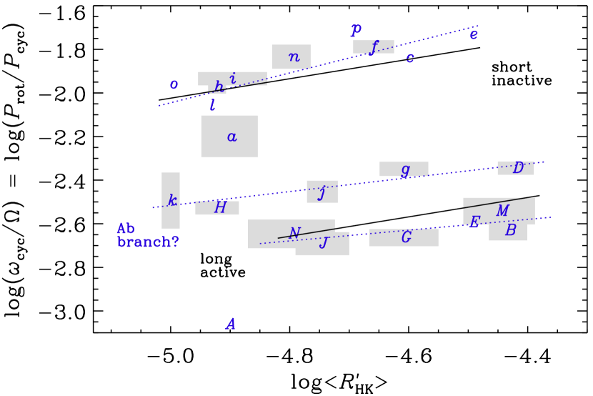
Figure 3.— BST diagram for the F and G dwarfs listed in Table LABEL:Gstars. The black solid lines refer to our fits to F, G, and K stars discussed in the text (and also shown in Figure 1) whereas the upper blue dotted line denotes the fit to the F and G stars. The two lower blue dotted lines denote what corresponds to the Aa and Ab branches in BV, which are here evaluated as fits through N, J, G, E, M, and B on the one hand, and j and g together with D and H, on the other. Otherwise like Figure 1.

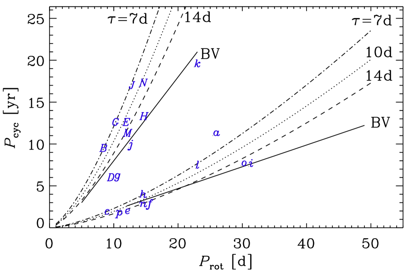
Figure 4.— BV diagram for the F and G dwarfs listed in Table LABEL:Gstars. Otherwise like Figure 2.

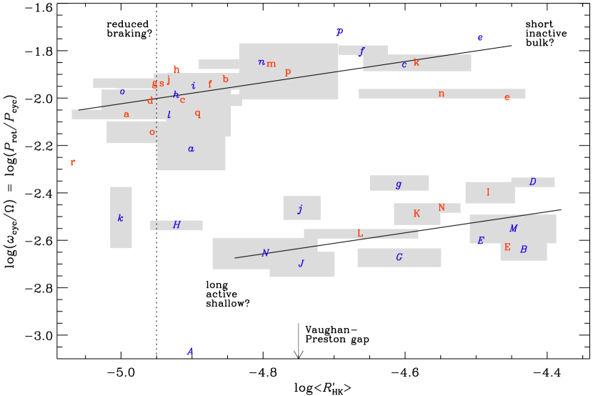
Figure 5.— BST diagram for the F, G, and K dwarfs showing $\omega_{\rm cyc}^{\rm I}/\Omega$ (lowercase symbols) and $\omega_{\rm cyc}^{\rm A}/\Omega$ (uppercase symbols) versus $\log\langle R^{\prime}_{\rm HK}\rangle$ for the K dwarfs (red roman symbols) listed in Table LABEL:Kstars and F and G dwarfs (blue italics symbols) listed in Table LABEL:Gstars. The upper and lower solid lines correspond to fits to the groups of short and long cycle periods on the branches of inactive and active stars, respectively. The gray boxes behind the letters indicate the statistical error in the period ratio and the spread of $\log R^{\prime}_{\rm HK}$ between cycle minimum and maximum. The vertical dotted line at $\log R^{\prime}_{\rm HK}=-4.95$ corresponds to $P_{\rm rot}/\tau\approx 2.1$, which van Saders et al. (2016) identified as the position beyond which magnetic braking is reduced. The Vaughan–Preston gap at $\log R^{\prime}_{\rm HK}=-4.75$ is marked by an arrow.

3. Discussion of individual stars

We now discuss individual stars, referring to their red roman symbols for K dwarfs and blue italics symbols for F and G dwarfs in Figure 5. We frequently compare the observed cycle periods with the computed ones.

Table 4Stars with double periods and their ages.

F dwarfs G dwarfs K dwarfs (HD 17051) ($0.6\,{\rm Gyr}$) HD 78366 ($0.8\,{\rm Gyr}$) HD 22049 ($0.6\,{\rm Gyr}$) HD 114710 ($1.7\,{\rm Gyr}$) HD 30495 ($1.1\,{\rm Gyr}$) HD 165341A ($2.0\,{\rm Gyr}$) HD 100180 ($2.3\,{\rm Gyr}$) (HD 76151) ($1.6\,{\rm Gyr}$) HD 149661 ($2.1\,{\rm Gyr}$) HD 190406 ($1.8\,{\rm Gyr}$)

3.1. Stars with two cycle periods

Looking at Tables LABEL:Kstars and LABEL:Gstars, there are eight cases of stars with double periods (three K dwarfs, four G dwarfs, and two F dwarfs). In addition, we discuss the F dwarf HD 17051 ($\iota$ Hor) and the G dwarf HD 76151, for which longer cycle periods have tentatively been detected. The ages of these ten stars are between $0.6$ and $2.3\,{\rm Gyr}$; see Table LABEL:DoubleCycles. We begin by discussing first the G dwarfs, where the phenomenon of two periods is particularly striking.

HD 78366 (blue $G/g$ symbols) is a young ($0.8\,{\rm Gyr}$) active G0V star with $\log\langle R^{\prime}_{\rm HK}\rangle\approx-4.42$. It has a longer period of $12.2\,{\rm yr}$ (good), which is close to the computed value of $9.9\,{\rm yr}$ for the active branch, but the shorter one of $5.9\,{\rm yr}$ (fair) is much longer than the computed value of $1.9\,{\rm yr}$. The evidence for the shorter $5.9\,{\rm yr}$ period hinges on two pronounced “spikes” in the time series at times when the longer cycle is close to minimum. The periodogram of Egeland (2017) shows a peak at $5.9\,{\rm yr}$ and also one at $19.8\,{\rm yr}$. However, using Zeeman Doppler Imaging, Morgenthaler et al. (2011) found two reversals between 2008 and 2011, which would be compatible with our computed cycle period of $1.9\,{\rm yr}$. They also quoted a slightly longer rotation period of $11.4\,{\rm d}$ instead of $9.7\,{\rm d}$. This would move the longer cycle period (blue $G$ symbol) even closer to the A branch. This star from the Mount Wilson HK project is also being monitored with the Solar-Stellar Spectrograph (SSS) at Lowell Observatory. Looking at Figure 3, there is some similarity to HD 114710 (blue $J/j$ symbols); in both cases, the shorter period is just one half of the longer one, so these data points are still close to the active branch.

HD 30495 (= 58 Eri, blue $E/e$ symbols), is a young ($1.1\,{\rm Gyr}$) variable G1V star of BY Draconis type, and is considered a solar analog. No cycle periods were given by Baliunas et al. (1995), and only recently did Egeland et al. (2015) discover a short cycle period of $1.67\,{\rm yr}$ and a long one of $12.2\,{\rm yr}$. Both values agree well with the computed ones of $2.0$ and $10.3\,{\rm yr}$, respectively. Although the longer cycle period is apparent in the more recent time trace of Hall et al. (2007a), the shorter one is not so clear owing to poor cadence. With $\log\langle R^{\prime}_{\rm HK}\rangle\approx-4.49$, this star is well above the Vaughan–Preston gap.

HD 190406 (= 15 Sge, blue $N/n$ symbols) is a solar analog with an age of $2.3\,{\rm Gyr}$ and two cycle periods. It is similar to HD 30495, except that it is below the Vaughan–Preston gap and has $\log\langle R^{\prime}_{\rm HK}\rangle\approx-4.80$. Baliunas et al. (1995) determined a short cycle of $2.6\,{\rm yr}$ (fair) and a long one of $16.9\,{\rm yr}$ (good). Both values agree well with the computed periods of $3.3\,{\rm yr}$ and $17.3\,{\rm yr}$, respectively. Egeland (2017) found $1.6$, $2.6$, and $18.7\,{\rm yr}$ from his periodograms. The shorter cycle period is also seen in the more recent observations by Hall et al. (2007a). The short-term Fourier transforms of Olah et al. (2016) clearly show power for both periods, but with different strengths at different times.

HD 114710 (= $\beta$ Com, blue $J/j$ symbols) is an F9V star ($1.7\,{\rm Gyr}$) with two cycle periods that were determined by Baliunas et al. (1995) to be $9.6\,{\rm yr}$ (fair) and $16.6\,{\rm yr}$ (good). With $\log\langle R^{\prime}_{\rm HK}\rangle\approx-4.75$ it is in the Vaughan–Preston gap. The computed periods are $2.8\,{\rm yr}$ and $14.5\,{\rm yr}$, respectively. Although the longer period is close to the computed one, the shorter one is much longer. However, looking at the time trace in Baliunas et al. (1995), the observational cadence is insufficient to discern short periods in the $2$–$3\,{\rm yr}$ range. Therefore, it is conceivable that the shorter period of HD 114710 might not have been determined correctly. Egeland (2017) did find shorter periods of $5.1$ and $6.5\,{\rm yr}$ in his periodograms. This star from the Mount Wilson HK project continues to be monitored with the SSS, thereby also allowing better verification also of the longer cycle period in the future.

HD 100180 (= 88 Leo, blue $H/h$ symbols) is an inactive ($\log\langle R^{\prime}_{\rm HK}\rangle\approx-4.92$) F5V star ($2.3\,{\rm Gyr}$) with two cycle periods that Baliunas et al. (1995) determined to be $3.6\,{\rm yr}$ (fair) and $12.6\,{\rm yr}$ (fair). In this case, the shorter period agrees well with the computed one of $3.7\,{\rm yr}$, but the longer one turns out to be $19.7\,{\rm yr}$. However, given that the time series covered only 25 years, we cannot exclude that the actual period was longer. This impression is confirmed by direct inspection of the time series; see Olah et al. (2016), who quote $16.6$–$9.85\,{\rm yr}$ for the range of the longer cycle period.

HD 22049 (= $\epsilon$ Eri, red E/e symbols) is a very young ($0.6\,{\rm Gyr}$) and active ($\log\langle R^{\prime}_{\rm HK}\rangle\approx-4.46$) K2 star, whose computed cycle periods of $1.8\,{\rm yr}$ and $9.7\,{\rm yr}$ are a bit shorter than the observed ones of $2.9\,{\rm yr}$ and $12.7\,{\rm yr}$ (Metcalfe et al., 2013).

HD 165341A (= 70 Oph A, red N/n symbols) is an active ($\log\langle R^{\prime}_{\rm HK}\rangle\approx-4.55$) K1V star with an age of $2.0\,{\rm Gyr}$, whose longer cycle period of $15.5\,{\rm yr}$ is a bit shorter than the computed one of $19.1\,{\rm yr}$, whereas the shorter one of $5.1\,{\rm yr}$ is longer than the computed $3.6\,{\rm yr}$ period.

HD 149661 (red k/K symbols) is an active ($\log\langle R^{\prime}_{\rm HK}\rangle\approx-4.58$) K2V star with an age of $2.1\,{\rm Gyr}$. The longer of the two periods is $17.4\,{\rm yr}$, which is again a bit shorter than the computed value of $21\,{\rm yr}$. We note in passing that Saar & Brandenburg (1999) quoted a cycle period of $16.2\,{\rm yr}$. The shorter period of $4\,{\rm yr}$ agrees with the computed value. The monitoring of this star is being continued with the SSS.

HD 17051 (= $\iota$ Hor, blue $c$ symbol) is a young ($0.6\,{\rm Gyr}$) F8V star with one of the shortest cycle periods ever detected ($1.6\,{\rm yr}$; Metcalfe et al., 2010). This agrees with the computed value. In Table LABEL:Gstars it is listed with a single period (which is why it is listed in parentheses in Table LABEL:DoubleCycles), but recent evidence now suggests the presence of a longer cycle of $\sim 5\,{\rm yr}$ as well (Flores et al., 2017). The computed value is $8.6\,{\rm yr}$. Strengthening the evidence for the existence of this longer cycle period should be an important goal for future observations.

For the Sun (blue $a$ symbol), we have adopted a cycle period of $11\,{\rm yr}$ instead of the $10\,{\rm yr}$ that was determined by Baliunas et al. (1995) from their limited $\langle R^{\prime}_{\rm HK}\rangle$ time series. As secondary period (blue $A$ symbol), we took an estimated $80\,{\rm yr}$ Gleissberg cycle period. The computed value is only about half as long. However, the Sun is much older than the other stars with double periods, so the $80\,{\rm yr}$ Gleissberg period may not be a proper secondary cycle in the same sense.

3.2. Stars with only a short cycle

We consider stars whose frequency ratios $\omega_{\rm cyc}/\Omega$ are close to those on the inactive or short cycle branch. The $\langle R^{\prime}_{\rm HK}\rangle$ values are mostly below the Vaughan–Preston gap and older than $3\,{\rm Gyr}$. Exceptions are HD 76151 ($1.6\,{\rm Gyr}$) and KIC 10644253 ($0.9\,{\rm Gyr}$), with ages for which there are many stars with longer cycles (Section 3.1). For HD 76151, Egeland (2017) reported a $20.9\,{\rm yr}$ period, which is close to the computed value of $16.1\,{\rm yr}$, but for KIC 10644253, the observations are not long enough to confirm a longer period. In Table LABEL:DoubleCycles, HD 76151 has been listed in parentheses.

HD 201091 (= 61 Cyg A, red p symbol) is an inactive K5V star ($3.3\,{\rm Gyr}$) with a $7.3\,{\rm yr}$ cycle period that agrees with the computed value of $8\,{\rm yr}$. Its surface field geometry has been assessed using Zeeman Doppler Imaging and is found to be solar-like (Boro Saikia et al., 2016). There is no evidence for a long-term cycle.

HD 10476 (= 107 Psc, red c symbol) is a K1V star ($4.9\,{\rm Gyr}$) with a $9.6\,{\rm yr}$ cycle period – in agreement with the computed $9.3\,{\rm yr}$ period. We note in passing that the rotation period used here is $35.2\,{\rm d}$, as given in BST and Saar & Brandenburg (1999), but BV listed $38.2\,{\rm d}$, which may have been a typo.

HD 81809 (red h symbol) is an old ($6.6\,{\rm Gyr}$) and inactive star with only one period, which is a bit shorter ($8.2\,{\rm yr}$) than the computed one of $10.7\,{\rm yr}$. Baliunas et al. (1995) classified it as a solar-like G2V star with $B-V=0.64$, but suggested that the dominant component of this binary might be a K0V dwarf, for which BST used $B-V=0.80$. In fact, with $B-V=0.64$, the value of $\tau$ would be too small and Equation (5) would result in a value of $\langle R^{\prime}_{\rm HK}\rangle$ that is too small, compared to the actual one. Egeland (2017) also quotes $B-V=0.64$ for the dominant component.

HD 128620 (= $\alpha$ Cen A, blue $k$ symbol) is an old ($5.4\,{\rm Gyr}$) G2V star in the southern hemisphere, and was therefore not included in the original sample of Baliunas et al. (1995). It has one of the most extensive records in the X-ray (Ayres, 2014) as well as in the far ultraviolet (Ayres, 2015) wavelengths. Its cycle period of $19.2\,{\rm yr}$ is slightly closer to the $34\,{\rm yr}$ period computed for the A branch than the $6.5\,{\rm yr}$ value for the I branch. As will be discussed in Section 4.2, its estimated $\langle R^{\prime}_{\rm HK}\rangle$ value of $-5.00$ is $0.2$ dex smaller than expected, based on its rotation period. Neither circular nor linear polarization has been detected, indicating the absence of a net longitudinal magnetic field stronger than $0.2\,{\rm G}$ (Kochukhov et al., 2011). It is fairly metal-rich, with [Fe/H]=0.23.

HD 128621 (= $\alpha$ Cen B, red j symbol) is a K1V star (also $5.4\,{\rm Gyr}$, but with [Fe/H]=0.27). It is about 0.1 dex above the I branch in Figure 5 and its cycle period of $8.1\,{\rm yr}$ is slightly below the computed one of $9.7\,{\rm yr}$.

HD 201092 (red p symbol) with $B-V=1.37$ is the coolest K dwarf ($3.2\,{\rm Gyr}$) in our sample. Its primary cycle period of $11.7\,{\rm yr}$ is close to the computed value of $8\,{\rm yr}$.

HD 219834A (= 94 Aqr, red r symbol) is the least active cycling star in our sample ($\log R^{\prime}_{\rm HK}=-5.07$). Baliunas et al. (1995) classified it as K5V dwarf, but Santos et al. (2010) determined it to be a G6/G8IV subgiant. Its age is $6.4\,{\rm Gyr}$ and its cycle period of $21\,{\rm yr}$ exceeds the computed value of $13\,{\rm yr}$. At this low activity level, one expects reduced magnetic braking to have set in (Metcalfe et al., 2016), which could be responsible for departures from the computed value. This is expected to occur at a critical value of $P_{\rm rot}/\tau\approx 2.1$ (van Saders et al., 2016), which, using Equation (5), corresponds to $\log R^{\prime}_{\rm HK}=-4.95$. This value is marked in Figure 5 by a vertical dotted line.

HD 103095 (blue $i$ symbol) is an extremely metal-poor G8V star ($4.6\,{\rm Gyr}$) with ${\rm[Fe/H]}=-1.36$. The cycle period of $7.3\,{\rm yr}$ agrees well with the computed one of $8.1\,{\rm yr}$.

HD 76151 (blue $f$ symbol) is an active ($\log R^{\prime}_{\rm HK}=-4.66$) G3V star ($1.6\,{\rm Gyr}$) with only a short cycle period of $2.5\,{\rm yr}$. This agrees with the computed one of $3.1\,{\rm yr}$. A longer period of $16.1\,{\rm yr}$ is computed, which is close to the $20.9\,{\rm yr}$ period found by Egeland (2017), but it was not reported by Baliunas et al. (1995). On the other hand, Egeland (2017) reported a $5.0\,{\rm yr}$ period, but his periodogram also shows a peak at $2.6\,{\rm yr}$.

HD 146233 (= 18 Sco, blue $l$ symbol) is the currently accepted best bright solar twin ($4.1\,{\rm Gyr}$). Its cycle period of $7.1\,{\rm yr}$ (Hall et al., 2007b) agrees well with the computed value of $6.1\,{\rm yr}$. Egeland (2017) found $1.9$, $6.5$, and $13.9\,{\rm yr}$ periods.

HD 166620 (red o symbol) is a slowly rotating inactive K5 dwarf ($6.2\,{\rm Gyr}$) with a cycle period of $15.8\,{\rm yr}$, which is below the computed $11.7\,{\rm yr}$ value. It has $\log\langle R^{\prime}_{\rm HK}\rangle=-4.96$, which is slightly (0.1 dex) below the value expected for its slow rotation period of $42.4\,{\rm d}$. In all other aspects, it is unexceptional; it has a similar age and $\langle R^{\prime}_{\rm HK}\rangle$ value to HD 16160 (red d symbol), which has an even longer rotation period of $48\,{\rm d}$.

KIC 8006161 (= HD 173701, blue $o$ symbol), is a G8V star ($4.6\,{\rm Gyr}$) with a short period of $7.7\,{\rm yr}$, which is somewhat shorter than the computed $8.6\,{\rm yr}$. With [Fe/H] = 0.34, this star has the largest metallicity in our sample.

KIC 10644253 (blue $p$ symbol) is a young ($0.9\,{\rm Gyr}$) solar analog of spectral type G5V (Salabert et al., 2016a), with a $1.5\,{\rm yr}$ cycle period (Salabert et al., 2016b) determined from seismology, which is shorter than the computed period of $2.3\,{\rm yr}$. The computed value for the longer cycle of $12.1\,{\rm yr}$ is not observed, but looking for a longer cycle should be a priority for future observations.

There are several other K dwarfs with single short cycles that are not discussed here in detail: HD 3651, HD 4628, HD 16160, HD 26965, HD 32147, HD 160346, HD 201091, and HD 219834B. In all of these cases, the observed cycle periods are close to the computed values. Their ages are in the range $3.3$–$7.2\,{\rm Gyr}$.

3.3. Stars with only a long cycle

Stars with only a long cycle period lie on the A branch and are in that sense active stars. The stars HD 1835, HD 152391, and HD 20630 are well above the Vaughan–Preston gap with $\log\langle R^{\prime}_{\rm HK}\rangle$ in a narrow range between $-4.45$ and $-4.42$ and have ages from $0.5$ to $0.8\,{\rm Gyr}$. They all have computed cycle periods on the short cycle branch between $0.8$ and $1.4\,{\rm yr}$ that would be interesting to look for in future observing programs.

HD 1835 (blue $b$ symbol) is a young G3V star ($0.5\,{\rm Gyr}$) with a cycle period of $9.1\,{\rm yr}$, which is longer than the computed value of $6.4\,{\rm yr}$ for the active branch. Egeland (2017) found a slightly shorter value of $7.8\,{\rm yr}$ as well as a longer period of $20.8\,{\rm yr}$, which is not, however, computed. Instead, there is a shorter computed cycle period of $0.8\,{\rm yr}$ for the inactive branch, which is not observed.

HD 152391 (blue $m$ symbol) is an active G7V star ($0.8\,{\rm Gyr}$) with one period of $10.9\,{\rm yr}$, which falls on the active branch with a computed value of $9.6\,{\rm yr}$. The shorter period of $1.4\,{\rm yr}$ is not observed. This star from the Mount Wilson HK project is also being monitored with the SSS.

HD 20630 (blue $d$ symbol) is a G5V star ($0.7\,{\rm Gyr}$) with a $5.7\,{\rm yr}$ cycle, which is close to the computed value of $7.5\,{\rm yr}$ for the active branch. The computed shorter cycle period of $1.0\,{\rm yr}$ for the inactive branch is not observed. Egeland (2017) found $5.7$, $14.2$, and $35.8\,{\rm yr}$ periods.

Other stars with only a single long cycle include the K dwarfs HD 115404 and HD 156026, with ages $1.4$ and $1.3\,{\rm Gyr}$, respectively. As can be seen from the 36 year time series analyzed by Olah et al. (2016), a longer time series would be desirable in both cases. Of these stars, however, only HD 115404 continues to be monitored with the SSS.

3.4. Stars without cycles

HD 186408 (= 16 Cyg A, blue $q$ symbol) and HD 186427 (= 16 Cyg B, blue $r$ symbol) are Sun-like dwarfs, but at an age of $7\,{\rm Gyr}$ they have no cycle. Table LABEL:Gstars gives computed cycle periods of $7.6$ and $7.3\,{\rm yr}$ that are meaningless in this case. As we shall discuss later, their $\langle R^{\prime}_{\rm HK}\rangle$ values are smaller than what is expected based on their $\tau/P_{\rm rot}$ values, which is a clear indication that they have experienced reduced magnetic braking (Metcalfe & van Saders, 2017).

4. Dependencies of the residuals on other quantities

Equations (3) and (5) define two distinct residuals:

$$\Delta_{i}=\log(\omega_{\rm cyc}/\Omega)-\log\left(b_{i}\langle R^{\prime}_{\rm HK}\rangle^{\nu_{i}}\right)$$ (10)

with $i={\rm I}$ and $i={\rm A}$ for the inactive and active branches, respectively, and

$$c=\log\langle R^{\prime}_{\rm HK}\rangle-\log(\tau/P_{\rm rot})$$ (11)

for both branches. Both $\Delta_{i}$ and $c$ should be constants, i.e., they should not depend systematically on any quantity unless there are indeed additional dependences; for example, on the depth of the convection zone, the metallicity, or the age. In the following, we consider these possibilities.

4.1. Dependence on convection zone thickness

Tuominen et al. (1988) suspected that $\omega_{\rm cyc}/\Omega$ depends on the depth of the convection zone. This possibility arises because the $\alpha$ effect is proportional to the correlation length $\ell$ of the turbulence with $\alpha\approx\Omega\ell$ times some quenching function, as discussed in the introduction. By parameterizing the differential rotation in terms of the local double-logarithmic derivative, $q\equiv{\rm d}{}\ln\Omega/{\rm d}{}\ln r$, we have $\Omega^{\prime}=q\Omega/r$, where $r$ is the radius, so Equation (2) yields $\omega_{\rm cyc}/\Omega\approx|q\ell/r|^{1/2}$. In the near-surface shear layer of the Sun, we have $q\approx-1$ (Barekat et al., 2014); however, in deeper layers, it is positive and of appreciable amplitude only in the tachocline (Schou et al., 1998). If the turbulence governing the $\alpha$ effect is characterized by giant cells of a size comparable to the depth $d$ of the convection zone, one would expect $\omega_{\rm cyc}/\Omega\propto(d/R)^{1/2}$; see Equation (2). Evidence from stellar cycle data was presented in Tuominen et al. (1988), but they ignored the additional dependence on $\langle R^{\prime}_{\rm HK}\rangle$. Therefore, one should consider the dependence of the residual $\Delta_{i}$ on $d/R$.

As a very preliminary measure of $d/R$, let us first look at the dependence of $\Delta_{i}$ on $B-V$; see Figure 6. It is immediately evident that the scatter is much larger for F and G dwarfs on the left. For $B-V>0.9$, the scatter is significantly smaller. This justifies our approach of considering the K dwarfs separately at first instance. Other than that, no systematic dependence on $B-V$ is found.

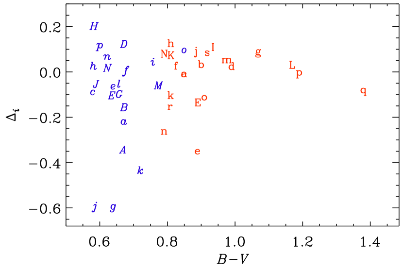
Figure 6.— The residual $\Delta_{i}$ versus $B-V$ for the K dwarfs (red symbols) listed in Table LABEL:Kstars, and the F and G dwarfs (blue symbols) listed in Table LABEL:Gstars. Note the increase of scatter for small values of $B-V$.

Next, we compute the depth of the convection zone for all of the stars with a metallicity measurement. From $B-V$, we compute the mass using the Noyes et al. (1984a) relation for main-sequence stars. We then look for the closest model in terms of mass and metallicity in the grid of models computed by van Saders & Pinsonneault (2012), giving an estimate of the depth of the convection zone as listed in Tables LABEL:Kstars and LABEL:Gstars. The relation of the residuals with $d/R$ is shown in Figure 7 for the K dwarfs of Table LABEL:Kstars in red roman symbols, together with the F and G dwarfs of Table LABEL:Gstars in blue italics symbols.

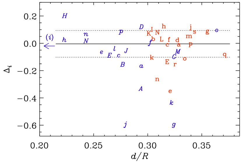
Figure 7.— The residual $\Delta_{i}$ versus $d/R$ for the K dwarfs (red symbols) listed in Table LABEL:Kstars, and the F and G dwarfs (blue symbols) listed in Table LABEL:Gstars. The solid horizontal line marks the average, and the dotted horizontal lines the standard deviation. As elsewhere, the red e and n symbols, as well as the blue $A$, $H$, $E$, $j$, and $g$ symbols are excluded from the fit. The blue $k$ symbol is, however, included.

It turns out that, within error bars, $\Delta_{i}$ does not vary systematically with $d/R$. Thus, if $\omega_{\rm cyc}/\Omega$ is indeed independent of $d/R$, we can expect that the correlation length of the dynamo is the same in stars with different values of $d/R$. This is remarkable, and suggests that changes in the depth of the convection zone are not important for the operation of stellar dynamos. However, the values of $\omega_{\rm cyc}/\Omega$ are different by a factor $\tilde{b}_{\rm I}/\tilde{b}_{\rm A}\approx 6$ on the two branches. This could be related to separate types of dynamos in a star, which are characterized by different correlation lengths. On the branch with a cycle 6 times longer, $(\omega_{\rm cyc}/\Omega)^{2}$ is 36 times smaller, and thus the correlation length is expected to be 36 times shorter. Shorter correlation lengths are normally associated with stellar surface layers, where the pressure scale height is smaller. This conclusion agrees with that of BV, who associated the active branch with a dynamo operating in the near-surface shear layer. This may well be compatible with the interpretation of See et al. (2016), who found that the magnetic topology on the active branch has a strong toroidal component. Strong toroidal fields are suggestive of a shallow origin, whereas deeply rooted dynamos are expected to exhibit mostly poloidal fields at the surface.

The idea of different dynamos was already proposed by Durney et al. (1981) to explain the Vaughan–Preston gap. Although Durney et al. (1981) argued in favor of a change of magnetic field topology, BV talked explicitly about the simultaneous operation of two dynamos. She imagined both of them being interface dynamos, but that the dynamo on the inactive branch would be affected by mixing in deeper layers, whereas that on the active branch would operate preferentially in the near-surface shear layers of rapidly rotating G dwarfs. Meanwhile, global convective dynamo simulations (Brown et al., 2010; Racine et al., 2011; Käpylä et al., 2012) have produced magnetic fields in the bulk of the convection zone. Some of the simulations have demonstrated the simultaneous occurrence of multiple dynamo periods within the same star (Käpylä et al., 2016; Beaudoin, 2016). In the simulations of Käpylä et al. (2013), I and A branches have been found that were separated by a factor of four in $\omega_{\rm cyc}/\Omega$. These simulations produced longer periods near the bottom of the convection zone. By contrast, earlier mean-field models of Covas et al. (2000, 2001) resulted in shorter periods, which would be in agreement with our interpretation. It would therefore be interesting to see whether any of these models can produce cycle diagnostics similar to those discussed in the present paper.

4.2. Dependence on metallicity

To see whether unusual metallicities can be responsible for some of the systematic departures between the observed and computed cycle periods, we plot the dependence of $\Delta_{i}$ on [Fe/H] in Figure 8. It turns out that the stars with the largest departures from $\Delta_{i}=0$ all have moderate values of [Fe/H]; see HD 78366 (blue $g$ symbol) and HD 114710 (blue $j$ symbol), for which $\Delta_{i}\approx-0.55\,{\rm dex}$ and HD 100180 (blue $H$ symbol), for which $\Delta_{i}\approx+0.25\,{\rm dex}$. Thus, we conclude that there is no systematic trend between $\Delta_{i}$ and [Fe/H]. Conversely, the star with the smallest metallicity (HD 103095, blue $i$ symbol) has ${\rm[Fe/H]}=-1.36$, but the cycle period of $7.3\,{\rm yr}$ agrees well with the computed one of $8.2\,{\rm yr}$.

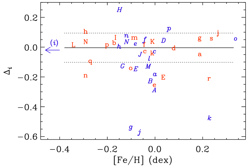
Figure 8.— The residual $\Delta_{i}$ versus [Fe/H]. Otherwise like Figure 7.

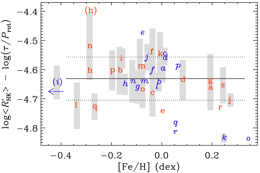
Figure 9.— Plot of the residual $\log\langle R^{\prime}_{\rm HK}\rangle-\log(\tau/P_{\rm rot})$ versus [Fe/H] for the K dwarfs of Table LABEL:Kstars in red roman symbols, together with the F and G dwarfs of Table LABEL:Gstars in blue italics symbols. The cycle amplitude is indicated by the vertical extent of the gray boxes. The solid horizontal line marks the average, and the dotted horizontal lines the standard deviation. The red h symbol marks the location of HD 81809 for $B-V=0.80$ whereas “(h)” indicates where the location would be if the value $B-V=0.64$ from Egeland (2017) were adopted.

Stars with higher (lower) metallicity have a larger (smaller) convection zone thickness, thereby mimicking properties of stars of later (earlier) spectral type that have larger (smaller) values of $\tau$. This could imply larger (smaller) values of $\langle R^{\prime}_{\rm HK}\rangle$, and hence smaller (larger) values of $\Delta_{i}$. One would then expect a negative slope in Figure 8. No reliable slope is found, although it is interesting to note that this would be in the right direction to explain the departure found for HD 128620 (blue $k$ symbol). This argument would assume that the approximately linear relation between $\langle R^{\prime}_{\rm HK}\rangle$ and $\tau/P_{\rm rot}$ remains valid and that the $c$ in Equation (5) does not itself depend on [Fe/H]. Figure 9 shows that this is indeed the case.

In this connection, we recall that, for HD 81809 (red h symbol), we assumed $B-V=0.80$, which might not be justified (Egeland, 2017). If we were to use $B-V=0.64$, the value of $\tau$ would be smaller, and therefore $c$ would be larger. This point is marked in Figure 9 with “(h),” which exceeds the average value of $c$ by more than $0.2\,{\rm dex}$. On the other hand, if HD 81809 is indeed a subgiant, as argued by Egeland (2017), then Equation (5) might not be valid without additional adjustments.

4.3. Dependence on age

Stellar activity decreases monotonically with age for dwarfs, so it is instructive to plot the residual $c$ from Equation (11) versus $\log\langle R^{\prime}_{\rm HK}\rangle$. Figure 10 shows that Equation (5) begins to fail for the smallest values of $\log\langle R^{\prime}_{\rm HK}\rangle<-5.0$. Stars with very low activity are “superrotating,” i.e., they rotate faster than expected based on their activity level. This is again a clear indication that these stars, notably 16 Cyg A and B (blue $q$ and $r$ symbols), $\alpha$ Cen A (blue $k$ symbol), and KIC 8006161 (blue $o$ symbol), have experienced reduced magnetic braking as a consequence of the large-scale cyclic dynamo having started to shut down (Kitchatinov & Nepomnyashchikh, 2017). For 16 Cyg A and B (blue $q$ and $r$ symbols in Figure 10), this has already happened.

As discussed by BV, the coexistence of long and short period cycles in some stars suggests that multiple stellar dynamos can operate simultaneously. As we have seen from Table LABEL:DoubleCycles, this is a possibility for all stars younger than about $2.3\,{\rm Gyr}$. This interpretation offers a fresh opportunity to consider the evolution of stellar cycles in the BST diagram as stars move from high levels of activity (right side of Figure 5) toward lower activity states (left side of Figure 5).

Evidently, long period cycles are dominant for stars on the active side of the Vaughan–Preston gap, whereas short period cycles dominate on the inactive side. This idea may help to explain some of the outliers discussed above. In particular, the short period cycle in HD 22049 (red e symbol), which is very young ($0.6\,{\rm Gyr}$), may be operating outside the optimal range of the underlying dynamo, so it falls below the pattern established by other cycles on the inactive branch. By contrast, HD 165341A (red n symbol) and HD 149661 (red k symbol) are older, and their short cycles agree reasonably well with the computed ones. HD 30495 (blue $e$ symbol) is also fairly young ($1.1\,{\rm Gyr}$), but its short cycle period agrees with stars on the inactive branch. Evolving toward the Vaughan–Preston gap, short period cycles begin to appear slightly above the inactive branch (blue $f$ and $p$ symbols). At comparable activity levels, we see coexisting long and short cycles for HD 78366 (blue $G/g$ symbols) and HD 114710 (blue $J/j$ symbols). The long cycles in these stars fall on the active branch, whereas the short cycles appear to be outliers. Just across the Vaughan–Preston gap, we find HD 190406 (blue $N/n$ symbols), which is the only star in the sample with long and short period cycles that both fall directly onto their respective branches. At an age of $2.1\,{\rm Gyr}$, it is no longer very young.

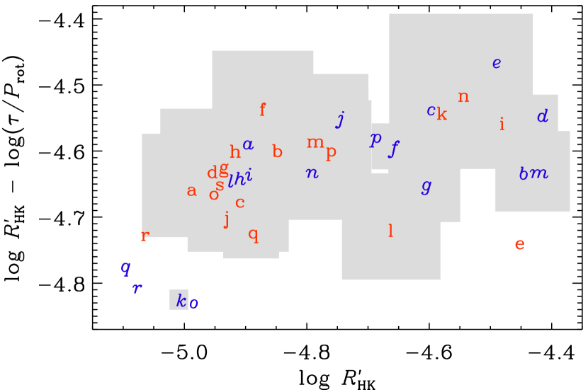
Figure 10.— Residual $\log\langle R^{\prime}_{\rm HK}\rangle-\log(\tau/P_{\rm rot})$ versus $\log\langle R^{\prime}_{\rm HK}\rangle$ for the K dwarfs in red roman characters, together with the F and G dwarfs in blue italics characters. The cycle amplitude is indicated by the vertical extent of the gray boxes, whereas the horizontal extent denotes the spread of $\log\langle R^{\prime}_{\rm HK}\rangle$ between cycle minimum and maximum. Note the systematic departures for small values of $\log\langle R^{\prime}_{\rm HK}\rangle$.

Moving to lower activity levels we find HD 100180 (blue $H/h$ symbols) at $2.3\,{\rm Gyr}$, which shows a short period cycle on the inactive branch and a long period cycle that falls above the active branch. This could signal the operation of the underlying dynamo beyond its optimal range, although the long period cycles might simply exceed the reach of current time domain surveys. Below a critical activity level, even the inactive branch may no longer sustain coherent stellar cycles. Based on the positions of two solar analogs in the BV diagram, Metcalfe et al. (2017) suggest that the short period cycle in HD 146233 (blue $l$ symbol, $4.1\,{\rm Gyr}$) may evolve away from the inactive branch toward the longer period cycle in HD 128620 (blue $k$ symbol, $5.4\,{\rm Gyr}$) before the cycle disappears entirely, as in the old solar analogs 16 Cyg A and B (Hall et al., 2007a; Metcalfe et al., 2015) at $7\,{\rm Gyr}$. This transition appears to coincide with the reduced magnetic braking suggested by van Saders et al. (2016), possibly due to a reconfiguration of the field toward smaller spatial scales as the global dynamo begins to shut down (Metcalfe et al., 2016). The Sun (blue $a$ symbol, $4.6\,{\rm Gyr}$) appears to be on the threshold of this transition, particularly during solar minimum. The absence of additional points at lower activity levels may simply reflect the disappearance of cycles below this threshold (Metcalfe & van Saders, 2017). Future observations of inactive Kepler stars will help to clarify this picture.

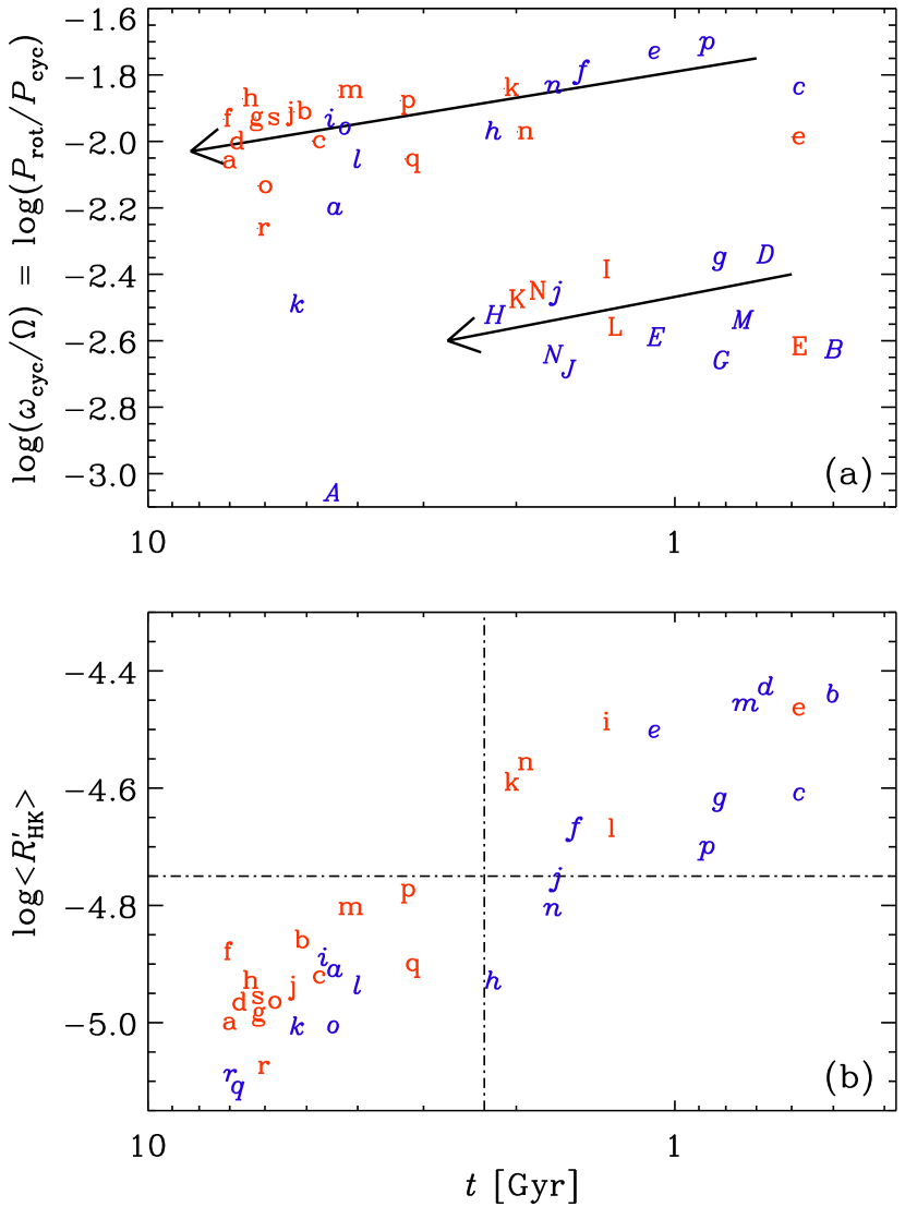
Figure 11.— (a) Frequency ratio versus age. Note that age increases to the left, to facilitate comparison with the BST diagram. The arrows indicate tentative evolutionary tracks. (b) $\langle R^{\prime}_{\rm HK}\rangle$ versus age.

BST assumed that $\langle R^{\prime}_{\rm HK}\rangle$ was a reasonable proxy of age. Gyrochronology and asteroseismology allow us now to express the frequency ratio directly in terms of age; see Section 2.3. A BST plot with age on the abscissa is shown in Figure 11(a). Compared to the BST plot in Figure 5, the scatter is larger. However, both plots agree, in that the long and short cycle branches overlap in the ranges

$$-4.85\leq\langle R^{\prime}_{\rm HK}\rangle\leq-4.45,\quad 0.6\leq t/{\rm Gyr}\leq 2.3,$$ (12)

where both branches are populated. This is different from the original BST plot, where the overlap is almost absent.

In Figure 11(b), we show $\langle R^{\prime}_{\rm HK}\rangle$ versus age. It shows that all stars older than $2.3\,{\rm Gyr}$ have an $\langle R^{\prime}_{\rm HK}\rangle$ value below the Vaughan–Preston gap. Most of the younger stars are above the Vaughan–Preston gap, except HD 100180 (blue $h$ symbol), HD 114710 (blue $j$ symbol), and HD 190406 (blue $n$ symbol), which are below the gap. These exceptions are all G dwarfs with two cycle periods. This shows that all stars with long cycle periods are younger than $2.3\,{\rm Gyr}$ – even the rather inactive stars HD 190406 (blue $n$ symbol) and HD 100180 (blue $h$ symbol) in the lower right quadrant of Figure 11b.

The reverse is not true: many stars with short cycle periods can still be young and may only have a short cycle, namely HD 17051 (blue $c$ symbol with $P_{\rm cyc}=1.6\,{\rm yr}$). HD 76151 (blue $f$ symbol with $P_{\rm cyc}=2.5\,{\rm yr}$), and KIC 10644253 (blue $p$ symbol with $P_{\rm cyc}=1.5\,{\rm yr}$). However, it would be important to keep looking for longer secondary cycle periods, which may already have been found in the case of HD 76151 (Egeland, 2017).

Pace et al. (2009) have suggested that the evolution across the Vaughan–Preston gap may be rather abrupt. Our Figure 11(b) could be compatible with this idea, especially for the F dwarfs, where we find several stars in a narrow interval around $1.7\,{\rm Gyr}$ outlining a jump in $\langle R^{\prime}_{\rm HK}\rangle$. For the K dwarfs, this may also happen, but it would be somewhat later—between $2$ and $3\,{\rm Gyr}$, although in our sample has no K dwarfs in that age range.

5. Conclusions

The present work supports the idea that longer and shorter stellar cycles tend to fall on one of two universal branches in the BST diagram. In the corresponding BV diagram, these lines are not universal, but correspond to a family of lines for different values of the turnover time. For K dwarfs, the values of $\tau$ lie within a relatively narrow range between $17$ and $23\,{\rm d}$, so the statistical quality between the BST and BV diagrams is similar. For F and G stars, on the other hand, the scatter is significantly larger in both the BST and BV diagrams.

It was already known that the BST diagram can be cast into an evolutionary diagram. However, unlike the previous interpretation whereby young stars would evolve along the active or long cycle period branch, we now see that all stars younger than $2.3\,{\rm Gyr}$ are capable of exhibiting longer and shorter cycle periods. This implies that the solar Gleissberg cycle would not be a secondary cycle in the same sense, because the Sun is older than $2.3\,{\rm Gyr}$.

Our work has allowed us to compute secondary cycle periods that could be longer or shorter than the observed ones. It will be interesting to see whether this is borne out by future observations. For some stars, the possibility of as yet undetected shorter cycle periods in the $1$–$2\,{\rm yr}$ range is now a possibility, notably for the G dwarfs HD 1835, HD 20630, and HD 152391. Less clear is the situation for the K dwarfs HD 115404 and HD 156026, for which shorter cycle periods in the $3$–$4\,{\rm yr}$ range are possible. On the other hand, for the G dwarfs HD 76151 and KIC 10644253, for which shorter cycle periods have been detected, longer periods in the $12$–$16\,{\rm yr}$ range are possible, and may have been already found in the case of HD 76151 (Egeland, 2017). Similarly, for $\iota$ Hor (HD 17051), the star with a short cycle of $1.6\,{\rm Gyr}$, a longer $\sim 5\,{\rm yr}$ cycle may have already emerged (Flores et al., 2017). If this possibility gets confirmed, it will be interesting to see how the measured period would compare with the computed cycle of $8.5\,{\rm yr}$. Such a time frame would be more manageable than those associated with the secondary Gleissberg-type cycles of solar-like stars. On the other hand, our work now suggests that the Gleissberg cycle of the Sun is distinct from the longer secondary cycles discussed here for our sample of ten stars.

We have found no systematic dependence of the period ratio or the activity level on metallicity or $d/R$. This suggests that these aspects of the dynamo are not strongly affected by the depth of the star’s convection zone. This would be more suggestive of distributed dynamos, although it would be premature to make strong claims whereas the solar dynamo is not yet well understood. For the most inactive stars, cyclic dynamo activity has ceased and the chromospheric activity level has dropped below the value that is expected based on the star’s rotation rate.

References

- Ayres (2014) Ayres, T. R. 2014, AJ, 147, 59
- Ayres (2015) Ayres, T. R. 2015, AJ, 149, 58
- Baliunas & Vaughan (1985) Baliunas, S. L., & Vaughan, A. H. 1985, ARA&A, 23, 379
- Baliunas et al. (1995) Baliunas, S. L., Donahue, R. A., Soon, W. H., Horne, J. H., Frazer, J., Woodard-Eklund, L., Bradford, M., Rao, L. M., Wilson, O. C., Zhang, Q., Bennett, W., Briggs, J., Carroll, S. M., Duncan, D. K., Figueroa, D., Lanning, H. H., Misch, T., Mueller, J., Noyes, R. W., Poppe, D., Porter, A. C., Robinson, C. R., Russell, J., Shelton, J. C., Soyumer, T., Vaughan, A. H., & Whitney, J. H. 1995, ApJ, 438, 269
- Baliunas et al. (1996) Baliunas, S. L., Nesme-Ribes, E., Sokoloff, D., & Soon, W. H. 1996, ApJ, 460, 848
- Barekat et al. (2014) Barekat, A., Schou, J., & Gizon, L. 2014, A&AL, 570, L12
- Bazot et al. (2007) Bazot, M., Bouchy, F., Kjeldsen, H., Charpinet, S., Laymand, M., & Vauclair, S. 2007, A&A, 470, 295
- Bazot et al. (2012) Bazot, M., Bourguignon, S., & Christensen-Dalsgaard, J. 2012, MNRAS, 427, 1847
- Beaudoin (2016) Beaudoin, P., Simard, C., Cossette, J.-F., & Charbonneau, P. 2016, ApJ, 826, 138
- Böhm-Vitense (2007) Böhm-Vitense, E. 2007, ApJ, 657, 486 (BV)
- Boro Saikia et al. (2016) Boro Saikia, S., Jeffers, S. V., Morin, J., Petit, P., Folsom, C. P., Marsden, S. C., Donati, J.-F., Cameron, R., Hall, J. C., Perdelwitz, V., Reiners, A., & Vidotto, A. A. 2016, A&A, 594, A29
- Brandenburg (2005) Brandenburg, A. 2005, ApJ, 625, 539
- Brandenburg & Schmitt (1998) Brandenburg, A., & Schmitt, D. 1998, A&AL, 338, L55
- Brandenburg et al. (1998) Brandenburg, A., Saar, S. H., & Turpin, C. R. 1998, ApJL, 498, L51 (BST)
- Brown et al. (2010) Brown, B. P., Browning, M. K., Brun, A. S., Miesch, M. S., & Toomre, J. 2010, ApJ, 711, 424
- Buchhave & Latham (2015) Buchhave, L. A., & Latham, D. W. 2015, ApJ, 808, 187
- Chatterjee et al. (2011) Chatterjee, P., Mitra, D., Rheinhardt, M., & Brandenburg, A. 2011, A&A, 534, A46
- Choudhuri et al. (1995) Choudhuri, A. R., Schüssler, M., & Dikpati, M. 1995, A&AL, 303, L29
- Covas et al. (2000) Covas, E., Tavakol, R., & Moss, D. 2000, A&AL, 363, L13
- Covas et al. (2001) Covas, E., Tavakol, R., Vorontsov, S., & Moss, D. 2001, A&A, 375, 260
- Creevey et al. (2017) Creevey, O. L., Metcalfe, T. S., Schultheis, M., Salabert, D., Bazot, M., Thévenin, F., Mathur, S., Xu, H., & García, R. A. 2017, A&A, 601, A67
- Dikpati & Charbonneau (1999) Dikpati, M., & Charbonneau, P. 1999, ApJ, 518, 508
- Donahue et al. (1996) Donahue, R. A., Saar, S. H., & Baliunas, S. L. 1996, ApJ, 466, 384
- Durney et al. (1981) Durney, B. R., Mihalas, D., & Robinson, R. D. 1981, PASP, 93, 537
- Eberhard & Schwarzschild (1913) Eberhard, G., & Schwarzschild, K. 1913, ApJ, 38, 292
-
Egeland (2017)
Egeland, R., 2017, PhD thesis, Montana State University,
http://www.physics.montana.edu/people/students/regeland - Egeland et al. (2015) Egeland, R., Metcalfe, T. S., Hall, J. C., & Henry, G. W. 2015, ApJ, 812, 12
- Ferreira Lopes et al. (2015) Ferreira Lopes, C. E., Leão, I. C., de Freitas, D. B., Canto Martins, B. L., Catelan, M., & De Medeiros, J. R. 2015, A&A, 583, A134
- Flores et al. (2017) Flores, M. G., Buccino, A. P., Saffe, C. E., & Mauas, P. J. D. 2017, MNRAS, 464, 4299
- Fuhrmann (2008) Fuhrmann, K. 2008, MNRAS, 384, 173
- García et al. (2010) García, R. A., Mathur, S., Salabert, D., Ballot, J., Régulo, C., Metcalfe, T. S., & Baglin, A. 2010, Science, 329, 1032
- García et al. (2014) García, R. A., Ceillier, T., Salabert, D., Mathur, S., van Saders, J. L., Pinsonneault, M., Ballot, J., Beck, P. G., Bloemen, S., Campante, T. L., Davies, G. R., do Nascimento, J.-D., Jr., Mathis, S., Metcalfe, T. S., Nielsen, M. B., Suárez, J. C., Chaplin, W. J., Jiménez, A., & Karoff, C. 2014, A&A, 572, A34
- Gray et al. (2006) Gray, R. O., Corbally, C. J., Garrison, R. F., McFadden, M. T., Bubar, E. J., McGahee, C. E., O’Donoghue, A. A., & Knox, E. R. 2006, ApJ, 132, 161
- Hall et al. (2007a) Hall, J. C., Lockwood, G. W., & Skiff, B. A. 2007a, AJ, 133, 862
- Hall et al. (2007b) Hall, J. C., Henry, G. W., & Lockwood, G. W. 2007b, AJ, 133, 2206
- Hallam et al. (1991) Hallam, K. L., Altner, B., & Endal, A. S. 1991, ApJ, 372, 610
- Jouve et al. (2010) Jouve, L., Brown, B. P., & Brun, A. S. 2010, A&A, 509, A32
- Käpylä et al. (2012) Käpylä, P. J., Mantere, M. J., & Brandenburg, A. 2012, ApJL, 755, L22
- Käpylä et al. (2013) Käpylä, P. J., Mantere, M. J., Cole, E., Warnecke, J., & Brandenburg, A. 2013, ApJ, 778, 41
- Käpylä et al. (2016) Käpylä, M. J., Käpylä, P. J., Olspert, N., Brandenburg, A., Warnecke, J., Karak, B. B., & Pelt, J. 2016, A&A, 589, A56
- Karak et al. (2014) Karak, B. B., Kitchatinov, L. L., & Choudhuri, A. R. 2014, ApJ, 791, 59
- Kervella et al. (2008) Kervella, P., Mérand, A., Pichon, B., Thévenin, F., Heiter, U., Bigot, L., ten Brummelaar, T. A., McAlister, H. A., Ridgway, S. T., Turner, N., Sturmann, J., Sturmann, L., Goldfinger, P. J., & Farrington, C. 2008, A&A, 488, 667
- Kiefer et al. (2017) Kiefer, R., Schad, A., Davies, G., & Roth, M. 2017, A&A, 598, A77
- Kitchatinov & Nepomnyashchikh (2017) Kitchatinov, L., & Nepomnyashchikh, A. 2017, MNRAS, 470, 3124
- Kleeorin et al. (1983) Kleeorin, N. I., Ruzmaikin, A. A., & Sokoloff, D. D. 1983, Ap&SS, 95, 131
- Kochukhov et al. (2011) Kochukhov, O., Makaganiuk, V., Piskunov, N., Snik, F., Jeffers, S. V., Johns-Krull, C. M., Keller, C. U., Rodenhuis, M., & Valenti, J. A. 2011, ApJL, 732, L19
- Lehtinen et al. (2016) Lehtinen, J., Jetsu, L., Hackman, T., Kajatkari, P., & Henry, G. W. 2016, A&A, 588, A38
- Li et al. (2012) Li, T. D., Bi, S. L., Liu, K., Tian, Z. J., & Shuai, G. Z. 2012, A&A, 546, A83
- Mamajek & Hillenbrand (2008) Mamajek, E. E., & Hillenbrand, L. A. 2008, ApJ, 687, 1264
- Marsden et al. (2014) Marsden, S. C., Petit, P., Jeffers, S. V., Morin, J., Fares, R., Reiners, A., do Nascimento, J.-D., Auriére, M., Bouvier, J., Carter, B. D., Catala, C., Dintrans, B., Donati, J.-F., Gastine, T., Jardine, M., Konstantinova-Antova, R., Lanoux, J., Ligniéres, F., Morgenthaler, A., Ramírez-Vèlez, J. C., Th’eado, S., Van Grootel, V., & BCool Collaboration 2014, MNRAS, 444, 3517
- Mathur et al. (2014) Mathur, S., García, R. A., Ballot, J., Ceillier, T., Salabert, D., Metcalfe, T. S., Régulo, C., Jiménez, A., & Bloemen, S. 2014, A&A, 562, A124
- Metcalfe et al. (2010) Metcalfe, T. S., Basu, S., Henry, T. J., Soderblom, D. R., Judge, P. G., Knölker, M., Mathur, S., & Rempel, M. 2010, ApJL, 723, L213
- Metcalfe et al. (2013) Metcalfe, T. S., Buccino, A. P., Brown, B. P., Mathur, S., Soderblom, D. R., Henry, T. J., Mauas, P. J. D., Petrucci, R., Hall, J. C., Basu, S. 2013, ApJL, 763, L26
- Metcalfe et al. (2015) Metcalfe, T. S., Creevey, O. L., & Davies, G. R. 2015, ApJL, 811, L37
- Metcalfe et al. (2016) Metcalfe, T. S., Egeland, R., & van Saders, J. 2016, ApJ, 826, L2
- Metcalfe et al. (2017) Metcalfe, T., Creevey, O., & van Saders, J. 2017, Proceedings of the 22nd Los Alamos Stellar Pulsation Conference, submitted (arXiv:1701.08746)
- Metcalfe & van Saders (2017) Metcalfe, T. S., & van Saders, J. 2017, Sol. Phys., in press, arXiv:1705.09668
- Mittag et al. (2016) Mittag, M., Schröder, K.-P., Hempelmann, A., González-Pérez, J. N., & Schmitt, J. H. M. M. 2016, A&A, 591, A89
- Montet et al. (2017) Montet, B. T., Tovar, G., & Foreman-Mackey, D. 2017, ApJ, submitted, arXiv:1705.07928
- Morgenthaler et al. (2011) Morgenthaler, A., Petit, P., Morin, J., Aurière, M., Dintrans, B., Konstantinova-Antova, R., & Marsden, S. 2011, Astron. Nachr., 332, 866
- Nordström et al. (2004) Nordström, B., Mayor, M., Andersen, J., Holmberg, J., Pont, F., Jørgensen, B. R., Olsen, E. H., Udry, S., & Mowlavi, N. 2004, A&A, 418, 989
- Noyes (1983) Noyes, R. W. 1983, in Solar and stellar magnetic fields: Origins and coronal effects, Proceedings of the Symposium, Zurich, Switzerland, August 2-6, 1982, ed. J. O. Stenflo (Dordrecht, D. Reidel Publishing Co.), 133
- Noyes et al. (1984a) Noyes, R. W., Hartmann, L., Baliunas, S. L., Duncan, D. K., & Vaughan, A. H. 1984a, ApJ, 279, 763
- Noyes et al. (1984b) Noyes, R. W., Weiss, N. O., & Vaughan, A. H. 1984b, ApJ, 287, 769
- Olah et al. (2016) Oláh, K., Kővári, Z., Petrovay, K., Soon, W., Baliunas, S., Kolláth, Z., Vida, K. 2016, A&A, 590, A133
- Pace et al. (2009) Pace, G., Melendez, J., Pasquini, L., Carraro, G., Danziger, J., François, P., Matteucci, F., & Santos, N. C. 2009, A&A, 499, L9
- Parker (1955) Parker, E. N. 1955, ApJ, 122, 293
- Parker (1975) Parker, E. N. 1975, ApJ, 198, 205
- Pipin & Kosovichev (2011) Pipin, V. V., & Kosovichev, A. G. 2011, ApJ, 727, L45
- Racine et al. (2011) Racine, É., Charbonneau, P., Ghizaru, M., Bouchat, A., & Smolarkiewicz, P. K. 2011, ApJ, 735, 46
- Ramírez et al. (2013) Ramírez, I., Allende Prieto, C., & Lambert, D. L. 2013, ApJ, 764, 78
- Reinhold et al. (2017) Reinhold, T., Cameron, R. H., & Gizon, L. 2017, A&A, 603, A52
- Robinson & Durney (1982) Robinson, R. D., & Durney, B. R. 1982, A&A, 108, 322
- Saar & Baliunas (1992) Saar, S. H., & Baliunas, S. L. 1992, in The Solar Cycle, Proceedings of the NSO/Sac Peak 12th Summer Workshop, ed. K. L. Harvey (ASP Conf. Series, Vol. 27), 150
- Saar & Brandenburg (1999) Saar, S. H., & Brandenburg, A. 1999, ApJ, 524, 295
- Saar & Brandenburg (2002) Saar, S. H., & Brandenburg, A. 2002, Astron. Nachr., 323, 357
- Saar & Linsky (1985) Saar, S. H., & Linsky, J. L. 1985, ApJ, 299, L47
- Salabert et al. (2016a) Salabert, D., Régulo, C., García, R. A., Beck, P. G., Ballot, J., Creevey, O. L., Pérez Hernández, F., do Nascimento, J.-D., Jr., Corsaro, E., Egeland, R., Mathur, S., Metcalfe, T. S., Bigot, L., Ceillier, T., & Pallé, P. L. 2016a, A&A, 589, A118
- Salabert et al. (2016b) Salabert, D., García, R. A., Beck, P. G., Egeland, R., Pallé, P. L., Mathur, S., Metcalfe, T. S., do Nascimento, J.-D., Jr., Ceillier, T., Andersen, M. F., & Triviño Hage, A. 2016b, A&A, 596, A31
- Santos et al. (2010) Santos, N. C., Gomes da Silva, J., Lovis, C., & Melo, C. 2010, A&A, 511, A54
- Schou et al. (1998) Schou, J., Antia, H. M., Basu, S., Bogart, R. S., Bush, R. I., Chitre, S. M., Christensen-Dalsgaard, J., di Mauro, M. P., Dziembowski, W. A., Eff-Darwich, A., Gough, D. O., Haber, D. A., Hoeksema, J. T., Howe, R., Korzennik, S. G., Kosovichev, A. G., Larsen, R. M., Pijpers, F. P., Scherrer, P. H., Sekii, T., Tarbell, T. D., Title, A. M., Thompson, M. J., & Toomre, J. 1998, ApJ, 505, 390
- Schrijver et al. (1989) Schrijver, C. J., Cote, J, Zwaan, C., & Saar, S. H. 1989, ApJ, 337, 964
- See et al. (2016) See, V., Jardine, M., Vidotto, A. A., Donati, J.-F., Boro Saikia, S., Bouvier, J., Fares, R., Folsom, C. P., Gregory, S. G., Hussain, G., Jeffers, S. V., Marsden, S. C., Morin, J., Moutou, C., do Nascimento, J. D., Petit, P., & Waite, I. A. 2016, MNRAS, 462, 4442
- Soon et al. (1993) Soon, W. H., Baliunas, S. L., & Zhang, Q. 1993, ApJL, 414, L33
- Steenbeck & Krause (1969) Steenbeck, M., & Krause, F. 1969, Astron. Nachr., 291, 49
- Stix (1976) Stix, M. 1976, in Basic Mechanisms of solar activity, ed. V. Bumba & J. Kleczek (IAU Symp. 71), 367
- Tuominen et al. (1988) Tuominen, I., Rüdiger, G., & Brandenburg, A. 1988, in Activity in Cool Star Envelopes, ed. O. Havnes, B. R. Pettersen, J. H. M. M. Schmitt, J. E. Solheim (Kluwer Acad. Publ.), 13
- van Saders & Pinsonneault (2012) van Saders, J. L., & Pinsonneault, M. H. 2012, ApJ, 746, 16
- van Saders et al. (2016) van Saders, J. L., Ceillier, T., Metcalfe, T. S., Silva Aguirre, V., Pinsonneault, M. H., García, R. A., Mathur, S., & Davies, G. R. 2016, Nature, 529, 181
- Vauclair et al. (2008) Vauclair, S., Laymand, M., Bouchy, F., Vauclair, G., Hui Bon Hoa, A., Charpinet, S., & Bazot, M. 2008, A&AL, 482, L5
- Vaughan & Preston (1980) Vaughan, A. H., & Preston, G. W. 1980, PASP, 92, 385
- Wilson (1963) Wilson, O. C. 1963, ApJ, 138, 832
- Wilson (1968) Wilson, O. C. 1968, ApJ, 153, 221
- Wilson (1978) Wilson, O. C. 1978, ApJ, 266, 379