Unification of Dark Matter - Dark Energy in Generalized Galileon Theories

Abstract

We present a unified description of the dark matter and the dark energy sectors, in the framework of shift-symmetric generalized Galileon theories. Considering a particular combination of terms in the Horndeski Lagrangian in which we have not introduced a cosmological constant or a matter sector, we obtain an effective unified cosmic fluid whose equation of state $w_{U}$ is zero during the whole matter era, namely from redshifts $z\sim 3000$ up to $z\sim 2-3$. Then at smaller redshifts it starts decreasing, passing the bound $w_{U}=-1/3$, which marks the onset of acceleration, at around $z\sim 0.5$. At present times it acquires the value $w_{U}=-0.7$. Finally, it tends toward a de-Sitter phase in the far future. This behaviour is in excellent agreement with observations. Additionally, confrontation with Supernovae type Ia data leads to a very efficient fit. Examining the model at the perturbative level, we show that it is free from pathologies such as ghosts and Laplacian instabilities, at both scalar and tensor sectors, at all times.

I Introduction

Recent observations revealed that the Universe has entered a period of accelerated expansion acceleration ; ries . Within the framework of General Relativity (GR), the accelerated expansion can be driven by a new energy density component with negative pressure, termed Dark Energy (DE) Copeland:2006wr , the nature of which is unknown, although the cosmological constant might be the most reasonable candidate. On the other hand, the missing mass in individual galaxies, as well as their large scale structure distributions in the whole universe, is attributed to a new form of matter, termed Cold Dark Matter (CDM), which is assumed to have negligible pressure. The consideration of these two dark components, along with the usual standard model of particles, constitutes the concordance model of cosmology, namely the $\Lambda$CDM paradigm.

Extensions of $\Lambda$CDM concordance model can arise either modifying the gravitational sector, departing from GR, or maintaining GR but altering the nature of DE and/or DM. In the first approach, namely of modified gravity (for a review see Joyce:2014kja ), one introduces extra geometric terms in the action, or extra scalar fields which are non-minimally coupled to gravity. In the second approach, one considers that the DE sector is dynamic, evolving with time, with a possible additional interaction with the DM sector. Such interacting dark sectors (for a recent review on the dark matter - dark energy interaction see Wang:2016lxa ) will affect the overall evolution of the Universe and its expansion history, the growth of dark matter and baryon density perturbations, the pattern of temperature anisotropies of the Cosmic Microwave Background (CMB) radiation and the evolution of the gravitational potential at late times. This approach may also alleviate the cosmic coincidence problem, i.e. the question of why the DE and DM energy densities are currently of the same order, although they follow different evolution laws. These observables are directly linked to the underlying theory of gravity and, consequently, the interaction could be constrained by the observational data Bolotin:2013jpa .

In a parallel development there has been a large amount of effort in order to understand and describe the thermal history of the universe in a unified way. Amongst others one could consider that the energy density might be regulated by the change in the equation of state of a background exotic fluid, the Chaplygin gas. The main motivation of considering the Chaplygin gas Bento:2002ps was to introduce an equation of state parameter which can mimic a pressureless fluid at the early stages of the universe evolution, and a quintessence-like sector at late times, tending asymptotically to a cosmological constant. The generalized Chaplygin gas is efficient in describing the universe evolution at the background level in agreement with observations Bento:2002yx ; Bento:2005un , but it may be plagued by the presence of instabilities as well as oscillations which are not observed in the matter power spectrum Sandvik:2002jz . Nevertheless, one can introduce various mechanisms in order to bypass such problems, for instance allowing for small entropy perturbations Farooq:2010xm ; Gorini:2007ta or for the addition of baryons which can improve the behaviour of the matter power spectrum Debnath:2004cd ; BouhmadiLopez:2004mp ; Setare:2007mp .

Recently there are many studies of scalar tensor theories Fujii:2003pa and one of them is the Gravity theory resulting from the Horndeski Lagrangian Horndeski:1974wa . Horndeski theories are technically manageable, since they lead to second-order field equations, and they prove consistent without ghost instabilities Ostrogradsky:1850fid . Moreover, a subclass of these scalar tensor theories of modified gravity shares a classical Galilean symmetry which has been discovered independently Nicolis:2008in ; Deffayet:2009wt ; Deffayet:2009mn ; Deffayet:2011gz . When one generalizes Galileon theory abandoning shift symmetry, one reobtains Horndeski theory. In Horndeski theory the derivative self-couplings of the scalar field screen the deviations from GR at high gradient regions (small scales or high densities) through the Vainshtein mechanism Vainshtein:1972sx , thus satisfying solar system and early universe constraints Chow:2009fm ; DeFelice:2011th ; Babichev:2011kq ; Saridakis:2016ahq .

In this work we present a unified description of the dark matter and dark energy sectors in the framework of shift-symmetric generalized Galileon theory, which is different than the standard approach where the Galileon field plays solely the role of dark energy Chow:2009fm ; DeFelice:2011th ; Babichev:2011kq ; deRham:2011by ; Heisenberg:2014kea ; Saridakis:2016ahq , or the approach where it plays solely the role of dark matter Rinaldi:2016oqp . In particular, considering a subclass of Horndeski theory, without considering an explicit matter sector and an explicit cosmological constant, we show that the scalar field gives rise to an effective cosmic fluid with equation of state parameter that behaves as pressureless matter at early times, and as dark energy at late times. Additionally, by suitably choosing the model parameter regions, and without fine tuning, one can obtain the correct redshift behaviour and values of observables, in agreement with the observational data. Finally, examining the model at the perturbative level we show that, on top of the background unified solutions, it is free from pathologies such as ghosts and Laplacian instabilities at all times.

The manuscript is organized as follows. In Section II we briefly review the generalized Galileon cosmology. In Section III we present the general features of the dark matter - dark energy unification in the framework of shift-symmetric generalized Galileon theories, and in Section IV we construct a specific model, examining its cosmological application in detail. Finally, Section V is devoted to the summary of our results.

II Generalized Galileon cosmology

In this section we briefly review generalized Galileon theory, applying it to a cosmological framework and deriving the background equations as well as the conditions for the absence of instabilities DeFelice:2010nf ; DeFelice:2011bh . As it is known, in order to avoid the Ostrogradsky instability Ostrogradsky:1850fid it is required to keep the equations of motion at second order in derivatives, and thus the most general four-dimensional scalar tensor theories having second order field equations are described by the action

$$S=\int d^{4}x\sqrt{-g}\,{\cal L}\,,$$ (1)

where $g$ is the determinant of the metric $g_{\mu\nu}$, and where the Lagrangian reads Horndeski:1974wa

$${\cal L}=\sum_{i=2}^{5}{\cal L}_{i}\,,$$ (2)

with

$${\cal L}_{2}=K(\phi,X)~{},$$ (3)

$${\cal L}_{3}=-G_{3}(\phi,X)\Box\phi~{},$$ (4)

$${\cal L}_{4}=G_{4}(\phi,X)\,R+G_{4,X}\,[(\Box\phi)^{2}-(\nabla_{\mu}\nabla_{\nu}\phi)\,(\nabla^{\mu}\nabla^{\nu}\phi)]\,,$$ (5)

$${\cal L}_{5}=G_{5}(\phi,X)\,G_{\mu\nu}\,(\nabla^{\mu}\nabla^{\nu}\phi)\,$$

$$\ \ \ \ \ \ \ -\frac{1}{6}\,G_{5,X}\,[(\Box\phi)^{3}-3(\Box\phi)\,(\nabla_{\mu}\nabla_{\nu}\phi)\,(\nabla^{\mu}\nabla^{\nu}\phi)+2(\nabla^{\mu}\nabla_{\alpha}\phi)\,(\nabla^{\alpha}\nabla_{\beta}\phi)\,(\nabla^{\beta}\nabla_{\mu}\phi)]\,,$$ (6)

where for simplicity we have set the gravitational constant to $\kappa\equiv 8\pi G=1$. The functions $K$ and $G_{i}$ ($i=3,4,5$) depend on the scalar field $\phi$ and its kinetic energy $X=-\partial^{\mu}\phi\partial_{\mu}\phi/2$, while $R$ is the Ricci scalar, and $G_{\mu\nu}$ is the Einstein tensor. $G_{i,X}$ and $G_{i,\phi}$ ($i=3,4,5$) respectively correspond to the partial derivatives of $G_{i}$ with respect to $X$ and $\phi$, namely $G_{i,X}\equiv\partial G_{i}/\partial X$ and $G_{i,\phi}\equiv\partial G_{i}/\partial\phi$.

The action (1) was first found by Horndeski in Horndeski:1974wa , but it was independently rederived in the framework of Galileon theory. We mention here that in the original version of Galileon theory, shift symmetry plays a crucial role, and hence the two theories do not coincide. Nevertheless, extending Galileon theory to the so-called generalised Galileon theory, i.e abandoning the shift symmetry, leads to a complete identification with the Horndeski construction.

Let us now apply the above theory to a cosmological framework. We impose a flat Friedmann-Robertson-Walker (FRW) background metric of the form

$$ds^{2}=-N^{2}(t)dt^{2}+a^{2}(t)\delta_{ij}dx^{i}dx^{j},$$ (7)

where $t$ is the cosmic time, $x^{i}$ are the comoving spatial coordinates, $N(t)$ is the lapse function, and $a(t)$ is the scale factor. In FRW geometry, $\phi$ becomes a function of $t$ only, and hence $X(t)=\dot{\phi}^{2}(t)/2$.

We stress that in standard Galileon cosmology, apart from the above scalar tensor action (1) one needs to take into account the matter content of the universe, described by the Lagrangian ${\cal{L}}_{m}$, corresponding to a perfect fluid with energy density $\rho_{m}$ and pressure $p_{m}$. However, as we mentioned in the Introduction, in the present work we will not consider an explicit dark matter sector.

Varying the action (1) with respect to $N(t)$ and $a(t)$ respectively, and setting $N=1$, we obtain

$$2XK_{,X}-K+6X\dot{\phi}HG_{3,X}-2XG_{3,\phi}-6H^{2}G_{4}+24H^{2}X(G_{4,X}+XG_{4,XX})$$

$$-12HX\dot{\phi}\,G_{4,\phi X}-6H\dot{\phi}\,G_{4,\phi}+2H^{3}X\dot{\phi}\left(5G_{5,X}+2XG_{5,XX}\right)$$

$$-6H^{2}X\left(3G_{5,\phi}+2XG_{5,\phi X}\right)=0\,,$$ (8)

$$K-2X(G_{3,\phi}+\ddot{\phi}\,G_{3,X})+2(3H^{2}+2\dot{H})G_{4}-12H^{2}XG_{4,X}-4H\dot{X}G_{4,X}-8\dot{H}XG_{4,X}$$

$$-8HX\dot{X}G_{4,XX}+2(\ddot{\phi}+2H\dot{\phi})G_{4,\phi}+4XG_{4,\phi\phi}+4X(\ddot{\phi}-2H\dot{\phi})G_{4,\phi X}$$

$$-2X(2H^{3}\dot{\phi}+2H\dot{H}\dot{\phi}+3H^{2}\ddot{\phi})G_{5,X}-4H^{2}X^{2}\ddot{\phi}\,G_{5,XX}+4HX(\dot{X}-HX)G_{5,\phi X}$$

$$+2[2(\dot{H}X+H\dot{X})+3H^{2}X]G_{5,\phi}+4HX\dot{\phi}\,G_{5,\phi\phi}=0\,,$$ (9)

where dots denote derivatives with respect to $t$, and we also defined the Hubble parameter $H\equiv\dot{a}/a$. Variation of (1) with respect to $\phi(t)$ provides its evolution equation

$$\frac{1}{a^{3}}\frac{d}{dt}\left(a^{3}J\right)=P_{\phi}\,,$$ (10)

with

$$J \equiv \dot{\phi}K_{,X}+6HXG_{3,X}-2\dot{\phi}\,G_{3,\phi}+6H^{2}\dot{\phi}(G_{4,X}+2XG_{4,XX})-12HXG_{4,\phi X}$$ (11)

$$+2H^{3}X(3G_{5,X}+2XG_{5,XX})-6H^{2}\dot{\phi}(G_{5,\phi}+XG_{5,\phi X})\,,$$

$$P_{\phi} \equiv K_{,\phi}-2X\left(G_{3,\phi\phi}+\ddot{\phi}\,G_{3,\phi X}\right)+6(2H^{2}+\dot{H})G_{4,\phi}+6H(\dot{X}+2HX)G_{4,\phi X}$$ (12)

$$-6H^{2}XG_{5,\phi\phi}+2H^{3}X\dot{\phi}\,G_{5,\phi X}\,.$$

We close this section by mentioning that in order for the above scenario to be free of ghosts and Laplacian instabilities, and thus cosmologically viable, two conditions related to scalar perturbations must be satisfied DeFelice:2010pv ; DeFelice:2011bh ; Appleby:2011aa . In particular, for the scalar perturbations these read as DeFelice:2011bh

$$c_{S}^{2}\equiv\frac{3(2w_{1}^{2}w_{2}H-w_{2}^{2}w_{4}+4w_{1}w_{2}\dot{w}_{1}-2w_{1}^{2}\dot{w}_{2})}{w_{1}(4w_{1}w_{3}+9w_{2}^{2})}\geq 0~{},$$ (13)

for the avoidance of Laplacian instabilities associated with the scalar field propagation speed, and

$$Q_{S}\equiv\frac{w_{1}(4w_{1}w_{3}+9w_{2}^{2})}{3w_{2}^{2}}>0\,,$$ (14)

for the absence of ghosts, where

$$w_{1}\equiv 2\,(G_{{4}}-2\,XG_{{4,X}})-2X\,(G_{{5,X}}{\dot{\phi}}H-G_{{5,\phi}})\,,$$ (15)

$$w_{2}\equiv-2\,G_{{3,X}}X\dot{\phi}+4\,G_{{4}}H-16\,{X}^{2}G_{{4,{XX}}}H+4(\dot{\phi}G_{{4,\phi X}}-4H\,G_{{4,X}})X+2\,G_{{4,\phi}}\dot{\phi}$$

$$\ \ \ \ \ \ \ \,+8\,{X}^{2}HG_{{5,\phi X}}+2H\,X\,(6G_{{5,\phi}}-5\,G_{{5,X}}\dot{\phi}{H})-4G_{{5,{XX}}}{\dot{\phi}}X^{2}{H}^{2}\,,$$ (16)

$$w_{3}\equiv 3\,X(K_{,{X}}+2\,XK_{,{XX}})+6X(3X\dot{\phi}HG_{{3,{XX}}}-G_{{3,\phi X}}X-G_{{3,\phi}}+6\,H\dot{\phi}G_{{3,X}})$$

$$\ \ \ \ \ \ \ \,+18\,H(4\,H{X}^{3}G_{{4,{XXX}}}-HG_{{4}}-5\,X\dot{\phi}G_{{4,\phi X}}-G_{{4,\phi}}\dot{\phi}+7\,HG_{{4,X}}X+16\,H{X}^{2}G_{{4,{XX}}}-2\,{X}^{2}\dot{\phi}G_{{4,\phi{XX}}})$$

$$\ \ \ \ \ \ \ \,+6{H}^{2}X(2\,H\dot{\phi}G_{{5,{XXX}}}{X}^{2}-6\,{X}^{2}G_{{5,\phi{XX}}}+13XH\dot{\phi}G_{{5,{XX}}}-27G_{{5,\phi X}}X+15\,H\dot{\phi}G_{{5,X}}-18G_{{5,\phi}})\,,$$ (17)

$$w_{4}\equiv 2G_{4}-2XG_{5,\phi}-2XG_{5,X}\ddot{\phi}~{}.$$ (18)

Note that although a negative sound speed square should be obviously avoided, a sound speed square larger than one, namely superluminality, does not necessarily imply pathologies or acausality around any cosmological background Babichev:2007dw ; Deffayet:2010qz . Instead, a superluminal propagation around just one possible solution would imply that the theory cannot be UltraViolet-completed by a local, Lorentz-invariant Quantum Field Theory or a weekly coupled string theory Adams:2006sv . Hence to check the subluminality around one interesting solution (especially around a cosmological one) it is not sufficient to make any definite conclusions about a possible UltraViolet-completion. In particular, in context of scenarios similar to the one investigated in the present work, it was showed in Easson:2013bda that if even all cosmological solutions are subluminal without external matter, one can still acquire superluminal solutions in the presence of normal external matter like radiation.

Additionally, for the tensor perturbations the conditions for avoidance of ghost and Laplacian instabilities are respectively written as DeFelice:2011bh

$$Q_{T} =\frac{w_{1}}{4}>0$$ (19)

$$c_{T}^{2} =\frac{w_{4}}{w_{1}}\geq 0.$$ (20)

Similarly to the scalar perturbations, we mention that although a negative sound speed square for the tensor perturbations should be obviously avoided, a sound speed square larger than one does not necessarily imply pathologies or acausality.

In the next section, using the Einstein equations (8) and (9) and the field equation for the scalar field (10), we will obtain a unified model of dark energy and dark matter, respecting the above restrictions.

III Dark matter - dark energy unification

The main motivation of the present work is to use the scalar degree of freedom of the generalized Galileon theory to describe not only the dark energy sector (as it is the usual approach in Galileon/Horndeski considerations), but to describe both dark matter and dark energy sectors in a unified way. In particular, without considering an explicit matter sector, we will use a combination of terms of the above theory to construct a specific model, which behaves as the standard GR theory plus an extra degree of freedom that depends on the scalar field. This can be expressed as an effective unified fluid that behaves as dark matter at early and intermediate times, and as dark energy at late times.

To obtain an Einstein-frame description, we need to consider $G_{4}(\phi,X)=\frac{1}{2}$ in the action (1), which leads to the appearance of the standard GR term, namely the Ricci scalar. The remaining separate Lagrangians, i.e $\mathcal{L}_{2},\mathcal{L}_{3},\mathcal{L}_{5}$ will be interpreted as parts of the Lagrangian of the unification fluid $\mathcal{L}_{U}=\mathcal{L}_{2}+\mathcal{L}_{3}+\mathcal{L}_{5}$. Therefore, in an FRW geometry the Einstein equations (8) and (9) reduce to

$$3H^{2} =\rho_{U}~{},$$ (21)

$$-(3H^{2}+2\dot{H}) =p_{U}~{},$$ (22)

where

$$\rho_{U} =2XK_{,X}-K+6X\dot{\phi}HG_{3,X}-2XG_{3,\phi}+2H^{3}X\dot{\phi}\left(5G_{5,X}+2XG_{5,XX}\right)-6H^{2}X\left(3G_{5,\phi}+2XG_{5,\phi X}\right)~{},$$ (23)

$$p_{U} =K-2X(G_{3,\phi}+\ddot{\phi}\,G_{3,X})-2X(2H^{3}\dot{\phi}+2H\dot{H}\dot{\phi}+3H^{2}\ddot{\phi})G_{5,X}-4H^{2}X^{2}\ddot{\phi}\,G_{5,XX}+4HX(\dot{X}-HX)G_{5,\phi X}$$

$$\quad+2[2(\dot{H}X+H\dot{X})+3H^{2}X]G_{5,\phi}+4HX\dot{\phi}\ G_{5,\phi\phi}~{}.$$ (24)

The above quantities can be used to define the total equation-of-state parameter of the Universe $w_{U}$, that is of the fluid which incorporates both dark matter and dark energy sector in a unified way, namely

$$w_{U}\equiv\frac{p_{U}}{\rho_{U}}~{}.$$ (25)

The goal is to suitably choose the involved functions $K(\phi,X)$, $G_{3}(\phi,X)$ and $G_{5}(\phi,X)$ in order to obtain a behaviour of $w_{U}$ in agreement with the observed one. In particular, as it is well known, in standard cosmology the total equation of state parameter of the Universe remains very close to zero during the matter dominated era, namely from redshifts $z\sim 3000$ up to $z\sim 2-3$ Ade:2015xua . Then it starts decreasing, passing the bound $-1/3$, which marks the onset of acceleration, at around $z\sim 0.4-0.6$, and finally resulting to a value around $-0.7$ at present times (i.e at $z=0$) Ade:2015xua . In standard cosmology, for instance in $\Lambda$CDM paradigm, the above behaviour is obtained by the usual consideration of a pressureless dark matter fluid with equation of state $w_{m}\approx 0$ and a cosmological constant with equation of state $w_{\Lambda}=-1$, with corresponding density parameters $\Omega_{m}$ and $\Omega_{\Lambda}$ respectively. Hence, the total equation of state is given by $w_{t}=\Omega_{m}w_{m}+\Omega_{\Lambda}w_{\Lambda}\approx\Omega_{\Lambda}w_{\Lambda}$, and thus, since $\Omega_{\Lambda}$ almost vanishes during the matter era, while it starts dominating only after $z\sim 2-3$, one acquires the above behaviour for the total equation of state of the Universe.

A crucial consideration for our construction is the assumption of shift symmetry. Under shift symmetry, in the equations (23), (24) and (10) only the derivatives $X(t)$ and $\dot{X}(t)$ of the scalar field appear, but not the scalar field $\phi$ itself. This allows to eliminate completely the derivatives of the scalar field between $\rho_{U}$ and $p_{U}$, resulting in an expression $p_{U}(\rho_{U})$. Fluids with this kind of equation of state, for instance the Chaplygin gas and its extensions Bento:2002ps , have been shown to be able to induce a unified description of the dark matter and dark energy sectors. However, in these models the relation $p_{U}(\rho_{U})$ is arbitrarily set by hand while in our model we will show that this relation is obtained from the theory, and all the functions that appear in this relation are coupling functions of the Horndeski Lagrangian.

The functions $K(\phi,X)$, $G_{3}(\phi,X)$ and $G_{5}(\phi,X)$ that appear in the Horndeski Lagrangian should have the following properties in order to lead the induced $w_{U}$ to have the aforementioned behaviour. Concerning $K(\phi,X)$ shift symmetry requires to be a function of $X$ only, namely $K(X)$, which includes the canonical kinetic term $\sim X$. Concerning $G_{3}(\phi,X)$ the obvious shift-symmetric choice would be $G_{3}(\phi,X)=G_{3}(X)$, however even a term $G_{3}(\phi,X)\sim\phi$ (which corresponds to the simplest non-trivial Galileon term $\phi\square\phi$ in the action) leads also to shift-symmetric equations through integration by parts.

Concerning now $G_{5}(\phi,X)$, a term $\sim\phi$ through integration by parts gives rise to the usual non-minimal derivative coupling term in the action, namely $G_{\mu\nu}\nabla^{\mu}\phi\nabla^{\nu}\phi~{}$ Amendola:1993uh , which is a subclass of Galileon/Horndeski theory. In particular, the derivative coupling of the scalar field to Einstein tensor introduces a new scale in the theory which on short distances allows to find black hole solutions Kolyvaris:2011fk ; Rinaldi:2012vy ; Kolyvaris:2013zfa , while if one considers the gravitational collapse of a scalar field coupled to the Einstein tensor then a black hole is formed Koutsoumbas:2015ekk . On large distances the presence of the derivative coupling acts as a friction term in the inflationary and late-time period of the cosmological evolution, and hence it was independently introduced and studied with many interesting cosmological applications Sushkov:2009hk ; Gao:2010vr ; Granda:2009fh ; Saridakis:2010mf ; Germani:2010gm ; Dent:2013awa ; Dalianis:2016wpu . Moreover, it was found that at the end of inflation in the preheating period, there is a suppression of heavy particle production as the derivative coupling is increased. This has been attributed to the fast decrease of kinetic energy of the scalar field due to its wild oscillations Koutsoumbas:2013boa . This change of the kinetic energy of the scalar field coupled to Einstein tensor allowed to holographically simulate the effects of a high concentration of impurities in a material Kuang:2016edj .

In this work we will use this property of the scalar field coupled to Einstein tensor in order to restrain the kinetic energy of the scalar field to almost constant values for a long time intervals and induce an almost zero $w_{U}$ during the redshift regime of the matter era. Then, when the non-minimal derivative coupling weakens, the Universe expansion makes the field’s kinetic energy decrease, and hence $w_{U}$ departs towards negative values, signaling the onset of acceleration as required.

We close this section by making a crucial comment concerning the absence of pathologies, such as ghosts and Laplacian instabilities. It is well known that in principle many gravitational modifications can have a consistent behaviour at the background level, but present various pathologies (ghosts, instabilities, super-luminalities etc) at the perturbative level (as it was the case for example of basic Hořava-Lifshitz gravity Bogdanos:2009uj and of basic nonlinear massive gravity DeFelice:2012mx ). Hence, in general, such modified theories are free from pathologies only under specific conditions, which in principle depend on both the underlying geometry but also on the given background solution. Thus, after obtaining a particular solution, it is crucial to examine the validity of the pathologies-absence conditions on-shell of this solution. In the present work, after investigating solutions that induce a background evolution with the desired features, we will verify whether the pathologies-absence conditions (13) and (14) are indeed satisfied.

In the next Section we present a simple model satisfying all the above requirements, and we investigate in detail its cosmological implications.

IV A specific model

We will present a specific model along the lines described in the previous Section, namely construct a specific subclass of shift-symmetric Galileon theories which presents a unified description of the dark-matter and dark-energy sectors. In particular, we will consider the canonical kinetic term along with two non-trivial Galileon terms and the usual non-minimal derivative coupling. Hence, we consider the Lagrangian given in (2), with the function choices $K(\phi,X)=\frac{X}{2}-\frac{\eta}{2}X^{1/2}$ , $G_{3}(\phi,X)=\frac{\lambda_{3}}{2}X^{-1/2}$ , $G_{4}(\phi,X)=\frac{1}{2}$ , $G_{5}(\phi,X)=-\frac{\lambda_{5}}{2}\phi$, and for convenience we use units where $8\pi G=c=\hbar=1$. The action (1) then becomes:

$$S=\int d^{4}x\sqrt{-g}\left[\frac{R}{2}+\frac{1}{2}\left(X-\eta X^{1/2}\right)-\frac{\lambda_{3}X^{-1/2}}{2}\square\phi+\frac{\lambda_{5}}{2}G_{\mu\nu}\nabla^{\mu}\phi\nabla^{\nu}\phi\right]~{}.$$ (26)

Without loss of generality we choose $\eta$ such that its value is $\eta=1$. We stress here that the above specific forms of $K(\phi,X)$ and $G_{3}(\phi,X)$, which contain $X^{\pm 1/2}$, are not very important for obtaining the desired phenomenological cosmological evolution at the background level, however they play a crucial role in ensuring the validity of the two pathologies-absence conditions during the whole evolution, as we will show later on. In particular, models with $K\varpropto\sqrt{X}$ correspond to $Cuscuton$ scenarios Afshordi:2006ad , while models without $G_{5}$ and with $G_{4}$ as in usual general relativity correspond the so-called $Kinetic\;Gravity\;Braiding$ Deffayet:2010qz , and have been studied independently in the literature. These models exhibit superluminal sound speed and thus their addition in the scenario of the present work ensures that the sound speed square will increase and avoid negative values. Finally, as we mentioned earlier, we do not include a term proportional to $\phi\square\phi$ since through integration by parts such a term will give the same contribution to the equations of motion as the term proportional to $X$.

In this case, the two Friedmann equations (8) and (9) become respectively

$$3H^{2}=\left(\frac{1}{2}+9\lambda_{5}H^{2}\right)X-\frac{3\lambda_{3}H}{\sqrt{2}}~{},$$ (27)

and

$$-(3H^{2}+2\dot{H})=-\frac{1}{2}\sqrt{X}+X\left(\frac{1}{2}-3\lambda_{5}H^{2}-2\lambda_{5}\dot{H}\right)-2\lambda_{5}H\dot{X}+\frac{\lambda_{3}\dot{X}}{2\sqrt{2}X},$$ (28)

with $H(t)=\frac{\dot{a}(t)}{a(t)}$ and $X(t)=\frac{\dot{\phi}^{2}(t)}{2}$, which can be brought to the form of equations (21) and (22) with

$$\rho_{U}\equiv\left(\frac{1}{2}+9\lambda_{5}H^{2}\right)X-\frac{3\lambda_{3}H}{\sqrt{2}}~{},$$ (29)

$$p_{U}\equiv-\frac{1}{2}\sqrt{X}+X\left(\frac{1}{2}-3\lambda_{5}H^{2}-2\lambda_{5}\dot{H}\right)-2\lambda_{5}H\dot{X}+\frac{\lambda_{3}\dot{X}}{2\sqrt{2}X}~{}.$$ (30)

Hence, the total equation of state parameter of the Universe (25) reads

$$w_{U}\equiv\frac{p_{U}}{\rho_{U}}=\frac{-\frac{1}{2}\sqrt{X}+X\left(\frac{1}{2}-3\lambda_{5}H^{2}-2\lambda_{5}\dot{H}\right)-2\lambda_{5}H\dot{X}+\frac{\lambda_{3}\dot{X}}{2\sqrt{2}X}}{(\frac{1}{2}+9\lambda_{5}H^{2})X-\frac{3\lambda_{3}H}{\sqrt{2}}}~{}.$$ (31)

In addition, the Klein-Gordon equation (10) becomes

$$-6\sqrt{2}\frac{1}{2}HX^{3/2} +12\sqrt{2}HX^{2}\left(\frac{1}{2}+3\lambda_{5}+2\lambda_{5}\dot{H}\right)+3\lambda_{3}H\dot{X}+2X\left[-3\lambda_{3}\dot{H}+\frac{1}{2}\sqrt{2}\dot{X}+H^{2}\left(-9\lambda_{3}+3\sqrt{2}\lambda_{5}\dot{X}\right)\right]=0~{},$$ (32)

which, using equations (29) and (30), can be rewritten in the standard conservation form, namely

$$\dot{\rho}_{U}+3H(\rho_{U}+p_{U})=0~{}.$$ (33)

Lastly, we mention that although the function $G_{3}(\phi,X)=\frac{\lambda_{3}}{2}X^{-1/2}$ diverges at $X=0$, the equations are well-behaved at this value. Nevertheless, the Minkowski vacuum, where $\dot{\phi}=0$, is not a solution of the equations, unless $\lambda_{3}=0$, which is a non-trivial property of the construction. As we mentioned earlier, the presence of $\lambda_{3}X^{-1/2}$ is not necessary for obtaining the desired phenomenological evolution at the background level, but it plays a role in the satisfaction of the pathologies-absence conditions. One might search for other $G_{3}(\phi,X)$ forms, that still improve the satisfaction of the pathologies-absence conditions, but they lead to the acceptance of the solution of the Minkowski vacuum too.

As we have already stated, the fact that the considered action (26) exhibits the shift symmetry ensures that the scalar field $\phi$ does not appear in the equations of motion but only its derivatives (i.e $X(t)$ and $\dot{X}(t)$) do so. This allows to use equations (27), (32) and (29) in order to easily eliminate these derivatives from equation (30), resulting to an expression of $p_{U}$ in terms of $\rho_{U}$, namely

$$p_{U}(\rho_{U}) =\Big{\{}[3\lambda_{5}f(\rho_{U})-2]\left\{-3\lambda_{3}^{2}\{4+\lambda_{5}f(\rho_{U})[9\lambda_{5}f(\rho_{U})-28]\}[\sqrt{3}\lambda_{3}+g(\rho_{U})]\right.$$

$$\;\;\;\;\left.+2\frac{1}{2}f(\rho_{U})[3\lambda_{5}f(\rho_{U})-2]\left\{\sqrt{3}\lambda_{3}\lambda_{5}f(\rho_{U})[3\lambda_{5}f(\rho_{U})-14]-2\{2+3\lambda_{5}f(\rho_{U})[\lambda_{5}f(\rho_{U})-1]\}g(\rho_{U})\right\}\right\}\Big{\}}^{-1}$$

$$\cdot\Big{\{}-36\sqrt{3}\lambda_{3}^{5}-18\lambda_{3}^{4}\{2g(\rho_{U})+\lambda_{5}f(\rho_{U})[\sqrt{3}\lambda_{3}+g(\rho_{U})]\}-2\frac{1}{2}^{2}f^{3/2}(\rho_{U})[2-3\lambda_{5}f(\rho_{U})]^{2}$$

$$\left\{-6\sqrt{6}\lambda_{3}\lambda_{5}f(\rho_{U})-2\sqrt{2}[\sqrt{3}\lambda_{3}+g(\rho_{U})]+2\sqrt{f(\rho_{U})}[2\sqrt{3}\lambda_{3}+g(\rho_{U})]+\lambda_{5}f^{3/2}(\rho_{U})[11\sqrt{3}\lambda_{3}+2g(\rho_{U})]\right\}$$

$$+3\frac{1}{2}\lambda_{3}^{2}f(\rho_{U})[3\lambda_{5}f(\rho_{U})-2]\left\{10\sqrt{3}\lambda_{3}+6g(\rho_{U})-12\sqrt{2}\lambda_{5}\sqrt{f(\rho_{U})}[\sqrt{3}\lambda_{3}+g(\rho_{U})]+\lambda_{5}f(\rho_{U})[21\sqrt{3}\lambda_{3}+19g(\rho_{U})]\right\}\Big{\}}~{},$$ (34)

where $f(\rho_{U})=\frac{2\frac{1}{2}\rho_{U}+6\lambda_{5}\rho_{U}^{2}+\left[6\lambda_{3}^{2}\rho_{U}(\frac{1}{2}+3\lambda_{5}\rho_{U})^{2}\right]^{1/2}}{(\frac{1}{2}+3\lambda_{5}\rho_{U})^{2}}$ and $g(\rho_{U})=\left[3\lambda_{3}^{2}+4\frac{1}{2}f(\rho_{U})-6\frac{1}{2}\lambda_{5}f^{2}(\rho_{U})\right]^{1/2}$. Hence, we can now calculate the total equation of state parameter

$$w_{U}(\rho_{U})=\frac{p_{U}(\rho_{U})}{\rho_{U}}$$ (35)

as a function of the scale factor and of the coupling constants that appear in the considered action (26). Observing the form of expression $p_{U}(\rho_{U})$ of (34), we can see that there are parameter regions which could give $p_{U}=0$ for a long time interval, that corresponds to a pressureless component, while departing from zero at late times, tending asymptotically to the value $p_{U}(\rho_{U})=-\rho_{U}$, i.e to $w_{U}=-1$. In particular, we can see that $p_{U}(\rho_{U})$ may be considered as a generalization of the extended Chaplygin gas Bento:2002yx ; Bento:2003we , however its specific form has arisen from some simple subclasses of the Horndeski theory (this is different from the approach of Kamenshchik:2001cp ; Gorini:2005nw and Granda:2011zy in which the authors reconstructed k-essence ArmendarizPicon:2000dh models that may give rise to the simple Chaplygin gas). Note that in the shift-symmetric Kinetic Gravity Braiding models, without $G_{5}$ and with $G_{4}$ as in general relativity, one effectively obtains imperfect fluids, with zero vorticity and no dissipation but with some diffusivity encoded in $G_{3}(X)$ Pujolas:2011he , and thus we expect this description to be valid in the present work too.

To obtain a unified description of dark matter and dark energy in the above shift-symmetric generalized Galileon model we solve equation (27) with respect to $X$ obtaining

$$X=\frac{3H(\sqrt{2}\lambda_{3}+2H)}{2(\frac{1}{2}+9\lambda_{5}H^{2})}~{}.$$ (36)

Then, substituting the above expression into the Klein-Gordon equation (32) we get a simple differential equation for $H(t)$, namely

$$\!\!\!\!\dot{H}=\frac{\sqrt{6}H^{3/2}(\frac{1}{2}\!+\!9\lambda_{5}H^{2})\!\left\{\frac{1}{2}(\sqrt{2}\lambda_{3}\!+\!2H)^{3/2}(\frac{1}{2}\!+\!9\lambda_{5}H^{2})^{1/2}\!-\!\sqrt{6H}\left[\lambda_{3}^{2}(\frac{1}{2}\!-\!3\lambda_{5}H^{2})\!+\!3\sqrt{2}\lambda_{3}H(\frac{1}{2}\!+\!\lambda_{5}H^{2})\!+\!4H^{2}(\frac{1}{2}+3\lambda_{5}H^{2})\right]\!\right\}}{\lambda_{3}^{2}(\frac{1}{2}-27\lambda_{5}H^{2})(\frac{1}{2}+3\lambda_{5}H^{2})+6\sqrt{2}\lambda_{3}H(\frac{1}{2}^{2}+5\frac{1}{2}\lambda_{5}H^{2}+36\lambda_{5}^{2}H^{4})+8H^{2}\left[\frac{1}{2}^{2}+9\lambda_{5}H^{2}(\frac{1}{2}\!+\!6\lambda_{5}H^{2})\right]}~{}.$$ (37)

Finally, inserting (36) and (37) into equation (31) we obtain

$$\!\!\!\!\!\!w_{U}=\Big{\{}3H\left\{\lambda_{3}^{2}(\frac{1}{2}-27\lambda_{5}H^{2})(\frac{1}{2}+3\lambda_{5}H^{2})+6\sqrt{2}\lambda_{3}H(\frac{1}{2}^{2}+5\frac{1}{2}\lambda_{5}H^{2}+36\lambda_{5}^{2}H^{4})+8H^{2}\left[\frac{1}{2}^{2}+9\lambda_{5}H^{2}(\frac{1}{2}+6\lambda_{5}H^{2})\right]\right\}\Big{\}}^{-1}$$

$$\ \ \ \ \ \cdot\Big{\{}-2\sqrt{6Η}\frac{1}{2}(\sqrt{2}\lambda_{3}+2H)^{3/2}(\frac{1}{2}+9\lambda_{5}H^{2})^{3/2}$$

$$\ \ \ \ \,\ \ \ \ +3H\left\{8\frac{1}{2}H^{2}(\frac{1}{2}+15\lambda_{5}H^{2})+3\lambda_{3}^{2}(\frac{1}{2}^{2}+16\frac{1}{2}\lambda_{5}H^{2}-9\lambda_{5}^{2}H^{4})+6\sqrt{2}\lambda_{3}H\left[\frac{1}{2}^{2}+3\lambda_{5}H^{2}(5\frac{1}{2}-6\lambda_{5}H^{2})\right]\right\}\Big{\}}~{}.$$ (38)

Hence, as long as we solve the differential equation (37), we have the solution for the equation of state $w_{U}$ from equation (IV).

Equation (37) cannot be analytically solved in general. Therefore, in the following we will proceed to numerical elaboration in order to extract the solution of $H(t)$ and then the behaviour of $w_{U}$. For convenience, and in order to compare our results with the observational data, we will use the redshift $z=-1+a_{0}/a$ as the independent variable, setting the current scale factor $a_{0}$ to 1 (thus $\dot{H}=-(1+z)H(z)H^{\prime}(z)$ with prime denoting derivatives with respect to $z$).

We set the present value (i.e at $z=0$) of $H$ to $H_{0}=\frac{h}{3000}Mpc^{-1}$, with the dimensionless constant $h$ being around $0.69$, which in units where $8\pi G=c=\hbar=1$ used above reads as $H_{0}\approx 6\times 10^{-61}$. Additionally, we set the present value of the total equation of state of the Universe to $w_{U}(z=0)\approx-0.7$, according to observations Ade:2015xua . Hence, the above two phenomenological requirements are satisfied by an infinite number of pairs of the remaining parameters $\lambda_{3}$ and $\lambda_{5}$, lying in a curve of the $(\lambda_{3}-\lambda_{5})$ plane, shown in Fig. 1.

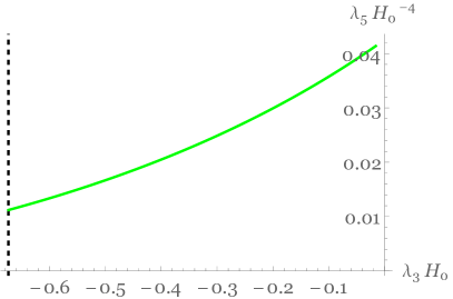
Figure 1: The one-dimensional parameter subspace of the $(\lambda_{3}-\lambda_{5})$ plane that satisfies the two phenomenological requirements, namely $H(z=0)\equiv H_{0}\approx 6\times 10^{-61}$ (in units where $8\pi G=c=\hbar=1$) and $w_{U}(z=0)\approx-0.7$. The dashed vertical line on the left marks the bound after which the two pathologies-absence conditions (13) and (14) are not satisfied.

In the left graph of Fig. 2 we present the solution for $H(z)$ from equation (37), for three choices of $\lambda_{3}$ and for comparison we additionally depict the corresponding evolution from the $\Lambda$CDM model. In the right graph of Fig. 2 we show the corresponding evolution for the total equation of state of the Universe from equation (IV), together with its evolution in the case of $\Lambda$CDM paradigm. Finally, for clarity in Fig. 3 we present $w_{U}(z)$ in logarithmic scale in order for the behaviour of larger $z$ to be visible.

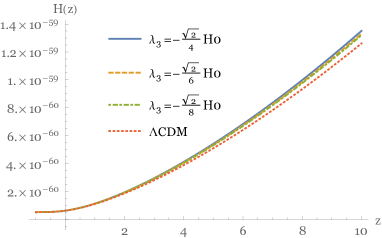
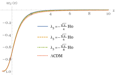
Figure 2: Left graph: The evolution of the Hubble parameter as a function of the redshift $z$, for the model (26), for various values of $\lambda_{3}$ in units where $8\pi G=c=\hbar=1$. We have set the present value of the total equation of state of the universe to $w_{U}(z=0)\approx-0.7$ and the present value of $H$ to $H_{0}\approx 6\times 10^{-61}$ which determines accordingly the value of $\lambda_{5}$ (see Fig. 1). Right graph: The corresponding evolution of $w_{U}(z)$. In both graphs we have added the corresponding curves of $\Lambda$CDM paradigm.

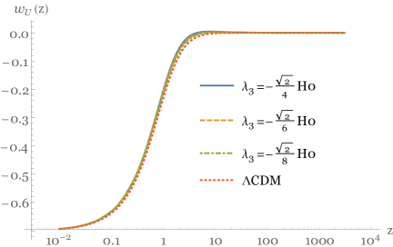
Figure 3: The evolution of $w_{U}(z)$ of the right graph of Fig. 2, in logarithmic scale up to $z\sim 3000$.

As we observe the form of $w_{U}(z)$ is in excellent agreement with observations. It is zero during the whole matter era, namely from redshifts $z\sim 3000$ up to $z\sim 2-3$, then it starts decreasing, passing the bound $-1/3$, which marks the onset of acceleration, at around $z\sim 0.5$, and finally it acquires a value $-0.7$ at present times (i.e at $z=0$). We mention that this behaviour is obtained without considering an explicit matter sector, namely it is the Galileon field itself that describes both the dark matter and dark energy sectors in a unified way. Furthermore, for completeness, in the same figures we have included the evolution up to the far future ($z\rightarrow-1$ corresponds to $t\rightarrow\infty$), where we can clearly see that the universe tends toward a de-Sitter phase. We stress that this de-Sitter phase is obtained although we have not considered an explicit cosmological constant, and hence it is a very interesting non-trivial result.

One can acquire a qualitative picture of the above results in the following way. If we manage to make $X$ to be almost constant at early times then we can expand $w_{U}$ from equation (31) for large $H$ (which is the case at early times) yielding an approximated value $w_{U}\rightarrow 0$. On the other hand, if $X$ departs from the constant value, acquiring a decreasing form, then $w_{U}$ starts deviating from 0 towards the $-1$ value. Our model (26) presents these behaviours, and indeed one can see that for large $H$ we obtain $X\rightarrow\frac{1}{3\lambda_{5}}=\text{constant}$ as requested. On the other hand, if we had included an extended non-minimal derivative coupling $\sim G_{5}(X)$ Harko:2016xip , then the introduced extra $\ddot{\phi}$ term would have changed the kinetic energy of the cosmological fluid spoiling the $w_{U}\rightarrow 0$ feature at early times, leading instead to $w_{U}\rightarrow const.$ However in that case, adding suitably more terms in the action one could realize the very interesting scenario that $w_{U}$ starts from $-1$ at very early times, then it departs towards $1/3$ remaining there for a sufficient time interval, then becoming zero for a very long time and finally departing towards $-1$ at late and future times. Such an evolution could describe the whole thermal history of the Universe, namely the inflationary, the radiation, the matter and finally the dark energy eras.

Let us now confront the model at hand with cosmological observations coming from Supernovae type Ia (SN Ia), which is straightforward as long as we have the evolution of $H(z)$. Observations measure the apparent luminosity vs redshift $l(z)$, or equivalently the apparent magnitude vs redshift $m(z)$, which are related to the luminosity distance by

$$2.5\log\left[\frac{L}{l(z)}\right]=\mu\equiv m(z)-M=5\log\left[\frac{d_{L}(z)_{\text{obs}}}{Mpc}\right]+25~{},$$ (39)

where $L$ and $M$ are respectively the absolute luminosity and magnitude. From the theory point of view the predicted Hubble parameter is related to the dimensionless luminosity distance $d_{L}(z)_{\text{th}}$ as

$$d_{L}\left(z\right)_{\text{th}}\equiv\left(1+z\right)\int^{z}_{0}\frac{dz^{\prime}}{H\left(z^{\prime}\right)}~{}.$$ (40)

In our model the evolution of $H(z)$ is given numerically from the differential equation (37), and it was presented in the left graph of Fig. 2. On the other hand, for the case of $\Lambda$CDM paradigm, the corresponding $H(z)$ is given by $H^{2}(z)=H_{0}^{2}\left[\Omega_{m0}(1+z)^{3}+\Omega_{\Lambda 0}\right]$, with $\Omega_{m}$ and $\Omega_{\Lambda}$ the matter and cosmological-constant density parameters respectively, and where the subscript “0” denotes the present value of these quantities. In Fig. 4 we present the theoretically predicted apparent minus absolute magnitude for the model (26), on top of the $580$ SN Ia data points from Suzuki:2011hu , as well as the corresponding curve from the $\Lambda$CDM scenario. As we observe, the agreement with the SN Ia data is excellent. The proposed model of dark matter - dark energy unification is almost indistinguishable from $\Lambda$CDM cosmology, although we have not considered an explicit cosmological constant and an explicit matter sector. This is one of the main results of the present work.

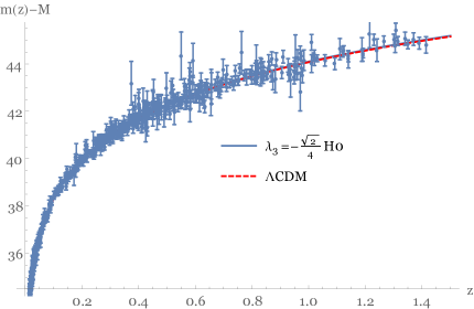
Figure 4: Theoretically predicted apparent minus absolute magnitude for the model (26), for $\lambda_{3}=-\sqrt{2}H_{0}/4$ in units where $8\pi G=c=\hbar=1$, on top of the $580$ SN Ia data points from Suzuki:2011hu . For comparison, we have added the corresponding curve of $\Lambda$CDM paradigm.

A comparison of the fittings of the above two scenarios can be achieved using the Akaike Information Criterion $(AIC)$ Akaike1974 . The $AIC$ is defined as

$$AIC=-2\ln\mathcal{L}+2d=\chi_{min}^{2}+2d,$$ (41)

with $\mathcal{L}=\exp\left(-\chi^{2}_{min}/2\right)$ the maximum likelihood function and $d$ the number of model parameters. The minimization of $\chi^{2}$ is defined as

$$\chi^{2}_{min}=\sum^{N}_{i}\frac{\left[\mu(z_{i})_{obs}-\mu(z_{i})_{th}\right]^{2}}{\sigma_{i}^{2}},$$ (42)

with $N=580$ the number of SN Ia contained in Suzuki:2011hu and $\sigma_{i}$ the error corresponding to each $\mu(z_{i})_{obs}$. The $\Lambda$CDM cosmology will be the reference scenario, with respect of which the comparison of the model under consideration will be performed. For any specific model $M$, calculating the difference $\Delta AIC={AIC}_{M}-{AIC}_{\Lambda\text{CDM}}$ and resulting to a value $\leq 2$, the considered model has substantial observational support with respect to the $\Lambda$CDM one Nunes:2016drj ; delaCruz-Dombriz:2016bqh . In the above analysis we have one parameter for $\Lambda$CDM paradigm, while in our model we have three free parameters. This results to a value

$$\Delta AIC=0.65<2,$$ (43)

and therefore the scenario at hand is very efficient concerning confrontation with observations.

To complete our analysis on the above scenario that describes in a unified way the dark matter and dark energy sectors, we must examine whether the model is free from pathologies such as ghosts and Laplacian instabilities at the perturbative level. Indeed, it is well known that in many modified gravities there appear various pathologies at the perturbative level, even if the background behaviour is problem-free and consistent. In the Horndeski theory, the two necessary conditions for absence of pathologies in the scalar perturbations are given in relations (13) and (14), which in the particular model of action (26) become

$$\!\!\!\!\!\!\!\!\!\!\!\!\!\!\!\!Q_{s}=-\frac{2(\lambda_{5}X-1)\Big{\{}3\lambda_{3}^{2}+6\sqrt{2}\lambda_{3}H(1-5\lambda_{5}X)+8X\left[\frac{1}{2}-\frac{1}{2}\lambda_{5}X+3\lambda_{5}H^{2}(1+3\lambda_{5}X)\right]\Big{\}}}{\left[\sqrt{2}\lambda_{3}+H(4-12\lambda_{5}X)\right]^{2}}>0~{},$$ (44)

$$\!\!\!\!\!\!\!\!\!\!\!\!\!\!c_{s}^{2}=\Big{\{}(\lambda_{5}X-1)\left\{3\lambda_{3}^{2}+6\sqrt{2}\lambda_{3}H(1-5\lambda_{5}X)+8X\left[\frac{1}{2}-\frac{1}{2}\lambda_{5}X+3\lambda_{5}H^{2}(1+3\lambda_{5}X)\right]\right\}\Big{\}}^{-1}$$

$$\cdot\Big{\{}32\lambda_{5}^{2}H^{2}X^{2}(3\lambda_{5}X-1)-8(\lambda_{5}X-1)^{2}(3\lambda_{5}X-1)\dot{H}+\lambda_{3}\left[\lambda_{3}+\lambda_{3}\lambda_{5}X-4\sqrt{2}\lambda_{5}(\lambda_{5}X-1)\dot{X}\right]$$

$$\ \ \ -2H\left\{\sqrt{2}\lambda_{3}\left[\lambda_{5}X(2+7\lambda_{5}X)-1\right]-4\lambda_{5}(\lambda_{5}X-1)(1+3\lambda_{5}X)\dot{X}\right\}\Big{\}}\geq 0~{},$$ (45)

with the additional constraint $c_{s}^{2}\leq 1$. These conditions must be valid on-shell of the background evolution and at all times.

In Fig. 5 we present the evolution of $Q_{s}$ and $c_{s}^{2}$ for the background evolution and parameter choices of Fig. 2. We observe that the conditions for absence of ghosts and Laplacian instabilities are always satisfied, and thus the scenario at hand is free from pathologies of the scalar sector at both background and perturbative level. We mention here that although the desired background evolution can be relatively easily obtained with an action of the form (1), to satisfy the pathologies-absence conditions requires careful selection of the involved functions. Hence, as we mentioned earlier, in the particular model (26) the choice of $X^{1/2}$ in the specific forms of $K(\phi,X)$ and $G_{3}(\phi,X)$ is not necessary for obtaining the desired phenomenological evolution at the background level, however it is important in order to make $c_{s}^{2}$ positive at all times, since the Cuscuton and the Kinetic Gravity Braiding terms (which exhibit superluminal sound speed) ensure that the sound speed square will increase and avoid negative values.

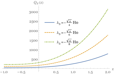
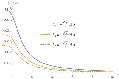
Figure 5: Left graph: The evolution of $Q_{s}$ from (44), that characterizes the absence of Laplacian instabilities, as a function of the redshift $z$, for the model (26), for various values of $\lambda_{3}$ in units where $8\pi G=c=\hbar=1$. We have set the present value of the total equation of state of the universe to $w_{U}(z=0)\approx-0.7$ and the present value of $H$ to $H_{0}\approx 6\times 10^{-61}$. Right graph: The corresponding evolution of the sound speed square of the scalar perturbations $c_{s}^{2}$ from (45).

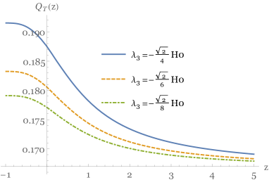
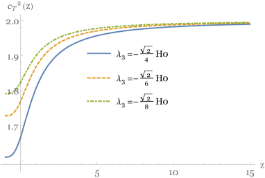
Figure 6: Left graph: The evolution of $Q_{T}$ from (46), that characterizes the absence of Laplacian instabilities, as a function of the redshift $z$, for the model (26), for various values of $\lambda_{3}$ in units where $8\pi G=c=\hbar=1$. We have set the present value of the total equation of state of the universe to $w_{U}(z=0)\approx-0.7$ and the present value of $H$ to $H_{0}\approx 6\times 10^{-61}$. Right graph: The corresponding evolution of the sound speed square of the tensor perturbations $c_{T}^{2}$ from (47).

Finally, concerning tensor perturbations, the two necessary conditions for absence of ghost and Laplacian instabilities are given in (19) and (20), and thus in the particular model of action (26) become

$$Q_{T}=\frac{1}{4}(1-\lambda_{5}X)$$ (46)

$$c_{T}^{2}=\frac{\lambda_{5}X+1}{1-\lambda_{5}X}\geq 0.$$ (47)

In Fig. 6 we depict the evolution of $Q_{T}$ and $c_{T}^{2}$ for the background evolution and parameter choices of Fig. 2. As we can see, the conditions for absence of ghosts and Laplacian instabilities are always satisfied, and thus the scenario at hand is free from pathologies in the tensor sector too. Additionally, note that since the specific model considered here contains $G_{5}$, the tensor perturbations may become superluminal, as expected DeFelice:2011bh ; Germani:2010ux . However, as discussed above, this feature does not imply pathologies or acausality Babichev:2007dw ; Deffayet:2010qz .

V Conclusions

In this work we have presented a unified description of the dark matter and dark energy sectors, in the framework of shift-symmetric generalized Galileon theories. Although in usual applications of Galileon/Horndeski theories one includes the extra scalar degree of freedom in order to represent the inflaton or the dark-energy field, while the matter sector is considered additionally, in our approach we used this scalar field in order to account for both dark matter and dark energy sectors simultaneously. Using a specific combination of terms of the Galileon/Horndeski Lagrangian, and without considering an explicit matter sector and an explicit cosmological constant, we obtained an effective cosmic fluid that behaves as pressureless matter during the matter era, and as dark energy at late times, thus producing a unified description of the cosmological evolution.

In particular, the shift symmetry imposed on the action allowed the derivation of the pressure of the effective fluid as a function of the energy density, namely $p_{U}=p_{U}(\rho_{U})$, which proves to have the form of an extended Chaplygin gas. Chaplygin gas has been known to be efficient in offering a unified description of the matter and dark energy regimes. In the present model the generalized equation of state parameter for the unified fluid $w_{U}$ is acquired straightaway from the action considered.

The obtained behaviour of $w_{U}(z)$ is in excellent agreement with observations. It is zero during the whole matter era, namely from redshifts $z\sim 3000$ up to $z\sim 2-3$, then it starts decreasing, passing the bound $-1/3$, which marks the onset of acceleration, at around $z\sim 0.5$, and finally it acquires a value $-0.7$ at present times. Additionally, confronting this evolution with the Supernovae type Ia data we showed that we obtained an excellent fit, and our model of dark-matter - dark-energy unification is almost indistinguishable from $\Lambda$CDM cosmology. Moreover, investigating the evolution up to the far future we saw that the universe tends toward a de-Sitter phase. We stress that these behaviours are obtained without considering an explicit matter sector or an explicit cosmological constant, namely it is the Galileon field itself that describes both the dark matter and dark energy sectors in a unified way. This is the main result of the present work.

Finally, we examined in detail the behaviour of the above unified scenario at the perturbative level, focusing on the conditions of absence of pathologies such as ghosts and Laplacian instabilities, at both scalar and tensor sectors. This is a crucial step that must be taken in every cosmological application, since it is well known that in many modified theories of gravities there appear various pathologies at the perturbative level, even if the background behaviour is problem-free and consistent. We showed that with the consideration of specific terms in the action the various pathologies-absence conditions are satisfied at all times on top of the background unified solutions.

As a further work on this unification approach of the dark sectors it would be interesting to consider the powerful method of dynamical system analysis in order to bypass the nonlinearities of the equations and extract the global features and the asymptotic behaviour of the evolution. Furthermore, apart from the SN Ia data, one should use observations from Baryon Acoustic Oscillations (BAO), from Cosmic Microwave Background (CMB), and from Large Scale Structure (LSS), in order to obtain a more detailed and complete confrontation, since this was the weak point of previously constructed unified scenarios such as the Chaplygin gas. Additionally, one should try to focus on solutions where the scalar-field kinetic energy becomes very small, at least in the late-time universe, in order for the tensor perturbation speed to get reduced close to the light speed. In order to pass these necessary observational comparisons one must consider the baryonic matter sector explicitly, since this will not affect the obtained unified description of the dark matter and dark energy sectors.

References

- (1) S. Perlmutter et al. [Supernova Cosmology Project Collaboration], “Discovery of a supernova explosion at half the age of the Universe and its cosmological implications,” Nature 391, 51 (1998) [astro-ph/9712212].
- (2) A. G. Riess et al. [Supernova Search Team], “Observational evidence from supernovae for an accelerating universe and a cosmological constant,” Astron. J. 116, 1009 (1998) [astro-ph/9805201].
- (3) E. J. Copeland, M. Sami and S. Tsujikawa, “Dynamics of dark energy,” Int. J. Mod. Phys. D 15, 1753 (2006) [hep-th/0603057].
- (4) A. Joyce, B. Jain, J. Khoury and M. Trodden, “Beyond the Cosmological Standard Model,” Phys. Rept. 568, 1 (2015) [arXiv:1407.0059 [astro-ph.CO]].
- (5) B. Wang, E. Abdalla, F. Atrio-Barandela and D. Pavon, “Dark Matter and Dark Energy Interactions: Theoretical Challenges, Cosmological Implications and Observational Signatures,” Rept. Prog. Phys. 79, no. 9, 096901 (2016) [arXiv:1603.08299 [astro-ph.CO]].
- (6) Y. L. Bolotin, A. Kostenko, O. A. Lemets and D. A. Yerokhin, “Cosmological Evolution With Interaction Between Dark Energy And Dark Matter,” Int. J. Mod. Phys. D 24, no. 03, 1530007 (2014) [arXiv:1310.0085 [astro-ph.CO]].
- (7) M. C. Bento, O. Bertolami and A. A. Sen, “Generalized Chaplygin gas, accelerated expansion and dark energy matter Phys. Rev. D 66, 043507 (2002). [gr-qc/0202064].
- (8) M. d. C. Bento, O. Bertolami and A. A. Sen, “Generalized Chaplygin gas and CMBR constraints,” Phys. Rev. D 67, 063003 (2003) [astro-ph/0210468].
- (9) M. C. Bento, O. Bertolami, M. J. Reboucas and P. T. Silva, “Generalized Chaplygin gas model, supernovae and cosmic topology,” Phys. Rev. D 73, 043504 (2006) [gr-qc/0512158].
- (10) H. Sandvik, M. Tegmark, M. Zaldarriaga and I. Waga, “The end of unified dark matter?,” Phys. Rev. D 69, 123524 (2004) [astro-ph/0212114].
- (11) M. U. Farooq, M. Jamil and M. A. Rashid, “Interacting entropy-corrected holographic Chaplygin gas model,” Int. J. Theor. Phys. 49, 2334 (2010) [arXiv:1003.3399 [gr-qc]].
- (12) V. Gorini, A. Y. Kamenshchik, U. Moschella, O. F. Piattella and A. A. Starobinsky, “Gauge-invariant analysis of perturbations in Chaplygin gas unified models of dark matter and dark energy,” JCAP 0802, 016 (2008) [arXiv:0711.4242 [astro-ph]].
- (13) U. Debnath, A. Banerjee and S. Chakraborty, “Role of modified Chaplygin gas in accelerated universe,” Class. Quant. Grav. 21, 5609 (2004) [gr-qc/0411015].
- (14) M. Bouhmadi-Lopez and P. Vargas Moniz, “FRW quantum cosmology with a generalized Chaplygin gas,” Phys. Rev. D 71, 063521 (2005) [gr-qc/0404111].
- (15) M. R. Setare, “Interacting holographic generalized Chaplygin gas model,” Phys. Lett. B 654, 1 (2007) [arXiv:0708.0118 [hep-th]].
- (16) Y. Fujii and K. Maeda, The scalar-tensor theory of gravitation, Cambridge University Press, Cambridge (2003).
- (17) G. W. Horndeski, “Second-order scalar-tensor field equations in a four-dimensional space,” Int. J. Theor. Phys. 10 (1974) 363.
- (18) M. Ostrogradsky, “Mémoires sur les équations différentielles, relatives au problème des isopérimètres”, Mem. Acad. St. Petersbourg 6, no. 4, 385 (1850).
- (19) A. Nicolis, R. Rattazzi, E. Trincherini, “The Galileon as a local modification of gravity,” Phys. Rev. D79 (2009) 064036 [arXiv:0811.2197 [hep-th]].
- (20) C. Deffayet, G. Esposito-Farese, A. Vikman, “Covariant Galileon,” Phys. Rev. D79 (2009) 084003 [arXiv:0901.1314 [hep-th]].
- (21) C. Deffayet, S. Deser and G. Esposito-Farese, “Generalized Galileons: All scalar models whose curved background extensions maintain second-order field equations and stress-tensors,” Phys. Rev. D 80, 064015 (2009) [arXiv:0906.1967].
- (22) C. Deffayet, X. Gao, D. A. Steer and G. Zahariade, “From k-essence to generalised Galileons,” Phys. Rev. D 84 (2011) 064039 [arXiv:1103.3260 [hep-th]].
- (23) A. I. Vainshtein, “To the problem of nonvanishing gravitation mass,” Phys. Lett. B 39, 393 (1972).
- (24) N. Chow and J. Khoury, “Galileon Cosmology,” Phys. Rev. D 80, 024037 (2009) [arXiv:0905.1325]].
- (25) A. De Felice, R. Kase and S. Tsujikawa, “Vainshtein mechanism in second-order scalar-tensor theories,” Phys. Rev. D 85, 044059 (2012) [arXiv:1111.5090]].
- (26) E. Babichev, C. Deffayet and G. Esposito-Farese, “Improving relativistic MOND with Galileon k-mouflage,” Phys. Rev. D 84, 061502 (2011) [arXiv:1106.2538]].
- (27) E. N. Saridakis and M. Tsoukalas, “Cosmology in new gravitational scalar-tensor theories,” Phys. Rev. D 93, no. 12, 124032 (2016) [arXiv:1601.06734 [gr-qc]].
- (28) C. de Rham and L. Heisenberg, “Cosmology of the Galileon from Massive Gravity,” Phys. Rev. D 84, 043503 (2011) [arXiv:1106.3312 [hep-th]].
- (29) L. Heisenberg, R. Kimura and K. Yamamoto, “Cosmology of the proxy theory to massive gravity,” Phys. Rev. D 89, 103008 (2014) [arXiv:1403.2049 [hep-th]].
- (30) M. Rinaldi, “Mimicking dark matter in Horndeski gravity,” Phys. Dark Univ. 16, 14 (2017). [arXiv:1608.03839 [gr-qc]].
- (31) A. De Felice and S. Tsujikawa, “Generalized Galileon cosmology,” Phys. Rev. D 84, 124029 (2011) [arXiv:1008.4236]].
- (32) A. De Felice and S. Tsujikawa, “Conditions for the cosmological viability of the most general scalar-tensor theories and their applications to extended Galileon dark energy models,” JCAP 1202, 007 (2012) [arXiv:1110.3878]].
- (33) A. De Felice and S. Tsujikawa, “Cosmology of a covariant Galileon field,” Phys. Rev. Lett. 105, 111301 (2010) [arXiv:1007.2700]].
- (34) S. A. Appleby and E. V. Linder, “The Paths of Gravity in Galileon Cosmology,” JCAP 1203, 043 (2012) [arXiv:1112.1981 [astro-ph.CO]].
- (35) E. Babichev, V. Mukhanov and A. Vikman, “k-Essence, superluminal propagation, causality and emergent geometry,” JHEP 0802, 101 (2008) arXiv:0708.0561 [hep-th]].
- (36) C. Deffayet, O. Pujolas, I. Sawicki and A. Vikman, “Imperfect Dark Energy from Kinetic Gravity Braiding,” JCAP 1010, 026 (2010) [arXiv:1008.0048 [hep-th]].
- (37) A. Adams, N. Arkani-Hamed, S. Dubovsky, A. Nicolis and R. Rattazzi, “Causality, analyticity and an IR obstruction to UV completion,” JHEP 0610, 014 (2006) [hep-th/0602178].
- (38) D. A. Easson, I. Sawicki and A. Vikman, “When Matter Matters,” JCAP 1307, 014 (2013) [arXiv:1304.3903 [hep-th]].
- (39) P. A. R. Ade et al. [Planck Collaboration], “Planck 2015 results. XIII. Cosmological parameters,” Astron. Astrophys. 594, A13 (2016) [arXiv:1502.01589 [astro-ph.CO]].
- (40) L. Amendola, “Cosmology with nonminimal derivative couplings,” Phys. Lett. B 301, 175 (1993) [gr-qc/9302010].
- (41) T. Kolyvaris, G. Koutsoumbas, E. Papantonopoulos and G. Siopsis, “Scalar Hair from a Derivative Coupling of a Scalar Field to the Einstein Tensor,” Class. Quant. Grav. 29, 205011 (2012), [arXiv:1111.0263 [gr-qc]].
- (42) M. Rinaldi, “Black holes with non-minimal derivative coupling,” Phys. Rev. D 86, 084048 (2012) [arXiv:1208.0103 [gr-qc]].
- (43) T. Kolyvaris, G. Koutsoumbas, E. Papantonopoulos and G. Siopsis, “Phase Transition to a Hairy Black Hole in Asymptotically Flat Spacetime,” JHEP 1311, 133 (2013), [arXiv:1308.5280 [hep-th]].
- (44) G. Koutsoumbas, K. Ntrekis, E. Papantonopoulos and M. Tsoukalas, “Gravitational Collapse of a Homogeneous Scalar Field Coupled Kinematically to Einstein Tensor,” Phys. Rev. D 95, no. 4, 044009 (2017) [arXiv:1512.05934 [gr-qc]].
- (45) S. V. Sushkov, “Exact cosmological solutions with nonminimal derivative coupling,” Phys. Rev. D 80, 103505 (2009) [arXiv:0910.0980 [gr-qc]].
- (46) C. Gao, “When scalar field is kinetically coupled to the Einstein tensor,” JCAP 1006, 023 (2010) [arXiv:1002.4035 [gr-qc]].
- (47) L. N. Granda, “Non-minimal Kinetic coupling to gravity and accelerated expansion,” JCAP 1007, 006 (2010) [arXiv:0911.3702 [hep-th]].
- (48) E. N. Saridakis and S. V. Sushkov, “Quintessence and phantom cosmology with non-minimal derivative coupling,” Phys. Rev. D 81, 083510 (2010) [arXiv:1002.3478 [gr-qc]].
- (49) C. Germani, A. Kehagias, “New Model of Inflation with Non-minimal Derivative Coupling of Standard Model Higgs Boson to Gravity,” Phys. Rev. Lett. 105, 011302 (2010) [arXiv:1003.2635 [hep-ph]].
- (50) J. B. Dent, S. Dutta, E. N. Saridakis and J. Q. Xia, “Cosmology with non-minimal derivative couplings:perturbation analysis and observational constraints,” JCAP 1311, 058 (2013) [arXiv:1309.4746 [astro-ph.CO]].
- (51) I. Dalianis, G. Koutsoumbas, K. Ntrekis and E. Papantonopoulos, “Reheating predictions in Gravity Theories with Derivative Coupling,” JCAP 1702, no. 02, 027 (2017) [arXiv:1608.04543 [gr-qc]].
- (52) G. Koutsoumbas, K. Ntrekis and E. Papantonopoulos, “Gravitational Particle Production in Gravity Theories with Non-minimal Derivative Couplings,” JCAP 1308, 027 (2013), [arXiv:1305.5741 [gr-qc]].
- (53) X. M. Kuang and E. Papantonopoulos, “Building a Holographic Superconductor with a Scalar Field Coupled Kinematically to Einstein Tensor,” JHEP 1608, 161 (2016), [arXiv:1607.04928 [hep-th]].
- (54) C. Bogdanos and E. N. Saridakis, “Perturbative instabilities in Horava gravity,” Class. Quant. Grav. 27, 075005 (2010) [arXiv:0907.1636 [hep-th]].
- (55) A. De Felice, A. E. Gumrukcuoglu and S. Mukohyama, “Massive gravity: nonlinear instability of the homogeneous and isotropic universe,” Phys. Rev. Lett. 109, 171101 (2012) [arXiv:1206.2080 [hep-th]].
- (56) N. Afshordi, D. J. H. Chung and G. Geshnizjani, “Cuscuton: A Causal Field Theory with an Infinite Speed of Sound,” Phys. Rev. D 75, 083513 (2007) [hep-th/0609150].
- (57) M. C. Bento, O. Bertolami and A. A. Sen, “WMAP Constraints on the Generalized Chaplygin Gas Model,” Phys. Lett. B 575, 172 (2003) [arXiv:astro-ph/0303538].
- (58) A. Y. Kamenshchik, U. Moschella and V. Pasquier, “An Alternative to quintessence,” Phys. Lett. B 511, 265 (2001) [gr-qc/0103004].
- (59) V. Gorini, A. Kamenshchik, U. Moschella, V. Pasquier and A. Starobinsky, Phys. Rev. D 72, 103518 (2005) [astro-ph/0504576].
- (60) L. N. Granda, E. Torrente-Lujan and J. J. Fernandez-Melgarejo, “Non-minimal kinetic coupling and Chaplygin gas cosmology,” Eur. Phys. J. C 71, 1704 (2011) [arXiv:1106.5482 [hep-th]].
- (61) C. Armendariz-Picon, V. F. Mukhanov and P. J. Steinhardt, “A Dynamical solution to the problem of a small cosmological constant and late time cosmic acceleration,” Phys. Rev. Lett. 85, 4438 (2000) [astro-ph/0004134].
- (62) O. Pujolas, I. Sawicki and A. Vikman, “The Imperfect Fluid behind Kinetic Gravity Braiding,” JHEP 1111, 156 (2011) [arXiv:1103.5360 [hep-th]].
- (63) T. Harko, F. S. N. Lobo, E. N. Saridakis and M. Tsoukalas, “Cosmological models in modified gravity theories with extended nonminimal derivative couplings,” Phys. Rev. D 95, no. 4, 044019 (2017) [arXiv:1609.01503 [gr-qc]].
- (64) N. Suzuki et al., “The Hubble Space Telescope Cluster Supernova Survey: V. Improving the Dark Energy Constraints Above z1 and Building an Early-Type-Hosted Supernova Sample,” Astrophys. J. 746, 85 (2012) [arXiv:1105.3470 [astro-ph.CO]].
- (65) H. Akaike, “A new look at the statistical model identification”, IEEE Transactions on Automatic Control, 19, 716 (1974).
- (66) R. C. Nunes, S. Pan, E. N. Saridakis and E. M. C. Abreu, “New observational constraints on gravity from cosmic chronometers,” JCAP 1701, no. 01, 005 (2017) [arXiv:1610.07518 [astro-ph.CO]].
- (67) A. de la Cruz-Dombriz, P. K. S. Dunsby, O. Luongo and L. Reverberi, “Model-independent limits and constraints on extended theories of gravity from cosmic reconstruct ion techniques,” JCAP 1612, no. 12, 042 (2016) [arXiv:1608.03746 [gr-qc]].
- (68) C. Germani and A. Kehagias, “Cosmological Perturbations in the New Higgs Inflation,” JCAP 1005, 019 (2010) [arXiv:1003.4285 [astro-ph.CO]].
- (69) B. P. Abbott et al. [LIGO Scientific and Virgo Collaborations], “GW170817: Observation of Gravitational Waves from a Binary Neutron Star Inspiral,” Phys. Rev. Lett. 119, no. 16, 161101 (2017) [arXiv:1710.05832 [gr-qc]].
- (70) B. P. Abbott et al. [LIGO Scientific and Virgo and Fermi-GBM and INTEGRAL Collaborations], “Gravitational Waves and Gamma-Rays from a Binary Neutron Star Merger: GW170817 and GRB 170817A,” Astrophys. J. 848, no. 2, L13 (2017) [arXiv:1710.05834 [astro-ph.HE]].
- (71) J. M. Ezquiaga and M. Zumalacárregui, “Dark Energy after GW170817,” Phys. Rev. Lett. 119, no. 25, 251304 (2017) [arXiv:1710.05901 [astro-ph.CO]].
- (72) T. Baker, E. Bellini, P. G. Ferreira, M. Lagos, J. Noller and I. Sawicki, “Strong constraints on cosmological gravity from GW170817 and GRB 170817A,” Phys. Rev. Lett. 119, no. 25, 251301 (2017) [arXiv:1710.06394 [astro-ph.CO]].