Second law for an autonomous information machine connected with multiple baths

Abstract

In an Information machine system’s dynamics gets affected by the attached information reservoir. Second law of thermodynamics can be apparently violated for this case. In this article we have derived second law for an information machine, when the system is connected to multiple heat baths along with a work source and a single information reservoir. Here a sequence of bits written on a tape is considered as an information reservoir. We find that the bath entropy production during a time interval is restricted by the change of Shannon entropy of the composite system (system + information reservoir) during that interval. We have also given several examples where this law can be applicable and shown that our bound is tighter.

Keywords: information processing, exact results, stochastic processes

1 Introduction

Second law is a fundamental law in thermodynamics and always valid on an average [1, 2, 3]. According to the law average entropy production is always positive. Recent development of fluctuation theorems dictates that it is possible to find negative entropy production for an individual event for any duration although their probabilities are exponentially small. However validity of the second law was questioned by Maxwell even more than a century ago, when he proposed a thought experiment involving an intelligent being known as Maxwell demon [4]. In this gedanken experiment only by knowing the velocity of gas particles confined in a box, a demon can separate them into hotter (consists of faster molecules) and colder (consists of slower molecules) part without doing any work. Half a century later, Szilard proposed another thought experiment [5] where he showed that it is always possible to extract heat from single heat bath and perform useful work cyclically when a gas molecule, confined in a box, is treated by a certain protocol which involves measurement of the state of the system.

To understand these puzzles, the last century has witnessed several wonderful research works establishing the connection between information theory and thermodynamics. [6, 7, 8, 9, 10, 11, 12, 13, 14, 15, 16]. In fact one needs to take into account the cost of information during the process and above all, the process would be completed only when the information contained in the memory register of the demon will be erased. Now, according to Landauer[6], one need to do at least $k_{B}T\ln 2$ work to erase one bit of information ($k_{B}$ represents Boltzmann constant). Hence the second law is saved when one takes into account the effect of information.

There are mainly two cases in the framework of information processing when the second law is apparently violated [13, 14]. In the first one, measurement is performed and depending on the measurement outcome, the protocol is altered. In another approach, the information contained in an information reservoir is changed when it is allowed to interact sequentially with the system [11, 17, 18]. A sequence of bits written on a tape can be considered as an information reservoir. Recently the second type of approach draws many attention and second law has been derived consequently[17, 19, 20, 21, 22]. The performance of autonomous information machine has been explained just taking bath entropy production restricted by the configuration entropy change of the tape[12, 13, 11, 17, 18]. However the inequality should contain the correlation between demon and tape which makes the inequality stronger[17]. In [19, 20] it is shown that the work done is bounded by the change in Kolmogorov-Sinai dynamical entropy rate of the tape when system is connected to a heat bath, a work source and an information reservoir(tape). Here, the derivation is done by taking into account the correlations within the input string and those in the output string generated during its evolution connecting with the demon. Note that, this bound is stronger when input is uncorrelated or the system(ratchet or demon) is memoryless (i.e., it has no internal states), compared to the earlier version [12, 13, 11] where statistical correction between the bits are neglected and work is bounded by the marginal configuration Shannon entropy of the individual bits. Although the result is generally valid even when input is correlated and the ratchet has memory there is some concern as discussed in [22]. Besides the second law is derived in [22] exactly in a straight forward way by simply adding the inequalities for each individual cycles. When a system is connected to a heat bath, a work source and an information reservoir, the corresponding second law for single cycle is given by

$$\beta W\leq\mathcal{H}(\Pi_{\tau})-\mathcal{H}(\Pi_{0}).$$ (1)

Here $\mathcal{H}$ represents the Shannon entropy of the joint system consisting of interacting bit and system. If that joint distribution at any time t is given by $\Pi_{t}$ then corresponding Shannon entropy is denoted by $\mathcal{H}(\Pi_{t})=-\sum\Pi_{t}\ln\Pi_{t}$ where the sum is done over all possible states. The above equation dictates that the average extracted work $W$ during the time interval $0\leq t<\tau$ is restricted by the change of Shannon entropy of the joint system during that interval. Motivated by this, we would like to study an information machine which is connected to multiple baths. We have obtained corresponding second law which is exact and most general as well as the bound is more compact. The derivation here is done by scrutinizing how an autonomous information machine processed a tape sequentially during its operation. Moreover the obtained inequality reduced to the earlier results in spacial cases. The organization of the paper is as follows. First we describe the model and derive our result. Then we compare the result with the earlier studies. After that we give several examples where this law can be applicable. Finally taking a simple model, we numerically showed that our bound is stronger.

2 The Model

The model consists of a demon(system) which is attached with an information reservoir and a work source. A tape, where the information is written as discrete symbols, acts as an information reservoir. The input tape is formed by a sequence of symbols $x_{1}$,$x_{2}$,$x_{3}$,…,$x_{N}$ which is taken from a finite set $\chi$ (for binary symbols $\chi=(0,1)$). Each symbol interacts one by one sequentially with the demon. As a result, the demon state is going through internal states $s_{1}$, $s_{2}$, $s_{3},...,s_{N}$ which is taken from a finite set $S$. On the other hand, after interaction, the outgoing tape consists of another sequence of symbols $y_{1}$,$y_{2}$,$y_{3}$,…,$y_{N}$ which are elements of same set $\chi$. Note that there are no intrinsic transitions in the tape. Only during its interaction with the demon the tape state may change. The total entropy of the incoming tape is given by

$$H(X^{N})=-\sum_{x^{N}\in\chi}P(x^{N})\ln P(x^{N}).$$ (2)

Here, $P(x^{N})=P(x_{1},x_{2},x_{3},...,x_{N})$ is the probability distribution of that sequence of the input. Now, If the input sequence is correlated then

$$H(X^{N}) =-\sum_{x^{N}\in\chi}P(x^{N})\ln P(x^{N})$$ (3)

$$=-\sum_{x^{N}\in\chi}P(x^{N})\ln\left[P(x_{N}|x^{N-1})......P(x_{3}|x_{2},x_{1})P(x_{2}|x_{1})P(x_{1})\right]$$

$$=-\sum_{x^{N}\in\chi}P(x^{N})\ln P(x_{N}|x^{N-1})-.....-\sum_{x^{N}\in\chi}P(x^{N})\ln P(x_{3}|x_{2},x_{1})$$

$$\hskip 85.35826pt-\sum_{x^{N}\in\chi}P(x^{N})\ln P(x_{2}|x_{1})-\sum_{x^{N}\in\chi}P(x^{N})\ln P(x_{1})$$

$$=-\sum_{x^{N}}P(x^{N})\ln P(x_{N}|x^{N-1})-.....-\sum_{x_{3},x_{2},x_{1}}P(x_{3},x_{2},x_{1})\ln P(x_{3}|x_{2},x_{1})$$

$$\hskip 85.35826pt-\sum_{x_{2},x_{1}}P(x_{2},x_{1})\ln P(x_{2}|x_{1})-\sum_{x_{1}}P(x_{1})\ln P(x_{1})$$

$$=\sum_{n=1}^{N}H(X_{n}|X^{n-1}).$$

Where $H(X_{n}|X^{n-1})=-\sum_{x^{n}}P(x^{n})\ln P(x_{n}|x^{n-1})$. Similarly if $P(y^{N})=P(y_{1},y_{2},y_{3},...,y_{N})$ represents the probability distribution of the output sequence of the tape, then its entropy is given by

$$H(Y^{N})=-\sum_{y^{N}\in\chi}P(y^{N})\ln P(y^{N})=\sum_{n=1}^{N}H(Y_{n}|Y^{n-1}).$$ (4)

The demon can interact with the nearest symbol of the tape at a time. Now if the tape moves with constant speed $v$ then each symbol gets $\tau$ time to interact, after that the next symbol arrives. During that time, the joint state of demon and tape evolves with time. As an example, in $n^{th}$ interaction interval in between time $(n-1)\tau\leq t<n\tau$, the input joint state $(x_{n},s_{n})$ evolves and finally reaches to $(y_{n},s_{n+1})$. In the beginning of the next cycle, the demon state does not change but the tape is advanced by one unit. As a result the next cycle starts from the joint state $(x_{n+1},s_{n+1})$. After time $\tau$, the state $(x_{n+1},s_{n+1})$ evolves to $(y_{n+1},s_{n+2})$ and this process continues until the tape passes completely.

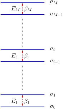
Figure 1: Schematic diagram to describe the joint states of demon and information reservoir. The energy difference between the states $\sigma_{i}$ and $\sigma_{i-1}$ is denoted by $E_{i}$ and when transition occurs between these states, energy is exchanged only with the bath having inverse temperature $\beta_{i}$,

Note that there is two types of dynamics. One is discrete and only deals with the input and output states ( $(x_{1},s_{1})\rightarrow(y_{1},s_{2});(x_{2},s_{2})\rightarrow(y_{2},s_{3});....$ ). Another one is continuous and deals how a output state is evolved from the input state during the time interval $\tau$. Consider the states of the composite system of demon and interacting tape are taken form a product set ($\chi\times S$) that contains M + 1 elements which are denoted by $(\sigma_{0},\sigma_{1},.....,\sigma_{M})$. Now at the starting of $n^{th}$ cycle the input state is related to the joint state by $(x_{n},s_{n})\equiv\sigma^{(n-1)\tau}$. Note that the superscript only denotes the time at which the state appears. The state $\sigma^{(n-1)\tau}$ then evolves according to the dynamics and finally at $n\tau^{-}$ it reaches to another element, say $\sigma^{n\tau^{-}}\equiv(y_{n},s_{n+1})$. At time $n\tau$ the tape is forwarded by one unit and the bit state is changed. As a result, the next cycle starts from $(x_{n+1},s_{n+1})\equiv\sigma^{n\tau}$ which is again an element of that set and the process continues. It can be mentioned that if the output and next input symbol (bit for binary sequence) is same then the actual state does not change at the time of this switching, if not, then it starts from another element of $\sigma$. Next we will describe the dynamics and the evolution of the joint system in a particular interval in detail.

3 Derivation of Second Law in presence of multiple baths

The energy difference between the states $\sigma_{0}$ and $\sigma_{1}$ is $E_{1}$ (fig.1). Similarly for $\sigma_{1}$ and $\sigma_{2}$ it is $E_{2}$ and so on. Note that, we have taken $\sigma_{0}$ as ground state and corresponding energy is taken as 0. Each of these consecutive states can exchange energy with only one bath and transition can only happen between the consecutive states. As an example, transition between $\sigma_{0}$ and $\sigma_{1}$ can only happen by exchanging heat from a bath with inverse temperature $\beta_{1}$. Hence corresponding transition rates satisfy the required detailed balance [23]

$$\frac{R_{\sigma_{0}\rightarrow\sigma_{1}}}{R_{\sigma_{1}\rightarrow\sigma_{0}}}=\exp^{-\beta_{1}E_{1}}.$$ (5)

Similarly for $\sigma_{1}$ and $\sigma_{2}$ the transition can happen when heat is exchanged from the bath with inverse temperature $\beta_{2}$ and corresponding transition rates satisfy detailed balance

$$\frac{R_{\sigma_{1}\rightarrow\sigma_{2}}}{R_{\sigma_{2}\rightarrow\sigma_{1}}}=\exp^{-\beta_{2}E_{2}},$$ (6)

and so on. Note that according to the construction of the model there is no other transition possible from or to $\sigma_{1}$. Moreover, the network of all the states form a linear chain and only back and forth excursions (transitions) along the chain is possible.

During any time interval $\tau$, the probability distribution of joint states of demon and bits $\Pi_{t}(\sigma)$ evolves according to the master equation

$$\frac{d\Pi_{t}(\sigma)}{dt}=\mathcal{R}\Pi_{t}({\sigma}),$$ (7)

where $\mathcal{R}$ denotes the transition rate matrix whose elements are $R_{\sigma_{i}\rightarrow\sigma_{j}}$. At $\tau\rightarrow\infty$ the composite system eventually reaches to the steady state where the probability distribution does not alter with time and can be determined easily taking $\mathcal{R}\Pi_{s}({\sigma})=0$. Now according to the construction of the model, those steady state probability distributions of two successive levels are related by

$\Pi_{s}(\sigma_{1})=\exp^{-\beta_{1}E_{1}}\Pi_{s}(\sigma_{0})$,

$\Pi_{s}(\sigma_{2})=\exp^{-\beta_{2}E_{2}}\Pi_{s}(\sigma_{1})$,

$\Pi_{s}(\sigma_{3})=\exp^{-\beta_{3}E_{3}}\Pi_{s}(\sigma_{2})$,

and so on. Therefore the steady state distribution for any state ($\sigma_{i}$) can be written as

$$\Pi_{s}(\sigma_{i}) =\exp^{-\beta_{i}E_{i}}\Pi_{s}(\sigma_{i-1})$$ (8)

$$=\exp^{-(\beta_{i}E_{i}+.....+\beta_{2}E_{2}+\beta_{1}E_{1})}\Pi_{s}(\sigma_{0})$$

$$=\frac{e^{-\sum_{j=1}^{i}\beta_{j}E_{j}}}{Z}.$$

Where in the last line, we have used the normalization condition and $Z=1+\sum_{i=1}^{M}e^{-\sum_{j=1}^{i}\beta_{j}E_{j}}$. It is well known that as time passes, $\Pi_{t}$ (the probability density at any time t) will approach monotonically towards $\Pi_{s}$ and their distance will reduce (Here for notational simplicity we have taken $0\leq t<\tau$. However it will be true for any interval $(n-1)\tau\leq t<n\tau$). Hence one can write [24]

$$D(\Pi_{\tau}||\Pi_{s})\leq D(\Pi_{0}||\Pi_{s}).$$ (9)

Here the Kullback-Leibler divergence is defined as $D(\Pi_{t_{1}}||\Pi_{t_{2}})=\sum_{i=0}^{M}\Pi_{t_{1}}(\sigma_{i})\ln\frac{\Pi_{t_{1}}(\sigma_{i})}{\Pi_{t_{2}}(\sigma_{i})}$. We can easily expand the above inequality and rewrite it to the form:

$$\sum_{i=0}^{M}[\Pi_{\tau}(\sigma_{i})-\Pi_{0}(\sigma_{i})]\ln\frac{1}{\Pi_{s}(\sigma_{i})}\leq\mathcal{H}(\Pi_{\tau})-\mathcal{H}(\Pi_{0}),$$ (10)

where $\mathcal{H}$ represents Shannon entropy which have been already defined earlier. Therefore the right hand side represents change of Shannon entropy during the evolution. Again we have

$$\ln\frac{1}{\Pi_{s}(\sigma_{i})}=\ln Z+\sum_{j=1}^{i}\beta_{j}E_{j}.$$ (11)

Then left hand side of eq.10 becomes

$$\sum_{i=0}^{M}[\Pi_{\tau}(\sigma_{i})-\Pi_{0}(\sigma_{i})]\ln\frac{1}{\Pi_{s}(\sigma_{i})}$$

$$=\sum_{i=1}^{M}[\Pi_{\tau}(\sigma_{i})-\Pi_{0}(\sigma_{i})]\sum_{j=1}^{i}\beta_{j}E_{j}$$

$$=\sum_{i=1}^{M}[\Pi_{\tau}(\sigma_{i})-\Pi_{0}(\sigma_{i})]\beta_{1}E_{1}+\sum_{i=2}^{M}[\Pi_{\tau}(\sigma_{i})-\Pi_{0}(\sigma_{i})]\beta_{2}E_{2}$$

$$+.....+\sum_{i=j}^{M}[\Pi_{\tau}(\sigma_{i})-\Pi_{0}(\sigma_{i})]\beta_{j}E_{j}+....+[\Pi_{\tau}(\sigma_{M})-\Pi_{0}(\sigma_{M})]\beta_{M}E_{M}$$

. (12)

Note that $\sum_{i=j}^{M}[\Pi_{\tau}(\sigma_{i})-\Pi_{0}(\sigma_{i})]$ represents the net change of probability of all the states above $(\sigma_{j})$ including $(\sigma_{j})$ during the time of operation $0\leq t<\tau$. As all the allowed transitions form a linear chain, these net probability change can only happen if same amount of transitions occurs from $(\sigma_{j-1})$ state to $(\sigma_{j})$. Now for each of these transitions $E_{j}$ amount of heat will be absorbed from the bath $\beta_{j}$. Hence the average amount of heat that is absorbed from this bath along the evolution during time $\tau$ can be written as

$$q_{j}=\sum_{i=j}^{M}[\Pi_{\tau}(\sigma_{i})-\Pi_{0}(\sigma_{i})]E_{j}.$$ (13)

Therefore one can rewrite eq.10 as

$$\beta_{1}q_{1}+\beta_{2}q_{2}+.....+\beta_{M}q_{M}\leq\mathcal{H}(\Pi_{\tau})-\mathcal{H}(\Pi_{0}).$$ (14)

This is the second law for each individual cycle. The left side of the equation is related to the bath entropy production while the right side represents entropy change of the joint system. Now if the system is connected with a single bath and all the transitions are happening by exchanging energy with this bath, then $\beta_{1}=\beta_{2}=...=\beta_{M}=\beta$ and the above equation will simply reduce to

$$\beta q\leq\mathcal{H}(\Pi_{\tau})-\mathcal{H}(\Pi_{0}).$$ (15)

where $q$ represents total heat absorbed from the bath. In [22] it is assumed that each energy level is associated to a work source, as a result, the amount of heat absorbed in each transition from the single bath is equal to same amount of work extraction. Then the above result will be reduced to Eq.1 as obtained in [22]. Note that in [22] transition between any two states is allowed. However in our model, we have restricted it to accommodate multiple baths which act simultaneously on the system. To understand the applicability of our model, we consider different examples in next section. But before going there, we will try to relate the right hand side of eq.14 with the entropy change of the tape for completeness of the paper. A detailed comparison had been provided in [22]. Taking the notation of discrete process for $n^{th}$ cycle, eq.14 can be written as

$$\beta_{1}q_{1}(n)+\beta_{2}q_{2}(n)+.....+\beta_{M}q_{M}(n)\leq H(Y_{n},S_{n+1})-H(X_{n},S_{n}).$$ (16)

Here $q_{i}(n)$ represents heat absorbed from the $i^{th}$ bath in $n^{th}$ cycle. Now for N cycles, the above inequality becomes

$$\sum_{n=1}^{N}[\beta_{1}q_{1}(n)+\beta_{2}q_{2}(n)+.....+\beta_{M}q_{M}(n)]$$

$$\leq\sum_{n=1}^{N}[H(Y_{n},S_{n+1})-H(X_{n},S_{n})]$$

$$=\sum_{n=1}^{N}[H(Y_{n}|S_{n+1})-H(X_{n}|S_{n})]+\sum_{n=1}^{N}[H(S_{n+1})-H(S_{n}))]$$

$$=\sum_{n=1}^{N}[H(Y_{n}|S_{n+1})-H(X_{n}|S_{n})]+H(S_{N+1})-H(S_{1}))$$

$$\approx\sum_{n=1}^{N}[H(Y_{n}|S_{n+1})-H(X_{n}|S_{n})].$$ (17)

In the last line, it is assumed that N is very large compared to the total number of joint states ($N\gg M$). As a result, the contribution of the system (demon) entropy (which will be order of $\ln M$) becomes negligible compared to the other terms. Note that, the right hand side of the above equation is not equal to the entropy change of the tape which is given by

$$H(Y^{N})-H(X^{N})=\sum_{n=1}^{N}[H(Y_{n}|Y^{n-1})-H(X_{n}|X^{n-1})].$$ (18)

Hence our result differs from the earlier result [19, 20], where the entropy production rate of the bath is restricted by the change of these Shannon entropy rate (which includes all the correlation present in a stream of bits) between input tape and the processed output tape. Although the correlation in the output tape may implicitly contain the information how it is processed, the inequality in [19, 20] had been derived ignoring the detailed methodology for the generation of the output bits. This concern has been pointed out in [22] and consequently the second law has been derived. Moreover, it is shown that the obtained inequality is tight and can be approached arbitrary close towards equality[22].

Note that, in [12, 13, 11, 17, 18] the performance of the autonomous information machine had been described only taking the configuration entropy change of the tape; ignoring the correlation among the bits or the possible correlation between the output tape and the demon that might be generated during the operation. Now, it is generally assumed that the input sequence of the tape is not correlated with the demon state i.e, $P(x_{n}|s_{n})=P(x_{n})$ then the right hand side of eq.(17) becomes

$$\sum_{n=1}^{N}[H(Y_{n}|S_{n+1})-H(X_{n}|S_{n})]=\sum_{n=1}^{N}[H(Y_{n}|S_{n+1})-H(X_{n})].$$ (19)

For simplicity we take uncorrelated input sequence and try to find out the differences between our result with that of [12, 13, 11, 17, 18].

3.1 uncorrelated input sequence

If the input sequence does not have any correlation, then $P(x^{N})=P(x_{N}).....P(x_{3})P(x_{2})P(x_{1})$ and the total entropy of the input tape now becomes

$$H(x^{N})=\sum_{n=1}^{N}H(X_{n})=NH(X).$$ (20)

where $H(X_{n})=-\sum_{x_{n}}P(x_{n})\ln P(x_{n})$. In the last step, it is assumed that the individual probability of each element in a particular position of the sequence (say $n^{th}$) is independent of its position. Again, eq.(17) can be rewritten in the form:

$$\sum_{n=1}^{N}[\beta_{1}q_{1}(n)+\beta_{2}q_{2}(n)+.....+\beta_{M}q_{M}(n)]$$

$$\leq\sum_{n=1}^{N}[H(Y_{n}|S_{n+1})-H(X_{n}|S_{n})]+H(S_{N+1})-H(S_{1}))$$

$$=\sum_{n=1}^{N}[H(Y_{n})-H(X_{n})]-\sum_{n=1}^{N}I(S_{n+1},Y_{n})+H(S_{N+1})-H(S_{1})).$$ (21)

In last line it is again assumed that the input sequence is uncorrelated with the demon states. $I(S_{n+1},Y_{n})$ represents the correlation between $S_{n+1}$ and $Y_{n}$ and is given by

$$I(S_{n+1},Y_{n})=\sum_{s_{n+1}}\sum_{y_{n}}P(s_{n+1},y_{n})\ln\left(\frac{P(s_{n+1},y_{n})}{P(s_{n+1})P(y_{n})}\right).$$ (22)

Note that, $I(S_{n+1},Y_{n})$ is always positive. Neglecting the contribution of demon state (which becomes zero for large N) the above inequality shows that our bound is more compact compared to the earlier one [12, 13, 11, 17, 18]. Although in [12, 13, 11] only single heat bath has been taken, we are comparing the other part except the bath entropy. Note that in [17] the author mentioned about the mutual information between the demon and tape but the exact expression has not been given.

Now if the demon performs in steady state, then there is no need to concern about each individual cycle (the average heat absorbed from $i^{th}$ bath in $n^{th}$ cycle $q_{i}(n)$ will be independent of the cycle i.e, $q_{i}(n)=q_{i}$). On the other hand entropy change of demon will also be zero. Then the second law for uncorrelated independent sequence becomes

$$\beta_{1}q_{1}+\beta_{2}q_{2}+.....+\beta_{M}q_{M}\leq H(Y)-H(X)-\frac{1}{N}\sum_{n=1}^{N}I(S_{n+1},Y_{n})).$$ (23)

.

For large $\tau$, the joint system may reach to the steady state where probability distributions will take the form as shown in eq.8. Now if the energy of each joint state can be written as sum of demon state energy and tape state energy, then the corresponding total probability density can be expressed in terms of product of demon state probability and tape state probability. For this case, the correlation after the evolution at $\tau$ between demon state and tape state $I(S_{n+1},Y_{n})$ vanishes. Hence the second law in steady state for uncorrelated independent sequence in large $\tau$ limit takes the form:

$$\beta_{1}q_{1}+\beta_{2}q_{2}+.....+\beta_{M}q_{M}\leq H(Y)-H(X).$$ (24)

In next section we will talk about few examples where our law can be applicable.

4 Examples

4.1 Example 1

First we consider the Maxwell refrigerator model [17]. In this model, a two level system is coupled with an information bath and two thermal baths. A simple binary tape is taken as an information reservoir. Hence depending on the system(demon) state and the bit state there will be four joint states 0d, 1d, 0u and 1u. Each bit can interact with the demon for a time $\tau$ before the next bit arrives. The incoming bit can change its state only when it is interacting with the demon. After the interaction, for a time $\tau$, the bit retains its last state as an output and the tape is forwarded. The rule for the transitions during the interaction time is as follows: When transition takes place with the exchange of heat with hot bath $T_{h}$, the bit state does not change, i.e., transition between 0u and 0d, similarly between 1u and 1d energy is exchanged with bath $T_{h}$. But for 0d and 1u energy is exchanged with the bath $T_{c}$. No other transition is permitted.

Hence the joint states form a linear chain and they are connected by the allowed transition: $0u\leftrightarrows 0d\leftrightarrows 1u\leftrightarrows 1d$. Therefore we can apply our model for this case. Note that, in this model 0d state can exchange energy with bath $T_{h}$ in one end and it can also exchange energy with bath $T_{c}$ in another end. In $\tau\rightarrow\infty$ corresponding steady state density is given by

$P_{s}(1u)=exp^{-E/T_{h}}P_{s}(1d)$,

$P_{s}(0d)=exp^{E/T_{c}}P_{s}(1u)$,

$P_{s}(0u)=exp^{-E/T_{h}}P_{s}(0d).$

Here, the second law for each cycle becomes $\beta_{1}q_{1}+\beta_{2}q_{2}+\beta_{3}q_{3}\leq\mathcal{H}(\Pi_{\tau})-\mathcal{H}(\Pi_{0})$. Note that for this case, first and third bath is same i.e., $\beta_{1}=\beta_{3}=\frac{1}{k_{B}T_{h}}$ and second bath is denoted by $\beta_{2}=\frac{1}{k_{B}T_{c}}$. Then heat absorbed from hot and cold bath is given by $q_{h}=q_{1}+q_{3}$ and $q_{c}=q_{2}$ respectively. When the incoming bits are uncorrelated, then, in the steady state the second law simply reduces to

$$\frac{q_{h}}{T_{h}}+\frac{q_{c}}{T_{c}}\leq k_{B}\left[H(Y)-H(X)-\frac{1}{N}\sum_{n=1}^{N}I(S_{n+1},Y_{n})\right].$$ (25)

4.2 Example 2

In next autonomous information machine model [18], there is an additional work source along with the information reservoir and two heat baths. The demon(system) consists of three states A, B and C. Hence depending on bit state and demon(system) state there will be six joint states. For any transition between the energy levels A and B, $E_{1}$ amount of energy is exchanged with bath $T_{c}$. This is true for any transition between B and C. Note that during these transitions bit state is not changed. However, transition between A and C is restricted and depends on the interacting bit. When transition occurs from (to) C0 to (from) A1, E amount of energy is absorbed (released) from (to) bath $T_{h}$ and $w$ amount of work is done on (extracted from) the system. But Transition between C1 and A0 is restricted. Hence the allowed transitions, from one state to another, form a linear chain and is given by $A0\leftrightarrows B0\leftrightarrows C0\leftrightarrows A1\leftrightarrows B1\leftrightarrows C1$. Therefore we can apply eq.14 also for this case. Similar to the earlier example, all the heat exchanged with the bath $T_{c}$ can be summed up to $q_{c}$ and heat absorbed during the transition C0 and A1 is taken as $q_{h}$. Then the second law takes the form:

$$\frac{q_{h}}{T_{h}}+\frac{q_{c}}{T_{c}}\leq k_{B}\left[H(Y)-H(X)-\frac{1}{N}\sum_{n=1}^{N}I(S_{n+1},Y_{n})\right].$$ (26)

As average energy of the demon does not change here, hence the first law becomes $q_{h}+q_{c}=W$, where $W$ represents work extraction. On the other hand, there is no work source in the earlier example and first law takes the form $q_{h}+q_{c}=0$, although second law is same.

4.3 Example 3

Now If we take $E_{1}=0$, then the above problem will be reduced to the Maxwell demon model [11]. For any transition from A to B or B to C and vice versa, no energy is exchanged. Therefore, bath $T_{c}$ does not have any significance. Then the above second law will be reduced to

$$q_{h}\leq k_{B}T_{h}\left[H(Y)-H(X)-\frac{1}{N}\sum_{n=1}^{N}I(S_{n+1},Y_{n})\right].$$ (27)

As total heat absorption $q_{h}$ will be equal to work extraction W then

$$W\leq k_{B}T_{h}\left[H(Y)-H(X)-\frac{1}{N}\sum_{n=1}^{N}I(S_{n+1},Y_{n})\right].$$ (28)

Note that $k_{B}[H(Y)-H(X)]$ denotes the entropy change of the tape. As $I$ is always positive, maximum extractable work becomes less than that was previously thought[11] while writing same amount of information on tape. On the other hand, erasing same amount of information we need to do more work to compensate the term $I$.

5 Numerical Results

In this section we will prove our results numerically by considering the second example. Lets define the weight parameter

$$\mathcal{E}=\tanh\left(\frac{E}{2T_{h}}\right).$$ (29)

Note that $-1\leq\mathcal{E}\leq 1$. Consider $\delta$ represents excess of 0 in the input tape compared to the 1, i.e.,

$$\delta=p(0)-p(1).$$ (30)

Here $p(0)$ and $p(1)$ denotes the probability of $0$ and $1$ respectively in the incoming bit stream. Note that $-1\leq\delta\leq 1$. As the consecutive bits are uncorrelated with each other, the Shannon entropy of the incoming tape becomes

$$H(X)=-p(0)\ln p(0)-p(1)\ln p(1).$$ (31)

which denotes information content per bit. Similarly, if the probability to get $0$ and $1$ in the outgoing bit stream are represented by $p^{\prime}(0)$ and $p^{\prime}(1)$; then the corresponding Shannon entropy will be

$$H(Y)=-p^{\prime}(0)\ln p^{\prime}(0)-p^{\prime}(1)\ln p^{\prime}(1).$$ (32)

Then entropy change of the tape is given by

$$\Delta S=k_{B}(H(Y)-H(X)).$$ (33)

As $q_{h}$ and $q_{c}$ represents average heat absorption to the hot bath $T_{h}$ and cold bath $T_{c}$ per unit cycle in steady state, then bath entropy production will be

$$S_{B}=-\frac{q_{h}}{T_{h}}-\frac{q_{c}}{T_{c}}.$$ (34)

The hidden entropy generated due to the correlation of output bits and the demon per unit cycle in steady state is given by

$$\Delta S_{cor}=-\frac{k_{B}}{N}\sum_{n=1}^{N}I(S_{n+1},Y_{n})=-k_{B}I(S_{n+1},Y_{n}).$$ (35)

Hence the second law for this case can be rewritten as

$$S_{tot}=S_{B}+\Delta S+\Delta S_{cor}\geq 0.$$ (36)

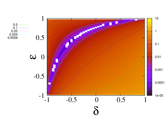
Figure 2: Histogram of $S_{tot}$ for different values of $\delta$ and $\mathcal{E}$ at $T_{h}$  =  1.0, $T_{c}=0.5$ , $E_{1}$  =  0.5, $\tau=0.4$.

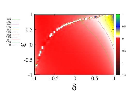
Figure 3: Histogram of $R_{err}$ for different values of $\delta$ and $\mathcal{E}$ at $T_{h}$  =  1.0, $T_{c}=0.5$, $E_{1}$ =0.5, $\tau=0.4$.

In numerical simulation we have set $T_{h}=1.0$, $T_{c}=0.5$ and $E_{1}=0.5$. We have also set Boltzmann constant $k_{B}=1$ and the interaction time of the each bit with the demon $\tau=0.4$. In fig.2 we have plotted total entropy production $S_{tot}$ for different parameter set $\delta$ and $\mathcal{E}$. We have found that it remain always positive. Hence, it proves the second law. Moreover the figure clearly indicates the reversible region, where $S_{tot}\rightarrow 0$, by simply connecting the white dots.

The relative error $R_{err}$ between the the apparent entropy production $S_{app}=S_{B}+\Delta S$ and $S_{tot}$ is defined as

$$R_{err}=\frac{S_{app}-S_{tot}}{S_{tot}}.$$ (37)

When the joint system behaves reversibly entropy production is zero and $R_{err}$ becomes undefined. The imaginary line connecting white dots in the fig.3 denotes where these phenomena is occurring. Form the figure we have found that for quite large region $R_{err}$ can take value greater than $10\%$ even it can exceed $50\%$ in certain region ($\delta\sim 1$ and high $\mathcal{E}$). Hence we can not neglect $S_{cor}$ term and $S_{tot}$ represents the proper bound.

6 Conclusions

In summary we have studied an autonomous Information engine model connecting with multiple baths, work source and information reservoir. This is the most general scenario and second law has been obtained consequently. First we have derived the second law for each individual cycle. Then we sum those inequalities to get the net inequality. The derivation is done taking into account the exact mechanism how an autonomous information machine evolves connecting to the information reservoir. We have found that this inequality is tighter compared to the earlier results [12, 13, 11, 17, 18] which only includes configuration entropy change of the tape between its output and input sequences. Besides there is a significant differences between our result with [19, 20] where second law has been derived ignoring the detailed operation. Moreover we have shown several examples where this law can be applicable. Finally from numerical simulation, we found that the correction term which depends on the correlation between output tape and final state of the demon in each cycle, is quite significant compared with the total entropy production and hence it should not be neglected.

Acknowledgements

SR thanks A M Jayannavar for broad discussions throughout the work. SR also thanks Deepak Dhar for useful discussions. SR thanks Department of Science and Technology (DST), India for the financial support through SERB NPDF.

References

- [1] Jarzynski C, equality for free energy differences, 1997 Phys. Rev. Lett. 78, 2690.
- [2] Crooks G E, Nonequilibrium measurements of free energy differences for microscopically reversible markovian systems, 1998 J. Stat. Phys. 90 1481.
- [3] Saifert U, Stochastic thermodynamics, fluctuation theorems and molecular machines, 2012 Rep. Prog. Phys. 75, 126001.
- [4] Maxwell J C, Theory of Heat, 1871 Longmans, London.
- [5] Szilard L, On the Decrease of Entropy in a Thermodynamic System by the Intervention of Intelligent Beings, 1929 Z. Phys. 53, 840.
- [6] Landauer R, Irreversibility and Heat Generation in the Computing Process, 1961, IBM J. Res. Dev. 5, 183.
- [7] Bennett C H, The thermodynamics of computation - a review, 1982 Int. J. Theor. Phys. 21, 905.
- [8] Zurek W H, Thermodynamic cost of computation, algorithmic complexity and the information metric, 1989 Nature 341, 119.
- [9] Leff H S and Rex A F, Maxwell’s Demon 2: Entropy, Classical and Quantum Information, Computing, 2003 Institute of Physics Publishing, Bristol.
- [10] Maruyama K, Nori F, and Vedral V, Colloquium: The physics of Maxwell’s demon and information, 2009 Rev. Mod. Phys. 81, 1.
- [11] Mandal D and Jarzynski C, Work and information processing in a solvable model of Maxwell’s demon, 2012 Proceedings of the National Academy of Sciences, 109, 11641.
- [12] Barato A C and Seifert U, An autonomous and reversible Maxwell’s demon, 2013 Europhys. Lett. 101, 60001.
- [13] Barato A C and Seifert U, Unifying three perspectives on information processing in stochastic thermodynamics, 2014 Phys. Rev. Lett. 112, 090601.
- [14] Deffner S and Jarzynski C, Information processing and the second law of thermodynamics: an inclusive, Hamiltonian approach, 2013 Phys Rev X 3, 041003.
- [15] Sagawa T, Ueda M, Minimal energy cost for thermodynamic information processing: measurement and information erasure, 2009 Phys. Rev. Lett. 102, 250602.
- [16] Parrondo J M R, Horowitz J M and Sagawa T, Thermodynamics of information, 2015 Nature Physics 11, 131.
- [17] Mandal D, Quan H T and Jarzynski C , Maxwell’s refrigerator: An exactly solvable model, 2013 Phys. Rev. Lett. 111, 030602.
- [18] Rana S, Jayannavar A. M., A multipurpose information engine that can go beyond the Carnot limit, 2016, J. Stat Mech: Theo. and Exp, 10, 103207.
- [19] Boyd A B, Mandal D, Crutchfield J P, Identifying functional thermodynamics in autonomous Maxwellian ratchets, 2016 New Journal of Physics 18, 023049.
- [20] Boyd A B, Mandal D, Crutchfield J P, Correlation-powered information engines and the thermodynamics of self-correction, 2017 Phys. Rev. E 95, 012152.
- [21] Merhav N, Sequence complexity and work extraction, 2015 J. Stat Mech: Theo. and Exp. 06, 06037.
- [22] Merhav N, Relation between work and entropy production for general information driven finite state engines, 2017 Journal of Statistical Mechanics: Theory and Experiment 2, 023207.
- [23] N. G. van Kampen,Stochastic Processes in Physics and Chemistry, (Elsevier, Amsterdam, 2007), Chap V, ed.
- [24] T. M. Cover and J. A. Thomas, Elements of Information Theory(Wiley-Interscience, Hoboken, New Jersey, 2006).