The Ring Produced by an Extra-Galactic Superbubble in Flat Cosmology

Abstract

A superbubble which advances in a symmetric Navarro–Frenk–White density profile or in an auto-gravitating density profile generates a thick shell with a radius that can reach 10 kpc. The application of the symmetric and asymmetric image theory to this thick 3D shell produces a ring in the 2D map of intensity and a characteristic ‘U’ shape in the case of 1D cut of the intensity. A comparison of such a ring originating from a superbubble is made with the Einstein’s ring. A Taylor approximation of order 10 for the angular diameter distance is derived in order to deal with high values of the redshift.

Keywords: Cosmology; Observational cosmology; Gravitational lenses and luminous arcs

1 Introduction

A first theoretical prediction of the existence of gravitational lenses (GL) is due to Einstein [1] where the formulae for the optical properties of a gravitational lens for star A and B were derived. A first sketch which dates back to 1912 is reported at p.585 in [2]. The historical context of the GL is outlined in [3] and ONLINE information can be found at http://www.einstein-online.info/. After 43 years a first GL was observed in the form of a close pair of blue stellar objects of magnitude 17 with a separation of 5.7 arc sec at redshift 1.405, 0957 + 561 A, B, see [4]. This double system is also known as the ”Twin Quasar” and a Figure which reports a 2014 image of the Hubble Space Telescope (HST) for objects A and B is available at https://www.nasa.gov/content/goddard/hubble-hubble-seeing-double/.

At the moment of writing, the GL is used routinely as an explanation for lensed objects, see the following reviews [5, 6, 7, 8]. As an example of current observations, 28 gravitationally lensed quasars have been observed by the Subaru Telescope, see [9], where for each system a mass model was derived. Another example is given by the SDSS-III Baryon Oscillation Spectroscopic Survey (BOSS), see [10], where 13 two-image quasar lenses have been observed and the relative Einstein’s radius reported in arcsec. A first classification separates the strong lensing, such as an Einstein ring (ER) and the arcs from the weak lensing, such as the shape deformation of background galaxies.

The strong lensing is verified when the light from a distant background source, such as a galaxy or quasar, is deflected into multiple paths by an intervening galaxy or a cluster of galaxies producing multiple images of the background source: examples are the ER and the multiple arcs in cluster of galaxies, see https://apod.nasa.gov/apod/ap160828.html.

In the case of weak lensing the lens is not strong enough to form multiple images or arcs, but the source can be distorted: both stretched (shear) and magnified (convergence), see [11] and [12]. The first cluster of galaxies observed with the weak lensing effect is reported by [13].

We now introduce supershells, which were unknown when the GL was postulated. Supershells started to be observed firstly in our galaxy by [14], where 17 expanding H I shells were classified, and secondly in external galaxies, see as an example [15], where many supershells were observed in NGC 1569. In order to model such complex objects, the term super bubble (SB) has been introduced but unfortunately the astronomers often associate the SBs with sizes of $\approx$ 10–100 pc and the supershells with ring-like structures with sizes of $\approx$ 1 kpc. At the same time an application of the theory of image explains the limb-brightening visible on the maps of intensity of SBs and allows associating the observed filaments to undetectable SBs, see [16].

This paper derives, in Section 2, an approximate solution for the angular diameter distance in flat cosmology. Section 3 briefly reviews the existing knowledge of ERs. Section 4 derives an equation of motion for an SB in a Navarro–Frenk–White (NFW) density profile. Section 5 adopts a recursive equation in order to model an asymmetric motion for an SB in an auto-gravitating density profile.

Section 6.3 applies the symmetrical and the asymmetrical image theory to the advancing shell of an SB.

2 The flat cosmology

Following eq. (2.1) of [17], the luminosity distance in flat cosmology, $d_{\rm{L}}$, is

$$d_{\rm{L}}(z;c,H_{0},\Omega_{\rm M})=\frac{c}{H_{0}}(1+z)\int_{\frac{1}{1+z}}^{1}\frac{da}{\sqrt{\Omega_{\rm M}a+(1-\Omega_{\rm M})a^{4}}}\quad,$$ (1)

where $H_{0}$ is the Hubble constant expressed in $\mathrm{km\,s^{-1}\,Mpc^{-1}}$, $c$ is the velocity of light expressed in $\mathrm{km\,s^{-1}}$, $z$ is the redshift, $a$ is the scale factor, and $\Omega_{\rm M}$ is

$$\Omega_{\rm M}=\frac{8\pi\,G\,\rho_{0}}{3\,H_{0}^{2}}\quad,$$ (2)

where $G$ is the Newtonian gravitational constant and $\rho_{0}$ is the mass density at the present time. An analytical solution for the luminosity distance exists in the complex plane, see [18]. Here we deal with an approximate solution for the luminosity distance in the framework of a flat universe adopting the same cosmological parameters of [19] which are $H_{0}=72\,\mathrm{km\,s^{-1}\,Mpc^{-1}}$, $\Omega_{\rm M}=0.26$ and $\Omega_{\Lambda}=0.74$. An approximate solution for the luminosity distance, $d_{\rm{L,10}}(z)$, is given by a Taylor expansion of order 10 about $a=1$ for the argument of the integral (1)

$$d_{\rm{L,10}}(z)=4163.78\,\left(1+z\right)\Bigg{(}2.75+0.12882\,\left(1+z\right)^{-10}$$

$$-1.34123\,\left(1+z\right)^{-9}+6.23877\,\left(1+z\right)^{-8}-17.0003\,\left(1+z\right)^{-7}$$

$$+29.8761\,\left(1+z\right)^{-6}-35.1727\,\left(1+z\right)^{-5}+28.2558\,\left(1+z\right)^{-4}$$

$$-16.5327\,\left(1+z\right)^{-3}+9.26107\,\left(1+z\right)^{-2}-6.46\,\left(1+z\right)^{-1}\Bigg{)}\quad.$$ (3)

More details on the analytical solution for the luminosity distance in the case of flat cosmology can be found in [20] and Figure 1 reports the comparison between the above analytical solution, and Taylor expansion of order 10, 8 and 2.

Figure 1: The analytical solution (red line ) for the luminosity distance and three Taylor approximated solutions with color coding as in the legend.

The goodness of the Taylor approximation is evaluated through the percentage error, $\delta$, which is

$$\delta=\frac{\big{|}d_{\rm{L}}(z)-d_{\rm{L,10}}(z)_{10}\big{|}}{d_{\rm{L}}(z)}\times 100\quad.$$ (4)

As an example, Table 1 reports the percentage error at z= 4 for three order of expansion; is clear the progressive decrease of the percentage error with the increase in the order of expansion.

Table 1: Percentage error between analytical solution and approximated Taylor solution of a given order at z=4.

Taylor  order	$\delta$
2	22.6 %
8	2.2 %
10	0.61 %

Another useful distance is the angular diameter distance, $d_{\rm{A}}$, which is

$$d_{\rm{A}}=\frac{d_{\rm{L}}}{(1+z)^{2}}\quad,$$ (5)

see [21] and the Taylor approximation for the angular diameter distance, $d_{\rm{A,10}}$

$$d_{\rm{A,10}}=\frac{d_{\rm{L,10}}}{(1+z)^{2}}\quad.$$ (6)

As a practical example of the above equation, the angular scale of $1\,arcsec$ is $7.73$ kpc at $z=3.042$ when [19] quotes $7.78$ kpc: this means a percentage error of 0.63% between the two values. Another check can be done with the Ned Wright’s Cosmology Calculator [22] available at http://www.astro.ucla.edu/~wright/CosmoCalc.html: it quotes a scale of 7.775 $kpc\,arcsec^{-1}$ which means a percentage error of 0.57% with respect to our value. In this section we have derived the cosmological scaling that allows to fix the dimension of the ER.

3 The ER

This section reviews the simplest version of the ER and reports the observations of two recent ERs.

3.1 The theory

In the case of a circularly symmetric lens and when the source and the length are on the same line of sight, the ER radius in radiant is

$$\theta_{E}=\sqrt{\frac{4GM(\theta_{E})}{c^{2}}\frac{D_{ds}}{D_{d}\,D_{s}}}\quad,$$ (7)

where $M(\theta_{E})$ is the mass enclosed inside the ER radius, $D_{d,s,ds}$ are the lens, source and lens–source distances, respectively, $G$ is the Newtonian gravitational constant, and $c$ is the velocity of light, see eq. (20) in [23] and eq. (1) in [24]. The mass of the ER can be expressed in units of solar mass, $M_{\hbox{$\odot$}}$:

$$M(\theta_{E,arcsec})=1.228\,10^{8}\,{\frac{{\Theta_{{{\it E,arcsec}}}}^{2}D_{{{\it ds},{\mathrm{Mpc}}}}D_{{s,{\mathrm{Mpc}}}}}{D_{{d,{\mathrm{Mpc}}}}}}\,M_{\hbox{$\odot$}}\quad,$$ (8)

where $\theta_{E,arcsec}$ is the ER radius in ${arcsec}$ and the three distances are expressed in Mpc.

3.2 The galaxy–galaxy lensing system SDP.81

The ring associated with the galaxy SDP.81, see [25], is generally explained by a GL. In this framework we have a foreground galaxy at $z=0.2999$ and a background galaxy at $z=0.3042$. This ring has been studied with the Atacama Large Millimeter/sub-millimeter Array (ALMA) by [19, 26, 27, 28, 29, 30]. The system SDP.81 as analysed by ALMA presents 14 molecular clumps along the two main lensed arcs. We can therefore speak of the ring appearance as a ‘grand design’ and we now test the circular hypothesis. In order to test the departure from a circle, an observational percentage of reliability is introduced that uses both the size and the shape,

$$\epsilon_{\mathrm{obs}}=100(1-\frac{\sum_{j}|R_{\mathrm{obs}}-R_{\mathrm{ave}}|_{j}}{\sum_{j}{R_{\mathrm{obs}}}_{j}})\quad,$$ (9)

where $R_{\mathrm{obs}}$ is the observed radius in $arcsec$ and $R_{\mathrm{ave}}$ is the averaged radius in $arcsec$ which is $R_{\mathrm{ave}}=1.54\,arcsec$. Figure 2 reports the astronomical data of SDP.81 and the percentage of reliability is $\epsilon_{\mathrm{obs}}=92.78\%$.

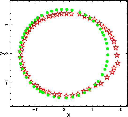
Figure 2: Real data of SDP.81 ring (empty red stars) and averaged circle (full green points). The real data are extracted by the author from Figure 6 in [30] using WebPlotDigitizer.

3.3 Canarias ER

The object IAC J010127-334319 has been detected in the optical region with the Gran Telescopio CANARIAS; the radius of the ER is $\theta_{E}=2.16\,{arcsec}$, see [24]. As an example, inserting the above radius, $D_{{s,{\mathrm{Mpc}}}}=1192$ Mpc, $D_{{ls,{\mathrm{Mpc}}}}=498$ Mpc and $D_{{l,{\mathrm{Mpc}}}}=951$ Mpc in Eq. (8), we obtain a mass for the foreground galaxy of $M(\theta_{E,arcsec})=1.3\,10^{12}M_{\hbox{$\odot$}}$.

4 The equation of motion of a symmetrical SB

The density is assumed to have a Navarro–Frenk–White (NFW ) dependence on $r$ in spherical coordinates:

$$\rho(r;r_{0},b,\rho_{0})=\frac{\rho_{{0}}r_{{0}}\left(b+r_{{0}}\right)^{2}}{r\left(b+r\right)^{2}}\quad,$$ (10)

where $b$ represents the scale, see [31] for more details. The piece-wise density is

$$\rho(r;r_{0},b,\rho_{0})=\left\{\begin{array}[]{ll}\rho_{0}&\mbox{if $r\leq r_{0}$ }\\ \frac{\rho_{{0}}r_{{0}}\left(b+r_{{0}}\right)^{2}}{r\left(b+r\right)^{2}}&\mbox{if $r>r_{0}$ }\end{array}\right.$$ (11)

The total mass swept, $M(r;r_{0},b,\rho_{0})$, in the interval $[0,r]$ is

$$M(r;r_{0},b,\rho_{0})=\frac{1}{3\,b+3\,r}\Bigg{(}-4\,r_{{0}}\pi\,\rho_{{0}}\Big{(}3\,\ln(b+r_{{0}}){b}^{3}+3\,\ln(b+r_{{0}}){b}^{2}r$$

$$+6\,\ln(b+r_{{0}}){b}^{2}r_{{0}}+6\,\ln(b+r_{{0}})brr_{{0}}+3\,\ln(b+r_{{0}})b{r_{{0}}}^{2}+3\,\ln(b+r_{{0}})r{r_{{0}}}^{2}$$

$$-3\,\ln(b+r){b}^{3}-3\,\ln(b+r){b}^{2}r-6\,\ln(b+r){b}^{2}r_{{0}}-6\,\ln(b+r)brr_{{0}}$$

$$-3\,\ln(b+r)b{r_{{0}}}^{2}-3\,\ln(b+r)r{r_{{0}}}^{2}+3\,{b}^{2}r-3\,{b}^{2}r_{{0}}+3\,br_{{0}}r$$

$$-4\,b{r_{{0}}}^{2}-{r_{{0}}}^{2}r\Big{)}\Bigg{)}\quad.$$ (12)

The conservation of momentum in spherical coordinates in the framework of the thin layer approximation states that

$$M_{0}(r_{0})\,v_{0}=M(r)\,v\quad,$$ (13)

where $M_{0}(r_{0})$ and $M(r)$ are the swept masses at $r_{0}$ and $r$, and $v_{0}$ and $v$ are the velocities of the thin layer at $r_{0}$ and $r$. The velocity is, therefore,

$$\frac{dr}{dt}=\frac{NE}{DE}\quad,$$ (14)

where

$$NE=-{r_{{0}}}^{2}v_{{0}}\left(b+r\right)\quad,$$

and

$$DE=3\,\ln(b+r_{{0}}){b}^{3}+3\,\ln(b+r_{{0}}){b}^{2}r+6\,\ln(b+r_{{0}}){b}^{2}r_{{0}}$$

$$+6\,\ln(b+r_{{0}})brr_{{0}}+3\,\ln(b+r_{{0}})b{r_{{0}}}^{2}+3\,\ln(b+r_{{0}})r{r_{{0}}}^{2}-3\,\ln(b+r){b}^{3}$$

$$-3\,\ln(b+r){b}^{2}r-6\,\ln(b+r){b}^{2}r_{{0}}-6\,\ln(b+r)brr_{{0}}-3\,\ln(b+r)b{r_{{0}}}^{2}$$

$$-3\,\ln(b+r)r{r_{{0}}}^{2}+3\,{b}^{2}r-3\,{b}^{2}r_{{0}}+3\,br_{{0}}r-4\,b{r_{{0}}}^{2}-{r_{{0}}}^{2}r\quad.$$

The integration of the above differential equation of the first order gives the following non-linear equation:

$$\frac{1}{{r_{{0}}}^{2}v_{{0}}}\Bigg{(}-6\,(b+r_{{0}})^{2}(b+r/2)\ln(b+r_{{0}})+6\,(b+r_{{0}})^{2}(b+r/2)\ln(b+r)$$

$$-6\,(r-r_{{0}})({b}^{2}+3/2\,br_{{0}}+1/3\,{r_{{0}}}^{2})\Bigg{)}=\left(t-{\it t_{0}}\right)$$ (15)

The above non-linear equation does not have an analytical solution for the radius, $r$, as a function of time. The astrophysical units are pc for length and yr for time. With these units, the initial velocity is $v_{0}$(km s${}^{-1})=9.7968\,10^{5}v_{0}$(pc yr${}^{-1})$. The energy conserving phase of an SB in the presence of constant density allows setting up the initial conditions, and the radius is

$$R=111.552\,{\frac{\sqrt[5]{{\it N^{*}}}\sqrt[5]{E_{{51}}}{t_{{7}}}^{3/5}}{\sqrt[5]{n_{0}}}}\quad{\mathrm{pc}}\quad,$$ (16)

where $t_{7}$ is the time expressed in units of $10^{7}$ yr, $E_{51}$ is the energy expressed in units of $10^{51}$ erg, $n_{0}$ is the number density expressed in particles $\mathrm{cm}^{-3}$ (density $\rho_{0}=n_{0}m$, where $m=1.4m_{\mathrm{H}}$) and $N^{*}$ is the number of SN explosions in $5.0\cdot 10^{7}$ yr and therefore is a rate, see see eq. (10.38) in [32]. The velocity of an SB in such a phase is

$$v_{0}=0.416324\,{\frac{{5}^{2/5}{14}^{4/5}\sqrt[5]{{\it N^{*}}}\sqrt[5]{E_{{51}}}}{\sqrt[5]{n_{0}}{t_{{7}}}^{2/5}}}\quad\frac{km}{s}\quad.$$ (17)

The initial condition for $r_{0}$ and $v_{0}$ are now fixed by the energy conserving phase for an SB evolving in a medium at constant density. The free parameters of the model are reported in Table 2, Figure 3 reports the law of motion and Figure 4 the behaviour of the velocity as a function of time.

Table 2: Theoretical parameters of an SB evolving in a medium with a NFW profile.

Name	$t_{0}$(yr)	$E_{51}$	$n_{0}\,(\frac{1}{{\mathrm{cm}}^{3}})$	b(pc)	$N^{*}$
SDP.81	10000	1	$10^{-4}$	1	1000

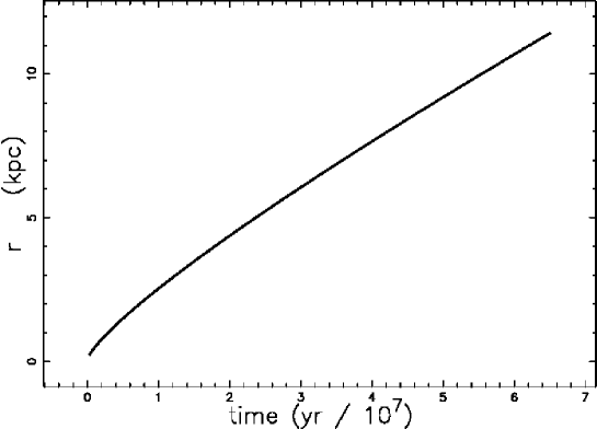
Figure 3: Numerical solution for the radius as a function of time for SB associated with SDP.81 (full line), parameters as in Table 2.

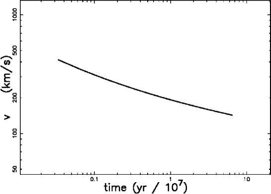
Figure 4: Velocity as a function of time for SDP.81 (full line), parameters as in Table 2, both axes are logarithmic.

Once we have fixed the standard radius of SDP.81 at $r=11.39$ kpc, we evaluate the pair of values for $b$ (the scale) and for $t$ (the time) that allows such a value of the radius, see Figure 5.

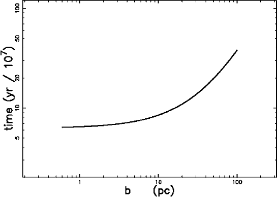
Figure 5: The relation between $b$ and time which produces $r=11.39$ kpc, other parameters as in Table 2. Both axes are logarithmic.

The pair of values of $n_{0}$ (initial number density) and $t$ (the time) which produces the standard value of the radius is reported in Figure 6; Figure 7 conversely reports the actual velocity of the SB associated with SDP.81 as function of $n_{0}$.

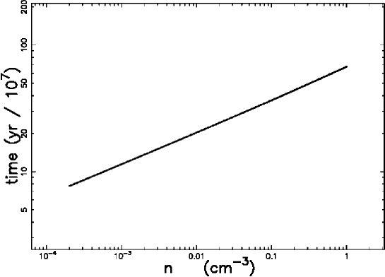
Figure 6: The relation between $n_{0}$ and the time which produces $r=11.39$ kpc, other parameters as in Table 2. Both axes are logarithmic.

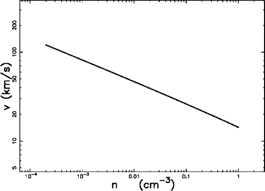
Figure 7: The actual velocity as a function of $n_{0}$ when the standard radius is $r=11.39$ kpc, other parameters as in Table 2. Both axes are logarithmic.

The swept mass can be expressed in the number of solar masses, $M_{\hbox{$\odot$}}$, and, with parameters as in Table 2, is

$$M=3732.709\,n_{0}\,M_{\hbox{$\odot$}}\quad.$$ (18)

5 The equation of motion of an asymmetrical SB

In order to simulate an asymmetric SB we briefly review a numerical algorithm developed in [16]. We assume a number density distribution as

$$n(z)=n_{0}sech^{2}(\frac{z}{2\,h})\quad,$$ (19)

where $n_{0}$ is the density at $z=0$, $h$ is a scaling parameter, and $sech$ is the hyperbolic secant ([33, 34, 35, 36]).

We now analyze the case of an expansion that starts from a given galactic height $z$, denoted by $z_{\mathrm{OB}}$, which represents the OB associations. It is not possible to find $r$ analytically and a numerical method should be implemented.

The following two recursive equations are found when momentum conservation is applied:

$$r_{n+1}=r_{n}+v_{n}\Delta t$$

$$v_{n+1}=v_{n}\Bigl{(}\frac{M_{n}(r_{n})}{M_{n+1}(r_{n+1})}\Bigr{)}\quad,$$ (20)

where $r_{n}$, $v_{n}$, $M_{n}$ are the temporary radius, the velocity, and the total mass, respectively, $\Delta t$ is the time step, and $n$ is the index. The advancing expansion is computed in a 3D Cartesian coordinate system ($x,y,z$) with the center of the explosion at (0,0,0). The explosion is better visualized in a 3D Cartesian coordinate system ($X,Y,Z$) in which the galactic plane is given by $Z=0$. The following translation, $T_{\mathrm{OB}}$, relates the two Cartesian coordinate systems.

$$T_{\mathrm{OB}}~{}\left\{\begin{array}[]{l}X=x\\ \vskip 6.0pt plus 2.0pt minus 2.0pt\cr Y=y\\ \vskip 6.0pt plus 2.0pt minus 2.0pt\cr Z=z+z_{\mathrm{OB}}\end{array}\right.\quad,$$ (21)

where $z_{\mathrm{OB}}$ is the distance in parsec of the OB associations from the galactic plane.

The physical units for the asymmetrical SB have not yet been specified: parsecs for length and $10^{7}\,yr$ for time are perhaps an acceptable astrophysical choice. With these units, the initial velocity $v_{{0}}=\dot{r_{0}}$ is expressed in units of pc/($10^{7}$ yr) and should be converted into km/s; this means that $v_{{0}}=10.207v_{{1}}$ where $v_{{1}}$ is the initial velocity expressed in km/s.

We are now ready to present the numerical evolution of the SB associated with SDP.81 when $z_{\mathrm{OB}}=100\mbox{pc}$, see Fig. 8.

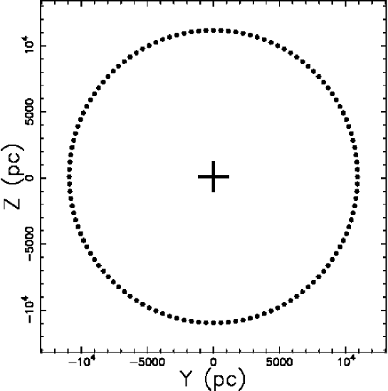
Figure 8: Section of the SB associated with SDP.81 in the Y-Z;X=0 plane when the explosion starts at $z_{\mathrm{OB}}=100\mbox{pc}$. The code parameters for the numerical couple (20) are $h=14000$ $pc$, $t_{7}=350~{}$, $t_{7,0}$ = 0.35, $r_{0}$ = 1325, $v_{0}=222\mathrm{km}\,\mathrm{s}^{-1}$, $N_{SN}$ = 140000 and $N^{*}$=2000000. The explosion site is represented by a cross.

The degree of asymmetry can be evaluated introducing the radius along the polar direction up, $r_{up}$, the polar direction down, $r_{up}$ and the equatorial direction , $r_{eq}$. In our model all the already defined three radii are different, see Table 3.

Table 3: Radii concerning SB associated with SDP.81, parameters as in Figure 8.

$$\begin{array}[]{cc}\hline\cr\vskip 3.0pt plus 1.0pt minus 1.0pt\cr\mathrm{Direction}&r(\mathrm{pc})\\ \vskip 3.0pt plus 1.0pt minus 1.0pt\cr\hline\cr\vskip 3.0pt plus 1.0pt minus 1.0pt\cr\mathrm{Equatorial}&10906\\ \mathrm{Polar~{}up}&11077\\ \mathrm{Polar~{}down}&11068\\ \vskip 3.0pt plus 1.0pt minus 1.0pt\cr\hline\cr\end{array}$$

We can evaluate the radius and the velocity as function of the direction plotting the radius and the direction in section in the Y-Z;X=0 plane, see Figures 9 and 10.

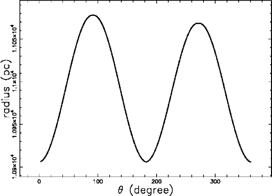
Figure 9: Radius in $pc$ of the SB associated with SDP.81 as a function of the position angle in degrees for a self-gravitating medium, parameters as in Figure 8.

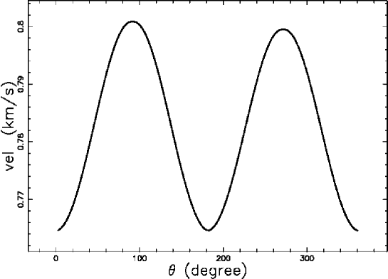
Figure 10: Velocity in $\frac{km}{s}$ of the the SB associated with SDP.81 as a function of the position angle in degrees for a self-gravitating medium, parameters as in Figure 8.

6 The image

We now briefly review the basic equations of the radiative transfer equation, the conversion of the flux of energy into luminosity, the symmetric and the asymmetric theory of the image.

6.1 Radiative transfer equation

The transfer equation in the presence of emission and absorption, see for example eqn.(1.23) in [37] or eqn.(9.4) in [38] or eqn.(2.27) in [39], is

$$\frac{dI_{\nu}}{ds}=-k_{\nu}\zeta I_{\nu}+j_{\nu}\zeta\quad,$$ (22)

where $I_{\nu}$ is the specific intensity or spectral brightness, $s$ is the line of sight, $j_{\nu}$ the emission coefficient, $k_{\nu}$ a mass absorption coefficient, $\zeta$ the mass density at position $s$, and the index $\nu$ denotes the involved frequency of emission. The solution to Eq. (22) is

$$I_{\nu}(\tau_{\nu})=\frac{j_{\nu}}{k_{\nu}}(1-e^{-\tau_{\nu}(s)})\quad,$$ (23)

where $\tau_{\nu}$ is the optical depth at frequency $\nu$

$$d\tau_{\nu}=k_{\nu}\zeta ds\quad.$$ (24)

We now continue analysing the case of an optically thin layer in which $\tau_{\nu}$ is very small (or $k_{\nu}$ very small) and the density $\zeta$ is replaced by the number density of particles, $n(s)$. In the following, the emissivity is taken to be proportional to the number density

$$j_{\nu}\zeta=Kn(s)\quad,$$ (25)

where $K$ is a constant. The intensity is therefore

$$I_{\nu}(s)=I_{0}+K\int_{s_{0}}^{s}n(s\prime)ds\prime,$$ (26)

where $I_{0}$ is the intensity at the point $s_{0}$. The MKS units of the intensity are W m^-2 Hz${{}^{-}1}$  sr^-1. The increase in brightness is proportional to the number density integrated along the line of sight: in the case of constant number density, it is proportional only to the line of sight.

As an example, synchrotron emission has an intensity proportional to $l$, the dimension of the radiating region, in the case of a constant number density of the radiating particles, see formula (1.175) of [40].

6.2 The source of luminosity

The ultimate source of the observed luminosity is assumed to be the rate of kinetic energy, $L_{m}$,

$$L_{m}=\frac{1}{2}\rho AV^{3}\quad,$$ (27)

where $A$ is the considered area, $V$ is the velocity of a spherical SB and $\rho$ is the density in the advancing layer of a spherical SB. In the case of the spherical expansion of an SB, $A=4\pi r^{2}$, where $r$ is the instantaneous radius of the SB, which means

$$L_{m}=\frac{1}{2}\rho 4\pi r^{2}V^{3}\quad.$$ (28)

The units of the luminosity are W in MKS and erg s^-1 in CGS. The astrophysical version of the the rate of kinetic energy, $L_{ma}$, is

$$L_{ma}={1.39\times 10^{29}}\,{\it n_{1}}\,{{\it r_{1}}}^{2}{{\it v_{1}}}^{3}\frac{{\mathrm{ergs}}}{{\mathrm{s}}}\quad,$$ (29)

where $n_{1}$ is the number density expressed in units of $1~{}\frac{{\mathrm{particle}}}{{\mathrm{cm}}^{3}}$, $r_{1}$ is the radius in parsecs, and $v_{1}$ is the velocity in km/s. As an example, according to Figure 7, inserting $r_{1}=11.39\,10^{3}$, $n_{1}=0.1$ and $v_{1}$ =26.08 in the above formula, the maximum available mechanical luminosity is $L_{ma}=3.2\,10^{40}\,\frac{{\mathrm{ergs}}}{{\mathrm{s}}}$. The spectral luminosity, $L_{\nu}$, at a given frequency $\nu$ is

$$L_{\nu}=4\pi d_{\rm{L}}^{2}S_{\nu}\quad,$$ (30)

where $S_{\nu}$ is the observed flux density at a given frequency $\nu$ with MKS units as W m^-2 Hz^-1. The observed luminosity at a given frequency $\nu$ can be expressed as

$$L_{\nu}=\epsilon L_{ma}\quad,$$ (31)

where $\epsilon$ is a conversion constant from the mechanical luminosity to the observed luminosity. More details on the synchrotron luminosity and the connected astrophysical units can be found in [39].

6.3 The symmetrical image theory

We assume that the number density of the emitting matter $n$ is variable, and in particular rises from 0 at $r=a$ to a maximum value $n_{m}$, remains constant up to $r=b$, and then falls again to 0. This geometrical description is shown in Figure 11.

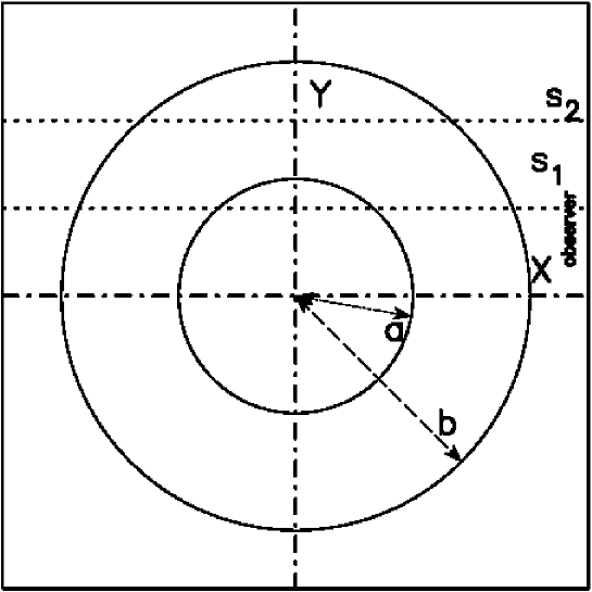
Figure 11: The two circles (sections of spheres) which include the region with constant number density of emitting matter are represented by a full line. The observer is situated along the $x$ direction, and three lines of sight are indicated.

The length of the line of sight, when the observer is situated at the infinity of the $x$-axis, is the locus parallel to the $x$-axis which crosses the position $y$ in a Cartesian $x-y$ plane and terminates at the external circle of radius $b$. The locus length is

$$l_{0a}=2\times(\sqrt{b^{2}-y^{2}}-\sqrt{a^{2}-y^{2}})\quad;0\leq y<a$$

$$l_{ab}=2\times(\sqrt{b^{2}-y^{2}})\quad;a\leq y<b\quad.$$ (32)

When the number density of the emitting matter $n_{m}$ is constant between two spheres of radii $a$ and $b$, the intensity of radiation is

$$I_{0a}=K_{I}\times n_{m}\times 2\times(\sqrt{b^{2}-y^{2}}-\sqrt{a^{2}-y^{2}})\quad;0\leq y<a$$

$$I_{ab}=K_{I}\times n_{m}\times 2\times(\sqrt{b^{2}-y^{2}})\quad;a\leq y<b\quad,$$ (33)

where $K_{I}$ is a constant. The ratio between the theoretical intensity at the maximum $(y=a)$ and at the minimum ($y=0$) is given by

$$\frac{I(y=a)}{I(y=0)}=\frac{\sqrt{b^{2}-a^{2}}}{b-a}\quad.$$ (34)

The parameter $b$ is identified with the external radius, which means the advancing radius of an SB. The parameter $a$ can be found from the following formula:

$$a=\frac{b\left((\frac{I(y=a)}{I(y=0)})_{obs}^{2}-1\right)}{\left((\frac{I(y=a)}{I(y=0)})_{obs}^{2}+1\right)}\quad,$$ (35)

where $(\frac{I(y=a)}{I(y=0)})_{obs}$ is the observed ratio between the maximum intensity at the rim and the intensity at the center. The distance $\Delta y$ after which the intensity is decreased of a factor $f$ in the region $a\leq y<b$ is

$$\Delta y=\frac{2\sqrt{{b}^{2}{f}^{2}+{a}^{2}-{b}^{2}}-\sqrt{{a}^{2}{f}^{4}-{b}^{2}{f}^{4}+2{a}^{2}{f}^{2}+2{b}^{2}{f}^{2}+{a}^{2}-{b}^{2}}}{2\,f}\quad.$$ (36)

We can now evaluate the half-width half-maximum by analogy with the Gaussian profile $HWHM_{U}$, which is obtained by the previous formula upon inserting $f=2$:

$$HWHM_{U}=\frac{1}{2}\,\sqrt{{a}^{2}+3\,{b}^{2}}-\frac{1}{4}\,\sqrt{25\,{a}^{2}-9\,{b}^{2}}\quad.$$ (37)

In the above model, $b$ is associated with the radius of the outer region of the observed ring, $a$ conversely can be deduced from the observed $HWHM_{U}$:

$$a=$$

$$\frac{1}{21}\,\sqrt{441\,{b}^{2}+464\,{{\it HWHM_{U}}}^{2}-32\,\sqrt{441\,{b}^{2}{{\it HWHM_{U}}}^{2}+100\,{{\it HWHM_{U}}}^{4}}}\quad.$$ (38)

As an example, inserting in the above formula $b=1.54\,arcsec$ and $HWHM_{U}=0.1\,arcsec$, we obtain $a=1.46\,arcsec$. A cut in the theoretical intensity of SDP.81, see Section 3.2, is reported in Figure 12 and a theoretical image in Figure 13.

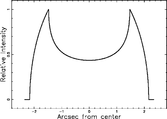
Figure 12: Cut of the intensity ${\it I}$ of the ring model, Equation (33), crossing the center. The $x$ and $y$ axes are in $arcsec$, $a=1.23\,arcsec$, $b=1.54\,arcsec$ and $\frac{I(y=a)}{I(y=0)}=3$. This cut refers to SDP.81.

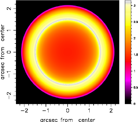
Figure 13: Contour map of ${\it I}$, the $x$ and $y$ axes are in $arcsec$, parameters as in Figure 12.

The effect of the insertion of a threshold intensity, $I_{tr}$, which is connected with the observational techniques, is now analysed. The threshold intensity can be parametrized to $I_{max}$, the maximum value of intensity characterizing the ring: a typical image with a hole is visible in Figure 14 when $I_{tr}=I_{max}/fac$, where $fac$ is a parameter which allows matching theory with observations.

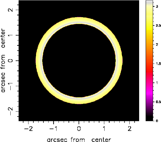
Figure 14: The same as Figure 13 but with $I_{tr}=I_{max}/fac$, parameters as in Figure 12 and $fac=1.2$.

A comparison between the theoretical intensity and the theoretical flux can be made through the formula (30) and due to the fact that $d_{\rm{L}}$ is assumed to constant over all the astrophysical image, the theoretical intensity and the theoretical flux are assumed to scale in the same way.

The theoretical flux profiles for IAC J010127-334319, see Section 3.3, is reported in Figure 15.

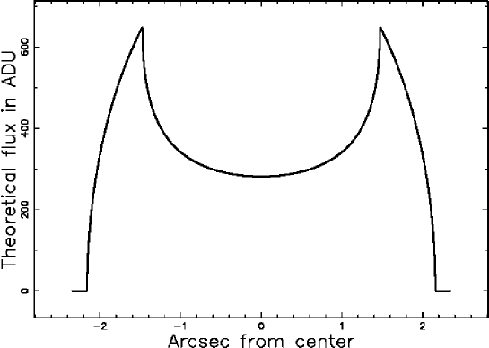
Figure 15: Theoretical flux for the Canarias ring. The $x$ and $y$ axes are in $arcsec$, $a=1.47\,arcsec$, $b=2.16\,arcsec$ and $\frac{I(y=a)}{I(y=0)}=2.30$. This cut refers to IAC J010127-334319.

The linear relation between the angular distance, in pc, and the projected distance on the sky in $arcsec$ allows to state the following

Theorem 1.

The ‘U’ profile of cut in theoretical flux for a symmetric ER is independent of the exact value of the angular distance.

6.4 The asymmetrical image theory

We now explain a numerical algorithm which allows us to build the complex image of an asymmetrical SB.

• An empty (value=0) memory grid ${\mathcal{M}}(i,j,k)$ which contains $NDIM^{3}$ pixels is considered

• We first generate an internal 3D surface by rotating the section of $180^{\circ}$ around the polar direction and a second external surface at a fixed distance $\Delta R$ from the first surface. As an example, we fixed $\Delta r$ = $0.03r_{max}$, where $r_{max}$ is the maximum radius of expansion. The points on the memory grid which lie between the internal and the external surfaces are memorized on ${\mathcal{M}}(i,j,k)$ with a variable integer number according to formula (28) and density $\rho$ proportional to the swept mass.

• Each point of ${\mathcal{M}}(i,j,k)$ has spatial coordinates $x,y,z$ which can be represented by the following $1\times 3$ matrix, $A$,

  $$A=\left[\begin{array}[]{c}x\\ \vskip 6.0pt plus 2.0pt minus 2.0pt\cr y\\ \vskip 6.0pt plus 2.0pt minus 2.0pt\cr{\it z}\end{array}\right]\quad.$$ (39)

  The orientation of the object is characterized by the Euler angles $(\Phi,\Theta,\Psi)$ and therefore by a total $3\times 3$ rotation matrix, $E$, see [41]. The matrix point is represented by the following $1\times 3$ matrix, $B$,

  $$B=E\cdot A\quad.$$ (40)

• The intensity map is obtained by summing the points of the rotated images along a particular direction.

• The effect of the insertion of a threshold intensity, $I_{tr}$, given by the observational techniques, is now analysed. The threshold intensity can be parametrized by $I_{max}$, the maximum value of intensity which characterizes the map, see [42].

An ideal image of the intensity of the Canarias ring is shown in Fig. 16.

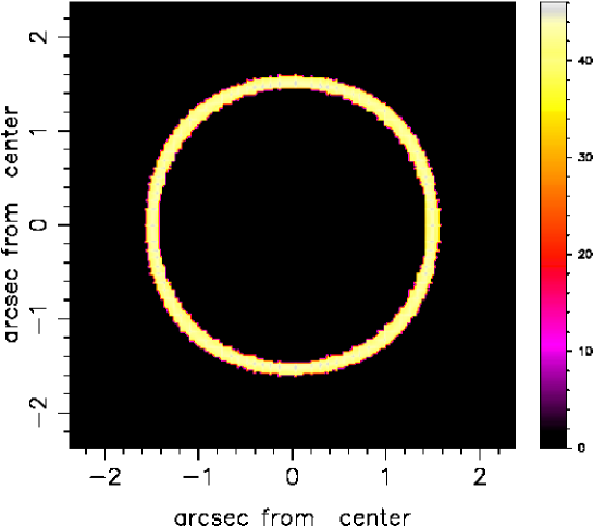
Figure 16: Map of the theoretical intensity of the Canarias ring. Physical parameters as in Fig. 8. The three Euler angles characterizing the orientation are $\Phi$=90 ^∘, $\Theta$=90 ^∘ and $\Psi$=90 ^∘. This combination of Euler angles corresponds to the rotated image with the polar axis along the z-axis. In this map $I_{tr}=I_{max}/1.2.$

The theoretical flux which is here assumed to scale as the flux of kinetic energy as represented by eqn.(28), is reported in Figure 17. The percentage of reliability which characterizes the observed and the theoretical variations in intensity of the above figure is $\epsilon_{\mathrm{obs}}=92.7\%$.

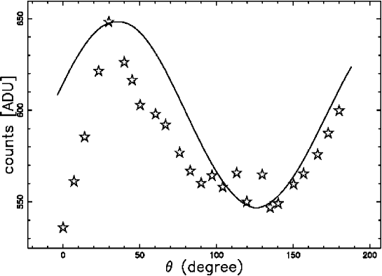
Figure 17: Theoretical counts (full line ) and observed counts (empty stars) in ADU for the SB associated with SDP.81 as a function of the position angle, parameters as in Figure 8.

7 Conclusions

Flat cosmology: In order to have a reliable evaluation of the radius of SDP.81 we have provided a Taylor approximation of order 10 for the luminosity distance in the framework of the flat cosmology. The percentage error between analytical solution and approximated solution when $z=3.04$ (the redshift of SDP.81) is $\delta=0.588\%$.

Symmetric evolution of an SB: The motion of a SB advancing in a medium with decreasing density in spherical symmetry is analyzed. The type of density profile here adopted is a NFW profile which has three free parameters, $r_{0}$ ,$b$ and $\rho_{0}$. The available astronomical data does not allow to close the equations at $r=11.39$ kpc (the radius of SDP.81). A numerical relationship which connects the number density with the lifetime of a SB is reported in Figure 6 and an approximation of the above relationship is $\frac{t}{10^{7}\,yr}=67.36n_{0}^{0.26}$ when $b=1\,pc$ and $r_{0}=44\,pc$.

Symmetric Image theory: The transfer equation for the luminous intensity in the case of optically thin layer is reduced in the case of spherical symmetry to the evaluation of a length between lower and upper radius along the line of sight, see eqn.32. The cut in intensity has a characteristic ”U” shape, see eqn.(33), which also characterizes the image of ER associated with the galaxy SDP.81.

Asymmetric Image theory:

The layer between a complex 3D advancing surface with radius, $r_{a}$, function of two angles in polar coordinates (external surface) and $r_{a}-\Delta r$ (internal surface) is filled with N random points. After a rotation characterized by three Euler angles which align the 3D layer with the observer, the image is obtained by summing a 3D visitation grid over one index, see image 16. The variations for the Canarias ER of the flux counts in ADU as function of the angle can be modeled because radius, velocity and therefore flux of kinetic energy are different for each chosen direction, see Figure 17.

REFERENCES

- [1] Einstein A 1936 Lens-Like Action of a Star by the Deviation of Light in the Gravitational Field Science 84, 506
- [2] Einstein A 1994 The Collected Papers of Albert Einstein, Volume 3: The Swiss Years: Writings, 1909-1911. (Princeton, NJ: Princeton University Press)
- [3] Valls-Gabaud D 2006 The conceptual origins of gravitational lensing in J M Alimi and A Füzfa, eds, Albert Einstein Century International Conference vol 861 of American Institute of Physics Conference Series pp 1163–1163 (Preprint 1206.1165)
- [4] Walsh D, Carswell R F and Weymann R J 1979 0957 + 561 A, B - Twin quasistellar objects or gravitational lens Nature 279, 381
- [5] Blandford R D and Narayan R 1992 Cosmological applications of gravitational lensing ARA&A 30, 311
- [6] Mellier Y 1999 Probing the Universe with Weak Lensing ARA&A 37, 127 (Preprint astro-ph/9812172)
- [7] Refregier A 2003 Weak Gravitational Lensing by Large-Scale Structure ARA&A 41, 645 (Preprint astro-ph/0307212)
- [8] Treu T 2010 Strong Lensing by Galaxies ARA&A 48, 87 (Preprint 1003.5567)
- [9] Rusu C E, Oguri M, Minowa Y, Iye M, Inada N, Oya S, Kayo I, Hayano Y, Hattori M, Saito Y, Ito M, Pyo T S, Terada H, Takami H and Watanabe M 2016 Subaru Telescope adaptive optics observations of gravitationally lensed quasars in the Sloan Digital Sky Survey MNRAS 458, 2 (Preprint 1506.05147)
- [10] More A, Oguri M, Kayo I, Zinn J, Strauss M A, Santiago B X, Mosquera A M, Inada N, Kochanek C S, Rusu C E, Brownstein J R, da Costa L N, Kneib J P, Maia M A G, Quimby R M, Schneider D P, Streblyanska A and York D G 2016 The SDSS-III BOSS quasar lens survey: discovery of 13 gravitationally lensed quasars MNRAS 456, 1595 (Preprint 1509.07917)
- [11] Kilbinger M 2015 Cosmology with cosmic shear observations: a review Reports on Progress in Physics 78(8) 086901 (Preprint 1411.0115)
- [12] De Paolis F, Giordano M, Ingrosso G, Manni L, Nucita A and Strafella F 2016 The Scales of Gravitational Lensing Universe 2, 6 (Preprint 1604.06601)
- [13] Wittman D, Tyson J A, Margoniner V E, Cohen J G and Dell’Antonio I P 2001 Discovery of a Galaxy Cluster via Weak Lensing ApJ 557, L89 (Preprint astro-ph/0104094)
- [14] Heiles C 1979 H I shells and supershells ApJ 229, 533
- [15] Sánchez-Cruces M, Rosado M, Rodríguez-González A and Reyes-Iturbide J 2015 Kinematics of Superbubbles and Supershells in the Irregular Galaxy, NGC 1569 ApJ 799 231
- [16] Zaninetti L 2012 Evolution of superbubbles in a self-gravitating disc Monthly Notices of the Royal Astronomical Society 425, 2343 ISSN 1365-2966
- [17] Adachi M and Kasai M 2012 An Analytical Approximation of the Luminosity Distance in Flat Cosmologies with a Cosmological Constant Progress of Theoretical Physics 127, 145
- [18] Zaninetti L and Ferraro M 2015 On Non-Poissonian Voronoi Tessellations Applied Physics Research 7, 108
- [19] Tamura Y, Oguri M, Iono D, Hatsukade B, Matsuda Y and Hayashi M 2015 High-resolution ALMA observations of SDP.81. I. The innermost mass profile of the lensing elliptical galaxy probed by 30 milli-arcsecond images PASJ 67 72 (Preprint 1503.07605)
- [20] Zaninetti L 2016 An analytical solution in the complex plane for the luminosity distance in flat cosmology Journal of High Energy Physics, Gravitation and Cosmology 2, 581
- [21] Etherington I M H 1933 On the Definition of Distance in General Relativity. Philosophical Magazine 15
- [22] Wright E L 2006 A Cosmology Calculator for the World Wide Web PASP 118, 1711 (Preprint astro-ph/0609593)
- [23] Narayan R and Bartelmann M 1996 Lectures on Gravitational Lensing ArXiv Astrophysics e-prints (Preprint astro-ph/9606001)
- [24] Bettinelli M, Simioni M, Aparicio A, Hidalgo S L, Cassisi S, Walker A R, Piotto G and Valdes F 2016 The Canarias Einstein ring: a newly discovered optical Einstein ring MNRAS 461, L67 (Preprint 1605.03938)
- [25] Eales S, Dunne L, Clements D and Cooray A 2010 The Herschel ATLAS PASP 122, 499 (Preprint 0910.4279)
- [26] ALMA Partnership, Vlahakis C, Hunter T R and Hodge J A 2015 The 2014 ALMA Long Baseline Campaign: Observations of the Strongly Lensed Submillimeter Galaxy HATLAS J090311.6+003906 at z = 3.042 ApJ 808 L4 (Preprint 1503.02652)
- [27] Rybak M, Vegetti S, McKean J P, Andreani P and White S D M 2015 ALMA imaging of SDP.81 - II. A pixelated reconstruction of the CO emission lines MNRAS 453, L26 (Preprint 1506.01425)
- [28] Hatsukade B, Tamura Y, Iono D, Matsuda Y, Hayashi M and Oguri M 2015 High-resolution ALMA observations of SDP.81. II. Molecular clump properties of a lensed submillimeter galaxy at z = 3.042 PASJ 67 93 (Preprint 1503.07997)
- [29] Wong K C, Suyu S H and Matsushita S 2015 The Innermost Mass Distribution of the Gravitational Lens SDP.81 from ALMA Observations ApJ 811 115 (Preprint 1503.05558)
- [30] Hezaveh Y D, Dalal N and Marrone D P 2016 Detection of Lensing Substructure Using ALMA Observations of the Dusty Galaxy SDP.81 ApJ 823 37 (Preprint 1601.01388)
- [31] Navarro J F, Frenk C S and White S D M 1996 The Structure of Cold Dark Matter Halos ApJ 462, 563 (Preprint astro-ph/9508025)
- [32] McCray R A 1987 Coronal interstellar gas and supernova remnants in A Dalgarno & D Layzer, ed, Spectroscopy of Astrophysical Plasmas (Cambridge, UK: Cambridge University Press) pp 255–278
- [33] Spitzer Jr L 1942 The Dynamics of the Interstellar Medium. III. Galactic Distribution. ApJ 95, 329
- [34] Rohlfs K, ed 1977 Lectures on density wave theory vol 69 of Lecture Notes in Physics, Berlin Springer Verlag
- [35] Bertin G 2000 Dynamics of Galaxies (Cambridge: Cambridge University Press.)
- [36] Padmanabhan P 2002 Theoretical astrophysics. Vol. III: Galaxies and Cosmology (Cambridge, UK: Cambridge University Press)
- [37] Rybicki G and Lightman A 1991 Radiative Processes in Astrophysics (New-York: Wiley-Interscience)
- [38] Hjellming, R M 1988 Radio stars IN Galactic and Extragalactic Radio Astronomy (New York: Springer-Verlag)
- [39] Condon J J and Ransom S M 2016 Essential radio astronomy (Princeton, NJ: Princeton University Press)
- [40] Lang K R 1999 Astrophysical formulae. (Third Edition) (New York: Springer)
- [41] Goldstein H, Poole C and Safko J 2002 Classical mechanics (San Francisco: Addison-Wesley)
- [42] Zaninetti L 2012 On the spherical-axial transition in supernova remnants Astrophysics and Space Science 337, 581 (Preprint 1109.4012)