A reduced semantics for deciding trace equivalence

Abstract.

Many privacy-type properties of security protocols can be modelled using trace equivalence properties in suitable process algebras. It has been shown that such properties can be decided for interesting classes of finite processes (i.e. without replication) by means of symbolic execution and constraint solving. However, this does not suffice to obtain practical tools. Current prototypes suffer from a classical combinatorial explosion problem caused by the exploration of many interleavings in the behaviour of processes. Mödersheim et al. [40] have tackled this problem for reachability properties using partial order reduction techniques. We revisit their work, generalize it and adapt it for equivalence checking. We obtain an optimisation in the form of a reduced symbolic semantics that eliminates redundant interleavings on the fly. The obtained partial order reduction technique has been integrated in a tool called $\mathsf{Apte}$. We conducted complete benchmarks showing dramatic improvements.

1. Introduction

Security protocols are widely used today to secure transactions that rely on public channels like the Internet, where malicious agents may listen to communications and interfere with them. Security has a different meaning depending on the underlying application. It ranges from the confidentiality of data (medical files, secret keys, etc.) to, e.g. verifiability in electronic voting systems. Another example is the notion of privacy that appears in many contexts such as vote-privacy in electronic voting or untraceability in RFID technologies.

To achieve their security goals, security protocols rely on various cryptographic primitives such as symmetric and asymmetric encryptions, signatures, and hashes. Protocols also involve a high level of concurrency and are difficult to analyse by hand. Actually, many protocols have been shown to be flawed several years after their publication (and deployment). For example, a flaw has been discovered in the Single-Sign-On protocol used, e.g. by Google Apps. It has been shown that a malicious application could very easily get access to any other application (e.g. Gmail or Google Calendar) of their users [6]. This flaw has been found when analysing the protocol using formal methods, abstracting messages by a term algebra and using the Avantssar validation platform [8]. Another example is a flaw on vote-privacy discovered during the formal and manual analysis of an electronic voting protocol [27].

Formal symbolic methods have proved their usefulness for precisely analysing the security of protocols. Moreover, it allows one to benefit from machine support through the use of various existing techniques, ranging from model-checking to resolution and rewriting techniques. Nowdays, several verification tools are available, e.g. [13, 28, 7, 38, 43]. A synthesis of decidability and undecidability results for equivalence-based security properties, and an overview of existing verification tools that may be used to verify equivalence-based security properties can be found in [36].

In order to design decision procedures, a reasonable assumption is to bound the number of protocol sessions, thereby limiting the length of execution traces. Under such an hypothesis, a wide variety of model-checking approaches have been developed (e.g. [39, 47]), and several tools are now available to automatically verify cryptographic protocols, e.g. [46, 7]. A major challenge faced here is that one has to account for infinitely many behaviours of the attacker, who can generate arbitrary messages. In order to cope with this prolific attacker problem and obtain decision procedures, approaches based on symbolic semantics and constraint resolution have been proposed [39, 42]. This has lead to tools for verifying reachability-based security properties such as confidentiality [39] or, more recently, equivalence-based properties such as privacy [47, 20, 15]. Unfortunately, the resulting tools, especially those for checking equivalence (e.g. $\mathsf{Apte}$ [19], $\mathsf{Spec}$ [47], $\mathsf{Akiss}$ [16]) have a very limited practical impact because they scale badly. This is not surprising since they treat concurrency in a very naive way, exploring all possible symbolic interleavings of concurrent actions.

Related work.

In standard model-checking approaches for concurrent systems, the interleaving problem is handled using partial order reduction (POR) techniques [41]. In a nutshell, these techniques aim to effectively exploit the fact that the order of execution of two independent (parallel) actions is irrelevant when checking reachability. The theory of partial order reduction is well developed in the context of reactive systems verification (e.g. [41, 11, 34]). However, as pointed out by Clarke et al. in [26], POR techniques from traditional model-checking cannot be directly applied in the context of security protocol verification. Indeed, the application to security requires one to keep track of the knowledge of the attacker, and to refer to this knowledge in a meaningful way (in particular to know which messages can be forged at some point to feed some input). Furthermore, security protocol analysis does not rely on the internal reduction of a protocol, but has to consider arbitrary execution contexts (representing interactions with arbitrary, active attackers). Thus, any input may depend on any output, since the attacker has the liberty of constructing arbitrary messages from past outputs. This results in a dependency relation which is a priori very large, rendering traditional POR arguments suboptimal, and calling for domain-specific techniques.

In order to improve existing verification tools for security protocols, one has to design POR techniques that integrate nicely with symbolic execution. This is necessary to precisely deal with infinite, structured data. In this task, we get some inspiration from Mödersheim et al. [40], who design a partial order reduction technique that blends well with symbolic execution in the context of security protocols verification. However, we shall see that their key insight is not fully exploited, and yields only a quite limited partial order reduction. Moreover, they only consider reachability properties (like all previous work on POR for security protocol verification) while we seek an approach that is adequate for model-checking equivalence properties.

Contributions.

In this paper, we revisit the work of [40] to obtain a partial order reduction technique for the verification of equivalence properties. Among the several definitions of equivalence that have been proposed, we consider trace equivalence in this paper: two processes are trace equivalent when they have the same sets of observable traces and, for each such trace, sequences of messages outputted by the two processes are statically equivalent, i.e. indistinguishable for the attacker. This notion is well-studied and several algorithms and tools support it [14, 24, 47, 20, 15]. Contrary to what happens for reachability-based properties, trace equivalence cannot be decided relying only on the reachable states. The sequence of actions that leads to this state plays a role. Hence, extra precautions have to be taken before discarding a particular interleaving: we have to ensure that this is done in both sides of the equivalence in a similar fashion. Our main contribution is an optimised form of equivalence that discards a lot of interleavings, and a proof that this reduced equivalence coincides with trace equivalence. Furthermore, our study brings an improvement of the original technique [40] that would apply equally well for reachability checking. On the practical side, we explain how we integrated our partial order reduction into the state-of-the art tool $\mathsf{Apte}$ [20], prove the correctness of this integration, and provide experimental results showing dramatic improvements. We believe that our presentation is generic enough to be easily adapted for other tools (provided that they are based on a forward symbolic exploration of traces combined with a constraint solving procedure). A big picture of the whole approach along with the new results is given in Figure 1. Vertically, it goes from the regular semantics, to symbolic semantics and $\mathsf{Apte}$’s semantics. Those semantics have variants when our optimisations are applied or not: no optimisation, only compression or compression plus reduction.

This paper essentially subsumes the conference paper that has been published in 2014 [9]. However, we consider here a generalization of the semantics used in [9]. This generalization notably allows us to capture the semantics used in $\mathsf{Apte}$, which allows us to formally prove the integration of our optimisations in that tool. In addition, this paper incorporates proofs of all the results, additional examples, and an extensive related work section. Finally, it comes with a solid implementation in the tool $\mathsf{Apte}$ [19].

Outline.

In Section 2, we introduce our model for security processes. We then consider the class of simple processes introduced in [22], with else branches and no replication. Then we present two successive optimisations in the form of refined semantics and associated trace equivalences. Section 3 presents a compressed semantics that limits interleavings by executing blocks of actions. Then, by adapting well-known argument, this is lifted to a symbolic semantics in Section 4. Section 5 presents the reduced semantics which makes use of dependency constraints to remove more interleavings. In Section 6, we explain how this reduced semantics has been integrated in the tool $\mathsf{Apte}$, prove its correcteness, and give some benchmarks obtained on several case studies. Finally, Section 7 is devoted to related work, and concluding remarks are given in Section 8. An overview of the different semantics we will define and the results relating them is depicted in Figure 1. A table of symbols can be found in Appendix A.

Figure 1. Overview of the paper

2. Model for security protocols

In this section, we introduce the cryptographic process calculus that we will use to describe security protocols. This calculus is close to the applied pi calculus [1]. We consider a semantics in the spirit of the one used in [9] but we also allow to block some actions depending on a validity predicate. This predicate can be chosen in such a way that no action is blocked, making the semantics as in [9]. It can also be chosen as in $\mathsf{Apte}$ as we eventually do in order to prove the integration of our optimisations into this tool.

2.1. Syntax

A protocol consists of some agents communicating on a network. Messages sent by agents are modeled using a term algebra. We assume two infinite and disjoint sets of variables, $\mathcal{X}$ and $\mathcal{W}$. Members of $\mathcal{X}$ are denoted $x$, $y$, $z$, whereas members of $\mathcal{W}$ are denoted $w$ and used as handles for previously output terms. We also assume a set $\mathcal{N}$ of names, which are used for representing keys or nonces, and a signature $\Sigma$ consisting of a finite set of function symbols. Terms are generated inductively from names, variables, and function symbols applied to other terms. For $S\subseteq\mathcal{X}\cup\mathcal{W}\cup\mathcal{N}$, the set of terms built from $S$ by applying function symbols in $\Sigma$ is denoted by $\mathcal{T}(\Sigma,S)$. We write $\mathit{st}(t)$ for the set of syntactic subterms of a term $t$. Terms in $\mathcal{T}(\Sigma,\mathcal{N}\cup\mathcal{X})$ are denoted by $u$, $v$, etc. while terms in $\mathcal{T}(\Sigma,\mathcal{W})$ represent recipes (describing how the attacker built a term from the available outputs) and are written $M$, $N$, $R$. We write $\mathit{fv}(t)$ for the set of variables (from $\mathcal{X}$ or $\mathcal{W}$) occurring in a term $t$. A term is ground if it does not contain any variable, i.e. it belongs to $\mathcal{T}(\Sigma,\mathcal{N})$. One may rely on a sort system for terms, but its details are unimportant for this paper.

To model algebraic properties of cryptographic primitives, we consider an equational theory $\mathsf{E}$. The theory will usually be generated from a finite set of axioms enjoying nice properties (e.g. convergence) but these aspects are irrelevant for the present work.

Example .

In order to model asymmetric encryption and pairing, we consider:

$$\Sigma=\{\mathsf{aenc}(\cdot,\cdot),\;\mathsf{adec}(\cdot,\cdot),\;\mathsf{pk}(\cdot),\;\langle\cdot,\cdot\rangle,\;\pi_{1}(\cdot),\;\pi_{2}(\cdot)\}.$$

To take into account the properties of these operators, we consider the equational theory $\mathsf{E}_{\mathsf{aenc}}$ generated by the three following equations:

$$\mathsf{adec}(\mathsf{aenc}(x,\mathsf{pk}(y)),y)=x,\;\;\;\;\pi_{1}(\langle x_{1},x_{2}\rangle)=x_{1},\mbox{ and }\;\;\pi_{2}(\langle x_{1},x_{2}\rangle)=x_{2}.$$

For instance, we have $\pi_{2}(\mathsf{adec}(\mathsf{aenc}(\langle n,\mathsf{pk}(ska)\rangle,\mathsf{pk}(skb)),skb))=_{\mathsf{E}_{\mathsf{aenc}}}\mathsf{pk}(ska)$.

Our model is parameterized by a notion of message, intuitively meant to represent terms that can actually be communicated by processes. Formally, we assume a special subset of ground terms $\mathcal{M}$, only requiring that it contains at least one public constant. Then, we say that a ground term $u$ is valid, denoted $\mathit{valid}_{\mathcal{M}}(u)$, whenever for any $v\in\mathit{st}(u)$, we have that there exists $v^{\prime}\in\mathcal{M}$ such that $v=_{\mathsf{E}}v^{\prime}$. This notion of validity will be imposed on communicated terms. As we shall see, $\mathcal{M}$ can be chosen in such a way that the validity constraint allows us to discard some terms for which the computation of some parts fail. Note that $\mathcal{M}$ can also be chosen to be the set of all ground terms, yielding a trivial validity predicate that holds for all ground terms. The following developments are parametrized by $\mathcal{M}$.

Example .

The signature used in $\mathsf{Apte}$ is $\Sigma=\Sigma_{c}\cup\Sigma_{d}$ where:

$$\begin{array}[]{rcl}\Sigma_{c}&=&\Sigma_{0}\cup\{\mathsf{aenc}(\cdot,\cdot),\mathsf{pk}(\cdot),\mathsf{enc}(\cdot,\cdot),\mathsf{hash}(\cdot),\mathsf{sign}(\cdot,\cdot),\mathsf{vk}(\cdot),\langle\cdot,\cdot\rangle\}\\[5.69054pt] \Sigma_{d}&=&\{\mathsf{adec}(\cdot,\cdot),\mathsf{dec}(\cdot,\cdot),\mathsf{check}(\cdot,\cdot),\pi_{1}(\cdot),\pi_{2}(\cdot)\}\end{array}$$

where $\Sigma_{0}$ may contain some additional user-defined function symbols. The equational theory $\mathsf{E}_{\mathsf{Apte}}$ of $\mathsf{Apte}$ is an extension of the theory $\mathsf{E}_{\mathsf{aenc}}$ generated by adding the following equations:

$$\mathsf{dec}(\mathsf{enc}(x,y),y)=x\;\;\quad\quad\;\;\mathsf{check}(\mathsf{sign}(x,y),\mathsf{vk}(y))=x$$

The validity predicate used in the semantics of $\mathsf{Apte}$ is obtained by taking $\mathcal{M}=\mathcal{T}(\Sigma_{c},\mathcal{N})$, i.e. the ground terms built using constructor symbols. This choice allows us to discard terms for which a failure will happen during the computation and which therefore do not correspond to a message: e.g. $\pi_{1}(\langle\mathsf{ok},\mathsf{dec}(\mathsf{enc}(a,k),k^{\prime})\rangle)$ is not valid since $\mathsf{dec}(\mathsf{enc}(a,k),k^{\prime})$ is not equal modulo $\mathsf{E}_{\mathsf{Apte}}$ to a term in $\mathcal{T}(\Sigma_{c},\mathcal{N})$.

We do not need the full applied pi calculus [1] to represent security protocols. Here, we only consider public channels and we assume that each process communicates on a dedicated channel. Formally, we assume a set $\mathcal{C}$ of channels and we consider the fragment of simple processes without replication built on basic processes as defined in [22]. A basic process represents a party in a protocol, which may sequentially perform actions such as waiting for a message, checking that a message has a certain form, or outputting a message. Then, a simple process is a parallel composition of such basic processes playing on distinct channels.

Definition (basic/simple process).

The set of basic processes on ${c\in\mathcal{C}}$ is defined using the following grammar (where $u,v\in\mathcal{T}(\Sigma,\mathcal{N}\cup\mathcal{X})$ and $x\in\mathcal{X}$):

$$\begin{array}[]{lcll}P,Q&:=&0&\mbox{null}\\ &|&\mathtt{if}\ u=v\ \mathtt{then}\ P\ \mathtt{else}\ Q&\mbox{conditional}\\ &|&\mathtt{in}(c,x).P&\mbox{input}\\ &|&\mathtt{out}(c,u).P&\mbox{output}\\ \end{array}$$

A simple process $\mathcal{P}=\{P_{1},\ldots,P_{n}\}$ is a multiset of basic processes $P_{i}$ on pairwise distinct channels $c_{i}$. We assume that null processes are removed.

Intuitively, a multiset of basic processes denotes a parallel composition. For conciseness, we often omit brackets, null processes, and even “else 0”. Basic processes are denoted by the letters $P$ and $Q$, whereas simple processes are denoted using $\mathcal{P}$ and $\mathcal{Q}$.

During an execution, the attacker learns the messages that have been sent on the different public channels. Those messages are organized into a frame.

Definition (frame).

A frame $\Phi$ is a substitution whose domain is included in $\mathcal{W}$ and image is included in $\mathcal{T}(\Sigma,\mathcal{N}\cup\mathcal{X})$. It is written $\{w\triangleright u,\ldots\}$. A frame is ground when its image only contains ground terms.

In the remainder of this paper, we will actually only consider ground frames that are made of valid terms.

An extended simple process (denoted $A$ or $B$) is a pair made of a simple process and a frame. Similarly, we define extended basic processes. When the context makes it clear, we may omit “extended” and simply call them simple processes and basic processes.

Example .

We consider the protocol given in [2] designed for authenticating an agent with another one without revealing their identities to other participants. In this protocol, $A$ is willing to engage in communication with $B$ and wants to be sure that she is indeed talking to $B$ and not to an attacker who is trying to impersonate $B$. However, $A$ does not want to compromise her privacy by revealing her identity or the identity of $B$ more broadly. The participants $A$ and $B$ proceed as follows:

$$\begin{array}[]{rcl}A\rightarrow B&\;:&\{N_{a},\mathsf{pub}_{A}\}_{\mathsf{pub}_{B}}\\ B\rightarrow A&\;:&\{N_{a},N_{b},\mathsf{pub}_{B}\}_{\mathsf{pub}_{A}}\end{array}$$

First $A$ sends to $B$ a nonce $N_{a}$ and her public key encrypted with the public key of $B$. If the message is of the expected form then $B$ sends to $A$ the nonce $N_{a}$, a freshly generated nonce $N_{b}$ and his public key, all of this being encrypted with the public key of $A$. Moreover, if the message received by $B$ is not of the expected form then $B$ sends out a “decoy” message: $\{N_{b}\}_{\mathsf{pub}_{B}}$. This message should basically look like $B$’s other message from the point of view of an outsider.

Relying on the signature and equational theory introduced in Example 2.1, a session of role $A$ played by agent $a$ (with private key $ska$) with $b$ (with public key $pkb$) can be modeled as follows:

$$\begin{array}[]{lcl}P(\mathit{ska},pkb)&\stackrel{{\scriptstyle\mathsf{def}}}{{=}}&\mathtt{out}(c_{A},\mathsf{aenc}(\langle n_{a},\mathsf{pk}(ska)\rangle,pkb)).\\ &&\mathtt{in}(c_{A},x).\\ &&\mathtt{if}\ \langle\pi_{1}(\mathsf{adec}(x,ska)),\pi_{2}(\pi_{2}(\mathsf{adec}(x,ska)))\rangle=\langle n_{a},pkb\rangle\ \mathtt{then}\ 0\end{array}$$

Here, we are only considering the authentication protocol. A more comprehensive model should include the access to an application in case of a success. Similarly, a session of role $B$ played by agent $b$ with $a$ can be modeled by the following basic process, where $N=\mathsf{adec}(y,skb)$.

$$\begin{array}[]{lcl}Q(skb,pka)&\stackrel{{\scriptstyle\mathsf{def}}}{{=}}&\mathtt{in}(c_{B},y).\\ &&\mathtt{if}\ \pi_{2}(N)=pka\;\mathtt{then}\;\mathtt{out}(c_{B},\mathsf{aenc}(\langle\pi_{1}(N),\langle n_{b},\mathsf{pk}(skb)\rangle\rangle,pka))\\ &&\phantom{\mathtt{if}\ \pi_{2}(N)=pka}\;{\mathtt{else}\;\mathtt{out}(c_{B},\mathsf{aenc}(n_{b},\mathsf{pk}(skb)))}\end{array}$$

To model a scenario with one session of each role (played by the agents $a$ and $b$), we may consider the extended process $(\mathcal{P};\Phi_{0})$ where:

• $\mathcal{P}\stackrel{{\scriptstyle\mathsf{def}}}{{=}}\{P(ska,\mathsf{pk}(skb)),Q(skb,\mathsf{pk}(ska))\}$, and

• $\Phi_{0}\stackrel{{\scriptstyle\mathsf{def}}}{{=}}\{w_{0}\triangleright\mathsf{pk}(ska^{\prime}),\;w_{1}\triangleright\mathsf{pk}(ska),\;w_{2}\triangleright\mathsf{pk}(skb)\}$.

The purpose of $\mathsf{pk}(\mathit{ska}^{\prime})$ will be clear later on. It allows us to consider the existence of another agent $a^{\prime}$ whose public key $\mathsf{pk}(ska^{\prime})$ is known by the attacker.

2.2. Semantics

We first define a standard concrete semantics using a relation over ground extended simple processes, i.e. extended simple processes $(\mathcal{P};\Phi)$ such that $\mathit{fv}(\mathcal{P})=\emptyset$ (as said above, we also assume that $\Phi$ contains only valid ground terms). The semantics of a ground extended simple process $(\mathcal{P};\Phi)$ is induced by the relation $\mathrel{\raisebox{-0.5pt}[5.0pt]{$\xrightarrow{\raisebox{-1.2pt}[2.0pt][1.0pt]{\scalebox{0.7}{$a$}}}$}}$ over ground extended simple processes as defined in Figure 2.

$$\begin{array}[]{lrcl}\mbox{\sc In}&(\{\mathtt{in}(c,x).Q\}\uplus\mathcal{P};\Phi)&\mathrel{\raisebox{-0.5pt}[5.0pt]{$\xrightarrow{\raisebox{-1.2pt}[2.0pt][1.0pt]{\scalebox{0.7}{$\mathtt{in}(c,M)$}}}$}}&(\{Q\{x\mapsto u\}\}\uplus\mathcal{P};\Phi)\\ \lx@intercol\hfil\hskip 142.26378pt\mbox{if $M\in\mathcal{T}(\Sigma,\mathrm{dom}(\Phi))$, $\mathit{valid}(M\Phi),\mathit{valid}(u)$ and $M\Phi=_{\mathsf{E}}u$}\lx@intercol\\[5.69054pt] \mbox{\sc Out}&(\{\mathtt{out}(c,u).Q\}\uplus\mathcal{P};\Phi)&\mathrel{\raisebox{-0.5pt}[5.0pt]{$\xrightarrow{\raisebox{-1.2pt}[2.0pt][1.0pt]{\scalebox{0.7}{$\mathtt{out}(c,w)$}}}$}}&(\{Q\}\uplus\mathcal{P};\Phi\cup\{w\triangleright u\})\\ \lx@intercol\hfil\mbox{if $w$ is a fresh variable, and $\mathit{valid}(u)$}\lx@intercol\\[5.69054pt] \mbox{\sc Then}&\lx@intercol(\{\mathtt{if}\ u=v\ \mathtt{then}\ Q_{1}\ \mathtt{else}\ Q_{2}\}\uplus\mathcal{P};\Phi)\;\mathrel{\raisebox{-0.5pt}[5.0pt]{$\xrightarrow{\raisebox{-1.2pt}[2.0pt][1.0pt]{\scalebox{0.7}{$\;\tau\;$}}}$}}\;(\{Q_{1}\}\uplus\mathcal{P};\Phi)\hfil\lx@intercol\\ \lx@intercol\hfil\mbox{if $u=_{\mathsf{E}}v$, $\mathit{valid}(u)$, and $\mathit{valid}(v)$}\lx@intercol\\[5.69054pt] \mbox{\sc Else}&\lx@intercol(\{\mathtt{if}\ u=v\ \mathtt{then}\ Q_{1}\ \mathtt{else}\ Q_{2}\}\uplus\mathcal{P};\Phi)\;\mathrel{\raisebox{-0.5pt}[5.0pt]{$\xrightarrow{\raisebox{-1.2pt}[2.0pt][1.0pt]{\scalebox{0.7}{$\;\tau\;$}}}$}}\;(\{Q_{2}\}\uplus\mathcal{P};\Phi)\hfil\lx@intercol\\ \lx@intercol\hfil\mbox{if $u\neq_{\mathsf{E}}v$ or $\neg\mathit{valid}(u)$ or $\neg\mathit{valid}(v)$}\lx@intercol\\[5.69054pt] \lx@intercol\text{where }c\in\mathcal{C},w\in\mathcal{W}\text{ and }x\in\mathcal{X}.\hfil\lx@intercol\\ \end{array}$$

Figure 2. Concrete semantics

A process may input any valid term that an attacker can build (rule In): $\{x\mapsto u\}$ is a substitution that replaces any occurrence of $x$ with $u$. Once a recipe $M$ is fixed, we may note that there are still different instances of the rule, but only in the sense that $u$ is chosen modulo the equational theory $\mathsf{E}$. In practice, of course, not all such $u$ are enumerated. How this is achieved in practice is orthogonal to the theoretical development carried out here. In the Out rule, we enrich the attacker’s knowledge by adding the newly output term $u$, with a fresh handle $w$, to the frame. The two remaining rules are unobservable ($\tau$ action) from the point of view of the attacker. When $\mathcal{M}$ contains all the ground terms, $\mathit{valid}(u)$ is true for any term $u$ and this semantics coincides with the one defined in [9]. However, this parameter gives us enough flexibility to obtain a semantics similar to the one used in $\mathsf{Apte}$, and therefore formally prove in Section 6 how to integrate our techniques in $\mathsf{Apte}$.

The relation $A\mathrel{\raisebox{-0.5pt}[5.0pt]{$\xrightarrow{\raisebox{-1.2pt}[2.0pt][1.0pt]{\scalebox{0.7}{$a_{1}\cdot\ldots\cdot a_{k}$}}}$}}B$ between extended simple processes, where $k\geq 0$ and each $a_{i}$ is an observable or a $\tau$ action, is defined in the usual way. We also consider the relation $\ext@arrow 0{13}{15}8\Rightarrowfill@{}{\;\mathsf{tr}}$ defined as follows: $A\ext@arrow 0{13}{15}8\Rightarrowfill@{}{\;\mathsf{tr}}B$ if, and only if, there exists $a_{1}\cdot\ldots\cdot a_{k}$ such that $A\mathrel{\raisebox{-0.5pt}[5.0pt]{$\xrightarrow{\raisebox{-1.2pt}[2.0pt][1.0pt]{\scalebox{0.7}{$a_{1}\cdot\ldots\cdot a_{k}$}}}$}}B$, and $\mathsf{tr}$ is obtained from $a_{1}\cdot\ldots\cdot a_{k}$ by erasing all occurrences of $\tau$.

Example .

Consider the simple process $(\mathcal{P};\Phi_{0})$ introduced in Example 2.1 (with $\mathcal{M}$ equal to $\mathcal{T}(\Sigma_{c},\mathcal{N})$ as in $\mathsf{Apte}$). We have:

$$(\mathcal{P};\Phi_{0})\mathrel{\raisebox{-0.5pt}[5.0pt]{$\xrightarrow{\raisebox{-1.2pt}[2.0pt][1.0pt]{\scalebox{0.7}{$\mathtt{out}(c_{A},w_{3})\cdot\mathtt{in}(c_{B},w_{3})\cdot\tau\cdot\mathtt{out}(c_{B},w_{4})\cdot\mathtt{in}(c_{A},w_{4})\cdot\tau$}}}$}}(\emptyset;\Phi).$$

This trace corresponds to the normal execution of one instance of the protocol. The two silent actions have been triggered using the Then rule. The resulting frame $\Phi$ is as follows:

$$\Phi_{0}\uplus\{w_{3}\triangleright\mathsf{aenc}(\langle n_{a},\mathsf{pk}(ska)\rangle,\mathsf{pk}(skb)),\;w_{4}\triangleright\mathsf{aenc}(\langle n_{a},\langle n_{b},\mathsf{pk}(skb)\rangle\rangle,\mathsf{pk}(ska))\}.$$

2.3. Trace equivalence

Many interesting security properties, such as privacy-type properties studied, e.g. in [5], are formalized using the notion of trace equivalence. Before defining trace equivalence, we first introduce the notion of static equivalence that compares sequences of messages.

Definition (static equivalence).

Two frames $\Phi$ and $\Phi^{\prime}$ are in static equivalence, $\Phi\sim\Phi^{\prime}$, when we have that $\mathrm{dom}(\Phi)=\mathrm{dom}(\Phi^{\prime})$, and:

• $\mathit{valid}(M\Phi)\;\;\Leftrightarrow\;\;\mathit{valid}(M\Phi^{\prime})$ for any term $M\in\mathcal{T}(\Sigma,\mathrm{dom}(\Phi))$; and

• $M\Phi=_{\mathsf{E}}N\Phi\;\;\Leftrightarrow\;\;M\Phi^{\prime}=_{\mathsf{E}}N\Phi^{\prime}$ for any terms $M,N\in\mathcal{T}(\Sigma,\mathrm{dom}(\Phi))$ such that $\mathit{valid}(M\Phi)$ and $\mathit{valid}(N\Phi)$.

Intuitively, two frames are equivalent if an attacker cannot see the difference between the two situations they represent, i.e. they satisfy the same equalities and failures.

Example .

Consider the frame $\Phi$ given in Example 2.2 and the frame $\Phi^{\prime}$ below:

$$\Phi^{\prime}\stackrel{{\scriptstyle\mathsf{def}}}{{=}}\Phi_{0}\uplus\{\;w_{3}\triangleright\mathsf{aenc}(\langle n_{a},\mathsf{pk}(ska^{\prime})\rangle,\mathsf{pk}(skb)),\;\;w_{4}\triangleright\mathsf{aenc}(n_{b},\mathsf{pk}(skb))\;\}.$$

We have that $\Phi\sim\Phi^{\prime}$. This is a non-trivial equivalence. Intuitively, it holds since the attacker is not able to decrypt any of the ciphertexts, and each ciphertext contains a nonce that prevents him to build it from its components.

Now, if we decide to give access to $n_{a}$ to the attacker, i.e. considering $\Phi_{+}=\Phi\uplus\{w_{5}\triangleright n_{a}\}$ and $\Phi^{\prime}_{+}=\Phi^{\prime}\uplus\{w_{5}\triangleright n_{a}\}$, then the two frames $\Phi_{+}$ and $\Phi^{\prime}_{+}$ are not in static equivalence anymore as witnessed by $M=\mathsf{aenc}(\langle w_{5},w_{1}\rangle,w_{2})$ and $N=w_{3}$. Indeed, we have that $M\Phi_{+}=_{\mathsf{E}_{\mathsf{aenc}}}N\Phi_{+}$ whereas ${M\Phi^{\prime}_{+}\neq_{\mathsf{E}_{\mathsf{aenc}}}N\Phi^{\prime}_{+}}$, and all these witnesses are valid.

Definition (trace equivalence).

Let $A$ and $B$ be two extended simple processes. We have that $A\sqsubseteq B$ if, for every sequence of actions $\mathsf{tr}$ such that $A\ext@arrow 0{13}{15}8\Rightarrowfill@{}{\;\mathsf{tr}}(\mathcal{P};\Phi)$, there exists $(\mathcal{P}^{\prime};\Phi^{\prime})$ such that $B\ext@arrow 0{13}{15}8\Rightarrowfill@{}{\;\mathsf{tr}}(\mathcal{P}^{\prime};\Phi^{\prime})$ and $\Phi\sim\Phi^{\prime}$. The processes $A$ and $B$ are trace equivalent, denoted by $A\approx B$, if $A\sqsubseteq B$ and $B\sqsubseteq A$.

Example .

Intuitively, the private authentication protocol presented in Example 2.1 preserves anonymity if an attacker cannot distinguish whether $b$ is willing to talk to $a$ (represented by the process $Q(\mathit{skb},\mathsf{pk}(\mathit{ska}))$) or willing to talk to $a^{\prime}$ (represented by the process $Q(\mathit{skb},\mathsf{pk}(\mathit{ska}^{\prime}))$), provided $a$, $a^{\prime}$ and $b$ are honest participants. This can be expressed relying on the following equivalence:

$$(Q(\mathit{skb},\mathsf{pk}(\mathit{ska}));\Phi_{0})\stackrel{{\scriptstyle?}}{{\approx}}(Q(\mathit{skb},\mathsf{pk}(\mathit{ska}^{\prime}));\Phi_{0}).$$

For illustration purposes, we also consider a variant of the process $Q$, denoted $Q_{0}$, where its $\mathtt{else}$ branch has been replaced by $0$ (i.e. the null process). We will see that the “decoy” message plays a crucial role to ensure privacy. We have that:

$$(Q_{0}(\mathit{skb},\mathsf{pk}(\mathit{ska}));\Phi_{0})\mathrel{\raisebox{-0.5pt}[5.0pt]{$\xrightarrow{\raisebox{-1.2pt}[2.0pt][1.0pt]{\scalebox{0.7}{$\mathtt{in}(c_{B},\mathsf{aenc}(\langle w_{1},w_{1}\rangle,w_{2}))\cdot\tau\cdot\mathtt{out}(c_{B},w_{3})$}}}$}}(\emptyset;\Phi)$$

where $\Phi=\Phi_{0}\uplus\{w_{3}\triangleright\mathsf{aenc}(\langle\mathsf{pk}(ska),\langle n_{b},\mathsf{pk}(skb)\rangle\rangle,\mathsf{pk}(ska))\}$. We may note that this trace does not correspond to a normal execution of the protocol. Still, the first input is fed with the message $\mathsf{aenc}(\langle\mathsf{pk}(ska),\mathsf{pk}(ska)\rangle,\mathsf{pk}(skb))$ which is a message of the expected format from the point of view of the process $Q_{0}(skb,\mathsf{pk}(ska))$. Therefore, once conditionals are positively evaluated, the output $\mathtt{out}(c_{B},w_{3})$ can be triggered.

This trace has no counterpart in $(Q_{0}(\mathit{skb},\mathsf{pk}(\mathit{ska}^{\prime}));\Phi_{0})$. Indeed, we have that:

$$(Q_{0}(\mathit{skb},\mathsf{pk}(\mathit{ska}^{\prime}));\Phi_{0})\mathrel{\raisebox{-0.5pt}[5.0pt]{$\xrightarrow{\raisebox{-1.2pt}[2.0pt][1.0pt]{\scalebox{0.7}{$\mathtt{in}(c_{B},\mathsf{aenc}(\langle w_{1},w_{1}\rangle,w_{2}))\cdot\tau$}}}$}}(\emptyset;\Phi_{0}).$$

Hence, we have that $(Q_{0}(\mathit{skb},\mathsf{pk}(\mathit{ska}));\Phi_{0})\not\approx(Q_{0}(\mathit{skb},\mathsf{pk}(\mathit{ska}^{\prime}));\Phi_{0})$.

However, it is the case that $(Q(\mathit{skb},\mathsf{pk}(\mathit{ska}));\Phi_{0})\approx(Q(\mathit{skb},\mathsf{pk}(\mathit{ska}^{\prime}));\Phi_{0})$. This equivalence can be checked using the tool $\mathsf{Apte}$ [17] within few seconds for a simple scenario as the one considered here, and that takes few minutes/days as soon as we want to consider 2/3 sessions of each role.

3. Compression based on grouping actions

Our first refinement of the semantics, which we call compression, is closely related to focusing from proof theory [4]: we will assign a polarity to processes and constrain the shape of executed traces based on those polarities. This will provide a first significant reduction of the number of traces to consider when checking equivalence-based properties between simple processes. Moreover, compression can easily be used as a replacement for the usual semantics in verification algorithms.

The key idea is to force processes to perform all enabled output actions as soon as possible. In our setting, we can even safely force them to perform a complete block of input actions followed by ouput actions.

Example .

Consider the process $(\mathcal{P};\Phi)$ with $\mathcal{P}=\{\mathtt{in}(c_{1},x).P_{1},\ \mathtt{out}(c_{2},b).P_{2}\}$. In order to reach $(\{P_{1}\{x\mapsto u\},\ P_{2}\};\Phi\cup\{w\triangleright b\})$, we have to execute the action $\mathtt{in}(c_{1},x)$ (using a recipe $M$ that allows one to deduce $u$) and the action $\mathtt{out}(c_{2},b)$ (giving us a label of the form $\mathtt{out}(c_{2},w)$). In case of reachability properties, the execution order of these actions only matters if $M$ uses $w$. Thus we can safely perform the outputs in priority.

The situation is more complex when considering trace equivalence. In that case, we are concerned not only with reachable states, but also with how those states are reached. Quite simply, traces matter. Thus, if we want to discard the trace $\mathtt{in}(c_{1},M).\mathtt{out}(c_{2},w)$ when studying process $\mathcal{P}$ and consider only its permutation $\mathtt{out}(c_{2},w).\mathtt{in}(c_{1},M)$, we have to make sure that the same permutation is available on the other process. The key to ensure that identical permutations will be available on both sides of the equivalence is our restriction to the class of simple processes.

3.1. Compressed semantics

We now introduce the compressed semantics. Compression is an optimisation, since it removes some interleavings. But it also gives rise to convenient “macro-actions”, called blocks, that combine a sequence of inputs followed by some outputs, potentially hiding silent actions. Manipulating those blocks rather than indiviual actions makes it easier to define our second optimisation.

For sake of simplicity, we consider initial simple processes. A simple process $A=(\mathcal{P};\Phi)$ is initial if for any $P\in\mathcal{P}$, we have that $P=0$, $P=\mathtt{in}(c,x).P^{\prime}$ or $P=\mathtt{out}(c,u).P^{\prime}$ for some term $u$ such that $\neg\mathit{valid}(u)$. In other words, each basic process composing $A$ starts with an input unless it is blocked due to an unfeasible output.

Example .

Continuing Example 2.1, $(\{P(\mathit{ska},\mathsf{pk}(\mathit{skb})),Q(\mathit{skb},\mathsf{pk}(\mathit{ska}))\};\Phi_{0})$ is not initial. Instead, we may consider $(\{P_{\mathsf{init}},Q(\mathit{skb},\mathsf{pk}(\mathit{ska}))\};\Phi_{0})$ where

$$P_{\mathsf{init}}\stackrel{{\scriptstyle\mathsf{def}}}{{=}}\mathtt{in}(c_{A},z).\mathtt{if}\ z=\mathsf{start}\ \mathtt{then}\ P(\mathit{ska},\mathsf{pk}(\mathit{skb}))$$

assuming that $\mathsf{start}$ is a (public) constant in our signature.

$$\begin{array}[]{lc}\mbox{\sc In}&(P;\Phi)\ext@arrow 3{15}59\arrowfill@\relbar\relbar\rightarrow\mkern-10.0mu\joinrel\rightarrow{}{\;\mathtt{in}(c,M)\cdot\mathsf{tr}\;}_{\ell}(P^{\prime\prime};\Phi^{\prime\prime})\lx@proof@logical@and(P;\Phi)\mathrel{\raisebox{-0.5pt}[5.0pt]{$\xrightarrow{\raisebox{-1.2pt}[2.0pt][1.0pt]{\scalebox{0.7}{$\mathtt{in}(c,M)$}}}$}}(P^{\prime};\Phi^{\prime})(P^{\prime};\Phi^{\prime})\ext@arrow 3{15}59\arrowfill@\relbar\relbar\rightarrow\mkern-10.0mu\joinrel\rightarrow{}{\;\;\mathsf{tr}\;\;}_{i^{*}}(P^{\prime\prime};\Phi^{\prime\prime})\\[5.69054pt] \mbox{\sc Out}&(P;\Phi)\ext@arrow 3{15}59\arrowfill@\relbar\relbar\rightarrow\mkern-10.0mu\joinrel\rightarrow{}{\;\mathtt{out}(c,w)\cdot\mathsf{tr}\;}_{\ell}(P^{\prime\prime};\Phi^{\prime\prime})\lx@proof@logical@and(P;\Phi)\mathrel{\raisebox{-0.5pt}[5.0pt]{$\xrightarrow{\raisebox{-1.2pt}[2.0pt][1.0pt]{\scalebox{0.7}{$\mathtt{out}(c,w)$}}}$}}(P^{\prime};\Phi^{\prime})(P^{\prime};\Phi^{\prime})\ext@arrow 3{15}59\arrowfill@\relbar\relbar\rightarrow\mkern-10.0mu\joinrel\rightarrow{}{\;\;\mathsf{tr}\;\;}_{o^{*}}(P^{\prime\prime};\Phi^{\prime\prime})\\[5.69054pt] \mbox{\sc Tau}&(P;\Phi)\ext@arrow 3{15}59\arrowfill@\relbar\relbar\rightarrow\mkern-10.0mu\joinrel\rightarrow{}{\;\;\mathsf{tr}\;\;}_{\ell}(P^{\prime\prime};\Phi^{\prime\prime})\lx@proof@logical@and(P;\Phi)\mathrel{\raisebox{-0.5pt}[5.0pt]{$\xrightarrow{\raisebox{-1.2pt}[2.0pt][1.0pt]{\scalebox{0.7}{$\;\;\tau\;\;$}}}$}}(P^{\prime};\Phi^{\prime})(P^{\prime};\Phi^{\prime})\ext@arrow 3{15}59\arrowfill@\relbar\relbar\rightarrow\mkern-10.0mu\joinrel\rightarrow{}{\;\;\mathsf{tr}\;\;}_{\ell}(P^{\prime\prime};\Phi^{\prime\prime})\\[11.38109pt] \mbox{\sc Proper}&{(0;\Phi)\ext@arrow 3{15}59\arrowfill@\relbar\relbar\rightarrow\mkern-10.0mu\joinrel\rightarrow{}{\;\;\epsilon\;\;}_{o^{*}}(0;\Phi)}\quad{(\mathtt{in}(c,x).P;\Phi)\ext@arrow 3{15}59\arrowfill@\relbar\relbar\rightarrow\mkern-10.0mu\joinrel\rightarrow{}{\;\;\epsilon\;\;}_{o^{*}}(\mathtt{in}(c,x).P;\Phi)}\\[5.69054pt] &\quad{(\mathtt{out}(c,u).P;\Phi)\ext@arrow 3{15}59\arrowfill@\relbar\relbar\rightarrow\mkern-10.0mu\joinrel\rightarrow{}{\;\;\epsilon\;\;}_{o^{*}}(\mathtt{out}(c,u).P;\Phi)}\neg\mathit{valid}(u)\\[11.38109pt] \mbox{\sc Improper}&{(0;\Phi)\ext@arrow 3{15}59\arrowfill@\relbar\relbar\rightarrow\mkern-10.0mu\joinrel\rightarrow{}{\;\;\epsilon\;\;}_{i^{*}}(\bot;\Phi)}\quad{(\mathtt{out}(c,u).P;\Phi)\ext@arrow 3{15}59\arrowfill@\relbar\relbar\rightarrow\mkern-10.0mu\joinrel\rightarrow{}{\;\;\epsilon\;\;}_{i^{*}}(\bot;\Phi)}\neg\mathit{valid}(u)\end{array}$$

Figure 3. Focused semantics on extended basic processes

The main idea of the compressed semantics is to ensure that when a basic process starts executing some actions, it actually executes a maximal block of actions. In analogy with focusing in sequent calculus, we say that the basic process takes the focus, and can only release it under particular conditions. We define in Figure 3 how blocks can be executed by extended basic processes. In that semantics, the label $\ell$ denotes the stage of the execution, starting with $i^{+}$, then $i^{*}$ after the first input and $o^{*}$ after the first output.

Example .

Going back to Example 2.3, we have that:

$$(Q_{0}(\mathit{skb},\mathsf{pk}(\mathit{ska}));\Phi_{0})\ext@arrow 3{15}59\arrowfill@\relbar\relbar\rightarrow\mkern-10.0mu\joinrel\rightarrow{}{\;\;\mathtt{in}(c_{B},\mathsf{aenc}(\langle w_{1},w_{1}\rangle,w_{2}))\cdot\mathtt{out}(c_{B},w_{3})\;\;}_{i^{+}}(0;\Phi)$$

where $\Phi$ is as given in Example 2.3. As illustrated by the proof tree below, we also have $(Q_{0}(\mathit{skb},\mathsf{pk}(\mathit{ska}^{\prime}));\Phi_{0})\ext@arrow 3{15}59\arrowfill@\relbar\relbar\rightarrow\mkern-10.0mu\joinrel\rightarrow{}{\;\mathsf{tr}\;}_{i^{+}}(\bot;\Phi_{0})$ with $\mathsf{tr}=\mathtt{in}(c_{B},\mathsf{aenc}(\langle w_{1},w_{1}\rangle,w_{2}))$.

$${tensy\vbox{\hbox spread0.0pt{\hskip 0.0pt plus 0.0001fil\hbox{$\displaystyle\penalty 1(Q_{0}(\mathit{skb},\mathsf{pk}(\mathit{ska}^{\prime}));\Phi_{0})\mathrel{\raisebox{-0.5pt}[5.0pt]{$\xrightarrow{\raisebox{-1.2pt}[2.0pt][1.0pt]{\scalebox{0.7}{$\mathsf{tr}$}}}$}}(Q^{\prime};\Phi_{0})\hskip 5.0pt plus 1.0fil{tensy\vbox{\hbox spread0.0pt{\hskip 0.0pt plus 0.0001fil\hbox{$\displaystyle\penalty 1(Q^{\prime};\Phi_{0})\mathrel{\raisebox{-0.5pt}[5.0pt]{$\xrightarrow{\raisebox{-1.2pt}[2.0pt][1.0pt]{\scalebox{0.7}{$\tau$}}}$}}(0;\Phi_{0})\;\;\hskip 5.0pt plus 1.0fil{tensy\vbox{\hbox spread0.0pt{\hskip 0.0pt plus 0.0001fil\hbox{\kern 59.5526pt\hbox{$\displaystyle\penalty 1$}}\hskip 0.0pt plus 0.0001fil}\hbox{\hbox{\kern 0.0pt\vrule height=0.25002pt,depth=0.25002pt,width=119.1052pt\hbox{\kern 3.00003pt${\mbox{\sc{Improper}}}$}}}\hbox{\kern 0.0pt\hbox{$\displaystyle(0;\Phi_{0})\ext@arrow 3{15}59\arrowfill@\relbar\relbar\rightarrow\mkern-10.0mu\joinrel\rightarrow{}{\epsilon}_{i^{*}}(\bot;\Phi_{0})$}}}}\hskip 5.0pt plus 1.0fil\penalty 2$}\hskip 0.0pt plus 0.0001fil}\hbox{\hbox{\kern 0.0pt\vrule height=0.25002pt,depth=0.25002pt,width=266.48518pt\hbox{\kern 3.00003pt${\mbox{\sc{Tau}}}$}}}\hbox{\kern 71.46722pt\hbox{$\displaystyle(Q^{\prime};\Phi_{0})\ext@arrow 3{15}59\arrowfill@\relbar\relbar\rightarrow\mkern-10.0mu\joinrel\rightarrow{}{\epsilon}_{i^{*}}(\bot;\Phi_{0})$}}}}\hskip 5.0pt plus 1.0fil\penalty 2$}\hskip 0.0pt plus 0.0001fil}\hbox{\hbox{\kern 0.0pt\vrule height=0.25002pt,depth=0.25002pt,width=446.90366pt\hbox{\kern 3.00003pt${\mbox{\sc In}}$}}}\hbox{\kern 129.1531pt\hbox{$\displaystyle(Q_{0}(\mathit{skb},\mathsf{pk}(\mathit{ska}^{\prime}));\Phi_{0})\ext@arrow 3{15}59\arrowfill@\relbar\relbar\rightarrow\mkern-10.0mu\joinrel\rightarrow{}{\mathsf{tr}}_{i^{+}}(\bot;\Phi_{0})$}}}}$$

where $Q^{\prime}\stackrel{{\scriptstyle\mathsf{def}}}{{=}}\mathtt{if}\ \mathsf{pk}(\mathit{ska})=\mathsf{pk}(\mathit{ska}^{\prime})\ \mathtt{then}\ \mathtt{out}(c_{B},u)$ for some message $u$.

Then we define the relation $\mathrel{\raisebox{-0.5pt}[5.0pt]{$\xrightarrow{\raisebox{-1.2pt}[2.0pt][1.0pt]{\scalebox{0.7}{$$}}}$}}_{c}$ between extended simple processes as the least reflexive transitive relation satisfying the rules given in Figure 4.

$$\begin{array}[]{llcll}\mbox{\sc Block}&(\{Q\}\uplus\mathcal{P};\Phi)\mathrel{\raisebox{-0.5pt}[5.0pt]{$\xrightarrow{\raisebox{-1.2pt}[2.0pt][1.0pt]{\scalebox{0.7}{$\;\;\mathsf{tr}\;\;$}}}$}}_{c}(\{Q^{\prime}\}\uplus\mathcal{P};\Phi^{\prime})\lx@proof@logical@and(Q;\Phi)\ext@arrow 3{15}59\arrowfill@\relbar\relbar\rightarrow\mkern-10.0mu\joinrel\rightarrow{}{\;\;\mathsf{tr}\;\;}_{i^{+}}(Q^{\prime};\Phi^{\prime})Q^{\prime}\neq\bot&&\mbox{\sc Failure}&(\{Q\}\uplus\mathcal{P};\Phi)\mathrel{\raisebox{-0.5pt}[5.0pt]{$\xrightarrow{\raisebox{-1.2pt}[2.0pt][1.0pt]{\scalebox{0.7}{$\;\;\mathsf{tr}\;\;$}}}$}}_{c}(\emptyset;\Phi^{\prime})\lx@proof@logical@and(Q;\Phi)\ext@arrow 3{15}59\arrowfill@\relbar\relbar\rightarrow\mkern-10.0mu\joinrel\rightarrow{}{\;\;\mathsf{tr}\;\;}_{i^{+}}(Q^{\prime};\Phi^{\prime})Q^{\prime}=\bot\end{array}$$

Figure 4. Compressed semantics on extended simple processes

A basic process is allowed to properly end a block execution when it has performed outputs and it cannot perform any more output or unobservable action ($\tau$). Accordingly, we call proper block a non-empty sequence of inputs followed by a non-empty sequence of outputs, all on the same channel. For completeness, we also allow blocks to be terminated improperly, when the process that is executing has performed inputs but no output, and has reached the null process $0$ or an output which is blocked. Accordingly, we call improper block a non-empty sequence of inputs on the same channel.

Example .

Continuing Example 3.1, using the rule block, we can derive

$$(\{P_{\mathsf{init}},Q_{0}(\mathit{skb},\mathsf{pk}(\mathit{ska}))\};\Phi_{0})\mathrel{\raisebox{-0.5pt}[5.0pt]{$\xrightarrow{\raisebox{-1.2pt}[2.0pt][1.0pt]{\scalebox{0.7}{$\;\;\mathtt{in}(c_{B},\mathsf{aenc}(\langle w_{1},w_{1}\rangle,w_{2}))\cdot\mathtt{out}(c_{B},w_{3})\;\;$}}}$}}_{c}(P_{\mathsf{init}};\Phi)$$

where $P_{\mathsf{init}}$ is defined in Example 3.1. We can also derive

$$(\{P_{\mathsf{init}},Q_{0}(\mathit{skb},\mathsf{pk}(\mathit{ska}^{\prime}))\};\Phi_{0})\mathrel{\raisebox{-0.5pt}[5.0pt]{$\xrightarrow{\raisebox{-1.2pt}[2.0pt][1.0pt]{\scalebox{0.7}{$\;\;\mathtt{in}(c_{B},\mathsf{aenc}(\langle w_{1},w_{1}\rangle,w_{2}))\;\;$}}}$}}_{c}(\emptyset;\Phi_{0})$$

using the rule Failure. Note that the resulting simple process is reduced to $\emptyset$ even though $P_{\mathsf{init}}$ has never been executed.

At first sight, killing the whole process when applying the rule Failure may seem too strong. However, even if this kind of scenario is observable by the attacker, it does not bring him any new knowledge, hence it plays only a limited role in trace equivalence: it is in fact sufficient to consider such improper blocks only at the end of traces.

Example .

Consider $\mathcal{P}=\{\;\mathtt{in}(c,x).\mathtt{in}(c,y),\;\mathtt{in}(c^{\prime},x^{\prime})\;\}$. Its compressed traces are of the form $\mathtt{in}(c,M).\mathtt{in}(c,N)$ and $\mathtt{in}(c^{\prime},M^{\prime})$. The concatenation of those two improper traces cannot be executed in the compressed semantics. Intuitively, we do not loose anything for trace equivalence, because if a process can exhibit those two improper blocks they must be in parallel and hence considering their combination is redundant.

We now define the notions of compressed trace equivalence (denoted $\approx_{c}$) and compressed trace inclusion (denoted $\sqsubseteq_{c}$), similarly to $\approx$ and $\sqsubseteq$ but relying on $\mathrel{\raisebox{-0.5pt}[5.0pt]{$\xrightarrow{\raisebox{-1.2pt}[2.0pt][1.0pt]{\scalebox{0.7}{$$}}}$}}_{c}$ instead of $\ext@arrow 0{13}{15}8\Rightarrowfill@{}{}$.

Definition (compressed trace equivalence).

Let $A$ and $B$ be two extended simple processes. We have that $A\sqsubseteq_{c}B$ if, for every sequence of actions $\mathsf{tr}$ such that $A\mathrel{\raisebox{-0.5pt}[5.0pt]{$\xrightarrow{\raisebox{-1.2pt}[2.0pt][1.0pt]{\scalebox{0.7}{$\;\mathsf{tr}$}}}$}}_{c}(\mathcal{P};\Phi)$, there exists $(\mathcal{P}^{\prime};\Phi^{\prime})$ such that $B\mathrel{\raisebox{-0.5pt}[5.0pt]{$\xrightarrow{\raisebox{-1.2pt}[2.0pt][1.0pt]{\scalebox{0.7}{$\;\mathsf{tr}$}}}$}}_{c}(\mathcal{P}^{\prime};\Phi^{\prime})$ and $\Phi\sim\Phi^{\prime}$. The processes $A$ and $B$ are compressed trace equivalent, denoted by $A\approx_{c}B$, if $A\sqsubseteq_{c}B$ and $B\sqsubseteq_{c}A$.

Example .

We have that $(\{P_{\mathsf{init}},Q_{0}(\mathit{skb},\mathsf{pk}(\mathit{ska}))\};\Phi_{0})\not\approx_{c}(\{P_{\mathsf{init}},Q_{0}(\mathit{skb},\mathsf{pk}(\mathit{ska}^{\prime}))\};\Phi_{0})$. The trace $\mathtt{in}(c_{B},\mathsf{aenc}(\langle w_{1},w_{1}\rangle,w_{2}))\cdot\mathtt{out}(c_{B},w_{3})$ exhibited in Example 3.1 is executable from $(\{P_{\mathsf{init}},Q_{0}(\mathit{skb},\mathsf{pk}(\mathit{ska}))\};\Phi_{0})$. However, this trace has no counterpart when starting with $(\{P_{\mathsf{init}},Q_{0}(\mathit{skb},\mathsf{pk}(\mathit{ska}^{\prime}))\};\Phi_{0})$.

3.2. Soundness and completeness

We shall now establish soundness and completeness of the compressed semantics. More precisely, we show that the two relations $\approx$ and $\approx_{c}$ coincide on initial simple processes (Theorem 3.2). All the proofs of this section are given in Appendix B.

Intuitively, we can always permute output (resp. input) actions occurring on distinct channels, and we can also permute an output with an input if the outputted message is not used to build the inputted term. More formally, we define an independence relation $\mathrel{\mathcal{I}}_{a}$ over actions as the least symmetric relation satisfying:

• $\mathtt{out}(c_{i},w_{i})\mathrel{\mathcal{I}}_{a}\mathtt{out}(c_{j},w_{j})$ and $\mathtt{in}(c_{i},M_{i})\mathrel{\mathcal{I}}_{a}\mathtt{in}(c_{j},M_{j})$ as soon as $c_{i}\neq c_{j}$,

• $\mathtt{out}(c_{i},w_{i})\mathrel{\mathcal{I}}_{a}\mathtt{in}(c_{j},M_{j})$ when in addition $w_{i}\not\in\mathit{fv}(M_{j})$.

Then, we consider ${=}_{\mathrel{\mathcal{I}}_{a}}$ to be the least congruence (w.r.t. concatenation) satisfying:

$\mathsf{act}\cdot\mathsf{act}^{\prime}=_{\mathrel{\mathcal{I}}_{a}}\mathsf{act}^{\prime}\cdot\mathsf{act}$ for all $\mathsf{act}$ and $\mathsf{act}^{\prime}$ with $\mathsf{act}\mathrel{\mathcal{I}}_{a}\mathsf{act}^{\prime}$,

and we show that processes are equally able to execute equivalent (w.r.t. $=_{\mathrel{\mathcal{I}}_{a}}$) traces.

Lemma .

Let $A$, $A^{\prime}$ be two extended simple processes and $\mathsf{tr}$, $\mathsf{tr}^{\prime}$ be such that $\mathsf{tr}=_{\mathrel{\mathcal{I}}_{a}}\mathsf{tr}^{\prime}$. We have that $A\ext@arrow 0{13}{15}8\Rightarrowfill@{}{\;\mathsf{tr}}A^{\prime}$ if, and only if, $A\ext@arrow 0{13}{15}8\Rightarrowfill@{}{\;\mathsf{tr}^{\prime}}A^{\prime}$.

Now, considering traces that are only made of proper blocks, a strong relationship can be established between the two semantics.

Proposition .

Let $A$, $A^{\prime}$ be two simple extended processes, and $\mathsf{tr}$ be a trace made of proper blocks such that $A\mathrel{\raisebox{-0.5pt}[5.0pt]{$\xrightarrow{\raisebox{-1.2pt}[2.0pt][1.0pt]{\scalebox{0.7}{$\;\mathsf{tr}\;$}}}$}}_{c}A^{\prime}$. Then we have that $A\ext@arrow 0{13}{15}8\Rightarrowfill@{}{\;\mathsf{tr}}A^{\prime}$.

Actually, the result stated in Proposition 3.2 immediately follows from the observation that $\mathrel{\raisebox{-0.5pt}[5.0pt]{$\xrightarrow{\raisebox{-1.2pt}[2.0pt][1.0pt]{\scalebox{0.7}{$$}}}$}}_{c}$ is included in $\ext@arrow 0{13}{15}8\Rightarrowfill@{}{}$ for traces made of proper blocks since for them Failure cannot arise.

Proposition .

Let $A$, $A^{\prime}$ be two initial simple processes, and $\mathsf{tr}$ be a trace made of proper blocks such that $A\ext@arrow 0{13}{15}8\Rightarrowfill@{}{\;\mathsf{tr}}A^{\prime}$. Then, we have that $A\mathrel{\raisebox{-0.5pt}[5.0pt]{$\xrightarrow{\raisebox{-1.2pt}[2.0pt][1.0pt]{\scalebox{0.7}{$\;\mathsf{tr}\;$}}}$}}_{c}A^{\prime}$.

This result is more involved and relies on the additional hypothesis that $A$ and $A^{\prime}$ have to be initial to ensure that no Failure will arise.

Theorem .

Let $A$ and $B$ be two initial simple processes. We have that

$$A\approx B\;\;\Longleftrightarrow\;\;A\approx_{c}B.$$

Proof sketch, details in Appendix B.

The main difficulty is that Proposition 3.2 only considers traces composed of proper blocks whereas we have to consider all traces. To prove the $\Rightarrow$ implication, we have to pay attention to the last block of the compressed trace that can be an improper one (composed of several inputs on a channel $c$). The $\Leftarrow$ implication is more difficult since we have to consider a trace $\mathsf{tr}$ of a process $A$ that is an interleaving of some prefix of proper and improper blocks. We will first complete it with $\mathsf{tr}^{+}$ to obtain an interleaving of proper and improper blocks. We then reorder the actions to obtain a trace $\mathsf{tr}^{\prime}$ such that $\mathsf{tr}\cdot\mathsf{tr}^{+}=_{\mathrel{\mathcal{I}}_{a}}\mathsf{tr}^{\prime}$ and $\mathsf{tr}^{\prime}=\mathsf{tr}_{\mathrm{io}}\cdot\mathsf{tr}_{\mathrm{in}}$ where $\mathsf{tr}_{\mathrm{io}}$ is made of proper blocks while $\mathsf{tr}_{\mathrm{in}}$ is made of improper blocks. For each improper block $b$ of $\mathsf{tr}_{\mathrm{in}}$, we show by applying Lemma 3.2 and Proposition 3.2 that $A$ is able to perform $\mathsf{tr}_{\mathrm{io}}$ in the compressed semantics and the resulting extended process can execute the improper block $b$. We thus have that $A$ is able to perform $\mathsf{tr}_{\mathrm{io}}\cdot b$ in the compressed semantics and thus $B$ as well. Finally, we show that the executions of all those (concurrent) blocks $b$ can be put together, obtaining that $B$ can perform $\mathsf{tr}^{\prime}$, and thus $\mathsf{tr}$ as well. ∎

Note that, as illustrated by the following example, the two underlying notions of trace inclusion do not coincide.

Example .

Let $\mathcal{P}=\{\mathtt{in}(c,x)\}$ and $\mathcal{Q}=\{\mathtt{in}(c,x).\mathtt{out}(c,n)\}$ accompanied with an arbitrary frame $\Phi$. We have ${(\mathcal{P};\Phi)\sqsubseteq(\mathcal{Q};\Phi)}$ but $(\mathcal{P};\Phi)\not\sqsubseteq_{c}(\mathcal{Q};\Phi)$ since in the compressed semantics $(\mathcal{Q};\Phi)$ is not allowed to stop its execution after its first input.

4. Deciding trace equivalence via constraint solving

In this section, we propose a symbolic semantics for our compressed semantics following, e.g. [39, 12]. Such a semantics avoids potentially infinite branching of our compressed semantics due to inputs from the environment. Correctness is maintained by associating with each process a set of constraints on terms.

4.1. Constraint systems

Following the notations of [12], we consider a new set $\mathcal{X}^{2}$ of second-order variables, denoted by $X$, $Y$, etc. We shall use those variables to abstract over recipes. We denote by $\mathit{fv}^{2}(o)$ the set of free second-order variables of an object $o$, typically a constraint system. To prevent ambiguities, we shall use $\mathit{fv}^{1}$ instead of $\mathit{fv}$ for free first-order variables.

Definition (constraint system).

A constraint system $\mathcal{C}=(\Phi;\mathcal{S})$ consists of a frame $\Phi$, and a set of constraints $\mathcal{S}$. We consider three kinds of constraints:

$$D\mathop{\vdash^{?}_{X}}x\quad\quad u\mathop{{=}^{?}}v\quad\quad u\mathop{{\neq}^{?}}v$$

where $D\subseteq\mathcal{W}$, $X\in\mathcal{X}^{2}$, $x\in\mathcal{X}$ and $u,v\in\mathcal{T}(\Sigma,\mathcal{N}\cup\mathcal{X})$.

The first kind of constraint expresses that a second-order variable $X$ has to be instantiated by a recipe that uses only variables from a certain set $D$, and that the obtained term should be $x$. The handles in $D$ represent terms that have been previously outputted by the process.

We are not interested in general constraint systems, but only consider constraint systems that are well-formed. Given a constraint system $\mathcal{C}$, we define a dependency order on first-order variables in ${\mathit{fv}^{1}(\mathcal{C})\cap\mathcal{X}}$ by declaring that $x$ depends on $y$ if, and only if, $\mathcal{S}$ contains a deduction constraint $D\mathop{\vdash^{?}_{X}}x$ with $y\in\mathit{fv}^{1}(\Phi(D))$. A constraint system $\mathcal{C}$ is well-formed if:

• the dependency relationship is acyclic, and

• for every $x\in\mathit{fv}^{1}(\mathcal{C})\cap\mathcal{X}$ (resp. $X\in\mathit{fv}^{2}(\mathcal{C})$) there is a unique constraint $D\mathop{\vdash^{?}_{X}}x$ in $\mathcal{S}$.

For $X\in\mathit{fv}^{2}(\mathcal{C})$, we write $D_{\mathcal{C}}(X)$ for the domain $D\subseteq\mathcal{W}$ of the deduction constraint $D\mathop{\vdash^{?}_{X}}x$ associated to $X$ in $\mathcal{C}$.

Example .

Continuing Example 2.1, let $\Phi=\Phi_{0}\uplus\{w_{3}\triangleright\mathsf{aenc}(\langle\pi_{2}(N),\langle n_{b},\mathsf{pk}(skb)\rangle\rangle,\mathsf{pk}(ska))\}$ with $N=\mathsf{adec}(y,skb)$, and $\mathcal{S}$ be a set containing two constraints:

$$\{w_{0},w_{1},w_{2}\}\mathop{\vdash^{?}_{Y}}y\mbox{ and }\pi_{2}(N)\mathop{{=}^{?}}\mathsf{pk}(ska).$$

We have that $\mathcal{C}=(\Phi;\mathcal{S})$ is a well-formed constraint system. There is only one first-order variable $y\in\mathit{fv}^{1}(\mathcal{C})\cap\mathcal{X}$, and it does not occur in $\mathit{fv}^{1}(\Phi(\{w_{0},w_{1},w_{2}\}))$, which is empty. Moreover, there is indeed a unique constraint that introduces $y$.

Our notion of well-formed constraint systems is in line with what is used, e.g. in [39, 12]. We use a simpler variant here that is sufficient for our purpose.

Definition (solution).

A solution of a constraint system $\mathcal{C}=(\Phi;\mathcal{S})$ is a substitution $\theta$ such that $\mathrm{dom}(\theta)=\mathit{fv}^{2}(\mathcal{C})$, and $X\theta\in\mathcal{T}(\Sigma,D_{\mathcal{C}}(X))$ for any $X\in\mathrm{dom}(\theta)$. Moreover, we require that there exists a ground substitution $\lambda$ with $\mathrm{dom}(\lambda)=\mathit{fv}^{1}(\mathcal{C})$ such that:

• for every $D\mathop{\vdash^{?}_{X}}x$ in $\mathcal{S}$, we have $(X\theta)(\Phi\lambda)=_{\mathsf{E}}x\lambda$, $\mathit{valid}((X\theta)(\Phi\lambda))$, and $\mathit{valid}(x\lambda)$;

• for every $u\mathop{{=}^{?}}v$ in $\mathcal{S}$, we have $u\lambda=_{\mathsf{E}}v\lambda$, $\mathit{valid}(u\lambda)$, and $\mathit{valid}(v\lambda)$; and

• for every $u\mathop{{\neq}^{?}}v$ in $\mathcal{S}$, we have $u\lambda\neq_{\mathsf{E}}v\lambda$, or $\neg\mathit{valid}(u\lambda)$, or $\neg\mathit{valid}(v\lambda)$.

Moreover, we require that all the terms occurring in $\Phi\lambda$ are valid. The set of solutions of a constraint system $\mathcal{C}$ is denoted $\mathsf{Sol}(\mathcal{C}$). Since we consider constraint systems that are well-formed, the substitution $\lambda$ is unique modulo $\mathsf{E}$ given $\theta\in\mathsf{Sol}(\mathcal{C})$. We denote it by $\lambda_{\theta}$ when $\mathcal{C}$ is clear from the context.

Note that the validity constraints in the notion of solution of symbolic processes reflect the validity constraints of the concrete semantics (i.e. outputted and inputted terms must be valid and the equality between terms requires the two terms to be valid). Since we consider well-formed constraint systems, we may note that the substitution $\lambda$ above is not obtained through unification. This substitution is entirely determined (modulo $\mathsf{E}$) from $\theta$ by considering the deducibility constraints only.

Example .

Consider again the constraint system $\mathcal{C}$ given in Example 4.1. We have that $\theta=\{Y\mapsto\mathsf{aenc}(\langle w_{1},w_{1}\rangle,w_{2})\}$ is a solution of $\mathcal{C}$. Its associated first-order solution is $\lambda_{\theta}=\{y\mapsto\mathsf{aenc}(\langle\mathsf{pk}(ska),\mathsf{pk}(ska)\rangle,\mathsf{pk}(skb))\}$.

4.2. Symbolic processes: syntax and semantics

Given an extended simple process $(\mathcal{P};\Phi)$, we compute the constraint systems capturing its possible executions, starting from the symbolic process $(\mathcal{P};\Phi;\emptyset)$. Note that we are now manipulating processes that are not ground anymore, but may contain free variables.

Definition (symbolic process).

A symbolic process is a tuple $(\mathcal{P};\Phi;\mathcal{S})$ where $(\Phi;\mathcal{S})$ is a constraint system and $\mathit{fv}^{1}(\mathcal{P})\subseteq(\mathit{fv}^{1}(\mathcal{S})\cap\mathcal{X})$.

$$\begin{array}[]{lcl}\mbox{\sc In}&&(\mathtt{in}(c,y).P;\Phi;\mathcal{S})\mathrel{\raisebox{-0.5pt}[5.0pt]{$\xmapsto{\raisebox{-1.2pt}[2.0pt][1.0pt]{\scalebox{0.7}{$\mathtt{in}(c,X)$}}}$}}(P\{y\mapsto x\};\Phi;\mathcal{S}\cup\{\mathrm{dom}(\Phi)\mathop{\vdash^{?}_{X}}x\})\\ &&\hskip 28.45274pt\hfill\mbox{where $X$ (resp. $x$) is a fresh second-order (resp. first-order) variable}\\[2.84526pt] \mbox{\sc Out}&&(\mathtt{out}(c,u).P;\Phi;\mathcal{S})\mathrel{\raisebox{-0.5pt}[5.0pt]{$\xmapsto{\raisebox{-1.2pt}[2.0pt][1.0pt]{\scalebox{0.7}{$\mathtt{out}(c,w)$}}}$}}(P;\Phi\cup\{w\triangleright u\};\mathcal{S})\\ &&\hfill\mbox{where $w$ is a fresh first-order variable}\\[2.84526pt] \mbox{\sc Then}&&(\mathtt{if}\ u=v\ \mathtt{then}\ P\ \mathtt{else}\ Q;\Phi;\mathcal{S})\mathrel{\raisebox{-0.5pt}[5.0pt]{$\xmapsto{\raisebox{-1.2pt}[2.0pt][1.0pt]{\scalebox{0.7}{$\;\;\tau\;\;$}}}$}}(P;\Phi;\mathcal{S}\cup\{u\mathop{{=}^{?}}v\})\\[2.84526pt] \mbox{\sc Else}&&(\mathtt{if}\ u=v\ \mathtt{then}\ P\ \mathtt{else}\ Q;\Phi;\mathcal{S})\mathrel{\raisebox{-0.5pt}[5.0pt]{$\xmapsto{\raisebox{-1.2pt}[2.0pt][1.0pt]{\scalebox{0.7}{$\;\;\tau\;\;$}}}$}}(Q;\Phi;\mathcal{S}\cup\{u\mathop{{\neq}^{?}}v\})\end{array}$$

Figure 5. Symbolic semantics for symbolic basic processes

We give in Figure 5 a standard symbolic semantics for symbolic basic processes. From this semantics given on symbolic basic processes only, we derive a semantics on simple symbolic processes in a natural way:

$$(\{P\}\uplus\mathcal{P};\Phi;\mathcal{S})\mathrel{\raisebox{-0.5pt}[5.0pt]{$\xmapsto{\raisebox{-1.2pt}[2.0pt][1.0pt]{\scalebox{0.7}{$\alpha$}}}$}}(\{P^{\prime}\}\uplus\mathcal{P};\Phi^{\prime};\mathcal{S}^{\prime})(P;\Phi;\mathcal{S})\mathrel{\raisebox{-0.5pt}[5.0pt]{$\xmapsto{\raisebox{-1.2pt}[2.0pt][1.0pt]{\scalebox{0.7}{$\alpha$}}}$}}(P^{\prime};\Phi^{\prime};\mathcal{S}^{\prime})$$

We can also derive our compressed symbolic semantics $\mathrel{\raisebox{-0.5pt}[5.0pt]{$\xmapsto{\raisebox{-1.2pt}[2.0pt][1.0pt]{\scalebox{0.7}{$\;\mathsf{tr}\;$}}}$}}_{c}$ following the same pattern as for the concrete semantics (see Figure 6). We consider interleavings that execute maximal blocks of actions, and we allow improper termination of a block only at the end of a trace. Note that the $\lnot valid(u)$ conditions of the third Proper rule and the second Improper rule are replaced by $u\neq^{?}u$ constraints in their symbolic counterparts.

$$\begin{array}[]{lc}\mbox{\sc In}&(P;\Phi;\mathcal{S})\ext@arrow 3{15}59\arrowfill@{\mapstochar\relbar}\relbar\rightarrow\mkern-10.0mu\joinrel\rightarrow{}{\mathtt{in}(c,X).\mathsf{tr}\;}_{\ell}(P^{\prime\prime};\Phi^{\prime\prime};\mathcal{S}^{\prime\prime})\lx@proof@logical@and(P;\Phi;\mathcal{S})\mathrel{\raisebox{-0.5pt}[5.0pt]{$\xmapsto{\raisebox{-1.2pt}[2.0pt][1.0pt]{\scalebox{0.7}{$\mathtt{in}(c,X)$}}}$}}(P^{\prime};\Phi^{\prime};\mathcal{S}^{\prime})(P^{\prime};\Phi^{\prime};\mathcal{S}^{\prime})\ext@arrow 3{15}59\arrowfill@{\mapstochar\relbar}\relbar\rightarrow\mkern-10.0mu\joinrel\rightarrow{}{\;\mathsf{tr}\;\;}_{i^{*}}(P^{\prime\prime};\Phi^{\prime\prime};\mathcal{S}^{\prime\prime})\\[11.38109pt] \mbox{\sc Out}&(P;\Phi;\mathcal{S})\ext@arrow 3{15}59\arrowfill@{\mapstochar\relbar}\relbar\rightarrow\mkern-10.0mu\joinrel\rightarrow{}{\mathtt{out}(c,w).\mathsf{tr}\;}_{\ell}(P^{\prime\prime};\Phi^{\prime\prime};\mathcal{S}^{\prime\prime})\lx@proof@logical@and(P;\Phi;\mathcal{S})\mathrel{\raisebox{-0.5pt}[5.0pt]{$\xmapsto{\raisebox{-1.2pt}[2.0pt][1.0pt]{\scalebox{0.7}{$\mathtt{out}(c,w)$}}}$}}(P^{\prime};\Phi^{\prime};\mathcal{S}^{\prime})(P^{\prime};\Phi^{\prime};\mathcal{S}^{\prime})\ext@arrow 3{15}59\arrowfill@{\mapstochar\relbar}\relbar\rightarrow\mkern-10.0mu\joinrel\rightarrow{}{\;\;\mathsf{tr}\;\;}_{o^{*}}(P^{\prime\prime};\Phi^{\prime\prime};\mathcal{S}^{\prime\prime})\\[11.38109pt] \mbox{\sc Tau}&(P;\Phi;\mathcal{S})\ext@arrow 3{15}59\arrowfill@{\mapstochar\relbar}\relbar\rightarrow\mkern-10.0mu\joinrel\rightarrow{}{\;\;\mathsf{tr}\;\;}_{\ell}(P^{\prime\prime};\Phi^{\prime\prime};\mathcal{S}^{\prime\prime})\lx@proof@logical@and(P;\Phi;\mathcal{S})\mathrel{\raisebox{-0.5pt}[5.0pt]{$\xmapsto{\raisebox{-1.2pt}[2.0pt][1.0pt]{\scalebox{0.7}{$\tau$}}}$}}(P^{\prime};\Phi^{\prime};\mathcal{S}^{\prime})(P^{\prime};\Phi^{\prime};\mathcal{S}^{\prime})\ext@arrow 3{15}59\arrowfill@{\mapstochar\relbar}\relbar\rightarrow\mkern-10.0mu\joinrel\rightarrow{}{\;\;\mathsf{tr}\;\;}_{\ell}(P^{\prime\prime};\Phi^{\prime\prime};\mathcal{S}^{\prime\prime})\\[11.38109pt] \mbox{\sc Proper}&{(0;\Phi;\mathcal{S})\ext@arrow 3{15}59\arrowfill@{\mapstochar\relbar}\relbar\rightarrow\mkern-10.0mu\joinrel\rightarrow{}{\;\;\epsilon\;\;}_{o^{*}}(0;\Phi;\mathcal{S})}\quad{(\mathtt{in}(c,x).P;\Phi;\mathcal{S})\ext@arrow 3{15}59\arrowfill@{\mapstochar\relbar}\relbar\rightarrow\mkern-10.0mu\joinrel\rightarrow{}{\;\;\epsilon\;\;}_{o^{*}}(\mathtt{in}(c,x).P;\Phi;\mathcal{S})}\\[11.38109pt] &\quad{(\mathtt{out}(c,u).P;\Phi;\mathcal{S})\ext@arrow 3{15}59\arrowfill@{\mapstochar\relbar}\relbar\rightarrow\mkern-10.0mu\joinrel\rightarrow{}{\;\;\epsilon\;\;}_{o^{*}}(\mathtt{out}(c,u).P;\Phi;\mathcal{S}\cup\{u\mathop{{\neq}^{?}}u\})}\\[19.91692pt] \mbox{\sc Improper}&{(0;\Phi;\mathcal{S})\ext@arrow 3{15}59\arrowfill@{\mapstochar\relbar}\relbar\rightarrow\mkern-10.0mu\joinrel\rightarrow{}{\;\;\epsilon\;\;}_{i^{*}}(\bot;\Phi;\mathcal{S})}\quad{(\mathtt{out}(c,u).P;\Phi;\mathcal{S})\ext@arrow 3{15}59\arrowfill@{\mapstochar\relbar}\relbar\rightarrow\mkern-10.0mu\joinrel\rightarrow{}{\;\;\epsilon\;\;}_{i^{*}}(\bot;\Phi;\mathcal{S}\cup\{u\mathop{{\neq}^{?}}u\})}\end{array}$$

$$\begin{array}[]{lcl}\mbox{\sc Block}&&\mbox{\sc Failure}\\ (\{Q\}\uplus\mathcal{P};\Phi;\mathcal{S})\mathrel{\raisebox{-0.5pt}[5.0pt]{$\xmapsto{\raisebox{-1.2pt}[2.0pt][1.0pt]{\scalebox{0.7}{$\;\;\mathsf{tr}\;\;$}}}$}}_{c}(\{Q^{\prime}\}\uplus\mathcal{P};\Phi^{\prime};\mathcal{S}^{\prime})\lx@proof@logical@and(Q;\Phi;\mathcal{S})\ext@arrow 3{15}59\arrowfill@{\mapstochar\relbar}\relbar\rightarrow\mkern-10.0mu\joinrel\rightarrow{}{\;\;\mathsf{tr}\;\;}_{i^{+}}(Q^{\prime};\Phi^{\prime};\mathcal{S}^{\prime})Q^{\prime}\neq\bot&&(\{Q\}\uplus\mathcal{P};\Phi;\mathcal{S})\mathrel{\raisebox{-0.5pt}[5.0pt]{$\xmapsto{\raisebox{-1.2pt}[2.0pt][1.0pt]{\scalebox{0.7}{$\;\;\mathsf{tr}\;\;$}}}$}}_{c}(\emptyset;\Phi^{\prime};\mathcal{S}^{\prime})\lx@proof@logical@and(Q;\Phi;\mathcal{S})\ext@arrow 3{15}59\arrowfill@{\mapstochar\relbar}\relbar\rightarrow\mkern-10.0mu\joinrel\rightarrow{}{\;\;\mathsf{tr}\;\;}_{i^{+}}(Q^{\prime};\Phi^{\prime};\mathcal{S}^{\prime})Q^{\prime}=\bot\end{array}$$

Figure 6. Compressed symbolic semantics

Example .

Continuing Example 2.1, we have that $(\{Q_{0}(\mathit{skb},\mathsf{pk}(\mathit{ska}))\};\Phi_{0};\emptyset)\mathrel{\raisebox{-0.5pt}[5.0pt]{$\xmapsto{\raisebox{-1.2pt}[2.0pt][1.0pt]{\scalebox{0.7}{$\;\mathsf{tr}\;$}}}$}}_{c}(\emptyset;\Phi;\mathcal{S})$ where:

• $\mathsf{tr}=\mathtt{in}(c_{B},Y)\cdot\mathtt{out}(c_{B},w_{3})$, and

• $\mathcal{C}=(\Phi;\mathcal{S})$ is the constraint system defined in Example 4.1.

We are now able to define the notion of equivalence associated to these two semantics, namely symbolic trace equivalence (denoted $\approx^{s}{}$) and symbolic compressed trace equivalence (denoted $\approx^{s}_{c}{}$). For a trace $\mathsf{tr}$, we note $\mathrm{obs}(\mathsf{tr})$ the trace obtained from $\mathsf{tr}$ by removing all $\tau$ actions.

Definition .

Let $A=(\mathcal{P};\Phi)$ and $B=(\mathcal{Q};\Psi)$ be two simple processes. We have that $A\sqsubseteq^{s}B$ when, for every trace $\mathsf{tr}$ such that $(\mathcal{P};\Phi;\emptyset)\mathrel{\raisebox{-0.5pt}[5.0pt]{$\xmapsto{\raisebox{-1.2pt}[2.0pt][1.0pt]{\scalebox{0.7}{$\;\mathsf{tr}$}}}$}}(\mathcal{P}^{\prime};\Phi^{\prime};\mathcal{S}_{A})$, for every $\theta\in\mathsf{Sol}(\Phi^{\prime};\mathcal{S}_{A})$, we have that:

• $(\mathcal{Q};\Psi;\emptyset)\mathrel{\raisebox{-0.5pt}[5.0pt]{$\xmapsto{\raisebox{-1.2pt}[2.0pt][1.0pt]{\scalebox{0.7}{$\;\mathsf{tr}^{\prime}$}}}$}}(\mathcal{Q}^{\prime};\Psi^{\prime};\mathcal{S}_{B})$ where $\mathrm{obs}(\mathsf{tr}^{\prime})=\mathrm{obs}(\mathsf{tr})$ with $\theta\in\mathsf{Sol}(\Psi^{\prime};\mathcal{S}_{B})$, and

• $\Phi^{\prime}\lambda^{A}_{\theta}\sim\Psi^{\prime}\lambda^{B}_{\theta}$ where $\lambda^{A}_{\theta}$ (resp. $\lambda^{B}_{\theta}$) is the substitution associated to $\theta$ w.r.t. $(\Phi^{\prime};\mathcal{S}_{A})$ (resp. $(\Psi^{\prime};\mathcal{S}_{B})$).

We have that $A$ and $B$ are in trace equivalence w.r.t. $\mathrel{\raisebox{-0.5pt}[5.0pt]{$\xmapsto{\raisebox{-1.2pt}[2.0pt][1.0pt]{\scalebox{0.7}{$$}}}$}}$, denoted $A\approx^{s}B$, if $A\sqsubseteq^{s}B$ and $B\sqsubseteq^{s}A$.

We derive similarly the notion of trace equivalence induced by $\mathrel{\raisebox{-0.5pt}[5.0pt]{$\xmapsto{\raisebox{-1.2pt}[2.0pt][1.0pt]{\scalebox{0.7}{$$}}}$}}_{c}$. We do not have to take care of the $\tau$ actions since they are performed implicitly in the compressed semantics.

Definition .

Let $A=(\mathcal{P};\Phi)$ and $B=(\mathcal{Q};\Psi)$ be two extended simple processes. We have that $A\sqsubseteq_{c}^{s}B$ when, for every trace $\mathsf{tr}$ such that $(\mathcal{P};\Phi;\emptyset)\mathrel{\raisebox{-0.5pt}[5.0pt]{$\xmapsto{\raisebox{-1.2pt}[2.0pt][1.0pt]{\scalebox{0.7}{$\;\mathsf{tr}$}}}$}}_{c}(\mathcal{P}^{\prime};\Phi^{\prime};\mathcal{S}_{A})$, for every $\theta\in\mathsf{Sol}(\Phi^{\prime};\mathcal{S}_{A})$, we have that:

• $(\mathcal{Q};\Psi;\emptyset)\mathrel{\raisebox{-0.5pt}[5.0pt]{$\xmapsto{\raisebox{-1.2pt}[2.0pt][1.0pt]{\scalebox{0.7}{$\;\mathsf{tr}$}}}$}}_{c}(\mathcal{Q}^{\prime};\Psi^{\prime};\mathcal{S}_{B})$ with $\theta\in\mathsf{Sol}(\Psi^{\prime};\mathcal{S}_{B})$, and

• $\Phi^{\prime}\lambda^{A}_{\theta}\sim\Psi^{\prime}\lambda^{B}_{\theta}$ where $\lambda^{A}_{\theta}$ (resp. $\lambda^{B}_{\theta}$) is the substitution associated to $\theta$ w.r.t. $(\Phi^{\prime};\mathcal{S}_{A})$ (resp. $(\Psi^{\prime};\mathcal{S}_{B})$).

We have that $A$ and $B$ are in trace equivalence w.r.t. $\mathrel{\raisebox{-0.5pt}[5.0pt]{$\xmapsto{\raisebox{-1.2pt}[2.0pt][1.0pt]{\scalebox{0.7}{$$}}}$}}_{c}$, denoted $A\approx^{s}_{c}B$, if $A\sqsubseteq_{c}^{s}B$ and $B\sqsubseteq_{c}^{s}A$.

Example .

We have that $(\{Q_{0}(\mathit{skb},\mathsf{pk}(\mathit{ska}))\};\Phi_{0})\not\sqsubseteq_{c}^{s}(\{Q_{0}(\mathit{skb},\mathsf{pk}(\mathit{ska}^{\prime}))\};\Phi_{0})$. Continuing Example 4.2, we have seen that:

• $(\{Q_{0}(\mathit{skb},\mathsf{pk}(\mathit{ska}))\};\Phi_{0};\emptyset)\mathrel{\raisebox{-0.5pt}[5.0pt]{$\xmapsto{\raisebox{-1.2pt}[2.0pt][1.0pt]{\scalebox{0.7}{$\;\mathsf{tr}\;$}}}$}}_{c}(\emptyset;\Phi;\mathcal{S})$ (see Example 4.2), and

• $\theta=\{Y\mapsto\mathsf{aenc}(\langle w_{1},w_{1}\rangle,w_{2})\}$ is a solution of $\mathcal{C}=(\Phi;\mathcal{S})$ (see Example 4.1).

The only symbolic process that is reachable from $(\{Q_{0}(\mathit{skb},\mathsf{pk}(\mathit{ska}^{\prime}))\};\Phi_{0};\emptyset)$ using $\mathsf{tr}$ is $(\emptyset;\Phi^{\prime};\mathcal{S}^{\prime})$ with:

• $\Phi^{\prime}=\Phi_{0}\uplus\{w_{3}\triangleright\mathsf{aenc}(\langle\pi_{2}(N),\langle n_{b},\mathsf{pk}(skb)\rangle\rangle,\mathsf{pk}(ska^{\prime}))\}$, and

• $\mathcal{S}^{\prime}=\big{\{}\{w_{0},w_{1},w_{2}\}\mathop{\vdash^{?}_{Y}}y;\;\;\pi_{2}(N)\mathop{{=}^{?}}\mathsf{pk}(ska^{\prime})\big{\}}$.

One can check that $\theta$ is not a solution of $(\Phi^{\prime};\mathcal{S}^{\prime})$.

For processes without replication, the symbolic transition system induced by $\mathrel{\raisebox{-0.5pt}[5.0pt]{$\xmapsto{\raisebox{-1.2pt}[2.0pt][1.0pt]{\scalebox{0.7}{$$}}}$}}$ (resp $\mathrel{\raisebox{-0.5pt}[5.0pt]{$\xmapsto{\raisebox{-1.2pt}[2.0pt][1.0pt]{\scalebox{0.7}{$$}}}$}}_{c}$) is essentially finite. Indeed, the choice of fresh names for handles and second-order variables does not matter, and therefore the relations $\mathrel{\raisebox{-0.5pt}[5.0pt]{$\xmapsto{\raisebox{-1.2pt}[2.0pt][1.0pt]{\scalebox{0.7}{$$}}}$}}$ and $\mathrel{\raisebox{-0.5pt}[5.0pt]{$\xmapsto{\raisebox{-1.2pt}[2.0pt][1.0pt]{\scalebox{0.7}{$$}}}$}}_{c}$ are essentially finitely branching. Moreover, the length of traces of a simple process is obviously bounded. Thus, deciding (symbolic) trace equivalence between processes boils down to the problem of deciding a notion of equivalence between sets of constraint systems. This problem is well-studied and several procedures already exist [12, 24], e.g. $\mathsf{Apte}$ [20] (see Section 6).

4.3. Soundness and completeness

It is well-known that the symbolic semantics $\mathrel{\raisebox{-0.5pt}[5.0pt]{$\xmapsto{\raisebox{-1.2pt}[2.0pt][1.0pt]{\scalebox{0.7}{$$}}}$}}$ is sound and complete w.r.t. $\mathrel{\raisebox{-0.5pt}[5.0pt]{$\xrightarrow{\raisebox{-1.2pt}[2.0pt][1.0pt]{\scalebox{0.7}{$$}}}$}}$, and therefore that the two underlying notions of equivalence, namely $\approx^{s}$ and $\approx$, coincide. This has been proved for instance in [12, 22]. Using the same approach, we can show soundness and completeness of our symbolic compressed semantics w.r.t. our concrete compressed semantics. We have:

• Soundness: each transition in the compressed symbolic semantics represents a set of transitions that can be done in the concrete compressed semantics.

• Completeness: each transition in the compressed semantics can be matched by a transition in the compressed symbolic semantics.

These results are formally expressed in Proposition 4.3 and Proposition 4.3 below. These propositions are simple consequences of similar propositions that link the (small-step) symbolic semantics and the (small-step) standard semantics. Lifting these results to the compressed semantics is straightforward since both semantics are built using exactly the same scheme (see Figures 3 and 6).

Proposition .

Let $(\mathcal{P};\Phi)$ be an extended simple process such that $(\mathcal{P};\Phi;\emptyset)\mathrel{\raisebox{-0.5pt}[5.0pt]{$\xmapsto{\raisebox{-1.2pt}[2.0pt][1.0pt]{\scalebox{0.7}{$\mathsf{tr}$}}}$}}_{c}(\mathcal{P}^{\prime};\Phi^{\prime};\mathcal{S}^{\prime})$, and $\theta\in\mathsf{Sol}(\Phi^{\prime};\mathcal{S}^{\prime})$. We have that $(\mathcal{P};\Phi)\mathrel{\raisebox{-0.5pt}[5.0pt]{$\xrightarrow{\raisebox{-1.2pt}[2.0pt][1.0pt]{\scalebox{0.7}{$\mathsf{tr}\theta$}}}$}}_{c}(\mathcal{P}^{\prime}\lambda;\Phi^{\prime}\lambda)$ where $\lambda$ is the first-order solution of $(\mathcal{P}^{\prime};\Phi^{\prime};\mathcal{S}^{\prime})$ associated to $\theta$.

Proposition .

Let $(\mathcal{P};\Phi)$ be an extended simple process such that $(\mathcal{P};\Phi)\mathrel{\raisebox{-0.5pt}[5.0pt]{$\xrightarrow{\raisebox{-1.2pt}[2.0pt][1.0pt]{\scalebox{0.7}{$\mathsf{tr}$}}}$}}_{c}(\mathcal{P}^{\prime};\Phi^{\prime})$. There exists a symbolic process $(\mathcal{P}_{s};\Phi_{s};\mathcal{S})$, a solution $\theta\in\mathsf{Sol}(\Phi_{s};\mathcal{S})$, and a sequence $\mathsf{tr}_{s}$ such that:

• $(\mathcal{P};\Phi;\emptyset)\mathrel{\raisebox{-0.5pt}[5.0pt]{$\xmapsto{\raisebox{-1.2pt}[2.0pt][1.0pt]{\scalebox{0.7}{$\mathsf{tr}_{s}$}}}$}}_{c}(\mathcal{P}_{s};\Phi_{s};\mathcal{S})$;

• $(\mathcal{P}^{\prime};\Phi^{\prime})=(\mathcal{P}_{s}\lambda;\Phi_{s}\lambda)$; and

• $\mathsf{tr}=\mathsf{tr}_{s}\theta$

where $\lambda$ is the first-order solution of $(\mathcal{P}_{s};\Phi_{s};\mathcal{S})$ associated to $\theta$.

Finally, relying on these two results, we can establish that symbolic trace equivalence ($\approx^{s}_{c}$) exactly captures compressed trace equivalence ($\approx_{c}$). Actually, both inclusions can be established separately.

Theorem .

For any extended simple processes $A$ and $B$, we have that:

$$A\sqsubseteq_{c}B\iff A\sqsubseteq_{c}^{s}B.$$

As an immediate consequence of Theorem 3.2 and Theorem 4.3, we obtain that the relations $\approx$ and $\approx^{s}_{c}$ coincide.

Corollary .

For any initial simple processes $A$ and $B$, we have that:

$$A\approx B\iff A\approx^{s}_{c}B.$$

5. Reduction using dependency constraints

Unlike compression, which is essentially based on the input/output nature of actions, our second optimisation takes into account the exchanged messages. Let us first illustrate one simple instance of our optimisation and how dependency constraints [40] may be used to incorporate it into symbolic semantics.

Example .

Let $P_{i}=\mathtt{in}(c_{i},x_{i}).\mathtt{out}(c_{i},u_{i}).P^{\prime}_{i}$ with $i\in\{1,2\}$, and $\Phi_{0}=\{w_{0}\triangleright n\}$ be a ground frame. We consider the simple process $A=(\{P_{1},P_{2}\};\Phi_{0})$, and the two symbolic interleavings depicted in Figure 7. The two resulting symbolic processes are of the form $(\{P^{\prime}_{1},P^{\prime}_{2}\};\Phi;\mathcal{S}_{i})$ where $\Phi=\Phi_{0}\uplus\{w_{1}\triangleright u_{1},w_{2}\triangleright u_{2}\}$,

$$\mathcal{S}_{1}=\big{\{}w_{0}\mathop{\vdash^{?}_{X_{1}}}x_{1};\;w_{0},w_{1}\mathop{\vdash^{?}_{X_{2}}}x_{2}\big{\}},\mbox{ and }\mathcal{S}_{2}=\big{\{}w_{0}\mathop{\vdash^{?}_{X_{2}}}x_{2};\;w_{0},w_{2}\mathop{\vdash^{?}_{X_{1}}}x_{1}\big{\}}.$$

The sets of concrete processes that these two symbolic processes represent are different, which means that we cannot discard any of those interleavings. However, these sets have a significant overlap corresponding to concrete instances of the interleaved blocks that are actually independent, i.e. where the output of one block is not necessary to obtain the input of the next block. In order to avoid considering such concrete processes twice, we may add a dependency constraint $X_{1}\mathbb{n}w_{2}$ in $\mathcal{S}_{2}$, whose purpose is to discard all solutions $\theta$ such that the message $x_{1}\lambda_{\theta}$ can be derived without using $w_{2}\triangleright u_{2}\lambda_{\theta}$. For instance, the concrete trace $\mathtt{in}(c_{2},w_{0})\cdot\mathtt{out}(c_{2},w_{2})\cdot\mathtt{in}(c_{1},w_{0})\cdot\mathtt{out}(c_{1},w_{1})$ would be discarded thanks to this new constraint.

Figure 7. Two symbolic compressed traces (Example 5)

The idea of [40] is to accumulate dependency constraints generated whenever such a pattern is detected in an execution, and use an adapted constraint resolution procedure to narrow and eventually discard the constrained symbolic states. We seek to exploit similar ideas for optimising the verification of trace equivalence rather than reachability. This requires extra care, since pruning traces as described above may break completeness when considering trace equivalence. As before, the key to obtain a valid optimisation will be to discard traces in a similar way on the two processes being compared. In addition to handling this necessary subtlety, we also propose a new proof technique for justifying dependency constraints. The generality of that technique allows us to add more dependency constraints, taking into account more patterns than the simple one from the previous example.

5.1. Reduced semantics

We start by introducing dependency constraints.

Definition .

A dependency constraint is a constraint of the form $\overrightarrow{X}\mathbb{n}\overrightarrow{w}$ where $\overrightarrow{X}$ is a vector of second-order variables in $\mathcal{X}^{2}$, and $\overrightarrow{w}$ is a vector of handles, i.e. variables in $\mathcal{W}$.

Given a constraint system $\mathcal{C}=(\Phi;\mathcal{S})$, a set $\mathcal{S}_{D}$ of dependency constraints, and $\theta\in\mathsf{Sol}(\mathcal{C})$. We write $\theta\models_{(\Phi;\mathcal{S})}{\mathcal{S}_{D}}$ when $\theta$ also satisfies the dependency constraints in $\mathcal{S}_{D}$, i.e. when for each $\overrightarrow{X}\mathbb{n}\overrightarrow{w}\in\mathcal{S}_{D}$ there is some $X_{i}\in\overrightarrow{X}$ such that for all recipes $M\in\mathcal{T}(\Sigma,D_{\mathcal{C}}(X_{i}))$ satisfying $M(\Phi\lambda_{\theta}){=_{\mathsf{E}}}(X_{i}\theta)(\Phi\lambda_{\theta})$ and $\mathit{valid}(M(\Phi\lambda_{\theta}))$, we have that $\mathit{fv}^{1}(M)\cap\overrightarrow{w}\neq\emptyset$ where $\lambda_{\theta}$ is the substitution associated to $\theta$ w.r.t. $(\Phi;\mathcal{S})$.

Intuitively, a dependency constraint $\overrightarrow{X}\mathbb{n}\overrightarrow{w}$ is satisfied as soon as at least one message among those in $({\overrightarrow{X}}\theta)(\Phi\lambda_{\theta})$ can only be deduced by using a message stored in $\overrightarrow{w}$.

Example .

Continuing Example 5, assume that $u_{1}=u_{2}=n$ and let $\theta=\{X_{1}\mapsto w_{2};X_{2}\mapsto w_{0}\}$. We have that $\theta\in\mathsf{Sol}(\mathcal{C}_{2})$ and the substitution associated to $\theta$ w.r.t. $\mathcal{C}_{2}$ is $\lambda^{2}_{\theta}=\{x_{1}\mapsto n;x_{2}\mapsto n\}$. However, $\theta$ does not satisfy the dependency constraint $X_{1}\mathbb{n}w_{2}$. Indeed, we have that $w_{0}(\Phi\lambda^{2}_{\theta})=_{\mathsf{E}}(X_{1}\theta)(\Phi\lambda^{2}_{\theta})$ whereas $\{w_{0}\}\cap\{w_{2}\}=\emptyset$. Intuitively, this means that there is no good reason to postpone the execution of the block on channel $c_{1}$ if the output on $c_{2}$ is not useful to build the message used in input on $c_{1}$.

We shall now define formally how dependency constraints will be added to our constraint systems. For this, we fix an arbitrary total order $\prec$ on channels. Intuitively, this order expresses which executions should be favored, and which should be allowed only under dependency constraints. To simplify the presentation, we use the notation $\mathtt{io}_{\mathit{c}}(\overrightarrow{X},\overrightarrow{w})$ as a shortcut for $\mathtt{in}(c,X_{1})\cdot\ldots\cdot\mathtt{in}(c,X_{\ell})\cdot\mathtt{out}(c,w_{1})\cdot\ldots\cdot\mathtt{out}(c,w_{k})$ assuming that $\overrightarrow{X}=(X_{1},\ldots,X_{\ell})$ and $\overrightarrow{w}=(w_{1},\ldots,w_{k})$. Note that $\overrightarrow{X}$ and/or $\overrightarrow{w}$ may be empty.

Definition (generation of dependency constraints).

Let $c$ be a channel, and $\mathsf{tr}=\mathtt{io}_{\mathit{c_{1}}}(\overrightarrow{X_{1}},\overrightarrow{w_{1}})\cdot\ldots\cdot\mathtt{io}_{\mathit{c_{n}}}(\overrightarrow{X_{n}},\overrightarrow{w_{n}})$ be a trace. If there exists a rank $k\leq n$ such that $c\prec c_{k}$ and $c_{i}\prec c$ for all $k<i\leq n$, then $\mathrm{dep}\left(\mathsf{tr},c\right)=\{\;w~{}|~{}w\in\overrightarrow{w_{i}}\mbox{ with $k\leq i\leq n$}\}$. Otherwise, we have that $\mathrm{dep}\left(\mathsf{tr},c\right)=\emptyset$.

Then, given a trace $\mathsf{tr}$, we define $\mathrm{Deps}\left(\mathsf{tr}\right)$ by $\mathrm{Deps}\left(\epsilon\right)=\emptyset$ and

$$\mathrm{Deps}\left(\mathsf{tr}\cdot\mathtt{io}_{\mathit{c}}(\overrightarrow{X},\overrightarrow{w})\right)=\begin{cases}\mathrm{Deps}\left(\mathsf{tr}\right)\cup\{\overrightarrow{X}\mathbb{n}\mathrm{dep}\left(\mathsf{tr},c\right)\}&\text{if }\mathrm{dep}\left(\mathsf{tr},c\right)\neq\emptyset\\ \mathrm{Deps}\left(\mathsf{tr}\right)&\text{otherwise}\end{cases}$$

Intuitively, $\mathrm{Deps}\left(\mathsf{tr}\right)$ corresponds to the accumulation of the dependency constraints generated for all prefixes of $\mathsf{tr}$.

Example .

Let $a$, $b$, and $c$ be channels in $\mathcal{C}$ such that $a\prec b\prec c$. The dependency constraints generated during the symbolic execution of a simple process of the form $(\{\mathtt{in}(a,x_{a}).\mathtt{out}(a,u_{a}),\,\mathtt{in}(b,x_{b}).\mathtt{out}(b,u_{b}),\,\mathtt{in}(c,x_{c}).\mathtt{out}(c,u_{c})\};\Phi)$ are depicted below.

We use $\mathsf{io}_{i}$ as a shortcut for $\mathtt{in}(i,X_{i})\cdot\mathtt{out}(i,w_{i})$ and we represent dependency constraints using arrows. For instance, on the trace $\mathsf{io}_{a}\cdot\mathsf{io}_{c}\cdot\mathsf{io}_{b}$, a dependency constraint of the form $X_{b}\mathbb{n}w_{c}$ (represented by the left-most arrow) is generated. Now, on the trace $\mathsf{io}_{c}\cdot\mathsf{io}_{a}\cdot\mathsf{io}_{b}$ we add $X_{a}\mathbb{n}w_{c}$ after the second transition, and $X_{b}\mathbb{n}\{w_{c},w_{a}\}$ (represented by the dashed $2$-arrow) after the third transition. Intuitively, the latter constraint expresses that $\mathsf{io}_{b}$ is only allowed to come after $\mathsf{io}_{c}$ if it depends on it, possibly indirectly through $\mathsf{io}_{a}$.

Dependency constraints give rise to a new notion of trace equivalence, which further refines the previous ones.

Definition (reduced trace equivalence).

Let $A=(\mathcal{P};\Phi)$ and $B=(\mathcal{Q};\Psi)$ be two extended simple processes. We have that $A\sqsubseteq_{r}^{s}B$ when, for every sequence $\mathsf{tr}$ such that $(\mathcal{P};\Phi;\emptyset)\mathrel{\raisebox{-0.5pt}[5.0pt]{$\xmapsto{\raisebox{-1.2pt}[2.0pt][1.0pt]{\scalebox{0.7}{$\;\mathsf{tr}$}}}$}}_{c}(\mathcal{P}^{\prime};\Phi^{\prime};\mathcal{S}_{A})$, for every $\theta\in\mathsf{Sol}(\Phi^{\prime};\mathcal{S}_{A})$ such that $\theta\models_{(\Phi^{\prime};\mathcal{S}_{A})}\mathrm{Deps}\left(\mathsf{tr}\right)$, we have that:

• $(\mathcal{Q};\Psi;\emptyset)\mathrel{\raisebox{-0.5pt}[5.0pt]{$\xmapsto{\raisebox{-1.2pt}[2.0pt][1.0pt]{\scalebox{0.7}{$\;\mathsf{tr}$}}}$}}_{c}(\mathcal{Q}^{\prime};\Psi^{\prime};\mathcal{S}_{B})$ with $\theta\in\mathsf{Sol}(\Psi^{\prime};\mathcal{S}_{B})$, and $\theta\models_{(\Psi^{\prime};\mathcal{S}_{B})}\mathrm{Deps}\left(\mathsf{tr}\right)$;

• $\Phi^{\prime}\lambda^{A}_{\theta}\sim\Psi^{\prime}\lambda^{B}_{\theta}$ where $\lambda^{A}_{\theta}$ (resp. $\lambda^{B}_{\theta}$) is the substitution associated to $\theta$ w.r.t. $(\Phi^{\prime};\mathcal{S}_{A})$ (resp. $(\Psi^{\prime};\mathcal{S}_{B})$).

We have that $A$ and $B$ are in reduced trace equivalence, denoted $A\approx^{s}_{r}B$, if $A\sqsubseteq_{r}^{s}B$ and $B\sqsubseteq_{r}^{s}A$.

5.2. Soundness and completeness

In order to establish that $\approx^{s}_{c}$ and $\approx^{s}_{r}$ coincide, we shall study more carefully concrete traces, consisting of proper blocks possibly followed by a single improper block. We will then define a precise characterization of executions whose associated solution satisfies dependency constraints. We denote by $\mathcal{B}$ the set of blocks $\mathtt{io}_{\mathit{c}}(\overrightarrow{M},\overrightarrow{w})$ such that $c\in\mathcal{C}$, $M_{i}\in\mathcal{T}(\Sigma,\mathcal{W})$ for each $M_{i}\in\overrightarrow{M}$, and $w_{j}\in\mathcal{W}$ for each $w_{j}\in\overrightarrow{w}$. In this section, a concrete trace is seen as a sequence of blocks, i.e. it belongs to $\mathcal{B}^{*}$.

Definition (independence between blocks).

Two blocks $b_{1}=\mathtt{io}_{\mathit{c_{1}}}(\overrightarrow{M_{1}},\overrightarrow{w_{1}})$ and $b_{2}=\mathtt{io}_{\mathit{c_{2}}}(\overrightarrow{M_{2}},\overrightarrow{w_{2}})$ are independent, written $b_{1}\mid\mid b_{2}$, when $c_{1}\neq c_{2}$ and none of the variables of $\overrightarrow{w_{2}}$ occurs in $\overrightarrow{M_{1}}$, and none of the variables of $\overrightarrow{w_{1}}$ occurs in $\overrightarrow{M_{2}}$. Otherwise the blocks are dependent.

It is easy to see that independent blocks that are proper can be permuted in a compressed trace without affecting the executability and the result of executing that trace. It is not the case for improper blocks, which can only be performed at the very end of a compressed execution.

However, this notion of independence based on recipes is too restrictive: it may introduce spurious dependencies. Indeed, it is often possible to make two blocks dependent by slightly modifying recipes without altering the inputted messages. For instance, $w^{\prime}$ does not occur in recipe $M=w$ but does in $M^{\prime}=\pi_{1}(\langle w,w^{\prime}\rangle)$ while $M^{\prime}$ induces the same message as $M$. We thus define a more permissive notion of equivalence over traces, which allows permutations of independent blocks but also changes of recipes that preserve messages. During these permutations, we require that (concrete) traces remain plausible.

Definition (plausible).

A trace $\mathsf{tr}$ is plausible if for any input $\mathtt{in}(c,M)$ such that $\mathsf{tr}=\mathsf{tr}_{0}\cdot\mathtt{in}(c,M)\cdot\mathsf{tr}_{2}$, we have $M\in\mathcal{T}(\Sigma,\mathcal{W}_{0})$ where $\mathcal{W}_{0}$ is the set of handles occurring in $\mathsf{tr}_{0}$.

Given two blocks $b_{1}=\mathtt{io}_{\mathit{c_{1}}}(\overrightarrow{M_{1}},\overrightarrow{w_{1}})$ and $b_{2}=\mathtt{io}_{\mathit{c_{2}}}(\overrightarrow{M_{2}},\overrightarrow{w_{2}})$, we note $(b_{1}=_{\mathsf{E}}b_{2})\Phi$ when $\overrightarrow{M_{1}}\Phi=_{\mathsf{E}}\overrightarrow{M_{2}}\Phi$, $\mathit{valid}(M_{1}\Phi)$, $\mathit{valid}(M_{2}\Phi)$, and $\overrightarrow{w_{1}}=\overrightarrow{w_{2}}$. Intuitively, the two blocks only differ by a change of recipes such that the underlying messages are kept unchanged. We lift this notion to sequences of blocks, i.e. $(\mathsf{tr}=_{\mathsf{E}}\mathsf{tr}^{\prime})\Phi$, in the natural way.

Definition .

Given a frame $\Phi$, the relation $\equiv_{\Phi}$ is the smallest equivalence over plausible traces (made of blocks) such that:

1. $\mathsf{tr}\cdot b_{1}\cdot b_{2}\cdot\mathsf{tr}^{\prime}\equiv_{\Phi}\mathsf{tr}\cdot b_{2}\cdot b_{1}\cdot\mathsf{tr}^{\prime}$ when $b_{1}\mid\mid b_{2}$; and

2. $\mathsf{tr}\cdot b_{1}\cdot\mathsf{tr}^{\prime}\equiv_{\Phi}\mathsf{tr}\cdot b_{2}\cdot\mathsf{tr}^{\prime}$ when $(b_{1}=_{\mathsf{E}}b_{2})\Phi$.

Lemma .

Let $A\mathrel{\raisebox{-0.5pt}[5.0pt]{$\xrightarrow{\raisebox{-1.2pt}[2.0pt][1.0pt]{\scalebox{0.7}{$\mathsf{tr}$}}}$}}_{c}(\mathcal{P};\Phi)$ with $\mathsf{tr}$ be a trace made of proper blocks. We have that $A\mathrel{\raisebox{-0.5pt}[5.0pt]{$\xrightarrow{\raisebox{-1.2pt}[2.0pt][1.0pt]{\scalebox{0.7}{$\mathsf{tr}^{\prime}$}}}$}}_{c}(\mathcal{P};\Phi)$ for any $\mathsf{tr}^{\prime}\equiv_{\Phi}\mathsf{tr}$.

This result is easily proved, following from the fact that proper compressed executions are preserved by the two generators of $\equiv_{\Phi}$. The first case is given by Lemma 3.2. The second one follows from a simple observation of the transition rules: only the derived messages matter, while the recipes that are used to derive them are irrelevant (as long as validity is ensured).

We established that compressed executions are preserved by changes of traces within $\equiv_{\Phi}$-equivalence classes. We shall now prove that, by keeping only executions satisfying dependency constraints, we actually select exactly one representative in this class.

We lift the ordering on channels to blocks: $\mathtt{io}_{\mathit{c}}(\overrightarrow{M},\overrightarrow{w})\prec\mathtt{io}_{\mathit{c^{\prime}}}(\overrightarrow{M^{\prime}},\overrightarrow{w^{\prime}})$ if and only if $c\prec c^{\prime}$. Finally, we define $\prec$ on concrete traces as the lexicographic extension of the order on blocks. Given a frame $\Phi$, we say that a plausible trace $\mathsf{tr}$ is $\Phi$-minimal if it is minimal in its equivalence class modulo $\equiv_{\Phi}$.

Lemma .

Let $A\mathrel{\raisebox{-0.5pt}[5.0pt]{$\xmapsto{\raisebox{-1.2pt}[2.0pt][1.0pt]{\scalebox{0.7}{$\mathsf{tr}$}}}$}}_{c}(\mathcal{P};\Phi;\mathcal{S})$ and $\theta\in\mathsf{Sol}(\Phi;\mathcal{S})$. We have that $\mathsf{tr}\theta$ is $\Phi\lambda_{\theta}$-minimal if, and only if, $\theta\models_{(\Phi;\mathcal{S})}\mathrm{Deps}\left(\mathsf{tr}\right)$.

Proof.

Let $A$ and $(\mathcal{P};\Phi;\mathcal{S})$ be such that $A\mathrel{\raisebox{-0.5pt}[5.0pt]{$\xmapsto{\raisebox{-1.2pt}[2.0pt][1.0pt]{\scalebox{0.7}{$\mathsf{tr}$}}}$}}_{c}(\mathcal{P};\Phi;\mathcal{S})$ and $\theta\in\mathsf{Sol}(\Phi;\mathcal{S})$. Let $\lambda_{\theta}$ be the substitution associated to $\theta$ w.r.t. $(\Phi;\mathcal{S})$.

$(\Rightarrow)$ We first show that if $\mathsf{tr}\theta$ is $\Phi\lambda_{\theta}$-minimal then $\theta\models_{(\Phi;\mathcal{S})}\mathrm{Deps}\left(\mathsf{tr}\right)$, by induction on the length of the trace $\mathsf{tr}$. The base case, i.e. $\mathsf{tr}=\epsilon$, is straightforward since $\mathrm{Deps}\left(\mathsf{tr}\right)=\emptyset$. Now, assume that $\mathsf{tr}=\mathsf{tr}_{0}\cdot b$ for some block $b$ and $A\mathrel{\raisebox{-0.5pt}[5.0pt]{$\xmapsto{\raisebox{-1.2pt}[2.0pt][1.0pt]{\scalebox{0.7}{$\mathsf{tr}_{0}$}}}$}}_{c}(\mathcal{P}_{0};\Phi_{0};\mathcal{S}_{0})\mathrel{\raisebox{-0.5pt}[5.0pt]{$\xmapsto{\raisebox{-1.2pt}[2.0pt][1.0pt]{\scalebox{0.7}{$b$}}}$}}_{c}(\mathcal{P};\Phi;\mathcal{S})$. Let $\theta_{0}$ be the substitution $\theta$ restricted to variables occurring in $(\Phi_{0};\mathcal{S}_{0})$, and $\lambda_{\theta_{0}}$ be the associated first-order substitution. We have that $\theta_{0}\in\mathsf{Sol}(\Phi_{0};\mathcal{S}_{0})$, $\lambda_{\theta_{0}}$ coincides with $\lambda_{\theta}$ on variables occurring in $(\Phi_{0};\mathcal{S}_{0})$, and $\Phi_{0}\lambda_{\theta_{0}}$ coincides with $\Phi\lambda_{\theta}$ on the domain of $\Phi_{0}\lambda_{\theta_{0}}$. As a prefix of $\mathsf{tr}\theta$, we have that $\mathsf{tr}_{0}\theta$ is $\Phi\lambda_{\theta}$-minimal. We can thus apply our induction hypothesis on $A\mathrel{\raisebox{-0.5pt}[5.0pt]{$\xmapsto{\raisebox{-1.2pt}[2.0pt][1.0pt]{\scalebox{0.7}{$\mathsf{tr}_{0}$}}}$}}_{c}(\mathcal{P}_{0};\Phi_{0};\mathcal{S}_{0})$ and $\theta_{0}\in\mathsf{Sol}(\Phi_{0};\mathcal{S}_{0})$. Assume that $b=\mathtt{io}_{\mathit{c}}(\overrightarrow{X},\overrightarrow{w})$. If $\mathrm{dep}\left(\mathsf{tr}_{0},c\right)=\emptyset$, we immediately conclude. Otherwise, it only remains to show that $\theta\models_{(\Phi;\mathcal{S})}\overrightarrow{X}\mathbb{n}\mathrm{dep}\left(\mathsf{tr}_{0},c\right)$. By definition of the generation of dependency constraints, we know that $\mathsf{tr}_{0}$ is of the form $\mathsf{tr}^{\prime}_{0}\cdot b_{c_{0}}\cdot b_{c_{1}}\cdot\ldots\cdot b_{c_{n}}$ where:

• $\forall\,0\leq i\leq n,\,b_{c_{i}}=\mathsf{io}_{c_{i}}(\overrightarrow{X_{i}},\overrightarrow{w_{i}})$,

• $c\prec c_{0}$ and $c_{i}\prec c$ for all $0<i\leq n$; and

• $\mathrm{dep}\left(\mathsf{tr},c\right)=\{w~{}|~{}w\in\overrightarrow{w_{i}}\mbox{ with }0\leq i\leq n\}$.

Assume that the dependency constraint is not satisfied, this means that for some $\overrightarrow{M}$ such that $(\overrightarrow{X}\theta)(\Phi\lambda_{\theta})=_{\mathsf{E}}(\overrightarrow{M})(\Phi\lambda_{\theta})$ and $\mathit{valid}((\overrightarrow{M})(\Phi\lambda_{\theta}))$, we have that $\mathit{fv}^{1}(\overrightarrow{M})\cap\{w~{}|~{}w\in\overrightarrow{w_{i}}\mbox{ with }0\leq i\leq n\}=\emptyset$. Therefore, we have that

$$\begin{array}[]{rll}\mathsf{tr}\theta&=&\mathsf{tr}_{0}\theta\cdot b\theta\\ &=&\mathsf{tr}^{\prime}_{0}\theta\cdot b_{c_{0}}\theta\cdot b_{c_{1}}\theta\cdot\ldots\cdot b_{c_{n}}\theta\cdot\mathtt{io}_{\mathit{c}}(\overrightarrow{X\theta},\overrightarrow{w})\\ &\equiv_{\Phi\lambda_{\theta}}&\mathsf{tr}^{\prime}_{0}\theta\cdot\mathtt{io}_{\mathit{c}}(\overrightarrow{M},\overrightarrow{w})\cdot b_{c_{0}}\theta\cdot b_{c_{1}}\theta\cdot\ldots\cdot b_{c_{n}}\theta.\end{array}$$

Since $c\prec c_{0}$, this would contradict the $\Phi\lambda_{\theta}$-minimality of $\mathsf{tr}\theta$. Hence the result.

$(\Leftarrow)$ Now, assuming that $\mathsf{tr}\theta$ is not $\Phi\lambda_{\theta}$-minimal, we shall establish that there is a dependency constraint $\overrightarrow{X}\mathbb{n}\overrightarrow{w}\in\mathrm{Deps}\left(\mathsf{tr}\right)$ that is not satisfied by $\theta$. Let $\mathsf{tr}_{m}$ be a $\Phi\lambda_{\theta}$-minimal trace of the equivalence class of $\mathsf{tr}\theta$. We have in particular $\mathsf{tr}_{m}\equiv_{\Phi\lambda_{\theta}}\mathsf{tr}\theta$ and $\mathsf{tr}_{m}\prec\mathsf{tr}\theta$.

Let $\mathsf{tr}_{0}$ (resp. $\mathsf{tr}_{m}^{0}$) be the longest prefix of $\mathsf{tr}$ (resp. $\mathsf{tr}_{m}$) such that $(\mathsf{tr}_{0}\theta=_{\mathsf{E}}\mathsf{tr}_{m}^{0})\Phi\lambda_{\theta}$. We have that $\mathsf{tr}=\mathsf{tr}_{0}\cdot b\cdot\mathsf{tr}_{1}$ and $\mathsf{tr}_{m}=\mathsf{tr}_{m}^{0}\cdot b_{m}\cdot\mathsf{tr}_{m}^{1}$ with $c_{m}\prec c$ where $c_{m}$ (resp. $c$) is the channel used in block $b_{m}$ (resp. $b$). By definition of $\equiv_{\Phi\lambda_{\theta}}$, block $b_{m}$ must have a counterpart in $\mathsf{tr}$ and, more precisely, in $\mathsf{tr}_{1}$. We thus have a more precise decomposition of $\mathsf{tr}$: $\mathsf{tr}=\mathsf{tr}_{0}\cdot b\cdot\mathsf{tr}_{11}\cdot b^{\prime}_{m}\cdot\mathsf{tr}_{12}$ such that $(b^{\prime}_{m}\theta=_{\mathsf{E}}b_{m})\Phi\lambda_{\theta}$.

Let $b^{\prime}_{m}=\mathtt{io}_{\mathit{c_{m}}}(\overrightarrow{X},\overrightarrow{w})$. We now show that the constraint $\overrightarrow{X}\mathbb{n}\mathrm{dep}\left(\mathsf{tr}_{0}\cdot b\cdot\mathsf{tr}_{11},c_{m}\right)$ is in $\mathrm{Deps}\left(\mathsf{tr}\right)$ and is not satisfied by $\theta$, implying $\theta\not\models_{(\Phi;\mathcal{S})}\mathrm{Deps}\left(\mathsf{tr}\right)$. We have seen that $(b^{\prime}_{m}\theta=_{\mathsf{E}}b_{m})\Phi\lambda_{\theta}$ and $c_{m}\prec c$. Since $c_{m}\prec c$, by definition of $\mathrm{dep}\left(\cdot,\cdot\right)$ we deduce that $\emptyset\neq\mathrm{dep}\left(\mathsf{tr}_{0}\cdot b\cdot\mathsf{tr}_{11},c_{m}\right)\subseteq\{\;w\;|\;\mathtt{out}(d,w)\mbox{ occurs in }b\cdot\mathsf{tr}_{11}\text{ for some }d,w\;\}$. But, since we also know that $(b^{\prime}_{m}\theta=_{\mathsf{E}}b_{m})\Phi\lambda_{\theta}$ and $\mathsf{tr}_{m}=\mathsf{tr}^{0}_{m}\cdot b_{m}\cdot\mathsf{tr}_{m}^{1}$ is a plausible trace, we have that $b_{m}=\mathtt{io}_{\mathit{c_{m}}}(\overrightarrow{M},\overrightarrow{w_{m}})$ for some recipes $M$ such that $\overrightarrow{M}\Phi\lambda_{\theta}=_{\mathsf{E}}(\overrightarrow{X}\theta)\Phi\lambda_{\theta}$, $\mathit{valid}(\overrightarrow{M}\Phi\lambda_{\theta})$, and $\mathit{fv}^{1}(M)\cap\mathrm{dep}\left(\mathsf{tr}_{0}\cdot b\cdot\mathsf{tr}_{11},c_{m}\right)=\emptyset$. This allows us to conclude that $\theta\not\models_{(\Phi;\mathcal{S})}\mathrm{Deps}\left(\mathsf{tr}\right)$. ∎

We are now able to show that the notion of trace equivalence based on this reduced semantics coincides with the compressed one (as well as its symbolic counterpart as given in Definition 4.2). Even though the reduced semantics is based on the symbolic compressed semantics, it is more natural to establish the theorem by going back to the concrete compressed semantics, because we have to consider a concrete execution to check whether dependency constraints are satisfied or not in our reduced semantics anyway.

Theorem .

For any extended simple processes $A$ and $B$, we have that:

$A\sqsubseteq_{c}B$ if and only if $A\sqsubseteq_{r}^{s}B$.

Proof.

Let $A=(\mathcal{P};\Phi)$ and $B=(\mathcal{Q};\Psi)$ be two extended simple processes.

($\Rightarrow$) Consider an execution of the form $(\mathcal{P};\Phi;\emptyset)\mathrel{\raisebox{-0.5pt}[5.0pt]{$\xmapsto{\raisebox{-1.2pt}[2.0pt][1.0pt]{\scalebox{0.7}{$\mathsf{tr}_{s}$}}}$}}_{c}(\mathcal{P}_{s};\Phi_{s};\mathcal{S}_{A})$ and a substitution $\theta\in\mathsf{Sol}(\Phi_{s};\mathcal{S}_{A})$ such that $\theta\models_{(\Phi_{s};\mathcal{S}_{A})}\mathrm{Deps}\left(\mathsf{tr}_{s}\right)$. Thanks to Proposition 4.3, we have that $(\mathcal{P};\Phi)\mathrel{\raisebox{-0.5pt}[5.0pt]{$\xrightarrow{\raisebox{-1.2pt}[2.0pt][1.0pt]{\scalebox{0.7}{$\mathsf{tr}_{s}\theta$}}}$}}_{c}(\mathcal{P}_{s}\lambda^{A}_{\theta};\Phi_{s}\lambda^{A}_{\theta})$ where $\lambda^{A}_{\theta}$ is the substitution associated to $\theta$ w.r.t. $(\Phi_{s};\mathcal{S}_{A})$.

Since $A\sqsubseteq_{c}B$, we deduce that there exists $(\mathcal{Q}^{\prime};\Psi^{\prime})$ such that:

$$B\stackrel{{\scriptstyle\mathsf{def}}}{{=}}(\mathcal{Q};\Psi)\mathrel{\raisebox{-0.5pt}[5.0pt]{$\xrightarrow{\raisebox{-1.2pt}[2.0pt][1.0pt]{\scalebox{0.7}{$\mathsf{tr}_{s}\theta$}}}$}}_{c}(\mathcal{Q}^{\prime};\Psi^{\prime})\mbox{ and }\Phi_{s}\lambda^{A}_{\theta}\sim\Psi^{\prime}$$

Relying on Proposition 4.3, we deduce that there exists $(\mathcal{Q}_{s};\Psi_{s};\mathcal{S}_{B})$ such that:

$$(\mathcal{Q};\Psi;\emptyset)\mathrel{\raisebox{-0.5pt}[5.0pt]{$\xmapsto{\raisebox{-1.2pt}[2.0pt][1.0pt]{\scalebox{0.7}{$\mathsf{tr}_{s}$}}}$}}_{c}(\mathcal{Q}_{s};\Psi_{s};\mathcal{S}_{B}),\theta\in\mathsf{Sol}(\Psi_{s};\mathcal{S}_{B})\mbox{ and }(\mathcal{Q}_{s}\lambda^{B}_{\theta};\Psi_{s}\lambda^{B}_{\theta})=(\mathcal{Q}^{\prime};\Psi^{\prime})$$

where $\lambda^{B}_{\theta}$ is the substitution associated to $\theta$ w.r.t. $(\Psi_{s};\mathcal{S}_{B})$. The fact that we get the same symbolic trace $\mathsf{tr}_{s}$ and same solution $\theta$ comes from the third point of Proposition 4.3 and the flexibility of the symbolic semantics $\mathrel{\raisebox{-0.5pt}[5.0pt]{$\xmapsto{\raisebox{-1.2pt}[2.0pt][1.0pt]{\scalebox{0.7}{$\cdot$}}}$}}_{c}$ that allows us to choose second order variables of our choice (as long as they are fresh).

Lemma 5.2 tells us that $\mathsf{tr}\theta$ is $\Phi_{s}\lambda^{A}_{\theta}$-minimal. Since $\Phi_{s}\lambda^{A}_{\theta}\sim\Psi_{s}\lambda^{B}_{\theta}$, we easily deduce that $\mathsf{tr}_{s}\theta$ is also $\Psi_{s}\lambda^{B}_{\theta}$-minimal, and thus Lemma 5.2 tells us that $\theta\models_{(\Psi_{s};\mathcal{S}_{B})}\mathrm{Deps}\left(\mathsf{tr}\right)$. This allows us to conclude.

($\Leftarrow$) Consider an execution of the form $(\mathcal{P};\Phi)\mathrel{\raisebox{-0.5pt}[5.0pt]{$\xrightarrow{\raisebox{-1.2pt}[2.0pt][1.0pt]{\scalebox{0.7}{$\mathsf{tr}$}}}$}}_{c}(\mathcal{P}^{\prime};\Phi^{\prime})$. We prove the result by induction on the number of blocks involved in $\mathsf{tr}$, and we distinguish two cases depending on whether $\mathsf{tr}$ ends with an improper block or not.

Case where $\mathsf{tr}$ is made of proper blocks. Let $\mathsf{tr}_{m}$ be a $\Phi^{\prime}$-minimal trace in the equivalence class of $\mathsf{tr}$. Lemma 5.2 tells us that $(\mathcal{P};\Phi)\mathrel{\raisebox{-0.5pt}[5.0pt]{$\xrightarrow{\raisebox{-1.2pt}[2.0pt][1.0pt]{\scalebox{0.7}{$\mathsf{tr}_{m}$}}}$}}_{c}(\mathcal{P}^{\prime};\Phi^{\prime})$. Thanks to Proposition 4.3, we know that there exist $(\mathcal{P}_{s};\Phi_{s};\mathcal{S}_{A})$, $\mathsf{tr}^{s}_{m}$, and $\theta$ such that:

$$(\mathcal{P};\Phi;\emptyset)\mathrel{\raisebox{-0.5pt}[5.0pt]{$\xmapsto{\raisebox{-1.2pt}[2.0pt][1.0pt]{\scalebox{0.7}{$\mathsf{tr}^{s}_{m}$}}}$}}_{c}(\mathcal{P}_{s};\Phi_{s};\mathcal{S}_{A}),\theta\in\mathsf{Sol}(\Phi_{s};\mathcal{S}_{A}),(\mathcal{P}_{s}\lambda^{A}_{\theta};\Phi_{s}\lambda^{A}_{\theta})=(\mathcal{P}^{\prime};\Phi^{\prime}),\mbox{ and }\mathsf{tr}^{s}_{m}\theta=\mathsf{tr}_{m}.$$

Using Lemma 5.2, we deduce that $\theta\models_{(\Phi_{s};\mathcal{S}_{A})}\mathrm{Deps}\left(\mathsf{tr}^{s}_{m}\right)$. By hypothesis, $A\sqsubseteq_{r}^{s}B$, hence:

• $(\mathcal{Q};\Psi;\emptyset)\mathrel{\raisebox{-0.5pt}[5.0pt]{$\xmapsto{\raisebox{-1.2pt}[2.0pt][1.0pt]{\scalebox{0.7}{$\;\mathsf{tr}^{s}_{m}$}}}$}}_{c}(\mathcal{Q}_{s};\Psi_{s};\mathcal{S}_{B})$ with $\theta\in\mathsf{Sol}(\Psi_{s};\mathcal{S}_{B})$, and $\theta\models_{(\Psi_{s};\mathcal{S}_{B})}\mathrm{Deps}\left(\mathsf{tr}^{s}_{m}\right)$;

• $\Phi_{s}\lambda^{A}_{\theta}\sim\Psi_{s}\lambda^{B}_{\theta}$ where $\lambda^{B}_{\theta}$ is the substitution associated to $\theta$ w.r.t. $(\Phi_{s};\mathcal{S}_{B})$

Thanks to Proposition 4.3, we deduce that

$$(\mathcal{Q};\Psi)\mathrel{\raisebox{-0.5pt}[5.0pt]{$\xrightarrow{\raisebox{-1.2pt}[2.0pt][1.0pt]{\scalebox{0.7}{$\mathsf{tr}^{s}_{m}\theta$}}}$}}_{c}(\mathcal{Q}_{s}\lambda^{B}_{\theta};\Psi_{s}\lambda^{B}_{\theta}).$$

Moreover, since $\Phi^{\prime}=\Phi_{s}\lambda^{A}_{\theta}\sim\Psi_{s}\lambda^{B}_{\theta}$, we get $\mathsf{tr}_{m}\equiv_{\Psi_{s}\lambda^{B}_{\theta}}\mathsf{tr}$ from the fact that $\mathsf{tr}_{m}\equiv_{\Phi^{\prime}}\mathsf{tr}$. Applying Lemma 5.2, we conclude that

$$(\mathcal{Q};\Psi)\mathrel{\raisebox{-0.5pt}[5.0pt]{$\xrightarrow{\raisebox{-1.2pt}[2.0pt][1.0pt]{\scalebox{0.7}{$\mathsf{tr}$}}}$}}_{c}(\mathcal{Q}_{s}\lambda^{B}_{\theta};\Psi_{s}\lambda^{B}_{\theta})\mbox{ with }\Phi^{\prime}\sim\Psi_{s}\lambda^{B}_{\theta}.$$

Case where $\mathsf{tr}$ is of the form $\mathsf{tr}_{0}\cdot b$ where $b$ is an improper block. We have that:

$$(\mathcal{P};\Phi)\mathrel{\raisebox{-0.5pt}[5.0pt]{$\xrightarrow{\raisebox{-1.2pt}[2.0pt][1.0pt]{\scalebox{0.7}{$\mathsf{tr}_{0}$}}}$}}_{c}(\mathcal{P}^{\prime};\Phi^{\prime})\mathrel{\raisebox{-0.5pt}[5.0pt]{$\xrightarrow{\raisebox{-1.2pt}[2.0pt][1.0pt]{\scalebox{0.7}{$b$}}}$}}_{c}(\emptyset;\Phi^{\prime})$$

Let $\mathsf{tr}_{m}$ be a $\Phi^{\prime}$-minimal trace in the equivalence class of $\mathsf{tr}$. By definition of the relation $\equiv$, block $b$ must have a counterpart in $\mathsf{tr}_{m}$. We thus have that $\mathsf{tr}_{m}$ is of the form $\mathsf{tr}_{m}=\mathsf{tr}_{1}\cdot b_{m}\cdot\mathsf{tr}_{2}$ where $b_{m}$ is the improper block corresponding to $b$. We do not necessarily have that $b=b_{m}$ but we know that $(b=_{\mathsf{E}}b_{m})\Phi^{\prime}$. If $\mathsf{tr}_{2}$ is an empty trace, i.e. $b_{m}$ is at the end of $\mathsf{tr}_{m}$, the reasoning from the previous case applies.

Otherwise, we have that $\mathsf{tr}_{1}\cdot\mathsf{tr}_{2}\equiv_{\Phi^{\prime}}\mathsf{tr}_{0}$, $\mathsf{tr}_{1}\cdot\mathsf{tr}_{2}$ is $\Phi^{\prime}$-minimal, and $\mathsf{tr}_{2}$ is non empty. Thus, thanks to Lemma 5.2, we have that:

$$(\mathcal{P};\Phi)\mathrel{\raisebox{-0.5pt}[5.0pt]{$\xrightarrow{\raisebox{-1.2pt}[2.0pt][1.0pt]{\scalebox{0.7}{$\mathsf{tr}_{1}$}}}$}}_{c}(\mathcal{P}_{1};\Phi_{1})\mathrel{\raisebox{-0.5pt}[5.0pt]{$\xrightarrow{\raisebox{-1.2pt}[2.0pt][1.0pt]{\scalebox{0.7}{$\mathsf{tr}_{2}$}}}$}}_{c}(\mathcal{P}^{\prime};\Phi^{\prime})$$

Since $\mathsf{tr}_{1}\cdot\mathsf{tr}_{2}$ is made of proper blocks, we can apply our previous reasoning, and conclude that there exist $(\mathcal{Q}_{1};\Psi_{1})$ and $(\mathcal{Q}^{\prime};\Psi^{\prime})$ such that:

$$(\mathcal{Q};\Psi)\mathrel{\raisebox{-0.5pt}[5.0pt]{$\xrightarrow{\raisebox{-1.2pt}[2.0pt][1.0pt]{\scalebox{0.7}{$\mathsf{tr}_{1}$}}}$}}_{c}(\mathcal{Q}_{1};\Psi_{1})\mathrel{\raisebox{-0.5pt}[5.0pt]{$\xrightarrow{\raisebox{-1.2pt}[2.0pt][1.0pt]{\scalebox{0.7}{$\mathsf{tr}_{2}$}}}$}}_{c}(\mathcal{Q}^{\prime};{\Psi^{\prime}})\;\mbox{ and }\;\Phi^{\prime}\sim\Psi^{\prime}\;\mbox{ (and thus }(b=_{\mathsf{E}}b_{m})\Psi^{\prime}\mbox{).}$$

Since we know that $(\mathcal{P}^{\prime};\Phi^{\prime})\mathrel{\raisebox{-0.5pt}[5.0pt]{$\xrightarrow{\raisebox{-1.2pt}[2.0pt][1.0pt]{\scalebox{0.7}{$b$}}}$}}_{c}(\emptyset;\Phi^{\prime})$, and $\mathsf{tr}_{0}\cdot b\equiv_{\Phi^{\prime}}\mathsf{tr}_{1}\cdot b_{m}\cdot\mathsf{tr}_{2}$, we deduce that $(\mathcal{P}_{1};\Phi_{1})\mathrel{\raisebox{-0.5pt}[5.0pt]{$\xrightarrow{\raisebox{-1.2pt}[2.0pt][1.0pt]{\scalebox{0.7}{$b_{m}$}}}$}}_{c}(\emptyset;\Phi_{1})$. We have that $(\mathcal{P};\Phi)\mathrel{\raisebox{-0.5pt}[5.0pt]{$\xrightarrow{\raisebox{-1.2pt}[2.0pt][1.0pt]{\scalebox{0.7}{$\mathsf{tr}_{1}\cdot b_{m}$}}}$}}_{c}(\emptyset;\Phi_{1})$, and $\mathsf{tr}_{1}\cdot b_{m}$ is a $\Phi_{1}$-minimal trace (note that the improper block is at the end). Thus, applying our induction hypothesis, we have that:

$$(\mathcal{Q};\Psi)\mathrel{\raisebox{-0.5pt}[5.0pt]{$\xrightarrow{\raisebox{-1.2pt}[2.0pt][1.0pt]{\scalebox{0.7}{$\mathsf{tr}_{1}$}}}$}}_{c}(\mathcal{Q}_{1};\Psi_{1})\mathrel{\raisebox{-0.5pt}[5.0pt]{$\xrightarrow{\raisebox{-1.2pt}[2.0pt][1.0pt]{\scalebox{0.7}{$b_{m}$}}}$}}_{c}(\emptyset;\Psi_{1}).$$

Since the channel used in $b_{m}$ does not occur in $\mathsf{tr}_{2}$, we deduce that

$$(\mathcal{Q};\Psi)\mathrel{\raisebox{-0.5pt}[5.0pt]{$\xrightarrow{\raisebox{-1.2pt}[2.0pt][1.0pt]{\scalebox{0.7}{$\mathsf{tr}_{1}$}}}$}}_{c}(\mathcal{Q}_{1};\Psi_{1})\mathrel{\raisebox{-0.5pt}[5.0pt]{$\xrightarrow{\raisebox{-1.2pt}[2.0pt][1.0pt]{\scalebox{0.7}{$\mathsf{tr}_{2}$}}}$}}_{c}(\mathcal{Q}^{\prime};\Psi^{\prime})\mathrel{\raisebox{-0.5pt}[5.0pt]{$\xrightarrow{\raisebox{-1.2pt}[2.0pt][1.0pt]{\scalebox{0.7}{$b_{m}$}}}$}}_{c}(\emptyset;\Psi^{\prime})$$

Relying on Lemma 5.2 and the fact that $(b_{m}=_{\mathsf{E}}b)\Psi^{\prime}$, we deduce that

$$(\mathcal{Q};\Psi)\mathrel{\raisebox{-0.5pt}[5.0pt]{$\xrightarrow{\raisebox{-1.2pt}[2.0pt][1.0pt]{\scalebox{0.7}{$\mathsf{tr}_{0}$}}}$}}_{c}(\mathcal{Q}^{\prime};\Psi^{\prime})\mathrel{\raisebox{-0.5pt}[5.0pt]{$\xrightarrow{\raisebox{-1.2pt}[2.0pt][1.0pt]{\scalebox{0.7}{$b$}}}$}}_{c}(\emptyset;\Psi^{\prime}).$$

∎

Putting together Theorem 3.2 and Theorem 5.2, we are now able to state our main result: our notion of reduced trace equivalence actually coincides with the usual notion of trace equivalence. This result is generic and holds for an arbitrary equational theory, as well as for an arbitrary notion of validity (as defined in Section 2.1).

Corollary .

For any initial simple processes $A$ and $B$, we have that:

$A\approx B$ if and only if $A\approx^{s}_{r}B$.

6. Integration in $\mathsf{Apte}$

We validate our approach by integrating our refined semantics in the $\mathsf{Apte}$ tool. As we shall see, the compressed semantics can easily be used as a replacement for the usual semantics in verification algorithms. However, exploiting the reduced semantics is not trivial, and requires to adapt the constraint resolution procedure.

It is beyond the scope of this paper to provide a detailed summary of how the verification tool $\mathsf{Apte}$ actually works. A 50 pages paper describing solely the constraint resolution procedure of $\mathsf{Apte}$ is available [21]. This procedure manipulates matrices of constraint systems, with additional kinds of constraints necessary for its inner workings. Proofs of the soundness, completeness and termination of the algorithm are available in a long and technical appendix (more than 100 pages).

In order to show how our reduced semantics have been integrated in the constraint solving procedure of $\mathsf{Apte}$, we choose to provide a high-level axiomatic presentation of $\mathsf{Apte}$’s algorithm. This allows us to prove that our integration is correct without having to enter into complex, unnecessary details of $\mathsf{Apte}$’s algorithm. Our axioms are consequences of results stated and proved in [18] and have been written in concertation with Vincent Cheval. However, due to some changes in the presentation, proving them will require to adapt most of the proofs. It is therefore beyond the scope of this paper to formally prove that our axioms are satisfied by the concrete procedure.

We start this section with a high-level axiomatic presentation of $\mathsf{Apte}$’s algorithm, following the original procedure [20] but assuming public channels only (sections 6.1, 6.2). The purpose of this presentation is to provide enough details about $\mathsf{Apte}$ to explain how our optimisations have been integrated, leaving out unimportant details. Next, we show that this axiomatization is sufficient to prove soundness and completeness of $\mathsf{Apte}$ w.r.t.  trace equivalence (Section 6.3). Then we explain the simplifications induced by the restriction to simple processes, and how compressed semantics can be used to enhance the procedure and prove the correctness of this integration (Section 6.4). We finally describe how our reduction technique can be integrated, and prove the correctness of this integration (Section 6.5). We present some benchmarks in Section 6.6, showing that our integration allows to effectively benefit from both of our partial order reduction techniques.

6.1. $\mathsf{Apte}$ in a nutshell

$\mathsf{Apte}$ has been designed for a fixed equational theory $\mathsf{E}_{\mathsf{Apte}}$ (formally defined in Example 2.1) containing standard cryptographic primitives. It relies on a notion of message which requires that only constructors are used, and a semantics in which actions are blocked unless they are performed on such messages. This fits in our framework, described in Section 2, by taking $\mathcal{M}=\mathcal{T}(\Sigma_{c},\mathcal{N})$.

We now give a high-level description of the algorithm that is implemented in $\mathsf{Apte}$. The main idea is to perform all possible symbolic executions of the processes, keeping together the processes that can be reached using the same sequence of symbolic action. Then, at each step of this symbolic execution, the procedure checks that for every solution of every process on one side, there is a corresponding solution for some process on the other side so that the resulting frames are in static equivalence. This check for symbolic equivalence is not obviously decidable. To achieve it, $\mathsf{Apte}$’s procedure relies on a set of rules for simplifying sets of constraint systems. These rules are used to put constraint systems in a solved form that enables the efficient verification of symbolic equivalence.

The symbolic execution used in $\mathsf{Apte}$ is the same as described in Section 4. However, $\mathsf{Apte}$’s constraint resolution procedure introduces new kinds of constraints. Fortunately, we do not need to enter into the details of those constraints and how they are manipulated. Instead, we treat them axiomatically.

Definition (extended constraint system/symbolic process).

An extended constraint system $\mathcal{C}^{+}=(\Phi;\mathcal{S};\mathcal{S}^{+})$ consists of a constraint system $\mathcal{C}=(\Phi;\mathcal{S})$ together with an additional set $\mathcal{S}^{+}$ of extended constraints. We treat this latter set abstractly, only assuming an associated satisfaction relation, written $\theta\models\mathcal{S}^{+}$, such that $\theta\models\emptyset$ always holds, and $\theta\models\mathcal{S}^{+}_{1}$ implies $\theta\models\mathcal{S}^{+}_{2}$ when $\mathcal{S}^{+}_{2}\subseteq\mathcal{S}^{+}_{1}$. We define the set of solutions of $\mathcal{C}^{+}$ as $\mathsf{Sol}^{+}(\mathcal{C}^{+})=\{\;\theta\in\mathsf{Sol}(\mathcal{C})\;|\;\theta\models\mathcal{S}^{+}\;\}$.

An extended symbolic process $\left(\mathcal{P};\Phi;\mathcal{S};\mathcal{S}^{+}\right)$ is a symbolic process with an additional set of extended constraints $\mathcal{S}^{+}$.

We shall denote extended constraint systems by $\mathcal{S}^{+}$, $\mathcal{S}^{+}_{1}$, etc. Extended symbolic processes will be denoted by $A^{+}$, $B^{+}$, etc. Sets of extended symbolic processes will simply be denoted by $\mathbf{A}$, $\mathbf{B}$, etc. For convenience, we extend $\mathsf{Sol}$ and $\mathsf{Sol}^{+}$ to symbolic processes and extended symbolic processes in the natural way:

$$\mathsf{Sol}(\mathcal{P};\Phi;\mathcal{S})=\mathsf{Sol}(\Phi;\mathcal{S})\quad\mbox{and}\quad\mathsf{Sol}^{+}\left(\mathcal{P};\Phi;\mathcal{S};\mathcal{S}^{+}\right)=\mathsf{Sol}^{+}(\Phi;\mathcal{S};\mathcal{S}^{+}).$$

We may also use the following notation to translate back and forth between symbolic processes and extended symbolic processes:

$$\lceil{(\mathcal{P};\Phi;\mathcal{S})}\rceil=\left(\mathcal{P};\Phi;\mathcal{S};\emptyset\right)\quad\mbox{and}\quad\lfloor{\left(\mathcal{P};\Phi;\mathcal{S};\mathcal{S}^{+}\right)}\rfloor=(\mathcal{P};\Phi;\mathcal{S}).$$

We can now introduce the key notion of symbolic equivalence between sets of extended symbolic processes, or more precisely between their underlying extended constraint systems.

Definition (symbolic equivalence).

Given two sets of extended symbolic processes $\mathbf{A}$ and $\mathbf{B}$, we have that $\mathbf{A}\prec^{+}\mathbf{B}$ if for every $A^{+}=\left(\mathcal{P}_{A};\Phi_{A};\mathcal{S}_{A};\mathcal{S}^{+}_{A}\right)\in\mathbf{A}$, for every ${\theta\in\mathsf{Sol}^{+}(A^{+})}$, there exists $B^{+}=\left(\mathcal{P}_{B};\Phi_{B};\mathcal{S}_{B};\mathcal{S}^{+}_{B}\right)\in\mathbf{B}$ such that $\theta\in\mathsf{Sol}^{+}(B^{+})$ and $\Phi_{A}\lambda^{A}_{\theta}\sim\Phi_{B}\lambda^{B}_{\theta}$ where $\lambda^{A}_{\theta}$ (resp. $\lambda^{B}_{\theta}$) is the substitution associated to $\theta$ w.r.t. $(\Phi_{A};\mathcal{S}_{A})$ (resp. $(\Phi_{B};\mathcal{S}_{B})$). We say that $\mathbf{A}$ and $\mathbf{B}$ are in symbolic equivalence, denoted by $\mathbf{A}\sim^{+}\mathbf{B}$, if $\mathbf{A}\prec^{+}\mathbf{B}$ and $\mathbf{B}\prec^{+}\mathbf{A}$.

The whole trace equivalence procedure can finally be abstractly described by means of a transition system $\mathrel{\raisebox{-0.5pt}[5.0pt]{$\xmapsto{\raisebox{-1.2pt}[2.0pt][1.0pt]{\scalebox{0.7}{$$}}}$}}^{\mathsf{A}}$ on pairs of sets of extended symbolic processes, labelled by observable symbolic actions. Informally, the intent is that a pair of processes is in trace equivalence iff only symbolically equivalent pairs may be reached from the initial pair using $\mathrel{\raisebox{-0.5pt}[5.0pt]{$\xmapsto{\raisebox{-1.2pt}[2.0pt][1.0pt]{\scalebox{0.7}{$$}}}$}}^{\mathsf{A}}$.

We now define $\mathrel{\raisebox{-0.5pt}[5.0pt]{$\xmapsto{\raisebox{-1.2pt}[2.0pt][1.0pt]{\scalebox{0.7}{$$}}}$}}^{\mathsf{A}}$ formally. A transition $(\mathbf{A};\mathbf{B})\mathrel{\raisebox{-0.5pt}[5.0pt]{$\xmapsto{\raisebox{-1.2pt}[2.0pt][1.0pt]{\scalebox{0.7}{$$}}}$}}^{\mathsf{A}}$ can take place iff $\mathbf{A}$ and $\mathbf{B}$ are in symbolic equivalence.

Each transition for some observable action $\alpha$ consists of two steps, i.e. $(\mathbf{A};\mathbf{B})\mathrel{\raisebox{-0.5pt}[5.0pt]{$\xmapsto{\raisebox{-1.2pt}[2.0pt][1.0pt]{\scalebox{0.7}{$\alpha$}}}$}}^{\mathsf{A}}(\mathbf{A}^{\prime\prime};\mathbf{B}^{\prime\prime})$ iff $(\mathbf{A};\mathbf{B})\mathrel{\raisebox{-0.5pt}[5.0pt]{$\xmapsto{\raisebox{-1.2pt}[2.0pt][1.0pt]{\scalebox{0.7}{$\alpha$}}}$}}^{\mathsf{A1}}(\mathbf{A}^{\prime};\mathbf{B}^{\prime})$ and $(\mathbf{A}^{\prime};\mathbf{B}^{\prime})\mathrel{\raisebox{-0.5pt}[5.0pt]{$\xmapsto{\raisebox{-1.2pt}[2.0pt][1.0pt]{\scalebox{0.7}{$$}}}$}}^{\mathsf{A2}}(\mathbf{A}^{\prime\prime};\mathbf{B}^{\prime\prime})$, where the latter transitions are described below:

1. The first part of the transition consists in performing an observable symbolic action $\alpha$ (either $\mathtt{in}(c,X)$ or $\mathtt{out}(c,w)$) followed by all available unobservable ($\tau$) actions. This is done for each extended symbolic process that occurs in the pair of sets, and each possible transition of one such process generates a new element in the target set. Formally, we have $(\mathbf{A};\mathbf{B})\mathrel{\raisebox{-0.5pt}[5.0pt]{$\xmapsto{\raisebox{-1.2pt}[2.0pt][1.0pt]{\scalebox{0.7}{$\alpha$}}}$}}^{\mathsf{A1}}(\mathbf{A}^{\prime};\mathbf{B}^{\prime})$ if

   $$\mathbf{A}^{\prime}=\bigcup_{(\mathcal{P};\Phi;\mathcal{S};\mathcal{S}^{+})\in\mathbf{A}}\bigl{\{}\;(\mathcal{P}^{\prime};\Phi^{\prime};\mathcal{S}^{\prime};\mathcal{S}^{+})\;|\;(\mathcal{P};\Phi;\mathcal{S})\mathrel{\raisebox{-0.5pt}[5.0pt]{$\xmapsto{\raisebox{-1.2pt}[2.0pt][1.0pt]{\scalebox{0.7}{$\alpha\cdot\tau^{*}$}}}$}}(\mathcal{P}^{\prime};\Phi^{\prime};\mathcal{S}^{\prime})\not\mathrel{\raisebox{-0.5pt}[5.0pt]{$\xmapsto{\raisebox{-1.2pt}[2.0pt][1.0pt]{\scalebox{0.7}{$\tau$}}}$}}\;\bigr{\}},$$

   and correspondingly for $\mathbf{B}^{\prime}$. Note that elements of $(\mathbf{A};\mathbf{B})$ that cannot perform $\alpha$ are simply discarded, and that the constraint systems of individual processes are enriched according to their own transitions whereas the extended part of constraint systems are left unchanged. For a fixed symbolic action $\alpha$, the $\mathrel{\raisebox{-0.5pt}[5.0pt]{$\xmapsto{\raisebox{-1.2pt}[2.0pt][1.0pt]{\scalebox{0.7}{$\alpha$}}}$}}^{\mathsf{A1}}$ transition is deterministic. The choice of names for handles and second-order variables does not matter, and therefore the relation $\mathrel{\raisebox{-0.5pt}[5.0pt]{$\xmapsto{\raisebox{-1.2pt}[2.0pt][1.0pt]{\scalebox{0.7}{$$}}}$}}^{\mathsf{A1}}$ is also finitely branching.

2. The second part consists in simplifying the constraint systems of $(\mathbf{A}^{\prime};\mathbf{B}^{\prime})$ until reaching solved forms. This part of the transition is non-deterministic, i.e. several different $(\mathbf{A}^{\prime\prime};\mathbf{B}^{\prime\prime})$ may be reached depending on various choices, e.g. whether a message is derived by using a function symbol or one of the available handles. Although branching, this part of the transition is finitely branching. Moreover, only extended constraints may change: for any $(\mathcal{P};\Phi;\mathcal{S};\mathcal{S}^{+}_{1})\in\mathbf{A}^{\prime\prime}$ there must be a $\mathcal{S}^{+}_{0}$ such that $(\mathcal{P};\Phi;\mathcal{S};\mathcal{S}^{+}_{0})\in\mathbf{A}^{\prime}$, and similarly for $\mathbf{B}^{\prime\prime}$.

An important invariant of this construction is that all the processes occurring in any of the two sets of processes have constraint systems that share a common structure. More precisely the transitions maintain that for any $(\mathcal{P}_{1};\Phi_{1};\mathcal{S}_{1};\mathcal{S}^{+}_{1}),(\mathcal{P}_{2};\Phi_{2};\mathcal{S}_{2};\mathcal{S}^{+}_{2})\in\mathbf{A}\cup\mathbf{B}$, $\mathit{fv}^{2}(\mathcal{S}_{1})=\mathit{fv}^{2}(\mathcal{S}_{2})$ and $D\mathop{\vdash^{?}_{X}}x$ occurs in $\mathcal{S}_{1}$ iff it occurs in $\mathcal{S}_{2}$.

Example .

Consider the simple basic processes $R_{i}=\mathtt{in}(c_{i},x_{i}).\mathtt{if}\ x_{i}=\mathsf{ok}\ \mathtt{then}\ \mathtt{out}(c_{i},n_{i})$ for $i\in\mathbb{N},x_{i}\in\mathcal{X},n_{i}\in\mathcal{N}$, $\mathsf{ok}$ a public constant. We illustrate the roles of $\mathrel{\raisebox{-0.5pt}[5.0pt]{$\xmapsto{\raisebox{-1.2pt}[2.0pt][1.0pt]{\scalebox{0.7}{$$}}}$}}^{\mathsf{A1}}$ and $\mathrel{\raisebox{-0.5pt}[5.0pt]{$\xmapsto{\raisebox{-1.2pt}[2.0pt][1.0pt]{\scalebox{0.7}{$$}}}$}}^{\mathsf{A2}}{}$ on the pair $(\{Q_{0}\};\{Q_{0}\})$ where $Q_{0}=\left(\{R_{1},R_{2}\};\emptyset;\emptyset;\emptyset\right)$. We have that

$$(\{Q_{0}\};\{Q_{0}\})\mathrel{\raisebox{-0.5pt}[5.0pt]{$\xmapsto{\raisebox{-1.2pt}[2.0pt][1.0pt]{\scalebox{0.7}{$\mathtt{in}(c_{2},X_{2})$}}}$}}^{\mathsf{A1}}(\{Q_{0}^{t},Q_{0}^{e}\};\{Q_{0}^{t},Q_{0}^{e}\})$$

where $Q_{0}^{t}$ and $Q_{0}^{e}$ are the two symbolic processes one may obtain by executing the observable action $\mathtt{in}(c_{2},X_{2})$, depending on the conditional after that input. Specifically, we have:

• $Q_{0}^{t}=\left(\{R_{1},\mathtt{out}(c_{2},n_{2})\};\emptyset;\{X_{2}\mathop{\vdash^{?}_{\emptyset}}x_{2},x_{2}\mathop{{=}^{?}}\mathsf{ok}\};\emptyset\right)$

• $Q_{0}^{e}=\left(\{R_{1}\};\emptyset;\{X_{2}\mathop{\vdash^{?}_{\emptyset}}x_{2},x_{2}\mathop{{\neq}^{?}}\mathsf{ok}\};\emptyset\right)$

After this first step, $\mathrel{\raisebox{-0.5pt}[5.0pt]{$\xmapsto{\raisebox{-1.2pt}[2.0pt][1.0pt]{\scalebox{0.7}{$$}}}$}}^{\mathsf{A2}}{}$ is going to non-deterministically solve the constraint systems. From the latter pair, it will produce only two alternatives. Indeed, if $x_{2}\mathop{{=}^{?}}\mathsf{ok}$ holds then $\mathsf{Apte}$ infers that the only recipe that it needs to consider is the recipe $R=\mathsf{ok}$. In that case, the only considered solution is $\{X_{2}\mapsto\mathsf{ok}\}$. Otherwise, $x_{2}\mathop{{\neq}^{?}}\mathsf{ok}$ holds but, at this point, no more information is inferred on $X_{2}$. Formally,

$$\begin{array}[]{cl}(\{Q_{0}^{t},Q_{0}^{e}\};\{Q_{0}^{t},Q_{0}^{e}\})\mathrel{\raisebox{-0.5pt}[5.0pt]{$\xmapsto{\raisebox{-1.2pt}[2.0pt][1.0pt]{\scalebox{0.7}{$$}}}$}}^{\mathsf{A2}}{}(\{Q_{1}^{t}\};\{Q_{1}^{t}\})&\\ (\{Q_{0}^{t},Q_{0}^{e}\};\{Q_{0}^{t},Q_{0}^{e}\})\mathrel{\raisebox{-0.5pt}[5.0pt]{$\xmapsto{\raisebox{-1.2pt}[2.0pt][1.0pt]{\scalebox{0.7}{$$}}}$}}^{\mathsf{A2}}{}(\{Q_{1}^{e}\};\{Q_{1}^{e}\})\end{array}$$

where

• $Q_{1}^{t}=\left(\{R_{1},\mathtt{out}(c_{2},n_{2})\};\emptyset;\{X_{2}\mathop{\vdash^{?}_{\emptyset}}x_{2},x_{2}\mathop{{=}^{?}}\mathsf{ok}\};\mathcal{S}_{1}^{t}\right)$ and $\mathsf{Sol}^{+}(Q_{1}^{t})=\{\Theta^{t}_{1}\}$ where $\Theta^{t}_{1}=\{X_{2}\mapsto\mathsf{ok}\}$;

• $Q_{1}^{e}=\left(\{R_{1}\};\emptyset;\{X_{2}\mathop{\vdash^{?}_{\emptyset}}x_{2},x_{2}\mathop{{\neq}^{?}}\mathsf{ok}\};\mathcal{S}_{1}^{e}\right)$.

The content of $\mathcal{S}_{1}^{t}$ and $\mathcal{S}_{1}^{e}$ is not important. Note that after ${\mathrel{\raisebox{-0.5pt}[5.0pt]{$\xmapsto{\raisebox{-1.2pt}[2.0pt][1.0pt]{\scalebox{0.7}{$$}}}$}}^{\mathsf{A2}}}$, only one alternative remains (i.e. there is only one extended symbolic process on each side of the resulting pair) because only one of the two processes $Q_{0}^{t},Q_{0}^{e}$ complies with the choices made in each branch.

Definition (${\approx^{\mathsf{A}}}$).

Let $A=(\mathcal{P}_{A};\Phi_{A})$ and $B=(\mathcal{P}_{B};\Phi_{B})$ be two processes. We say that $A\approx^{\mathsf{A}}B$ when $\mathbf{A}\sim^{+}\mathbf{B}$ for any pair $(\mathbf{A};\mathbf{B})$ such that ${(\left(\mathcal{P}_{A};\Phi_{A};\emptyset;\emptyset\right);\left(\mathcal{P}_{B};\Phi_{B};\emptyset;\emptyset\right))\mathrel{\raisebox{-0.5pt}[5.0pt]{$\xmapsto{\raisebox{-1.2pt}[2.0pt][1.0pt]{\scalebox{0.7}{$\mathsf{tr}$}}}$}}^{\mathsf{A}}(\mathbf{A};\mathbf{B})}$.

As announced above, we expect $\approx^{\mathsf{A}}$ to coincide with trace equivalence. We shall actually prove it (see Section 6.3), after having introduced a few axioms (Section 6.2). We note, however, that this can only hold under some minor assumptions on processes. In practice, $\mathsf{Apte}$ does not need those assumptions but they allow for a more concise presentation.

Definition .

A simple process (resp. symbolic process) $A$ is said to be quiescent when $A\not\mathrel{\raisebox{-0.5pt}[5.0pt]{$\xrightarrow{\raisebox{-1.2pt}[2.0pt][1.0pt]{\scalebox{0.7}{$\tau$}}}$}}$ (resp. $A\not\mathrel{\raisebox{-0.5pt}[5.0pt]{$\xmapsto{\raisebox{-1.2pt}[2.0pt][1.0pt]{\scalebox{0.7}{$\tau$}}}$}}$). An extended symbolic process $A^{+}$ is quiescent when $\lfloor{A^{+}}\rfloor\not\mathrel{\raisebox{-0.5pt}[5.0pt]{$\xmapsto{\raisebox{-1.2pt}[2.0pt][1.0pt]{\scalebox{0.7}{$\tau$}}}$}}$.

In $\mathrel{\raisebox{-0.5pt}[5.0pt]{$\xmapsto{\raisebox{-1.2pt}[2.0pt][1.0pt]{\scalebox{0.7}{$\alpha$}}}$}}^{\mathsf{A1}}$ transitions, processes must start by executing an observable action $\alpha$ and possibly some $\tau$ actions after that. Hence, it does not make sense to consider $\mathrel{\raisebox{-0.5pt}[5.0pt]{$\xmapsto{\raisebox{-1.2pt}[2.0pt][1.0pt]{\scalebox{0.7}{$$}}}$}}^{\mathsf{A}}$ transitions on processes that can still perform $\tau$ actions. We shall thus establish that $\approx^{\mathsf{A}}$ and $\approx^{s}$ coincide only on quiescent processes, which is not a significant restriction since it is always possible to pre-execute all available $\tau$-actions before testing equivalences.

6.2. Specification of the procedure

We now list and comment the specification satisfied by the exploration performed by $\mathsf{Apte}$. These statements are consequences of results stated and proved in [18] but it is beyond the scope of this paper to prove them.

Soundness and completeness of constraint resolution

The ${\mathrel{\raisebox{-0.5pt}[5.0pt]{$\xmapsto{\raisebox{-1.2pt}[2.0pt][1.0pt]{\scalebox{0.7}{$$}}}$}}^{\mathsf{A2}}}$ step, corresponding to $\mathsf{Apte}$’s constraint resolution procedure, only makes sense under some assumptions on the (common) structure of the processes that are part of the pairs of sets under consideration. Rather than precisely formulating these conditions (which would be at odds with the abstract treatment of extended constraint systems) we start by defining an under-approximation of the set of pairs on which we may apply ${\mathrel{\raisebox{-0.5pt}[5.0pt]{$\xmapsto{\raisebox{-1.2pt}[2.0pt][1.0pt]{\scalebox{0.7}{$$}}}$}}^{\mathsf{A2}}}$ at some point. We choose this under-approximation sufficiently large to cover pairs produced by the compressed semantics, and we then formulate our specifications in that domain. More precisely, the under-approximation has to cover two things:

1. we have to consider additional disequalities of the form $u\neq^{?}u$ in constraint systems since they are eventually added by our compressed symbolic semantics (see Figure 6);

2. we have to allow the removal of some extended symbolic process from the original sets since they are eventually discarded by our compressed (resp. reduced) symbolic semantics.

Given an extended symbolic process $A^{+}=\left(\mathcal{P};\Phi;\mathcal{S};\mathcal{S}^{+}\right)$, we denote $\mathrm{add}(A^{+})$ the set of extended symbolic processes obtained from $A^{+}$ by adding into $\mathcal{S}$ a number of disequalities of the form $u\neq^{?}u$ with $\mathit{fv}^{1}(u)\subseteq\mathit{fv}^{1}(\mathcal{S})$. This is then extended to sets of extended symbolic processes as follows: $\mathrm{add}(\{A^{+}_{1},\ldots,A^{+}_{n}\})=\{\{B^{+}_{1},\ldots,B^{+}_{n}\}~{}|~{}B^{+}_{i}\in\mathrm{add}(A^{+}_{i})\}$.

Definition (valid and intermediate valid pairs).

The set of valid pairs is the least set such that:

• For all quiescent, symbolic processes $A=(\mathcal{P};\Phi;\emptyset)$ and $B=(\mathcal{Q};\Psi;\emptyset)$, $(\{\lceil{A}\rceil\};\{\lceil{B}\rceil\})$ is valid.

• If $(\mathbf{A};\mathbf{B})$ is valid and $\mathbf{A}\sim^{+}\mathbf{B}$, $(\mathbf{A};\mathbf{B})\mathrel{\raisebox{-0.5pt}[5.0pt]{$\xmapsto{\raisebox{-1.2pt}[2.0pt][1.0pt]{\scalebox{0.7}{$\alpha$}}}$}}^{\mathsf{A1}}(\mathbf{A}_{1};\mathbf{B}_{1})$, $\mathbf{A}_{2}\subseteq\mathbf{A}_{1}$, $\mathbf{B}_{2}\subseteq\mathbf{B}_{1}$, $\mathbf{A}_{3}\in\mathrm{add}(\mathbf{A}_{2})$, $\mathbf{B}_{3}\in\mathrm{add}(\mathbf{B}_{2})$, and $(\mathbf{A}_{3};\mathbf{B}_{3})\mathrel{\raisebox{-0.5pt}[5.0pt]{$\xmapsto{\raisebox{-1.2pt}[2.0pt][1.0pt]{\scalebox{0.7}{$$}}}$}}^{\mathsf{A2}}(\mathbf{A}^{\prime};\mathbf{B}^{\prime})$ then $(\mathbf{A}^{\prime};\mathbf{B}^{\prime})$ is valid. In that case, the pair $(\mathbf{A}_{3};\mathbf{B}_{3})$ is called an intermediate valid pair.

It immediately follows that $(\{\lceil{A}\rceil\};\{\lceil{B}\rceil\})\mathrel{\raisebox{-0.5pt}[5.0pt]{$\xmapsto{\raisebox{-1.2pt}[2.0pt][1.0pt]{\scalebox{0.7}{$\mathsf{tr}$}}}$}}^{\mathsf{A}}(\mathbf{A};\mathbf{B})$ implies that $(\mathbf{A};\mathbf{B})$ is valid and only made of quiescent, extended symbolic processes. But the notion of validity accomodates more pairs: it will cover pairs accessible under refinements of $\mathrel{\raisebox{-0.5pt}[5.0pt]{$\xmapsto{\raisebox{-1.2pt}[2.0pt][1.0pt]{\scalebox{0.7}{$$}}}$}}^{\mathsf{A}}$ based on subset restrictions of $\mathrel{\raisebox{-0.5pt}[5.0pt]{$\xmapsto{\raisebox{-1.2pt}[2.0pt][1.0pt]{\scalebox{0.7}{$$}}}$}}^{\mathsf{A1}}$. We may note that these pairs are actually pairs that would have been explored by $\mathsf{Apte}$ when starting with another pair of processes (e.g. a process that makes explicit the use of trivial conditionals of the form $\mathtt{if}\ u=u\ \mathtt{then}\ P\ \mathtt{else}\ Q$ ). Therefore, those pairs do not cause any trouble when they have to be handled by $\mathsf{Apte}$.

Axiom 1 (soundness of constraint resolution).

Let $(\mathbf{A}^{\prime};\mathbf{B}^{\prime})$ be an intermediate valid pair such that $(\mathbf{A}^{\prime};\mathbf{B}^{\prime})\mathrel{\raisebox{-0.5pt}[5.0pt]{$\xmapsto{\raisebox{-1.2pt}[2.0pt][1.0pt]{\scalebox{0.7}{$$}}}$}}^{\mathsf{A2}}(\mathbf{A}^{\prime\prime};\mathbf{B}^{\prime\prime})$. Then, for all $A^{\prime\prime}\in\mathbf{A}^{\prime\prime}$ (resp. $B^{\prime\prime}\in\mathbf{B}^{\prime\prime}$) there exists some $A^{\prime}\in\mathbf{A}^{\prime}$ (resp. $B^{\prime}\in\mathbf{B}^{\prime})$ such that $\lfloor{A^{\prime}}\rfloor=\lfloor{A^{\prime\prime}}\rfloor$ (resp. $\lfloor{B^{\prime}}\rfloor=\lfloor{B^{\prime\prime}}\rfloor$) and $\mathsf{Sol}^{+}(A^{\prime\prime})\subseteq\mathsf{Sol}^{+}(A^{\prime})$ (resp. $\mathsf{Sol}^{+}(B^{\prime\prime})\subseteq\mathsf{Sol}^{+}(B^{\prime})$).

$\mathsf{Apte}$ treats almost symmetrically the two components of the pair of sets on which transitions take place. This is reflected by the fact that axioms concern both sides and are completely symmetric, like Axiom 1. In order to make the following specifications more concise and readable, we state properties only for one of the two sets and consider the other “symmetrically” as well.

The completeness specification is in two parts: it first states that no first-order solution is lost in the constraint resolution process, and then that the branching of $\mathrel{\raisebox{-0.5pt}[5.0pt]{$\xmapsto{\raisebox{-1.2pt}[2.0pt][1.0pt]{\scalebox{0.7}{$$}}}$}}^{\mathsf{A2}}$ corresponds to different second-order solutions.

Axiom 2 (first-order completeness of constraint resolution).

Let $(\mathbf{A};\mathbf{B})$ be an intermediate valid pair. For all $A^{+}\in\mathbf{A}$ and $\theta\in\mathsf{Sol}(A^{+})$ there exists $(\mathbf{A};\mathbf{B})\mathrel{\raisebox{-0.5pt}[5.0pt]{$\xmapsto{\raisebox{-1.2pt}[2.0pt][1.0pt]{\scalebox{0.7}{$$}}}$}}^{\mathsf{A2}}(\mathbf{A}_{2};\mathbf{B}_{2})$, $A_{2}^{+}\in\mathbf{A}_{2}$ and $\theta^{+}\in\mathsf{Sol}^{+}(A^{+}_{2})$ such that $\lfloor{A^{+}_{2}}\rfloor=\lfloor{A^{+}}\rfloor$ and $\lambda_{\theta}^{A}=_{\mathsf{E}}\lambda_{\theta^{+}}^{A}$, where $\lambda^{A}_{\theta}$ (resp. $\lambda^{A}_{\theta^{+}}$) is the substitution associated to $\theta$ (resp. to $\theta^{+}$) w.r.t. $\lfloor{A^{+}}\rfloor$. Symmetrically for $B^{+}\in\mathbf{B}$.

Axiom 3 (second-order consistency of constraint resolution).

Let $(\mathbf{A};\mathbf{B})$ be an intermediate valid pair such that $(\mathbf{A};\mathbf{B})\mathrel{\raisebox{-0.5pt}[5.0pt]{$\xmapsto{\raisebox{-1.2pt}[2.0pt][1.0pt]{\scalebox{0.7}{$$}}}$}}^{\mathsf{A2}}(\mathbf{A}_{2};\mathbf{B}_{2})$, $\theta\in\mathsf{Sol}^{+}(A^{+})$ for some $A^{+}\in\mathbf{A}$ and $\theta\in\mathsf{Sol}^{+}(C^{+}_{2})$ for some $C^{+}_{2}\in\mathbf{A}_{2}\cup\mathbf{B}_{2}$. Then there exists some $A^{+}_{2}\in\mathbf{A}_{2}$ such that $\lfloor{A^{+}}\rfloor=\lfloor{A^{+}_{2}}\rfloor$ and $\theta\in\mathsf{Sol}^{+}(A^{+}_{2})$. Symmetrically for $B^{+}\in\mathbf{B}$.

Partial solution

In order to avoid performing some explorations when dependency constraints of our reduced semantics are not satisfied, we shall be interested in knowing when all solutions of a given constraint system assign a given recipe to some variable. Such information is generally available in the solved forms computed by $\mathsf{Apte}$, but not always in a complete fashion. We reflect this by introducing an abstract function that represents the information that can effectively be inferred by the procedure.

Definition (partial solution).

We assume a partial solution function $\mathsf{ps}$ which maps sets of extended constraints $\mathcal{S}^{+}$ to a substitution, such that for any $\theta\in\mathsf{Sol}^{+}\left(\mathcal{P};\Phi;\mathcal{S};\mathcal{S}^{+}\right)$, there exists $\theta^{\prime}$ such that $\theta=\mathsf{ps}(\mathcal{S}^{+})\sqcup\theta^{\prime}$. We extend $\mathsf{ps}$ to extended symbolic processes: $\mathsf{ps}\left(\mathcal{P};\Phi;\mathcal{S};\mathcal{S}^{+}\right)=\mathsf{ps}({\mathcal{S}^{+}})$.

Intuitively, given an extended constraint system, the function $\mathsf{ps}$ returns the value of some of its second-order variables (those for which their instantiation is already completely determined). Our specification of the partial solution shall postulate that the partial solution returned by $\mathsf{Apte}$ is the same for each extended symbolic process occurring in a pair $(\mathbf{A};\mathbf{B})$ reached during the exploration. Moreover, there is a monotonicity property that ensures that this partial solution becomes more precise along the exploration.

Axiom 4.

We assume the following about the partial solution:

1. For any valid pair $(\mathbf{A};\mathbf{B})$, we have that $\mathsf{ps}(A)=\mathsf{ps}(B)$ for any $A,B\in\mathbf{A}\cup\mathbf{B}$. This allows us to simply write $\mathsf{ps}(\mathbf{A};\mathbf{B})$ when $\mathbf{A}\cup\mathbf{B}\neq\emptyset$.

2. For any intermediate valid pair $(\mathbf{A};\mathbf{B})$ such that $(\mathbf{A};\mathbf{B})\mathrel{\raisebox{-0.5pt}[5.0pt]{$\xmapsto{\raisebox{-1.2pt}[2.0pt][1.0pt]{\scalebox{0.7}{$$}}}$}}^{\mathsf{A2}}(\mathbf{A}^{\prime};\mathbf{B}^{\prime})$ and ${\mathbf{A}^{\prime}\cup\mathbf{B}^{\prime}\neq\emptyset}$, we have $\mathsf{ps}(\mathbf{A}^{\prime};\mathbf{B}^{\prime})=\mathsf{ps}(\mathbf{A};\mathbf{B})\sqcup\theta$ for some $\theta$.

Example .

Continuing Example 6.1, we first note that $(\{Q_{0}\};\{Q_{0}\})$ is a valid pair. Second, the exploration $(\{Q_{0}\};\{Q_{0}\})\mathrel{\raisebox{-0.5pt}[5.0pt]{$\xmapsto{\raisebox{-1.2pt}[2.0pt][1.0pt]{\scalebox{0.7}{$\mathtt{in}(c_{2},X_{2})$}}}$}}^{\mathsf{A}}(\{Q_{1}^{t}\};\{Q_{1}^{t}\})$ covers all executions of the form $\lfloor{Q_{0}}\rfloor\mathrel{\raisebox{-0.5pt}[5.0pt]{$\xmapsto{\raisebox{-1.2pt}[2.0pt][1.0pt]{\scalebox{0.7}{$\mathtt{in}(c_{2},X_{2}).\tau$}}}$}}\lfloor{Q_{1}^{t}}\rfloor$ going to the $\mathtt{then}$ branch even though the only solution of $Q_{1}^{t}$ is $\Theta_{1}^{t}$. Indeed, if $\Theta\in\mathsf{Sol}(\lfloor{Q_{1}^{t}}\rfloor)$ then the message computed by $X_{2}\Theta$ should be equal to $\mathsf{ok}$ and thus no first-order solution is lost as stated by Axiom 2. Moreover, because the value of $X_{2}$ is already known in $Q_{1}^{t}$, we may have $\mathsf{ps}(Q_{1}^{t})=\mathsf{ps}(\mathcal{S}^{+}_{1})=\{X_{2}\mapsto\mathsf{ok}\}$.

6.3. Proof of the original procedure

The procedure, axiomatized as above, can be proved correct w.r.t the regular symbolic semantics $\mathrel{\raisebox{-0.5pt}[5.0pt]{$\xmapsto{\raisebox{-1.2pt}[2.0pt][1.0pt]{\scalebox{0.7}{$$}}}$}}$ and its induced trace equivalence $\approx^{s}$ as defined in Section 4.2. Of course, Axiom 4 is unused in this first result. It will be used later on when implementing our reduced semantics. We first start by establishing that all the explorations performed by $\mathsf{Apte}$ correspond to symbolic executions.

This result is not new and has been established from scratch (i.e. without relying on the axioms stated in the previous section) in [18]. Nevertheless, we found it useful to establish that our axioms are sufficient to prove correctness of the original $\mathsf{Apte}$ procedure. The proofs provided in the following sections to establish correctness of our optimised procedure follow the same lines as the ones presented below.

Lemma .

Let $(\mathbf{A};\mathbf{B})$ be a valid pair such that $(\mathbf{A};\mathbf{B})\mathrel{\raisebox{-0.5pt}[5.0pt]{$\xmapsto{\raisebox{-1.2pt}[2.0pt][1.0pt]{\scalebox{0.7}{$\mathsf{tr}$}}}$}}^{\mathsf{A}}(\mathbf{A}^{\prime};\mathbf{B}^{\prime})$. Then, for all $A^{\prime}\in\mathbf{A}^{\prime}$ there is some $A\in\mathbf{A}$ such that $\lfloor{A}\rfloor\mathrel{\raisebox{-0.5pt}[5.0pt]{$\xmapsto{\raisebox{-1.2pt}[2.0pt][1.0pt]{\scalebox{0.7}{$\mathsf{tr}^{\prime}$}}}$}}\lfloor{A^{\prime}}\rfloor$ for some $\mathsf{tr}^{\prime}$ with $\mathrm{obs}(\mathsf{tr}^{\prime})=\mathsf{tr}$. Symmetrically for $B^{\prime}\in\mathbf{B}^{\prime}$.

Proof.

We proceed by induction on $\mathsf{tr}$. When $\mathsf{tr}$ is empty, we have that $(\mathbf{A};\mathbf{B})=(\mathbf{A}^{\prime};\mathbf{B}^{\prime})$, and the result trivially holds. Otherwise we have that:

$(\mathbf{A};\mathbf{B})\mathrel{\raisebox{-0.5pt}[5.0pt]{$\xmapsto{\raisebox{-1.2pt}[2.0pt][1.0pt]{\scalebox{0.7}{$\alpha$}}}$}}^{\mathsf{A1}}(\mathbf{A}_{1};\mathbf{B}_{1})\mathrel{\raisebox{-0.5pt}[5.0pt]{$\xmapsto{\raisebox{-1.2pt}[2.0pt][1.0pt]{\scalebox{0.7}{$$}}}$}}^{\mathsf{A2}}(\mathbf{A}_{2};\mathbf{B}_{2})\mathrel{\raisebox{-0.5pt}[5.0pt]{$\xmapsto{\raisebox{-1.2pt}[2.0pt][1.0pt]{\scalebox{0.7}{$\mathsf{tr}_{0}$}}}$}}^{\mathsf{A}}(\mathbf{A}^{\prime};\mathbf{B}^{\prime})$ with $\mathsf{tr}=\alpha\cdot\mathsf{tr}_{0}$.

Let $A^{\prime}$ be a process of $\mathbf{A}^{\prime}$. By induction hypothesis we have some $A_{2}\in\mathbf{A}_{2}$ such that $\lfloor{A_{2}}\rfloor\mathrel{\raisebox{-0.5pt}[5.0pt]{$\xmapsto{\raisebox{-1.2pt}[2.0pt][1.0pt]{\scalebox{0.7}{$\mathsf{tr}^{\prime}_{0}$}}}$}}\lfloor{A^{\prime}}\rfloor$ with $\mathrm{obs}(\mathsf{tr}^{\prime}_{0})=\mathsf{tr}_{0}$. By Axiom 1 there is some $A_{1}\in\mathbf{A}_{1}$ such that $\lfloor{A_{1}}\rfloor=\lfloor{A_{2}}\rfloor$, and by definition of $\mathrel{\raisebox{-0.5pt}[5.0pt]{$\xmapsto{\raisebox{-1.2pt}[2.0pt][1.0pt]{\scalebox{0.7}{$$}}}$}}^{\mathsf{A1}}$ we finally find some $A\in\mathbf{A}$ such that $\lfloor{A}\rfloor\mathrel{\raisebox{-0.5pt}[5.0pt]{$\xmapsto{\raisebox{-1.2pt}[2.0pt][1.0pt]{\scalebox{0.7}{$\alpha\cdot\tau^{k}$}}}$}}\lfloor{A_{1}}\rfloor$. To sum up, we have $A\in\mathbf{A}$ such that $\lfloor{A}\rfloor\mathrel{\raisebox{-0.5pt}[5.0pt]{$\xmapsto{\raisebox{-1.2pt}[2.0pt][1.0pt]{\scalebox{0.7}{$\mathsf{tr}$}}}$}}\lfloor{A^{\prime}}\rfloor$ with $\mathrm{obs}(\mathsf{tr}^{\prime})=\mathsf{tr}$. ∎

We now turn to completeness results. Assuming that processes under study are in equivalence $\approx^{\mathsf{A}}$ (so that $\mathsf{Apte}$ will not stop its exploration prematurely), we are able to show that any valid symbolic execution (i.e. a symbolic execution with a solution in its resulting constraint system) is captured by an exploration performed by $\mathsf{Apte}$. Actually, since $\mathsf{Apte}$ discards some second-order solution during its exploration, we can only assume that another second-order solution with the same associated first-order solution will be found.

Lemma .

Let $A=(\mathcal{P};\Phi;\emptyset)$, $B=(\mathcal{Q};\Psi;\emptyset)$ and $A^{\prime}=(\mathcal{P}^{\prime};\Phi^{\prime};\mathcal{S}^{\prime})$ be three quiescent, symbolic processes such that $(\mathcal{P};\Phi)\approx^{\mathsf{A}}(\mathcal{Q};\Psi)$, $A\mathrel{\raisebox{-0.5pt}[5.0pt]{$\xmapsto{\raisebox{-1.2pt}[2.0pt][1.0pt]{\scalebox{0.7}{$\mathsf{tr}$}}}$}}A^{\prime}$, and $\theta\in\mathsf{Sol}(A^{\prime})$. Then there exists an $\mathsf{Apte}$ exploration $(\{\lceil{A}\rceil\};\{\lceil{B}\rceil\})\mathrel{\raisebox{-0.5pt}[5.0pt]{$\xmapsto{\raisebox{-1.2pt}[2.0pt][1.0pt]{\scalebox{0.7}{$\mathsf{tr}_{o}$}}}$}}^{\mathsf{A}}(\mathbf{A}^{\prime};\mathbf{B}^{\prime})$ and some $A^{+}\in\mathbf{A}^{\prime}$, $\theta^{+}\in\mathsf{Sol}^{+}(A^{+})$ such that $\mathrm{obs}(\mathsf{tr})=\mathsf{tr}_{o}$, $\lfloor{A^{+}}\rfloor=A^{\prime}$ and $\lambda_{\theta}=_{\mathsf{E}}\lambda_{\theta^{+}}$, where $\lambda_{\theta}$ (resp. $\lambda_{\theta^{+}}$) is the substitution associated to $\theta$ (resp. to $\theta^{+}$) with respect to $(\Phi^{\prime};\mathcal{S}^{\prime})$. Symmetrically for $B\mathrel{\raisebox{-0.5pt}[5.0pt]{$\xmapsto{\raisebox{-1.2pt}[2.0pt][1.0pt]{\scalebox{0.7}{$\mathsf{tr}$}}}$}}B^{\prime}$.

Proof.

By hypothesis, we have that $A\mathrel{\raisebox{-0.5pt}[5.0pt]{$\xmapsto{\raisebox{-1.2pt}[2.0pt][1.0pt]{\scalebox{0.7}{$\mathsf{tr}$}}}$}}A^{\prime}$. We will first reorganize this derivation to ensure that $\tau$ actions are always performed as soon as possible. Then, we proceed by induction on $\mathrm{obs}(\mathsf{tr})$. When $\mathrm{obs}(\mathsf{tr})$ is empty, we have that $A^{\prime}=A$ since $A$ is quiescent. Let $(\mathbf{A}^{\prime};\mathbf{B}^{\prime})=(\{\lceil{A}\rceil\};\{\lceil{B}\rceil\})$, $A^{+}=\lceil{A}\rceil$, $\theta^{+}=\theta$. We have that $\theta\in\mathsf{Sol}(A)$ and therefore $\theta\in\mathsf{Sol}^{+}(\lceil{A}\rceil)$, i.e. $\theta^{+}=\theta\in\mathsf{Sol}^{+}(A^{+})$. We easily conclude.

Otherwise, consider $A\mathrel{\raisebox{-0.5pt}[5.0pt]{$\xmapsto{\raisebox{-1.2pt}[2.0pt][1.0pt]{\scalebox{0.7}{$\mathsf{tr}_{0}$}}}$}}A_{1}\mathrel{\raisebox{-0.5pt}[5.0pt]{$\xmapsto{\raisebox{-1.2pt}[2.0pt][1.0pt]{\scalebox{0.7}{$\alpha\cdot\tau^{k}$}}}$}}A^{\prime}$ with $\theta\in\mathsf{Sol}(A^{\prime})$. Let $A^{\prime}=(\mathcal{P}^{\prime};\Phi^{\prime};\mathcal{S}^{\prime})$ and $A_{1}=(\mathcal{P}_{1};\Phi_{1};\mathcal{S}_{1})$. We have that $\mathcal{S}_{1}\subseteq\mathcal{S}^{\prime}$. Since $\theta\in\mathsf{Sol}(A^{\prime})$, we also have $\theta|_{V}\in\mathsf{Sol}(A_{1})$ where $V=\mathit{fv}^{2}(\mathcal{S}_{1})$. Therefore, we apply our induction hypothesis and we obtain that there exists an $\mathsf{Apte}$ exploration $(\{\lceil{A}\rceil\};\{\lceil{B}\rceil\})\mathrel{\raisebox{-0.5pt}[5.0pt]{$\xmapsto{\raisebox{-1.2pt}[2.0pt][1.0pt]{\scalebox{0.7}{$\mathsf{tr}^{\prime}_{0}$}}}$}}^{\mathsf{A}}(\mathbf{A}_{1};\mathbf{B}_{1})$ and some $A_{1}^{+}\in\mathbf{A}_{1}$, $\theta_{1}^{+}\in\mathsf{Sol}^{+}(A_{1}^{+})$ such that $\mathrm{obs}(\mathsf{tr}_{0})=\mathsf{tr}^{\prime}_{0}$, $\lfloor{A_{1}^{+}}\rfloor=A_{1}$, and the first-order substitutions associated to $\theta|_{V}$ and $\theta_{1}^{+}$ with respect to $(\Phi_{1};\mathcal{S}_{1})$ are identical. By hypothesis we have $(\mathcal{P};\Phi)\approx^{\mathsf{A}}(\mathcal{Q};\Psi)$, thus $\mathbf{A}_{1}\sim^{+}\mathbf{B}_{1}$. Hence a $\mathrel{\raisebox{-0.5pt}[5.0pt]{$\xmapsto{\raisebox{-1.2pt}[2.0pt][1.0pt]{\scalebox{0.7}{$$}}}$}}^{\mathsf{A1}}$ transition can take place on that pair. By definition of $\mathrel{\raisebox{-0.5pt}[5.0pt]{$\xmapsto{\raisebox{-1.2pt}[2.0pt][1.0pt]{\scalebox{0.7}{$$}}}$}}^{\mathsf{A1}}$ and since $\lfloor{A_{1}^{+}}\rfloor=A_{1}\mathrel{\raisebox{-0.5pt}[5.0pt]{$\xmapsto{\raisebox{-1.2pt}[2.0pt][1.0pt]{\scalebox{0.7}{$\alpha\cdot\tau^{k}$}}}$}}A^{\prime}$ with $A^{\prime}$ quiescent, there must be some $(\mathbf{A}_{1};\mathbf{B}_{1})\mathrel{\raisebox{-0.5pt}[5.0pt]{$\xmapsto{\raisebox{-1.2pt}[2.0pt][1.0pt]{\scalebox{0.7}{$\alpha$}}}$}}^{\mathsf{A1}}(\mathbf{A}_{2};\mathbf{B}_{2})$ with $A_{2}^{+}\in\mathbf{A}_{2}$, $\lfloor{A_{2}^{+}}\rfloor=A^{\prime}$. Thus $\theta\in\mathsf{Sol}(A^{+}_{2})$ and we can apply Axiom 2. There exists $(\mathbf{A}_{2};\mathbf{B}_{2})\mathrel{\raisebox{-0.5pt}[5.0pt]{$\xmapsto{\raisebox{-1.2pt}[2.0pt][1.0pt]{\scalebox{0.7}{$$}}}$}}^{\mathsf{A2}}(\mathbf{A}^{\prime};\mathbf{B}^{\prime})$, $A^{+}\in\mathbf{A}^{\prime}$, $\lfloor{A^{+}}\rfloor=\lfloor{A_{2}^{+}}\rfloor$ and $\theta^{+}\in\mathsf{Sol}^{+}(A^{+})$ such that $\lfloor{A^{+}_{2}}\rfloor=\lfloor{A^{+}}\rfloor$, and the substitutions associated to $\theta$ (resp. $\theta^{+}$) w.r.t. $(\Phi^{\prime};\mathcal{S}^{\prime})$ coincide. To sum up, the exploration

$(\{\lceil{A}\rceil\};\{\lceil{B}\rceil\})\mathrel{\raisebox{-0.5pt}[5.0pt]{$\xmapsto{\raisebox{-1.2pt}[2.0pt][1.0pt]{\scalebox{0.7}{$\mathsf{tr}^{\prime}_{0}$}}}$}}^{\mathsf{A}}(\mathbf{A}_{1};\mathbf{B}_{1})\mathrel{\raisebox{-0.5pt}[5.0pt]{$\xmapsto{\raisebox{-1.2pt}[2.0pt][1.0pt]{\scalebox{0.7}{$\alpha$}}}$}}^{\mathsf{A1}}(\mathbf{A}_{2};\mathbf{B}_{2})\mathrel{\raisebox{-0.5pt}[5.0pt]{$\xmapsto{\raisebox{-1.2pt}[2.0pt][1.0pt]{\scalebox{0.7}{$$}}}$}}^{\mathsf{A2}}(\mathbf{A}^{\prime};\mathbf{B}^{\prime})$

together with $A^{+}\in\mathbf{A}^{\prime}$, and $\theta^{+}\in\mathsf{Sol}^{+}(A^{+})$ satisfy all the hypotheses. ∎

Lemma .

Let $A,B,A^{\prime}$ be quiescent symbolic processes such that $A\mathrel{\raisebox{-0.5pt}[5.0pt]{$\xmapsto{\raisebox{-1.2pt}[2.0pt][1.0pt]{\scalebox{0.7}{$\mathsf{tr}$}}}$}}A^{\prime}=(\mathcal{P}^{\prime};\Phi^{\prime};\mathcal{S}^{\prime})$, $\theta\in\mathsf{Sol}(A^{\prime})$ and $(\{\lceil{A}\rceil\};\{\lceil{B}\rceil\})\mathrel{\raisebox{-0.5pt}[5.0pt]{$\xmapsto{\raisebox{-1.2pt}[2.0pt][1.0pt]{\scalebox{0.7}{$\mathsf{tr}_{o}$}}}$}}^{\mathsf{A}}(\mathbf{A}^{\prime};\mathbf{B}^{\prime})$ with $\mathrm{obs}(\mathsf{tr})=\mathsf{tr}_{o}$ and $\theta\in\mathsf{Sol}^{+}(C)$ for some $C\in\mathbf{A}^{\prime}\cup\mathbf{B}^{\prime}$. Then there exists some $A^{+}\in\mathbf{A}^{\prime}$ such that $\lfloor{A^{+}}\rfloor=A^{\prime}$ and $\theta\in\mathsf{Sol}^{+}(A^{+})$. Symmetrically for $B\mathrel{\raisebox{-0.5pt}[5.0pt]{$\xmapsto{\raisebox{-1.2pt}[2.0pt][1.0pt]{\scalebox{0.7}{$\mathsf{tr}$}}}$}}B^{\prime}$.

Proof.

We proceed by induction on $\mathsf{tr}_{o}$. When $\mathsf{tr}_{o}$ is empty, we have that $A^{\prime}=A$ (because $A$ is quiescent), $\mathbf{A}^{\prime}=\{\lceil{A}\rceil\}$, and $\mathbf{B}^{\prime}=\{\lceil{B}\rceil\}$. Let $A^{+}$ be $\lceil{A}\rceil=\lceil{A^{\prime}}\rceil$. We deduce that $\theta\in\mathsf{Sol}^{+}(A^{+})$ from the fact that $\theta\in\mathsf{Sol}(A)$ and $A^{+}=\lceil{A}\rceil$.

We consider now the case of a non-empty execution:

$$(\{\lceil{A}\rceil\};\{\lceil{B}\rceil\})\mathrel{\raisebox{-0.5pt}[5.0pt]{$\xmapsto{\raisebox{-1.2pt}[2.0pt][1.0pt]{\scalebox{0.7}{$\mathsf{tr}_{o}$}}}$}}^{\mathsf{A}}(\mathbf{A}_{1};\mathbf{B}_{1})\mathrel{\raisebox{-0.5pt}[5.0pt]{$\xmapsto{\raisebox{-1.2pt}[2.0pt][1.0pt]{\scalebox{0.7}{$\alpha$}}}$}}^{\mathsf{A1}}(\mathbf{A}_{2};\mathbf{B}_{2})\mathrel{\raisebox{-0.5pt}[5.0pt]{$\xmapsto{\raisebox{-1.2pt}[2.0pt][1.0pt]{\scalebox{0.7}{$$}}}$}}^{\mathsf{A2}}(\mathbf{A}_{3};\mathbf{B}_{3})\;\mbox{ and }\;A\mathrel{\raisebox{-0.5pt}[5.0pt]{$\xmapsto{\raisebox{-1.2pt}[2.0pt][1.0pt]{\scalebox{0.7}{$\mathsf{tr}$}}}$}}A_{1}\mathrel{\raisebox{-0.5pt}[5.0pt]{$\xmapsto{\raisebox{-1.2pt}[2.0pt][1.0pt]{\scalebox{0.7}{$\alpha\cdot\tau^{k}$}}}$}}A_{3}.$$

Note that, by reordering $\tau$ actions, we can assume $A_{1}$ to be quiescent. By assumption we have $\theta\in\mathsf{Sol}(A_{3})$, $\mathrm{obs}(\mathsf{tr})=\mathsf{tr}_{o}$ and $\theta\in\mathsf{Sol}^{+}(C_{3})$ for some $C_{3}\in\mathbf{A}_{3}\cup\mathbf{B}_{3}$. By Axiom 1, there exists some $C_{2}\in\mathbf{A}_{2}\cup\mathbf{B}_{2}$ such that $\theta\in\mathsf{Sol}^{+}(C_{2})$. By definition of $\mathrel{\raisebox{-0.5pt}[5.0pt]{$\xmapsto{\raisebox{-1.2pt}[2.0pt][1.0pt]{\scalebox{0.7}{$$}}}$}}^{\mathsf{A1}}$ we obtain $C_{1}\in\mathbf{A}_{1}\cup\mathbf{B}_{1}$ such that $\lfloor{C_{1}}\rfloor\mathrel{\raisebox{-0.5pt}[5.0pt]{$\xmapsto{\raisebox{-1.2pt}[2.0pt][1.0pt]{\scalebox{0.7}{$\alpha\cdot\tau^{k}$}}}$}}\lfloor{C_{2}}\rfloor$ and $\mathcal{S}^{+}(C_{1})=\mathcal{S}^{+}(C_{2})$ (i.e. the sets of extended constraints of $C_{1}$ and $C_{2}$ coincide). The first fact implies $\theta|_{V}\in\mathsf{Sol}(C_{1})$ by monotonicity (where $V=\mathit{fv}^{2}(\mathcal{S}(C_{1}))$, i.e. second-order variables that occur in the set of non-extended constraints of $C_{1}$), and the second allows us to conclude more strongly that $\theta|_{V}\in\mathsf{Sol}^{+}(C_{1})$. Since we also have $\theta|_{V}\in\mathsf{Sol}(A_{1})$ by monotonicity, the induction hypothesis applies and we obtain some $A^{+}_{1}\in\mathbf{A}_{1}$ with $\lfloor{A^{+}_{1}}\rfloor=A_{1}$ and $\theta|_{V}\in\mathsf{Sol}^{+}(A^{+}_{1})$.

By definition of $\mathrel{\raisebox{-0.5pt}[5.0pt]{$\xmapsto{\raisebox{-1.2pt}[2.0pt][1.0pt]{\scalebox{0.7}{$$}}}$}}^{\mathsf{A1}}$, and since $\lfloor{A^{+}_{1}}\rfloor\mathrel{\raisebox{-0.5pt}[5.0pt]{$\xmapsto{\raisebox{-1.2pt}[2.0pt][1.0pt]{\scalebox{0.7}{$\alpha\cdot\tau^{k}$}}}$}}A_{3}\not\mathrel{\raisebox{-0.5pt}[5.0pt]{$\xmapsto{\raisebox{-1.2pt}[2.0pt][1.0pt]{\scalebox{0.7}{$\tau$}}}$}}$ ($A_{3}$ is quiescent by hypothesis), we have $A^{+}_{2}\in\mathbf{A}_{2}$ such that $\lfloor{A^{+}_{2}}\rfloor=A_{3}$ and $\mathcal{S}^{+}(A^{+}_{1})=\mathcal{S}^{+}(A^{+}_{2})$. Therefore, we have that $\theta\in\mathsf{Sol}(\lfloor{A^{+}_{2}}\rfloor)$, and the fact that $\mathcal{S}^{+}(A^{+}_{1})=\mathcal{S}^{+}(A^{+}_{2})$ allows us to say that $\theta\in\mathsf{Sol}^{+}(A^{+}_{2})$ We can finally apply Axiom 3 to obtain some $A^{+}_{3}$ such that $\lfloor{A^{+}_{3}}\rfloor=\lfloor{A^{+}_{2}}\rfloor=A_{3}$ and $\theta\in\mathsf{Sol}^{+}(A^{+}_{3})$. ∎

Theorem .

For any quiescent extended simple processes, we have that:

$$\text{$A\approx^{s}B$ if, and only if, $A\approx^{\mathsf{A}}B$}.$$

Proof.

Let $A_{0}=(\mathcal{P};\Phi)$, $B_{0}=(\mathcal{P}^{\prime};\Phi^{\prime})$, $\mathbf{A}_{0}=\{(\mathcal{P};\Phi;\emptyset;\emptyset)\}$ and $\mathbf{B}_{0}=\{(\mathcal{P}^{\prime};\Phi^{\prime};\emptyset;\emptyset)\}$. We prove the two directions separately.

($\Rightarrow$) Assume $A_{0}\approx^{s}B_{0}$ and consider some exploration $(\mathbf{A}_{0};\mathbf{B}_{0})\mathrel{\raisebox{-0.5pt}[5.0pt]{$\xmapsto{\raisebox{-1.2pt}[2.0pt][1.0pt]{\scalebox{0.7}{$\mathsf{tr}_{o}$}}}$}}^{\mathsf{A}}(\mathbf{A};\mathbf{B})$. We shall establish that $\mathbf{A}\prec^{+}\mathbf{B}$. Let $A=(\mathcal{P}_{A};\Phi_{A};\mathcal{S}_{A})$ be in $\mathbf{A}$ and $\theta\in\mathsf{Sol}^{+}(A)$. By Lemma 6.3, we have $(\mathcal{P};\Phi;\emptyset)\mathrel{\raisebox{-0.5pt}[5.0pt]{$\xmapsto{\raisebox{-1.2pt}[2.0pt][1.0pt]{\scalebox{0.7}{$\mathsf{tr}$}}}$}}\lfloor{A}\rfloor$ such that $\mathrm{obs}(\mathsf{tr})=\mathsf{tr}_{o}$. By hypothesis, there exists $B=(\mathcal{P}_{B};\Phi_{B};\mathcal{S}_{B})$ such that $(\mathcal{P}^{\prime};\Phi^{\prime};\emptyset)\mathrel{\raisebox{-0.5pt}[5.0pt]{$\xmapsto{\raisebox{-1.2pt}[2.0pt][1.0pt]{\scalebox{0.7}{$\mathsf{tr}^{\prime}$}}}$}}B$, $\mathrm{obs}(\mathsf{tr}^{\prime})=\mathrm{obs}(\mathsf{tr})=\mathsf{tr}_{o}$, $\theta\in\mathsf{Sol}(B)$ and $\Phi_{B}\lambda_{\theta}^{B}\sim\Phi_{A}\lambda_{\theta}^{A}$. We can finally apply Lemma 6.3, which tells us that there must be some $B^{+}\in\mathbf{B}$ such that $\lfloor{B^{+}}\rfloor=B$ and $\theta\in\mathsf{Sol}^{+}(B^{+})$.

($\Leftarrow$) We now establish $A_{0}\sqsubseteq^{s}B_{0}$ assuming $A_{0}\approx^{\mathsf{A}}B_{0}$. Consider $(\mathcal{P};\Phi;\emptyset)\mathrel{\raisebox{-0.5pt}[5.0pt]{$\xmapsto{\raisebox{-1.2pt}[2.0pt][1.0pt]{\scalebox{0.7}{$\mathsf{tr}$}}}$}}A$ and $\theta\in\mathsf{Sol}(A)$. If $A$ is not quiescent, it is easy to complete the latter execution into $(\mathcal{P};\Phi;\emptyset)\mathrel{\raisebox{-0.5pt}[5.0pt]{$\xmapsto{\raisebox{-1.2pt}[2.0pt][1.0pt]{\scalebox{0.7}{$\mathsf{tr}\cdot\tau^{k}$}}}$}}A^{\prime}=(\mathcal{P}_{A};\Phi_{A};\mathcal{S}_{A})$ and $\theta\in\mathsf{Sol}(A^{\prime})$ such that $A^{\prime}$ is quiescent. By Lemma 6.3 we know that $(\mathbf{A}_{0};\mathbf{B}_{0})\mathrel{\raisebox{-0.5pt}[5.0pt]{$\xmapsto{\raisebox{-1.2pt}[2.0pt][1.0pt]{\scalebox{0.7}{$\mathsf{tr}_{o}$}}}$}}^{\mathsf{A}}(\mathbf{A};\mathbf{B})$ with $\mathrm{obs}(\mathsf{tr})=\mathsf{tr}_{o}$, $A^{+}\in\mathbf{A}$, $\theta^{+}\in\mathsf{Sol}^{+}(A^{+})$ with $A^{\prime}=\lfloor{A^{+}}\rfloor$ and $\lambda_{\theta}=_{\mathsf{E}}\lambda_{\theta^{+}}$ where $\lambda_{\theta}$ (resp. $\lambda_{\theta^{+}}$) is the substitution associated to $\theta$ (resp. $\theta^{+}$) w.r.t. $(\Phi_{A};\mathcal{S}_{A})$. By assumption we have $\mathbf{A}\prec^{+}\mathbf{B}$ and thus there exists some $B=(\mathcal{P}_{B};\Phi_{B};\mathcal{S}_{B};\mathcal{S}^{+}_{B})\in\mathbf{B}$ with $\theta^{+}\in\mathsf{Sol}^{+}(B)$, and $\Phi_{B}\lambda_{\theta^{+}}^{B}\sim\Phi_{A}\lambda_{\theta^{+}}$ where $\lambda_{\theta^{+}}^{B}$ is the substitution associated to $\theta^{+}$ w.r.t. $(\Phi_{B};\mathcal{S}_{B})$. By Lemma 6.3 we have $(\mathcal{P}^{\prime};\Phi^{\prime};\emptyset)\mathrel{\raisebox{-0.5pt}[5.0pt]{$\xmapsto{\raisebox{-1.2pt}[2.0pt][1.0pt]{\scalebox{0.7}{$\mathsf{tr}^{\prime}$}}}$}}\lfloor{B}\rfloor$ with $\mathrm{obs}(\mathsf{tr}^{\prime})=\mathsf{tr}_{o}=\mathrm{obs}(\mathsf{tr})$. To conclude the proof, it remains to show that $\theta\in\mathsf{Sol}(\lfloor{B}\rfloor)$ and that $\Phi_{A}\lambda_{\theta}\sim\Phi_{B}\lambda^{B}_{\theta}$ where $\lambda^{B}_{\theta}$ is the substitution associated to $\theta$ w.r.t. $(\Phi_{B};\mathcal{S}_{B})$.

For any $X\in\mathit{fv}^{2}(\mathcal{S}_{B})=\mathit{fv}^{2}(\mathcal{S}_{A})$, we have $\mathit{valid}((X\theta)(\Phi_{A}\lambda_{\theta^{+}}))$, $\mathit{valid}((X\theta^{+})(\Phi_{A}\lambda_{\theta^{+}}))$, and

$$(X\theta)(\Phi_{A}\lambda_{\theta^{+}})=_{\mathsf{E}}(X\theta)(\Phi_{A}\lambda_{\theta})=_{\mathsf{E}}x_{A}\lambda_{\theta}=_{\mathsf{E}}x_{A}\lambda_{\theta^{+}}=_{\mathsf{E}}(X\theta^{+})(\Phi_{A}\lambda_{\theta^{+}})$$

where $x_{A}$ is the first-order variable associated to $X$ in $\mathcal{S}_{A}$. Since $\Phi_{A}\lambda_{\theta^{+}}\sim\Phi_{B}\lambda_{\theta^{+}}^{B}$, we deduce that $(X\theta)(\Phi_{B}\lambda_{\theta^{+}}^{B})=_{\mathsf{E}}(X\theta^{+})(\Phi_{B}\lambda_{\theta^{+}}^{B})$, $\mathit{valid}((X\theta)(\Phi_{B}\lambda_{\theta^{+}}^{B}))$ and therefore $\theta\in\mathsf{Sol}(\lfloor{B}\rfloor)$, and its associated substitution $\lambda_{\theta}^{B}$ w.r.t. $(\Phi_{B};\mathcal{S}_{B})$ coincides with $\lambda_{\theta^{+}}^{B}$, and therefore $\Phi_{A}\lambda_{\theta}\sim\Phi_{B}\lambda^{B}_{\theta}$ is a direct consequence of $\Phi_{B}\lambda_{\theta^{+}}^{B}\sim\Phi_{A}\lambda_{\theta^{+}}$ and $\lambda_{\theta}=_{\mathsf{E}}\lambda_{\theta^{+}}$. ∎

6.4. Integrating compression

We now discuss the integration of the compressed semantics of Section 4 as a replacement for the regular symbolic semantics in $\mathsf{Apte}$.

Although our compressed semantics $\mathrel{\raisebox{-0.5pt}[5.0pt]{$\xmapsto{\raisebox{-1.2pt}[2.0pt][1.0pt]{\scalebox{0.7}{$$}}}$}}_{c}$ has been defined as executing blocks rather than elementary actions, we allow ourselves to view it in a slightly different way in this section: we shall assume that the symbolic compressed semantics deals with elementary actions and enforces that those actions, when put together, form a prefix of a sequence of blocks that can actually be executed (for the process under consideration) in the compressed semantics of Section 4. This can easily be obtained by means of extra annotations at the level of processes, and we will not detail that modification. This slight change makes it simpler to integrate compression into $\mathsf{Apte}$, both in the theory presented here and in the implementation.

Definition .

Given two sets of extended symbolic processes $\mathbf{A},\mathbf{B}$, and an observable action $\alpha$, we write $(\mathbf{A};\mathbf{B})\mathrel{\raisebox{-0.5pt}[5.0pt]{$\xmapsto{\raisebox{-1.2pt}[2.0pt][1.0pt]{\scalebox{0.7}{$\alpha$}}}$}}_{c}^{\mathsf{A1}}(\mathbf{A}^{\prime};\mathbf{B}^{\prime})$ when

$$\mathbf{A}^{\prime}=\;\;\bigcup_{\mathclap{(\mathcal{P};\Phi;\mathcal{S};\mathcal{S}^{+})\in\mathbf{A}}}\;\;\bigl{\{}\;(\mathcal{P}^{\prime};\Phi^{\prime};\mathcal{S}^{\prime};\mathcal{S}^{+})\;|\;(\mathcal{P};\Phi;\mathcal{S})\mathrel{\raisebox{-0.5pt}[5.0pt]{$\xmapsto{\raisebox{-1.2pt}[2.0pt][1.0pt]{\scalebox{0.7}{$\alpha$}}}$}}_{c}(\mathcal{P}^{\prime};\Phi^{\prime};\mathcal{S}^{\prime})\not\mathrel{\raisebox{-0.5pt}[5.0pt]{$\xmapsto{\raisebox{-1.2pt}[2.0pt][1.0pt]{\scalebox{0.7}{$\tau$}}}$}}\;\bigr{\}},$$

and similarly for $\mathbf{B}^{\prime}$. We say that $(\mathbf{A};\mathbf{B})\mathrel{\raisebox{-0.5pt}[5.0pt]{$\xmapsto{\raisebox{-1.2pt}[2.0pt][1.0pt]{\scalebox{0.7}{$\alpha$}}}$}}_{c}^{\mathsf{A}}(\mathbf{A}^{\prime\prime};\mathbf{B}^{\prime\prime})$ when $(\mathbf{A};\mathbf{B})\mathrel{\raisebox{-0.5pt}[5.0pt]{$\xmapsto{\raisebox{-1.2pt}[2.0pt][1.0pt]{\scalebox{0.7}{$\alpha$}}}$}}_{c}^{\mathsf{A1}}(\mathbf{A}^{\prime};\mathbf{B}^{\prime})$ and $(\mathbf{A}^{\prime};\mathbf{B}^{\prime})\mathrel{\raisebox{-0.5pt}[5.0pt]{$\xmapsto{\raisebox{-1.2pt}[2.0pt][1.0pt]{\scalebox{0.7}{$$}}}$}}^{\mathsf{A2}}(\mathbf{A}^{\prime\prime};\mathbf{B}^{\prime\prime})$.

Finally, given two simple extended processes $A=(\mathcal{P}_{A};\Phi_{A})$ and $B=(\mathcal{P}_{B};\Phi_{B})$, we say that $A\approx^{\mathsf{A}}_{c}B$ when $\mathbf{A}\approx^{+}\mathbf{B}$ for any $(\{\lceil{(\mathcal{P}_{A};\Phi_{A};\emptyset)}\rceil\};\{\lceil{(\mathcal{P}_{B};\Phi_{B};\emptyset)}\rceil\})\mathrel{\raisebox{-0.5pt}[5.0pt]{$\xmapsto{\raisebox{-1.2pt}[2.0pt][1.0pt]{\scalebox{0.7}{$\mathsf{tr}$}}}$}}_{c}^{\mathsf{A}}(\mathbf{A};\mathbf{B})$.

As expected, $\mathrel{\raisebox{-0.5pt}[5.0pt]{$\xmapsto{\raisebox{-1.2pt}[2.0pt][1.0pt]{\scalebox{0.7}{$$}}}$}}_{c}^{\mathsf{A1}}$ allows to consider much fewer explorations than with the original $\mathrel{\raisebox{-0.5pt}[5.0pt]{$\xmapsto{\raisebox{-1.2pt}[2.0pt][1.0pt]{\scalebox{0.7}{$$}}}$}}^{\mathsf{A1}}$. It inherits the features of compression, prioritizing outputs, not considering interleavings of outputs, executing inputs only under focus, and preventing executions beyond improper blocks. These constraints apply to individual processes in $\mathbf{A}\cup\mathbf{B}$, but we remark that they also have a global effect in $\mathrel{\raisebox{-0.5pt}[5.0pt]{$\xmapsto{\raisebox{-1.2pt}[2.0pt][1.0pt]{\scalebox{0.7}{$$}}}$}}_{c}^{\mathsf{A1}}$, e.g. all processes of $\mathbf{A}\cup\mathbf{B}$ must start a new block simultaneously: recall that the beginning of a block corresponds to an input after some outputs, and such inputs can only be executed if no more outputs are available.

Example .

Continuing Example 6.2, there is only one non-trivial compressed exploration of one action from the valid pair $(\{Q_{1}^{t}\};\{Q_{1}^{t}\})$. It corresponds to the output on channel $c_{2}$: $(\{Q_{1}^{t}\};\{Q_{1}^{t}\})\mathrel{\raisebox{-0.5pt}[5.0pt]{$\xmapsto{\raisebox{-1.2pt}[2.0pt][1.0pt]{\scalebox{0.7}{$\mathtt{out}(c_{2},w_{2})$}}}$}}_{c}^{\mathsf{A}}(\{Q_{2}\},\{Q_{2}\})$ for $Q_{2}=\left(\{R_{1}\};\{w_{2}\triangleright n_{2}\};\{X_{2}\mathop{\vdash^{?}_{\emptyset}}x_{2},x_{2}\mathop{{=}^{?}}\mathsf{ok}\};\mathcal{S}_{2}^{+}\right)$. In particular, for any $i\in\{1,2\}$, we have $(\{Q_{1}^{t}\};\{Q_{1}^{t}\})\mathrel{\raisebox{-0.5pt}[5.0pt]{$\xmapsto{\raisebox{-1.2pt}[2.0pt][1.0pt]{\scalebox{0.7}{$\mathtt{in}(c_{i},X_{i})$}}}$}}_{c}^{\mathsf{A}}(\emptyset;\emptyset)$.

Observe that, because $\mathrel{\raisebox{-0.5pt}[5.0pt]{$\xmapsto{\raisebox{-1.2pt}[2.0pt][1.0pt]{\scalebox{0.7}{$$}}}$}}_{c}^{\mathsf{A}}$ is obtained from $\mathrel{\raisebox{-0.5pt}[5.0pt]{$\xmapsto{\raisebox{-1.2pt}[2.0pt][1.0pt]{\scalebox{0.7}{$$}}}$}}^{\mathsf{A}}$ by a subset restriction in $\mathrel{\raisebox{-0.5pt}[5.0pt]{$\xmapsto{\raisebox{-1.2pt}[2.0pt][1.0pt]{\scalebox{0.7}{$$}}}$}}^{\mathsf{A1}}$ up to some disequalities, we have that $(\mathbf{A}^{\prime};\mathbf{B}^{\prime})$ is a valid pair when $(\{\lceil{A}\rceil\};\{\lceil{B}\rceil\})\mathrel{\raisebox{-0.5pt}[5.0pt]{$\xmapsto{\raisebox{-1.2pt}[2.0pt][1.0pt]{\scalebox{0.7}{$\mathsf{tr}$}}}$}}_{c}^{\mathsf{A}}(\mathbf{A}^{\prime};\mathbf{B}^{\prime})$ for some quiescent, symbolic processes $A,B$ having empty sets of constraints. Following the same reasoning as the one performed in Section 6.3, we can establish that $\approx^{s}_{c}{}$ coincides with $\approx^{\mathsf{A}}_{c}$. The main difference is that $\mathrel{\raisebox{-0.5pt}[5.0pt]{$\xmapsto{\raisebox{-1.2pt}[2.0pt][1.0pt]{\scalebox{0.7}{$$}}}$}}_{c}$ already ignores $\tau$-actions, and therefore we do not need to apply the $\mathrm{obs}(\cdot)$ operator.

Lemma .

Let $(\mathbf{A};\mathbf{B})$ be a valid pair such that $(\mathbf{A};\mathbf{B})\mathrel{\raisebox{-0.5pt}[5.0pt]{$\xmapsto{\raisebox{-1.2pt}[2.0pt][1.0pt]{\scalebox{0.7}{$\mathsf{tr}$}}}$}}_{c}^{\mathsf{A}}(\mathbf{A}^{\prime};\mathbf{B}^{\prime})$. Then, for all $A^{\prime}\in\mathbf{A}^{\prime}$ there is some $A\in\mathbf{A}$ such that $\lfloor{A}\rfloor\mathrel{\raisebox{-0.5pt}[5.0pt]{$\xmapsto{\raisebox{-1.2pt}[2.0pt][1.0pt]{\scalebox{0.7}{$\mathsf{tr}$}}}$}}_{c}\lfloor{A^{\prime}}\rfloor$. Symmetrically for $B^{\prime}\in\mathbf{B}^{\prime}$.

Lemma .

Let $A=(\mathcal{P};\Phi;\emptyset)$, $B=(\mathcal{Q};\Psi;\emptyset)$, and $A^{\prime}=(\mathcal{P}^{\prime};\Phi^{\prime};\mathcal{S}^{\prime})$ be three quiescent, symbolic processes such that $(\mathcal{P};\Phi)\approx^{\mathsf{A}}_{c}(\mathcal{Q};\Psi)$, $A\mathrel{\raisebox{-0.5pt}[5.0pt]{$\xmapsto{\raisebox{-1.2pt}[2.0pt][1.0pt]{\scalebox{0.7}{$\mathsf{tr}$}}}$}}_{c}A^{\prime}$ and $\theta\in\mathsf{Sol}(A^{\prime})$. Then there exists an exploration $(\{\lceil{A}\rceil\};\{\lceil{B}\rceil\})\mathrel{\raisebox{-0.5pt}[5.0pt]{$\xmapsto{\raisebox{-1.2pt}[2.0pt][1.0pt]{\scalebox{0.7}{$\mathsf{tr}$}}}$}}_{c}^{\mathsf{A}}(\mathbf{A}^{\prime};\mathbf{B}^{\prime})$ and some $A^{+}\in\mathbf{A}^{\prime}$, $\theta^{+}\in\mathsf{Sol}^{+}(A^{+})$ such that $\lfloor{A^{+}}\rfloor=A^{\prime}$ and $\lambda_{\theta}=_{\mathsf{E}}\lambda_{\theta^{+}}$, where $\lambda_{\theta}$ (resp. $\lambda_{\theta^{+}}$) is the substitution associated to $\theta$ (resp. to $\theta^{+}$) with respect to $(\Phi^{\prime};\mathcal{S}^{\prime})$. Symmetrically for $B\mathrel{\raisebox{-0.5pt}[5.0pt]{$\xmapsto{\raisebox{-1.2pt}[2.0pt][1.0pt]{\scalebox{0.7}{$\mathsf{tr}$}}}$}}_{c}B^{\prime}$.

Lemma .

Let $A,B$ and $A^{\prime}$ be quiescent, simple symbolic processes such that $A\mathrel{\raisebox{-0.5pt}[5.0pt]{$\xmapsto{\raisebox{-1.2pt}[2.0pt][1.0pt]{\scalebox{0.7}{$\mathsf{tr}$}}}$}}_{c}A^{\prime}=(\mathcal{P}^{\prime};\Phi^{\prime};\mathcal{S}^{\prime})$, $\theta\in\mathsf{Sol}(A^{\prime})$, and $(\{\lceil{A}\rceil\};\{\lceil{B}\rceil\})\mathrel{\raisebox{-0.5pt}[5.0pt]{$\xmapsto{\raisebox{-1.2pt}[2.0pt][1.0pt]{\scalebox{0.7}{$\mathsf{tr}$}}}$}}_{c}^{\mathsf{A}}(\mathbf{A}^{\prime};\mathbf{B}^{\prime})$ with $\theta\in\mathsf{Sol}^{+}(C)$ for some $C\in\mathbf{A}^{\prime}\cup\mathbf{B}^{\prime}$. Then there exists some $A^{+}\in\mathbf{A}^{\prime}$ such that $\lfloor{A^{+}}\rfloor=A^{\prime}$ and $\theta\in\mathsf{Sol}^{+}(A^{+})$. Symmetrically for $B\mathrel{\raisebox{-0.5pt}[5.0pt]{$\xmapsto{\raisebox{-1.2pt}[2.0pt][1.0pt]{\scalebox{0.7}{$\mathsf{tr}$}}}$}}_{c}B^{\prime}$.

Theorem .

For any quiescent extended simple processes, we have that:

$$A\approx^{s}_{c}B A\approx^{\mathsf{A}}_{c}B$$ if, and only if, .

6.5. Integrating dependency constraints in $\mathsf{Apte}$

We now define a final variant of $\mathsf{Apte}$ explorations, which integrates the ideas of Section 5 to further reduce redundant explorations. We can obviously generate dependency constraints in $\mathsf{Apte}$, just like we did in Section 5, but the real difficulty is to exploit them in constraint resolution to prune some branches of the exploration performed by $\mathsf{Apte}$. Roughly, we shall simply stop the exploration when reaching a state for which we know that all of its solutions violate dependency constraints. To do that, we rely on the notion of partial solution introduced in Section 6.1. In other words, we do not modify $\mathsf{Apte}$’s constraint resolution, but simply rely on information that it already provides to know when dependency constraints become unsatisfiable. As we shall see, this simple strategy is very satisfying in practice.

Definition .

We define $\mathrel{\raisebox{-0.5pt}[5.0pt]{$\xmapsto{\raisebox{-1.2pt}[2.0pt][1.0pt]{\scalebox{0.7}{$$}}}$}}_{r}^{\mathsf{A}}$ as the greatest relation contained in $\mathrel{\raisebox{-0.5pt}[5.0pt]{$\xmapsto{\raisebox{-1.2pt}[2.0pt][1.0pt]{\scalebox{0.7}{$$}}}$}}_{c}^{\mathsf{A}}$ and such that, for any symbolic processes $A$ and $B$ with empty constraint sets, $(\{\lceil{A}\rceil\};\{\lceil{B}\rceil\})\mathrel{\raisebox{-0.5pt}[5.0pt]{$\xmapsto{\raisebox{-1.2pt}[2.0pt][1.0pt]{\scalebox{0.7}{$\mathsf{tr}$}}}$}}_{r}^{\mathsf{A}}(\mathbf{A}^{\prime};\mathbf{B}^{\prime})$ implies that there is no $\overrightarrow{X}\mathbb{n}\overrightarrow{w}\in\mathrm{Deps}\left(\mathsf{tr}\right)$ such that for all $X_{i}\in\overrightarrow{X}$ we have $X_{i}\in\mathrm{dom}(\mathsf{ps}(\mathbf{A}^{\prime};\mathbf{B}^{\prime}))$, and $\overrightarrow{w}\cap\mathit{fv}^{1}(X_{i}\mathsf{ps}(\mathbf{A}^{\prime};\mathbf{B}^{\prime}))=\emptyset$.

Finally, given two simple extended process $A=(\mathcal{P}_{A};\Phi_{A})$ and $B=(\mathcal{P}_{B};\Phi_{B})$, we say that $A\approx^{\mathsf{A}}_{r}B$ when $\mathbf{A}\sim^{+}\mathbf{B}$ for any pair $(\mathbf{A};\mathbf{B})$ such that $((\mathcal{P}_{A};\Phi_{A};\emptyset;\emptyset);(\mathcal{P}_{B};\Phi_{B};\emptyset;\emptyset))\mathrel{\raisebox{-0.5pt}[5.0pt]{$\xmapsto{\raisebox{-1.2pt}[2.0pt][1.0pt]{\scalebox{0.7}{$\mathsf{tr}$}}}$}}_{r}^{\mathsf{A}}(\mathbf{A};\mathbf{B})$.

Example .

Continuing Example 6.4, consider the following compressed exploration, where $Q_{3}$ contains the constraints $X_{2}\mathop{\vdash^{?}_{\emptyset}}x_{2}$, $X_{1}\mathop{\vdash^{?}_{\{w_{2}\triangleright n_{2}\}}}x_{1}$, $x_{2}\mathop{{=}^{?}}\mathsf{ok}$ and $x_{1}\mathop{{=}^{?}}\mathsf{ok}$:

$$(\{Q_{0}\};\{Q_{0}\})\mathrel{\raisebox{-0.5pt}[5.0pt]{$\xmapsto{\raisebox{-1.2pt}[2.0pt][1.0pt]{\scalebox{0.7}{$\mathtt{in}(c_{2},X_{2})$}}}$}}_{c}^{\mathsf{A}}\mathrel{\raisebox{-0.5pt}[5.0pt]{$\xmapsto{\raisebox{-1.2pt}[2.0pt][1.0pt]{\scalebox{0.7}{$\mathtt{out}(c_{2},w_{2})$}}}$}}_{c}^{\mathsf{A}}(\{Q_{2}\};\{Q_{2}\})\mathrel{\raisebox{-0.5pt}[5.0pt]{$\xmapsto{\raisebox{-1.2pt}[2.0pt][1.0pt]{\scalebox{0.7}{$\mathtt{in}(c_{1},X_{1})$}}}$}}_{c}^{\mathsf{A}}\ldots\mathrel{\raisebox{-0.5pt}[5.0pt]{$\xmapsto{\raisebox{-1.2pt}[2.0pt][1.0pt]{\scalebox{0.7}{$\mathtt{out}(c_{1},w_{1})$}}}$}}_{c}^{\mathsf{A}}(\{Q_{3}\};\{Q_{3}\}).$$

Assuming that $\mathsf{ps}(Q_{3})=\{X_{2}\mapsto\mathsf{ok},X_{1}\mapsto\mathsf{ok}\}$ (which is the case in the actual $\mathsf{Apte}$ procedure) this compressed exploration is not explored by $\mathrel{\raisebox{-0.5pt}[5.0pt]{$\xmapsto{\raisebox{-1.2pt}[2.0pt][1.0pt]{\scalebox{0.7}{$$}}}$}}_{r}^{\mathsf{A}}$ because

$$X_{1}\mathbb{n}w_{2}\in\mathrm{Deps}\left(\mathtt{io}_{\mathrm{c_{2}}}({X_{2}},{w_{2}})\cdot\mathtt{io}_{\mathrm{c_{1}}}({X_{1}},{w_{1}})\right),\;X_{1}\mathsf{ps}(Q_{3})=\mathsf{ok}\;\mbox{ and }\;\{w_{2}\}\cap\mathit{fv}^{1}(\mathsf{ok})=\emptyset.$$

Lemma .

Let $A=(\mathcal{P};\Phi;\emptyset)$, $B=(\mathcal{Q};\Psi;\emptyset)$ and $A^{\prime}=(\mathcal{P}^{\prime};\Phi^{\prime};\mathcal{S}^{\prime})$ be quiescent, simple symbolic processes such that $(\mathcal{P};\Phi)\approx^{\mathsf{A}}_{r}(\mathcal{Q};\Psi)$, $A\mathrel{\raisebox{-0.5pt}[5.0pt]{$\xmapsto{\raisebox{-1.2pt}[2.0pt][1.0pt]{\scalebox{0.7}{$\mathsf{tr}$}}}$}}_{c}A^{\prime}$, $\theta\in\mathsf{Sol}(A^{\prime})$ and $\theta\models_{(\Phi^{\prime};\mathcal{S}^{\prime})}\mathrm{Deps}\left(\mathsf{tr}\right)$. Then there exists an exploration $(\{\lceil{A}\rceil\};\{\lceil{B}\rceil\})\mathrel{\raisebox{-0.5pt}[5.0pt]{$\xmapsto{\raisebox{-1.2pt}[2.0pt][1.0pt]{\scalebox{0.7}{$\mathsf{tr}$}}}$}}_{r}^{\mathsf{A}}(\mathbf{A}^{\prime};\mathbf{B}^{\prime})$ and some $A^{+}\in\mathbf{A}^{\prime}$, $\theta^{+}\in\mathsf{Sol}^{+}(A^{+})$ such that $\lfloor{A^{+}}\rfloor=A^{\prime}$ and $\lambda_{\theta}=_{\mathsf{E}}\lambda_{\theta^{+}}$, where $\lambda_{\theta}$ (resp. $\lambda_{\theta^{+}}$) is the substitution associated to $\theta$ (resp. to $\theta^{+}$) with respect to $(\Phi^{\prime};\mathcal{S}^{\prime})$. Symmetrically for $B\mathrel{\raisebox{-0.5pt}[5.0pt]{$\xmapsto{\raisebox{-1.2pt}[2.0pt][1.0pt]{\scalebox{0.7}{$\mathsf{tr}$}}}$}}_{c}B^{\prime}$.

Proof.

We proceed by induction on $\mathsf{tr}$. The empty case is easy. Otherwise, consider $A\mathrel{\raisebox{-0.5pt}[5.0pt]{$\xmapsto{\raisebox{-1.2pt}[2.0pt][1.0pt]{\scalebox{0.7}{$\mathsf{tr}$}}}$}}_{c}A_{1}\mathrel{\raisebox{-0.5pt}[5.0pt]{$\xmapsto{\raisebox{-1.2pt}[2.0pt][1.0pt]{\scalebox{0.7}{$\alpha$}}}$}}_{c}A_{3}=(\mathcal{P}_{3};\Phi_{3};\mathcal{S}_{3})$ with $\theta\in\mathsf{Sol}(A_{3})$, $A_{1},A_{3}$ quiescent, and $\theta\models_{(\Phi_{3};\mathcal{S}_{3})}\mathrm{Deps}\left(\mathsf{tr}\cdot\alpha\right)$. Let $A_{1}=(\mathcal{P}_{1};\Phi_{1};\mathcal{S}_{1})$ and $V_{1}=\mathit{fv}^{2}(\mathcal{S}_{1})$. We also have $\theta|_{V_{1}}\in\mathsf{Sol}(A_{1})$ and $\theta|_{V_{1}}\models_{(\Phi_{1};\mathcal{S}_{1})}\mathrm{Deps}\left(\mathsf{tr}\right)$, so the induction hypothesis applies and we obtain $(\{\lceil{A}\rceil\};\{\lceil{B}\rceil\})\mathrel{\raisebox{-0.5pt}[5.0pt]{$\xmapsto{\raisebox{-1.2pt}[2.0pt][1.0pt]{\scalebox{0.7}{$\mathsf{tr}$}}}$}}_{r}^{\mathsf{A}}(\mathbf{A}_{1};\mathbf{B}_{1})$ with $A_{1}^{+}\in\mathbf{A}_{1}$, $\lfloor{A_{1}^{+}}\rfloor=A_{1}$ and $\theta_{1}^{+}\in\mathsf{Sol}^{+}(A_{1}^{+})$ such that the first-order substitutions associated to $\theta|_{V_{1}}$ and $\theta_{1}^{+}$ w.r.t. $(\Phi_{1};\mathcal{S}_{1})$ coincide.

By hypothesis we have $A\approx^{\mathsf{A}}_{r}B$, thus $\mathbf{A}_{1}\sim^{+}\mathbf{B}_{1}$. Hence a $\mathrel{\raisebox{-0.5pt}[5.0pt]{$\xmapsto{\raisebox{-1.2pt}[2.0pt][1.0pt]{\scalebox{0.7}{$$}}}$}}_{c}^{\mathsf{A1}}$ transition can take place on that pair. By definition of $\mathrel{\raisebox{-0.5pt}[5.0pt]{$\xmapsto{\raisebox{-1.2pt}[2.0pt][1.0pt]{\scalebox{0.7}{$$}}}$}}_{c}^{\mathsf{A1}}$ and since $\lfloor{A_{1}^{+}}\rfloor=A_{1}\mathrel{\raisebox{-0.5pt}[5.0pt]{$\xmapsto{\raisebox{-1.2pt}[2.0pt][1.0pt]{\scalebox{0.7}{$\alpha$}}}$}}_{c}A_{3}$, there must be some $(\mathbf{A}_{1};\mathbf{B}_{1})\mathrel{\raisebox{-0.5pt}[5.0pt]{$\xmapsto{\raisebox{-1.2pt}[2.0pt][1.0pt]{\scalebox{0.7}{$\alpha$}}}$}}_{c}^{\mathsf{A1}}(\mathbf{A}_{2};\mathbf{B}_{2})$ with $A_{2}^{+}\in\mathbf{A}_{2}$, $\lfloor{A_{2}^{+}}\rfloor=A_{3}$. Thus $\theta\in\mathsf{Sol}(A^{+}_{2})$ and we can apply Axiom 2 to obtain $(\mathbf{A}_{2};\mathbf{B}_{2})\mathrel{\raisebox{-0.5pt}[5.0pt]{$\xmapsto{\raisebox{-1.2pt}[2.0pt][1.0pt]{\scalebox{0.7}{$$}}}$}}^{\mathsf{A2}}(\mathbf{A}_{3};\mathbf{B}_{3})$ with $A^{+}_{3}\in\mathbf{A}_{3}$, $\lfloor{A^{+}_{3}}\rfloor=\lfloor{A^{+}_{2}}\rfloor$ and $\theta^{+}_{3}\in\mathsf{Sol}^{+}(A^{+}_{3})$ such that the subsitutions associated to $\theta$ and $\theta^{+}_{3}$ w.r.t. $(\Phi_{3};\mathcal{S}_{3})$ coincide.

It only remains to show that this extra execution step in $\mathrel{\raisebox{-0.5pt}[5.0pt]{$\xmapsto{\raisebox{-1.2pt}[2.0pt][1.0pt]{\scalebox{0.7}{$$}}}$}}_{c}^{\mathsf{A}}$ is also present in $\mathrel{\raisebox{-0.5pt}[5.0pt]{$\xmapsto{\raisebox{-1.2pt}[2.0pt][1.0pt]{\scalebox{0.7}{$$}}}$}}_{r}^{\mathsf{A}}$, i.e. that $\mathsf{ps}(\mathbf{A}_{3};\mathbf{B}_{3})$ does not violate $\mathrm{Deps}\left(\mathsf{tr}\cdot\alpha\right)$ in the sense of Definition 6.5. This is because, by definition of the partial solution, we have that $\theta_{3}^{+}=\mathsf{ps}(\mathbf{A}_{3};\mathbf{B}_{3})\sqcup\tau$ for some $\tau$, so that if $\mathsf{ps}(\mathbf{A}_{3};\mathbf{B}_{3})$ violated $\mathrm{Deps}\left(\mathsf{tr}\cdot\alpha\right)$ then we would have $\theta_{3}^{+}\not\models_{(\Phi_{3};\mathcal{S}_{3})}\mathrm{Deps}\left(\mathsf{tr}\cdot\alpha\right)$. Since $\theta_{3}^{+}$ and $\theta$ induce the same first-order substitutions with respect to $(\Phi_{3};\mathcal{S}_{3})$, we would finally have $\theta\not\models_{(\Phi_{3};\mathcal{S}_{3})}\mathrm{Deps}\left(\mathsf{tr}\cdot\alpha\right)$, contradicting the hypothesis on $\theta$. ∎

Theorem .

For any quiescent initial simple processes $A$ and $B$, we have that:

$$A\approx B A\approx^{\mathsf{A}}_{r}B$$ if, and only if, .

Proof.

Let $A=(\mathcal{P};\Phi)$ and $B=(\mathcal{Q};\Psi)$ be two quiescent, initial simple processes. Thanks to our previous results, we have that $A\approx B$ implies $A\approx^{\mathsf{A}}_{c}B$. Then, we obviously have $A\approx^{\mathsf{A}}_{r}B$: for any $(\{\lceil{(\mathcal{P};\Phi;\emptyset)}\rceil\};\{\lceil{(\mathcal{Q};\Psi;\emptyset)}\rceil\})\mathrel{\raisebox{-0.5pt}[5.0pt]{$\xmapsto{\raisebox{-1.2pt}[2.0pt][1.0pt]{\scalebox{0.7}{$\mathsf{tr}$}}}$}}_{r}^{\mathsf{A}}(\mathbf{A}^{\prime};\mathbf{B}^{\prime})$ we have $(\{\lceil{(\mathcal{P};\Phi;\emptyset)}\rceil\};\{\lceil{(\mathcal{Q};\Psi;\emptyset)}\rceil\})\mathrel{\raisebox{-0.5pt}[5.0pt]{$\xmapsto{\raisebox{-1.2pt}[2.0pt][1.0pt]{\scalebox{0.7}{$\mathsf{tr}$}}}$}}_{c}^{\mathsf{A}}(\mathbf{A}^{\prime};\mathbf{B}^{\prime})$ by definition of $\mathrel{\raisebox{-0.5pt}[5.0pt]{$\xmapsto{\raisebox{-1.2pt}[2.0pt][1.0pt]{\scalebox{0.7}{$$}}}$}}_{r}^{\mathsf{A}}$, and thus $\mathbf{A}^{\prime}\sim^{+}\mathbf{B}^{\prime}$ by hypothesis.

For the other direction, it suffices to show that $A\approx^{\mathsf{A}}_{r}B$ implies $A\sqsubseteq_{r}^{s}B$. Let $(\mathcal{P};\Phi;\emptyset)\mathrel{\raisebox{-0.5pt}[5.0pt]{$\xmapsto{\raisebox{-1.2pt}[2.0pt][1.0pt]{\scalebox{0.7}{$\mathsf{tr}$}}}$}}_{c}A^{\prime}=(\mathcal{P}^{\prime};\Phi^{\prime};\mathcal{S}^{\prime})$ with $\theta\in\mathsf{Sol}(A^{\prime})$ and $\theta\models_{(\Phi^{\prime};\mathcal{S}^{\prime})}\mathrm{Deps}\left(\mathsf{tr}\right)$. By Lemma 6.5 we have $(\{\lceil{(\mathcal{P};\Phi;\emptyset)}\rceil\};\{\lceil{(\mathcal{Q};\Psi;\emptyset)}\rceil\})\mathrel{\raisebox{-0.5pt}[5.0pt]{$\xmapsto{\raisebox{-1.2pt}[2.0pt][1.0pt]{\scalebox{0.7}{$\mathsf{tr}$}}}$}}_{r}^{\mathsf{A}}(\mathbf{A}^{\prime};\mathbf{B}^{\prime})$ with $A^{+}\in\mathbf{A}^{\prime}$, $\theta^{+}\in\mathsf{Sol}^{+}(A^{+})$ such that $\lfloor{A^{+}}\rfloor=A^{\prime}$ and $\lambda_{\theta}^{A^{\prime}}=_{\mathsf{E}}\lambda_{\theta^{+}}^{A^{\prime}}$ where $\lambda_{\theta}^{A^{\prime}}$ (resp. $\lambda_{\theta^{+}}^{A^{\prime}}$) is the substitution associated to $\theta$ (resp. $\theta^{+}$) w.r.t. $(\Phi^{\prime};\mathcal{S}^{\prime})$.

Since $A\approx^{\mathsf{A}}_{r}B$, we have $\mathbf{A}^{\prime}\sim^{+}\mathbf{B}^{\prime}$: there must be some $B^{+}=(\mathcal{P}_{B^{\prime}};\Phi_{B^{\prime}};\mathcal{S}_{B^{\prime}};\mathcal{S}_{B}^{+})\in\mathbf{B}^{\prime}$ such that $\theta^{+}\in\mathsf{Sol}^{+}(B^{+})$ and $\Phi^{\prime}\lambda_{\theta^{+}}^{A^{\prime}}\sim\Phi_{B^{\prime}}\lambda_{\theta^{+}}^{B^{\prime}}$ where $\lambda_{\theta^{+}}^{B^{\prime}}$ is the substitution associated to $\theta^{+}$ w.r.t. $(\Phi_{B^{\prime}};\mathcal{S}_{B^{\prime}})$. By Lemma 6.4 we have $(\mathcal{Q};\Psi;\emptyset)\mathrel{\raisebox{-0.5pt}[5.0pt]{$\xmapsto{\raisebox{-1.2pt}[2.0pt][1.0pt]{\scalebox{0.7}{$\mathsf{tr}$}}}$}}_{c}\lfloor{B^{+}}\rfloor$. Furthermore, we can show as before (see the end of the proof of Theorem 6.3) that $\theta\in\mathsf{Sol}(B^{+})$ and $\Phi^{\prime}\lambda_{\theta}^{A^{\prime}}\sim\Phi_{B^{\prime}}\lambda_{\theta}^{B^{\prime}}$, where $\lambda_{\theta}^{B^{\prime}}$ is the substitution associated to $\theta$ w.r.t. $(\Phi_{B^{\prime}};\mathcal{S}_{B^{\prime}})$. Finally, by $\theta\models_{(\Phi^{\prime};\mathcal{S}^{\prime})}\mathrm{Deps}\left(\mathsf{tr}\right)$, $D_{(\Phi^{\prime};\mathcal{S}^{\prime})}=D_{(\Phi_{B^{\prime}};\mathcal{S}_{B^{\prime}})}$ (i.e. sets of handles that second-order variables may use coincide), and $\Phi^{\prime}\lambda_{\theta}^{A^{\prime}}\sim\Phi_{B^{\prime}}\lambda_{\theta}^{B^{\prime}}$, we obtain that $\theta\models_{(\Phi_{B^{\prime}};\mathcal{S}_{B^{\prime}})}\mathrm{Deps}\left(\mathsf{tr}\right)$. ∎

6.6. Benchmarks

The optimisations developed in the present paper have been implemented, following the above approach, in the official version of $\mathsf{Apte}$ [23].

In practice, many processes enjoy a nice property that allows one to ensure that non-blocking outputs will never occur: it is often the case that enough tests have been performed before outputting a term to ensure its validity.

Example .

Consider the following process, where $k^{\prime}$ is assumed to be valid (e.g. because it is a pure constructor term):

$$\mathtt{in}(c,x).\mathtt{if}\ \mathsf{dec}(x,k)=\mathsf{hash}(u)\ \mathtt{then}\ \mathtt{out}(c,\mathsf{enc}(\mathsf{dec}(x,k),k^{\prime}))$$

The term outputted during an execution is necessarily valid thanks to the test that is performed just before this output.

We exploit this property in order to avoid adding additional disequalities when integrating compression in $\mathsf{Apte}$. Therefore, in this section, we will restrict ourselves to simple processes that are non-blocking as defined below.

Definition .

Let $(\mathcal{P};\Phi)$ be a simple process. We say that $(\mathcal{P};\Phi)$ is non-blocking if $u$ is valid for any $\mathsf{tr}$, $c$, $u$, $Q^{\prime}$, $\mathcal{Q}$, $\Psi$ such that $(\mathcal{P};\Phi)\mathrel{\raisebox{-0.5pt}[5.0pt]{$\xrightarrow{\raisebox{-1.2pt}[2.0pt][1.0pt]{\scalebox{0.7}{$\mathsf{tr}$}}}$}}(\{\mathtt{out}(c,u).Q^{\prime}\}\cup\mathcal{Q};\Psi)$.

This condition may be hard to check in general, but it is actually quite easy to see that it is satisfied on all of our examples. Roughly, enough tests are performed before any output action, and this ensures the validity of the term when the output action becomes reachable, as in Example 6.6.

Our modified version of $\mathsf{Apte}$ can verify our optimised equivalences in addition to the original trace equivalence. It has been integrated into the main development line of the tool. The modifications of the code ($\approx$ 2kloc) are summarized at

https://github.com/lutcheti/APTE/compare/ref...APTE:POR

For reference, the version of $\mathsf{Apte}$ that we are using in the benchmarks below is available at https://github.com/APTE/APTE/releases/tag/bench-POR-LMCS together with all benchmark files, in subdirectory bench/protocols. More details, including instructions for reproducing our benchmarks are available at http://www.lsv.fr/~hirschi/apte_por.

We ran the tool (compiled with OCaml 3.12.1) on a single 2.67GHz Xeon core (memory is not relevant) and compared three different versions:

• reference: the reference version without our optimisations (i.e. $\approx^{\mathsf{A}}$);

• compression: using only the compression optimisation (i.e. $\approx^{\mathsf{A}}_{c}{}$);

• reduction: using both compression and reduction (i.e. $\approx^{\mathsf{A}}_{r}{}$).

We first show examples in which equivalence holds. They are the most significant, because the time spent on inequivalent processes is too sensitive to the order in which the (depth-first) exploration is performed.

Toy example.

We consider a parallel composition of $n$ roles $R_{i}$ as defined in Example 6.1: $P_{n}:=\Pi_{i=1}^{n}R_{i}$. When executed in the regular symbolic semantics $\mathrel{\raisebox{-0.5pt}[5.0pt]{$\xmapsto{\raisebox{-1.2pt}[2.0pt][1.0pt]{\scalebox{0.7}{$$}}}$}}$, the $2n$ actions of $P_{n}$ may be interleaved in $(2n)!/2^{n}$ ways in a trace containing all actions. In the compressed symbolic semantics $\mathrel{\raisebox{-0.5pt}[5.0pt]{$\xmapsto{\raisebox{-1.2pt}[2.0pt][1.0pt]{\scalebox{0.7}{$$}}}$}}_{c}$, the actions of individual $R_{i}$ processes must be bundled in blocks, so there are only $n!$ interleavings containing all actions. In the reduced symbolic semantics $\mathrel{\raisebox{-0.5pt}[5.0pt]{$\xmapsto{\raisebox{-1.2pt}[2.0pt][1.0pt]{\scalebox{0.7}{$$}}}$}}_{r}$, only one interleaving of that length remains: the trace cannot deviate from the priority order, since the only way to satisfy a dependency constraint would be to feed an input with a message that cannot be derived without some previously output nonce $n_{i}$, but in that case the message will not be $\mathsf{ok}$ and the trace won’t be explored further. Note that there is still an exponential number of symbolic traces in the reduced semantics when one takes into account traces with less than $2n$ actions.

We show in Figure 8 the time needed to verify $P_{n}\approx P_{n}$ for $n=1$ to $22$ in the three versions of $\mathsf{Apte}$ described above: reference, compression and reduction. The results, in logarithmic scale, show that each of our optimisations brings an exponential speedup, as predicted by our theoretical analysis. Similar improvements are observed if one compares the numbers of explored pairs rather than execution times.

Figure 8. Impact of optimisations on verification time on toy example.

Denning-Sacco protocol.

We ran a similar benchmark, checking that Denning-Sacco ensures strong secrecy in various scenarios. The protocol has three roles and we added processes playing those roles in turn, starting with three processes in parallel. Srong secrecy is expressed by considering, after one of the roles B, the output of a message encrypted with the established key on one side of the equivalence, and with a fresh key on the other side. The results are plotted in Figure 9. The fact that we add one role out of three at each step explains the irregular growth in verification time. We still observe an exponential speedup for each optimisation.

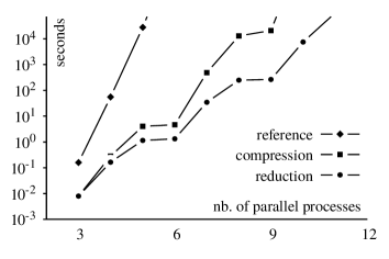
Figure 9. Impact of optimisations on verification time on Denning-Sacco.

Practical impact.

Finally, we illustrate how our optimisations make $\mathsf{Apte}$ much more useful in practice for investigating interesting scenarios. Verifying a single session of a protocol brings little assurance into its security. In order to detect replay attacks and to allow the attacker to compare messages that are exchanged, at least two sessions should be considered. This means having at least four parallel processes for two-party protocols, and six when a trusted third party is involved. This is actually beyond what the unoptimised $\mathsf{Apte}$ can handle in a reasonable amount of time. We show in Figure 10 how many parallel processes could be handled in $20$ hours by $\mathsf{Apte}$ on various use cases of protocols, for the same three variants of $\mathsf{Apte}$ as before, i.e. reference, compression and reduction. We verify an anonymity property for the Passive Authentication protocol of e-passports. For other protocols, we analyse strong secrecy of established keys: for one of the roles we add, on one side of the equivalence, an output encrypted by the established key and, on the other side, an output encrypted by a fresh key.

Protocol	reference	compression	reduction
Needham Schroeder (3-party)	4	6	7
Private Authentication (2-party)	4	7	7
Yahalom (3-party)	4	5	5
E-Passport PA (2-party)	4	7	9
Denning-Sacco (3-party)	5	9	10
Wide Mouth Frog (3-party)	6	12	13

Figure 10. Maximum number of parallel processes verifiable in 20 hours.

We finally present the benefits of our optimisations for discovering attacks. We performed some experiments on flawed variants of protocols, shown in Figure 11, corresponding to example files in subdirectory bench/protocols/attacks/ of the above mentioned release. The scenario Denning-Sacco A expresses strong secrecy of the (3-party) Denning-Sacco protocol, but this time on two instances of roles at the same time (instead of one as in Figure 10). In Denning-Sacco B, we consider again a form of strong secrecy expressed by outputting encrypted messages but this time at the end of role B. The Needham-Schroeder pub scenario corresponds to strong secrecy of the public-key Needham-Schroder protocol. The E-Passport PA exposed experiments show that anonymity is (obviously) lost with the Passive Authentication protocol when the secret key is made public. Similarly, the Yahalom exposed experiment shows that strong secrecy of Yahalom is lost when secrets keys are revealed. Since $\mathsf{Apte}$ stops its exploration as soon as an attack is found, the time needed for $\mathsf{Apte}$ to find the attack highly depends on the order in which the depth-first exploration is performed. However, as shown in Figure 11, we always observe in practice dramatic improvements brought by our optimisations compared to the reference version of $\mathsf{Apte}$. In some cases, our optimisations are even mandatory for $\mathsf{Apte}$ to find the attack using reasonable resources.

Protocol	reference	compression	reduction
Denning-Sacco A (6 par. proc.)	OoM	0.07s	0.02s
Denning-Sacco B (6 par. proc.)	5.83s	0.04s	0.04s
Needham-Shroeder pub (7 par. proc.)	TO	0.77s	0.67s
Needham-Shroeder pub (5 par. proc.)	0.79s	0.21s	0.13s
E-Passport PA exposed (8 par. proc.)	TO	0.02s	0.02s
E-Passport PA exposed (6 par. proc.)	4.37s	0.03s	0.02s
Yahalom exposed (4 par. proc.)	7.24s	0.02s	0.02s

Figure 11. Impact of optimisations for finding attacks (OoM denotes a consumption of $>$32Go of RAM and TO denotes a running time of $>$20 hours).

7. Related Work

The techniques we have presented borrow from standard ideas from concurrency theory and trace theory. Blending all these ingredients, and adapting them to the demanding framework of security protocols, we have come up with partial order reduction techniques that can effectively be used in symbolic verification algorithms for equivalence properties of security protocols. We now discuss related work, and there is a lot of it given the huge success of POR techniques in various application areas. We shall focus on the novel aspects of our approach, and explain why such techniques have not been needed outside of security protocol analysis. These observations are not new: as pointed out by Baier and Katoen [11], “[POR] is mainly appropriate to control-intensive applications and less suited for data-intensive applications”; Clarke et al. [25] also remark that “In the domain of model checking of reactive systems, there are numerous techniques for reducing the state space of the system. One such technique is partial-order reduction. This technique does not directly apply to [security protocol analysis] because we explicitly keep track of knowledge of various agents, and our logic can refer to this knowledge in a meaningful way.” We first compare our work with classical POR techniques, and then comment on previous work in the domain of security protocol analysis.

7.1. Classical POR

Partial order reduction techniques have proved very useful in the domain of model checking concurrent programs. Given a Labelled Transition System (LTS) and some property to check (e.g. a Linear Temporal Logic formula), the basic idea of POR [41, 34, 11] is to only consider a reduced version of the given LTS whose transitions of some states might be not exhaustive but are such that this transformation does not affect the property. POR techniques can be categorized in two groups [34]. First, the persistent set techniques (e.g. stubborn sets, ample sets) where only a sufficiently representative subset of available transitions is explored. Second, sleep set techniques memoize past exploration and use this information along with available transitions to disable some provably redundant transitions. Note that these two kinds of techniques are compatible, and are indeed often combined to obtain better reductions. Theoretical POR techniques apply to transition systems which may not be explicitly available in practice, or whose explicit computation may be too costly. In such cases, POR is often applied to an approximation of the LTS that is obtained through static analysis. Another, more recent approach is to use dynamic POR [31, 45, 3] where the POR arguments are applied based on information that is obtained during the execution of the system.

Clearly, classical POR techniques would apply to our concrete LTS, but that would not be practically useful since this LTS is wildly infinite, taking into account all recipes that the attacker could build. Applying most classical POR techniques to the LTS from which data would have been abstracted away would be ineffective: any input would be dependent on any output (since the attacker’s knowledge, increased by the output, may enable new input messages). Our compression technique lies between these two extremes. It exploits a semi-commutation property: outputs can be permuted before inputs, but not the converse in general. Further, it exploits the fact that inputs do not increase the attacker’s knowledge, and can thus be executed in a chained fashion, under focus. The semi-commutation is reminiscent of the asymmetrical dependency analysis enabled by the conditional stubborn set technique [34], and the execution of inputs under focus may be explained by means of sleep sets. While it may be possible to formally derive our compressed semantics by instantiating abstract POR techniques to our setting, we have not explored this possibility in detail. Concerning our reduced semantics, it may be seen as an application of the sleep set technique (or even as a reformulation of Anisimov’s and Knuth’s characterization of lexicographic normal forms) but the real contribution with this technique is to have formulated it in such a way (see Definition 5.1) that it can be implemented without requiring an a priori knowledge of data dependencies: it allows us to eliminate redundant traces on-the-fly as data (in)dependency is discovered by the constraint resolution procedure (as explained in Section 6.5)—in this sense, it may be viewed as a case of dynamic POR.

Narrowing the discussion a bit more, we now focus on the fact that our techniques are designed for the verification of equivalence properties. This requirement turns several seemingly trivial observations into subtle technical problems. For instance, ideas akin to compression are often applied without justification (e.g. in [44, 45, 40]) because they are obvious when one does reachability rather than equivalence checking. To understand this, it is important to distinguish between two very different ways of applying POR to equivalence checking (independently of the precise equivalence under consideration). The first approach is to reduce a system such that the reduced system and the original systems are equivalent. In the second approach, one only requires that two reduced systems are equivalent iff the original systems are equivalent. The first approach seems to be more common in the POR literature (where one finds, e.g. reductions that preserve LTL-satisfiability [11] or bisimilarity [37]) though there are instances of the second approach (e.g. for Petri nets [33]). In the present work, we follow the second approach: neither of our two reduction techniques preserves trace equivalence. This allows stronger reductions but requires extra care: one has to ensure that the independencies used in the reduction of one process are also meaningful for the other processes; in other words, reduction has to be symmetrical. We come back to these two different approaches later, when discussing specific POR techniques for security.

7.2. Security applications

The idea of applying POR to the verification of security protocols dates back, at least, to the work of Clarke et al. [25, 26]. In this work, the authors remark that traditional POR techniques cannot be directly applied to security mainly because “[they] must keep track of knowledge of various agents” and “[their] logic can refer to this knowledge in a meaningful way”. This led them to define a notion of semi-invisible actions (output actions, that cannot be swapped after inputs but only before them) and design a reduction that prioritizes outputs and performs them in a fixed order. Compared to our work, this reduction is much weaker (even weaker than compression only), only handles a finite set of messages, and only focuses on reachability properties checking.

In [30], the authors develop “state space reduction” techniques for the Maude-NRL Protocol Analyzer (Maude-NPA). This tool proceeds by backwards reachability analysis and treats at the same level the exploration of protocol executions and attacker’s deductions. Several reductions techniques are specific to this setting, and most are unrelated to partial order reduction in general, and to our work in particular. We note that the lazy intruder techniques from [30] should be compared to what is done in constraint resolution procedures (e.g. the one used in $\mathsf{Apte}$) rather than to our work. A simple POR technique used in Maude-NPA is based on the observation that inputs can be executed in priority in the backwards exploration, which corresponds to the fact that we can execute outputs first in forward explorations. We note again that this is only one aspect of the focused strategy, and that it is not trivial to lift this observation from reachability to trace equivalence. Finally, a “transition subsumption” technique is described for Maude-NPA. While highly non-trivial due to the technicalities of the model, this is essentially a tabling technique rather than a partial order reduction. Though it does yield a significant state space reduction (as shown in the experiments [30]) it falls short of exploiting independencies fully, and has a potentially high computational cost (which is not evaluated in the benchmarks of [30]).

In [32], Fokkink et al. model security protocols as labeled transition systems whose states contain the control points of different agents as well as previously outputted messages. They devise some POR technique for these transition systems, where output actions are prioritized and performed in a fixed order. In their work, the original and reduced systems are trace equivalent modulo outputs (the same traces can be found after removing output actions). The justification for their reduction would fail in our setting, where we consider standard trace equivalence with observable outputs. More importantly, their requirement that a reduced system should be equivalent to the original one makes it impossible to swap input actions, and thus reductions such as the execution under focus of our compressed semantics cannot be used. The authors leave as future work the problem of combining their algorithm with symbolic executions, in order to be able to lift the restriction to a finite number of messages.

Cremers and Mauw proposed [29] a reduction technique for checking secrecy in security protocols. Their method allows to perform outputs eagerly, as in our compressed semantics. It also uses a form of sleep set technique to avoid redundant interleavings of input actions. In addition to being applicable only for reachability property, the algorithm of [29] works under the assumption that for each input only finitely many input messages need to be considered. The authors identify as important future work the need to lift their method to the symbolic setting.

Earlier work by Mödersheim et al. has shown how to combine POR techniques with symbolic semantics [40] in the context of reachability properties for security protocols. This has led to high efficiency gains in the OFMC tool of the AVISPA platform [7]. While their reduction is very limited, it brings some key insight on how POR may be combined with symbolic execution. For instance, their reduction imposes a dependency constraint (called differentiation constraint in their work) on the interleavings of

$$\{\mathtt{in}(c,x).\mathtt{out}(c,m),\,\mathtt{in}(d,y).\mathtt{out}(d,m^{\prime})\}.$$

Assuming that priority is given to the process working on channel $c$, this constraint enforces that any symbolic interleaving of the form ${\mathtt{in}(d,M^{\prime}).\mathtt{out}(d,w^{\prime}).\mathtt{in}(c,M).\mathtt{out}(c,w)}$ would only be explored for instances of $M$ that depend on $w^{\prime}$. Our reduced semantics constrains patterns of arbitrary size (instead of just size 2 diamond patterns as above) by means of dependency constraints. Going back to Example 5.1, their technique will only be able (at most) to exploit the dependencies depicted in plain blue arrows, and they will not consider the one represented by the dashed 2-arrow. Moreover, while we generate dependency constraints on the fly, they implement their technique by looking for such a pattern afterwards. This causes a tradeoff between reduction and the cost of redundancy detection: their technique fails to detect all patterns of this kind. Besides these differences, we note that Mödersheim et al. use dependency constraints to guide a dedicated constraint resolution procedure, while we chose to treat constraint resolution (almost) as a black box, and leave it unchanged. Finally, we recall that our POR technique has been designed to be sound and complete for trace equivalence checking as well as reachability checking.

Finally, in [10], the authors of the present paper extend some of the results presented here. Instead of considering the syntactic fragment of simple processes, we work under the more general semantical assumption of action-determinism. We show that compression and reduction can be extended to that case, preserving the main result: the induced equivalences coincide. However, that work is completely carried out in concrete rather than symbolic semantics. Thus, this development should be viewed as being orthogonal to the one carried out in the present paper. The main ideas behind the integration in symbolic semantics and $\mathsf{Apte}$ would apply to the action-deterministic case as well. The line of research followed in [10], that consists in extending the supported fragment for our POR techniques, is still open: it would be interesting to support processes that are not action-deterministic, which are commonplace when analysing anonymity or unlinkability scenarios.

8. Conclusion

We have developed two POR techniques that are adequate for verifying trace equivalence properties between simple processes. The first refinement groups actions in blocks, while the second one uses dependency constraints to restrict to minimal interleavings among a class of permutations. In both cases, the refined semantics has less traces, yet we show that the associated trace equivalence coincides with the standard one. We have effectively implemented these refinements in $\mathsf{Apte}$, and shown that they yield the expected, significant benefit.

We claim that our POR techniques – at least compression – and the significant optimisations they allow are generic enough to be applicable to other verification methods as long as they perform forward symbolic executions. In addition to the integration in Apte we have extensively discussed, we also have successfully done so in Spec [35]. Furthermore, parts of our POR techniques have been independently integrated and implemented in the distributed version of $\mathsf{Akiss}$ .

We are considering several directions for future work. Regarding the theoretical results presented here, it is actually possible to slightly relax the syntactic condition we imposed on processes by an action-determinism hypothesis and apply our reduction techniques on replicated processes [10]. The question of whether the action-determinism condition can be removed without degrading the reductions too much is left open. Another interesting direction would be to adapt our techniques for verification methods based on backward search instead of forward search as is the case in this paper. We also believe that stronger reductions can be achieved: for instance, exploiting symmetries should be very useful for dealing with multiple sessions. Regarding the practical application of our results, we can certainly go further. We could investigate the role of the particular choice of the order $\prec$, to determine heuristics for maximising the practical impact of reduction.

Acknowledgements

We would like to thank Vincent Cheval for interesting discussions and comments, especially on Section 6.

Appendix A Notations

Symbol	Description	Reference
$\mathrel{\raisebox{-0.5pt}[5.0pt]{$\xrightarrow{\raisebox{-1.2pt}[2.0pt][1.0pt]{\scalebox{0.7}{$$}}}$}}$	transition for concrete processes	Figure 2
$\ext@arrow 0{13}{15}8\Rightarrowfill@{}{}$	$\mathrel{\raisebox{-0.5pt}[5.0pt]{$\xrightarrow{\raisebox{-1.2pt}[2.0pt][1.0pt]{\scalebox{0.7}{$$}}}$}}$ up-to non-observable actions	Section 2.2
$\sim$	static equivalence	Definition 2.3
$\sqsubseteq$	trace inclusion for concrete processes	Definition 2.3
$\approx$	trace equivalence for concrete processes	Definition 2.3
$\ext@arrow 3{15}59\arrowfill@\relbar\relbar\rightarrow\mkern-10.0mu\joinrel\rightarrow{}$	focused semantics	Figure 3
$\mathrel{\raisebox{-0.5pt}[5.0pt]{$\xrightarrow{\raisebox{-1.2pt}[2.0pt][1.0pt]{\scalebox{0.7}{$$}}}$}}_{c}$	compressed semantics	Figure 4
$\sqsubseteq_{c}$	trace inclusion induced by $\mathrel{\raisebox{-0.5pt}[5.0pt]{$\xrightarrow{\raisebox{-1.2pt}[2.0pt][1.0pt]{\scalebox{0.7}{$$}}}$}}_{c}$	Definition 3.1
$\approx_{c}$	trace equivalence induced by $\mathrel{\raisebox{-0.5pt}[5.0pt]{$\xrightarrow{\raisebox{-1.2pt}[2.0pt][1.0pt]{\scalebox{0.7}{$$}}}$}}_{c}$	Definition 3.1
$\mathrel{\raisebox{-0.5pt}[5.0pt]{$\xmapsto{\raisebox{-1.2pt}[2.0pt][1.0pt]{\scalebox{0.7}{$$}}}$}}$	symbolic semantics	Figure 5
$\ext@arrow 3{15}59\arrowfill@{\mapstochar\relbar}\relbar\rightarrow\mkern-10.0mu\joinrel\rightarrow{}$	focused symbolic semantics	Figure 6
$\mathrel{\raisebox{-0.5pt}[5.0pt]{$\xmapsto{\raisebox{-1.2pt}[2.0pt][1.0pt]{\scalebox{0.7}{$$}}}$}}_{c}$	compressed symbolic semantics	Figure 6
$\sqsubseteq^{s}$	trace inclusion induced by $\mathrel{\raisebox{-0.5pt}[5.0pt]{$\xmapsto{\raisebox{-1.2pt}[2.0pt][1.0pt]{\scalebox{0.7}{$$}}}$}}$	Definition 4.2
$\sqsubseteq_{c}^{s}$	trace inclusion induced by $\mathrel{\raisebox{-0.5pt}[5.0pt]{$\xmapsto{\raisebox{-1.2pt}[2.0pt][1.0pt]{\scalebox{0.7}{$$}}}$}}_{c}$	Definition 4.2
$\approx^{s}$	trace equivalence induced by $\mathrel{\raisebox{-0.5pt}[5.0pt]{$\xmapsto{\raisebox{-1.2pt}[2.0pt][1.0pt]{\scalebox{0.7}{$$}}}$}}$	Definition 4.2
$\approx^{s}_{c}$	trace equivalence induced by $\mathrel{\raisebox{-0.5pt}[5.0pt]{$\xmapsto{\raisebox{-1.2pt}[2.0pt][1.0pt]{\scalebox{0.7}{$$}}}$}}_{c}$	Definition 4.2
$\overrightarrow{X}\mathbb{n}\overrightarrow{w}$	dependency constraint	Definition 5.1
$\mathrm{Deps}\left(\mathsf{tr}\right)$	dependency constraints induced by a trace	Definition 5.1
$\sqsubseteq_{r}^{s}$	trace inclusion up-to dependency constraints	Definition 5.1
$\approx^{s}_{r}$	trace equivalence up-to dependency constraints	Definition 5.1
$\mid\mid$	independence of blocks	Definition 5.2
$\equiv_{\Phi}$	equivalence of two traces	Definition 5.2
$\lceil{(\mathcal{P};\Phi;\mathcal{S})}\rceil$	associated extented symbolic process	Section 6.1
$\lfloor{\left(\mathcal{P};\Phi;\mathcal{S};\mathcal{S}^{+}\right)}\rfloor$	associated symbolic process	Section 6.1
$\prec^{+}$	symbolic inclusion of sets of extended symbolic processes	Definition 6.1
$\sim^{+}$	symbolic equivalence of sets of extended symbolic processes	Definition 6.1
$\mathrel{\raisebox{-0.5pt}[5.0pt]{$\xmapsto{\raisebox{-1.2pt}[2.0pt][1.0pt]{\scalebox{0.7}{$$}}}$}}^{\mathsf{A}}$	$\mathsf{Apte}$ exploration step	Section 6.1
$\mathrel{\raisebox{-0.5pt}[5.0pt]{$\xmapsto{\raisebox{-1.2pt}[2.0pt][1.0pt]{\scalebox{0.7}{$$}}}$}}^{\mathsf{A1}}$	first part of $\mathsf{Apte}$ exploration step	Section 6.1
$\mathrel{\raisebox{-0.5pt}[5.0pt]{$\xmapsto{\raisebox{-1.2pt}[2.0pt][1.0pt]{\scalebox{0.7}{$$}}}$}}^{\mathsf{A2}}{}$	second part of $\mathsf{Apte}$ exploration step	Section 6.1
$\mathrel{\raisebox{-0.5pt}[5.0pt]{$\xmapsto{\raisebox{-1.2pt}[2.0pt][1.0pt]{\scalebox{0.7}{$$}}}$}}_{c}^{\mathsf{A}}$	compressed version of $\mathrel{\raisebox{-0.5pt}[5.0pt]{$\xmapsto{\raisebox{-1.2pt}[2.0pt][1.0pt]{\scalebox{0.7}{$$}}}$}}^{\mathsf{A}}$	Section 6.4
$\mathrel{\raisebox{-0.5pt}[5.0pt]{$\xmapsto{\raisebox{-1.2pt}[2.0pt][1.0pt]{\scalebox{0.7}{$$}}}$}}_{r}^{\mathsf{A}}$	reduced version of $\mathrel{\raisebox{-0.5pt}[5.0pt]{$\xmapsto{\raisebox{-1.2pt}[2.0pt][1.0pt]{\scalebox{0.7}{$$}}}$}}_{c}^{\mathsf{A}}$	Section 6.5
$\approx^{\mathsf{A}}$	equivalence induced by $\mathrel{\raisebox{-0.5pt}[5.0pt]{$\xmapsto{\raisebox{-1.2pt}[2.0pt][1.0pt]{\scalebox{0.7}{$$}}}$}}^{\mathsf{A}}$	Definition 6.1
$\approx^{\mathsf{A}}_{c}$	equivalence induced by $\mathrel{\raisebox{-0.5pt}[5.0pt]{$\xmapsto{\raisebox{-1.2pt}[2.0pt][1.0pt]{\scalebox{0.7}{$$}}}$}}_{c}^{\mathsf{A}}$	Section 6.4
$\approx^{\mathsf{A}}_{r}$	equivalence induced by $\mathrel{\raisebox{-0.5pt}[5.0pt]{$\xmapsto{\raisebox{-1.2pt}[2.0pt][1.0pt]{\scalebox{0.7}{$$}}}$}}_{r}^{\mathsf{A}}$	Section 6.5

Appendix B Proofs of Section 3

See 3.2

Proof.

It suffices to establish that $A\xRightarrow{\alpha\cdot\alpha^{\prime}\;}A^{\prime}$ implies $A\xRightarrow{\alpha^{\prime}\cdot\alpha\;}A^{\prime}$ for any $\alpha\;{\mathrel{\mathcal{I}}}_{a}\;\alpha^{\prime}$.

• Assume that we have $A\xRightarrow{\mathtt{out}(c_{i},w_{i})}A_{i}\xRightarrow{\mathtt{out}(c_{j},w_{j})}A^{\prime}$ with $c_{i}\neq c_{j}$. Because we are considering simple processes, the two actions must be concurrent. More specifically, our process $A$ must be of the form $(\{P_{i},P_{j}\}\uplus\mathcal{P}_{r};\Phi)$ with $P_{i}$ (resp. $P_{j}$) being a basic process on channel $c_{i}$ (resp. $c_{j}$). We assume that in our sequence of reductions, $\tau$ actions pertaining to $P_{i}$ are all executed before reaching $A_{i}$, and that $\tau$ actions pertaining to $\mathcal{P}_{r}$ are executed last. This is without loss of generality, because a $\tau$ action on a given basic process can easily be permuted with actions taking place on another basic process, since it does not depend on the context and has no effect on the frame. Thus we have that $A_{i}=(\{P^{\prime}_{i},P_{j}\}\uplus\mathcal{P}_{r};\Phi\uplus\{w_{i}\triangleright m_{i}\})$, $A^{\prime}=(\{P^{\prime}_{i};P^{\prime}_{j}\}\uplus\mathcal{P}^{\prime}_{r};\Phi\uplus\{w_{i}\triangleright m_{i},w_{j}\triangleright m_{j}\})$. Since the $\tau$ actions taking place on $\mathcal{P}^{\prime}_{r}$ rely neither on the frame nor on the first two basic processes, we easily obtain the permuted execution:

  $$\begin{array}[]{rcl}A&\xRightarrow{\mathtt{out}(c_{j},w_{j})}&(\{P_{i},P^{\prime}_{j}\}\uplus\mathcal{P}_{r};\Phi\uplus\{w_{j}\triangleright m_{j}\})\\ &\xRightarrow{\mathtt{out}(c_{i},w_{i})}&(\{P^{\prime}_{i},P^{\prime}_{j}\}\uplus\mathcal{P}^{\prime}_{r};\Phi\uplus\{w_{i}\triangleright m_{i},w_{j}\triangleright m_{j}\})\end{array}$$

• The permutation of two input actions on distinct channels is very similar. In this case, the frame does not change at all, and the order in which messages are derived from the frame does not matter. Moreover, the instantiation of the input variable on one basic process has no impact on the other ones.

• Assume that we have $A\xRightarrow{\mathtt{out}(c_{i},w_{i})}A_{i}\xRightarrow{\mathtt{in}(c_{j},M)}A^{\prime}$ with $c_{i}\neq c_{j}$ and $w_{i}\not\in\mathit{fv}(M)$. Again, the two actions are concurrent, and we can assume that $\tau$ actions are organized conveniently so that $A$ is of the form $(\{P_{i},P_{j}\}\uplus\mathcal{P}_{r};\Phi)$ with $P_{i}$ (resp. $P_{j}$) a basic process on $c_{i}$ (resp. $c_{j}$); $A_{i}$ is of the form $(\{P^{\prime}_{i},P_{j}\}\uplus\mathcal{P}_{r};\Phi\uplus\{w_{i}\triangleright m_{i}\})$; and $A^{\prime}$ is of the form $(\{P^{\prime}_{i},P^{\prime}_{j}\}\uplus\mathcal{P}^{\prime}_{r};\Phi\uplus\{w_{i}\triangleright m_{i}\})$. As before, the $\tau$ actions from $\mathcal{P}_{r}$ to $\mathcal{P}^{\prime}_{r}$ are easily moved around. Additionally, $w_{i}\not\in\mathit{fv}(M)$ implies $\mathit{fv}(M)\subseteq\mathrm{dom}(\Phi)$ and thus we have:

  $$(\{P_{i},P_{j}\}\uplus\mathcal{P}_{r};\Phi)\xRightarrow{\mathtt{in}(c_{j},M)}(\{P_{i},P^{\prime}_{j}\}\uplus\mathcal{P}_{r};\Phi)$$

  The next step is trivial:

  $$(\{P_{i},P^{\prime}_{j}\}\uplus\mathcal{P}_{r};\Phi)\xRightarrow{\mathtt{out}(c_{i},w_{i})}(\{P^{\prime}_{i},P^{\prime}_{j}\}\uplus\mathcal{P}^{\prime}_{r};\Phi\uplus\{w_{i}\triangleright m_{i}\})$$

• We also have to perform the reverse permutation, but we shall not detail it; this time we are delaying the derivation of $M$ from the frame, and it only gets easier.∎

See 3.2

Proof.

We first observe that $A\xRightarrow{\mathsf{tr}}A^{\prime}$ implies $A\ext@arrow 3{15}59\arrowfill@\relbar\relbar\rightarrow\mkern-10.0mu\joinrel\rightarrow{}{\mathsf{tr}}_{o^{*}}A^{\prime}$ if $A^{\prime}$ is initial and $\mathsf{tr}$ is a (possibly empty) sequence of output actions on the same channel. We prove this by induction on the sequence of actions. If it is empty, we can conclude using one of the Proper rules because $A=A^{\prime}$ is initial. Otherwise, we have:

$$A\xRightarrow{\mathtt{out}(c,w)}A^{\prime\prime}\xRightarrow{\mathsf{tr}\;}A^{\prime}.$$

We obtain $A^{\prime\prime}\ext@arrow 3{15}59\arrowfill@\relbar\relbar\rightarrow\mkern-10.0mu\joinrel\rightarrow{}{\mathsf{tr}}_{o^{*}}A^{\prime}$ by induction hypothesis, and conclude using rules Tau and Out.

The next step is to show that $A\xRightarrow{\mathsf{tr}\;}A^{\prime}$ implies $A\ext@arrow 3{15}59\arrowfill@\relbar\relbar\rightarrow\mkern-10.0mu\joinrel\rightarrow{}{\mathsf{tr}}_{i^{*}}A^{\prime}$, if $A^{\prime}$ is initial and $\mathsf{tr}$ is the concatenation of a (possibly empty) sequence of inputs and a non-empty sequence of outputs, all on the same channel. This is easily shown by induction on the number of input actions. If there are none we use the previous result, otherwise we conclude by induction hypothesis and using rules Tau and In. Otherwise, the first output action allows us to conclude from the previous result and rules Tau and Out.

We can now show that $A\xRightarrow{\mathsf{tr}\;}A^{\prime}$ implies $A\ext@arrow 3{15}59\arrowfill@\relbar\relbar\rightarrow\mkern-10.0mu\joinrel\rightarrow{}{\mathsf{tr}}_{i^{+}}A^{\prime}$ if $A^{\prime}$ is initial and $\mathsf{tr}$ is a proper block. Indeed, we must have

$$A\xRightarrow{\mathtt{in}(c,M)}A^{\prime\prime}\xRightarrow{\mathsf{tr}^{\prime}\;}A^{\prime}$$

which allows us to conclude using the previous result and rules Tau and In.

We finally obtain that $A\xRightarrow{\mathsf{tr}}A^{\prime}$ implies $A\mathrel{\raisebox{-0.5pt}[5.0pt]{$\xrightarrow{\raisebox{-1.2pt}[2.0pt][1.0pt]{\scalebox{0.7}{$\mathsf{tr}$}}}$}}_{c}A^{\prime}$ when $A$ and $A^{\prime}$ are initial simple processes and $\mathsf{tr}$ is a sequence of proper blocks. This is done by induction on the number of blocks. The base case is trivial. Because $A$ is initial, the execution of its basic processes can only start with observable actions, thus only one basic process is involved in the execution of the first block. Moreover, we can assume without loss of generality that the execution of this first block results in another initial process: indeed the basic process resulting from that execution is either in the final process $A^{\prime}$, which is initial, or it will perform another block, i.e. it can perform $\tau$ actions followed by an input, in which case we can force those $\tau$ actions to take place as early as possible. Thus we have

$$A\xRightarrow{\mathsf{b}}A^{\prime\prime}\xRightarrow{\mathsf{tr}^{\prime}}A^{\prime}$$

where $\mathsf{b}$ is a proper block, and we conclude using the previous result and the induction hypothesis. ∎

Before proving Theorem 3.2, we establish the following result.

Proposition .

Let $\mathsf{tr}$ be a trace of observable actions such that, for any channel $c$ occurring in the trace, it appears first in an input action. There exists a sequence of proper blocks $\mathsf{tr}_{io}$ and a sequence of improper blocks $\mathsf{tr}_{i}$ such that $\mathsf{tr}=_{{\mathrel{\mathcal{I}}}_{a}}\mathsf{tr}_{io}\cdot\mathsf{tr}_{i}$.

Proof.

We proceed by induction on the length of $\mathsf{tr}$, and distinguish two cases:

• If $\mathsf{tr}$ has no output action then, by swapping input actions on distinct channels, we reorder $\mathsf{tr}$ so as to obtain $\mathsf{tr}_{i}=\mathsf{tr}^{c_{1}}\cdot\ldots\cdot\mathsf{tr}^{c_{n}}=_{{\mathrel{\mathcal{I}}}_{a}}\mathsf{tr}$ where the $c_{i}$’s are pairwise distinct and $\mathsf{tr}^{c_{i}}$ is an improper block on channel $c_{i}$.

• Otherwise, there must be a decomposition $\mathsf{tr}=\mathsf{tr}_{1}\cdot\mathtt{out}(c,w)\cdot\mathsf{tr}_{2}$ such that $\mathsf{tr}_{1}$ does not contain any output. We can perform swaps involving input actions of $\mathsf{tr}_{1}$ on all channel $c^{\prime}\neq c$, so that they are delayed after the first output on $c$. We obtain $\mathsf{tr}=_{{\mathrel{\mathcal{I}}}_{a}}\mathtt{in}(c,M_{1})\cdot\ldots\cdot\mathtt{in}(c,M_{n})\cdot\mathtt{out}(c,w)\cdot\mathsf{tr}_{1}^{\prime}\cdot\mathsf{tr}_{2}$ with $n\geq 1$. Next, we swap output actions on channel $c$ from $\mathsf{tr}_{1}^{\prime}\cdot\mathsf{tr}_{2}$ that are not preceded by another input on $c$, so as to obtain

  $$\mathsf{tr}=_{{\mathrel{\mathcal{I}}}_{a}}\mathtt{in}(c,M_{1})\dots\mathtt{in}(c,M_{n})\cdot\mathtt{out}(c,w)\cdot\mathtt{out}(c,w_{1})\dots\mathtt{out}(c,w_{m})\cdot\mathsf{tr}_{2}^{\prime}$$

  such that either $\mathsf{tr}_{2}^{\prime}$ does not contain any action on channel $c$ or the first one is an input action. We have thus isolated a first proper block, and we can conclude by induction hypothesis on $\mathsf{tr}_{2}^{\prime}$.∎

Note that the above result does not exploit all the richness of ${\mathrel{\mathcal{I}}}_{a}$. In particular, it never relies on the possibility to swap an input action before an output when the input message does not use the output handled. Indeed, the idea behind compression does not rely on messages. This is no longer the case in Section 5 where we use ${{\mathrel{\mathcal{I}}}_{a}}$ more fully.

We finally prove the main result about the compressed semantics relying on Proposition B stated and proved above. Given two simple process $A=(\mathcal{P};\Phi)$ and $A^{\prime}=(\mathcal{P}^{\prime};\Phi^{\prime})$, we shall write $\Phi(A)\sim\Phi(A^{\prime})$ (or even $A\sim A^{\prime}$) instead of $\Phi\sim\Phi^{\prime}$.

See 3.2

Proof.

We prove the two directions separately.

$(\Rightarrow)$ Let $A$ be an initial simple process such that $A\approx B$ and ${A\mathrel{\raisebox{-0.5pt}[5.0pt]{$\xrightarrow{\raisebox{-1.2pt}[2.0pt][1.0pt]{\scalebox{0.7}{$\mathsf{tr}$}}}$}}_{c}A^{\prime}}$. One can easily see that the trace $\mathsf{tr}$ must be of the form $\mathsf{tr}_{io}\cdot\mathsf{tr}_{i}$ where $\mathsf{tr}_{io}$ is made of proper blocks and $\mathsf{tr}_{i}$ is a (possibly empty) sequence of inputs on the same channel $c_{j}$. We have:

$$A\mathrel{\raisebox{-0.5pt}[5.0pt]{$\xrightarrow{\raisebox{-1.2pt}[2.0pt][1.0pt]{\scalebox{0.7}{$\mathsf{tr}_{io}$}}}$}}_{c}A^{\prime\prime}\mathrel{\raisebox{-0.5pt}[5.0pt]{$\xrightarrow{\raisebox{-1.2pt}[2.0pt][1.0pt]{\scalebox{0.7}{$\mathsf{tr}_{i}$}}}$}}_{c}A^{\prime}$$

Using Proposition 3.2, we obtain that $A\xRightarrow{\mathsf{tr}_{io}}A^{\prime\prime}$. We also claim that $A^{\prime\prime}\xRightarrow{\mathsf{tr}_{i}}A^{+}$ for some $A^{+}$ having the same frame as $A^{\prime}$ which is itself equal to the one of $A^{\prime\prime}$. This is obvious when $\mathsf{tr}_{i}$ is empty—in that case we can simply choose $A^{+}=A^{\prime}=A^{\prime\prime}$. Otherwise, the execution of the improper block $\mathsf{tr}_{i}$ results from the application of rule Improper. Except for the fact that this rule “kills” the resulting process, its subderivation simply packages a sequence of inputs, and so we have a suitable $A^{+}$. We thus have:

$$A\xRightarrow{\mathsf{tr}_{io}\;}A^{\prime\prime}\xRightarrow{\mathsf{tr}_{i}\;}A^{+}$$

By hypothesis, it implies that $B\xRightarrow{\mathsf{tr}_{io}\;}B^{\prime\prime}$ and $B\xRightarrow{\mathsf{tr}_{io}\cdot\mathsf{tr}_{i}\;}B^{+}$ with $A^{\prime\prime}\sim B^{\prime\prime}$ and ${A^{+}\sim B^{+}}$. Relying on the fact that $B$ is a simple process, we have:

$$B\xRightarrow{\mathsf{tr}_{io}}B^{\prime\prime}\xRightarrow{\mathsf{tr}_{i}}B^{+}$$

It remains to establish that $B\mathrel{\raisebox{-0.5pt}[5.0pt]{$\xrightarrow{\raisebox{-1.2pt}[2.0pt][1.0pt]{\scalebox{0.7}{$\mathsf{tr}$}}}$}}_{c}B^{\prime}$ such that $B^{\prime}\sim A^{\prime}$. We can assume that $B^{\prime\prime}$ does not have any basic process starting with a test, without loss of generality since forcing $\tau$ actions cannot break static equivalence. Further, we observe that $B^{\prime\prime}$ is initial. Otherwise, it would mean that a basic process of $B$ is not initial (absurd) or that one of the blocks of $\mathsf{tr}_{io}$, which are maximal for $A$, is not maximal for $B$ (absurd again, because it contradicts $A\approx B$). This allows us to apply Proposition 3.2 to obtain

$$B\mathrel{\raisebox{-0.5pt}[5.0pt]{$\xrightarrow{\raisebox{-1.2pt}[2.0pt][1.0pt]{\scalebox{0.7}{$\mathsf{tr}_{io}$}}}$}}_{c}B^{\prime\prime}.$$

This concludes when $\mathsf{tr}_{i}$ is empty, because $B^{\prime}=B^{\prime\prime}\sim A^{\prime\prime}=A^{\prime}$. Otherwise, we note that $A^{+}$ cannot perform any action on channel $c_{j}$, because the execution of $\mathsf{tr}_{i}$ in the compressed semantics must be maximal. Since $A\approx B$, it must be that $B^{+}$ cannot perform any observable action on the channel $c_{j}$ either. Thus $B^{\prime\prime}$ can complete an improper step:

$$B^{\prime\prime}\mathrel{\raisebox{-0.5pt}[5.0pt]{$\xrightarrow{\raisebox{-1.2pt}[2.0pt][1.0pt]{\scalebox{0.7}{$\mathsf{tr}_{i}$}}}$}}_{c}B^{\prime}\mbox{ where }B^{\prime}=(\emptyset;\Phi(B^{+})).$$

We can finally conclude that $B\mathrel{\raisebox{-0.5pt}[5.0pt]{$\xrightarrow{\raisebox{-1.2pt}[2.0pt][1.0pt]{\scalebox{0.7}{$\mathsf{tr}$}}}$}}_{c}B^{\prime}$ with $\Phi(B^{\prime})=\Phi(B^{+})\sim\Phi(A^{+})=\Phi(A^{\prime})$.

$(\Leftarrow)$ Let $A$ be an initial simple process such that $A\approx_{c}B$ and $A\xRightarrow{\mathsf{tr}}A^{\prime}$. We “complete” this execution as follows:

• We force $\tau$ actions whenever possible.

• If the last action on $c$ in $\mathsf{tr}$ is an input, we trigger available inputs on $c$ using a valid public constant as a recipe.

• We trigger all the outputs that are available and not blocked.

We obtain a trace of the form $\mathsf{tr}\cdot\mathsf{tr}^{+}$. Let $A^{+}$ be the process obtained from this trace:

$$A\xRightarrow{\mathsf{tr}}A^{\prime}\xRightarrow{\mathsf{tr}^{+}}A^{+}$$

We observe that $A^{+}$ is initial. Indeed, for each basic process that performs actions in $\mathsf{tr}\cdot\mathsf{tr}^{+}$, we have that:

• either the last action on its channel is an output and the basic process is of the form $\mathtt{in}(c,\_).P$ or $\mathtt{out}(c,u).P$ with $\neg\mathit{valid}(u)$,

• or the last action is an input and the basic process is reduced to $0$ and disappears, or it is an output which is blocked.

Next, we apply Proposition B to obtain traces $\mathsf{tr}_{sio}$ (resp. $\mathsf{tr}_{i}$) made of proper (resp. improper) blocks, such that $\mathsf{tr}\cdot\mathsf{tr}^{+}=_{{\mathrel{\mathcal{I}}}_{a}}\mathsf{tr}_{io}\cdot\mathsf{tr}_{i}$. By Lemma 3.2 we know that this permuted trace can also lead to $A^{+}$:

$$A\xRightarrow{\mathsf{tr}_{io}}A_{io}\xRightarrow{\mathsf{tr}_{i}}A^{+}$$

As before, we can assume that $A_{io}$ cannot perform any $\tau$ action. Under this condition, since $A^{+}$ is initial, $A_{io}$ must also be initial.

By Proposition 3.2 we have that $A\mathrel{\raisebox{-0.5pt}[5.0pt]{$\xrightarrow{\raisebox{-1.2pt}[2.0pt][1.0pt]{\scalebox{0.7}{$\mathsf{tr}_{io}$}}}$}}_{c}A_{io}$, and $A\approx_{c}B$ implies that:

$$B\mathrel{\raisebox{-0.5pt}[5.0pt]{$\xrightarrow{\raisebox{-1.2pt}[2.0pt][1.0pt]{\scalebox{0.7}{$\mathsf{tr}_{io}$}}}$}}_{c}B_{io}\mbox{ with }\Phi(A_{io})\sim\Phi(B_{io}).$$

A simple inspection of the Proper rules shows that a basic process resulting from the execution of a proper block must be initial. Thus, since the whole simple process $B$ is initial, $B_{io}$ is initial too.

Thanks to Proposition 3.2, we have that $B\xRightarrow{\mathsf{tr}_{io}}B_{io}$. Our goal is now to prove that we can complete this execution with $\mathsf{tr}_{i}$. This trace is of the form $\mathsf{tr}^{c_{1}}\cdot\mathsf{tr}^{c_{2}}\dots\mathsf{tr}^{c_{n}}$ where $\mathsf{tr}^{c_{i}}$ contains only inputs on channel $c_{i}$ and the $c_{i}$ are pairwise disjoint. Now, we easily see that for each $i$,

$$A_{io}\xRightarrow{\mathsf{tr}^{c_{i}}}A_{i}$$

and $A_{i}$ has no more atomic process on channel $c_{i}$. Thus we have $A_{io}\mathrel{\raisebox{-0.5pt}[5.0pt]{$\xrightarrow{\raisebox{-1.2pt}[2.0pt][1.0pt]{\scalebox{0.7}{$\mathsf{tr}^{c_{i}}$}}}$}}_{c}A_{i}^{0}$ with $A_{i}^{0}=(\emptyset;\Phi(A_{i}))$. Since $A\approx_{c}B$, we must have some $B_{i}^{0}$ such that:

$$B\mathrel{\raisebox{-0.5pt}[5.0pt]{$\xrightarrow{\raisebox{-1.2pt}[2.0pt][1.0pt]{\scalebox{0.7}{$\mathsf{tr}_{io}$}}}$}}_{c}B_{io}\mathrel{\raisebox{-0.5pt}[5.0pt]{$\xrightarrow{\raisebox{-1.2pt}[2.0pt][1.0pt]{\scalebox{0.7}{$\mathsf{tr}^{c_{i}}$}}}$}}_{c}B_{i}^{0}$$

We can translate this back to the regular semantics, obtaining $B\xRightarrow{\mathsf{tr}_{io}}B_{io}\xRightarrow{\mathsf{tr}^{c_{i}}}B_{i}$. We can now execute all these inputs to obtain an execution of $\mathsf{tr}_{io}\cdot\mathsf{tr}_{i}$ towards some process $B^{+}$:

$$B\xRightarrow{\mathsf{tr}_{io}}B_{io}\xRightarrow{\mathsf{tr}_{i}}B^{+}$$

Permuting those actions, we obtain thanks to Lemma 3.2:

$$B\xRightarrow{\mathsf{tr}}B^{\prime}\xRightarrow{\mathsf{tr}^{+}}B^{+}$$

We observe that $\Phi(B^{+})=\Phi(B_{io})\sim\Phi(A_{io})\sim\Phi(A^{+})$, and it follows that ${A^{\prime}\sim B^{\prime}}$ because those frames have the same domain, which is a subset of that of ${\Phi(A^{+})\sim\Phi(B^{+})}$. ∎

References

• [1] M. Abadi and C. Fournet. Mobile values, new names, and secure communication. In Proc. 28th Symposium on Principles of Programming Languages (POPL’01), pages 104–115. ACM Press, 2001.
• [2] M. Abadi and C. Fournet. Private authentication. Theoretical Computer Science, 322(3):427–476, 2004.
• [3] P. Abdulla, S. Aronis, B. Jonsson, and K. Sagonas. Optimal dynamic partial order reduction. ACM SIGPLAN Notices, 49(1):373–384, 2014.
• [4] J.-M. Andreoli. Logic programming with focusing proofs in linear logic. J. Log. Comput., 2(3), 1992.
• [5] M. Arapinis, T. Chothia, E. Ritter, and M. Ryan. Analysing unlinkability and anonymity using the applied pi calculus. In Proc. 23rd Computer Security Foundations Symposium (CSF’10), pages 107–121. IEEE Comp. Soc. Press, 2010.
• [6] A. Armando, R. Carbone, L. Compagna, J. Cuellar, and L. T. Abad. Formal analysis of saml 2.0 web browser single sign-on: Breaking the saml-based single sign-on for google apps. In Proc. 6th ACM Workshop on Formal Methods in Security Engineering (FMSE 2008), pages 1–10, 2008.
• [7] A. Armando et al. The AVISPA Tool for the automated validation of internet security protocols and applications. In Proc. 17th Int. Conference on Computer Aided Verification (CAV’05), LNCS. Springer, 2005.
• [8] A. Armando et al. The AVANTSSAR platform for the automated validation of trust and security of service-oriented architectures. In Tools and Algorithms for the Construction and Analysis of Systems - 18th International Conference, TACAS 2012, Held as Part of the European Joint Conferences on Theory and Practice of Software, ETAPS 2012, Tallinn, Estonia, March 24 - April 1, 2012. Proceedings, pages 267–282, 2012.
• [9] D. Baelde, S. Delaune, and L. Hirschi. A reduced semantics for deciding trace equivalence using constraint systems. In Proc. of POST’14. Springer, 2014.
• [10] D. Baelde, S. Delaune, and L. Hirschi. Partial order reduction for security protocols. In L. Aceto and D. de Frutos-Escrig, editors, Proceedings of the 26th International Conference on Concurrency Theory (CONCUR’15), volume 42 of Leibniz International Proceedings in Informatics, pages 497–510, Madrid, Spain, Sept. 2015. Leibniz-Zentrum für Informatik.
• [11] C. Baier and J.-P. Katoen. Principles of Model Checking (Representation and Mind Series). The MIT Press, 2008.
• [12] M. Baudet. Deciding security of protocols against off-line guessing attacks. In Proc. 12th Conference on Computer and Communications Security. ACM, 2005.
• [13] B. Blanchet. An Efficient Cryptographic Protocol Verifier Based on Prolog Rules. In Proc. 14th Computer Security Foundations Workshop (CSFW’01), pages 82–96. IEEE Comp. Soc. Press, 2001.
• [14] B. Blanchet, M. Abadi, and C. Fournet. Automated verification of selected equivalences for security protocols. Journal of Logic and Algebraic Programming, 2008.
• [15] R. Chadha, Ş. Ciobâcă, and S. Kremer. Automated verification of equivalence properties of cryptographic protocols. In Proc. 21th European Symposium on Programming Languages and Systems (ESOP’12), LNCS. Springer, 2012.
• [16] R. Chadha, Ş. Ciobâcă, and S. Kremer. Automated verification of equivalence properties of cryptographic protocols. In Programming Languages and Systems, pages 108–127. Springer, 2012.
• [17] V. Cheval. APTE: http://projects.lsv.ens-cachan.fr/APTE/, 2011.
• [18] V. Cheval. Automatic verification of cryptographic protocols: privacy-type properties. Thèse de doctorat, Laboratoire Spécification et Vérification, ENS Cachan, France, Dec. 2012.
• [19] V. Cheval. Apte: an algorithm for proving trace equivalence. In Proc. TACAS’14, 2014.
• [20] V. Cheval, H. Comon-Lundh, and S. Delaune. Trace equivalence decision: Negative tests and non-determinism. In Proc. 18th Conference on Computer and Communications Security (CCS’11). ACM Press, 2011.
• [21] V. Cheval, H. Comon-Lundh, and S. Delaune. A procedure for deciding symbolic equivalence between sets of constraint systems. Information and Computation, 2016. To appear.
• [22] V. Cheval, V. Cortier, and S. Delaune. Deciding equivalence-based properties using constraint solving. Theoretical Computer Science, 492:1–39, June 2013.
• [23] V. Cheval and L. Hirschi. sources of APTE, 2015. https://github.com/APTE/APTE.
• [24] Y. Chevalier and M. Rusinowitch. Decidability of symbolic equivalence of derivations. Journal of Automated Reasoning, 48(2), 2012.
• [25] E. Clarke, S. Jha, and W. Marrero. Partial order reductions for security protocol verification. In Tools and Algorithms for the Construction and Analysis of Systems, pages 503–518. Springer, 2000.
• [26] E. M. Clarke, S. Jha, and W. R. Marrero. Efficient verification of security protocols using partial-order reductions. International Journal on Software Tools for Technology Transfer, 4(2):173–188, 2003.
• [27] V. Cortier and B. Smyth. Attacking and fixing Helios: An analysis of ballot secrecy. Journal of Computer Security, 21(1):89–148, 2013.
• [28] C. J. F. Cremers. The Scyther Tool: Verification, falsification, and analysis of security protocols. In Proc.  20th International Conference on Computer Aided Verification (CAV’08), LNCS. Springer, 2008.
• [29] C. J. F. Cremers and S. Mauw. Checking secrecy by means of partial order reduction. In System Analysis and Modeling. Springer, 2005.
• [30] S. Escobar, C. Meadows, J. Meseguer, and S. Santiago. State space reduction in the maude-nrl protocol analyzer. Inf. Comput., 238:157–186, 2014.
• [31] C. Flanagan and P. Godefroid. Dynamic partial-order reduction for model checking software. In ACM Sigplan Notices, volume 40, pages 110–121. ACM, 2005.
• [32] W. Fokkink, M. T. Dashti, and A. Wijs. Partial order reduction for branching security protocols. In Proceedings of ACSD’10. IEEE, 2010.
• [33] P. Godefroid. Using partial orders to improve automatic verification methods. In Computer-Aided Verification, pages 176–185. Springer Berlin Heidelberg, 1991.
• [34] P. Godefroid. Partial-Order Methods for the Verification of Concurrent Systems - An Approach to the State-Explosion Problem, volume 1032 of Lecture Notes in Computer Science. Springer, 1996.
• [35] L. Hirschi. SPEC with dependency constraints. http://www.lsv.ens-cachan.fr/~hirschi/spec.php. Accessed: 2017-04-04.
• [36] L. Hirschi and S. Delaune. A survey of symbolic methods for establishing equivalence-based properties in cryptographic protocols. Journal of Logical and Algebraic Methods in Programming, 2016. To appear.
• [37] M. Huhn, P. Niebert, and H. Wehrheim. Partial order reductions for bisimulation checking. In V. Arvind and R. Ramanujam, editors, Foundations of Software Technology and Theoretical Computer Science, 18th Conference, Chennai, India, December 17-19, 1998, Proceedings, volume 1530 of Lecture Notes in Computer Science, pages 271–282. Springer, 1998.
• [38] S. Meier, B. Schmidt, C. J. F. Cremers, and D. Basin. The tamarin prover for the symbolic analysis of security protocols. In Proc. International Conference on Computer Aided Verification (CAV’13), pages 696–701. Springer, 2013.
• [39] J. Millen and V. Shmatikov. Constraint solving for bounded-process cryptographic protocol analysis. In Proc. 8th ACM Conference on Computer and Communications Security (CCS’01). ACM Press, 2001.
• [40] S. Mödersheim, L. Viganò, and D. A. Basin. Constraint differentiation: Search-space reduction for the constraint-based analysis of security protocols. Journal of Computer Security, 18(4):575–618, 2010.
• [41] D. Peled. Ten years of partial order reduction. In Proc. 10th International Conference on Computer Aided Verification, CAV’98, volume 1427 of Lecture Notes in Computer Science. Springer, 1998.
• [42] M. Rusinowitch and M. Turuani. Protocol insecurity with finite number of sessions is NP-complete. In Proc. 14th Computer Security Foundations Workshop (CSFW’01), pages 174–190. IEEE Comp. Soc. Press, 2001.
• [43] S. Santiago, S. Escobar, C. Meadows, and J. Meseguer. A formal definition of protocol indistinguishability and its verification using Maude-NPA. In Security and Trust Management, pages 162–177. Springer, 2014.
• [44] K. Sen and G. Agha. Automated systematic testing of open distributed programs. In Fundamental Approaches to Software Engineering, pages 339–356. Springer, 2006.
• [45] S. Tasharofi, R. K. Karmani, S. Lauterburg, A. Legay, D. Marinov, and G. Agha. Transdpor: A novel dynamic partial-order reduction technique for testing actor programs. In Formal Techniques for Distributed Systems, pages 219–234. Springer, 2012.
• [46] A. Tiu. Spec: http://users.cecs.anu.edu.au/~tiu/spec/, 2010.
• [47] A. Tiu and J. E. Dawson. Automating open bisimulation checking for the spi calculus. In Proc. 23rd IEEE Computer Security Foundations Symposium (CSF’10), pages 307–321. IEEE Computer Society Press, 2010.