Untangling the nonlinearity in inverse scattering with data-driven reduced order models

Abstract.

The motivation of this work is an inverse problem for the acoustic wave equation, where an array of sensors probes an unknown medium with pulses and measures the scattered waves. The goal of the inversion is to determine from these measurements the structure of the scattering medium, modeled by a spatially varying acoustic impedance function. Many inversion algorithms assume that the mapping from the unknown impedance to the scattered waves is approximately linear. The linearization, known as the Born approximation, is not accurate in strongly scattering media, where the waves undergo multiple reflections before they reach the sensors in the array. Thus, the reconstructions of the impedance have numerous artifacts. The main result of the paper is a novel, linear-algebraic algorithm that uses a reduced order model (ROM) to map the data to those corresponding to the single scattering (Born) model. The ROM construction is based only on the measurements at the sensors in the array. The ROM is a proxy for the wave propagator operator, that propagates the wave in the unknown medium over the duration of the time sampling interval. The output of the algorithm can be input into any off-the-shelf inversion software that incorporates state of the art linear inversion algorithms to reconstruct the unknown acoustic impedance.

Key words. Inverse scattering, model reduction, rational Krylov subspace projection, Born approximation.

AMS subject classifications. 65M32, 41A20

1. Introduction

Let us formulate the problem in a general setting, for a hyperbolic system of equations of the form

$$\partial_{t}\begin{pmatrix}{\it{P}}(t,{{\itbf x}})\\ {\boldsymbol{\it{U}}}(t,{{\itbf x}})\end{pmatrix}=\begin{pmatrix}0&-L_{q}\\ L_{q}^{T}&0\end{pmatrix}\begin{pmatrix}{\it{P}}(t,{{\itbf x}})\\ {\boldsymbol{\it{U}}}(t,{{\itbf x}})\end{pmatrix},\quad{{\itbf x}}\in\Omega,~{}~{}t>0,$$ (1)

satisfied by a wave field with components ${\it{P}}(t,{{\itbf x}})$ and ${\boldsymbol{\it{U}}}(t,{{\itbf x}})$, in a simply connected domain $\Omega\subset\mathbb{R}^{d}$ with piecewise smooth boundary $\partial\Omega=\partial\Omega_{a}\cup\partial\Omega_{i}\,$ given by the union of two sets: The first set is the accessible boundary $\partial\Omega_{a}$, where the measurements are made, and the second set is the inaccessible boundary $\partial\Omega_{i}$. In this paper we consider sound waves, where ${\it{P}}(t,{{\itbf x}})\in\mathbb{R}$ corresponds to the acoustic pressure field and ${\boldsymbol{\it{U}}}(t,{{\itbf x}})\in\mathbb{R}^{d}$ to the velocity field, satisfying the boundary conditions

$${\boldsymbol{\it{U}}}(t,{{\itbf x}})\cdot{\boldsymbol{\nu}}({{\itbf x}})=0,\quad{{\itbf x}}\in\partial\Omega_{a}\quad\mbox{and}\quad{\it{P}}(t,{{\itbf x}})=0,\quad{{\itbf x}}\in\partial\Omega_{i},$$ (2)

where ${\boldsymbol{\nu}}({{\itbf x}})$ is the outer unit normal at $\partial\Omega_{a}$. However, the results can be extended to other boundary conditions and to other waves that satisfy a system of form (1), such as electromagnetic and elastic waves.

Note that $\partial\Omega_{i}$ may be a true boundary or a fictitious one, for a truncation of an infinite medium, in which case we can use causality to set the condition (2) at $\partial\Omega_{i}$, without affecting the wave measured at the sensors on $\partial\Omega_{a}$, for the duration $t\leq t_{max}$.

The wave evolves in time $t$ starting from

$${\it{P}}(0,{{\itbf x}})={\it{b}}({{\itbf x}}),~{}~{}{\boldsymbol{\it{U}}}(0,{{\itbf x}})=0,$$ (3)

as described by the skew symmetric operator in (1), with $L_{q}$ a first order partial differential operator in the ${{\itbf x}}$ variable, and $L_{q}^{T}$ its adjoint. The coefficients in these operators depend linearly on a function $q({{\itbf x}})$, which is the unknown in the inverse problem, to be determined from measurements of the wave, “the data”. These are modeled by continuously differentiable measurement functions ${\itbf M}_{j}$ of the self-adjoint operator $L_{q}L_{q}^{T}$,

$${\itbf D}_{j}={\itbf M}_{j}(L_{q}L_{q}^{T}),\quad j=0,1,\ldots,2n-1,$$ (4)

with ${\itbf D}_{j}$ scalar or matrix valued, depending on the dimension $d$.

In the context of inverse scattering for sound waves considered in this paper, the data are gathered by a collection (aka array) of sensors at $\partial\Omega_{a}$. These sensors act as both sources and receivers that probe the medium with pulses and measure the reflected pressure field. The acoustic system of wave equations takes the form (1) after a Liouville transformation of the pressure and velocity fields, and the array measurements can be written in the form (4), as described in sections 2 and 4. If the medium has constant density, there is a single unknown in the inverse problem, the wave speed $c({{\itbf x}})$. In general, the medium has variable density $\rho({{\itbf x}})$, so we have two unknowns: the wave speed $c({{\itbf x}})$ and the acoustic impedance $\sigma({{\itbf x}})=\rho({{\itbf x}})c({{\itbf x}})$.

We assume henceforth that the waves propagate through a medium with known wave speed, and the unknown $q({{\itbf x}})$ in the inverse problem is the logarithm of the acoustic impedance $\sigma({{\itbf x}})$. This formulation of the inverse scattering problem is motivated by the generic setup in imaging, where waves propagate in a reference medium with smooth wave speed $c({{\itbf x}})$, and the goal is to determine rough perturbations of the medium, the “reflectivity”. The setup reflects the separation of scales in the problem, where $c({{\itbf x}})$ determines the kinematics (travel time) of the waves, whereas scattering occurs at the rough variations in the medium [46], like boundaries of inclusions.

In some applications, such as ultrasonic non-destructive evaluation [17] or radar imaging [14], the reference medium is approximately homogeneous, like air, so $c({{\itbf x}})$ is constant and known. In other applications, like reflection seismology [46, 5], $c({{\itbf x}})$ must be determined from the measurements. Velocity estimation is a difficult problem because the wave fields are oscillatory in time and small perturbations of $c({{\itbf x}})$ can result in travel time perturbations that exceed the period of oscillations, which is a major change of the wave. This is a serious issue for data fitting optimization methods that use successive linearizations, but there are effective approaches for estimating $c({{\itbf x}})$ [43, 48, 35].

In this paper we assume that $c({{\itbf x}})$ is known, and focus attention on imaging the reflectivity. Most of the imaging technology is based on the linearization (Born approximation) of the mapping of the reflectivity to the scattered wave [14, 3, 40, 4]. The so-called Kirchhoff formulas [45, Chapter 6] show that if the aperture of the array is not too large, the Born approximation of the reflected waves depends to leading order only on the perturbations of the acoustic impedance $\sigma({{\itbf x}})$. This is the unknown in our setting.

While the linearization assumption has lead to popular imaging methods known as Kirchhoff migration [5], matched filtering [47] or filtered back-projection [14], multiple scattering effects are present and may lead to significant image artifacts [16, 36]. There has been progress in the removal of multiple scattering effects in three different contexts:

• For imaging point-like scatterers buried deep in media with small random variations of the wave speed on scales comparable to the wavelength [6, 11, 1, 2], and for imaging in strongly scattering layered media [7, 24].

• For imaging scattering surfaces in a smooth reference medium, mostly in the context of reflection seismology [51, 36] and a related setting in optics [38].

• For imaging almost layered media using the so-called Marchenko redatuming method [50], and also for imaging based on data-driven reduced order models [20, 22]. This latter work is the foundation of the algorithm in this paper.

Here we consider an arbitrary unknown acoustic impedance $\sigma({{\itbf x}})$ and seek to transform the reflection data (4) to measurements expected in the Born approximation. The transformation, called Data to Born (DtB) mapping, is the main result of the paper. We define it using a reduced order model (ROM) of the wave problem, which can be calculated from the measurements (4) for $q({{\itbf x}})=\ln\sigma({{\itbf x}})$. The ROM is defined by a matrix $\widetilde{{\itbf L}}_{q}$ of special structure, constructed from the matching relations

$${\itbf D}_{j}=\widetilde{\itbf M}_{j}(\widetilde{{\itbf L}}_{q}\widetilde{{\itbf L}}_{q}^{T}),\quad j=0,\ldots,2n-1,$$ (5)

for continuously differentiable ROM measurement functions $\widetilde{\itbf M}_{j}$ that do not depend on $q$. These are consistent with the functions ${\itbf M}_{j}$ in (4), as explained in [20] and the next sections.

The ROM construction is rooted in the theory of Stieltjes strings due to Krein [32]. An outgrowth of this theory, the spectrally matched grids, also called optimal grids, designed to give spectrally accurate finite difference approximations of Dirichlet-to-Neumann maps [19], were used for discretizations of exterior and multi-scale problems in [18, 21], and for the numerical solution of the electrical impedance tomography problem in the model reduction framework in [10, 9]. A related approach, based on Krein’s work and the theory of Marchenko, Gel’fand and Levitan [33, 34, 37, 27], has been used in inverse hyperbolic problems in layered media in [29, 30, 13, 44, 42, 12]. Recent extensions to higher dimensions can be found in [31, 49]. At the core of this theory is the reduction of the inverse scattering problem to a nonlinear Volterra integral equation, or a system of equations. In the discrete, linear algebra setting, this translates to the Lanczos and block Lanczos algorithms or, alternatively, the Stieltjes moment problems [25, 26, 23] and the Cholesky or block-Cholesky algorithms used in the construction of $\widetilde{{\itbf L}}_{q}$ [20, 22].

We explain in sections 2 and 4 that the matrix $\widetilde{{\itbf L}}_{q}$ obtained from (5) is a Galerkin-Petrov approximation of the operator $L_{q}$, for carefully constructed bases of the spaces of approximation of the fields ${\it{P}}(t,{{\itbf x}})$ and ${\boldsymbol{\it{U}}}(t,{{\itbf x}})$. We also discuss in section 3 a related ROM, constructed from spectral measurements of the operator $L_{q}L_{q}^{T}$ in one dimension [8]. The analogy is useful for interpreting the entries of $\widetilde{{\itbf L}}_{q}$ in terms of averages of the unknown impedance $\sigma({{\itbf x}})$ on a special ”spectrally matched” grid.

While there are other choices of reduced order models, the ones considered in this paper have an important property: They are approximately linear in the unknown $q({{\itbf x}})$. This means that if we had a perturbation $q^{\varepsilon}({{\itbf x}})$ of a known $q^{0}({{\itbf x}})$, of the form

$$q^{\varepsilon}({{\itbf x}})=q^{0}({{\itbf x}})+\varepsilon\big{[}q({{\itbf x}})-q^{0}({{\itbf x}})\big{]},\quad 0<\varepsilon\ll 1,$$ (6)

the operator $L_{q}$, which is linear in $q$, would be perturbed as

$$L_{q^{\varepsilon}}=L_{q^{0}}+\varepsilon\big{[}L_{q}-L_{q^{0}}\big{]},$$ (7)

and the corresponding ROM would satisfy a similar relation

$$\widetilde{{\itbf L}}_{q^{\varepsilon}}\approx\widetilde{{\itbf L}}_{q^{0}}+\varepsilon\big{[}\widetilde{{\itbf L}}_{q}-\widetilde{{\itbf L}}_{q^{0}}\big{]}.$$ (8)

Here $\widetilde{{\itbf L}}_{q^{0}}$ is constructed the same way as $\widetilde{{\itbf L}}_{q}$, from the reference data ${\itbf D}^{0}=\big{\{}{\itbf D}_{j}^{0}\big{\}}_{j=0}^{2n-1}$ calculated by solving equations (1) with the operator $L_{q^{0}}$.

We do not have access to the data ${\itbf D}_{j}^{\varepsilon}$ for coefficient (6). However, since the ROM is obtained from the matching conditions (5), we obtain from (8) the approximation

$${\itbf D}_{j}^{\varepsilon}=\widetilde{\itbf M}_{j}\big{(}\widetilde{{\itbf L}}_{q^{\varepsilon}}\widetilde{{\itbf L}}_{q^{\varepsilon}}^{T}\big{)}\approx\widetilde{\itbf M}_{j}\Big{(}\big{[}\widetilde{{\itbf L}}_{q^{0}}+\varepsilon(\widetilde{{\itbf L}}_{q}-\widetilde{{\itbf L}}_{q^{0}})\big{]}\big{[}\widetilde{{\itbf L}}_{q^{0}}+\varepsilon(\widetilde{{\itbf L}}_{q}-\widetilde{{\itbf L}}_{q^{0}})\big{]}^{T}\Big{)}.$$ (9)

The Born data model is defined by

$${\itbf D}^{Born,\varepsilon}_{j}={\itbf D}_{j}^{0}+\varepsilon\left[\frac{d}{d\varepsilon^{\prime}}{\itbf D}_{j}^{\varepsilon^{\prime}}\big{|}_{\varepsilon^{\prime}=0}\right],$$ (10)

and using (9) we approximate it with the DtB mapping $\mathscr{D}$, which takes the measurements ${\itbf D}=\big{\{}{\itbf D}_{j}\big{\}}_{j=0}^{2n-1}$ with entries (5) for the unknown $q({{\itbf x}})$, and returns

$$\mathscr{D}[{\itbf D}]=\Big{\{}{\itbf D}_{j}^{0}+\varepsilon\left[\frac{d}{d\varepsilon^{\prime}}\widetilde{\itbf M}_{j}\Big{(}\big{[}\widetilde{{\itbf L}}_{q^{0}}+\varepsilon^{\prime}(\widetilde{{\itbf L}}_{q}-\widetilde{{\itbf L}}_{q^{0}})\big{]}\big{[}\widetilde{{\itbf L}}_{q^{0}}+\varepsilon^{\prime}(\widetilde{{\itbf L}}_{q}-\widetilde{{\itbf L}}_{q^{0}})\big{]}^{T}\Big{)}\Big{|}_{\varepsilon^{\prime}=0}\right]\Big{\}}_{j=0}^{2n-1}.$$ (11)

Note that $\varepsilon$ is an arbitrary scaling factor in this equation. We take it equal to $1$ so that (6) equals $q$.

The DtB mapping (11) is described in sections 2 and 4. We define it form first principles in the one dimensional case $d=1$ in section 2, and then extend the results to multi-dimensions in section 4. The related inverse spectral problem for the hyperbolic system (1) is discussed in section 3. We end with a summary in section 5.

2. The DtB mapping in one dimension

We define here the mapping (11) in one dimension. We begin in section 2.1 with the derivation of the data model (4), starting from the acoustic wave equation. Then we introduce in section 2.2 the wave propagator operator, which we use in section 2.3 to construct the ROM. The matrix $\widetilde{{\itbf L}}_{q}$ that defines the ROM is a Galekin-Petrov approximation of the operator $L_{q}$, as shown in section 2.4. The algorithm for computing the DtB map (11) is in section 2.5, and we illustrate its performance with numerical simulations in section 2.6.

2.1. Derivation of the data model

Let us consider sound waves modeled by the excess acoustic pressure denoted by $\mathfrak{p}(t,x)$. We use the different script notation $\mathfrak{p}$ to distinguish this field from another, related pressure field defined below, in equation (25).

The pressure field $\mathfrak{p}(t,x)$ is defined in the domain $x>0$, with sound hard boundary at $x=0$,

$$\partial_{x}\mathfrak{p}(t,0)=0.$$ (12)

For a finite duration $t<t_{max}$, with

$$t_{max}<T_{\ell}=\int_{0}^{\ell}\frac{dx}{c(x)},$$ (13)

we can truncate the domain at $x=\ell$ without affecting the wave at $x=0$, and set

$$\mathfrak{p}(t,\ell)=0.$$ (14)

Thus, $\mathfrak{p}(t,x)$ satisfies the wave equation

$$\big{(}\partial_{t}^{2}+A\big{)}\mathfrak{p}(t,x)=\partial_{t}f(t)\delta(x-0^{+}),\quad t\in\mathbb{R},~{}~{}x\in(0,\ell),$$ (15)

in the domain $\Omega=(0,\ell)$, with boundary condition (12) at the accessible boundary $\partial\Omega_{a}=\{0\}$ and (14) at the inaccessible boundary $\partial\Omega_{i}=\{\ell\}$. The operator $A$ is given by

$$A=-\sigma({{\itbf x}})c(x)\partial_{x}\Big{[}\frac{c(x)}{\sigma(x)}\partial_{x}\Big{]}.$$ (16)

The medium is at equilibrium prior to the emission of the pulse $f(t)$ from a source located at $x=0^{+}$,

$$\mathfrak{p}(t,x)=0,\quad t\ll 0.$$ (17)

For convenience in the derivation of the ROM, we take $f(t)$ real valued, with Fourier transform $\widehat{f}(\omega)\geq 0$. For example, $f(t)$ may be a modulated Gaussian with central frequency $\omega_{o}$ and bandwidth $B$

$$f(t)=\frac{\cos(\omega_{o}t)}{\sqrt{2\pi}B}e^{-\frac{(Bt)^{2}}{2}},$$

so that its Fourier transform is

$$\widehat{f}(\omega)=\int_{-\infty}^{\infty}dt\,e^{i\omega t}f(t)=\frac{1}{2}\Big{[}e^{-\frac{(\omega-\omega_{o})^{2}}{2B^{2}}}+e^{-\frac{(\omega+\omega_{o})^{2}}{2B^{2}}}\Big{]}.$$

Note that $A$ is self-adjoint in the Hilbert space $\mathcal{H}_{\frac{1}{\sigma c}}=L^{2}\Big{(}[0,\ell],\frac{1}{\sigma(x)c(x)}dx\Big{)}$ with weighted inner product

$$\left<\varphi,\psi\right>_{\frac{1}{\sigma c}}=\int_{0}^{\ell}dx\,\frac{\varphi(x)\psi(x)}{\sigma(x)c(x)},\quad\forall\varphi,\psi\in\mathcal{H}_{\frac{1}{\sigma c}},$$ (18)

on the domain of functions $\varphi(x)\in\mathcal{H}_{\frac{1}{\sigma c}}$, satisfying $\varphi^{\prime}(0)=0,~{}\varphi(\ell)=0.$ It has simple and positive eigenvalues $\{\lambda_{j}\}_{j\geq 1}$ and the eigenfunctions $\{y_{j}(x)\}_{j\geq 1}$ form an orthonormal basis of $\mathcal{H}_{\frac{1}{\sigma c}}$. Expanding $\mathfrak{p}(t,x)$ in this basis we obtain the separation of variables formula

$$\mathfrak{p}(t,x)=f(t)\star\sum_{j=1}^{\infty}H(t)\cos(t\sqrt{\lambda_{j}})\frac{y_{j}(0)y_{j}(x)}{\sigma(0)c(0)},$$ (19)

where $\star$ denotes convolution, ${H}(t)$ is the Heaviside step function, and the series is the causal Green’s function of (15).

We work with the even time extension of $\mathfrak{p}(t,x)$,

$$\mathfrak{p}^{e}(t,x)=\mathfrak{p}(t,x)+\mathfrak{p}(-t,x),$$ (20)

because it has a simpler expression than (19),

$$\mathfrak{p}^{e}(t,x)=\cos\big{(}t\sqrt{A}\big{)}\widehat{f}(\sqrt{A})\delta(x)=\sum_{j=1}^{\infty}\cos(t\sqrt{\lambda_{j}})\widehat{f}(\sqrt{\lambda_{j}})\frac{y_{j}(0)y_{j}(x)}{\sigma(0)c(0)}.$$ (21)

This defines the data

$$D_{j}=\mathfrak{p}^{e}(t_{j},0)=\mathfrak{p}(t_{j},0)+\mathfrak{p}(-t_{j},0),\quad j=0,\ldots,2n-1,$$ (22)

for the inverse scattering problem with unknown impedance $\sigma(x)$. The instances $t_{j}=j\tau$ of measurement are equally spaced, at sufficiently small interval $\tau=t_{max}/(2n-1)$, as explained in the next section. Since $\mathfrak{p}(-t,0)=0$ for $t$ exceeding the temporal support of the pulse $f(t)$, the second term in (22) plays a role only for the first few indexes $j$.

Using the expression (21) and the self-adjointness of $A$, we can rewrite (22) in the symmetric form

$$D_{j} =\sigma(0)c(0)\left<\delta(\cdot),\mathfrak{p}^{e}(t,\cdot)\right>_{\frac{1}{\sigma c}}=\left<\sqrt{\sigma}{\it{b}},\cos(t_{j}\sqrt{A})\sqrt{\sigma}{\it{b}}\right>_{\frac{1}{\sigma c}},$$ (23)

with the notation

$$\sqrt{\sigma(x)}{\it{b}}(x)=\sqrt{\sigma(0)c(0)}\big{[}\widehat{f}\big{(}\sqrt{A}\big{)}\big{]}^{1/2}\delta(x)=\sum_{j=1}^{\infty}\big{[}\widehat{f}(\sqrt{\lambda_{j}})\big{]}^{1/2}\frac{y_{j}(0)y_{j}(x)}{\sqrt{\sigma(0)c(0)}}.$$ (24)

We call $b(x)$ the “sensor function”, because it is supported neat $x=0$ and appears in equation (23) as a model of the source and receiver.

To arrive at the first order hyperbolic system (1), note that

$$p(t,x)=\cos(t\sqrt{A})\sqrt{\sigma(x)}{\it{b}}(x)$$ (25)

is the pressure field in the acoustic system of equations

$$\partial_{t}\begin{pmatrix}p(t,x)\\ -u(t,x)\end{pmatrix}=\begin{pmatrix}0&\sigma(x)c(x)\partial_{x}\\ \frac{c(x)}{\sigma(x)}\partial_{x}&0\end{pmatrix}\begin{pmatrix}p(t,x)\\ -u(t,x)\end{pmatrix},\quad t>0,~{}~{}x\in(0,\ell),$$ (26)

with initial conditions

$$p(0,x)=\sqrt{\sigma(x)}{\it{b}}(x),\qquad{u}(0,x)=0,$$ (27)

and with boundary conditions

$${p}(t,\ell)=0,\qquad{u}(t,0)=0.$$ (28)

Here ${u}(t,x)$ is the particle velocity.

The system (26) is not in the desired form for our purpose, because the unknown impedance $\sigma(x)$ appears in a nonlinear fashion in the coefficients of the differential operator. We show next how to transform (26) to the system (1), with operator $L_{q}$ and its adjoint $L_{q}^{T}$ depending linearly on $q(x)=\ln\sigma(x)$.

2.1.1. The Schrödinger system of equations

Consider the Liouville transformation

$${\it{P}}(t,x)=\frac{p(t,x)}{\sqrt{\sigma(x)}},\quad{\it{U}}(t,x)=-\sqrt{\sigma(x)}{u}(t,x),$$ (29)

which takes (26) to

$$\partial_{t}\begin{pmatrix}{\it{P}}(t,x)\\ {\it{U}}(t,x)\end{pmatrix}=\begin{pmatrix}0&-L_{q}\\ L_{q}^{T}&0\end{pmatrix}\begin{pmatrix}{\it{P}}(t,x)\\ {\it{U}}(t,{{\itbf x}})\end{pmatrix},\quad t>0,~{}~{}x\in(0,\ell).$$ (30)

This is the system (1) in the introduction, with

$$L_{q}=-c(x)\partial_{x}+\frac{1}{2}c(x)\partial_{x}q(x).$$ (31)

The adjoint of (31) with respect to the inner product $\left<\cdot,\cdot\right>_{\frac{1}{c}}$ weighted by $1/c(x)$, is given by

$$L_{q}^{T}=c(x)\partial_{x}+\frac{1}{2}c(x)\partial_{x}q(x),$$ (32)

and we note that both $L_{q}$ and $L_{q}^{T}$ are first order Schrödinger operators with potentials that are linear in $q(x)=\ln\sigma(x).$

The transformed fields (29), called henceforth the “primary wave” ${\it{P}}(t,x)$ and the “dual wave” ${\it{U}}(t,x)$, satisfy the initial conditions

$${\it{P}}(0,x)={\it{b}}(x),~{}~{}{\it{U}}(0,x)=0,$$ (33)

and boundary conditions

$${\it{U}}(t,0)=0,\quad{\it{P}}(t,\ell)=0.$$ (34)

These are the conditions (2)-(3) stated in the introduction.

The data model follows from equations (23), (25) and (29)

$$D_{j}=\left<{\it{b}},{\it{P}}(t_{j},\cdot)\right>_{\frac{1}{c(x)}}=\int_{0}^{\ell}\frac{dx}{c(x)}{\it{b}}(x){\it{P}}(t_{j},x),\quad j=0,\ldots,2n-1.$$ (35)

2.1.2. Travel time coordinates

In one dimension we can avoid dealing with weighted inner products, by changing coordinates in (30) from $x$ to the travel time

$$T(x)=\int_{0}^{x}\frac{ds}{c(s)},\quad x\in[0,\ell].$$ (36)

This transformation is invertible for $T\in[0,T_{\ell}]$, with $T_{\ell}$ defined in (13) as the travel time from the accessible boundary at $x=0$ to the inaccessible boundary at $x=\ell$. Thus, we can write $x=x(T)$, for $T\in[0,T_{\ell}]$.

We keep the same notation for the operator (31) in the travel time coordinates

$$L_{q}=-\partial_{T}+\frac{1}{2}\partial_{T}\it{q}(T),$$ (37)

and its adjoint with respect to the usual, Euclidean inner product $\left<\cdot,\cdot\right>$

$$L_{q}^{T}=\partial_{T}+\frac{1}{2}\partial_{T}q(T).$$ (38)

We also let $q(T)=\ln\sigma\big{(}x(T)\big{)}$ and ${\it{b}}(T)=b\big{(}x(T)\big{)}.$

The measurements (35) are defined by the primary wave at the time instances $t_{j}=j\tau$, denoted by

$${\it{P}}_{j}(T)={\it{P}}(t_{j},x(T)\big{)}=\cos\Big{(}t_{j}\sqrt{L_{q}L_{q}^{T}}\Big{)}b(T),\quad j=0,\ldots,2n-1.$$ (39)

We also use in the discussion the dual field ${\it{U}}(t,x(T))$ evaluated at the shifted time instances $t_{j}+\tau/2$. Solving equations (30) for ${\it{U}}$ we get

$${\it{U}}\big{(}t,x(T))=\sin\Big{(}t\sqrt{L_{q}^{T}L_{q}}\Big{)}(L_{q}^{T}L_{q})^{-1/2}L_{q}^{T}{\it{b}}(T),$$ (40)

and we denote

$${\it{U}}_{j}(T)={\it{U}}(t_{j}+\tau/2,x(T)\big{)},\quad j=0,\ldots,2n-1.$$ (41)

2.2. The propagator

The propagator of the primary wave is the operator

$${\mathscr{P}}=\cos\Big{(}\tau\sqrt{L_{q}L_{q}^{T}}\Big{)},$$ (42)

that maps the initial condition $b(T)$ to ${\it{P}}(\tau,x(T))$. We use it in equation (39) to write

$${\it{P}}_{j}(T)=\cos\big{(}j\arccos({\mathscr{P}})\big{)}{\it{b}}(T)=\mathcal{T}_{j}({\mathscr{P}}){\it{b}}(T),\quad j=0,\ldots,2n-1,$$ (43)

where $\mathcal{T}_{j}({\mathscr{P}})=\cos\big{(}j\arccos({\mathscr{P}})\big{)}$ are the Chebyshev polynomials of the first kind [41]. The data model (35) takes the form (4), with measurement functions $M_{j}$ defined by

$$D_{j}=M_{j}(L_{q}L_{q}^{T})=\left<{\it{b}},{\it{P}}_{j}\right>=\left<{\it{b}},\mathcal{T}_{j}({\mathscr{P}}){\it{b}}\right>,\quad j=0,\ldots,2n-1.$$ (44)

The propagator of the dual wave is the operator

$$\mathscr{U}=\cos\Big{(}\tau\sqrt{L_{q}^{T}L_{q}}\Big{)},$$ (45)

and it is shown in [20, Lemma 3.6] that

$${\it{U}}_{j}(T)=\Big{[}\mathcal{T}_{j}^{(2)}(\mathscr{U})+\mathcal{T}_{j-1}^{(2)}(\mathscr{U})\Big{]}{\it{U}}_{0}(T),\quad j=0,\ldots,2n-1,$$ (46)

with ${\it{U}}_{0}$ obtained from (40) evaluated at $t=\tau/2$, and $\mathcal{T}_{j}^{(2)}$ the Chebyshev polynomials of the second kind [41].

2.2.1. Time stepping and factorization of the propagator

Because the Chebyshev polynomials satisfy the three term recurrence relation

$$\mathcal{T}_{j+1}({\mathscr{P}})+\mathcal{T}_{j-1}({\mathscr{P}})=2{\mathscr{P}}\,\mathcal{T}_{j}({\mathscr{P}}),\quad j\geq 1,~{}\mbox{and}~{}~{}\mathcal{T}_{0}({\mathscr{P}})=I,\quad\mathcal{T}_{1}({\mathscr{P}})={\mathscr{P}},$$ (47)

where $I$ is the identity operator, we obtain from definition (43) that the primary wave satisfies the exact time stepping scheme

$$\frac{1}{\tau^{2}}\Big{[}{\it{P}}_{j+1}(T)-2{\it{P}}_{j}(T)+{\it{P}}_{j-1}(T)\Big{]}=-\xi({\mathscr{P}}){\it{P}}_{j}(T),\quad j=0,\ldots,2n-1,$$ (48)

with initial conditions

$${\it{P}}_{0}(T)={\it{b}}(T),\quad{\it{P}}_{-1}(T)={\it{P}}_{1}(T)={\mathscr{P}}{\it{b}}(T).$$ (49)

Here we introduced the affine function

$$\xi({\mathscr{P}})=\frac{2}{\tau^{2}}\big{(}I-{\mathscr{P}}\big{)},$$ (50)

and the last relation in (49) is derived from

$${\it{P}}_{1}(T)+{\it{P}}_{-1}(T)=\Big{[}\mathcal{T}_{1}({\mathscr{P}})+\mathcal{T}_{-1}({\mathscr{P}})\Big{]}{\it{b}}(T)=2{\mathscr{P}}{\it{b}}(T)=2{\it{P}}_{1}(T).$$

Similarly, we obtain an explicit time stepping scheme for the dual wave, from equation (46) and the definition of the Chebyshev polynomials of the second kind

$$\mathcal{T}_{j}^{(2)}(\mathscr{U})=\left\{\begin{array}[]{ll}\displaystyle 2\sum_{i=1,i={\rm odd}}^{j}\mathcal{T}_{i}(\mathscr{U}),&j={\rm odd},\\ \displaystyle 2\sum_{i=0,i={\rm even}}^{j}\mathcal{T}_{i}(\mathscr{U})-I,&j={\rm even},\end{array}\right.$$ (51)

with $\mathcal{T}_{-2}^{(2)}(\mathscr{U})=\mathcal{T}_{-1}^{(2)}(\mathscr{U})=0.$ We have

$$\frac{1}{\tau^{2}}\Big{[}{\it{U}}_{j+1}(T)-2{\it{U}}_{j}(T)+{\it{U}}_{j-1}(T)\Big{]}=-\xi(\mathscr{U}){\it{U}}_{j}(T),\quad j=0,\ldots,2n-1,$$ (52)

with ${\it{U}}_{0}(T)$ defined by (40) at $t=\tau/2$ and

$${\it{U}}_{0}(T)+{\it{U}}_{-1}(T)=0,$$ (53)

derived from (51) and definition (46).

We can write these two schemes in first order system form, by factorizing the affine function of the propagators in the right hand side of (48) and (52). We obtain that

$$\xi({\mathscr{P}})=\frac{4}{\tau^{2}}\sin^{2}\Big{(}\frac{\tau}{2}\sqrt{L_{q}L_{q}^{T}}\Big{)}=\mathcal{L}_{q}\mathcal{L}_{q}^{T},$$ (54)

and

$$\xi(\mathscr{U})=\frac{4}{\tau^{2}}\sin^{2}\Big{(}\frac{\tau}{2}\sqrt{L_{q}^{T}L_{q}}\Big{)}=\mathcal{L}_{q}^{T}\mathcal{L}_{q},$$ (55)

with operator

$$\mathcal{L}_{q}=\frac{2}{\tau}L_{q}(L_{q}^{T}L_{q})^{-1/2}\sin\Big{(}\frac{\tau}{2}\sqrt{L_{q}^{T}L_{q}}\Big{)},$$ (56)

and its adjoint $\mathcal{L}_{q}^{T}$ with respect to the Euclidean inner product. Then, equations (48) and (52) are equivalent to the first order time stepping scheme

$$\frac{{\it{P}}_{j+1}(T)-{\it{P}}_{j}(T)}{\tau} =-\mathcal{L}_{q}{\it{U}}_{j}(T),\quad j=0,\ldots,2n-2,$$

$$\frac{{\it{U}}_{j}(T)-{\it{U}}_{j-1}(T)}{\tau} =\mathcal{L}_{q}^{T}{\it{P}}_{j}(T),\quad j=1,\ldots,2n-1,$$ (57)

with initial conditions

$${\it{P}}_{0}(T)={\it{b}}(T),\quad{\it{U}}_{0}(T)+{\it{U}}_{-1}(T)=0.$$ (58)

This is the exact time discretization of the system (30), for time $t\in[0,t_{max}]$ sampled at intervals $\tau$.

2.3. The reduced order model

To avoid technical arguments, we work with the discretization of (57) on a very fine grid in the interval $(0,T_{\ell})$, with $N\gg 1$ equidistant points at spacing $\Delta T=T_{\ell}/N$. Using a two point finite difference scheme on this grid, we obtain an $N\times N$ lower bidiagonal matrix ${\itbf L}_{q}$, the discretization of the Schrödinger operator (37). The operator (56) is discretized by

$$\boldsymbol{\mathcal{L}}_{q}=\frac{2}{\tau}{\itbf L}_{q}({\itbf L}_{q}^{T}{\itbf L}_{q})^{-1/2}\sin\Big{(}\frac{\tau}{2}\sqrt{{\itbf L}_{q}^{T}{\itbf L}_{q}}\Big{)}={\itbf L}_{q}\left({\itbf I}_{{}_{N}}-\frac{\tau^{2}}{24}{\itbf L}_{q}^{T}{\itbf L}_{q}+\ldots\right),$$ (59)

where $\itbf{I}_{{}_{N}}$ is the $N\times N$ identity matrix. Assuming a small time sampling interval $\tau$, so that

$$\tau<\|{\itbf L}_{q}^{T}{\itbf L}_{q}\|^{-1/2}=O\left(\Delta T\right),$$ (60)

we obtain

$$\boldsymbol{\mathcal{L}}_{q}\approx{\itbf L}_{q}.$$ (61)

Then, the primary and dual propagator $N\times N$ matrices

$$\boldsymbol{{\mathscr{P}}}={\bf I}_{{}_{N}}-\frac{\tau^{2}}{2}\boldsymbol{\mathcal{L}}_{q}\boldsymbol{\mathcal{L}}_{q}^{T}\approx{\bf I}_{{}_{N}}-\frac{\tau^{2}}{2}{\itbf L}_{q}{\itbf L}_{q}^{T},$$ (62)

and

$$\boldsymbol{\mathscr{U}}={\bf I}_{{}_{N}}-\frac{\tau^{2}}{2}\boldsymbol{\mathcal{L}}_{q}^{T}\boldsymbol{\mathcal{L}}_{q}\approx{\bf I}_{{}_{N}}-\frac{\tau^{2}}{2}{\itbf L}_{q}^{T}{\itbf L}_{q},$$ (63)

are approximately tridiagonal. Here we used definition (50), the factorizations (54), (55) and the approximation (61).

We call the vectors ${\itbf P}_{j}$ and ${{\itbf U}}_{j}$ in $\mathbb{R}^{N}$, with entries approximating ${\it{P}}_{j}(T)$ and ${\it{U}}_{j}(T)$ on the fine grid, the primary and dual “solution snapshots”. They evolve from the initial values ${\itbf P}_{0}={\itbf b}$ and ${{\itbf U}}_{0}$ according to the equations

$${\itbf P}_{j}=\mathcal{T}_{j}(\boldsymbol{{\mathscr{P}}}){\itbf b},\quad{{\itbf U}}_{j}=\Big{[}\mathcal{T}_{j}^{(2)}(\boldsymbol{\mathscr{U}})+\mathcal{T}_{j-1}^{(2)}(\boldsymbol{\mathscr{U}})\Big{]}{{\itbf U}}_{0},$$ (64)

for $j=0,\ldots,2n-1$. The data model (44) becomes

$$D_{j}=M_{j}(L_{q}L_{q}^{T})\approx M_{j}({\itbf L}_{q}{\itbf L}_{q}^{T})=\itbf{b}^{T}{\itbf P}_{j}={\itbf b}^{T}\mathcal{T}_{j}(\boldsymbol{{\mathscr{P}}})\itbf{b},$$ (65)

with small error of the approximation, of order $1/N$, for $N\gg 1$. Here ${\itbf b}$ is the “sensor vector” in $\mathbb{R}^{N}$ with entries defined by the values of the sensor function $b(T)$ on the grid, multiplied by $\sqrt{\Delta T}$, so that

$$D_{0}={\itbf b}^{T}{\itbf b}=\left<b,b\right>+O(1/N).$$ (66)

We neglect henceforth the $O(1/N)$ error and treat (65) and (66) as equalities.

The ROM is defined by the $n\times n$ symmetric and tridiagonal (Jacobi) matrix $\widetilde{\boldsymbol{{\mathscr{P}}}}$, satisfying the data matching conditions

$$D_{j}=\widetilde{\itbf b}^{T}\ \mathcal{T}_{j}(\widetilde{\boldsymbol{{\mathscr{P}}}})\widetilde{\itbf b},\quad\widetilde{\itbf b}=D_{0}^{1/2}{\bf e}_{1},\quad j=0,\ldots,2n-1,$$ (67)

where ${\bf e}_{1}=(1,0,\ldots,0)^{T}\in\mathbb{R}^{n}$ and $n\ll N$. Comparing (67) with (65), we note that ${\itbf b}$, which is supported in the first rows, is replaced by the “ROM sensor vector” $\widetilde{\itbf b}=\|{\itbf b}\|{\bf e}_{1}$, with $\|{\itbf b}\|=D_{0}^{1/2}$ by (66). We refer to [20] for many details on the propagator $\widetilde{\boldsymbol{{\mathscr{P}}}}$. Here it suffices to obtain its factorization

$$\widetilde{\boldsymbol{{\mathscr{P}}}}={\itbf I}_{{}_{n}}-\frac{\tau^{2}}{2}\widetilde{{\itbf L}}_{q}\widetilde{{\itbf L}}_{q}^{T},$$ (68)

with ${\itbf I}_{n}$ the $n\times n$ identity, and lower bidiagonal $\widetilde{{\itbf L}}_{q}$. This is the matrix used in the DtB map (11), and we explain in the next section how to calculate it.

2.3.1. Projection ROM

It is shown in [20, Lemma 4.5] that $\widetilde{\boldsymbol{{\mathscr{P}}}}$ can be constructed with an orthogonal projection of $\boldsymbol{{\mathscr{P}}}$ on the span of the first $n$ primary snapshots $\{{\itbf P}_{j}\}_{j=0}^{n-1}$, the range of the $N\times n$ matrix

$$\boldsymbol{{P}}=\big{(}{\itbf P}_{0},\ldots,{\itbf P}_{n-1}\big{)}.$$ (69)

By equation (64), this is the Krylov subspace

$$\mathcal{K}_{n}({\itbf b},\boldsymbol{{\mathscr{P}}})=\mbox{span}\{{\itbf b},\boldsymbol{{\mathscr{P}}}{\itbf b},\ldots,\boldsymbol{{\mathscr{P}}}^{n-1}{\itbf b}\}=\mbox{range}(\boldsymbol{{P}}).$$ (70)

It is intuitive that the projection space is determined only by the first $n$ snapshots. The backscattered wave measured at $x=0$, for $t\leq t_{2n-1}$, cannot propagate farther than $x(t_{n-1})$ in the medium, before it reflects and turns back to $x=0$. This means that we can image up to depth $x(t_{n-1})$, and all the information is contained in the subspace (70).

There are many ways to project on $\mathcal{K}_{n}({\itbf b},\boldsymbol{{\mathscr{P}}})$, depending on the choice of the basis. We use an orthonormal basis $\{{\itbf V}_{1},\ldots,{\itbf V}_{n}\}$ that makes the projection

$$\widetilde{\boldsymbol{{\mathscr{P}}}}={\itbf V}^{T}\boldsymbol{{\mathscr{P}}}{\itbf V},$$ (71)

tridiagonal, where ${\itbf V}=({\itbf V}_{1},\ldots,{\itbf V}_{n})$ is the $N\times n$ orthogonal matrix in the QR factorization

$$\boldsymbol{{P}}={\itbf V}{\itbf R},$$ (72)

with ${\itbf R}\in\mathbb{R}^{n\times n}$ invertible and upper triangular [28]. Because of this triangular matrix we obtain from (72) that the basis satisfies the causality relations

$${\itbf V}_{j}\in\mbox{span}\{{\itbf P}_{0},\ldots,{\itbf P}_{j-1}\},\quad j=1,\ldots,n.$$ (73)

This is important for at least two reasons: First, it ensures that $\widetilde{\boldsymbol{{\mathscr{P}}}}$ is tridiagonal, as shown in appendix A. Second, it concentrates the support of ${\itbf V}_{j}$ near the wavefront, at $T=t_{j}$, and makes the matrix ${\itbf V}$ almost independent of the unknown $q$.

There are two ways of explaining this last property of the vectors ${\itbf V}_{j}$: One way is to start with ${\itbf V}_{1}$ which equals ${\itbf P}_{o}={\itbf b}$, up to a normalization factor, and recall that ${\itbf b}$ is supported in the first rows, at travel time $T\approx t_{0}=0$. The support of the second snapshot ${\itbf P}_{1}$ advances by the travel time $T=t_{1}$. Since ${\itbf V}_{2}\in\mbox{span}\{{\itbf V}_{1},{\itbf P}_{1}\}$ and ${\itbf V}_{2}$ is orthogonal to ${\itbf V}_{1}$, the entries in ${\itbf V}_{2}$ must be large at the wavefront $T=t_{1}$. Arguing this way, with index $j$ increased one by one, we see that the support of the orthonormal basis follows the wavefront of the wave. Depending on how oscillatory the pulse is, there are some reverberations behind the wavefront, but as shown in the numerical simulations, the entries in ${\itbf V}_{j}$ are larger around travel times $T=t_{j-1}$. This property is important in our context, because the travel times are determined by the known wave speed $c(x)$, and not the unknown impedance or, equivalently, $q(x)$. This means that ${\itbf V}$ is almost independent of $q(x)$, as illustrated in section 2.5.

The other way of explaining is algebraic: By causality, the matrix $\boldsymbol{{P}}$ of the primary snapshots is approximately upper triangular. The approximation is because $\boldsymbol{{P}}\in\mathbb{R}^{N\times n}$ is a tall rectangular matrix and ${\itbf b}$ is not an exact delta-function, but an approximation. If there where no inhomogeneities in the medium, there would be no reflected waves and the matrix $\boldsymbol{{P}}$ would be approximately diagonal. The inhomogeneities cause reflections, which fill-in the upper triangular part of $\boldsymbol{{P}}$. The QR orthogonalization (72) transforms the almost upper triangular matrix $\boldsymbol{{P}}$ to the almost identity matrix ${\itbf V}$, which is almost independent of $q$.

2.3.2. The calculation of the ROM

Although the QR factorization (72) is useful for understanding the ROM, we cannot use it directly to compute $\widetilde{\boldsymbol{{\mathscr{P}}}}$ because we do not know the matrix (69). We only know the inner products of its columns with ${\itbf b}$, from (65). We now explain how to calculate $\widetilde{\boldsymbol{{\mathscr{P}}}}$ from the matching relations (67).

Let us begin with the calculation of the upper triangular matrix ${\itbf R}$. We obtain from equations (64) and (72) that

$$\big{(}\boldsymbol{{P}}^{T}\boldsymbol{{P}}\big{)}_{j,k}={\itbf b}^{T}\mathcal{T}_{j-1}(\boldsymbol{{\mathscr{P}}})\mathcal{T}_{k-1}(\boldsymbol{{\mathscr{P}}}){\itbf b}=({\itbf R}^{T}{\itbf R})_{j,k},\quad j,k=1,\ldots,n,$$ (74)

where we used the symmetry of $\boldsymbol{{\mathscr{P}}}$. The Chebyshev polynomials satisfy the relation

$$\mathcal{T}_{j}(\boldsymbol{{\mathscr{P}}})\mathcal{T}_{k}(\boldsymbol{{\mathscr{P}}})=\frac{1}{2}\Big{[}\mathcal{T}_{j+k}(\boldsymbol{{\mathscr{P}}})+\mathcal{T}_{|j-k|}(\boldsymbol{{\mathscr{P}}})\Big{]},$$ (75)

so substituting in (74) and using (65), we get

$$\big{(}\boldsymbol{{P}}^{T}\boldsymbol{{P}}\big{)}_{j,k}=({\itbf R}^{T}{\itbf R})_{j,k}=\frac{1}{2}\Big{(}D_{j+k-2}+D_{|j-k|}\Big{)}.$$ (76)

This shows that the $n\times n$ matrix $\boldsymbol{{P}}^{T}\boldsymbol{{P}}$ can be determined from the data, and that ${\itbf R}$ can be calculated from its Cholesky factorization [28]

$$\boldsymbol{{P}}^{T}\boldsymbol{{P}}={\itbf R}^{T}{\itbf R}.$$ (77)

With the matrix ${\itbf R}$ calculated from (77), we solve for ${\itbf V}$ in (72) to obtain

$${\itbf V}=\boldsymbol{{P}}{\itbf R}^{-1},$$ (78)

and then rewrite (71) as

$$\widetilde{\boldsymbol{{\mathscr{P}}}}={\itbf R}^{-T}(\boldsymbol{{P}}^{T}\boldsymbol{{\mathscr{P}}}\boldsymbol{{P}}){\itbf R}^{-1}.$$ (79)

The matrix in parentheses has the entries

$$(\boldsymbol{{P}}^{T}\boldsymbol{{\mathscr{P}}}\boldsymbol{{P}})_{j,k}={\itbf b}^{T}\mathcal{T}_{j-1}(\boldsymbol{{\mathscr{P}}})\boldsymbol{{\mathscr{P}}}\mathcal{T}_{k-1}(\boldsymbol{{\mathscr{P}}}){\itbf b},$$ (80)

by definition (64). Then, relation (75), $\mathcal{T}_{1}(\boldsymbol{{\mathscr{P}}})=\boldsymbol{{\mathscr{P}}}$, and definition (65) give

$$(\boldsymbol{{P}}^{T}\boldsymbol{{\mathscr{P}}}\boldsymbol{{P}})_{j,k}=\frac{1}{4}\Big{(}D_{j+k-1}+D_{|k-j+1|}+D_{|k-j-1|}+D_{|k+j-3|}\Big{)},$$ (81)

for $j,k=1,\ldots,n$. This shows that $\boldsymbol{{P}}^{T}\boldsymbol{{\mathscr{P}}}\boldsymbol{{P}}$ can be computed from the data, and the propagator $\widetilde{\boldsymbol{{\mathscr{P}}}}$ follows from (79).

To obtain the factorization (68), we note from (71) that the spectral norm of the ROM propagator is bounded above by the spectral norm of $\boldsymbol{{\mathscr{P}}}=\cos\big{(}\tau\sqrt{{\itbf L}_{q}^{T}{\itbf L}_{q}}\big{)}$. With our choice (60) of $\tau$ this norm is strictly less than one, so ${\bf I}_{{}_{n}}-\widetilde{\boldsymbol{{\mathscr{P}}}}$ is positive definite. Therefore, we can calculate the matrix $\widetilde{{\itbf L}}_{q}$ in (68) from another Cholesky factorization

$$\xi\big{(}\widetilde{\boldsymbol{{\mathscr{P}}}}\big{)}=\frac{2}{\tau^{2}}\big{(}{\itbf I}_{{}_{n}}-\widetilde{\boldsymbol{{\mathscr{P}}}}\big{)}=\widetilde{{\itbf L}}_{q}\widetilde{{\itbf L}}_{q}^{T}.$$ (82)

This is the ROM version of equation (54).

It remains to show that the vector $\widetilde{\itbf b}$ in the data matching conditions has the form given in (67). We define $\widetilde{{\itbf b}}$ as the projection of ${\itbf b}$ on the space (70), given by

$$\widetilde{\itbf b}={\itbf V}^{T}{\itbf b}.$$ (83)

Using equations (77), (78), (66) and the upper triangular structure of ${\itbf R}$ we get

$$\widetilde{\itbf b}={\itbf R}^{-T}\boldsymbol{{P}}^{T}\boldsymbol{{P}}{\bf e}_{1}={\itbf R}{\bf e}_{1}=\big{(}{\bf e}_{1}^{T}\boldsymbol{{P}}^{T}\boldsymbol{{P}}{\bf e}_{1}\big{)}^{1/2}{\bf e}_{1}=\big{(}{\itbf b}^{T}{\itbf b}\big{)}^{1/2}{\bf e}_{1}=D_{0}^{1/2}{\bf e}_{1},$$ (84)

as stated in (67).

The ROM measurement functions $\widetilde{M}_{j}$ in (5) are defined by

$$\widetilde{M}_{j}(\widetilde{{\itbf L}}_{q}\widetilde{{\itbf L}}_{q}^{T})=D_{0}^{1/2}{\bf e}_{1}^{T}\mathcal{T}_{j}\Big{(}{\itbf I}_{{}_{n}}-\frac{\tau^{2}}{2}\widetilde{{\itbf L}}_{q}\widetilde{{\itbf L}}_{q}^{T}\Big{)}{\bf e}_{1}D_{0}^{1/2},\quad j=0,\ldots,2n-1.$$ (85)

We can make them independent of $q$ by normalizing the measurements with $D_{0}$, which is strictly positive by (29)-(30). Alternatively, we may suppose that $q(T)$ is known near $T=0$, and conclude from the causality of the wave equation that $D_{0}$ is independent of the variations of $q(T)$ at larger $T$. We make this assumption henceforth, and treat $D_{0}$ as constant.

2.4. The Galerkin-Petrov approximation

Here we show that the lower bidiagonal matrix $\widetilde{{\itbf L}}_{q}$ computed above is a Galerkin-Petrov approximation of the operator $\boldsymbol{\mathcal{L}}_{q}$ in (59), which in turn is an approximation of the Schrödinger operator ${\itbf L}_{q}$.

Multiplying (82) on the right with the inverse of $\widetilde{{\itbf L}}_{q}^{T}$, denoted by $\widetilde{{\itbf L}}_{q}^{-T}$, we have

$$\widetilde{{\itbf L}}_{q}=\xi(\widetilde{\boldsymbol{{\mathscr{P}}}})\widetilde{{\itbf L}}_{q}^{-T}={\itbf V}^{T}\Big{[}\frac{2}{\tau^{2}}\big{(}{\itbf I}_{N}-\boldsymbol{{\mathscr{P}}}\big{)}\Big{]}{\itbf V}\widetilde{{\itbf L}}_{q}^{-T}={\itbf V}^{T}\boldsymbol{\mathcal{L}}_{q}\boldsymbol{\mathcal{L}}_{q}^{T}{\itbf V}\widetilde{{\itbf L}}_{q}^{-T},$$ (86)

where we used definitions (62), (71) and ${\itbf V}^{T}{\itbf V}={\itbf I}_{n}$. We rewrite the result as

$$\widetilde{{\itbf L}}_{q}={\itbf V}^{T}\boldsymbol{\mathcal{L}}_{q}{\itbf W},$$ (87)

using the $N\times n$ matrix

$${\itbf W}=\boldsymbol{\mathcal{L}}_{q}^{T}{\itbf V}\widetilde{{\itbf L}}_{q}^{-T},$$ (88)

which is orthogonal by equation (82),

$${\itbf W}^{T}{\itbf W}=\widetilde{{\itbf L}}_{q}^{-1}{\itbf V}^{T}\boldsymbol{\mathcal{L}}_{q}\boldsymbol{\mathcal{L}}_{q}^{T}{\itbf V}\widetilde{{\itbf L}}_{q}^{-T}=\widetilde{{\itbf L}}_{q}^{-1}\xi(\widetilde{\boldsymbol{{\mathscr{P}}}})\widetilde{{\itbf L}}_{q}^{-T}={\itbf I}_{n}.$$ (89)

Thus, we conclude that $\widetilde{{\itbf L}}_{q}$ is the Galerkin-Petrov approximation of the operator $\boldsymbol{\mathcal{L}}_{q}$, with the primary field approximated in the space (70), and the dual field approximated in the range of ${\itbf W}$. This is the same as the range of the matrix $\boldsymbol{{U}}=({{\itbf U}}_{0},\ldots,{{\itbf U}}_{n-1})$ of the dual snapshots, as explained in section 3.1.

Remark 2.1.

It follows from (61) and the linearity of ${\itbf L}_{q}$ with respect to $q$ that $\boldsymbol{\mathcal{L}}_{q}$ is approximately linear in $q$. The discussion at the end of section 2.3.1, which is for the columns of matrix ${\itbf V}$, but extends verbatim to matrix ${\itbf W}$, explains that ${\itbf V}$ and ${\itbf W}$ are almost independent of $q$. Thus, equation (87) yields approximate linearity of the reduced order matrix $\widetilde{{\itbf L}}_{q}$ in $q$, as needed in the DtB mapping.

2.5. The data to Born mapping

Let $\widetilde{{\itbf L}}_{q^{0}}$ be the ROM matrix in the reference medium with known impedance $\sigma^{0}(x)$ and Schrödinger potential $q^{0}(x)=\ln\sigma^{0}(x)$. Let also ${\itbf V}^{0}$ and ${\itbf W}^{0}$ be the projection matrices in this medium. As explained in section 2.3.1 and Remark 2.1, these matrices change slowly with the potential $q(x)$, so for the perturbed $q^{\varepsilon}(x)$ defined in (6) we have

$${\itbf V}^{\varepsilon}\approx{\itbf V}^{0},\quad{\itbf W}^{\varepsilon}\approx{\itbf W}^{0}.$$ (90)

Equation (87) gives

$$\widetilde{{\itbf L}}_{q^{\varepsilon}}\approx\widetilde{{\itbf L}}_{q^{0}}+{\itbf V}^{0^{T}}\left(\boldsymbol{\mathcal{L}}_{q^{\varepsilon}}-\boldsymbol{\mathcal{L}}_{q^{0}}\right){\itbf W}^{0},$$ (91)

and due to the approximation (61) and the linearity of ${\itbf L}_{q}$ in $q$, we have

$$\boldsymbol{\mathcal{L}}_{q^{\varepsilon}}-\boldsymbol{\mathcal{L}}_{q^{0}}\approx{\itbf L}_{q^{\varepsilon}}-{\itbf L}_{q^{0}}=\varepsilon\big{(}{\itbf L}_{q}-{\itbf L}_{q^{0}}\big{)}.$$ (92)

Substituting (92) in (91) we get the approximate linearity relation (8), which makes the mapping (11) useful.

Algorithm 2.1.

The algorithm for computing the DtB mapping is as follows:

Input: data ${\itbf D}=\{D_{j}\}_{j=0}^{2n-1}.$

1. Map the data to the ROM matrix $\widetilde{{\itbf L}}_{q}$ using equations (76), (79), (81) and the Cholesky factorizations (77) and (82).

2. Compute the data ${\itbf D}^{0}=\{D_{j}^{0}\}_{j=0}^{2n-1}$ in the reference medium with given $q^{0}$, using formula

$$D_{j}^{0}={\itbf b}^{0^{T}}\cos\Big{(}j\tau\sqrt{{\itbf L}_{q^{0}}{\itbf L}_{q^{0}}^{T}}\Big{)}{\itbf b}^{0},\quad j=0,\ldots,2n-1,$$ (93)

where ${\itbf b}^{0}$ is the sensor vector in the reference medium and ${\itbf b}^{0^{T}}$ is its transpose. Moreover, ${\itbf L}_{q^{0}}$ is the $N\times N$ lower bidiagonal matrix, the discretization on the fine grid with $N$ points of the operator (37) with reference potential $q^{0}$.

3. Map the data ${\itbf D}^{0}$ to the ROM matrix $\widetilde{{\itbf L}}_{q^{0}}$ using equations (76), (79), (81) and Cholesky factorizations (77), (82).

4. Use definition (85) and the chain rule given by Algorithm 2.2 to calculate

$$\frac{d}{d\varepsilon}D_{0}^{-1/2}\widetilde{M}_{j}\Big{(}\widetilde{{\itbf L}}_{\varepsilon}\widetilde{{\itbf L}}_{\varepsilon}^{T}\Big{)}D_{0}^{-1/2}\Big{|}_{\varepsilon=0}={\bf e}_{1}^{T}\frac{d}{d\varepsilon}\mathcal{T}_{j}\Big{(}{\itbf I}_{{}_{n}}-\frac{\tau^{2}}{2}\widetilde{{\itbf L}}^{\varepsilon}\widetilde{{\itbf L}}^{\varepsilon^{T}}\Big{)}\Big{|}_{\varepsilon=0}{\bf e}_{1}\,$$ (94)

where $\widetilde{{\itbf L}}^{\varepsilon}=\widetilde{{\itbf L}}_{q^{0}}+\varepsilon\big{(}\widetilde{{\itbf L}}_{q}-\widetilde{{\itbf L}}_{q^{0}}\big{)}$ and $\widetilde{{\itbf L}}^{\varepsilon^{T}}$ is its transpose. Recall that $D_{0}$ is the first measurement, at $t_{0}=0$.

Output: the transformed data $\mathscr{D}[{\itbf D}]$ given by (11), with the derivative calculated from (94) and $\varepsilon=1$.

The derivative in (94) must be calculated carefully, because the usual chain rule does not apply to matrix functions, unless the matrix commutes with its derivative. We obtain it in the next algorithm using the recursion relation (47).

Algorithm 2.2.

The algorithm for computing (94) is as follows:
Input: $\widetilde{{\itbf L}}_{q},\widetilde{{\itbf L}}_{q^{0}}$ and $\tau$.

Denote $\widetilde{\boldsymbol{{\mathscr{P}}}^{\varepsilon}}={\itbf I}_{n}-\frac{\tau^{2}}{2}\widetilde{{\itbf L}}^{\varepsilon}\widetilde{{\itbf L}}^{\varepsilon^{T}},~{}$ $\widetilde{\itbf P}_{j}^{\varepsilon}=\mathcal{T}_{j}(\widetilde{\boldsymbol{{\mathscr{P}}}^{\varepsilon}}){\bf e}_{1}$ and $~{}\widetilde{\bf z}_{j}=\frac{d}{d\varepsilon}\widetilde{\itbf P}_{j}^{\varepsilon}\Big{|}_{\varepsilon=0},$ $~{}j=0,\ldots,2n-1.$

We have $\widetilde{\bf z}_{0}={\bf 0}$ and $\widetilde{\bf z}_{1}=-\frac{\tau^{2}}{2}\Big{(}\widetilde{{\itbf L}}_{q}\widetilde{{\itbf L}}_{q^{0}}^{T}+\widetilde{{\itbf L}}_{q^{0}}\widetilde{{\itbf L}}_{q}^{T}-2\widetilde{{\itbf L}}_{q^{0}}\widetilde{{\itbf L}}_{q^{0}}^{T}\Big{)}{\bf e}_{1},$ and for $j=2,\ldots,2n-1$,

$$\widetilde{\bf z}_{j}=2\xi(\widetilde{\boldsymbol{{\mathscr{P}}}^{0}})\widetilde{\bf z}_{j-1}-\widetilde{\bf z}_{j-2}-\tau^{2}\Big{(}\widetilde{{\itbf L}}_{q}\widetilde{{\itbf L}}_{q^{0}}^{T}+\widetilde{{\itbf L}}_{q^{0}}\widetilde{{\itbf L}}_{q}^{T}-2\widetilde{{\itbf L}}_{q^{0}}\widetilde{{\itbf L}}_{q^{0}}^{T}\Big{)}\widetilde{\itbf P}_{j-1}^{0}.$$

Output: The derivative (94) given by $\frac{d}{d\varepsilon}D_{0}^{-1/2}M_{j}\Big{(}\widetilde{{\itbf L}}_{\varepsilon}\widetilde{{\itbf L}}_{\varepsilon}^{T}\Big{)}D_{0}^{-1/2}\Big{|}_{\varepsilon=0}={\bf e}_{1}^{T}\widetilde{\bf z}_{j}.$

2.6. Numerical results

We present numerical results for a layered model, with relative acoustic impedance shown in Figure 1. The relative impedance is defined as the ratio of the impedance and that of the homogeneous background. We display it as a function of the travel time, at steps $\tau$ chosen consistent with the Nyquist sampling rate of the Gaussian pulse used in the simulations. To avoid the “inverse crime”, the data are generated with a finite-difference time-domain algorithm, on an equidistant grid with steps much smaller than $\tau$.

In Figure 2 we show the primary snapshots, columns of $\boldsymbol{{P}}^{0}$ and $\boldsymbol{{P}}$, for the homogeneous background with relative impedance $\sigma^{0}=1$, and the layered model. The wave has crossed all the discontinuities of the impedance by the time $t=80\tau$ of the snapshots displayed in the bottom row. Thus, we observe significant differences between $\boldsymbol{{P}}_{80}$ and $\boldsymbol{{P}}^{0}_{80}$. These consist of the decrease of the amplitude of the first arrival and the large multiple reflections.

In Figure 2 we show the columns of ${\itbf V}^{0}$ and ${\itbf V}$, for the homogeneous background and the layered model. We call these columns the primary orthonormal snapshots. We observe that they are almost independent of the medium, as discussed in Remark 2.1. A similar behavior holds for the dual orthonormal snapshots, not shown here.

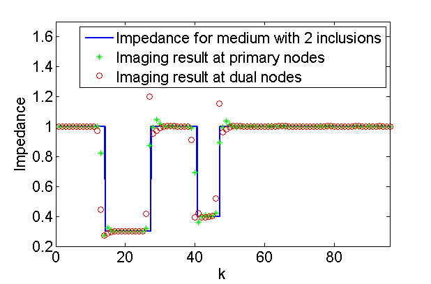
Figure 1. Layered relative acoustic impedance model $\sigma(x)$ and discrete inversion results. The discrete inversion is discussed in section 3.1. The abscissa is the spatial (primary) grid node index, sampled at interval $\tau$.

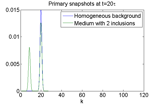
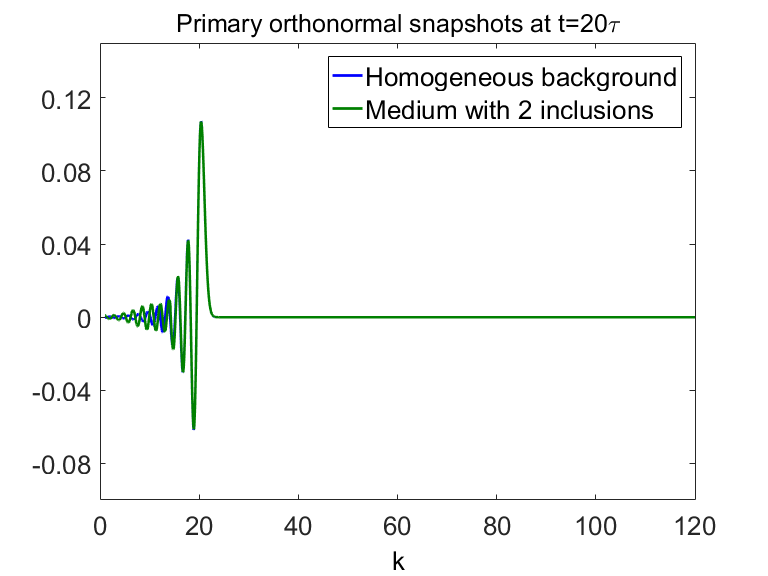
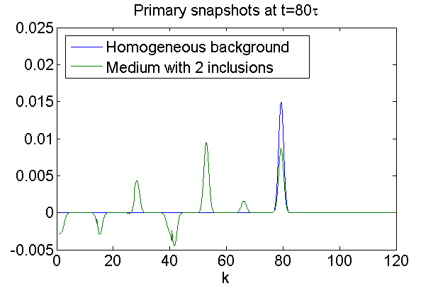
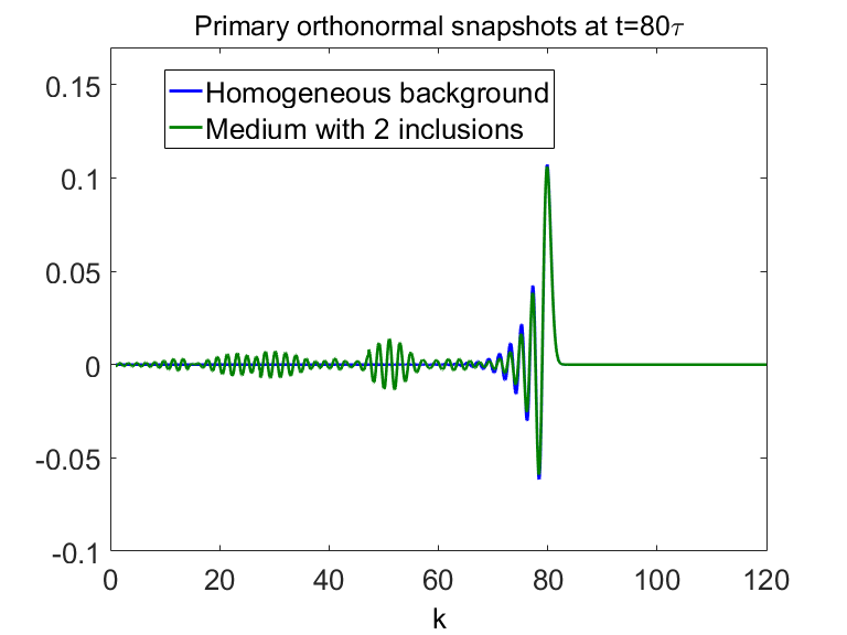
Figure 2. Primary snapshots ${\itbf P}_{j}$ (left column) and primary orthonormal snapshots ${\itbf V}_{j}$ (right column) at time index $j=20$ (top row) and $j=80$ (bottom row). The abscissa is the travel time index, sampled at interval $\tau$.

In Figure 3 we show the raw scattering data, its Born approximation and the data obtained with the DtB algorithm. We observe that the strong multiples in the raw data are removed, and that the result is indistinguishable from the Born approximation.

Remark 2.2.

Our experiments with different $\tau$ (not showed here) indicate that the $l_{\infty}$ discrepancy between the true Born approximation and the output of the DtB algorithm decays as $O(\tau^{2})$ for smooth $\sigma(x)$, in agreement with the approximation error in (59). We speculate that if we solved exactly for ${\itbf L}_{q}$ in (59), the discrepancy would decay exponentially in ${\tau}^{-1}$.

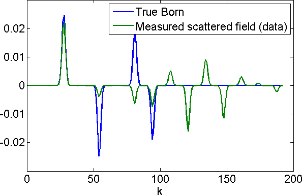
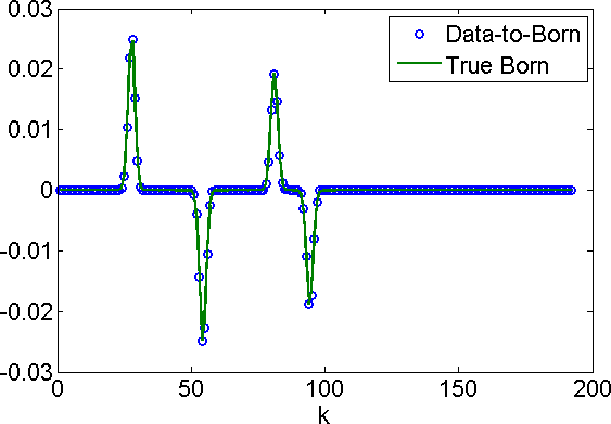
Figure 3. Left: the raw scattering data (green line) and the Born approximation (blue line). Right: the data transformed with the DtB map (blue line) is indistinguishable from the Born approximation (green line). The abscissa is the time index.

3. A related inverse spectral problem

In this section we look in more detail at the entries of the ROM matrix $\widetilde{{\itbf L}}_{q}$, and compare it with another ROM obtained from spectral measurements of the operator (16) in the wave equation.

3.1. The orthonormal snapshots and the entries in $\widetilde{{\itbf L}}_{q}$

The first primary snapshots $\{{\itbf P}_{j}\}_{j=0}^{n-1}$ span the Krylov space $\mathcal{K}_{n}({\itbf b},\boldsymbol{{\mathscr{P}}})$ defined in (70), and the dual snapshots $\{{{\itbf U}}_{j}\}_{j=0}^{n-1}$ span the Krylov space $\mathcal{K}_{n}(\boldsymbol{{U}}_{0},\boldsymbol{\mathscr{U}})$, as follows from definition (64).

The classical method for computing an orthonormal basis of a Krylov subspace is given by the Lanczos method [39], which is used in [20, Algorithm 3.1] to calculate the orthogonal vectors $\{\overline{\bf p}_{j}\}_{j=1}^{n}$ and the orthogonal vectors $\{\overline{\bf u}_{j}\}_{j=1}^{n}$, satisfying the equations

$$\frac{\overline{\bf p}_{j+1}-\overline{\bf p}_{j}}{\gamma_{j}}=-\boldsymbol{\mathcal{L}}_{q}\overline{\bf u}_{j},\quad\frac{\overline{\bf u}_{j}-\overline{\bf u}_{j-1}}{\widehat{\gamma}_{j}}=\boldsymbol{\mathcal{L}}_{q}^{T}\overline{\bf p}_{j},$$ (95)

for $j\geq 1$, with initial conditions $\overline{\bf p}_{1}={\itbf b},$ $\overline{\bf u}_{0}=0,$ and coefficients

$$\gamma_{j}=\frac{1}{\|\overline{\bf u}_{j}\|^{2}},\quad\widehat{\gamma}_{j}=\frac{1}{\|\overline{\bf p}_{j}\|^{2}},\quad j=1,\ldots,n.$$ (96)

It is also shown in [20, Sections 4.2, 4.3] how the coefficients (96) enter the expression of the tridiagonal ROM propagator $\widetilde{\boldsymbol{{\mathscr{P}}}}$. Using the factorization (82), we obtain from those results the lower bidiagonal matrix $\widetilde{{\itbf L}}_{q}$ with entries

$$(\widetilde{{\itbf L}}_{q})_{j,j} =-1/\sqrt{\gamma_{j}\widehat{\gamma}_{j}},\quad j=1,\ldots,n,$$

$$(\widetilde{{\itbf L}}_{q})_{j+1,j} =1/\sqrt{\gamma_{j}\widehat{\gamma}_{j+1}},\quad j=1,\ldots,n-1.$$ (97)

The columns of the projection matrix ${\itbf V}$ on the Krylov space $\mathcal{K}_{n}({\itbf b},\boldsymbol{{\mathscr{P}}})$, aka the orthonormal primary snapshots, are given by

$${\itbf V}_{j}=\sqrt{\widehat{\gamma}_{j}}\,\overline{\bf p}_{j},\quad j=1,\ldots,n,$$ (98)

and the projection matrix ${\itbf W}$ satisfies by definition (88)

$${\itbf W}\widetilde{{\itbf L}}_{q}^{T}=\boldsymbol{\mathcal{L}}_{q}^{T}{\itbf V}.$$ (99)

The $j$-th column in this equation reads

$$\frac{1}{\sqrt{\widehat{\gamma}_{j}}}{\itbf W}\widetilde{{\itbf L}}_{q}^{T}\itbf{e}_{j}=\boldsymbol{\mathcal{L}}_{q}^{T}\overline{\bf p}_{j}=\frac{\overline{\bf u}_{j}-\overline{\bf u}_{j-1}}{\widehat{\gamma}_{j}},$$ (100)

where we used (95) and (98). The left hand side is a linear combination of the columns ${\itbf W}_{j}$ and ${\itbf W}_{j-1}$ of ${\itbf W}$, because $\widetilde{{\itbf L}}_{q}$ is lower bidiagonal. Using the expression (97) of the entries in $\widetilde{{\itbf L}}_{q}$ and equation (98), we conclude that

$${\itbf W}=\Big{(}{\itbf W}_{1},\ldots,{\itbf W}_{n}),\quad{\itbf W}_{j}=\sqrt{\gamma_{j}}\,\overline{\bf u}_{j}.$$ (101)

This shows that ${\itbf W}$ is the matrix of orthormal dual snapshots, as stated in the previous section.

Let us take the constant reference impedance $\sigma^{0}=1$, corresponding to the potential $q^{0}=0$, and define the coefficients

$$\sigma_{j}=\frac{\widehat{\gamma}_{j}^{0}}{\widehat{\gamma}_{j}}=\frac{\|\overline{\bf p}_{j}\|^{2}}{\|\overline{\bf p}^{0}_{j}\|^{2}},\qquad\widehat{\sigma}_{j}=\frac{\gamma_{j}}{\gamma_{j}^{0}}=\frac{\|\overline{\bf u}^{0}_{j}\|^{2}}{\|\overline{\bf u}_{j}\|^{2}}.$$ (102)

With these coefficients we introduce the discrete Liouville transform

$$\overline{{\itbf P}}_{j}=\frac{\overline{\bf p}_{j}}{\sqrt{\sigma_{j}}},\quad\overline{{{\itbf U}}}_{j}=\sqrt{\widehat{\sigma}_{j}}\,\overline{\bf u}_{j},$$ (103)

substitute it in (95) and obtain after straightforward algebraic manipulations the system

$$\frac{\overline{{\itbf P}}_{j+1}-\overline{{\itbf P}}_{j}}{\gamma_{j}^{0}}+\overline{{\itbf P}}_{j+1}\left(\frac{\sqrt{\sigma_{j+1}}-\sqrt{\widehat{\sigma}_{j}}}{\gamma_{j}^{0}\sqrt{\widehat{\sigma}_{j}}}\right)+\overline{{\itbf P}}_{j}\left(\frac{\sqrt{\widehat{\sigma}_{j}}-\sqrt{\sigma_{j}}}{\gamma_{j}^{0}\sqrt{\widehat{\sigma}_{j}}}\right) =-\boldsymbol{\mathcal{L}}_{q}\overline{{{\itbf U}}}_{j},$$ (104)

$$\frac{\overline{{{\itbf U}}}_{j}-\overline{{{\itbf U}}}_{j-1}}{\widehat{\gamma}_{j}^{0}}-\overline{{{\itbf U}}}_{j}\left(\frac{\sqrt{\widehat{\sigma}_{j}}-\sqrt{\sigma_{j}}}{\widehat{\gamma}_{j}^{0}\sqrt{\widehat{\sigma}_{j}}}\right)-\overline{{{\itbf U}}}_{j-1}\left(\frac{\sqrt{\sigma_{j}}-\sqrt{\widehat{\sigma}_{j-1}}}{\widehat{\gamma}_{j}^{0}\sqrt{\widehat{\sigma}_{j-1}}}\right) =\boldsymbol{\mathcal{L}}_{q}^{T}\overline{{\itbf P}}_{j},$$ (105)

for $j=1,\ldots,n$. Recalling the approximation (61), we see that the finite difference operators in the left hand sides of equations (104)-(105) can be interpreted as discretizations of $L_{q}^{T}=\partial_{T}+\frac{1}{2}\partial_{T}q(T)$ and $-L_{q}=\partial_{T}-\frac{1}{2}\partial_{T}q(T)$, with $q(T)=\ln\sigma(T)$. The discretization is on a special grid with primary points spaced at $\gamma_{j}^{0}$, and dual points spaced at $\widehat{\gamma}_{j}^{0}$. In our case these equal $\tau$ [20]. In Figure 2 the primary grid corresponds to the integer values in the abscissa, and the dual grid points are offset by $\tau/2$. We note that the peaks of the primary orthonormal snapshots ${\itbf V}_{j}$ are approximately aligned with the $j$-th primary grid point, which is the location of the wavefront.

The coefficients $\sigma_{j}$ and $\widehat{\sigma}_{j}$ are approximations of the impedance at the primary and dual grid points, and the terms in the parentheses in (104)-(105) are discretizations of

$$\frac{1}{2}\partial_{T}q(T)=\frac{\partial_{T}\sqrt{\sigma(T)}}{\sqrt{\sigma(T)}}.$$

We display in Figure 1 the values $\sigma_{j}$ and $\widehat{\sigma}_{j}$ computed for the impedance model considered in section 2.5. They give a reasonable approximation of the discontinuous impedance, but better results can be obtained by inverting the data processed by the DtB algorithm, which is almost indistinguishable from the Born approximation.

We show next that the same approximation formulas (102) arise for another ROM, constructed from different measurement functions of the operator $L_{q}L_{q}^{T}$ than in (65). The values of the ROM coefficients $\{\gamma_{j},\widehat{\gamma}_{j}\}_{j=1}^{n}$ are different, but the same ratios $\{\widehat{\gamma}_{j}^{0}/\widehat{\gamma}_{j},\gamma_{j}/\gamma_{j}^{0}\}_{j=1}^{n}$ define approximations of $\sigma(T)$ on the ROM dependent grids with primary and dual point spacings defined by $\{\gamma_{j}^{0},\widehat{\gamma}_{j}^{0}\}_{j=1}^{n}$. With this ROM described below, it is proved in [8] that the approximations (102) converge to the unknown impedance function $\sigma(T)$ in the limit $n\to\infty$.

3.2. The spectrally matched ROM

In this section we draw an analogy between the ROM constructed from the data matching conditions (5) and the ”spectrally matched” ROM introduced and analyzed in [8]. Spectrally matched means that the ROM defines a three point finite difference scheme in $x$ for the wave equation satisfied by the pressure field ${p}(t,x)$ in (26), modeled with an $n\times n$ tridiagonal matrix constructed from the truncated spectral measure of the differential operator $A$ in (16).

The Laplace transform of ${p}(t,x)$ with respect to time $t$, written in the travel time coordinates (36),

$$\breve{p}(s,T)=\int_{0}^{\infty}{p}(t,x(T))e^{-st}ds,$$ (106)

satisfies the boundary value problem

$$\big{(}A_{q}+s^{2})\breve{p}(s,T) =s\sqrt{\sigma(T)}b(T)~{}~{}\mbox{for}~{}T\in(0,T_{\ell}),\quad\partial_{T}\breve{p}(s,0)=\breve{p}(s,T_{\ell})=0.$$ (107)

Here we wrote the operator in (16) in the travel time coordinates

$$A_{q}=-\sigma(T)\partial_{T}\Big{(}\frac{1}{\sigma(T)}\partial_{T}\Big{)}=-\partial_{T}^{2}+\partial_{T}q(T)\partial_{T},$$ (108)

with $q(T)=\ln\sigma(T)$. This is the formulation considered in [8], and the spectral measure of $A_{q}$ is defined by its eigenvalues $\{\lambda_{j}>0\}_{j\geq 1}$ and $\{\zeta_{j}=y_{j}^{2}(0)\}_{j\geq 1}$, where $\{y_{j}(T)\}_{j\geq 1}$ are the eigenfunctions, orthonormal with respect to the weighted inner product $\left<\cdot,\cdot\right>_{1/\sigma}$.

The spectrally matched ROM is defined in [8] by an $n\times n$ tridiagonal matrix with spectral measure defined by $\{\lambda_{j},\zeta_{j}\}_{j=1}^{n}$. To compare it with the ROM defined in section 2.3, let us consider the Liouville transform

$$\breve{P}(s,T)=\frac{\breve{p}(s,T)}{\sqrt{\sigma(T)}},$$ (109)

and suppose that $\sigma(T)$ is constant in a vicinity of $T=0$. Then, $\breve{P}(s,T)$ satisfies

$$\big{(}L_{q}L_{q}^{T}+s^{2}\big{)}\breve{P}(s,T) =sb(T)~{}~{}\mbox{for}~{}T\in(0,T_{\ell}),\quad\partial_{T}\breve{P}(s,0)=\breve{P}(s,T_{\ell})=0,$$ (110)

with $L_{q}$ and $L_{q}^{T}$ defined in (37) and (38). Note that $L_{q}L_{q}^{T}$ is related to $A_{q}$ by a similarity transformation,

$$L_{q}L_{q}^{T}=\sigma(T)^{-1/2}A_{q}\sigma(T)^{1/2},$$ (111)

so it has the same eigenvalues $\lambda_{j}$. The eigenfunctions $z_{j}(T)=\sigma(T)^{-1/2}y_{j}(T)$ are orthonormal with respect to the Euclidian $L^{2}\big{(}(0,T_{\ell})\big{)}$ inner product. Thus, the spectral measure of $L_{q}L_{q}^{T}$ is the same as that of $A_{q}$, up to the multiplicative constant $1/\sigma(0)$, which we take equal to $1$.

The measurement functions in the data model (4) are now

$$M_{j}(L_{q}L_{q}^{T})=\left\{\begin{array}[]{ll}\lambda_{j+1},&j=0,\ldots,n-1\\ z^{2}_{j-n+1}(0),&j=n,\ldots 2n-1.\end{array}\right.$$ (112)

The ROM is defined by the $n\times n$ symmetric, positive definite and tridiagonal matrix ${\boldsymbol{\widetilde{\mathcal{A}}}}_{q}$ in the finite difference discretization of (110) on a special grid with $n$ points in $[0,T_{\ell}]$,

$$\big{(}{\boldsymbol{\widetilde{\mathcal{A}}}}_{q}+s^{2}\big{)}\widetilde{{\itbf P}}(s)=s\|b\|{\bf e}_{1}.$$ (113)

Let

$${\boldsymbol{\widetilde{\mathcal{A}}}}_{q}=\widetilde{{\itbf L}}_{q}\widetilde{{\itbf L}}_{q}^{T},$$ (114)

be the Cholesky factorization of this matrix, with lower bidiagonal $\widetilde{{\itbf L}}_{q}$. Let also $\widetilde{\lambda}_{j}$ and $\widetilde{\itbf z}_{j}$ be the eigenvectors of ${\boldsymbol{\widetilde{\mathcal{A}}}}_{q}$, with Euclidean norm $\|\widetilde{\itbf z}_{j}\|=1$. The matrix ${\boldsymbol{\widetilde{\mathcal{A}}}}_{q}$ is obtained from the matching conditions

$$M_{j}(L_{q}L_{q}^{T})=\widetilde{M}_{j}(\widetilde{{\itbf L}}_{q}\widetilde{{\itbf L}}_{q}^{T})=\left\{\begin{array}[]{ll}\widetilde{\lambda}_{j+1},&j=0,\ldots,n-1\\ \big{(}{\bf e}_{1}^{T}\widetilde{\itbf z}_{j}\big{)}^{2},&j=n,\ldots 2n-1,\end{array}\right.$$ (115)

using the Lanczos algorithm [15]. The resulting lower bidiagonal matrix $\widetilde{{\itbf L}}_{q}$ has the entries

$$(\widetilde{{\itbf L}}_{q})_{j,j} =-\frac{1}{\sqrt{\gamma_{j}\widehat{\gamma}_{j}}},\quad 1\leq j\leq n,\quad(\widetilde{{\itbf L}}_{q})_{j+1,j}=\frac{1}{\sqrt{\gamma_{j}\widehat{\gamma}_{j+1}}},\quad 1\leq j\leq n-1,$$ (116)

that have the same expression as in (97), but the values of $\{\gamma_{j},\widehat{\gamma}_{j}\}_{j=1}^{n}$ are different.

3.3. Inversion on the spectrally matched grid

With the factorization (114) we can rewrite (113) as the first order system

$$s\widetilde{\boldsymbol{\it{U}}}(s)=\widetilde{{\itbf L}}_{q}^{T}\widetilde{\itbf P}(s),\quad s\widetilde{\itbf P}(s)=-\widetilde{{\itbf L}}_{q}\widetilde{\boldsymbol{\it{U}}}(s)+\|b\|{\bf e}_{1},$$ (117)

for the ROM primary and dual vectors $\widetilde{\itbf P}(s)$ and $\widetilde{\boldsymbol{\it{U}}}(s)$. We now show that the entries in these vectors represent discretizations of the Laplace transforms $\breve{P}(s,T)$ and $\breve{U}(s,T)$ of the primary and dual fields in equations (30), rewritten in travel time coordinates. The discretization grid is defined by the spectrally matched ROM coefficients $\{\gamma^{0}_{j},\widehat{\gamma}_{j}^{0}\}_{j=1}^{n}$ calculated in the reference medium with constant impedance $\sigma^{0}=1$ i.e., potential $q^{0}=0$. It is proved in [8, Lemma 3.2] that these coefficients define a staggered grid in the interval $[0,T_{\ell}]$,

$$0=\widehat{T}_{0}=T_{1}<\widehat{T}_{1}<T_{2}<\widehat{T}_{2}<\ldots<\widehat{T}_{n}<T_{n+1},$$ (118)

with $T_{n+1}$ approaching $T_{\ell}$ from below in the limit $n\to\infty$. The primary field $\breve{P}(s,T)$ is discretized on the grid with points $\{T_{j}\}_{j=1}^{n+1}$, spaced at intervals $h_{j}=\gamma_{j}^{0}=T_{j+1}-T_{j},$ and the dual field $\breve{U}(s,T)$ is discretized on the grid with points $\{\widehat{T}_{j}\}_{j=0}^{n}$, spaced at intervals $\widehat{h}_{j}=\widehat{\gamma}_{j}^{0}=\widehat{T}_{j}-\widehat{T}_{j-1},$ for $j=1,\ldots,n$.

Let us define the diagonal matrices

$$H^{1/2}=\mbox{diag}\big{(}h_{1}^{1/2},\ldots,h_{n}^{1/2}\big{)},\quad\widehat{H}^{1/2}=\mbox{diag}\big{(}\widehat{h}_{1}^{1/2},\ldots,\widehat{h}_{n}^{1/2}\big{)},$$

and write the vectors in (117) in the form

$$\widetilde{\itbf P}(s)=\widehat{H}^{1/2}\begin{pmatrix}\breve{P}_{{}_{T_{1}}}(s)\\ \vdots\\ \breve{P}_{{}_{T_{n}}}(s)\end{pmatrix},\quad\widetilde{\boldsymbol{\it{U}}}(s)=H^{1/2}\begin{pmatrix}\breve{U}_{{}_{\widehat{T}_{1}}}(s)\\ \vdots\\ \breve{U}_{{}_{\widehat{T}_{n}}}(s)\end{pmatrix},$$ (119)

so that the first equation in the system (117) becomes

$$s\begin{pmatrix}\breve{U}_{{}_{\widehat{T}_{1}}}(s)\\ \vdots\\ \breve{U}_{{}_{\widehat{T}_{n}}}(s)\end{pmatrix} =H^{-1/2}\widetilde{{\itbf L}}_{q}^{T}\widehat{H}^{1/2}\begin{pmatrix}\breve{P}_{{}_{T_{1}}}(s)\\ \vdots\\ \breve{P}_{{}_{T_{n}}}(s)\end{pmatrix}.$$ (120)

Let also

$$\sigma_{j}=\frac{\widehat{h}_{j}}{\widehat{\gamma}_{j}}=\frac{\widehat{\gamma}_{j}^{0}}{\widehat{\gamma}_{j}},\quad\widehat{\sigma}_{j}=\frac{\gamma_{j}}{h_{j}}=\frac{\gamma_{j}}{\gamma_{j}^{0}},\quad j=1,\ldots,n,$$ (121)

and write explicitly the $j$-th equation in (120)

$$s\,\breve{U}_{{}_{\widehat{T}_{j}}}(s)=\frac{\breve{P}_{{}_{T_{j+1}}}(s)-\breve{P}_{{}_{T_{j}}}(s)}{h_{j}}+\breve{P}_{{}_{T_{j+1}}}(s)\left(\frac{\sqrt{\sigma_{j+1}}-\sqrt{\widehat{\sigma}_{j}}}{h_{j}\sqrt{\widehat{\sigma}_{j}}}\right)+\breve{P}_{{}_{T_{j}}}(s)\left(\frac{\sqrt{\widehat{\sigma}_{j}}-\sqrt{\sigma_{j}}}{h_{j}\sqrt{\widehat{\sigma}_{j}}}\right).$$

This is the discretization of equation

$$s\breve{U}(s,T)=L_{q}^{T}\breve{P}(s,T)=\partial_{T}\breve{P}(s,T)+\partial_{T}\ln\sqrt{\sigma(T)}\breve{P}(s,T),$$

on the spectrally matched grid. A similar result applies to the second equation in (117), which is the discretization of

$$s\breve{P}(s,T)=-L_{q}\breve{U}(s,T)+b(T).$$

The ratios (121) are of the same form as in (102) and represent approximations of the impedance function $\sigma(T)$ on the spectrally matched grid (118). Specifically, it is proved in [8, Theorem 6.1] that if $\sigma(T)$ is smooth, then the piecewise constant function

$$\sigma^{n}(T)=\left\{\begin{array}[]{ll}\sigma_{j}&\mbox{for}~{}T\in[T_{j},\widehat{T}_{j}),~{}j=1,\ldots,n,\\ \widehat{\sigma}_{j}&\mbox{for}~{}T\in[\widehat{T}_{j},T_{j+1}),~{}j=1,\ldots,n,\\ \widehat{\sigma}_{n}&\mbox{for}~{}T\in[T_{n+1},T_{\ell}],\end{array}\right.$$

converges to $\sigma(T)$ pointwise and in $L^{1}[0,T_{\ell}]$, as $n\to\infty$.

4. The multi dimensional case

In this section we generalize the DtB mapping from one dimension, as described in section 2, to $\mathbb{R}^{d}$ with $d>1$. The derivation follows the same strategy as in section 2, with certain modifications described below.

4.1. Data model for an array of sensors

In the multi-dimensional case we consider an array of $m$ sensors on the accessible boundary $\partial\Omega_{a}$, located at points ${{\itbf x}}_{s}\in\partial\Omega_{a}$, for $s=1,\ldots,m$. Each sensor excites a pressure field, the solution of the wave equation

$$\big{(}\partial_{t}^{2}+A\big{)}\mathfrak{p}_{s}(t,{{\itbf x}})=\partial_{t}f(t)\delta({{\itbf x}}-{{\itbf x}}_{s}),\quad-\infty<t<\infty,~{}~{}{{\itbf x}}\in\Omega,$$ (122)

where the index $s$ denotes the source and the operator $A$ is now defined as

$$A=-\sigma({{\itbf x}})c({{\itbf x}})\nabla\cdot\Big{[}\frac{c({{\itbf x}})}{\sigma({{\itbf x}})}\nabla\Big{]},$$ (123)

with $\nabla$ denoting the gradient and $\nabla\cdot$ the divergence operator. For simplicity, we assume that the same pulse $\partial_{t}f(t)$ is emitted from all the sensors. The boundary conditions at $\partial\Omega_{a}$ are $\nabla\mathfrak{p}_{s}(t,{{\itbf x}})\cdot{\boldsymbol{\nu}}({{\itbf x}})=0,$ where ${\boldsymbol{\nu}}({{\itbf x}})$ is the outer unit normal, and on the inaccessible boundary $\partial\Omega_{i}$ we let $\mathfrak{p}_{s}(t,{{\itbf x}})=0.$ The medium is at rest initially, so we set $\mathfrak{p}_{s}(t,{{\itbf x}})=0,$ for $t\ll 0.$

Following the same argument that lead to equation (22), we define the matrix-valued data ${\itbf D}_{k}\in\mathbb{R}^{m\times m}$ with entries defined by

$$({\itbf D}_{k})_{i,j}=\mathfrak{p}_{i}(t_{k},{{\itbf x}}_{j})+\mathfrak{p}_{i}(-t_{k},{{\itbf x}}_{j}),\quad i,j=1,\ldots,m,$$ (124)

in terms of the measurements at the instances $t_{k}=k\tau$ for $k=0,1,\ldots,2n-1$. For each $k$ the matrix ${\itbf D}_{k}$ is symmetric due to the source-receiver reciprocity.

4.2. First order system form and Liouville transformation

Similar to the one-dimensional case, we introduce the sensor functions

$$b_{s}({{\itbf x}})=\sqrt{\frac{\sigma({{\itbf x}}_{s})c({{\itbf x}}_{s})}{\sigma({{\itbf x}})}}[\widehat{f}(\sqrt{A})]^{1/2}\delta({{\itbf x}}-{{\itbf x}}_{s}),\quad{{\itbf x}}\in\Omega,\quad s=1,\ldots,m,$$ (125)

and define the analogue of (25)

$${p}_{s}(t,{{\itbf x}})=\cos(t\sqrt{A})\sqrt{\sigma({{\itbf x}})}b_{s}({{\itbf x}}),\quad s=1,\ldots,m.$$ (126)

Here $p_{s}(t,{{\itbf x}})$ is the pressure field in the first order system

$$\partial_{t}\begin{pmatrix}{p}_{s}(t,{{\itbf x}})\\ -{\itbf u}_{s}(t,{{\itbf x}})\end{pmatrix}=\begin{pmatrix}0&\sigma({{\itbf x}})c({{\itbf x}})\nabla\cdot\\ \frac{c({{\itbf x}})}{\sigma({{\itbf x}})}\nabla&0\end{pmatrix}\begin{pmatrix}{p}_{s}(t,{{\itbf x}})\\ -{\itbf u}_{s}(t,{{\itbf x}})\end{pmatrix},\quad t>0,\quad{{\itbf x}}\in\Omega,$$ (127)

with initial conditions

$${p}_{s}(0,{{\itbf x}})=\sqrt{\sigma({{\itbf x}})}{\it{b}}_{s}({{\itbf x}})\quad\mbox{and}\quad{\itbf u}_{s}(0,{{\itbf x}})=0,\qquad{{\itbf x}}\in\Omega,$$ (128)

and boundary conditions

$${p}_{s}(t,{{\itbf x}})|_{{{\itbf x}}\in\Omega_{i}}=0\quad\mbox{and}\quad{\itbf u}_{s}(t,{{\itbf x}})|_{{{\itbf x}}\in\Omega_{a}}=0,\qquad t>0.$$ (129)

This system is the analogue of (26) and the vector field ${\itbf u}_{s}(t,{{\itbf x}})$ is the particle velocity.

Using the Liouville transformation

$${\it{P}}(t,{{\itbf x}};{{\itbf x}}_{s})=\frac{p(t,{{\itbf x}};{{\itbf x}}_{s})}{\sqrt{\sigma({{\itbf x}})}},\quad{\boldsymbol{\it{U}}}(t,{{\itbf x}};{{\itbf x}}_{s})=-\sqrt{\sigma({{\itbf x}})}{\itbf u}(t,{{\itbf x}};{{\itbf x}}_{s}),$$ (130)

we rewrite (127) as a Schrödinger system (1) with the operators $L_{q}$ and $L_{q}^{T}$ given by

$$L_{q}=-c({{\itbf x}})\nabla\cdot\;+\frac{1}{2}c({{\itbf x}})\nabla q({{\itbf x}})\cdot~{}~{}\mbox{and}~{}~{}L_{q}^{T} =c({{\itbf x}})\nabla+\frac{1}{2}c({{\itbf x}})\nabla q({{\itbf x}}),$$ (131)

and the same $q({{\itbf x}})=\ln\sigma({{\itbf x}})$. The transformed boundary and initial conditions take the form (2)–(3), and the entries of the data matrix ${\itbf D}_{k}\in\mathbb{R}^{m\times m}$, for $k=0,\ldots,2n-1$, are expressed in terms of the primary wave ${\it{P}}_{i}(t,{{\itbf x}})$ as

$$({\itbf D}_{k})_{i,j}=\left<b_{j},{\it{P}}_{i}(t_{k},\cdot)\right>_{\frac{1}{c({{\itbf x}})}}=\int_{\Omega}\frac{d{{\itbf x}}}{c({{\itbf x}})}{\it{b}}_{j}({{\itbf x}}){\it{P}}_{i}(t_{k},{{\itbf x}}),\quad i,j=1,\ldots,m.$$ (132)

4.3. Symmetrized data model, propagator and measurement function

In one dimension we used travel time coordinates to write the data model in the symmetrized form. Because such a transformation is not available in higher dimensions, we follow a different approach to symmetrize (132) and thus obtain an analogue of (44).

Combining (132) with (126) and (130) we write

$$({\itbf D}_{k})_{i,j}=\int_{\Omega}\frac{d{{\itbf x}}}{c({{\itbf x}})}b_{j}({{\itbf x}})\sigma^{-1/2}({{\itbf x}})\cos(t_{k}\sqrt{A})\sigma^{1/2}({{\itbf x}})b_{i}({{\itbf x}}),$$ (133)

where we assume for the remainder of this section $i,j=1,\ldots,m$, and $k=0,\ldots,2n-1$. From the definition (131) of $L_{q}$ it follows that

$$A=\sigma^{1/2}({{\itbf x}})L_{q}L_{q}^{T}\sigma^{-1/2}({{\itbf x}}).$$ (134)

Hence,

$$({\itbf D}_{k})_{i,j}=\int_{\Omega}\frac{d{{\itbf x}}}{c({{\itbf x}})}b_{j}({{\itbf x}})\cos\Big{(}t_{k}\sqrt{L_{q}L_{q}^{T}}\Big{)}b_{i}({{\itbf x}}),$$ (135)

where we used that analytic matrix functions commute with similarity transformations. We use another similarity transformation to rewrite (135) as

$$({\itbf D}_{k})_{i,j}=\int_{\Omega}d{{\itbf x}}\;b_{j}^{c}({{\itbf x}})\cos\Big{(}t_{k}\sqrt{c^{-1/2}L_{q}L_{q}^{T}c^{1/2}}\Big{)}b_{i}^{c}({{\itbf x}}),$$ (136)

with the rescaled sensor functions

$$b^{c}_{s}({{\itbf x}})=c^{-1/2}({{\itbf x}})b_{s}({{\itbf x}}),\quad s=1,\ldots,m.$$ (137)

We also define the rescaled operators

$$L_{q}^{c} =c^{-1/2}({{\itbf x}})L_{q}c^{1/2}({{\itbf x}})=c^{1/2}({{\itbf x}})\left(-\nabla\cdot+\frac{1}{2}\nabla q({{\itbf x}})\;\cdot\right)c^{1/2}({{\itbf x}}),$$ (138)

$$L_{q}^{c^{T}} =c^{-1/2}({{\itbf x}})L_{q}^{T}c^{1/2}({{\itbf x}})=c^{1/2}({{\itbf x}})\left(\nabla+\frac{1}{2}\nabla q({{\itbf x}})\right)c^{1/2}({{\itbf x}}),$$ (139)

which are adjoint to each other with respect to the standard $L^{2}(\Omega)$ inner product. These operators define the propagator for the multi-dimensional problem as in (42),

$${\mathscr{P}}=\cos\Big{(}\tau\sqrt{L_{q}^{c}L_{q}^{c^{T}}}\Big{)}.$$ (140)

The data model (136) is now in symmetric form, and the measurement functions ${\itbf M}_{k}(L_{q}L_{q}^{T})\in\mathbb{R}^{m\times m}$ are defined component-wise by

$$({\itbf D}_{k})_{i,j}=[{\itbf M}_{k}(L_{q}^{c}L_{q}^{c^{T}})]_{i,j}=\left<b_{j}^{c}({{\itbf x}}),\mathcal{T}_{k}({\mathscr{P}})b_{i}^{c}({{\itbf x}})\right>.$$ (141)

Similar to the one-dimensional case, the propagator ${\mathscr{P}}$ can be used to define an exact time stepping scheme for

$${\it{P}}_{k,s}({{\itbf x}})=\mathcal{T}_{k}({\mathscr{P}}){\it{b}}_{s}^{c}({{\itbf x}}),\quad k=0,\ldots,2n-1,\quad s=1,\ldots,m.$$ (142)

Here we use the convention that the first index denotes the discrete time instance and the second index denotes the source. We obtain the same second-order time stepping scheme (48),

$$\frac{1}{\tau^{2}}\Big{[}{\it{P}}_{k+1,s}({{\itbf x}})-2{\it{P}}_{k,s}({{\itbf x}})+{\it{P}}_{k-1,s}({{\itbf x}})\Big{]}=-\xi({\mathscr{P}}){\it{P}}_{k,s}({{\itbf x}}),\quad k=0,\ldots,2n-1,$$ (143)

with the affine function $\xi$ given by (50) and the initial conditions

$${\it{P}}_{0,s}({{\itbf x}})={\it{b}}^{c}_{s}({{\itbf x}}),\quad{\it{P}}_{-1,s}({{\itbf x}})={\it{P}}_{1,s}({{\itbf x}})={\mathscr{P}}{\it{b}}^{c}_{s}({{\itbf x}}).$$ (144)

We also have the same factorization (54) of $\xi({\mathscr{P}})$ in terms of the operator $\mathcal{L}_{q}$ defined as in (56), with $L_{q}$ and $L_{q}^{T}$ replaced by $L_{q}^{c}$ and $L_{q}^{c^{T}}$.

4.4. Multi-input, multi-output reduced order model

The main difference between one and multi dimensions is the type of ROM that we use. In one dimension we had a single-input, single output (SISO) projection ROM (79), obtained from matching the ROM output (85) to the scalar valued data (67). In multi dimensions we need a multi-input, multi-output (MIMO) ROM that matches the matrix valued data (141).

As in section 2.3, let us introduce the matrix ${\itbf A}\in\mathbb{R}^{N\times N}$, a discretization of the operator (123) on a very fine, uniform grid with a total of $N$ nodes and step size $h$. Note that the operator (123) is related to the Schrödinger operators (138)–(139) as

$$A=\sigma^{1/2}({{\itbf x}})L_{q}L_{q}^{T}\sigma^{-1/2}({{\itbf x}})=[\sigma({{\itbf x}})c({{\itbf x}})]^{1/2}L_{q}^{c}L_{q}^{c^{T}}[\sigma({{\itbf x}})c({{\itbf x}})]^{-1/2}.$$ (145)

Let $\boldsymbol{\Sigma}\in\mathbb{R}^{N\times N}$ and ${\itbf C}\in\mathbb{R}^{N\times N}$ be the diagonal matrices with entries given by $\sigma({{\itbf x}})$ and $c({{\itbf x}})$ evaluated at the fine grid nodes. Then we can set ${\itbf L}_{q}$, a fine grid approximation of $L_{q}^{c}$, to be a Cholesky factor of

$${\boldsymbol{\Sigma}}^{-1/2}{\itbf C}^{-1/2}{\itbf A}{\boldsymbol{\Sigma}}^{1/2}{\itbf C}^{1/2}={\itbf L}_{q}{\itbf L}_{q}^{T},$$ (146)

where we drop the index $c$ on ${\itbf L}_{q}$ to simplify notation. We assume as in one dimension that the discretized propagator $\boldsymbol{{\mathscr{P}}}\in\mathbb{R}^{N\times N}$ is well approximated by (62) on the fine grid.

As in one dimension, we call the fine grid discretization of the field $P$ at the measurement instances ”the primary snapshots”. It is convenient to arrange these into matrices ${\itbf P}_{k}\in\mathbb{R}^{N\times m}$, for $k=0,\ldots,2n-1$, with each column corresponding to a different sensor. These matrices satisfy a fine grid analogue of the time stepping scheme (143),

$$\frac{1}{\tau^{2}}\big{(}{\itbf P}_{k+1}-2{\itbf P}_{k}+{\itbf P}_{k-1}\big{)}=-\xi(\boldsymbol{{\mathscr{P}}}){\itbf P}_{k},\quad k=0,\ldots,2n-1,$$ (147)

with initial conditions ${\itbf P}_{0}={\itbf b}$ and ${\itbf P}_{-1}={\itbf P}_{1}=\boldsymbol{{\mathscr{P}}}{\itbf b}.$ The sensor matrix ${\itbf b}\in\mathbb{R}^{N\times m}$ is

$${\itbf b}=[{\itbf b}_{1},\ldots,{\itbf b}_{m}],$$ (148)

where the entries of each column ${\itbf b}_{s}\in\mathbb{R}^{N}$ are the values of the rescaled sensor function $b_{s}^{c}({{\itbf x}})$ evaluated on the fine grid, multiplied by $h^{d/2}$.

The discretized data model and the measurement functions are given by

$${\itbf D}_{k}={\itbf M}_{k}(L_{q}L_{q}^{T})\approx{\itbf M}_{k}({\itbf L}_{q}{\itbf L}_{q}^{T})={\itbf b}^{T}{\itbf P}_{k}={\itbf b}^{T}\mathcal{T}_{k}(\boldsymbol{{\mathscr{P}}}){\itbf b}\in\mathbb{R}^{m\times m},$$ (149)

for $k=0,\ldots,2n-1$. The analogue of equation (66), which relates the data ${\itbf D}_{0}$ at the first time instant to the sensor matrix is

$${\itbf D}_{0}=\begin{bmatrix}\left<b^{c}_{1}({{\itbf x}}),b^{c}_{1}({{\itbf x}})\right>&\left<b^{c}_{1}({{\itbf x}}),b^{c}_{2}({{\itbf x}})\right>&\ldots&\left<b^{c}_{1}({{\itbf x}}),b^{c}_{m}({{\itbf x}})\right>\\ \vdots&\vdots&\ddots&\vdots\\ \left<b^{c}_{m}({{\itbf x}}),b^{c}_{1}({{\itbf x}})\right>&\left<b^{c}_{m}({{\itbf x}}),b^{c}_{2}({{\itbf x}})\right>&\ldots&\left<b^{c}_{m}({{\itbf x}}),b^{c}_{m}({{\itbf x}})\right>\end{bmatrix}\approx{\itbf b}^{T}{\itbf b}.$$ (150)

As we did in one dimension, we neglect henceforth the fine grid discretization errors and treat the approximate relations (149)–(150) as equalities.

The MIMO ROM consists of the symmetric matrix $\widetilde{\boldsymbol{{\mathscr{P}}}}\in\mathbb{R}^{nm\times nm}$, called the ROM propagator, and the ROM sensor matrix $\widetilde{\itbf b}\in\mathbb{R}^{nm\times m}$, satisfying the data matching conditions

$${\itbf D}_{k}=\widetilde{\itbf b}^{T}\mathcal{T}_{k}(\widetilde{\boldsymbol{{\mathscr{P}}}})\widetilde{\itbf b},\quad k=0,\ldots,2n-1.$$ (151)

The matrix $\widetilde{\boldsymbol{{\mathscr{P}}}}$ is block tridiagonal, with $m\times m$ blocks, while $\widetilde{\itbf b}$ has all zeros except for the uppermost $m\times m$ block. Using the $m\times m$ identity matrix ${\itbf I}_{m}$ and zero matrix $\boldsymbol{0}_{m}$, we write

$$\widetilde{\itbf b}={\itbf E}_{1}({\itbf D}_{0})^{1/2},~{}~{}\mbox{with}~{}~{}{\itbf E}_{1}=\begin{bmatrix}{\itbf I}_{m}\\ {\boldsymbol{0}}_{m}\\ \vdots\\ {\boldsymbol{0}}_{m}\end{bmatrix}\in\mathbb{R}^{nm\times m}.$$ (152)

4.5. Calculation of the projection MIMO ROM

The MIMO ROM satisfying the data matching conditions (151) is given by the orthogonal projection of $\boldsymbol{{\mathscr{P}}}$ on the block Krylov subspace, spanned by the columns of

$$\boldsymbol{{P}}=[{\itbf P}_{0},\ldots,{\itbf P}_{n-1}]\in\mathbb{R}^{N\times nm}.$$

We follow the notation in section 2.3.1, and let ${\itbf V}=[{\itbf V}_{1},\ldots,{\itbf V}_{n}]$ be the matrix containing the orthonormal basis for $\mbox{range}(\boldsymbol{{P}})$. Here ${\itbf V}\in\mathbb{R}^{N\times nm}$ and each ${\itbf V}_{k}$ is an $N\times m$ matrix.

To compute the matrices $\boldsymbol{{P}}^{T}\boldsymbol{{P}}$ and $\boldsymbol{{P}}^{T}\boldsymbol{{\mathscr{P}}}\boldsymbol{{P}}$ from the data we can still use the formulas (76) and (81), however, the indexing is understood block-wise. Thus, when we write

$$\big{(}\boldsymbol{{P}}^{T}\boldsymbol{{P}}\big{)}_{i,j} =\frac{1}{2}\Big{(}{\itbf D}_{i+j-2}+{\itbf D}_{|i-j|}\Big{)}\in\mathbb{R}^{m\times m},$$ (153)

$$(\boldsymbol{{P}}^{T}\boldsymbol{{\mathscr{P}}}\boldsymbol{{P}})_{i,j} =\frac{1}{4}\Big{(}{\itbf D}_{i+j-1}+{\itbf D}_{|j-i+1|}+{\itbf D}_{|j-i-1|}+{\itbf D}_{|j+i-3|}\Big{)}\in\mathbb{R}^{m\times m},$$ (154)

for $i,j=1,\ldots,n$, we use the notation $\big{(}\boldsymbol{{P}}^{T}\boldsymbol{{P}}\big{)}_{i,j}$ for the $m\times m$ block of $\boldsymbol{{P}}^{T}\boldsymbol{{P}}\in\mathbb{R}^{nm\times nm}$, at the intersection of rows $(i-1)m+1,\ldots,im$ and columns $(j-1)m+1,\ldots,jm$. We use this notation for $\boldsymbol{{P}}^{T}\boldsymbol{{\mathscr{P}}}\boldsymbol{{P}}\in\mathbb{R}^{nm\times nm}$ and all other block matrices with block size $m\times m$.

Note that (153)–(154) give that $\boldsymbol{{P}}^{T}\boldsymbol{{P}}$ and $\boldsymbol{{P}}^{T}\boldsymbol{{\mathscr{P}}}\boldsymbol{{P}}$ and their blocks are symmetric.

4.6. The Data to Born map

The main difference in the calculation of the DtB mapping is that the Cholesky factorizations (77) and (82) at step 1 of Algorithm 2.1 are replaced with their block Cholesky counterparts given below.

Algorithm 4.1 (Block Cholesky factorization).

Input: the symmetric block matrix ${\itbf X}\in\mathbb{R}^{nm\times nm}$ with $m\times m$ blocks.

To obtain the block Cholesky factorization of ${\itbf X}$ perform the following steps:

$$\mbox{For}~{}k=0,1,\ldots,n-1~{}\mbox{compute:}~{}{\itbf R}_{k,k}={\itbf Q}_{k}\Big{(}{\itbf X}_{k,k}-\sum_{i=0}^{k-1}{\itbf R}_{i,k}^{T}{\itbf R}_{i,k}\Big{)}^{1/2},$$ (155)

where ${\itbf Q}_{k}\in\mathbb{R}^{m\times m}$ is an arbitrary orthogonal matrix.

$$\mbox{For}~{}j=k+1,\ldots,n-1~{}\mbox{compute:}~{}{\itbf R}_{k,j}={\itbf R}_{k,k}^{-1}\Big{(}{\itbf X}_{k,j}-\sum_{i=0}^{k-1}{\itbf R}_{i,k}^{T}{\itbf R}_{i,j}\Big{)}.$$ (156)

Output: the block matrix ${\itbf R}\in\mathbb{R}^{nm\times nm}$ with $m\times m$ blocks, satisfying ${\itbf X}={\itbf R}^{T}{\itbf R}$.

While the regular Cholesky factorization is defined uniquely (assuming it uses the principal value of the square root), there is an ambiguity in defining the block Cholesky factorization, which comes from the computation of the diagonal blocks ${\itbf R}_{k,k}$ in (155). An optimal choice of this matrix is still an open question. We obtained good results with ${\itbf Q}_{k}={\itbf I}$, but here we present another choice (yielding equally good numerical results). This choice allows us to extend the Galerkin-Petrov reasoning of Section 2.4 to the MIMO case. Explicitly, we choose the factor ${\itbf Q}_{k}$ consistent with the MIMO analogue of recursion (95)–(97) for computing the primary and dual orthogonalized block snapshots $\overline{\bf p}_{j}\in\mathbb{R}^{N\times m}$ and $\overline{\bf u}_{j}\in\mathbb{R}^{N\times m}$, for $j=1,\ldots,n.$ Here the coefficients are no longer scalar, but symmetric positive definite matrices ${\boldsymbol{\gamma}}_{j}\in\mathbb{R}^{m\times m}$ and ${\widehat{\boldsymbol{\gamma}}}_{j}\in\mathbb{R}^{m\times m}$. These matrices give the estimates of $\sigma({{\itbf x}})$ in the multidimensional case [20, Section 7.3], so we can extend the reasoning of section 3 to the MIMO case, relating the block-bidiagonal $\widetilde{{\itbf L}}_{q}$ to a discretization of the Schrodinger equation, via the solution of the discrete inverse problem. We describe the computation of the block-bidiagonal $\widetilde{{\itbf L}}_{q}$ in Appendix B.

After the factor $\widetilde{{\itbf L}}_{q}$ is found, the DtB map is computed using the block versions of Algorithms 2.1 and 2.2, with ${\itbf b}$ given by (148) and ${\bf e}_{1}$ replaced by ${\itbf E}_{1}$ from (152). We can also rewrite the MIMO counterpart of (87) in block form. The validity of the MIMO DtB map is based on the assumption of weak dependence of the primary and dual block-QR orthonormal snapshots ${\itbf V}$ and ${\itbf W}$ on $q=\ln\sigma$. Because of the consistency with the discrete inverse problem discussed above, this weak dependence can be understood using the same reasoning as in the SISO case. In particular, similar to the SISO case, the orthonormal snapshots approximate columns of the identity, as shown in Figure 5. We also refer for more details to [22].

Remark 4.1.

Unlike in the one dimensional case, in multi dimensions the DtB algorithm becomes mildly ill-posed, even for the space-time sampling close to the Nyquist rate. A simple regularization algorithm presented in [22] makes the DtB mapping practically insensitive to a reasonable (order of few per cent) level of noise in the measured data for the problem sizes considered in the numerical simulations shown in the next section.

4.7. Numerical results

We begin with numerical results for a two dimensional impedance model with two inclusions and a linear velocity model, shown in Figure 4. We display the relative impedance and wave speed, normalized by their constant values at the sensors. Both the time sampling $\tau$ and the distances between the $m=50$ sensors in the array are chosen close to the Nyquist sampling rate for the Gaussian pulse used in the experiments. As in the one dimensional case, the scattering data and the true Born approximation are computed using a fine grid finite difference time domain scheme, with grid steps much smaller than $\tau$.

$\sigma({{\itbf x}})$	$c({{\itbf x}})$

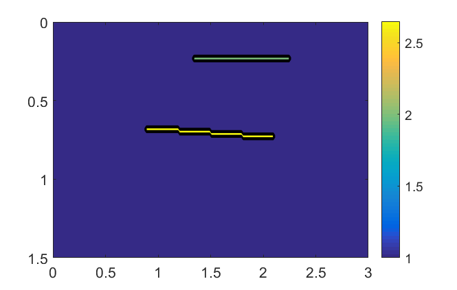
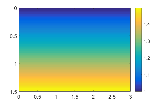
Figure 4. Model $\sigma({{\itbf x}})$ with two inclusions (left) and linear $c({{\itbf x}})$ (right). The axes are in km units.

Columns of $\boldsymbol{{P}}^{0}$	Columns of $\boldsymbol{{P}}$	Columns of ${\itbf V}^{0}$	Columns of ${\itbf V}$

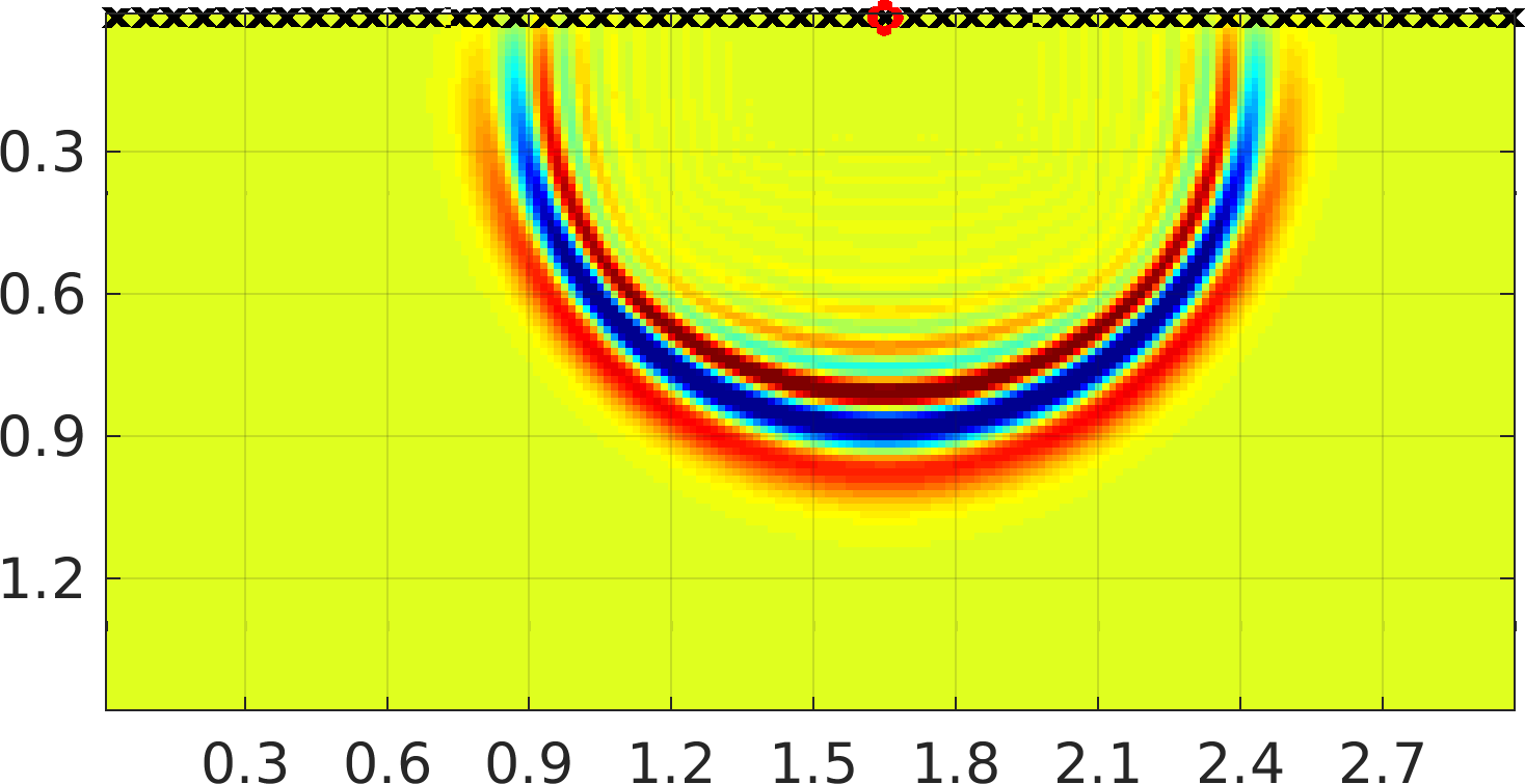
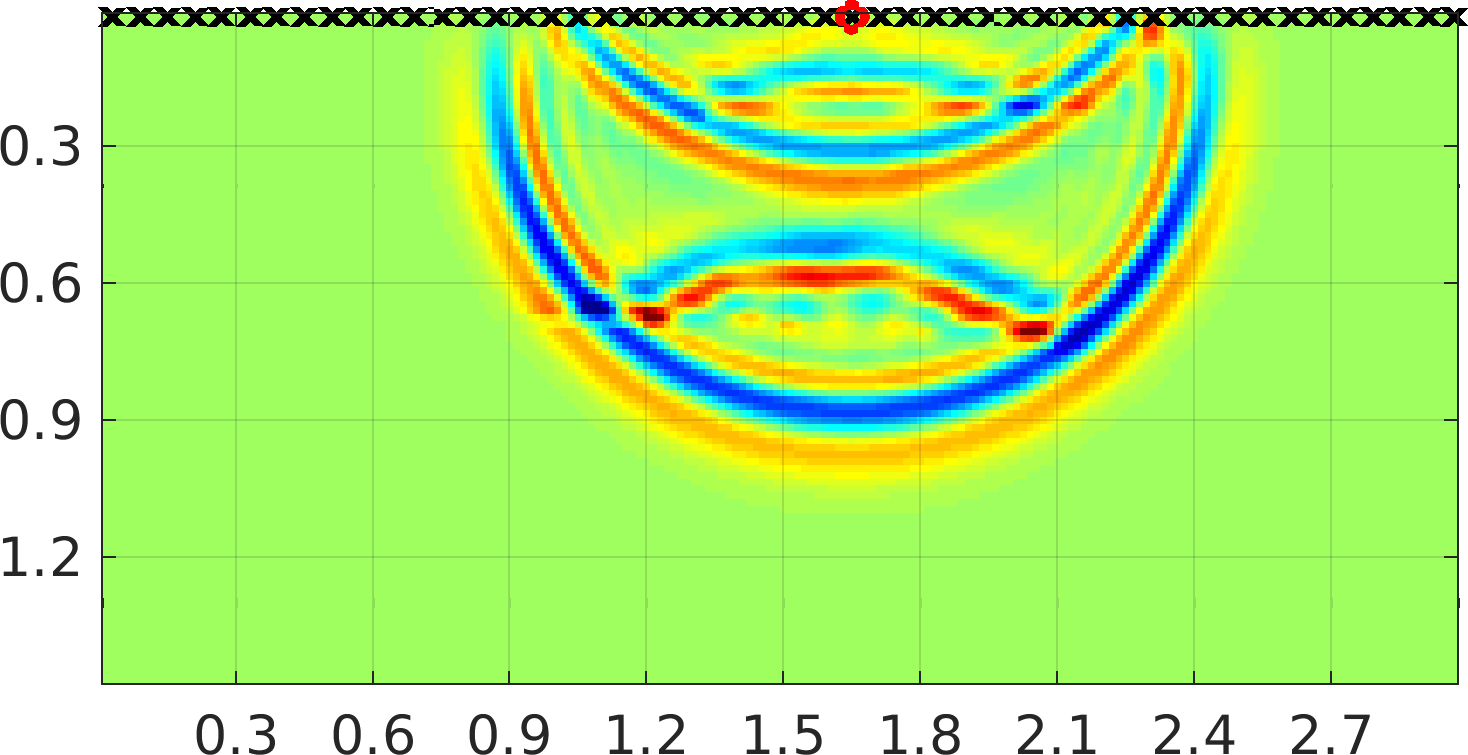
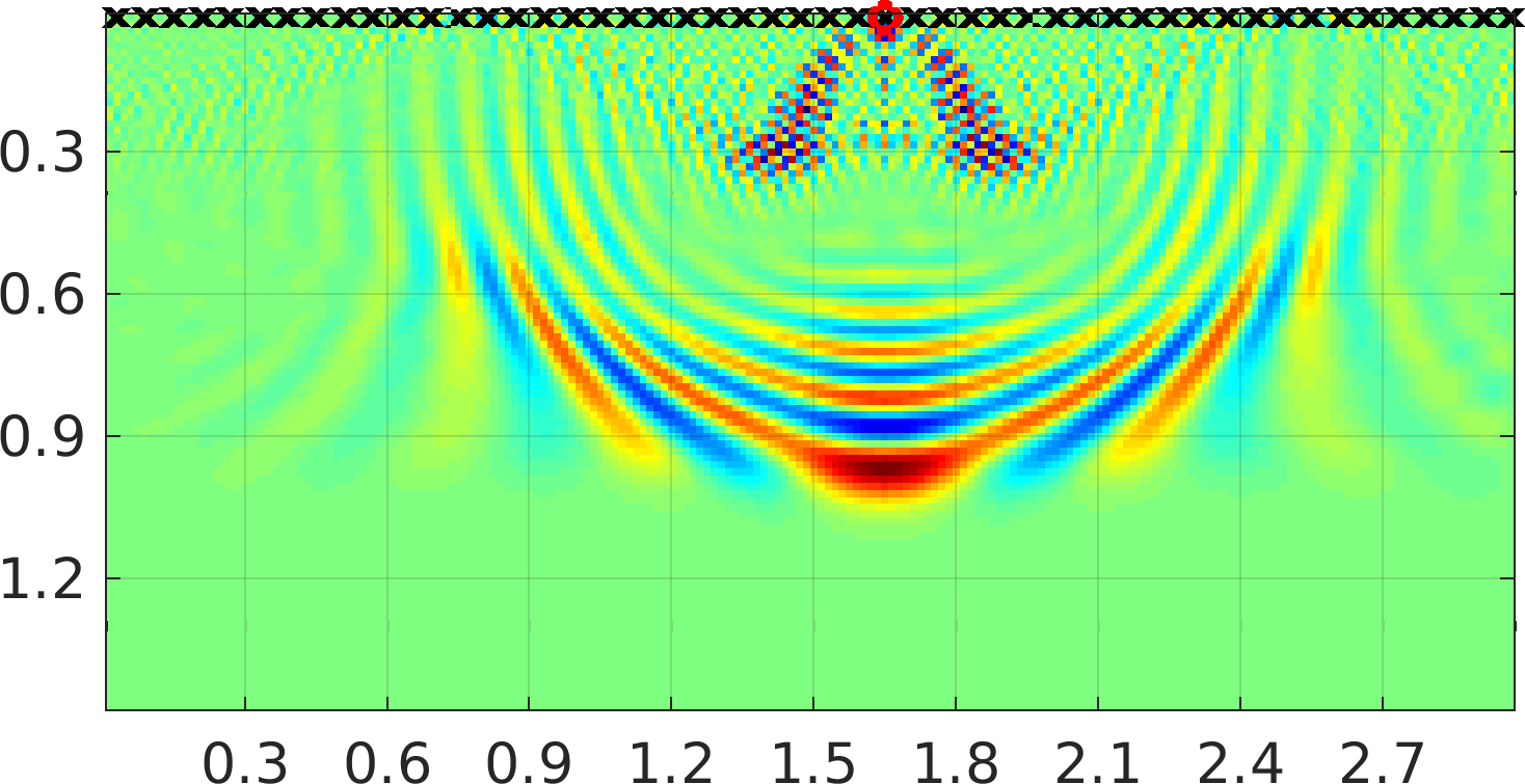
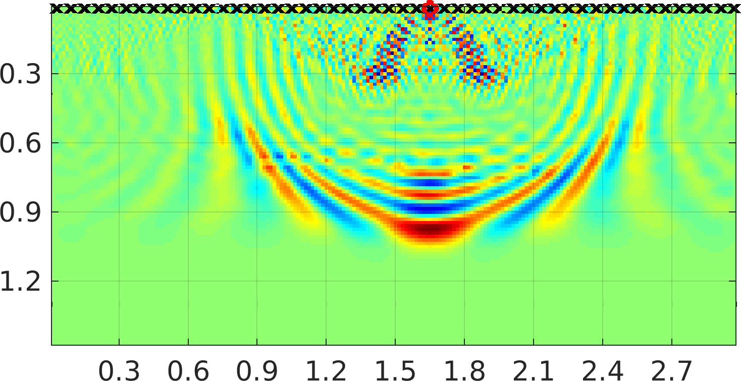
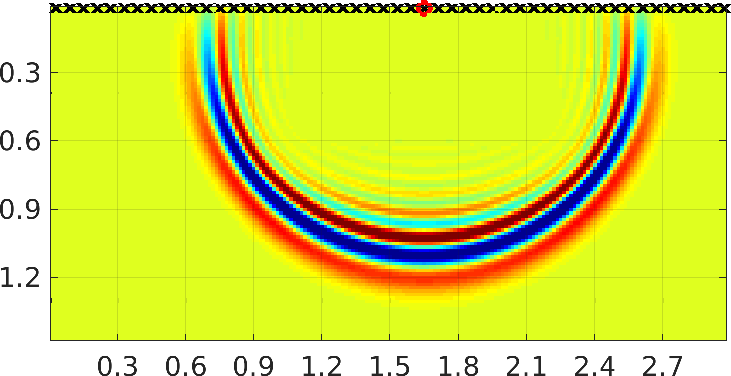
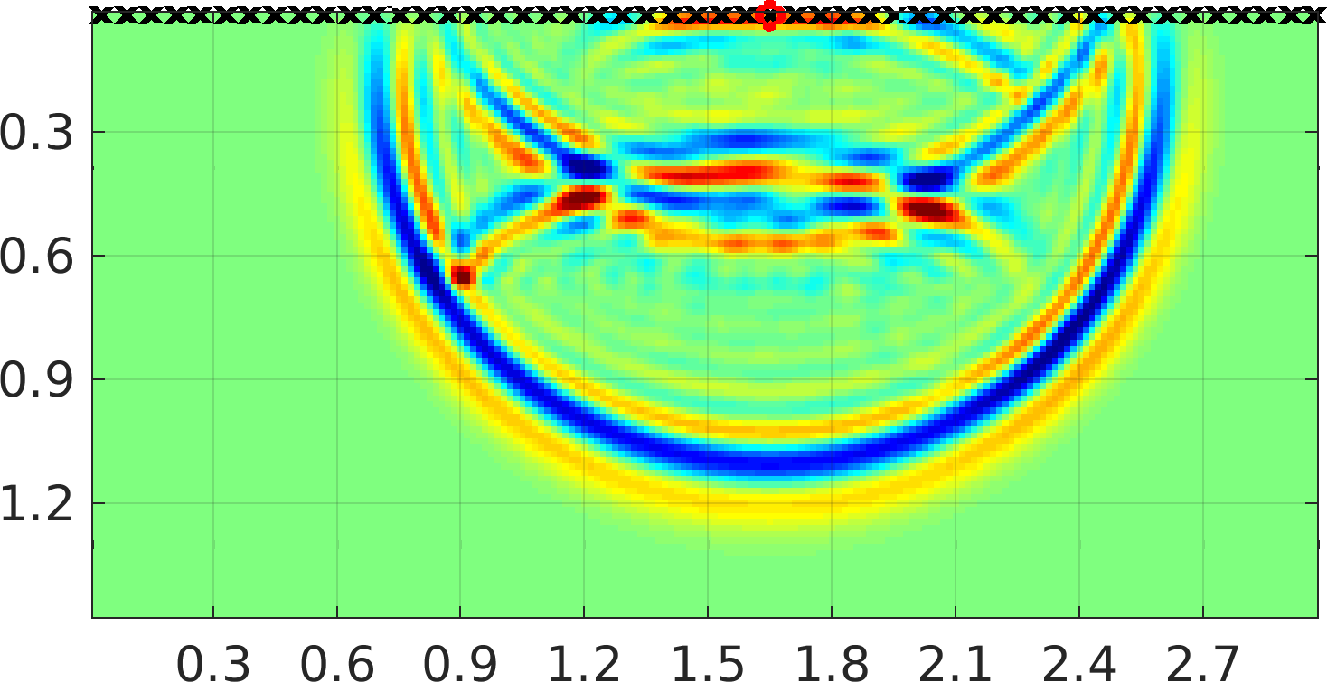
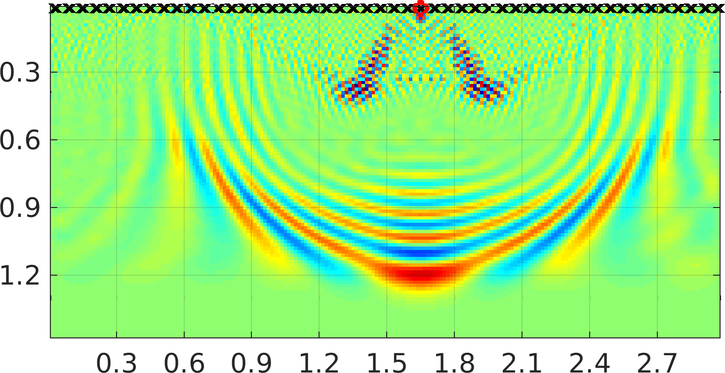
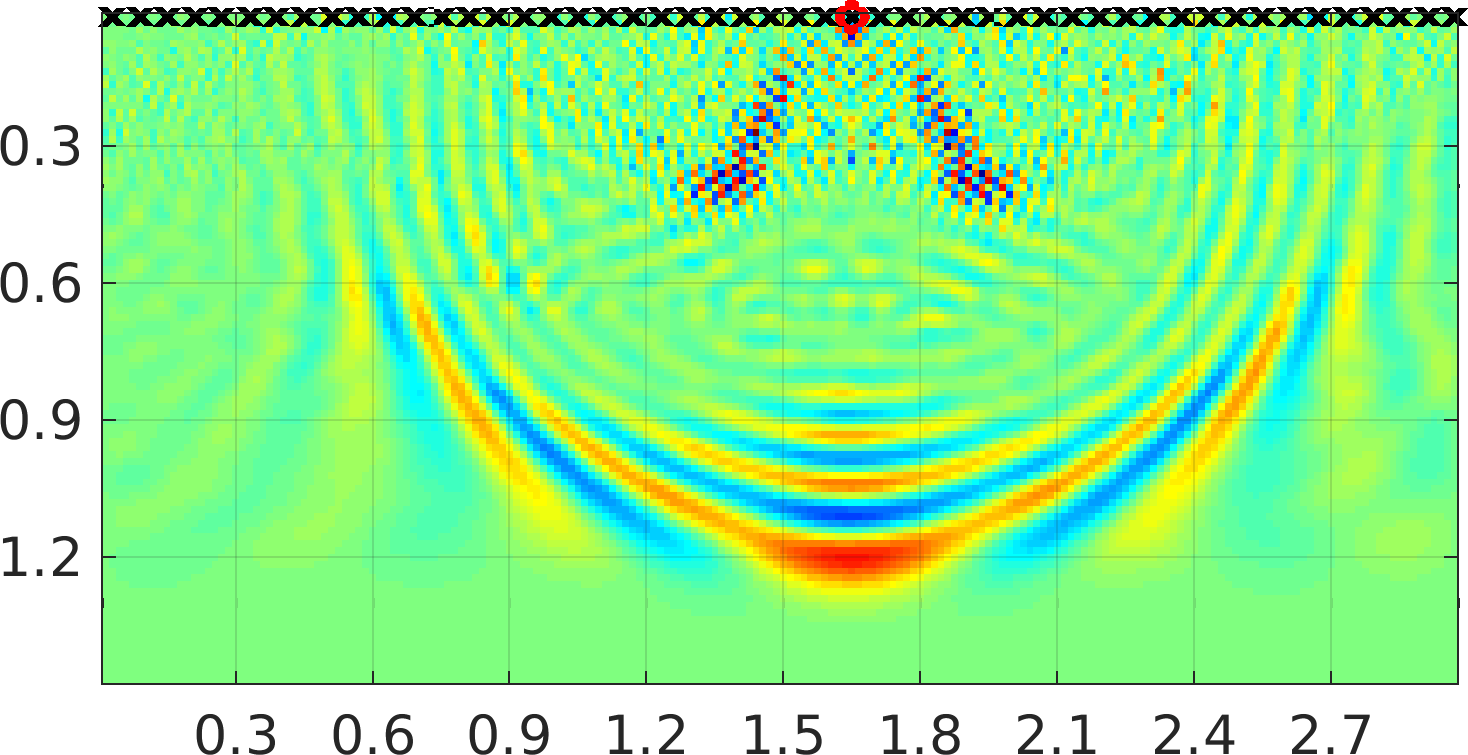
Figure 5. Primary snapshots and their orthonormal counterparts for the reference medium with $\sigma^{0}({{\itbf x}})\equiv 1$ and the true medium. For every snapshot we plot a single column of the $N\times mn$ matrices, corresponding to the source $j=28$ (red $\circ$) out of $m=50$ sensors in the array (black $\times$). The rows (top to bottom) correspond to times $t_{k}=k\tau$, for $k=25,30$. The axes are in km units.

In Figure 5 we plot the primary snapshots at two time instances $t_{k}=k\tau$, with $k=25$ and $k=30$, for the reference medium with $\sigma^{0}\equiv 1$ and the scattering medium displayed in Figure 4. We also display the orthonormal snapshots. The primary snapshots in the reference medium (first column) show the wavefront. In the scattering medium (second column) there are multiple reflections behind the wavefront. The orthonormal snapshots for both media (third and forth columns) have a “smile-like” shape with a “thick lower lip”. They can be viewed as approximations of delta functions. The reflections are suppressed in the orthonormal snapshots, and we note that they are almost the same in both media i.e., they are almost independent of $\sigma$. A similar result holds for the dual snapshots, not shown here.

Scattered data	Born approximation	DtB

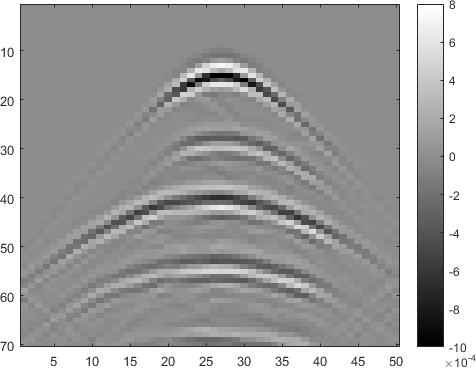
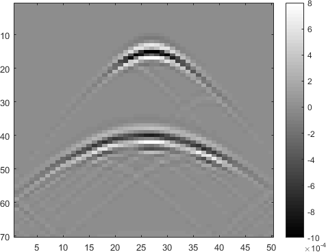
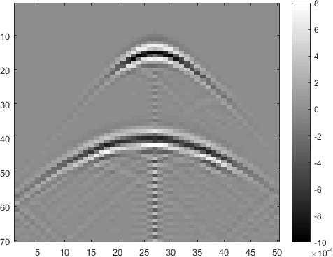
Figure 6. From left to right: raw scattered data, Born approximation and the data transformed by the DtB algorithm. The abscissa is the sensor index, and the ordinate is the index $k$ of the discrete time instants $t_{k}=\tau k$, $\tau=0.034s$.

In the left plot of Figure 6 we display the raw scattered data at the sensors, due to the excitation from the sensor at the center of the linear array, lying just below the top boundary. The Born approximation and the data transformed by the DtB algorithm are in the middle and right plots. The results are almost the same. To illustrate better the agreement between the Born approximation and the output of the DtB algorithm, we display in Figure 7 a comparison of several traces (signals at certain receivers) from Figure 6.

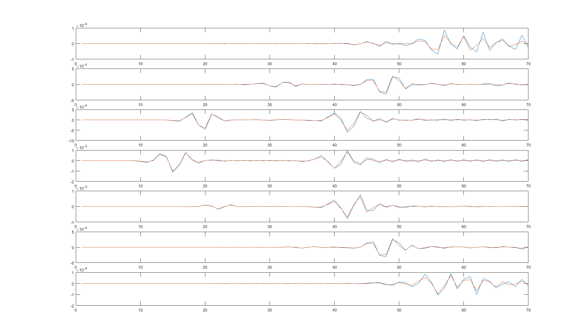
Figure 7. Comparison of a few traces of the Born approximation (red) and the DtB algorithm output (blue) from Figure 6. The abscissa is the time index.

Image with raw data	Image with DtB transformed data

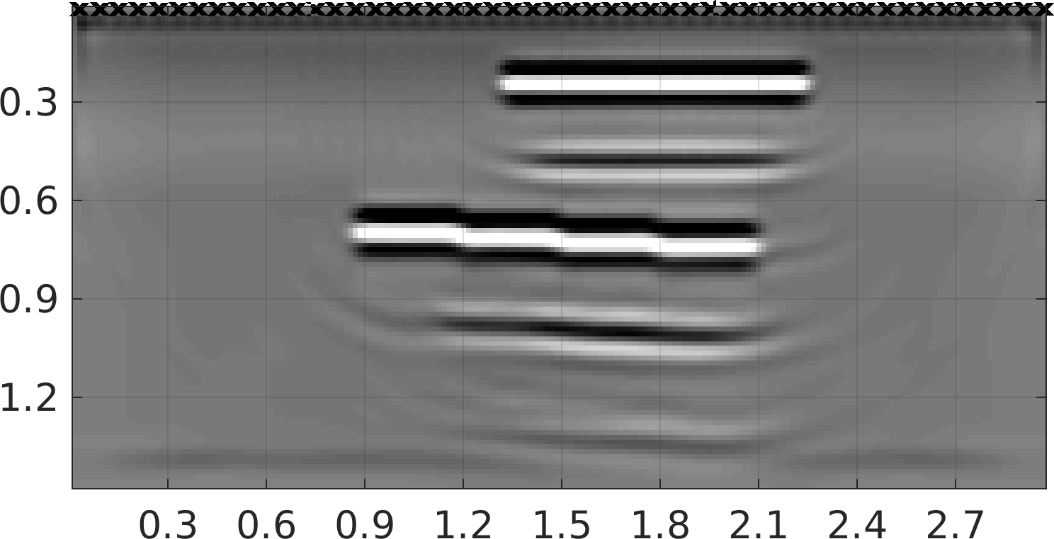
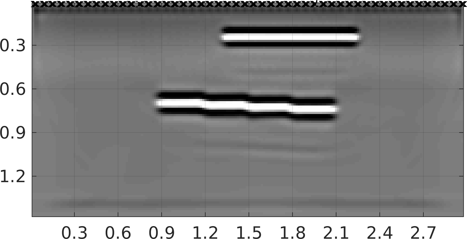
Figure 8. Reverse time migration image obtained with the raw data (left) and the data transformed with the DtB algorithm (right). The axes are in km units, as in Figure 4.

To illustrate the benefit of the DtB transformation on imaging, we display in Figure 8 the reverse time migration images obtained with the raw data and the transformed data shown in the left and right plots of Figure 6. The artifacts due to multiple scattering are evident in the image shown on the left, which displays multiple ghost reflectors. The image obtained with the transformed data, shown on the right, does not have multiple artifacts and localizes well the two reflectors.

As we mentioned in the introduction, in practice only the smooth part of $c({{\itbf x}})$ may be known. To illustrate that the DtB algorithm can deal with perturbations of the sound speed, we present in Figure 9 numerical results for three inclusions embedded in a medium with constant wave speed $c_{0}=1$km/s and constant density $\rho$. The inclusions are modeled by the variation of $c({{\itbf x}})$ displayed in the left plot, but the density is kept constant i.e., $\sigma({{\itbf x}})=\rho c({{\itbf x}})$. Only $c_{0}$ is assumed known in the DtB algorithm, meaning that we used the incorrect speed $c_{0}$ instead of the true $c({{\itbf x}})$. The data gathered by the array, for the excitation from the source shown with a red circle in the left plot, are displayed in the middle plot. They contain the primary reflections from each inclusion and multiply scattered reflections between the inclusions. The output of the DtB algorithm is displayed in the right plot of Figure 9. The multiply scattered echoes are removed and there are three, clearly separated echoes, corresponding to each inclusion. Note the unmasking of the second echo, due to the smaller inclusion, that was mixed with a multiply scattered echo in the middle plot.

Model $c({{\itbf x}})$	Scattered data	DtB

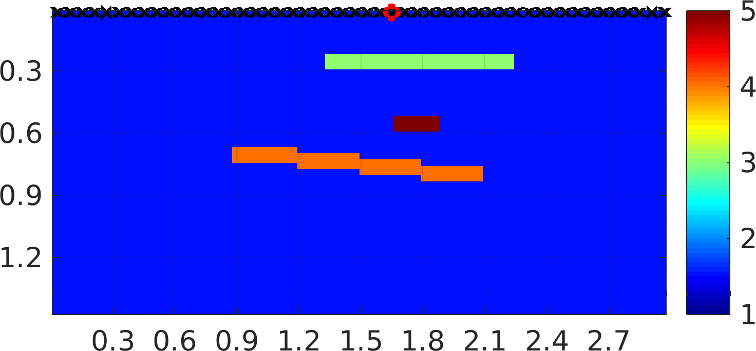
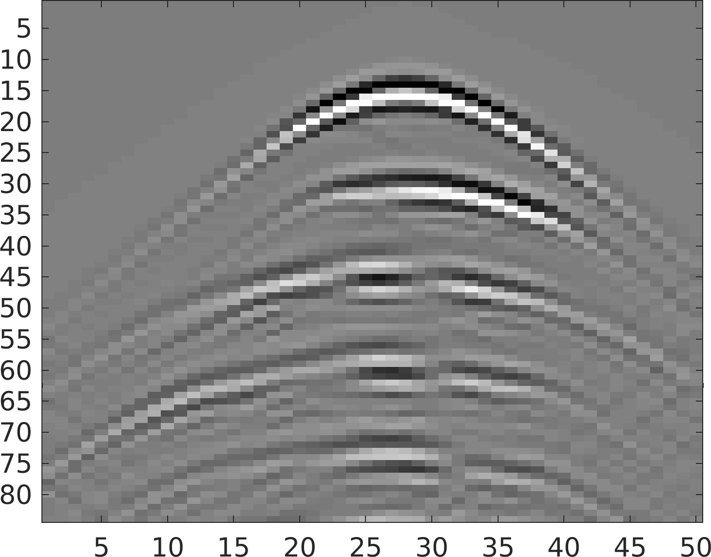
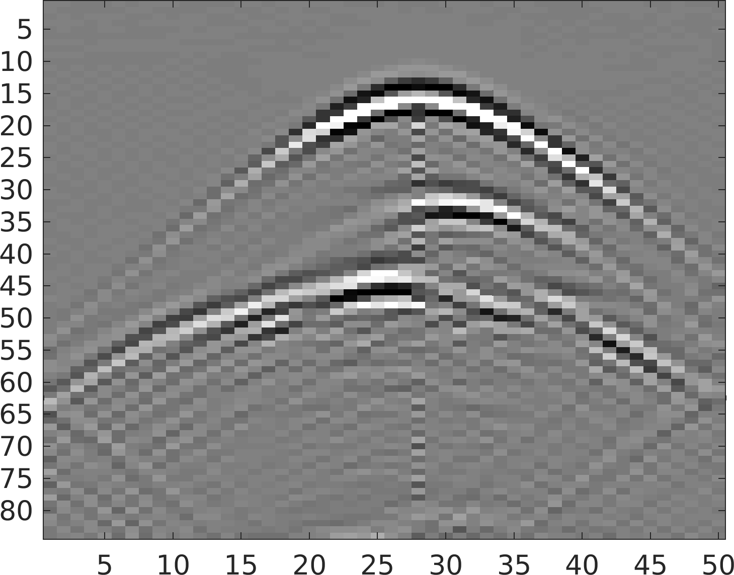
Figure 9. Left: model of a medium with three inclusions. The value of the wave speed $c({{\itbf x}})$ is shown in the color bar, in units of km/s. The axes are in km units and the array sits on the top, as in the previous simulations. Middle: Data gathered for a single source shown as red $\circ$ in the left figure. The abscissa is the sensor receiver index and the ordinate is the discrete time sample with step $\tau=0.0225s$. Right: the result of the DtB algorithm.

5. Summary

This paper is motivated by the inverse scattering problem for the wave equation, where an array of sensors probes an unknown scattering medium with pulses and measures the reflected waves. The goal of the inversion is to estimate the perturbations of the acoustic impedance in the medium, which cause wave scattering. We introduced a direct, linear-algebra based algorithm, called the Data to Born (DtB) algorithm, for transforming the data collected by the array to data corresponding to the single scattering (Born) approximation. These data can then be used by any off-the-shelf algorithms that incorporate state of the art linear inversion methodologies. The key ingredient in the DtB algorithm is a data driven, reduced order model (ROM), that approximates the wave propagator operator. Because the DtB algorithm involves only linear algebra operations, like matrix-matrix multiplications and block Cholesky factorizations, the cost of the algorithm is $O((mn)^{3})$, where $m$ is the number of sensors and $2n$ is the number of time samples in the measurements. However, due to the Toeplitz-plus-Hankel structure of the mass and stiffness matrices, this cost can be reduced, possibly to $O(m^{3}n^{2}\log n)$. This will be a subject of future research.

Appendix A The tridiagonal structure of the ROM propagator

In this appendix we show that the the ROM propagator given by the projection (71) is a tridiagonal matrix. Obviously, $\widetilde{\boldsymbol{{\mathscr{P}}}}$ is symmetric, so it suffices to show that its entries

$$(\widetilde{\boldsymbol{{\mathscr{P}}}})_{j+l,j}={\itbf V}_{j+l}^{T}\boldsymbol{{\mathscr{P}}}{\itbf V}_{j}$$ (157)

are zero when $l\geq 2$.

We obtain from equation (78) that $\displaystyle{\itbf V}_{j}=\sum_{i=0}^{j-1}({\itbf R}^{-1})_{i+1,j}\boldsymbol{{P}}_{i},$ where we used that the inverse ${\itbf R}^{-1}$ of the upper triangular matrix ${\itbf R}$ is upper triangular. The relation (75) satisfied by the Chebyshev polynomials and definition (64) give

$$\boldsymbol{{\mathscr{P}}}\boldsymbol{{P}}_{i}=\mathcal{T}_{1}(\boldsymbol{{\mathscr{P}}})\mathcal{T}_{i}(\boldsymbol{{\mathscr{P}}}){\itbf b}=\frac{1}{2}\Big{[}\mathcal{T}_{i+1}(\boldsymbol{{\mathscr{P}}})+\mathcal{T}_{|i-1|}(\boldsymbol{{\mathscr{P}}})\Big{]}{\itbf b}=\frac{1}{2}\big{(}\boldsymbol{{P}}_{i+1}+\boldsymbol{{P}}_{|i-1|}\big{)},$$ (158)

so equation (157) becomes

$$(\widetilde{\boldsymbol{{\mathscr{P}}}})_{j+l,j}=\frac{1}{2}\sum_{i=0}^{j-1}({\itbf R}^{-1})_{i+1,j}\Big{(}{\itbf V}_{j+l}^{T}\boldsymbol{{P}}_{i+1}+{\itbf V}_{j+l}^{T}\boldsymbol{{P}}_{|i-1|}\Big{)}.$$ (159)

Each term in this sum can be calculated from (72) as ${\itbf V}_{j+l}^{T}\boldsymbol{{P}}_{i}=({\itbf R})_{j+l,i+1},$ so we obtain

$$(\widetilde{\boldsymbol{{\mathscr{P}}}})_{j+l,j}=\frac{1}{2}\sum_{i=0}^{j-1}({\itbf R}^{-1})_{i+1,j}\Big{[}({\itbf R})_{j+l,i+2}+({\itbf R})_{j+l,|i-1|+1}\Big{)}.$$ (160)

Note that $j+l>\max\{i+2,|i-1|+1\}$ when $l\geq 2$ and $i=0,\ldots,j-1$, so the right hand side in (160) is zero by the upper triangular structure of ${\itbf R}$. This means that $\widetilde{\boldsymbol{{\mathscr{P}}}}$ is tridiagonal.

Appendix B Computation of the block-bidiagonal $\widetilde{{\itbf L}}_{q}$

We describe the computation of the block-Cholesky factor $\widetilde{{\itbf L}}_{q}$ using an approach outlined in [21]. As mentioned in section 4.5, the block Cholesky factorization is not uniquely defined. Clearly, if ${\itbf Q}_{k}={\itbf I}_{m},$ the diagonal blocks ${\itbf R}_{k,k},$ are symmetric, for $k=1,\ldots,n.$ We denote the corresponding MIMO ROM matrix given by (79) as $\widetilde{\boldsymbol{{\mathscr{P}}}}^{{\itbf I}}$.

For non-trivial orthogonal matrices ${\itbf Q}_{k}$, the MIMO ROM matrix $\widetilde{\boldsymbol{{\mathscr{P}}}}^{{\itbf Q}}$ is given by ${\itbf Q}\widetilde{\boldsymbol{{\mathscr{P}}}}^{{\itbf I}}{\itbf Q}^{T}$ where ${\itbf Q}$ is the block-diagonal matrix with orthogonal blocks ${\itbf Q}_{k}$, $k=1,\ldots,n$. However, the block bidiagonal factor $\widetilde{{\itbf L}}_{q}$ in (82) has to be consistent with the matrix analogue of the recursion (95)–(97) for computing the primary and dual orthogonalized block snapshots $\overline{\bf p}_{j}\in\mathbb{R}^{N\times m}$ and $\overline{\bf u}_{j}\in\mathbb{R}^{N\times m}$,

$${\boldsymbol{\gamma}}^{-1}_{j}\left(\overline{\bf p}_{j+1}-\overline{\bf p}_{j}\right)=-\boldsymbol{\mathcal{L}}_{q}\overline{\bf u}_{j},\quad{\widehat{\boldsymbol{\gamma}}}^{-1}_{j}\left(\overline{\bf u}_{j}-\overline{\bf u}_{j-1}\right)=\boldsymbol{\mathcal{L}}_{q}^{T}\overline{\bf p}_{j},\quad j\geq 1,$$ (161)

with initial conditions $\overline{\bf p}_{1}={\itbf b}$ and $\overline{\bf u}_{0}=0,$ and symmetric positive definite matrix coefficients

$$0<{\boldsymbol{\gamma}}_{j}={\boldsymbol{\gamma}}^{T}_{j}=\Big{(}\overline{\bf u}_{j}^{T}\overline{\bf u}_{j}\Big{)}^{-1}\in\mathbb{R}^{m\times m},\quad 0<{\widehat{\boldsymbol{\gamma}}}_{j}={\widehat{\boldsymbol{\gamma}}}^{T}_{j}=\Big{(}\overline{\bf p}_{j}^{T}\overline{\bf p}_{j}\Big{)}^{-1}\in\mathbb{R}^{m\times m},$$ (162)

for $j=1,\ldots,n$. Then,

$$(\widetilde{{\itbf L}}_{q})_{j,j} =-\sqrt{{\widehat{\boldsymbol{\gamma}}}^{-1}_{j}}\sqrt{{\boldsymbol{\gamma}}^{-1}_{j}},~{}~{}1\leq j\leq n,\quad(\widetilde{{\itbf L}}_{q})_{j+1,j}=\sqrt{{\widehat{\boldsymbol{\gamma}}}^{-1}_{j+1}}\sqrt{{\boldsymbol{\gamma}}^{-1}_{j}}~{}~{}1\leq j\leq n-1.$$ (163)

We now determine the matrix ${\itbf Q}$ such that the factorization

$$\xi\Big{(}{\itbf Q}\widetilde{\boldsymbol{{\mathscr{P}}}}^{{\itbf I}}{\itbf Q}^{T}\Big{)}={\itbf Q}\xi\Big{(}\widetilde{\boldsymbol{{\mathscr{P}}}}^{{\itbf I}}\Big{)}{\itbf Q}^{T}=\widetilde{{\itbf L}}_{q}\widetilde{{\itbf L}}^{T}_{q},$$ (164)

corresponds to $\widetilde{{\itbf L}}_{q}$ of the form (163) with symmetric positive definite ${\boldsymbol{\gamma}}_{j}$ and ${\widehat{\boldsymbol{\gamma}}}_{j}$, $j=1,\ldots,n$.

Denote the diagonal and the off-diagonal blocks of $\xi\Big{(}\widetilde{\boldsymbol{{\mathscr{P}}}}^{{\itbf I}}\Big{)}$ by ${\boldsymbol{\alpha}}_{j}\in\mathbb{R}^{m\times m}$, for $j=1,\ldots,n$ and ${\boldsymbol{\beta}}_{j}\in\mathbb{R}^{m\times m}$, for $j=2,\ldots,n$. By definition,

$${\widehat{\boldsymbol{\gamma}}}_{1}=({\itbf b}^{T}{\itbf b})^{-1}.$$ (165)

The remaining matrix coefficients ${\boldsymbol{\gamma}}_{j}$ and ${\widehat{\boldsymbol{\gamma}}}_{j}$ are obtained from (164) block-wise. From the first diagonal block we obtain that $\sqrt{{\widehat{\boldsymbol{\gamma}}}^{-1}_{1}}{\boldsymbol{\gamma}}^{-1}_{1}\sqrt{{\widehat{\boldsymbol{\gamma}}}^{-1}_{1}}={\itbf Q}_{1}{\boldsymbol{\alpha}}_{1}{\itbf Q}^{T}_{1}$ or, equivalently,

$${\boldsymbol{\gamma}}_{1}=\left(\sqrt{{\widehat{\boldsymbol{\gamma}}}_{1}}{\itbf Q}_{1}{\boldsymbol{\alpha}}_{1}{\itbf Q}^{T}_{1}\sqrt{{\widehat{\boldsymbol{\gamma}}}_{1}}\right)^{-1}.$$ (166)

Clearly, ${\boldsymbol{\gamma}}_{1}={\boldsymbol{\gamma}}^{T}_{1}$ for any matrix ${\itbf Q}_{1}$, so for simplicity we set ${\itbf Q}_{1}={\itbf I}_{m}$. Then, from the off-diagonal blocks for $1\leq j\leq n-1$ we have $\sqrt{{\widehat{\boldsymbol{\gamma}}}^{-1}_{j}}{\boldsymbol{\gamma}}^{-1}_{j}\sqrt{{\widehat{\boldsymbol{\gamma}}}^{-1}_{j+1}}={\itbf Q}_{j}{\boldsymbol{\beta}}_{j+1}{\itbf Q}^{T}_{j+1}$. Hence, $\sqrt{{\widehat{\boldsymbol{\gamma}}}^{-1}_{j+1}}{\itbf Q}_{j+1}={\boldsymbol{\gamma}}_{j}\sqrt{{\widehat{\boldsymbol{\gamma}}}_{j}}{\itbf Q}_{j}{\boldsymbol{\beta}}_{j+1}$. That is to say, the pair of matrices $\sqrt{{\widehat{\boldsymbol{\gamma}}}^{-1}_{j+1}}$ and ${\itbf Q}_{j+1}$ is a (left) polar decomposition of ${\itbf M}_{j}={\boldsymbol{\gamma}}_{j}\sqrt{{\widehat{\boldsymbol{\gamma}}}_{j}}{\itbf Q}_{j}{\boldsymbol{\beta}}_{j+1}.$ Its solution is

$${\widehat{\boldsymbol{\gamma}}}_{j+1} =\left({\itbf M}_{j}{\itbf M}^{T}_{j}\right)^{-1},\quad{\itbf Q}_{j+1}=\sqrt{{\widehat{\boldsymbol{\gamma}}}_{j+1}}{\itbf M}_{j}.$$ (167)

Finally, considering the diagonal blocks for $1\leq j\leq n-1$, we obtain

$$\sqrt{{\widehat{\boldsymbol{\gamma}}}^{-1}_{j+1}}\left({\boldsymbol{\gamma}}^{-1}_{j}+\gamma^{-1}_{j+1}\right)\sqrt{{\widehat{\boldsymbol{\gamma}}}^{-1}_{j+1}}={\itbf Q}_{j+1}{\boldsymbol{\alpha}}_{j+1}{\itbf Q}^{T}_{j+1}$$

and therefore

$${\boldsymbol{\gamma}}_{j+1}=\left(\sqrt{{\widehat{\boldsymbol{\gamma}}}_{j+1}}{\itbf Q}_{j+1}{\boldsymbol{\alpha}}_{j+1}{\itbf Q}^{T}_{j+1}\sqrt{{\widehat{\boldsymbol{\gamma}}}_{j+1}}-{\boldsymbol{\gamma}}^{-1}_{j}\right)^{-1}.$$ (168)

Algorithm B.1 (Computation of $\widetilde{{\itbf L}}_{q}$).

Input: the block tridiagonal matrix $\widetilde{\boldsymbol{{\mathscr{P}}}}^{{\itbf I}}\in\mathbb{R}^{nm\times nm}$ with $m\times m$ blocks and ${\itbf b}^{T}{\itbf b}$.

To find a block diagonal ${\itbf Q}$ such that the block Cholesky factorization $\widetilde{{\itbf L}}_{q}\widetilde{{\itbf L}}^{T}_{q}$ of $\xi\Big{(}\widetilde{\boldsymbol{{\mathscr{P}}}}^{{\itbf Q}}\Big{)}$ has factors $\widetilde{{\itbf L}}_{q}$ in the form (163), perform the following steps:

1. Compute ${\widehat{\boldsymbol{\gamma}}}_{1}$ via (165) and ${\boldsymbol{\gamma}}_{1}$ via (166) for arbitrary ${\itbf Q}_{1}$ (for simplicity, we set ${\itbf Q}_{1}={\itbf I}_{m}$)

2. For $j=1,\ldots,n-1:$ Compute ${\widehat{\boldsymbol{\gamma}}}_{j+1}$ and ${\itbf Q}_{j+1}$ via (167) and ${\boldsymbol{\gamma}}_{j+1}$ via (168).

3. Compute $\widetilde{{\itbf L}}_{q}$ via (163)

Output: the block diagonal orthogonal matrix ${\itbf Q}$, the block tridiagonal propagator matrix $\widetilde{\boldsymbol{{\mathscr{P}}}}^{{\itbf Q}}={\itbf Q}\widetilde{\boldsymbol{{\mathscr{P}}}}^{{\itbf I}}{\itbf Q}^{T}$ and the block lower bidiagonal factor $\widetilde{{\itbf L}}_{q}$ of $\xi\Big{(}\widetilde{\boldsymbol{{\mathscr{P}}}}^{{\itbf Q}}\Big{)}$ consistent with (163).

References

- [1] R. Alonso, L. Borcea, G. Papanicolaou, and C. Tsogka, Detection and imaging in strongly backscattering randomly layered media, Inverse Problems, 27 (2011), p. 025004.
- [2] A. Aubry and A. Derode, Detection and imaging in a random medium: A matrix method to overcome multiple scattering and aberration, Journal of Applied Physics, 106 (2009), p. 044903.
- [3] G. Beylkin, Imaging of discontinuities in the inverse scattering problem by inversion of a causal generalized Radon transform, Journal of Mathematical Physics, 26 (1985), pp. 99–108.
- [4] G. Beylkin and R. Burridge, Linearized inverse scattering problems in acoustics and elasticity, Wave motion, 12 (1990), pp. 15–52.
- [5] B. Biondi, 3D seismic imaging, Society of Exploration Geophysicists, 2006.
- [6] L. Borcea, F. G. Del Cueto, G. Papanicolaou, and C. Tsogka, Filtering random layering effects in imaging, Multiscale Modeling & Simulation, 8 (2010), pp. 751–781.
- [7] L. Borcea, F. G. del Cueto, G. Papanicolaou, and C. Tsogka, Filtering deterministic layer effects in imaging, SIAM Review, 54 (2012), pp. 757–798.
- [8] L. Borcea, V. Druskin, and L. Knizhnerman, On the continuum limit of a discrete inverse spectral problem on optimal finite difference grids, Communications on Pure and Applied Mathematics, 58 (2005), pp. 1231–1279.
- [9] L. Borcea, V. Druskin, A. V. Mamonov, and M. Zaslavsky, A model reduction approach to numerical inversion for a parabolic partial differential equation, Inverse Problems, 30 (2014), p. 125011.
- [10] L. Borcea, V. Druskin, F. G. Vasquez, and A. Mamonov, Resistor network approaches to electrical impedance tomography, Inverse Problems and Applications: Inside Out II, Math. Sci. Res. Inst. Publ, 60 (2011), pp. 55–118.
- [11] L. Borcea, G. Papanicolaou, and C. Tsogka, Adaptive time-frequency detection and filtering for imaging in heavy clutter, SIAM Journal on Imaging Sciences, 4 (2011), pp. 827–849.
- [12] K. P. Bube and R. Burridge, The one-dimensional inverse problem of reflection seismology, SIAM review, 25 (1983), pp. 497–559.
- [13] R. Burridge, The Gelfand-Levitan, the Marchenko, and the Gopinath-Sondhi integral equations of inverse scattering theory, regarded in the context of inverse impulse-response problems, Wave motion, 2 (1980), pp. 305–323.
- [14] M. Cheney and B. Borden, Fundamentals of radar imaging, vol. 79, SIAM, 2009.
- [15] M. T. Chu and G. H. Golub, Structured inverse eigenvalue problems, Acta Numerica, 11 (2002), p. 1.
- [16] F. Delprat-Jannaud and P. Lailly, A fundamental limitation for the reconstruction of impedance profiles from seismic data, Geophysics, 70 (2005), pp. R1–R14.
- [17] B. W. Drinkwater and P. D. Wilcox, Ultrasonic arrays for non-destructive evaluation: A review, Ndt & E International, 39 (2006), pp. 525–541.
- [18] V. Druskin, S. Güttel, and L. Knizhnerman, Near-optimal perfectly matched layers for indefinite helmholtz problems, SIAM Review, 58 (2016), pp. 90–116.
- [19] V. Druskin and L. Knizhnerman, Gaussian spectral rules for the three-point second differences: I. a two-point positive definite problem in a semi-infinite domain, SIAM Journal on Numerical Analysis, 37 (1999), pp. 403–422.
- [20] V. Druskin, A. V. Mamonov, A. E. Thaler, and M. Zaslavsky, Direct, nonlinear inversion algorithm for hyperbolic problems via projection-based model reduction, SIAM Journal on Imaging Sciences, 9 (2016), pp. 684–747.
- [21] V. Druskin, A. V. Mamonov, and M. Zaslavsky, Multiscale S-Fraction Reduced-Order Models for Massive Wavefield Simulations, Multiscale Modeling & Simulation, 15 (2017), pp. 445–475.
- [22] V. Druskin, A. V. Mamonov, and M. Zaslavsky, A nonlinear method for imaging with acoustic waves via reduced order model backprojection, SIIMS in press, arXiv:1704.06974 [math.NA], (2017).
- [23] Y. M. Dyukarev, Indeterminacy criteria for the stieltjes matrix moment problem, Mathematical Notes, 75 (2004), pp. 66–82.
- [24] S. Fomel, E. Landa, and M. T. Taner, Poststack velocity analysis by separation and imaging of seismic diffractions, Geophysics, 72 (2007), pp. U89–U94.
- [25] K. Gallivan, E. Grimme, D. Sorensen, and P. Van Dooren, On some modifications of the Lanczos algorithm and the relation with Padé approximations, Mathematical Research, 87 (1996), pp. 87–116.
- [26] K. Gallivan, G. Grimme, and P. Van Dooren, A rational Lanczos algorithm for model reduction, Numerical Algorithms, 12 (1996), pp. 33–63.
- [27] I. M. Gel’fand and B. M. Levitan, On the determination of a differential equation from its spectral function, in Amer. Math. Soc. Transl., AMS, Providence, RI, 1955, pp. 253–304.
- [28] H. G. Golub and C. F. Van Loan, Matrix computations, The Johns Hopkins University Press, Baltimore and London, 3 ed., 1996.
- [29] B. Gopinath and M. Sondhi, Inversion of the telegraph equation and the synthesis of nonuniform lines, Proceedings of the IEEE, 59 (1971), pp. 383–392.
- [30] T. M. Habashy, A generalized Gel’fand-Levitan-Marchenko integral equation, Inverse Problems, 7 (1991), p. 703.
- [31] S. I. Kabanikhin and M. A. Shishlenin, Numerical algorithm for two-dimensional inverse acoustic problem based on Gel’fand–Levitan–Krein equation, Journal of Inverse and Ill-Posed Problems, 18 (2011), pp. 979–995.
- [32] I. Kac and M. Krein, On the spectral functions of the string, Amer. Math. Soc. Transl, 103 (1974), pp. 19–102.
- [33] M. G. Krein, Solution of the inverse Sturm-Liouville problem, in Dokl. Akad. Nauk SSSR, vol. 76 (1), 1951, pp. 21–24.
- [34] , On the transfer function of a one-dimensional boundary problem of second order, in Dokl. Akad. Nauk SSSR, vol. 88, 1953, pp. 405–408.
- [35] Z. Liu and N. Bleistein, Migration velocity analysis: Theory and an iterative algorithm, Geophysics, 60 (1995), pp. 142–153.
- [36] A. E. Malcolm, M. V. de Hoop, and H. Calandra, Identification of image artifacts from internal multiples, Geophysics, 72 (2007), pp. S123–S132.
- [37] V. A. Marchenko, Some problems in the theory of one-dimensional second-order differential operators, Dokl. Akad. Nauk. SSSR, 2 (1950), pp. 457–560.
- [38] S. Moskow, K. Kilgore, and J. C. Schotland, Inverse Born series for scalar waves, Journal of Computational Mathematics, 30 (2012), pp. 601–614.
- [39] B. N. Parlett, The symmetric eigenvalue problem, SIAM, 1998.
- [40] Rakesh, A linearised inverse problem for the wave equation, Communications in Partial Differential Equations, 13 (1988), pp. 573–601.
- [41] T. J. Rivlin, Chebyshev polynomials., John Wiley & Sons, Inc., 1990.
- [42] F. Santosa, Numerical scheme for the inversion of acoustical impedance profile based on the Gelfand-Levitan method, Geophysical Journal International, 70 (1982), pp. 229–243.
- [43] C. C. Stolk and W. W. Symes, Smooth objective functionals for seismic velocity inversion, Inverse Problems, 19 (2002), p. 73.
- [44] W. Symes, Inverse boundary value problems and a theorem of Gel’fand and Levitan, Journal of Mathematical Analysis and Applications, 71 (1979), pp. 379–402.
- [45] W. W. Symes, Mathematics of reflection seismology. The Rice Inversion Project, Department of Computational and Applied Mathematics, Rice University, http://trip.rice.edu/downloads/preamble.pdf, 1995.
- [46] W. W. Symes, The seismic reflection inverse problem, Inverse problems, 25 (2009), p. 123008.
- [47] C. W. Therrien, Discrete random signals and statistical signal processing, Prentice Hall PTR, 1992.
- [48] G. Uhlmann, Travel time tomography, Journal of the Korean Mathematical Society, 38 (2001), pp. 711–722.
- [49] K. Wapenaar, F. Broggini, E. Slob, and R. Snieder, Three-dimensional single-sided Marchenko inverse scattering, data-driven focusing, Green’s function retrieval, and their mutual relations, Physical Review Letters, 110 (2013), p. 084301.
- [50] K. Wapenaar, J. Thorbecke, J. Van Der Neut, F. Broggini, E. Slob, and R. Snieder, Marchenko imaging, Geophysics, 79 (2014), pp. WA39–WA57.
- [51] A. B. Weglein, Multiple attenuation: an overview of recent advances and the road ahead, The Leading Edge, 18 (1999), pp. 40–44.