From Fixed-X to Random-X Regression: Bias-Variance Decompositions, Covariance Penalties, and Prediction Error Estimation

Abstract

In statistical prediction, classical approaches for model selection and model evaluation based on covariance penalties are still widely used. Most of the literature on this topic is based on what we call the “Fixed-X” assumption, where covariate values are assumed to be nonrandom. By contrast, it is often more reasonable to take a “Random-X” view, where the covariate values are independently drawn for both training and prediction. To study the applicability of covariance penalties in this setting, we propose a decomposition of Random-X prediction error in which the randomness in the covariates contributes to both the bias and variance components. This decomposition is general, but we concentrate on the fundamental case of least squares regression. We prove that in this setting the move from Fixed-X to Random-X prediction results in an increase in both bias and variance. When the covariates are normally distributed and the linear model is unbiased, all terms in this decomposition are explicitly computable, which yields an extension of Mallows’ Cp that we call RCp. RCp also holds asymptotically for certain classes of nonnormal covariates. When the noise variance is unknown, plugging in the usual unbiased estimate leads to an approach that we call $\widehat{{\rm RCp}}$, which is closely related to Sp (Tukey 1967), and GCV (Craven and Wahba 1978). For excess bias, we propose an estimate based on the “shortcut-formula” for ordinary cross-validation (OCV), resulting in an approach we call RCp⁺. Theoretical arguments and numerical simulations suggest that RCp⁺ is typically superior to OCV, though the difference is small. We further examine the Random-X error of other popular estimators. The surprising result we get for ridge regression is that, in the heavily-regularized regime, Random-X variance is smaller than Fixed-X variance, which can lead to smaller overall Random-X error.

1 Introduction

A statistical regression model seeks to describe the relationship between a response $y\in\mathbb{R}$ and a covariate vector $x\in\mathbb{R}^{p}$, based on training data comprised of paired observations $(x_{1},y_{1}),\ldots,(x_{n},y_{n})$. Many modern regression models are ultimately aimed at prediction: given a new covariate value $x_{0}$, we apply the model to predict the corresponding response value $y_{0}$. Inference on the prediction error of regression models is a central part of model evaluation and model selection in statistical learning (e.g., Hastie et al. 2009). A common assumption that is used in the estimation of prediction error is what we call a “Fixed-X” assumption, where the training covariate values $x_{1},\ldots,x_{n}$ are treated as fixed, i.e., nonrandom, as are the covariate values at which predictions are to be made, $x_{01},\ldots,x_{0n}$, which are also assumed to equal the training values. In the Fixed-X setting, the celebrated notions of optimism and degrees of freedom lead to covariance penalty approaches to estimate the prediction performance of a model (Efron, 1986, 2004; Hastie et al., 2009), extending and generalizing classical approaches like Mallows’ Cp (Mallows, 1973) and AIC (Akaike, 1973).

The Fixed-X setting is one of the most common views on regression (arguably the predominant view), and it can be found at all points on the spectrum from cutting-edge research to introductory teaching in statistics. This setting combines the following two assumptions about the problem.

1. The covariate values $x_{1},\ldots,x_{n}$ used in training are not random (e.g., designed), and the only randomness in training is due to the responses $y_{1},\ldots,y_{n}$.

2. The covariates $x_{01},\ldots,x_{0n}$ used for prediction exactly match $x_{1},\ldots,x_{n}$, respectively, and the corresponding responses $y_{01},\ldots,y_{0n}$ are independent copies of $y_{1},\ldots,y_{n}$, respectively.

Relaxing assumption (i), i.e., acknowledging randomness in the training covariates $x_{1},\ldots,x_{n}$, and taking this randomness into account when performing inference on estimated parameters and fitted models, has received a good deal of attention in the literature. But, as we see it, assumption (ii) is the critical one that needs to be relaxed in most realistic prediction setups. To emphasize this, we define two settings beyond the Fixed-X one, that we call the “Same-X” and “Random-X” settings. The Same-X setting drops assumption (i), but does not account for new covariate values at prediction time. The Random-X setting drops both assumptions, and deals with predictions at new covariates values. These will be defined more precisely in the next subsection.

1.1 Notation and assumptions

We assume that the training data $(x_{1},y_{1}),\ldots,(x_{n},y_{n})$ are i.i.d. according to some joint distribution $P$. This is an innocuous assumption, and it means that we can posit a relationship for the training data,

$$y_{i}=f(x_{i})+\epsilon_{i},\quad i=1,\ldots,n$$ (1)

where $f(x)=\mathbb{E}(y|x)$, and the expectation here is taken with respect to a draw $(x,y)\sim P$. We also assume that for $(x,y)\sim P$,

$$\text{$\epsilon=y-f(x)$ is independent of $x$},$$ (2)

which is less innocuous, and precludes, e.g., heteroskedasticity in the data. We let $\sigma^{2}=\mathrm{Var}(y|x)$ denote the constant conditional variance. It is worth pointing out that some results in this paper can be adjusted or modified to hold when (2) is not assumed; but since other results hinge critically on (2), we find it is more convenient to assume (2) up front.

For brevity, we write $Y=(y_{1},\ldots,y_{n})\in\mathbb{R}^{n}$ for the vector of training responses, and $X\in\mathbb{R}^{n\times p}$ for the matrix of training covariates with $i$th row $x_{i}$, $i=1,\ldots,n$. We also write $Q$ for the marginal distribution of $x$ when $(x,y)\sim P$, and $Q^{n}=Q\times\cdots\times Q$ ($n$ times) for the distribution of $X$ when its $n$ rows are drawn i.i.d. from $Q$. We denote by $\tilde{y}_{i}$ an independent copy of $y_{i}$, i.e., an independent draw from the conditional law of $y_{i}|x_{i}$, for $i=1,\ldots,n$, and we abbreviate $\tilde{Y}=(\tilde{y}_{1},\ldots,\tilde{y}_{n})\in\mathbb{R}^{n}$. These are the responses considered in the Same-X setting, defined below. We denote by $(x_{0},y_{0})$ an independent draw from $P$. This the covariate-response pair evaluated in the Random-X setting, also defined below.

Now consider a model building procedure that uses the training data $(X,Y)$ to build a prediction function $\hat{f}_{n}:\mathbb{R}^{p}\to\mathbb{R}$. We can associate to this procedure two notions of prediction error:

$${\rm ErrS}=\mathbb{E}_{X,Y,\tilde{Y}}\bigg{[}\frac{1}{n}\sum_{i=1}^{n}\big{(}\tilde{y}_{i}-\hat{f}_{n}(x_{i})\big{)}^{2}\bigg{]}\quad\text{and}\quad{\rm ErrR}=\mathbb{E}_{X,Y,x_{0},y_{0}}\big{(}y_{0}-\hat{f}_{n}(x_{0})\big{)}^{2},$$

where the subscripts on the expectations highlight the random variables over which expectations are taken. (We omit subscripts when the scope of the expectation is clearly understood by the context.) The Same-X and Random-X settings differ only in the quantity we use to measure prediction error: in Same-X, we use ErrS, and in Random-X, we use ErrR. We call ErrS the Same-X prediction error and ErrR the Random-X prediction error, though we note these are also commonly called in-sample and out-of-sample prediction error, respectively. We also note that by exchangeability,

$${\rm ErrS}=\mathbb{E}_{X,Y,\tilde{y}_{1}}\big{(}\tilde{y}_{1}-\hat{f}_{n}(x_{1})\big{)}^{2}.$$

Lastly, the Fixed-X setting is defined by the same model assumptions as above, but with $x_{1},\ldots,x_{n}$ viewed as nonrandom, i.e., we assume the responses are drawn from (1), with the errors being i.i.d. We can equivalently view this as the Same-X setting, but where we condition on $x_{1},\ldots,x_{n}$. In the Fixed-X setting, prediction error is defined by

$${\rm ErrF}=\mathbb{E}_{Y,\tilde{Y}}\bigg{[}\frac{1}{n}\sum_{i=1}^{n}\big{(}\tilde{y}_{i}-\hat{f}_{n}(x_{i})\big{)}^{2}\bigg{]}.$$

(Without $x_{1},\ldots,x_{n}$ being random, the terms in the sum above are no longer exchangeable, and so ErrF does not simplify as ErrS did.)

1.2 Related work

From our perpsective, much of the work encountered in statistical modeling takes a Fixed-X view, or when treating the covariates as random, a Same-X view. Indeed, when concerned with parameter estimates and parameter inferences in regression models, the randomness of new prediction points plays no role, and so the Same-X view seems entirely appropriate. But, when focused on prediction, the Random-X view seems more realistic as a study ground for what happens in most applications.

On the other hand, while the Fixed-X view is common, the Same-X and Random-X views have not exactly been ignored, either, and several groups of researchers in statistics, but also in machine learning and econometrics, fully adopt and argue for such random covariate views. A scholarly and highly informative treatment of how randomness in the covariates affects parameter estimates and inferences in regression models is given in Buja et al. (2014, 2016). We also refer the reader to these papers for a nice review of the history of work in statistics and econometrics on random covariate models. It is also worth mentioning that in nonparametric regression theory, it is common to treat the covariates as random, e.g., the book by Gyorfi et al. (2002), and the random covariate view is the standard in what machine learning researchers call statistical learning theory, e.g., the book by Vapnik (1998). Further, a stream of recent papers in high-dimensional regression adopt a random covariate perspective, to give just a few examples: Greenshtein and Ritov (2004); Chatterjee (2013); Dicker (2013); Hsu et al. (2014); Dobriban and Wager (2015).

In discussing statistical models with random covariates, one should differentiate between what may be called the “i.i.d. pairs” model and “signal-plus-noise” model. The former assumes i.i.d. draws $(x_{i},y_{i})$, $i=1,\ldots,n$ from a common distribution $P$, or equivalently i.i.d. draws from the model (1); the latter assumes i.i.d. draws from (1), and additionally assumes (2). The additional assumption (2) is not a light one, and it does not allow for, e.g., heteroskedasticity. The books by Vapnik (1998); Gyorfi et al. (2002) assume the i.i.d. pairs model, and do not require (2) (though their results often require a bound on the maximum of $\mathrm{Var}(y|x)$ over all $x$.)

More specifically related to the focus of our paper is the seminal work of Breiman and Spector (1992), who considered Random-X prediction error mostly from an intuitive and empirical point of view. A major line of work on practical covariance penalties for Random-X prediction error in least squares regression begins with Stein (1960) and Tukey (1967), and continues onwards throughout the late 1970s and early 1980s with Hocking (1976); Thompson (1978a, b); Breiman and Freedman (1983). Some more recent contributions are found in Leeb (2008); Dicker (2013). A common theme to these works is the assumption that $(x,y)$ is jointly normal. This is a strong assumption, and is one that we avoid in our paper (though for some results we assume $x$ is marginally normal); we will discuss comparisons to these works later. Through personal communication, we are aware of work in progress by Larry Brown, Andreas Buja, and coauthors on a variant of Mallows’ Cp for a setting in which covariates are random. It is out understanding that they take somewhat of a broader view than we do in our proposals ${\rm RCp},\text{$\widehat{{\rm RCp}}$},\text{{\rm RCp}${}^{+}$}$, each designed for a more specific scenario, but resort to asymptotics in order to do so.

Finally, we must mention that an important alternative to covariance penalties for Random-X model evaluation and selection are resampling-based techniques, like cross-validation and bootstrap methods (e.g., Efron 2004; Hastie et al. 2009). In particular, ordinary leave-one-out cross-validation or OCV evaluates a model by actually building $n$ separate prediction models, each one using $n-1$ observations for training, and one held-out observation for model evaluation. OCV naturally provides an almost-unbiased estimate of Random-X prediction error of a modeling approach (“almost”, since training set sizes are $n-1$ instead of $n$), albeit, at a somewhat high price in terms of variance and inaccuracy (e.g., see Burman 1989; Hastie et al. 2009). Altogether, OCV is an important benchmark for comparing the results of any proposed Random-X model evaluation approach.

2 Decomposing and estimating prediction error

2.1 Bias-variance decompositions

Consider first the Fixed-X setting, where $x_{1},\ldots,x_{n}$ are nonrandom. Recall the well-known decomposition of Fixed-X prediction error (e.g., Hastie et al. 2009):

$${\rm ErrF}=\sigma^{2}+\frac{1}{n}\sum_{i=1}^{n}\big{(}\mathbb{E}\hat{f}_{n}(x_{i})-f(x_{i})\big{)}^{2}+\frac{1}{n}\sum_{i=1}^{n}\mathrm{Var}\big{(}\hat{f}_{n}(x_{i})\big{)}$$

where the latter two terms on the right-hand side above are called the (squared) bias and variance of the estimator $\hat{f}_{n}$, respectively. In the Same-X setting, the same decomposition holds conditional on $x_{1},\ldots,x_{n}$. Integrating out over $x_{1},\ldots,x_{n}$, and using exchangeability, we conclude

$${\rm ErrS}=\sigma^{2}+\underbrace{\mathbb{E}_{X}\Big{(}\mathbb{E}\big{(}\hat{f}_{n}(x_{1})\,|\,X\big{)}-f(x_{1})\Big{)}^{2}}_{B}+\underbrace{\mathbb{E}_{X}\mathrm{Var}\big{(}\hat{f}_{n}(x_{1})\,|\,X\big{)}\vphantom{\Big{(}\Big{)}}}_{V}.$$

The last two terms on the right-hand side above are integrated bias and variance terms associated with $\hat{f}_{n}$, which we denote by $B$ and $V$, respectively. Importantly, whenever the Fixed-X variance of the estimator $\hat{f}_{n}$ in question is unaffected by the form of $f(x)=\mathbb{E}(y|x)$ (e.g., as is the case in least squares regression), then so is the integrated variance $V$.

For Random-X, we can condition on $x_{1},\ldots,x_{n}$ and $x_{0}$, and then use similar arguments to yield the decomposition

$${\rm ErrR}=\sigma^{2}+\mathbb{E}_{X,x_{0}}\Big{(}\mathbb{E}\big{(}\hat{f}_{n}(x_{0})\,|\,X,x_{0}\big{)}-f(x_{0})\Big{)}^{2}+\mathbb{E}_{X,x_{0}}\mathrm{Var}\big{(}\hat{f}_{n}(x_{0})\,|\,X,x_{0}\big{)}.$$

For reasons that will become clear in what follows, it suits our purpose to rearrange this as

$${\rm ErrR} =\sigma^{2}+B+V$$ (3)

$$\quad+\underbrace{\mathbb{E}_{X,x_{0}}\Big{(}\mathbb{E}\big{(}\hat{f}_{n}(x_{0})\,|\,X,x_{0}\big{)}-f(x_{0})\Big{)}^{2}-\mathbb{E}_{X}\Big{(}\mathbb{E}\big{(}\hat{f}_{n}(x_{1})\,|\,X\big{)}-f(x_{1})\Big{)}^{2}}_{\text{$B^{+}$}}$$ (4)

$$\quad+\underbrace{\mathbb{E}_{X,x_{0}}\mathrm{Var}\big{(}\hat{f}_{n}(x_{0})\,|\,X,x_{0}\big{)}-\mathbb{E}_{X}\mathrm{Var}\big{(}\hat{f}_{n}(x_{1})\,|\,X\big{)}}_{\text{$V^{+}$}}.$$ (5)

We call the quantities in (4), (5) the excess bias and excess variance of $\hat{f}_{n}$ (“excess” here referring to the extra amount of bias and variance that can be attributed to the randomness of $x_{0}$), denoted by $B^{+}$ and $V^{+}$, respectively. We note that, by construction,

$${\rm ErrR}-{\rm ErrS}=\text{$B^{+}$}+\text{$V^{+}$},$$

thus, e.g., $\text{$B^{+}$}+\text{$V^{+}$}\geq 0$ implies the Random-X (out-of-sample) prediction error of $\hat{f}_{n}$ is no smaller than its Same-X (in-sample) prediction error. Moreover, as ${\rm ErrS}$ is easily estimated following standard practice for estimating ${\rm ErrF}$, discussed next, we see that estimates or bounds $\text{$B^{+}$},\text{$V^{+}$}$ lead to estimates or bounds on ${\rm ErrR}$.

2.2 Optimism for Fixed-X and Same-X

Starting with the Fixed-X setting again, we recall the definition of optimism, e.g., as in Efron (1986, 2004); Hastie et al. (2009),

$${\rm OptF}=\mathbb{E}_{Y,\tilde{Y}}\bigg{[}\frac{1}{n}\sum_{i=1}^{n}\big{(}\tilde{y}_{i}-\hat{f}_{n}(x_{i})\big{)}^{2}-\frac{1}{n}\sum_{i=1}^{n}\big{(}y_{i}-\hat{f}_{n}(x_{i})\big{)}^{2}\bigg{]},$$

which is the difference in prediction error and training error. Optimism can also be expressed as the following elegant sum of self-influence terms,

$${\rm OptF}=\frac{2}{n}\sum_{i=1}^{n}\mathrm{Cov}\big{(}y_{i},\hat{f}_{n}(x_{i})\big{)},$$

and furthermore, under a normal regression model (i.e., the data model (1) with $\epsilon\sim N(0,\sigma^{2})$) and some regularity conditions on $\hat{f}_{n}$ (i.e., continuity and almost differentiability as a function of $y$),

$${\rm OptF}=\frac{2\sigma^{2}}{n}\sum_{i=1}^{n}\mathbb{E}\bigg{[}\frac{\partial\hat{f}_{n}(x_{i})}{\partial y_{i}}\bigg{]},$$

which is often called Stein’s formula (Stein, 1981).

Optimism is an interesting and important concept because an unbiased estimate $\widehat{{\rm OptF}}$ of OptF (say, from Stein’s formula or direct calculation) leads to an unbiased estimate of prediction error:

$$\frac{1}{n}\sum_{i=1}^{n}\big{(}y_{i}-\hat{f}_{n}(x_{i})\big{)}^{2}+\widehat{{\rm OptF}}.$$

When $\hat{f}_{n}$ is given by the least squares regression of $Y$ on $X$ (and $X$ has full column rank), so that $\hat{f}_{n}(x_{i})=x_{i}^{T}(X^{T}X)^{-1}X^{T}Y$, $i=1,\ldots,n$, it is not hard to check that ${\rm OptF}=2\sigma^{2}p/n$. This is exact and hence “even better” than an unbiased estimate; plugging in this result above for $\widehat{{\rm OptF}}$ gives us Mallows’ Cp (Mallows, 1973).

In the Same-X setting, optimism can be defined similarly, except additionally integrated over the distribution of $x_{1},\ldots,x_{n}$,

$${\rm OptS}=\mathbb{E}_{X,Y,\tilde{Y}}\bigg{[}\frac{1}{n}\sum_{i=1}^{n}\big{(}\tilde{y}_{i}-\hat{f}_{n}(x_{i})\big{)}^{2}-\frac{1}{n}\sum_{i=1}^{n}\big{(}y_{i}-\hat{f}_{n}(x_{i})\big{)}^{2}\bigg{]}=\frac{1}{n}\sum_{i=1}^{n}\mathbb{E}_{X}\mathrm{Cov}\big{(}y_{i},\hat{f}_{n}(x_{i})\,|\,X\big{)}.$$

Some simple results immediately follow.

Proposition 1.

1. If $T(X,Y)$ is an unbiased estimator of OptF in the Fixed-X setting, for any $X$ in the support of $Q^{n}$, then it is also unbiased for OptS in the Same-X setting.

2. If OptF in the Fixed-X setting does not depend on $X$ (e.g., as is true in least squares regression), then it is equal to OptS in the Same-X setting.

Some consequences of this proposition are as follows.

• For the least squares regression estimator of $Y$ on $X$ (and $X$ having full column rank almost surely under $Q^{n}$), we have ${\rm OptF}={\rm OptS}=2\sigma^{2}p/n$.

• For a linear smoother, where $\hat{f}_{n}(x_{i})=s(x_{i})^{T}Y$, $i=1,\ldots,n$ and we denote by $S(X)\in\mathbb{R}^{n\times n}$ the matrix with rows $s(x_{1}),\ldots,s(x_{n})$, we have (by direct calculation) ${\rm OptF}=2\sigma^{2}\mathrm{tr}(S(X))/n$ and ${\rm OptS}=2\sigma^{2}\mathbb{E}_{X}[\mathrm{tr}(S(X))]/n$.

• For the lasso regression estimator of $Y$ on $X$ (and $X$ being in general position almost surely under $Q^{n}$), and a normal data model (i.e., the model in (1), (2) with $\epsilon\sim N(0,\sigma^{2})$), Zou et al. (2007); Tibshirani and Taylor (2012); Tibshirani (2013) prove that for any value of the lasso tuning parameter $\lambda>0$ and any $X$, the Fixed-X optimism is just ${\rm OptF}=2\sigma^{2}\mathbb{E}_{Y}|A_{\lambda}(X,Y)|/n$, where $A_{\lambda}(X,Y)$ is the active set at the lasso solution at $\lambda$ and $|A_{\lambda}(X,Y)|$ is its size; therefore we also have ${\rm OptS}=2\sigma^{2}\mathbb{E}_{X,Y}|A_{\lambda}(X,Y)|/n$.

Overall, we conclude that for the estimation of prediction error, the Same-X setting is basically identical to Fixed-X. We will see next that the situation is different for Random-X.

2.3 Optimism for Random-X

For the definition of Random-X optimism, we have to now integrate over all sources of uncertainty,

$${\rm OptR}=\mathbb{E}_{X,Y,x_{0},y_{0}}\Big{[}\big{(}y_{0}-\hat{f}_{n}(x_{0})\big{)}^{2}-\big{(}y_{1}-\hat{f}_{n}(x_{1})\big{)}^{2}\Big{]}.$$

The definitions of ${\rm OptS},{\rm OptR}$ are both given by a type of prediction error (Same-X or Random-X) minus training error, and there is just one common way to define training error. Hence, by subtracting training error from both sides in the decomposition (3), (4), (5), we obtain the relationship:

$${\rm OptR}={\rm OptS}+\text{$B^{+}$}+\text{$V^{+}$},$$ (6)

where $\text{$B^{+}$},\text{$V^{+}$}$ are the excess bias and variance as defined in (4), (5), respectively.

As a consequence of our definitions, Random-X optimism is tied to Same-X optimism by excess bias and variance terms, as in (6). The practical utility of this relationship: an unbiased estimate of Same-X optimism (which, as pointed out in the last subsection, follows straightforwardly from an unbiased estimate of Fixed-X optimism), combined with estimates of excess bias and variance, leads to an estimate for Random-X prediction error.

3 Excess bias and variance for least squares regression

In this section, we examine the case when $\hat{f}_{n}$ is defined by least squares regression of $Y$ on $X$, where we assume $X$ has full column rank (or, when viewed as random, has full column rank almost surely under its marginal distribution $Q^{n}$).

3.1 Nonnegativity of $\text{$B^{+}$},\text{$V^{+}$}$

Our first result concerns the signs of $B^{+}$ and $V^{+}$.

Theorem 1.

For $\hat{f}_{n}$ the least squares regression estimator, we have both $\text{$B^{+}$}\geq 0$ and $\text{$V^{+}$}\geq 0$.

Proof.

We prove the result separately for $V^{+}$ and $B^{+}$.

Nonnegativity of $V^{+}$. For a function $g:\mathbb{R}^{p}\to\mathbb{R}$, we will write $g(X)=(g(x_{1}),\ldots,g(x_{n}))\in\mathbb{R}^{n}$, the vector whose components are given by applying $g$ to the rows of $X$. Letting $X_{0}\in\mathbb{R}^{n\times p}$ be a matrix of test covariate values, whose rows are i.i.d. draws from $Q$, we note that excess variance in (5) can be equivalently expressed as

$$\text{$V^{+}$}=\mathbb{E}_{X,X_{0}}\frac{1}{n}\mathrm{tr}\big{[}\mathrm{Cov}\big{(}\hat{f}_{n}(X_{0})\,|\,X,X_{0}\big{)}\big{]}-\mathbb{E}_{X}\frac{1}{n}\mathrm{tr}\big{[}\mathrm{Cov}\big{(}\hat{f}_{n}(X)\,|\,X\big{)}\big{]}.$$

Note that the second term here is just $\mathbb{E}_{X}[(\sigma^{2}/n)\mathrm{tr}(X(X^{T}X)^{-1}X^{T})]=\sigma^{2}p/n$. The first term is

$$\frac{\sigma^{2}}{n}\mathrm{tr}\big{(}\mathbb{E}_{X,X_{0}}\big{[}(X^{T}X)^{-1}X_{0}^{T}X_{0}\big{]}\big{)} =\frac{\sigma^{2}}{n}\mathrm{tr}\big{(}\mathbb{E}\big{[}(X^{T}X)^{-1}\big{]}\mathbb{E}[X_{0}^{T}X_{0}]\big{)}$$

$$=\frac{\sigma^{2}}{n}\mathrm{tr}\big{(}\mathbb{E}\big{[}(X^{T}X)^{-1}\big{]}\mathbb{E}[X^{T}X]\big{)},$$ (7)

where in the first equality we used the independence of $X$ and $X_{0}$, and in the second equality we used the identical distribution of $X$ and $X_{0}$. Now, by a result of Groves and Rothenberg (1969), we know that $\mathbb{E}[(X^{t}X)^{-1}]-[\mathbb{E}(X^{t}X)]^{-1}$ is positive semidefinite. Thus we have

$$\frac{\sigma^{2}}{n}\mathrm{tr}\big{(}\mathbb{E}\big{[}(X^{T}X)^{-1}\big{]}\mathbb{E}[X^{T}X]\big{)}\geq\frac{\sigma^{2}}{n}\mathrm{tr}\big{(}\big{[}\mathbb{E}(X^{T}X)\big{]}^{-1}\mathbb{E}[X^{T}X]\big{)}=\frac{\sigma^{2}p}{n}.$$

This proves $\text{$V^{+}$}\geq 0$.

Nonnegativity of $B^{+}$. This result is actually a special case of Theorem 4, and its proof follows from the proof of the latter.

∎

An immediate consequence of this, from the relationship between Random-X and Same-X prediction error in (3), (4), (5), is the following.

Corollary 1.

For $\hat{f}_{n}$ the least squares regression estimator, we have ${\rm ErrR}\geq{\rm ErrS}$.

This simple result, that the Random-X (out-of-sample) prediction error is always larger than the Same-X (in-sample) prediction error for least squares regression, is perhaps not suprising; however, we have not been able to find it proven elsewhere in the literature at the same level of generality. We emphasize that our result only assumes (1), (2) and places no other assumptions on the distribution of errors, distribution of covariates, or the form of $f(x)=\mathbb{E}(y|x)$.

We also note that, while this relationship may seem obvious, it is in fact not universal. Later in Section 6.2, we show that the excess variance $V^{+}$ in heavily-regularized ridge regression is guaranteed to be negative, and this can even lead to ${\rm ErrR}<{\rm ErrS}$.

3.2 Exact calculation of $V^{+}$ for normal covariates

Beyond the nonnegativity of $\text{$B^{+}$},\text{$V^{+}$}$, it is actually easy to quantify $V^{+}$ exactly in the case that the covariates follow a normal distribution.

Theorem 2.

Assume that $Q=N(0,\Sigma)$, where $\Sigma\in\mathbb{R}^{p\times p}$ is invertible, and $p<n-1$. Then for the least squares regression estimator,

$$\text{$V^{+}$}=\frac{\sigma^{2}p}{n}\frac{p+1}{n-p-1}.$$

Proof.

As the rows of $X$ are i.i.d. from $N(0,\Sigma)$, we have $X^{T}X\sim W(\Sigma,n)$, which denotes a Wishart distribution with $n$ degrees of freedom, and so $\mathbb{E}(X^{T}X)=n\Sigma$. Similarly, $(X^{T}X)^{-1}\sim W^{-1}(\Sigma^{-1},n)$, denoting an inverse Wishart with $n$ degrees of freedom, and hence $\mathbb{E}[(X^{T}X)^{-1}]=\Sigma^{-1}/(n-p-1)$. From the arguments in the proof of Theorem 1,

$$\text{$V^{+}$}=\frac{\sigma^{2}}{n}\mathrm{tr}\big{(}\mathbb{E}\big{[}(X^{T}X)^{-1}\big{]}\mathbb{E}[X^{T}X]\big{)}-\frac{\sigma^{2}p}{n}=\frac{\sigma^{2}}{n}\mathrm{tr}\bigg{(}I_{p\times p}\frac{n}{n-p-1}\bigg{)}-\frac{\sigma^{2}p}{n}=\frac{\sigma^{2}p}{n}\frac{p+1}{n-p-1},$$

completing the proof. ∎

Interestingly, as we see, the excess variance $V^{+}$ does not depend on the covariance matrix $\Sigma$ in the case of normal covariates. Moreover, we stress that (as a consequence of our decomposition and definition of $\text{$B^{+}$},\text{$V^{+}$}$), the above calculation does not rely on linearity of $f(x)=\mathbb{E}(y|x)$.

When $f(x)$ is linear, i.e., the linear model is unbiased, it is not hard to see that $\text{$B^{+}$}=0$, and the next result follows from (6).

Corollary 2.

Assume the conditions of Theorem 2, and further, assume that $f(x)=x^{T}\beta$, a linear function of $x$. Then for the least squares regression estimator,

$${\rm OptR}={\rm OptS}+\frac{\sigma^{2}p}{n}\frac{p+1}{n-p-1}=\frac{\sigma^{2}p}{n}\bigg{(}2+\frac{p+1}{n-p-1}\bigg{)}$$

For the unbiased case considered in Corollary 2, the same result can be found in previous works, in particular in Dicker (2013), where it is proven in the appendix. It is also similar to older results from Stein (1960); Tukey (1967); Hocking (1976); Thompson (1978a, b), which assume the pair $(x,y)$ is jointly normal (and thus also assume the linear model to be unbiased). We return to these older classical results in the next section. When bias is present, our decomposition is required, so that the appropriate result would still apply to $V^{+}$.

3.3 Asymptotic calculation of $V^{+}$ for nonnormal covariates

Using standard results from random matrix theory, the result of Theorem 2 can be generalized to an asymptotic result over a wide class of distributions.

Theorem 3.

Assume that $x\sim Q$ is generated as follows: we draw $z\in\mathbb{R}^{p}$, having i.i.d. components $z_{i}\sim F$, $i=1,\ldots,p$, where $F$ is any distribution with zero mean and unit variance, and then set $x=\Sigma^{1/2}z$, where $\Sigma\in\mathbb{R}^{p\times p}$ is positive definite and $\Sigma^{1/2}$ is its symmetric square root. Consider an asymptotic setup where $p/n\to\gamma\in(0,1)$ as $n\to\infty$. Then

$$\text{$V^{+}$}\to\frac{\sigma^{2}\gamma^{2}}{1-\gamma}\quad\text{as $n\to\infty$}.$$

Proof.

Denote by $X_{n}=Z_{n}\Sigma^{1/2}$ the training covariate matrix, where $Z_{n}$ has rows $z_{1},\ldots,z_{n}$, and we use subscripts of $X_{n},Z_{n}$ to denote the dependence on $n$ in our asymptotic calculations below. Then as in the proof of Theorem 1,

$$\text{$V^{+}$}=\frac{\sigma^{2}}{n}\mathrm{tr}\big{(}\mathbb{E}\big{[}(X_{n}^{T}X_{n})^{-1}\big{]}\mathbb{E}[X_{n}^{T}X_{n}]\big{)}=\frac{\sigma^{2}}{n}\mathrm{tr}\big{(}\mathbb{E}\big{[}(Z_{n}^{T}Z_{n})^{-1}\big{]}\mathbb{E}[Z_{n}^{T}Z_{n}]\big{)}=\frac{\sigma^{2}}{n}\mathrm{tr}\big{(}n\mathbb{E}\big{[}(Z_{n}^{T}Z_{n})^{-1}\big{]}\big{)}.$$

The second equality used the relationship $X_{n}=Z_{n}\Sigma^{1/2}$, and the third equality used the fact that the entries of $Z_{n}$ are i.i.d. with mean 0 and variance 1. This confirms that $V^{+}$ does not depend on the covariance matrix $\Sigma$.

Further, by the Marchenko-Pastur theorem, the distribution of eigenvalues $\lambda_{1},\ldots,\lambda_{p}$ of $Z_{n}^{T}Z_{n}/n$ converges to a fixed law, independent of $F$; more precisely, the random measure $\mu_{n}$, defined by

$$\mu_{n}(A)=\frac{1}{p}\sum_{i=1}^{p}1\{\lambda_{i}\in A\},$$

converges weakly to the Marchenko-Pastor law $\mu$. We note that $\mu$ has density bounded away from zero when $\gamma<1$. As the eigenvalues of $n(Z_{n}^{T}Z_{n})^{-1}$ are simply $1/\lambda_{1},\ldots,1/\lambda_{p}$, we also have that the random measure $\tilde{\mu}_{n}$, defined by

$$\tilde{\mu}_{n}(A)=\frac{1}{p}\sum_{i=1}^{p}1\{1/\lambda_{i}\in A\},$$

converges to a fixed law, call it $\tilde{\mu}$. Denoting the mean of $\tilde{\mu}$ by $m$, we now have

$$\text{$V^{+}$}=\frac{\sigma^{2}}{n}\mathrm{tr}\big{(}n\mathbb{E}\big{[}(Z_{n}^{T}Z_{n})^{-1}\big{]}\big{)}=\frac{\sigma^{2}p}{n}\mathbb{E}\bigg{[}\frac{1}{p}\sum_{i=1}^{p}\frac{1}{\lambda_{i}}\bigg{]}\to\sigma^{2}\gamma m\quad\text{as $n\to\infty$}.$$

As this same asymptotic limit, independent of $F$, must agree with specific the case in which $F=N(0,1)$, we can conclude from Theorem 2 that $m=\gamma/(1-\gamma)$, which proves the result. ∎

The next result is stated for completeness.

Corollary 3.

Assume the conditions of Theorem 3, and moreover, assume that the linear model is unbiased for $n$ large enough. Then

$${\rm OptR}\to\sigma^{2}\gamma\frac{2-\gamma}{1-\gamma}\quad\text{as $n\to\infty$}.$$

It should be noted that the requirement of Theorem 3 that the covariate vector $x$ be expressible as $\Sigma^{1/2}z$ with the entries of $z$ i.i.d. is not a minor one, and limits the set of covariate distributions for which this result applies, as has been discussed in the literature on random matrix theory (e.g., El Karoui 2009). In particular, left multiplication by the square root matrix $\Sigma^{1/2}$ performs a kind of averaging operation. Consequently, the covariates $x$ can either have long-tailed distributions, or have complex dependence structures, but not both, since then the averaging will mitigate any long tail of the distribution $F$. In our simulations in Section 5, we examine some settings that combine both elements, and indeed the value of $V^{+}$ in such settings can deviate substantially from what this theory suggests.

4 Covariance penalties for Random-X least squares

We maintain the setting of the last section, taking $\hat{f}_{n}$ to be the least squares regression estimator of $Y$ on $X$, where $X$ has full column rank (almost surely under its marginal distribution $Q$).

4.1 A Random-X version of Mallows’ Cp

Let us denote $\mathrm{RSS}=\|Y-\hat{f}_{n}(X)\|_{2}^{2}$, and recall Mallows’ Cp (Mallows, 1973), which is defined as $\mathrm{Cp}=\mathrm{RSS}/n+2\sigma^{2}p/n$. The results in Theorems 2 and 3 lead us to define the following generalized covariance penalty criterion we term RCp:

$${\rm RCp}=\mathrm{Cp}+\text{$V^{+}$}=\frac{\mathrm{RSS}}{n}+\frac{\sigma^{2}p}{n}\bigg{(}2+\frac{p+1}{n-p-1}\bigg{)}.$$

An asymptotic approximation is given by ${\rm RCp}\approx\mathrm{RSS}/n+\sigma^{2}\gamma(2+\gamma/(1-\gamma))$, in a problem scaling where $p/n\to\gamma\in(0,1)$.

RCp is an unbiased estimate of Random-X prediction error when the linear model is unbiased and the covariates are normally distributed, and an asymptotically unbiased estimate of Random-X prediction error when the conditions of Theorem 3 hold. As we demonstrate below, it is also quite an effective measure, in the sense that it has much lower variance (in the appropriate settings for the covariate distributions) compared to other almost-unbiased measures of Random-X prediction error, such as OCV (ordinary leave-one-out cross-validation) and GCV (generalized cross-validation). However, in addition to the dependence on the covariate distribution as in Theorems 2 and 3, two other major drawbacks to the use of RCp in practice should be acknowledged.

1. The assumption that $\sigma^{2}$ is known. This obviously affects the use of Cp in Fixed-X situations as well, as has been noted in the literature.

2. The assumption of no bias. It is critical to note here the difference from Fixed-X or Same-X situations, where OptS (i.e., Cp) is independent of the bias in the model and must only correct for the “overfitting” incurred by model fitting. In contrast, in Random-X, the existence of $B^{+}$, which is a component of OptR not captured by the training error, requires taking it into account in the penalty, if we hope to obtain low-bias estimates of prediction error. Moreover, it is often desirable to assume nothing about the form of the true model $f(x)=\mathbb{E}(y|x)$, hence it seems unlikely that theoretical considerations like those presented in Theorems 2 and 3 can lead to estimates of $B^{+}$.

We now propose enhancements that deal with each of these problems separately.

4.2 Accounting for unknown $\sigma^{2}$ in unbiased least squares

Here, we assume that the linear model is unbiased, $f(x)=x^{T}\beta$, but the variance $\sigma^{2}$ of the noise in (1) is unknown. In the Fixed-X setting, it is customary to replace $\sigma^{2}$ in covariance penalty approach like Cp with the unbiased estimate $\hat{\sigma}^{2}=\mathrm{RSS}/(n-p)$. An obvious choice is to also use $\hat{\sigma}^{2}$ in place of $\sigma^{2}$ in RCp, leading to a generalized covariance penalty criterion we call $\widehat{{\rm RCp}}$:

$$\text{$\widehat{{\rm RCp}}$}=\frac{\mathrm{RSS}}{n}+\frac{\hat{\sigma}^{2}p}{n}\bigg{(}2+\frac{p+1}{n-p-1}\bigg{)}=\frac{\mathrm{RSS}(n-1)}{(n-p)(n-p-1)}.$$

An asymptotic approximation, under the scaling $p/n\to\gamma\in(0,1)$, is $\text{$\widehat{{\rm RCp}}$}\approx\mathrm{RSS}/(n(1-\gamma)^{2})$.

This penalty, as it turns out, is exactly equivalent to the Sp criterion of Tukey (1967); Sclove (1969); see also Stein (1960); Hocking (1976); Thompson (1978a, b). These authors all studied the case in which $(x,y)$ is jointly normal, and therefore the linear model is assumed correct for the full model and any submodel. The asymptotic approximation, on other hand, is equivalent to the GCV (generalized cross-validation) criterion of Craven and Wahba (1978); Golub et al. (1979), though the motivation behind the derivation of GCV is somewhat different.

Comparing $\widehat{{\rm RCp}}$ to RCp as a model evaluation criterion, we can see the price of estimating $\sigma^{2}$ as opposed to knowing it, in their asymptotic approximations. Their expectations are similar when the linear model is true, but the variance of (the asymptotic form) of $\widehat{{\rm RCp}}$ is roughly $1/(1-\gamma)^{4}$ times larger than that of (the asymptotic form) of RCp. So when, e.g., $\gamma=0.5$, the price of not knowing $\sigma^{2}$ translates roughly into a 16-fold increase in the variance of the model evaluation metric. This is clearly demonstrated in our simulation results in the next section.

4.3 Accounting for bias and estimating $B^{+}$

Next, we move to assuming nothing about the underlying regression function $f(x)=\mathbb{E}(y|x)$, and we examine methods that account for the resulting bias $B^{+}$. First we consider the behavior of $\widehat{{\rm RCp}}$ (or equivalently Sp) in the case that bias is present. Though this criterion was not designed to account for bias at all, we will see it still performs an inherent bias correction. A straightforward calculation shows that in this case

$$\mathbb{E}_{X,Y}\mathrm{RSS}=(n-p)\sigma^{2}+nB,$$

where recall $B=\mathbb{E}_{X}\|\mathbb{E}(\hat{f}_{n}(X)\,|\,X)-f(X)\|^{2}/n$, generally nonzero in the current setting, and thus

$$\mathbb{E}_{X,Y}\text{$\widehat{{\rm RCp}}$}=\sigma^{2}\frac{n-1}{n-p-1}+B\frac{n(n-1)}{(n-p)(n-p-1)}\approx\frac{\sigma^{2}}{1-\gamma}+\frac{B}{(1-\gamma)^{2}},$$

the last step using an asymptotic approximation, under the scaling $p/n\to\gamma\in(0,1)$. Note that the second term on the right-hand side above is the (rough) implicit estimate of integrated Random-X bias used by $\widehat{{\rm RCp}}$, which is larger than the integrated Same-X bias $B$ by a factor of $1/(1-\gamma)^{2}$. Put differently, $\widehat{{\rm RCp}}$ implicitly assumes that $B^{+}$ is (roughly) $1/(1-\gamma)^{2}-1$ times as big as the Same-X bias. We see no reason to believe that this relationship (between Random-X and Same-X biases) is generally correct, but it is not totally naive either, as we will see empirically that $\widehat{{\rm RCp}}$ still provides reasonably good estimates of Random-X prediction error in biased situations in Section 5. A partial explanation is available through a connection to OCV, as discussed, e.g., in the derivation of GCV in Craven and Wahba (1978). We return to this issue in Section 8.

We describe a more principled approach to estimating the integrated Random-X bias, $B+\text{$B^{+}$}$, assuming knowledge of $\sigma^{2}$, and leveraging a bias estimate implicit to OCV. Recall that OCV builds $n$ models, each time leaving one observation out, applying the fitted model to that observation, and using these $n$ holdout predictions to estimate prediction error. Thus it gives us an almost-unbiased estimate of Random-X prediction error ${\rm ErrR}$ (“almost”, because its training sets are all of size $n-1$ rather than $n$). For least squares regression (and other estimators), the well-known “shortcut-trick” for OCV (e.g., Wahba 1990; Hastie et al. 2009) allows us to represent the OCV residuals in terms of weighted training residuals. Write $\hat{f}_{n}^{(-i)}$ for the least squares estimator trained on all but $(x_{i},y_{i})$, and $h_{ii}$ the $i$th diagonal element of $X(X^{T}X)^{-1}X^{T}$, for $i=1,\ldots,n$. Then this trick tells us that

$$y_{i}-\hat{f}_{n}^{(-i)}(x_{i})=\frac{y_{i}-\hat{f}_{n}(x_{i})}{1-h_{ii}},$$

which can be checked by applying the Sherman-Morrison update formula for relating the inverse of a matrix to the inverse of its rank-one pertubation. Hence the OCV error can be expressed as

$$\mathrm{OCV}=\frac{1}{n}\sum_{i=1}^{n}\Big{(}y_{i}-\hat{f}_{n}^{(-i)}(x_{i})\Big{)}^{2}=\frac{1}{n}\sum_{i=1}^{n}\bigg{(}\frac{y_{i}-\hat{f}_{n}(x_{i})}{1-h_{ii}}\bigg{)}^{2}.$$

Taking an expectation conditional on $X$, we find that

$$\mathbb{E}(\mathrm{OCV}|X) =\frac{1}{n}\sum_{i=1}^{n}\frac{\mathrm{Var}(y_{i}-\hat{f}_{n}(x_{i})\,|\,X)}{(1-h_{ii})^{2}}+\frac{1}{n}\sum_{i=1}^{n}\frac{[f(x_{i})-\mathbb{E}(\hat{f}_{n}(x_{i})\,|\,X)]^{2}}{(1-h_{ii})^{2}}$$

$$=\frac{\sigma^{2}}{n}\sum_{i=1}^{n}\frac{1}{1-h_{ii}}+\frac{1}{n}\sum_{i=1}^{n}\frac{[f(x_{i})-\mathbb{E}(\hat{f}_{n}(x_{i})\,|\,X)]^{2}}{(1-h_{ii})^{2}},$$ (8)

where the second line uses $\mathrm{Var}(y_{i}-\hat{f}_{n}(x_{i})\,|\,X)=(1-h_{ii})\sigma^{2}$, $i=1,\ldots,n$. The above display shows

$$\mathrm{OCV}-\frac{\sigma^{2}}{n}\sum_{i=1}^{n}\frac{1}{1-h_{ii}}=\frac{1}{n}\sum_{i=1}^{n}\Big{(}\big{(}y_{i}-\hat{f}_{n}(x_{i})\big{)}^{2}-(1-h_{ii})\sigma^{2}\Big{)}\frac{1}{(1-h_{ii})^{2}}$$

is an almost-unbiased estimate of the integrated Random-X prediction bias, $B+\text{$B^{+}$}$ (it is almost-unbiased, due to the almost-unbiased status of OCV as an estimate of Random-X prediction error). Meanwhile, an unbiased estimate of the integrated Same-X prediction bias $B$ is

$$\frac{\mathrm{RSS}}{n}-\frac{\sigma^{2}(n-p)}{n}=\frac{1}{n}\sum_{i=1}^{n}\Big{(}\big{(}y_{i}-\hat{f}_{n}(x_{i})\big{)}^{2}-(1-h_{ii})\sigma^{2}\Big{)}.$$

Subtracting the last display from the second to last delivers

$$\widehat{\text{$B^{+}$}}=\frac{1}{n}\sum_{i=1}^{n}\Big{(}\big{(}y_{i}-\hat{f}_{n}(x_{i})\big{)}^{2}-(1-h_{ii})\sigma^{2}\Big{)}\bigg{(}\frac{1}{(1-h_{ii})^{2}}-1\bigg{)},$$

an almost-unbiased estimate of the excess bias $B^{+}$. We now define a generalized covariance penalty criterion that we call RCp⁺ by adding this to RCp:

$$\text{{\rm RCp}${}^{+}$}=\mathrm{RCp}+\widehat{\text{$B^{+}$}}=\mathrm{OCV}-\frac{\sigma^{2}}{n}\sum_{i=1}^{n}\frac{h_{ii}}{1-h_{ii}}+\frac{\sigma^{2}p}{n}\bigg{(}1+\frac{p+1}{n-p-1}\bigg{)}.$$

It is worth pointing out that, like RCp and $\widehat{{\rm RCp}}$, RCp⁺assumes that we are in a setting covered by Theorem 2 or asymptotically by Theorem 3, as it takes advantage of the value of $V^{+}$ prescribed by these theorems.

A key question, of course, is: what have we achieved by moving from OCV to RCp⁺, i.e., can we explicitly show that RCp⁺ is preferable to OCV for estimating Random-X prediction error when its assumptions hold? We give a partial positive answer next.

4.4 Comparing RCp⁺and OCV

As already discussed, OCV is by an almost-unbiased estimate of Random-X prediction error (or an unbiased estimate of Random-X prediction error for the procedure in question, here least squares, applied to a training set of size $n-1$). The decomposition in (8) demonstrates its variance and bias components, respectively, conditional on $X$. It should be emphasized that OCV has the significant advantage over RCp⁺ of not requiring knowledge of $\sigma^{2}$ or assumptions on $Q$. Assuming that $\sigma^{2}$ is known and $Q$ is well-behaved, we can compare the two criteria for estimating Random-X prediction error in least squares.

OCV is generally slightly conservative as an estimate of Random-X prediction error, as models trained on more observations are generally expected to be better. RCp⁺ does not suffer from such slight conservativeness in the variance component, relying on the integrated variance from theory, and in that regard it may already be seen as an improvement. However we will choose to ignore this issue of conservativeness, as the difference in training on $n-1$ versus $n$ observations is clearly small when $n$ is large. Thus, we can approximate the mean squared error or MSE of each method, as an estimate of Random-X prediction error, as

$$\mathbb{E}(\mathrm{OCV}-{\rm ErrR})^{2} \approx\mathrm{Var}_{X}\big{(}\mathbb{E}(\mathrm{OCV}|X)\big{)}+\mathbb{E}_{X}\big{(}\mathrm{Var}(\mathrm{OCV}|X)\big{)},$$

$$\mathbb{E}(\text{{\rm RCp}${}^{+}$}-{\rm ErrR})^{2} \approx\mathrm{Var}_{X}\big{(}\mathbb{E}(\text{{\rm RCp}${}^{+}$}|X)\big{)}+\mathbb{E}_{X}\big{(}\mathrm{Var}(\text{{\rm RCp}${}^{+}$}|X)\big{)},$$

where these two approximations would be equalities if OCV and RCp⁺ were exactly unbiased estimates of ${\rm ErrR}$. Note that conditioned on $X$, the difference between OCV and RCp⁺, is nonrandom (conditioned on $X$, all diagonal entries $h_{ii}$, $i=1,\ldots,p$ are nonrandom). Hence $\mathbb{E}_{X}\mathrm{Var}(\mathrm{OCV}|X)=\mathbb{E}_{X}\mathrm{Var}(\text{{\rm RCp}${}^{+}$}|X)$, and we are left to compare $\mathrm{Var}_{X}\mathbb{E}(\mathrm{OCV}|X)$ and $\mathrm{Var}_{X}\mathbb{E}(\text{{\rm RCp}${}^{+}$}|X)$, according to the (approximate) expansions above, to compare the MSEs of OCV and RCp⁺.

Denote the two terms in (8) by $v(X)$ and $b(X)$, respectively, so that $\mathbb{E}(\mathrm{OCV}|X)=v(X)+b(X)$ can be viewed as a decomposition into variance and bias components, and note that by construction

$$\mathrm{Var}_{X}\big{(}\mathbb{E}(\mathrm{OCV}|X)\big{)}=\mathrm{Var}_{X}\big{(}v(X)+b(X)\big{)}\quad\text{and}\quad\mathrm{Var}_{X}\big{(}\mathbb{E}(\text{{\rm RCp}${}^{+}$}|X)\big{)}=\mathrm{Var}_{X}\big{(}b(X)\big{)}.$$

It seems reasonable to believe that $\mathrm{Var}_{X}\mathbb{E}(\mathrm{OCV}|X)\geq\mathrm{Var}_{X}\mathbb{E}(\text{{\rm RCp}${}^{+}$}|X)$ would hold in most cases, thus RCp⁺ would be no worse than OCV. One situation in which this occurs is the case when the linear model is unbiased, hence $b(X)=0$ and consequently $\mathrm{Var}_{X}\big{(}\mathbb{E}(\text{{\rm RCp}${}^{+}$}|X)\big{)}=\mathrm{Var}_{X}\big{(}b(x)\big{)}=0$. In general, $\mathrm{Var}_{X}\mathbb{E}(\mathrm{OCV}|X)\geq\mathrm{Var}_{X}\mathbb{E}(\text{{\rm RCp}${}^{+}$}|X)$ is guaranteed when $\mathrm{Cov}_{X}(v(X),b(X))\geq 0$. This means that choices of $X$ that give large variance tend to also give large bias, which seems reasonable to assume and indeed appears to be true in our experiments. But, this covariance depends on the underlying mean function $f(x)=\mathbb{E}(y|x)$ in complicated ways, and at the moment it eludes rigorous analysis.

5 Simulations for least squares regression

We empirically study the decomposition of Random-X prediction error into its various components for least squares regression in different problem settings, and examine the performance of the various model evaluation criteria in these settings. The only criterion which is assumption-free and should invariably give unbiased estimates of Random-X prediction error is OCV (modulo the slight bias in using $n-1$ rather than $n$ training observations). Thus we may consider OCV as the “gold standard” approach, and we will hold the other methods up to its standard under different conditions, either when the assumptions they use hold or are violated.

Before diving into the details, here is a high-level summary of the results: RCp performs very well in unbiased settings (when the mean is linear), but very poorly in biased ones (when the mean is nonlinear); RCp⁺ and $\widehat{{\rm RCp}}$ peform well overall, with $\widehat{{\rm RCp}}$ having an advantage and even holding a small advantage over OCV, in essentially all settings, unbiased and biased. This is perhaps a bit surprising since $\widehat{{\rm RCp}}$ is not designed to account for bias, but then again, not as surprising once we recall that $\widehat{{\rm RCp}}$ is closely related to GCV.

We perform experiments in a total of six data generating mechanisms, based on three different distributions $Q$ for the covariate vector $x$, and two models for $f(x)=\mathbb{E}(y|x)$, one unbiased (linear) and the other biased (nonlinear). The three generating models for $x$ are as follows.

• Normal. We choose $Q=N(0,\Sigma)$, where $\Sigma$ is block-diagonal, containing five blocks such that all variables in a block have pairwise correlation 0.9.

• Uniform. We define $Q$ by taking $N(0,\Sigma)$ as above, then apply the inverse normal distribution function componentwise. In other words, this can be seen as a Gaussian copula with uniform marginals.

• $t(4)$. We define $Q$ by taking $N(0,\Sigma)$ as above, then adjust the marginal distributions appropriately, again a Gaussian copula with $t(4)$ marginals.

Note that Theorem 2 covers the normal setting (and in fact, the covariance matrix $\Sigma$ plays no role in the RCp estimate), while the uniform and $t(4)$ settings do not comply with either Theorems 2 or 3. Also, the latter two settings differ considerably in the nature of the distribution $Q$: finite support versus long tails, respectively. The two generating models for $y|x$ both use $\epsilon\sim N(0,20^{2})$, but differ in the specification for the mean function $f(x)=\mathbb{E}(y|x)$, as follows.

• Unbiased. We set $f(x)=\sum_{j=1}^{p}x_{j}$.

• Biased. We set $f(x)=C\sum_{j=1}^{p}|x_{j}|$.

The simulations discussed in the coming subsections all use $n=100$ training observations. In the “high-dimensional” case, we use $p=50$ variables and $C=0.75$, while in the “low-dimensional, extreme bias” case, we use $p=10$ and $C=100$. In both cases, we use a test set of $10^{4}$ observations to evaluate Random-X quantities like ${\rm ErrR},\text{$B^{+}$},\text{$V^{+}$}$. Lastly, all figures show results averaged over 5000 repetitions.

5.1 The components of Random-X prediction error

We empirically evaluate $B,V,\text{$B^{+}$},\text{$V^{+}$}$ for least squares regression fitted in the six settings (three for the distribution of $x$ times two for $\mathbb{E}(y|x)$) in the high-dimensional case, with $n=100$ and $p=50$. The results are shown in Figure 1. We can see the value of $V^{+}$ implied by Theorem 2 is extremely accurate for the normal setting, and also very accurate for the short-tailed uniform setting. However for the $t(4)$ setting, the value of $V^{+}$ is quite a bit higher than what the theory implies. In terms of bias, we observe that for the biased settings the value of $B^{+}$ is bigger than the Same-X bias $B$, and so it must be taken into account if we hope to obtain reasonable estimates of Random-X prediction error ${\rm ErrR}$.

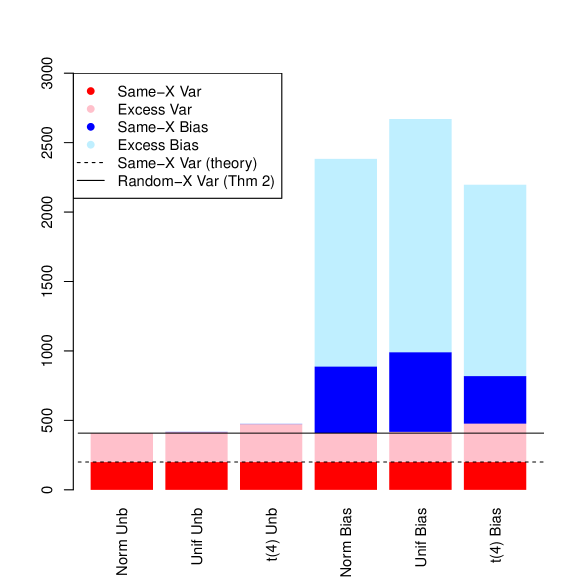
Figure 1: Decomposition of Random-X prediction error into its reducible components: Same-X bias $B$, Same-X variance $V$, excess bias $B^{+}$, and excess variance $V^{+}$, in the “high-dimensional” case with $n=100$ and $p=50$.

5.2 Comparison of performances in estimating prediction error

Next we compare the performance of the proposed criteria for estimating the Random-X prediction error of least squares over the six simulation settings. The results in Figures 2 and 3 correspond to the “high-dimensional” case with $n=100$ and $p=50$ and the “low-dimensional, extreme bias” case with $n=100$ and $p=10$, respectively. Displayed are the MSEs in estimating the Random-X prediction error, relative to OCV; also, the MSE for each method are broken down into squared bias and variance components.

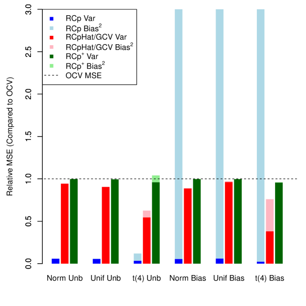
Figure 2: MSEs of the different methods in estimating Random-X prediction error relative to OCV, in the “high-dimensional” case with $n=100$ and $p=50$. The plot is truncated at a relative error of 3 for clarity, but the RCp relative errors continue as high as 10 in the biased settings.

In the high-dimensional case in Figure 2, we see that for the true linear models (three leftmost scenarios), RCp has by far the lowest MSE in estimating Random-X prediction error, much better than OCV. For the normal and uniform covariate distributions, it also has no bias in estimating this error, as warranted by Theorem 2 for the normal setting. For the $t(4)$ distribution, there is already significant bias in the prediction error estimates generated by RCp, as is expected from the results in Figure 1; however, if the linear model is correct then we see RCp still has three- to five-fold lower MSE compared to all other methods. The situation changes dramatically when bias is added (three rightmost scenarios). Now, RCp is by far the worse method, failing completely to account for large $B^{+}$, and its relative MSE compared to OCV reaches as high as 10.

As for RCp⁺ and $\widehat{{\rm RCp}}$ in the high-dimensional case, we see that RCp⁺ indeed has lower error than OCV under the normal models as argued in Section 4.4, and also in the uniform models. This is true regardless of the presence of bias. The difference, however is small: between 0.1% and 0.7%. In these settings, we can see $\widehat{{\rm RCp}}$ has even lower MSE than RCp⁺, with no evident bias in dealing with the biased models. For the long-tailed $t(4)$ distribution, both $\widehat{{\rm RCp}}$ and RCp⁺ suffer some bias in estimating prediction error, as expected. Interestingly, in the nonlinear model with $t(4)$ covariates (rightmost scenario), $\widehat{{\rm RCp}}$ does suffer significant bias in estimating prediction error, as opposed to RCp⁺. However, this bias does not offset the increased variance due to RCp⁺/OCV.

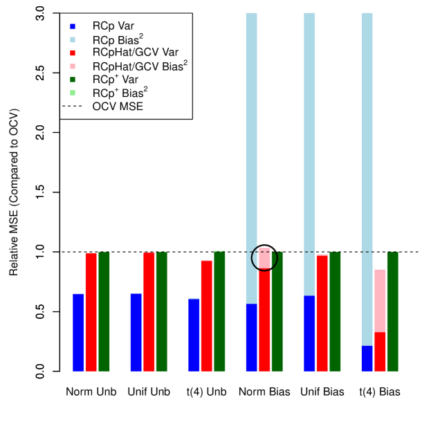
Figure 3: MSEs of the different methods in estimating Random-X prediction error relative to OCV, in the “low-dimensional, extreme bias” case with $n=100$ and $p=10$.

In the low-dimensional case in Figure 3, many of the same conclusions apply: RCp does well if the linear model is correct, even with the long-tailed covariate distribution, but fails completely in the presence of nonlinearity. Also, RCp⁺ performs almost identically to OCV throughout. The most important distinction is the failure of $\widehat{{\rm RCp}}$ in the normal covariate, biased setting, where it suffers significant bias in estimating the prediction error (see circled region in the plot). This demonstrates that the heuristic correction for $B^{+}$employed by $\widehat{{\rm RCp}}$ can fail when the linear model does not hold, as opposed to RCp⁺ and OCV. We discuss this further in Section 8.

6 The effects of ridge regularization

In this section, we examine ridge regression, which behaves similarly in some ways to least squares regression, and differently in others. In particular, like least squares, it has nonnegative excess bias, but unlike least squares, it can have negative excess variance, increasingly so for larger amounts of regularization.

These results are established in the subsections below, where we study excess bias and variance separately. Throughout, we will write $\hat{f}_{n}$ for the estimator from the ridge regression of $Y$ on $X$, i.e., $\hat{f}_{n}(x)=x^{T}(X^{T}X+\lambda I)^{-1}X^{T}Y$, where the tuning parameter $\lambda>0$ is considered arbitrary (and for simplicity, we make the dependence of $\hat{f}_{n}$ on $\lambda$ implicit). When $\lambda=0$, we must assume that $X$ has full column rank (almost surely under its marginal distribution $Q^{n}$), but when $\lambda>0$, no assumption is needed on $X$.

6.1 Nonnegativity of $B^{+}$

We prove an extension to the excess bias result in Theorem 1 for least squares regression that the excess bias in ridge regression is nonnegative.

Theorem 4.

For $\hat{f}_{n}$ the ridge regression estimator, we have $\text{$B^{+}$}\geq 0$.

Proof.

This result is actually itself a special case of Theorem 6; the latter is phrased in somewhat of a different (functional) notation, so for concreteness, we give a direct proof of the result for ridge regression here. Let $X_{0}\in\mathbb{R}^{n\times p}$ be a matrix of test covariate values, with rows i.i.d. from $Q$, and let $Y_{0}\in\mathbb{R}^{n}$ be a vector of associated test response value. Then excess bias in (4) can be written as

$$\text{$B^{+}$}=\mathbb{E}_{X,X_{0}}\frac{1}{n}\big{\|}\mathbb{E}\big{(}\hat{f}_{n}(X_{0})\,|\,X,X_{0}\big{)}-f(X_{0})\big{\|}_{2}^{2}-\mathbb{E}_{X}\frac{1}{n}\big{\|}\mathbb{E}\big{(}\hat{f}_{n}(X)\,|\,X\big{)}-f(X)\big{\|}_{2}^{2}.$$

Note $\hat{f}_{n}(X)=X(X^{T}X+\lambda I)^{-1}X^{T}Y$, and by linearity, $\mathbb{E}(\hat{f}_{n}(X)\,|\,X)=X(X^{T}X+\lambda I)^{-1}X^{T}f(X)$. Recalling the optimization problem underlying ridge regression, we thus have

$$\mathbb{E}\big{(}\hat{f}_{n}(X)\,|\,X\big{)}=\mathop{\mathrm{argmin}}_{X\beta\in\mathbb{R}^{n}}\;\|f(X)-X\beta\|_{2}^{2}+\lambda\|\beta\|_{2}^{2}.$$

An analogous statement holds for $\hat{f}_{0n}$, which we write to denote the result from the ridge regression $Y_{0}$ on $X_{0}$; we have

$$\mathbb{E}\big{(}\hat{f}_{0n}(X_{0})\,|\,X_{0}\big{)}=\mathop{\mathrm{argmin}}_{X_{0}\beta\in\mathbb{R}^{n}}\;\|f(X_{0})-X_{0}\beta\|_{2}^{2}+\lambda\|\beta\|_{2}^{2}.$$

Now write $\beta_{n}=(X^{T}X+\lambda I)^{-1}X^{T}f(X)$ and $\beta_{0n}=(X_{0}^{T}X_{0}+\lambda I)^{-1}X_{0}^{T}f(X_{0})$ for convenience. By optimality of $X_{0}\beta_{0n}$ for the minimization problem in the last display,

$$\|X_{0}\beta_{n}-f(X_{0})\|_{2}^{2}+\lambda\|\beta_{n}\|_{2}^{2}\geq\|X_{0}\beta_{0n}-f(X_{0})\|_{2}^{2}+\lambda\|\beta_{0n}\|_{2}^{2},$$

and taking an expectation over $X,X_{0}$ gives

$$\mathbb{E}_{X,X_{0}}\Big{[}\|X_{0}\beta_{n}-f(X_{0})\|_{2}^{2}+\lambda\|\beta_{n}\|_{2}^{2}\Big{]} \geq\mathbb{E}_{X_{0}}\Big{[}\|X_{0}\beta_{0n}-f(X_{0})\|_{2}^{2}+\lambda\|\beta_{0n}\|_{2}^{2}\Big{]}$$

$$=\mathbb{E}_{X}\Big{[}\|X\beta_{n}-f(X)\|_{2}^{2}+\lambda\|\beta_{n}\|_{2}^{2}\Big{]},$$

where in the last line we used the fact that $(X,Y)$ and $(X_{0},Y_{0})$ are identical in distribution. Cancelling out the common term of $\lambda\,\mathbb{E}_{X}\|\beta_{n}\|_{2}^{2}$ in the first and third lines above establishes the result, since $\mathbb{E}(\hat{f}_{n}(X_{0})\,|\,X,X_{0})=X_{0}\beta_{n}$ and $\mathbb{E}(\hat{f}_{n}(X)\,|\,X)=X\beta_{n}$. ∎

6.2 Negativity of $V^{+}$ for large $\lambda$

Here we present two complementary results on the variance side.

Proposition 2.

For $\hat{f}_{n}$ the ridge regression estimator, the integrated Random-X prediction variance,

$$V+\text{$V^{+}$}=\mathbb{E}_{X,x_{0}}\mathrm{Var}\big{(}\hat{f}_{n}(x_{0})\,|\,X,x_{0}\big{)},$$

is a nonincreasing function of $\lambda$.

Proof.

As in the proofs of Theorems 1 and 4, let $X_{0}\in\mathbb{R}^{n\times p}$ be a test covariate matrix, and notice that we can write the integrated Random-X variance as

$$V+\text{$V^{+}$}=\mathbb{E}_{X,X_{0}}\frac{1}{n}\mathrm{tr}\big{[}\mathrm{Cov}\big{(}\hat{f}_{n}(X_{0})\,|\,X,X_{0}\big{)}\big{]}.$$

For a given value of $X,X_{0}$, we have

$$\frac{1}{n}\mathrm{tr}\big{[}\mathrm{Cov}\big{(}\hat{f}_{n}(X_{0})\,|\,X,X_{0}\big{)}\big{]} =\frac{\sigma^{2}}{n}\mathrm{tr}\Big{(}X_{0}(X^{T}X+\lambda I)^{-1}X^{T}X(X^{T}X+\lambda I)^{-1}X_{0}^{T}\Big{)}$$

$$=\frac{\sigma^{2}}{n}\mathrm{tr}\bigg{(}X_{0}^{T}X_{0}\sum_{i=1}^{p}u_{i}u_{i}^{T}\frac{d_{i}^{2}}{(d_{i}^{2}+\lambda)^{2}}\bigg{)},$$

where the second line uses an eigendecomposition $X^{T}X=UDU^{T}$, with $U\in\mathbb{R}^{p\times p}$ having orthonormal columns $u_{1},\ldots,u_{p}$ and $D=\mathrm{diag}(d_{1}^{2},\ldots,d_{p}^{2})$. Taking a derivative with respect to $\lambda$, we see

$$\frac{d}{d\lambda}\Bigg{(}\frac{1}{n}\mathrm{tr}\big{[}\mathrm{Cov}\big{(}\hat{f}_{n}(X_{0})\,|\,X,X_{0}\big{)}\big{]}\Bigg{)}=-2\frac{\sigma^{2}}{n}\mathrm{tr}\bigg{(}X_{0}^{T}X_{0}\sum_{i=1}^{p}u_{i}u_{i}^{T}\frac{\lambda d_{i}^{2}}{(d_{i}^{2}+\lambda)^{3}}\bigg{)}\leq 0,$$

the inequality due to the fact that $\mathrm{tr}(AB)\geq 0$ if $A,B$ are positive semidefinite matrices. Taking an expectation and switching the order of integration and differentiation (which is possible because the integrand is a continuously differentiable function of $\lambda>0$) gives

$$\frac{d}{d\lambda}\Bigg{(}\mathbb{E}_{X,X_{0}}\frac{1}{n}\mathrm{tr}\big{[}\mathrm{Cov}\big{(}\hat{f}_{n}(X_{0})\,|\,X,X_{0}\big{)}\big{]}\Bigg{)}=\mathbb{E}_{X,X_{0}}\frac{d}{d\lambda}\Bigg{(}\frac{1}{n}\mathrm{tr}\big{[}\mathrm{Cov}\big{(}\hat{f}_{n}(X_{0})\,|\,X,X_{0}\big{)}\big{]}\Bigg{)}\leq 0,$$

the desired result. ∎

The proposition shows that adding regularization guarantees a decrease in variance for Random-X prediction. The same is true of the variance in Same-X prediction. However, as we show next, as the amount of regularization increases these two variances decrease at different rates, a phenomenon that manifests itself in the fact that and the Random-X prediction variance is guaranteed to be smaller than the Same-X prediction variance for large enough $\lambda$.

Theorem 5.

For $\hat{f}_{n}$ the ridge regression estimator, the integrated Same-X prediction variance and integrated Random-X prediction variance both approach zero as $\lambda\to\infty$. Moreover, the limit of their ratio satisfies

$$\lim_{\lambda\to\infty}\frac{\mathbb{E}_{X,x_{0}}\mathrm{Var}(\hat{f}_{n}(x_{0})\,|\,X,x_{0})}{\mathbb{E}_{X}\mathrm{Var}(\hat{f}_{n}(x_{1})\,|\,X)}=\frac{\mathrm{tr}[\mathbb{E}(X^{T}X)\mathbb{E}(X^{T}X)]}{\mathrm{tr}[\mathbb{E}(X^{T}XX^{T}X)]}\leq 1,$$

the last inequality reducing to an equality if and only if $x\sim Q$ is deterministic and has no variance.

Proof.

Again, as in the proof of the last proposition as well as Theorems 1 and 4, let $X_{0}\in\mathbb{R}^{n\times p}$ be a test covariate matrix, and write the integrated Same-X and Random-X prediction variances as

$$\mathbb{E}_{X}\frac{1}{n}\mathrm{tr}\big{[}\mathrm{Cov}\big{(}\hat{f}_{n}(X)\,|\,X\big{)}\big{]}\quad\text{and}\quad\mathbb{E}_{X,X_{0}}\frac{1}{n}\mathrm{tr}\big{[}\mathrm{Cov}\big{(}\hat{f}_{n}(X_{0})\,|\,X,X_{0}\big{)}\big{]},$$

respectively. From the arguments in the proof of Proposition 2, letting $X^{T}X=UDU^{T}$ be an eigendecomposition with $U\in\mathbb{R}^{p\times p}$ having orthonormal columns $u_{1},\ldots,u_{p}$ and $D=\mathrm{diag}(d_{1}^{2},\ldots,d_{p}^{2})$, we have

$$\lim_{\lambda\to\infty}\mathbb{E}_{X,X_{0}}\frac{1}{n}\mathrm{tr}\big{[}\mathrm{Cov}\big{(}\hat{f}_{n}(X_{0})\,|\,X,X_{0}\big{)}\big{]} =\lim_{\lambda\to\infty}\mathbb{E}_{X,X_{0}}\frac{\sigma^{2}}{n}\mathrm{tr}\bigg{(}X_{0}^{T}X_{0}\sum_{i=1}^{p}u_{i}u_{i}^{T}\frac{d_{i}^{2}}{(d_{i}^{2}+\lambda)^{2}}\bigg{)}$$

$$=\mathbb{E}_{X,X_{0}}\lim_{\lambda\to\infty}\frac{\sigma^{2}}{n}\mathrm{tr}\bigg{(}X_{0}^{T}X_{0}\sum_{i=1}^{p}u_{i}u_{i}^{T}\frac{d_{i}^{2}}{(d_{i}^{2}+\lambda)^{2}}\bigg{)}=0,$$

where in the second line we used the dominated convergence theorem to exchange the limit and the expectation (since $\mathbb{E}_{X,X_{0}}\mathrm{tr}[X_{0}^{T}X_{0}\sum_{i=1}^{p}u_{i}u_{i}^{T}(d_{i}^{2}/(d_{i}^{2}+\lambda)^{2})]\leq\mathbb{E}_{X,X_{0}}\mathrm{tr}(X_{0}^{T}X_{0}X^{T}X)<\infty$). Similar arguments show that the integrated Same-X prediction variance also tends to zero.

Now we consider the limiting ratio of the integrated variances,

$$\lim_{\lambda\to\infty}\frac{\mathbb{E}_{X,X_{0}}\mathrm{tr}[\mathrm{Cov}(\hat{f}_{n}(X_{0})\,|\,X,X_{0})]}{\mathbb{E}_{X}\mathrm{tr}[\mathrm{Cov}(\hat{f}_{n}(X)\,|\,X)]} =\lim_{\lambda\to\infty}\frac{\mathbb{E}_{X,X_{0}}\mathrm{tr}[X_{0}(X^{T}X+\lambda I)^{-1}X^{T}X(X^{T}X+\lambda I)^{-1}X_{0}^{T}]}{\mathbb{E}_{X}\mathrm{tr}[X(X^{T}X+\lambda I)^{-1}X^{T}X(X^{T}X+\lambda I)^{-1}X^{T}]}$$

$$=\lim_{\lambda\to\infty}\frac{\mathbb{E}_{X,X_{0}}\mathrm{tr}[\lambda^{2}X_{0}(X^{T}X+\lambda I)^{-1}X^{T}X(X^{T}X+\lambda I)^{-1}X_{0}^{T}]}{\mathbb{E}_{X}\mathrm{tr}[\lambda^{2}X(X^{T}X+\lambda I)^{-1}X^{T}X(X^{T}X+\lambda I)^{-1}X^{T}]}$$

$$=\frac{\lim_{\lambda\to\infty}\mathbb{E}_{X,X_{0}}\mathrm{tr}[\lambda^{2}X_{0}(X^{T}X+\lambda I)^{-1}X^{T}X(X^{T}X+\lambda I)^{-1}X_{0}^{T}]}{\lim_{\lambda\to\infty}\mathbb{E}_{X}\mathrm{tr}[\lambda^{2}X(X^{T}X+\lambda I)^{-1}X^{T}X(X^{T}X+\lambda I)^{-1}X^{T}]},$$

where the last line holds provided that the numerator and denominator both converge to finite nonzero limits, as will be confirmed by our arguments below. We study the numerator first. Noting that $\lambda^{2}(X^{T}X+\lambda I)^{-1}X^{T}X(X^{T}X+\lambda I)^{-1}-X^{T}X$ has eigenvalues

$$d_{i}^{2}\bigg{(}\frac{\lambda^{2}}{(d_{i}^{2}+\lambda)^{2}}-1\bigg{)},\;i=1,\ldots,p,$$

we have that $\lambda^{2}(X^{T}X+\lambda I)^{-1}X^{T}X(X^{T}X+\lambda I)^{-1}\to X^{T}X$ as $\lambda\to\infty$, in (say) the operator norm, implying $\mathrm{tr}[\lambda^{2}X_{0}(X^{T}X+\lambda I)^{-1}X^{T}X(X^{T}X+\lambda I)^{-1}X_{0}^{T}]\to\mathrm{tr}(X_{0}X^{T}XX_{0}^{T})$ as $\lambda\to\infty$. Hence

$$\lim_{\lambda\to\infty}\mathbb{E}_{X,X_{0}}\mathrm{tr}\big{[}\lambda^{2}X_{0}(X^{T}X+\lambda I)^{-1} X^{T}X(X^{T}X+\lambda I)^{-1}X_{0}^{T}\big{]}$$

$$=\mathbb{E}_{X,X_{0}}\lim_{\lambda\to\infty}\mathrm{tr}\big{[}\lambda^{2}X_{0}(X^{T}X+\lambda I)^{-1}X^{T}X(X^{T}X+\lambda I)^{-1}X_{0}^{T}\big{]}$$

$$=\mathbb{E}_{X,X_{0}}\mathrm{tr}(X_{0}X^{T}XX_{0}^{T})$$

$$=\mathrm{tr}\big{[}\mathbb{E}_{X}(X^{T}X)\mathbb{E}_{X_{0}}(X_{0}^{T}X_{0})\big{]}$$

$$=\mathrm{tr}\big{[}\mathbb{E}_{X}(X^{T}X)\mathbb{E}_{X}(X^{T}X)\big{]}.$$

Here, in the first line, we applied the dominated convergence theorem as previously, in the third we used the independence of $X,X_{0}$, and in the last we used the identical distribution of $X,X_{0}$. Similar arguments lead to the conclusion for the denominator

$$\lim_{\lambda\to\infty}\mathbb{E}_{X}\mathrm{tr}\big{[}\lambda^{2}X(X^{T}X+\lambda I)^{-1}X^{T}X(X^{T}X+\lambda I)^{-1}X^{T}\big{]}=\mathrm{tr}\big{[}\mathbb{E}_{X}(X^{T}XX^{T}X)\big{]},$$

and thus we have shown that

$$\lim_{\lambda\to\infty}\frac{\mathbb{E}_{X,X_{0}}\mathrm{tr}[\mathrm{Cov}(\hat{f}_{n}(X_{0})\,|\,X,X_{0})]}{\mathbb{E}_{X}\mathrm{tr}[\mathrm{Cov}(\hat{f}_{n}(X)\,|\,X)]}=\frac{\mathrm{tr}[\mathbb{E}_{X}(X^{T}X)\mathbb{E}_{X}(X^{T}X)]}{\mathrm{tr}[\mathbb{E}_{X}(X^{T}XX^{T}X)]},$$

as desired. To see that the ratio on the right-hand side is at most 1, consider

$$A=\mathbb{E}(X^{T}XX^{T}X)-\mathbb{E}(X^{T}X)\mathbb{E}(X^{T}X),$$

which is a symmetric matrix whose trace is

$$\mathrm{tr}(A)=\sum_{i,j=1}^{p}\mathrm{Var}\big{(}(X^{T}X)_{i,j}\big{)}\geq 0.$$

Furthermore, the trace is zero if and only if all summands are zero, which occurs if and only if all components of $x\sim Q$ have no variance. ∎

In words, the theorem shows that the excess variance $V^{+}$ of ridge regression approaches zero as $\lambda\to\infty$, but it does so from the left (negative side) of zero. As we can have cases in which the excess bias is very small or even zero (for example, a null model like in our simulations below), we see that ${\rm ErrR}-{\rm ErrS}=\text{$V^{+}$}$ can be negative for ridge regression with a large level of regularization; this is a striking contrast to the behavior of this gap for least squares, where it is always nonnegative.

We finish by demonstrating this result empirically, using a simple simulation setup with $p=100$ covariates drawn from $Q=N(0,I)$, and training and test sets each of size $n=300$. The underlying regression function was $f(x)=\mathbb{E}(y|x)=0$, i.e., there was no signal, and the errors were also standard normal. We drew training and test data from this simulation setup, fit ridge regression estimators to the training at various levels of $\lambda$, and calculated the ratio of the sample versions of the Random-X and Same-X integrated variances. We repeated this 100 times, and averaged the results. As shown in Figure 4, for values of $\lambda$ larger than about 250, the Random-X integrated variance is smaller than the Same-X integrated variance, and consequently the same is true of the prediction errors (as there is no signal, the Same-X and Random-X integrated biases are both zero). Also shown in the figure is the theoretical limiting ratio of the integrated variances according to Theorem 5, which in this case can be calculated from the properties of Wishart distributions to be $n^{2}p/(n^{2}p+np^{2}+np)\approx 0.7481$, and is in very good agreement with the empirical limiting ratio.

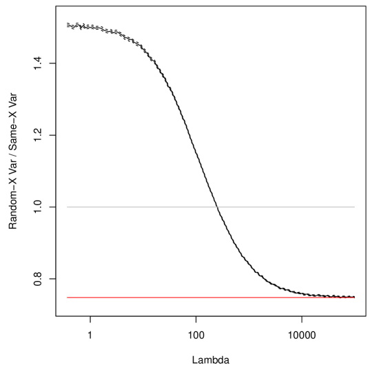
Figure 4: Ratio of Random-X integrated variance to Same-X integrated variance for ridge regression as we vary the tuning parameter $\lambda$, in a simple problem setting with $p=100$ covariates and training and test sets each of size $n=300$. For values of $\lambda$ larger than about 250, the ratio is smaller than 1, meaning the Random-X prediction variance is smaller than the Same-X prediction variance; as the integrated bias is zero in both settings, the same ordering also applies to the Random-X and Same-X prediction errors. The plotted curve is an average of the computed ratios over 100 repetitions, and the dashed lines (hard to see, because they are very close to the aforementioned curve) denote 95% confidence intervals over these repetitions. The red line is the theoretical limiting ratio of integrated variances due to Theorem 5, in good agreement with the simulation results.

7 Nonparametric regression estimators

We present a brief study of the excess bias and variance of some common nonparametric regression estimators. In Section 8, we give a high-level discussion of the view on the gap between Random-X and Same-X prediction errors from the perspective of empirical process theory, which is a topic that is well-studied by researchers in nonparametric regression.

7.1 Reproducing kernel Hilbert spaces

Consider an estimator $\hat{f}_{n}$ defined by the general-form functional optimization problem

$$\hat{f}_{n}=\mathop{\mathrm{argmin}}_{g\in\mathcal{G}}\;\sum_{i=1}^{n}\big{(}y_{i}-g(x_{i})\big{)}^{2}+J(g),$$ (9)

where $\mathcal{G}$ is a function class and $J$ is a roughness penalty on functions. Examples estimators of this form include the (cubic) smoothing spline estimator in $p=1$ dimensions, in which $\mathcal{G}$ is the space of all functions that are twice differentiable and whose second derivative is in square integrable, and $J(g)=\int g^{\prime\prime}(t)^{2}\,dt$; and more broadly, reproducing kernel Hilbert space or RKHS estimators (in an arbitrary dimension $p$), in which $\mathcal{G}$ is an RKHS and $J(g)=\|f\|_{\mathcal{G}}$ is the corresponding RKHS norm.

Provided that $\hat{f}_{n}$ defined by (9) is a linear smoother, which means $\hat{f}_{n}(x)=s(x)^{T}Y$ for a weight function $s:\mathbb{R}^{p}\to\mathbb{R}$ (that can and will generally also depend on $X$), we now show that the excess bias of $\hat{f}_{n}$ is always nonnegative. We note that this result applies to smoothing splines and RKHS estimators, since these are linear smoothers; it also covers ridge regression, and thus generalizes the result in Theorem 4.

Theorem 6.

For $\hat{f}_{n}$ a linear smoother defined by a problem of the form (9), we have $\text{$B^{+}$}\geq 0$.

Proof.

Let us introduce a test covariate matrix $X_{0}\in\mathbb{R}^{n\times p}$ and associated response vector $Y_{0}\in\mathbb{R}^{n}$, and write the excess bias in (4) as

$$\text{$B^{+}$}=\mathbb{E}_{X,X_{0}}\frac{1}{n}\big{\|}\mathbb{E}\big{(}\hat{f}_{n}(X_{0})\,|\,X,X_{0}\big{)}-f(X_{0})\big{\|}_{2}^{2}-\mathbb{E}_{X}\frac{1}{n}\big{\|}\mathbb{E}\big{(}\hat{f}_{n}(X)\,|\,X\big{)}-f(X)\big{\|}_{2}^{2}.$$

Writing $\hat{f}_{n}(x)=s(x)^{T}Y$ for a weight function $s:\mathbb{R}^{p}\to\mathbb{R}$, let $S(X)\in\mathbb{R}^{n\times n}$ be a smoother matrix that has rows $s(x_{1}),\ldots,s(x_{n})$. Thus $\hat{f}_{n}(X)=S(X)Y$, and by linearity, $\mathbb{E}(\hat{f}_{n}(X)\,|\,X)=S(X)f(X)$. This in fact means that we can express $g_{n}=\mathbb{E}(\hat{f}_{n}|X)$, a function defined by $g(x)=s(x)^{T}f(X)$, as the solution of an optimization problem of the form (9),

$$g_{n}=\mathop{\mathrm{argmin}}_{g\in\mathcal{G}}\;\|f(X)-g(X)\|_{2}^{2}+J(g),$$

where we have rewritten the loss term in a more convenient notation. Analogously, if we denote by $\hat{f}_{0n}$ the estimator of the form (9), but fit to the test data $X_{0},Y_{0}$ instead of the training data $X,Y$, and $g_{0n}=\mathbb{E}(\hat{f}_{0n}|X_{0})$, then

$$g_{0n}=\mathop{\mathrm{argmin}}_{g\in\mathcal{G}}\;\|f(X_{0})-g(X_{0})\|_{2}^{2}+J(g).$$

By virtue of optimality of $g_{0n}$ for the problem in the last display, we have

$$\|g_{n}(X_{0})-f(X_{0})\|_{2}^{2}+J(g_{n})\geq\|g_{0n}(X_{0})-f(X_{0})\|_{2}^{2}+J(g_{0n})$$

and taking an expectation over $X,X_{0}$ gives

$$\mathbb{E}_{X,X_{0}}\Big{[}\|g_{n}(X_{0})-f(X_{0})\|_{2}^{2}+J(g_{n})\Big{]} \geq\mathbb{E}_{X_{0}}\Big{[}\|g_{0n}(X_{0})-f(X_{0})\|_{2}^{2}+J(g_{0n})\Big{]}$$

$$=\mathbb{E}_{X}\Big{[}\|g_{n}(X)-f(X)\|_{2}^{2}+J(g_{n})\Big{]},$$

where in the equality step we used the fact that $X,X_{0}$ are identical in distribution. Cancelling out the common term of $\mathbb{E}_{X}J(g_{n})$ from the the first and third expressions proves the result, because $\mathbb{E}(\hat{f}_{n}(X_{0})\,|\,X,X_{0})=g_{n}(X_{0})$ and $\mathbb{E}(\hat{f}_{n}(X)\,|\,X)=g_{n}(X)$. ∎

7.2 $k$-nearest-neighbors regression

Consider $\hat{f}_{n}$ the $k$-nearest-neighbors or kNN regression estimator, defined by

$$\hat{f}_{n}(x)=\frac{1}{k}\sum_{i\in N_{k}(x)}y_{i},$$

where $N_{k}(x)$ returns the indices of the $k$ nearest points among $x_{1},\ldots,x_{n}$ to $x$. It is immediate that the excess variance of kNN regression is zero.

Proposition 3.

For $\hat{f}_{n}$ the kNN regression estimator, we have $\text{$V^{+}$}=0$.

Proof.

Simply compute

$$\mathrm{Var}\big{(}\hat{f}_{n}(x_{1})\,|X\big{)}=\frac{\sigma^{2}}{k},$$

by independence of $y_{1},\ldots,y_{n}$, and hence the points in the nearest neighbor set $N_{k}(x_{1})$, conditional on $X$. Similarly,

$$\mathrm{Var}\big{(}\hat{f}_{n}(x_{0})\,|X,x_{0}\big{)}=\frac{\sigma^{2}}{k}.$$

∎

On the other hand, the excess bias is not easily computable, and is not covered by Theorem 6, since kNN cannot be written as an estimator of the form (9) (though it is a linear smoother). The next result sheds some light on the nature of the excess bias.

Proposition 4.

For $\hat{f}_{n}$ the kNN regression estimator, we have

$$\text{$B^{+}$}=B_{n,k}-\bigg{(}1-\frac{1}{k^{2}}\bigg{)}B_{n-1,k-1},$$

where $B_{n,k}$ denotes the integrated Random-X prediction bias of the kNN estimator fit to a training set of size $n$, and with tuning parameter (number of neighbors) $k$.

Proof.

Observe

$$\Big{(}\mathbb{E}\big{(}\hat{f}_{n}(x_{0})\,|\,X,x_{0}\big{)}-f(x_{0})\Big{)}^{2}=\Bigg{(}\frac{1}{k}\sum_{i\in N_{k}(x_{0})}\big{(}f(x_{i})-f(x_{0})\big{)}\Bigg{)}^{2},$$

and by definition, $\mathbb{E}_{X,x_{0}}[\mathbb{E}(\hat{f}_{n}(x_{0})\,|\,X,x_{0})-f(x_{0})]^{2}=B_{n,k}$. Meanwhile

$$\Big{(}\mathbb{E}\big{(}\hat{f}_{n}(x_{1})\,|\,X\big{)}-f(x_{1})\Big{)}^{2}=\Bigg{(}\frac{1}{k}\sum_{i\in N_{k}(x_{1})}\big{(}f(x_{i})-f(x_{1})\big{)}\Bigg{)}^{2}=\Bigg{(}\frac{1}{k}\sum_{i\in N_{k}^{-1}(x_{1})}\big{(}f(x_{i})-f(x_{1})\big{)}\Bigg{)}^{2},$$

where $N_{k-1}^{-1}(x_{1})$ gives the indices of the $k-1$ nearest points among $x_{2},\ldots,x_{n}$ to $x_{1}$ (which equals $N_{k}(x_{1})$ as $x_{1}$ is trivially one of its own $k$ nearest neighbors). Now notice that $x_{1}$ plays the role of the test point $x_{0}$ in the last display, and therefore, $\mathbb{E}_{X}[\mathbb{E}(\hat{f}_{n}(x_{1})\,|\,X)-f(x_{1})]^{2}=((k-1)/k)^{2}B_{n-1,k-1}$. This proves the result. ∎

The above proposition suggests that, for moderate values of $k$, the excess bias in kNN regression is likely positive. We are comparing the integrated Random-X bias of a kNN model with $n$ training points and $k$ neighbors to that of a model $n-1$ points and $k-1$ neighbors; for large $n$ and moderate $k$, it seems that the former should be larger than the latter, and in addition, the factor of $(1-1/k^{2})$ multiplying the latter term makes it even more likely that the difference $B_{n,k}-(1-1/k^{2})B_{n-1,k-1}$ is positive. Rephrased, using the zero excess variance result of Proposition 3: the gap in Random-X and Same-X prediction errors, ${\rm ErrR}-{\rm ErrS}=B_{n,k}-(1-1/k^{2})B_{n-1,k-1}$, is likely positive for large $n$ and moderate $k$. Of course, this is not a formal proof; aside from the choice of $k$, the shape of the underlying mean function $f(x)=\mathbb{E}(y|x)$ obviously plays an important role here too. As a concrete problem setting, we might try analyzing the Random-X bias $B_{n,k}$ for $f$ Lipschitz and a scaling for $k$ such that $k\to\infty$ but $k/n\to 0$ as $n\to\infty$, e.g., $k\asymp\sqrt{n}$, which ensures consistency of kNN. Typical analyses provide upper bounds on the kNN bias in this problem setting (e.g., see Gyorfi et al. 2002), but a more refined analysis would be needed to compare $B_{n,k}$ to $B_{n-1,k-1}$.

8 Discussion

We have proposed and studied a division of Random-X prediction error into components: the irreducible error $\sigma^{2}$, the traditional (Fixed-X or Same-X) integrated bias $B$ and integrated variance $V$ components, and our newly defined excess bias $B^{+}$ and excess variance $V^{+}$ components, such that $B+\text{$B^{+}$}$ gives the Random-X integrated bias and $V+\text{$V^{+}$}$ the Random-X integrated variance. For least squares regression, we were able to quantify $V^{+}$ exactly when the covariates are normal and asymptotically when they are drawn from a linear transformation of a product distribution, leading to our definition of RCp. To account for unknown error variance $\sigma^{2}$, we defined $\widehat{{\rm RCp}}$ based on the usual plug-in estimate, which turns out to be asymptotically identical to GCV, giving this classic method a novel interpretation. To account for $B^{+}$ (when $\sigma^{2}$ is known and the distribution $Q$ of the covariates is well-behaved), we defined RCp⁺, by leveraging a Random-X bias estimate implicit to OCV. We also briefly considered methods beyond least squares, proving that $B^{+}$ is nonnegative in all settings considered, while $V^{+}$ can become negative in the presence of heavy regularization.

We reflect on some issues surrounding our findings and possible directions for future work.

Ability of $\widehat{{\rm RCp}}$ to account for bias.

An intriguing phenomenon that we observe is the ability of $\widehat{{\rm RCp}}$/Sp and its close (asymptotic) relative GCV to deal to some extent with $B^{+}$ in estimating Random-X prediction error, through the inflation it performs on the squared training residuals. For GCV in particular, where recall $\mathrm{GCV}=\mathrm{RSS}/(n(1-\gamma)^{2})$, we see that this inflation a simple form: if the linear model is biased, then the squared bias component in each residual is inflated by $1/(1-\gamma)^{2}$. Comparing this to the inflation that OCV performs, which is $1/(1-h_{ii})^{2}$, on the $i$th residual, for $i=1,\ldots,n$, we can interpret GCV as inflating the bias for each residual by some “averaged” version of the elementwise factors used by OCV. As OCV provides an almost-unbiased estimate of $B^{+}$ for Random-X prediction, GCV can get close when the diagonal elements $h_{ii}$, $i=1,\ldots,n$ do not vary too wildly. When they do vary greatly, GCV can fail to account for $B^{+}$, as in the circled region in Figure 3.

Alternative bias-variance decompositions.

The integrated terms we defined are expectations of conditional bias and variance terms, where we conditioned on both training and testing covariates $X,x_{0}$. One could also consider other conditioning schemes, leading to different decompositions. An interesting option would be to condition on the prediction point $x_{0}$ only and calculate the bias and variance unconditional on the training points $X$ before integrating, as in $\mathbb{E}_{x_{0}}(\mathbb{E}(\hat{f}_{n}(x_{0})\,|\,x_{0})-f(x_{0}))^{2}$ and $\mathbb{E}_{x_{0}}(\mathrm{Var}(\hat{f}_{n}(x_{0})\,|\,x_{0}))$ for these alternative notions of Random-X bias and variance, respectively. It is easy to see that this would cause the bias (and thus excess bias) to decrease and variance (and thus excess variance) to increase. However, it is not clear to us that computing or bounding such new definitions of (excess) bias and (excess) variance would be possible even for least squares regression. Investigating the tractability of this approach and any insights it might offer is an interesting topic for future study.

Alternative definitions of prediction error.

The overall goal in our work was to estimate the prediction error, defined as ${\rm ErrR}=\mathbb{E}_{X,Y,x_{0},y_{0}}(y_{0}-\hat{f}_{n}(x_{0}))^{2}$, the squared error integrated over all of the random variables available in training and testing. Alternative definitions have been suggested by some authors. Breiman and Spector (1992) generalized the Fixed-X setting in a manner that led them to define $\mathbb{E}_{Y,x_{0},y_{0}}[(y_{0}-\hat{f}_{n}(x_{0}))^{2}\,|\,X]$ as the prediction error quantity of interest, which can be interpreted as the Random-X prediction error of a Fixed-X model. Hastie et al. (2009) emphasized the importance of the quantity $\mathbb{E}_{x_{0},y_{0}}[(y_{0}-\hat{f}_{n}(x_{0}))^{2}\,|\,X,Y]$, which is the out-of-sample error of the specific model we have trained on the given training data $X,Y$. Of these two alternate definitions, the second one is more interesting in our opinion, but investigating it rigorously requires a different approach than what we have developed here.

Alternative types of cross-validation.

Our exposition has concentrated on comparing OCV to generalized covariance penalty methods. We have not discussed other cross-validation approaches, in particular, K-fold cross-validation (KCV) method with $K\ll n$ (e.g., $K=5$ or 10). A supposedly well-known problem with OCV is that its estimates of prediction error have very high variance; we indeed observe this phenomenon in our simulations (and for least squares estimation, the analytical form of OCV clarifies the source of this high variance). There are some claims in the literature that KCV can have lower variance than OCV (Hastie et al. 2009, and others), and should be considered as the preferred CV variant for estimation of Random-X prediction error. Systematic investigations of this issue for least squares regression such as Burman (1989); Arlot and Celisse (2010) actually reach the opposite conclusion—that high variance is further compounded by reducing $K$. Our own simulations also support this view (results not shown), therefore we do not consider KCV to be an important benchmark to consider beyond OCV.

Model selection for prediction.

Our analysis and simulations have focused on the accuracy of prediction error estimates provided by various approaches. We have not considered their utility for model selection, i.e., for identifying the best predictive model, which differs from model evaluation in an important way. A method can do well in the model selection task even when it is inaccurate or biased for model evaluation, as long as such inaccuracies are consistent across different models and do not affect its ability to select the better predictive model. Hence the correlation of model evaluations using the same training data across different models plays a central role in model selection performance. An investigation of the correlation between model evaluations that each of the approaches we considered here creates is of major interest, and is left to future work.

Semi-supervised settings.

Given the important role that the marginal distribution $Q$ of $x$ plays in evaluating Random-X prediction error (as expressed, e.g., in Theorems 2 and 3), it is of interest to consider situations where, in addition to the training data, we have large quantities of additional observations with $x$ only and no response $y$. In the machine learning literature this situation is often considered under then names semi-supervised learning or transductive learning. Such data could be used, e.g., to directly estimate the excess variance from expressions like (7).

General view from empirical process theory.

This paper was focused in large part on estimating or bounding the excess bias and variance in specific problem settings, which led to estimates or bounds on the gap in Random-X and Same-X prediction error, as ${\rm ErrR}-{\rm Err}=\text{$B^{+}$}+\text{$V^{+}$}$. This gap is indeed a familiar concept to those well-versed in the theory of nonparametric regression, and roughly speaking, standard results from empirical process theory suggest that we should in general expect ${\rm ErrR}-{\rm ErrS}$ to be small, i.e., much smaller than either of ErrR or ErrS to begin with. The connection is as follows. Note that

$${\rm ErrR}-{\rm ErrS} =\mathbb{E}_{X,Y,x_{0}}\big{(}f(x_{0})-\hat{f}_{n}(x_{0})\big{)}^{2}-\mathbb{E}_{X,Y}\bigg{[}\frac{1}{n}\sum_{i=1}^{n}\big{(}f(x_{i})-\hat{f}_{n}(x_{i})\big{)}^{2}\bigg{]}$$

$$=\mathbb{E}_{X,Y}\Big{[}\|f-\hat{f}_{n}\|_{L_{2}(Q)}^{2}-\|f-\hat{f}_{n}\|_{L_{2}(Q_{n})}^{2}\Big{]},$$

where we are using standard notation from nonparametric regression for “population” and “empirical” norms, $\|\cdot\|_{L_{2}(Q)}$ and $\|\cdot\|_{L_{2}(Q_{n})}$, respectively. For an appropriate function class $\mathcal{G}$, empirical process theory can be used to control the deviations between $\|g\|_{L_{2}(Q)}$ and $\|g\|_{L_{2}(Q_{n})}$, uniformly over all functions $g\in\mathcal{G}$. Such uniformity is important, because it gives us control on the difference in population and empirical norms for the (random) function $g=f-\hat{f}_{n}$ (provided of course this function lies in $\mathcal{G}$). This theory applies to finite-dimensional $\mathcal{G}$ (e.g., linear functions, which would be relevant to the case when $f$ is assumed to be linear and $\hat{f}_{n}$ is chosen to be linear), and even to infinite-dimensional classes $\mathcal{G}$, provided we have some understanding of the entropy or Rademacher complexity of $\mathcal{G}$ (e.g., this is true of Lipschitz functions, which would be relevant to the analysis of $k$-nearest-neighbors regression or kernel estimators).

Under appropriate conditions, we typically find $\mathbb{E}_{X,Y}|\|f-\hat{f}_{n}\|_{L_{2}(Q)}^{2}-\|f-\hat{f}_{n}\|_{L_{2}(Q_{n})}^{2}|=O(C_{n})$, where $C_{n}$ is the $L_{2}(Q)$ convergence rate of $\hat{f}_{n}$ to $f$. This is even true in an asymptotic setting in which $p$ grows with $n$ (so $C_{n}$ here gets replaced by $C_{n,p}$), but such high-dimensional results usually require more restrictions on the distribution $Q$ of covariates. The takeaway message: in most cases where $\hat{f}_{n}$ is consistent with rate $C_{n}$, we should expect to see the gap being ${\rm ErrR}-{\rm ErrS}=O(C_{n})$, whereas ${\rm ErrR},{\rm ErrS}\geq\sigma^{2}$, so the difference in Same-X and Random-X prediction error is quite small (as small as the Same-X and Random-X risk) compared to these prediction errors themselves; said differently, we should expect to see $\text{$B^{+}$},\text{$V^{+}$}$ being of the same order (or smaller than) $B,V$.

It is worth pointing out that several interesting aspects of our study really lie outside what can be inferred from empirical process theory. One aspect to mention is the precision of the results: in some settings we can characterize $\text{$B^{+}$},\text{$V^{+}$}$ individually, but (as described above), empirical process theory would only provide a handle on their sum. Moreover, for least squares regression estimators, with $p/n$ converging to a nonzero constant, we are able to characterize the exact asymptotic excess variance under some conditions on $Q$ (essentially, requiring $Q$ to be something like a rotation of a product distribution), in Theorem 3; note that this is a problem setting in which least squares is not consistent, and could not be treated by standard results empirical process theory.

Lastly, empirical process theory tells us nothing about the sign of

$$\|f-\hat{f}_{n}\|_{L_{2}(Q)}^{2}-\|f-\hat{f}_{n}\|_{L_{2}(Q_{n})}^{2},$$

or its expectation under $P$ (which equals ${\rm ErrR}-{\rm ErrS}=\text{$B^{+}$}+\text{$V^{+}$}$, as described above). This 1-bit quantity is of interest to us, since it tells us if the Same-X (in-sample) prediction error is optimistic compared to the Random-X (out-of-sample) prediction error. Theorems 1, 4, 5, 6 and Propositions 3, 4 all pertain to this quantity.

References

- Akaike (1973) Hirotogu Akaike. Information theory and an extension of the maximum likelihood principle. Second International Symposium on Information Theory, pages 267–281, 1973.
- Arlot and Celisse (2010) Sylvain Arlot and Alain Celisse. A survey of cross-validation procedures for model selection. Statistics Surveys, 4:40–79, 2010.
- Breiman and Freedman (1983) Leo Breiman and David Freedman. How many variables should be entered in a regression equation? Journal of the American Statistical Association, 78(381):131–136, 1983.
- Breiman and Spector (1992) Leo Breiman and Philip Spector. Submodel selection and evaluation in regression. The x-random case. International Statistical Review, 60(3):291–319, 1992.
- Buja et al. (2014) Andreas Buja, Richard Berk, Lawrence Brown, Edward George, Emil Pitkin, Mikhail Traskin, Linda Zhao, and Kai Zhang. Models as approximations, Part I: A conspiracy of nonlinearity and random regressors in linear regression. arXiv: 1404.1578, 2014.
- Buja et al. (2016) Andreas Buja, Richard Berk, Lawrence Brown, Ed George, Arun Kumar Kuchibhotla, and Linda Zhao. Models as approximations, Part II: A general theory of model-robust regression. arXiv: 1612.03257, 2016.
- Burman (1989) Prabir Burman. A comparative study of ordinary cross-validation, v-fold cross-validation and the repeated learning-testing methods. Biometrika, 76(3):503–514, 1989.
- Chatterjee (2013) Sourav Chatterjee. Assumptionless consistency of the lasso. arXiv: 1303.5817, 2013.
- Craven and Wahba (1978) Peter Craven and Grace Wahba. Smoothing noisy data with spline functions. Numerische Mathematik, 31(4):377–403, 1978.
- Dicker (2013) Lee H. Dicker. Optimal equivariant prediction for high-dimensional linear models with arbitrary predictor covariance. Electronic Journal of Statistics, 7:1806–1834, 2013.
- Dobriban and Wager (2015) Edgar Dobriban and Stefan Wager. High-dimensional asymptotics of prediction: Ridge regression and classification. arXiv: 1507.03003, 2015.
- Efron (1986) Bradley Efron. How biased is the apparent error rate of a prediction rule? Journal of the American Statistical Association, 81(394):461–470, 1986.
- Efron (2004) Bradley Efron. The estimation of prediction error: Covariance penalties and cross-validation. Journal of the American Statistical Association, 99(467):619–632, 2004.
- El Karoui (2009) Noureddine El Karoui. Concentration of measure and spectra of random matrices: Applications to correlation matrices, elliptical distributions and beyond. The Annals of Applied Probability, 19(6):2362–2405, 12 2009.
- Golub et al. (1979) Gene H Golub, Michael Heath, and Grace Wahba. Generalized cross-validation as a method for choosing a good ridge parameter. Technometrics, 21(2):215–223, 1979.
- Greenshtein and Ritov (2004) Eitan Greenshtein and Ya’acov Ritov. Persistence in high-dimensional linear predictor selection and the virtue of overparametrization. Bernoulli, 10(6):971–988, 2004.
- Groves and Rothenberg (1969) Theodore Groves and Thomas Rothenberg. A note on the expected value of an inverse matrix. Biometrika, 56(3):690–691, 1969.
- Gyorfi et al. (2002) Laszlo Gyorfi, Michael Kohler, Adam Krzyzak, and Harro Walk. A Distribution-Free Theory of Nonparametric Regression. Springer, 2002.
- Hastie et al. (2009) Trevor Hastie, Robert Tibshirani, and Jerome Friedman. The Elements of Statistical Learning; Data Mining, Inference and Prediction. Springer, 2009. Second edition.
- Hocking (1976) Ronald R. Hocking. The analysis and selection of variables in linear regression. Biometrics, 32(1):1–49, 1976.
- Hsu et al. (2014) Daniel Hsu, Sham Kakade, and Tong Zhang. Random design analysis of ridge regression. Foundations of Computational Mathematics, 14(3):569–600, 2014.
- Leeb (2008) Hannes Leeb. Evaluation and selection of models for out-of-sample prediction when the sample size is small relative to the complexity of the data-generating process. Bernoulli, 14(3):661–690, 2008.
- Mallows (1973) Colin Mallows. Some comments on . Technometrics, 15(4):661–675, 1973.
- Sclove (1969) Stanley L. Sclove. On criteria for choosing a regression equation for prediction. Technical Report, Carnegie Mellon University, 1969.
- Stein (1960) Charles Stein. Multiple regression. In Ingram Olkin, editor, Contributions to Probability and Statistics: Essays in Honor of Harold Hotelling, pages 424–443. Stanford University Press, 1960.
- Stein (1981) Charles Stein. Estimation of the mean of a multivariate normal distribution. Annals of Statistics, 9(6):1135–1151, 1981.
- Thompson (1978a) Mary L. Thompson. Selection of variables in multiple regression: Part I. A review and evaluation. International Statistical Review, 46(1):1–19, 1978a.
- Thompson (1978b) Mary L. Thompson. Selection of variables in multiple regression: Part II. Chosen procedures, computations and examples. International Statistical Review, 46(2):129–146, 1978b.
- Tibshirani (2013) Ryan J. Tibshirani. The lasso problem and uniqueness. Electronic Journal of Statistics, 7:1456–1490, 2013.
- Tibshirani and Taylor (2012) Ryan J. Tibshirani and Jonathan Taylor. Degrees of freedom in lasso problems. Annals of Statistics, 40(2):1198–1232, 2012.
- Tukey (1967) John W. Tukey. Discussion of “Topics in the investigation of linear relations fitted by the method of least squares”. Journal of the Royal Statistical Society, Series B,, 29(1):2–52, 1967.
- van de Geer (2000) Sara van de Geer. Empirical Processes in M-Estimation. Cambdrige University Press, 2000.
- Vapnik (1998) Vladimir N. Vapnik. Statistical Learning Theory. Wiley, 1998.
- Wahba (1990) Grace Wahba. Spline Models for Observational Data. Society for Industrial and Applied Mathematics, 1990.
- Wainwright (2017) Martin J. Wainwright. High-Dimensional Statistics: A Non-Asymptotic View. Cambridge University Press, 2017. To appear.
- Zou et al. (2007) Hui Zou, Trevor Hastie, and Robert Tibshirani. On the “degrees of freedom” of the lasso. Annals of Statistics, 35(5):2173–2192, 2007.