Virtual Resonant Emission and Oscillatory Long–Range Tails
in van der Waals Interactions of Excited States: QED Treatment and Applications

Abstract

We report on a quantum electrodynamic (QED) investigation of the interaction between a ground state atom with another atom in an excited state. General expressions, applicable to any atom, are indicated for the long-range tails which are due to virtual resonant emission and absorption into and from vacuum modes whose frequency equals the transition frequency to available lower-lying atomic states. For identical atoms, one of which is in an excited state, we also discuss the mixing term which depends on the symmetry of the two-atom wave function (these evolve into either the gerade or the ungerade state for close approach), and we include all nonresonant states in our rigorous QED treatment. In order to illustrate the findings, we analyze the fine-structure resolved van der Waals interaction for $nD$–$1S$ hydrogen interactions with $n=8,\,10,\,12$ and find surprisingly large numerical coefficients.

Introduction.—While the long-range interaction between two ground state atoms has been fully understood in all interatomic separation regimes since the work of Casimir and Polder Casimir and Polder (1948), a completely new situation arises when one of the atoms is in an excited state Chibisov (1972); Deal and Young (1973); Adhikari et al. (2017); Jentschura et al. (2017a); Power and Thirunamachandran (1995); Safari et al. (2006). In particular, several recent studies Safari and Karimpour (2015); Berman (2015); Milonni and Rafsanjani (2015); Donaire et al. (2015); Donaire (2016) have reported on long-range, spacewise-oscillating tails, which decay as slowly as $R^{-2}$ ($R$ is the interatomic separation). For excited reference states, these tails parametrically dominate over the usual Casimir-Polder type $R^{-7}$ interaction Casimir and Polder (1948). Conflicting results have been obtained for the oscillating tails Gomberoff et al. (1966); Power and Thirunamachandran (1995); Safari et al. (2006). One important question concerns the ratio of the oscillatory, resonant terms to the non-oscillatory, nonresonant contributions to van der Waals interactions, and the matching and interpolation of the results with the familiar close-range, nonretarded van der Waals limit of the interatomic interaction. Our aim here is to advance the theory of excited-state interatomic interactions, by including the nonresonant states, the dynamically induced correction to the atomic decay width (distance-dependent imaginary part of the energy shift), and the additional terms that occur for identical atoms (namely, the gerade-ungerade mixing term Chibisov (1972)).

As an example application, we study a system where a highly excited $D$ state interacts with a ground state ($1S$) hydrogen atom (see Refs. Biraben et al. (1989); de Beauvoir et al. (1997); Schwob et al. (1999)). In this system, the availability of low-energy $P$ and $F$ states for virtual dipole transitions from the $nD$ state makes the oscillating long-range tails relevant. An improved understanding is necessary for the interpretation of experiments involving general Rydberg states deVries , in regard to the determination of fundamental constants. We concentrate on $nD$–$1S$ interactions with $n=8,10,12$. The projection- and symmetry-averaged $C_{6}$ van der Waals coefficient of the $12D$–$1S$ system amounts to a surprisingly large numerical value $\langle C_{6}(12D;1S)\rangle=227\,756$ in atomic units. SI mksA units are used throughout this Letter.

Formalism.—The general idea behind the matching of the scattering amplitude and the effective Hamiltonian has been described in Chap. 85 of Ref. Berestetskii et al. (1982), in the context of the interatomic interaction. In short, one uses the relation

$$\langle\psi^{\prime}_{A},\psi^{\prime}_{B}|U(\vec{r}_{A},\vec{r}_{B},\vec{R})|\psi_{A},\psi_{B}\rangle=\frac{{\mathrm{i}}\hbar}{T}\,S_{A^{\prime}B^{\prime}AB}\,,$$ (1)

where $|\psi_{A},\psi_{B}\rangle$ is the initial state of the two-atom system, $|\psi^{\prime}_{A},\psi^{\prime}_{B}\rangle$ is the final state, and $H_{\rm eff}=U(\vec{r}_{A},\vec{r}_{B},\vec{R})$ is the effective potential which depends on the electron coordinates $\vec{r}_{i}$ (where $i=A,B$ denotes the atom). The interatomic distance vector is $\vec{R}$. Finally, $T$ is the long time interval which results from the integration over the interaction in the $S$ matrix formalism [see Eq. (85.2) of Ref. Berestetskii et al. (1982)].

It becomes necessary to generalize the treatment outlined in Eqs. (85.1) to (85.14) of Ref. Berestetskii et al. (1982) to the case of identical atoms, one of which is in an excited state. In this case, one has to treat a mixing term Chibisov (1972), which describes a scattering process in which the state $|\psi_{A},\psi_{B}\rangle$ is scattered into the state $|\psi_{B},\psi_{A}\rangle$; the two atoms in this case “interchange” their quantum states. The eigenstates of the van der Waals Hamiltonian Chibisov (1972) are states of the form $(1/\sqrt{2})\,\left(|\psi_{A},\psi_{B}\rangle\pm|\psi_{B},\psi_{A}\rangle\right)$, and the interaction energy $\Delta E$ is the sum of a direct term (which is contained in the canonical derivations, e.g., Ref. Berestetskii et al. (1982)), and a mixing term, which is added here and whose sign depends on the symmetry of the two-atom state ($\pm$). We find the following general expression (further details can be found in the supplementary material, Ref. Jentschura et al. (2017b)), including retardation, for the electrodynamic interaction between two atoms $A$ and $B$ in arbitrary states,

$$\Delta E=\frac{{\mathrm{i}}}{\hbar}\int_{0}^{\infty}\frac{{\mathrm{d}}\omega}{2\pi}\,\omega^{4}\,D_{ij}(\omega,\vec{R})\,D_{k\ell}(\omega,\vec{R})\,\\ \times\left[\alpha_{A,ik}(\omega)\,\alpha_{B,j\ell}(\omega)\pm\alpha_{\underline{A}B,ik}(\omega)\,\alpha_{A\underline{B},j\ell}(\omega)\right]\,,$$ (2)

where the last term describes the mixing and is present only for identical atoms. The photon propagator (in the temporal gauge) and the tensor polarizabilities are given by

$$D_{ij}(\omega,\vec{R})= \frac{\hbar}{4\pi\epsilon_{0}\,c^{2}}\left[\alpha_{ij}+\beta_{ij}\,f(\omega,R)\right]\frac{{\mathrm{e}}^{{\mathrm{i}}\frac{\sqrt{\omega^{2}+{\mathrm{i}}\,\epsilon}}{c}R}}{R},$$ (3a)

$$\alpha_{A,ij}(\omega)= \;\sum_{v}\left(\frac{\left<\psi_{A}\left|d_{Ai}\right|v_{A}\right>\,\left<v_{A}\left|d_{Aj}\right|\psi_{A}\right>}{E_{v,A}-\hbar\omega-{\mathrm{i}}\epsilon}\right.$$

$$\;\left.+\frac{\left<\psi_{A}\left|d_{Ai}\right|v_{A}\right>\,\left<v_{A}\left|d_{Aj}\right|\psi_{A}\right>}{E_{v,A}+\hbar\omega-{\mathrm{i}}\epsilon}\right)\,,$$ (3b)

$$\alpha_{\underline{A}B,ij}(\omega)= \;\sum_{v}\left(\frac{\left<\psi_{A}\left|d_{Ai}\right|v_{A}\right>\,\left<v_{B}\left|d_{Bj}\right|\psi_{B}\right>}{E_{v,A}-\hbar\omega-{\mathrm{i}}\epsilon}\right.$$

$$\;\left.+\frac{\left<\psi_{A}\left|d_{Ai}\right|v_{A}\right>\,\left<v_{B}\left|d_{Bj}\right|\psi_{B}\right>}{E_{v,A}+\hbar\omega-{\mathrm{i}}\epsilon}\right)\,.$$ (3c)

Here, $f(\omega,R)=\frac{{\mathrm{i}}c}{|\omega|R}-\frac{c^{2}}{\omega^{2}R^{2}}$, and the tensor structures are $\alpha_{ij}=\delta_{ij}-\frac{R_{i}\,R_{j}}{R^{2}}$ and $\beta_{ij}=\delta_{ij}-3\frac{R_{i}\,R_{j}}{R^{2}}$. The speed of light is $c$, and $\epsilon_{0}$ is the vacuum permittivity. The (excited) state of atom $A$ is $\left|\psi_{A}\right>$, and $\vec{d}_{A}$ is the electric dipole operator for the same atom. We also write $E_{v,A}\equiv E_{v}-E_{A}$ and $E_{v,B}\equiv E_{v}-E_{B}$. As usual, the dipole polarizability is given by a sum over all virtual states of atom $A$ which are accessible from $\left|\psi_{A}\right>$ through an electric dipole transition. The tensor polarizability $\alpha_{A\underline{B},ij}(\omega)$ is obtained from $\alpha_{\underline{A}B,ij}(\omega)$ by a replacement $E_{v,A}\to E_{v,B}$ in the propagator denominators. For excited reference states, it is crucial that the polarizabilities (3b) and (3c) have the poles placed according to the Feynman prescription; this follows from the time-ordered dipole operators which naturally occur in time-ordered products of the interaction Hamiltonian in the $S$ matrix.

If atom $A$ is in an excited state and $B$ in the ground state, then the interaction energy $\Delta E={\mathcal{Q}}+\cal W$ [see (2)] can be split into a Wick-rotated term ($\omega\to{\mathrm{i}}\omega$)

$${\mathcal{W}}= \;-\frac{1}{\hbar}\int_{0}^{\infty}\frac{{\mathrm{d}}\omega}{2\pi}\,\omega^{4}\,D_{ij}({\mathrm{i}}\omega,\vec{R})\,D_{k\ell}({\mathrm{i}}\omega,\vec{R})\,$$ (4)

$$\;\times[\alpha_{A,ik}({\mathrm{i}}\omega)\,\alpha_{B,j\ell}({\mathrm{i}}\omega)\pm\alpha_{A\underline{B},ik}({\mathrm{i}}\omega)\,\alpha_{\underline{A}B,j\ell}({\mathrm{i}}\omega)]\,,$$

and a pole term from the residues at $\omega=-E_{m,A}/\hbar+{\mathrm{i}}\epsilon$,

$${\mathcal{Q}}= \;\sum_{E_{m,A}<0}\frac{\left<\psi_{A}\left|d_{Ai}\right|m_{A}\right>}{(4\pi\epsilon_{0})^{2}\,R^{6}}\left[\left<m_{A}\left|d_{Ak}\right|\psi_{A}\right>\alpha_{B,j\ell}\left(\frac{E_{m,A}}{\hbar}\right)\pm\left<m_{A}\left|d_{Bk}\right|\psi_{B}\right>\alpha_{A\underline{B},j\ell}\left(\frac{E_{m,A}}{\hbar}\right)\right]f_{ijk\ell}(r_{m,A})\,,$$ (5a)

$$f_{ijk\ell}(r)= \;-\exp(-2{\mathrm{i}}r)\,\left[\beta_{ij}\,\beta_{k\ell}\,\left(1+2{\mathrm{i}}\,r\right)-(2\alpha_{ij}\,\beta_{k\ell}+\beta_{ij}\,\beta_{k\ell})r^{2}-2{\mathrm{i}}\alpha_{ij}\,\beta_{k\ell}\,r^{3}+\alpha_{ij}\,\alpha_{k\ell}\,r^{4}\right]\,,$$ (5b)

$${\rm Re}f_{ijk\ell}(r)= \;-\cos\left(2r\right)\left[\beta_{ij}\,\beta_{k\ell}-\left(2\alpha_{ij}\,\beta_{k\ell}+\beta_{ij}\,\beta_{k\ell}\right)\,r^{2}+\alpha_{ij}\,\alpha_{k\ell}\,r^{4}\right]-2r\,\sin\left(r\right)\left[\beta_{ij}\,\beta_{k\ell}-\alpha_{ij}\,\beta_{k\ell}\,r^{2}\right]\,,$$ (5c)

$${\rm Im}f_{ijk\ell}(r)= \;-{\textstyle{1\over 2}}\,\left\{-2\sin\left(2r\right)\left[\beta_{ij}\,\beta_{k\ell}-\left(2\alpha_{ij}\,\beta_{k\ell}+\beta_{ij}\,\beta_{k\ell}\right)\,r^{2}+\alpha_{ij}\,\alpha_{k\ell}\,r^{4}\right]+4r\,\cos\left(r\right)\left[\beta_{ij}\,\beta_{k\ell}-\alpha_{ij}\,\beta_{k\ell}\,r^{2}\right]\right\}\,,$$ (5d)

where

$$r_{m,A}=\frac{E_{m,A}\,R}{\hbar c}\,,\qquad E_{m,A}\equiv E_{m_{A}}-E_{A}\,.$$ (6)

Here, the sum is taken over all states $m$ that are accessible from $\left|\psi_{A}\right>$ by a dipole transition and of lower energy than $\left|\psi_{A}\right>$. For a general atom, the generalization is trivial: one simply sums the dipole operators of atom $A$ over the electrons.

The pole term induces both a real, oscillatory, distance-dependent energy shift as well as a correction to the width of the excited state,

$${\mathcal{Q}}={\mathcal{P}}-\frac{{\mathrm{i}}}{2}\Gamma\,,$$ (7)

where $\Gamma$ is obtained from Eq. (5a) by substituting for $f_{ijk\ell}(r)$ the expression in curly brackets in Eq. (5d).

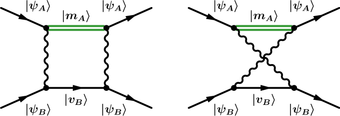
Figure 1: Ladder and crossed-ladder Feynman diagrams for the long-range interaction of atoms. The virtual state of atom $A$, labeled $|m_{A}\rangle$, is assumed to have a lower energy than the reference state.

From a QED point of view, the real part of the energy shift corresponding to the pole term is due to a very peculiar process, namely, resonant virtual emission into vacuum modes whose angular frequency matches the resonance condition $\omega=-E_{m,A}=|E_{m,A}|$. The resonant emission is accompanied by resonant absorption, and therefore leads to a real rather than imaginary energy shift. In the ladder and crossed-ladder Feynman diagrams (see Fig. 1), the virtual electron line of atom $A$, in state $|\psi_{A}\rangle$, would turn into a resonant lower-lying virtual state, whereas the ground-state atom line is excited into a “normal” energetically higher virtual state $|v_{B}\rangle$. The imaginary part of the pole term describes a process where the virtual photon becomes real and is emitted by the atom, in analogy to the imaginary part of the self energy Bethe (1947); Barbieri and Sucher (1978). Feynman propagators allow us to reduce the calculation to only two Feynman diagrams, which capture all possible time orderings (in contrast to time-ordered perturbation theory).

In Ref. Donaire et al. (2015), a situation of two non-identical atoms is considered, with mutually close resonance energies $\hbar\omega_{A}$ and $\hbar\omega_{B}$. Setting $E_{m,A}=-\hbar\omega_{A}$ and $E_{q,B}=\hbar\omega_{B}$, the authors of Ref. Donaire et al. (2015) assume that $\omega_{A}\approx\omega_{B}$, and define $\Delta_{AB}=\hbar\omega_{A}-\hbar\omega_{B}$ with $|\Delta_{AB}|\ll\hbar\omega_{A},\hbar\omega_{B}$. Furthermore, they restrict the sum over virtual states in Eq. (5) to the resonant state only, and they only keep the term $1/(E_{m,A}+E_{q,B})$ in the sum over virtual states, in the polarizability $\alpha_{B}(E_{m,A}/\hbar)$ [see Eq. (5)]. Under their assumptions [see Eq. (4) of Ref. Donaire et al. (2015)], $\left|1/(E_{m,A}+E_{q,B})\right|=\left|-1/\Delta_{AB}\right|\gg\left|1/(E_{q,B}-E_{m,A})\right|\approx 1/(2\hbar\omega_{B})$.

Under the restriction to the resonant virtual states, the direct term in Eq. (5) [proportional to $\alpha_{B,j\ell}\left(E_{m,A}/\hbar\right)$] matches that reported in Ref. Donaire et al. (2015) if we average the latter over the interaction time $T>2R/c$. Our result adds the contribution from nonresonant virtual states, which allow us to match the result with the close-range (van der Waals) limit, as well as the mixing term [proportional to $\alpha_{A\underline{B},j\ell}\left(E_{m,A}/\hbar\right)$] and the imaginary part of the energy shift (width term). For the mixing term to be nonzero, we need the orbital angular momentum quantum numbers to fulfill the relation $\ell_{A}=\ell_{B}$ or $\left|\ell_{A}-\ell_{B}\right|=2$, by virtue of the usual selection rules of atomic physics. Furthermore, we find that the full consideration of the Wick-rotated term and the pole term is crucial for obtaining numerically correct results for the interaction energies, for surprisingly large interatomic distances.

Numerical Calculations.—In the following, we aim to apply the developed formalism to $nD$–$1S$ atomic hydrogen systems. The interaction energy depends both on the spin orientation of the electron (total angular momentum $J$) as well as its projection $\mu$ onto the quantization axis Jentschura et al. (2017b). One may eliminate this dependence by evaluating the average over the fine-structure resolved states.

Short Range.—For interatomic separations in the range $a_{0}\ll R\ll a_{0}/\alpha$ (where $a_{0}$ is the Bohr radius), the interaction energy (2) is well approximated as $\Delta E\approx\Delta E_{\rm vdW}$ where

$$\Delta E_{\rm vdW}= \;-\frac{1}{(4\pi\epsilon_{0})^{2}}\frac{\beta_{ij}\,\beta_{k\ell}}{R^{6}}\,\sum_{v}\sum_{q}\frac{1}{E_{v,A}+E_{q,B}}$$

$$\;\times\left[\left<\psi_{A}\left|d_{Ai}\right|v_{A}\right>\left<v_{A}\left|d_{Ak}\right|\psi_{A}\right>\right.$$

$$\hskip 50.0pt\times\left<\psi_{B}\left|d_{Bj}\right|q_{B}\right>\left<q_{B}\left|d_{B\ell}\right|\psi_{B}\right>$$

$$\pm\left<\psi_{A}\left|d_{Ai}\right|v_{A}\right>\left<v_{B}\left|d_{Bk}\right|\psi_{B}\right>$$

$$\left.\hskip 50.0pt\times\left<\psi_{B}\left|d_{Bj}\right|q_{B}\right>\left<q_{A}\left|d_{A\ell}\right|\psi_{A}\right>\right]\,,$$

$$= \;-\frac{1}{R^{6}}\left(D_{6}\left(A;B\right)\pm M_{6}\left(A;B\right)\right)\,.$$ (8)

Here, $D_{6}$ is the direct, and $M_{6}$ is the mixing van der Waals coefficient Chibisov (1972); Deal and Young (1973); Adhikari et al. (2017); Jentschura et al. (2017a); Power and Thirunamachandran (1995); Safari et al. (2006). For energetically lower states in atom $A$ (with $E_{v,A}=E_{m,A}<0$), the representation (Virtual Resonant Emission and Oscillatory Long–Range Tails in van der Waals Interactions of Excited States: QED Treatment and Applications) is obtained by carefully considering the contributions from the Wick-rotated term ${\mathcal{W}}$ and the pole term ${\mathcal{P}}$.

For the fine-structure average of the direct term $D_{6}$, we have

$$\langle D_{6}(nD;1S)\rangle=\langle D_{6}^{\left(P\right)}(nD;1S)\rangle+\langle D_{6}^{\left(F\right)}(nD;1S)\rangle\,,$$ (9)

where the virtual-$P$-state contribution $\langle D_{6}^{\left(P\right)}(nD;1S)\rangle$ and the virtual-$F$-state contribution $\langle D_{6}^{\left(F\right)}(nD;1S)\rangle$ are given in Table 1. Numerically, we find that the mixing term $M_{6}$ is smaller than the direct term $D_{6}$, by at least four orders of magnitude, for all fine-structure resolved $nD$ states, for all distance ranges investigated in this Letter. This trend follows the pattern observed for the van der Waals coefficients (Table 1) and is in contrast to the $2S$–$1S$ system, where both terms are of comparable magnitude Chibisov (1972); Adhikari et al. (2017).

Table 1: Van der Waals $D_{6}$ (direct) coefficients, for $nD$–$1S$ interactions, averaged over the total angular momenta and magnetic projections of the excited $D$ state. The coefficients are given in units of $E_{h}\,a_{0}^{6}$.

Coefficient	Virtual $P$	Virtual $F$	Total
$\langle D_{6}(8D;1S)\rangle$	17459.439	26156.866	43616.296
$\langle D_{6}(10D;1S)\rangle$	43476.563	65182.580	108659.144
$\langle D_{6}(12D;1S)\rangle$	91115.328	136640.733	227756.061

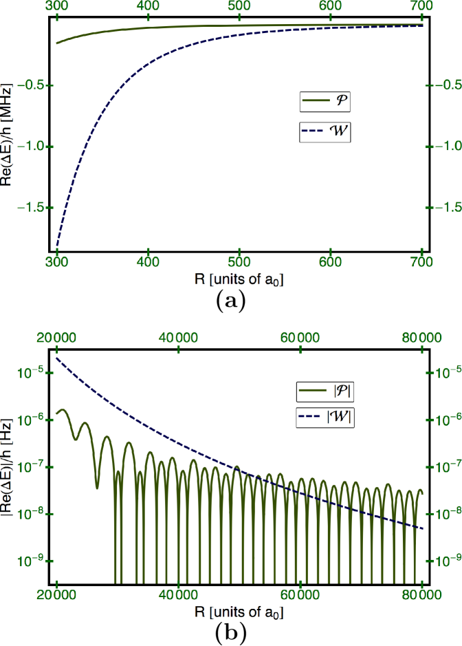
Figure 2: The upper panel (a) compares the Wick-rotated term ${\mathcal{W}}$ (dashed line) to the real part ${\mathcal{P}}={\rm Re}\,{\mathcal{Q}}$ of the pole term (solid line) for the $12D$–$1S$ interaction (fine-structure average) in the intermediate range $a_{0}/\alpha\lesssim R\ll\hbar c/{\mathcal{L}}$. The interaction energy is $\Delta E={\mathcal{Q}}+{\mathcal{W}}$. The Wick-rotated term dominates despite parametric suppression [see Eq. (10)]. The lower panel (b) displays the logarithm of the modulus of the interaction energy (Wick-rotated term versus pole term) for very large interatomic distance; the pole term finally dominates. The oscillations of the pole term are dominated by virtual $2P$ state contribution; when the interaction energy changes sign, the logarithm diverges to $-\infty$.

Long Range.—One might think that the $1/R^{2}$ pole term from Eq. (5) should easily dominate the interaction energy in the range $R\gg a_{0}/\alpha$. Indeed, power counting in the fine-structure constant $\alpha$, according to Ref. Bethe and Salpeter (1957), shows that the cosine and sine terms in ${\mathcal{P}}$ are asymptotically given by

$$\frac{{\mathcal{P}}_{\rm cos}}{E_{h}}\sim \;\left\{\frac{\alpha^{4}}{\rho^{2}}\cos(\alpha\,\rho)\,,\frac{\alpha^{2}}{\rho^{4}}\cos(\alpha\,\rho)\,,\frac{1}{\rho^{6}}\cos(\alpha\,\rho)\right\}\,,$$ (10a)

$$\frac{{\mathcal{P}}_{\rm sin}}{E_{h}}\sim \;\left\{\frac{\alpha^{3}}{\rho^{3}}\sin(\alpha\,\rho)\,,\frac{\alpha}{\rho^{5}}\sin(\alpha\,\rho)\right\}\,,$$ (10b)

where $$\rho=R/a_{0} E_{h}$$ and is the Hartree energy. A comparison to the van der Waals term, given in Eq. (Virtual Resonant Emission and Oscillatory Long–Range Tails in van der Waals Interactions of Excited States: QED Treatment and Applications), and the Wick-rotated term (4),

$$\Delta E_{\rm vdW}\sim\frac{E_{h}}{\rho^{6}}\,,\qquad{\mathcal{W}}\;\mathop{\sim}^{\rho\gg 1/\alpha}\;\frac{E_{h}}{\alpha\,\rho^{7}}\,,$$ (10c)

shows that all terms (pole term, Wick-rotated, and van der Waals) are of the same order-of-magnitude for $\rho\sim 1/\alpha$, while the pole term should parametrically dominate for $\rho>1/\alpha$. However, this consideration does not take into account the scaling of the terms with the principal quantum number $n$. While we find that the $D_{6}$ coefficients typically grow as $n^{4}$ for a given manifold of states (see also Ref. C. M. Adhikari et al. (2017)), the energy differences $E_{m,A}$ for adjacent lower-lying states are proportional to $1/(n-1)^{2}-1/n^{2}\sim 1/n^{3}$ for large $n$, and the fourth power of the energy difference $E_{m,A}$ enters the prefactor of the $1/R^{2}$ pole term. Hence, it is interesting to compare the parametric estimates to a concrete calculation for excited $nD$ states; this is also important in order to gauge the importance of the nonresonant contributions to the interaction energy which were left out in Ref. Donaire et al. (2015).

But let us first write down the leading asymptotic terms, for all long-range contributions of interest. For $R\gg\hbar c/{\mathcal{L}}$, where ${\mathcal{L}}$ is the Lamb shift energy of about $1\,{\rm GHz}$ (see Ref. Adhikari et al. (2017)), the Wick-rotated contribution attains the familiar $1/R^{7}$ asymptotics from the Casimir–Polder formalism Casimir and Polder (1948),

$${\mathcal{W}}^{\left(\mathrm{dir}\right)}\mathop{=}^{R\to\infty}-\frac{\hbar c}{8\pi}\frac{\alpha_{nD,ij}(0)\alpha_{1S}(0)}{(4\pi\epsilon_{0})^{2}\,R^{7}}\left(13\,\delta_{ij}+15\frac{R_{i}R_{j}}{R^{2}}\right)\,.$$ (11)

This tail is parametrically suppressed in comparison to the leading $1/R^{2}$ pole contribution,

$${\mathcal{P}}^{\left(\mathrm{dir}\right)}\mathop{=}^{R\to\infty}-\sum_{E_{m}<E_{nD}}\left(\frac{E_{m,A}}{\hbar c}\right)^{4}\,\frac{\cos\left(2\frac{E_{m,A}}{\hbar c}R\right)}{(4\pi\epsilon_{0})^{2}\,R^{2}}\,\\[0.05728pt] \times\alpha_{ij}\left<nD\left|d_{Ai}\right|m_{A}\right>\left<m_{A}\left|d_{Aj}\right|nD\right>\,\alpha_{1S}\left(\frac{E_{m,A}}{\hbar}\right)\,.$$ (12)

In the intermediate range $a_{0}\ll R\ll\hbar c/{\mathcal{L}}$, the Wick-rotated contribution has a nonretarded $1/R^{6}$ tail, due to a nonretarded contribution from virtual $nP$ and $nF$ states which are displaced from the $nD$ state only by the Lamb shift [see Eqs. (23) and (24) of Ref. Adhikari et al. (2017)],

$${\mathcal{W}}^{\left(\mathrm{dir}\right)}\sim-\frac{\overline{D}_{6}(nD;1S)}{R^{6}}\,,\qquad\frac{a_{0}}{\alpha}\ll R\ll\frac{\hbar c}{{\mathcal{L}}}\,.$$ (13)

The fine-structure average of $\overline{D}_{6}(nD;1S)$ is given by Jentschura et al. (2017b)

$$\langle\overline{D}_{6}(nD;1S)\rangle=\frac{81}{8}n^{2}\,(n^{2}-7)\,.$$ (14)

For the mixing term, simplifications are scarce; the leading long-range asymptotics of the Wick-rotated term read

$${\mathcal{W}}^{\left(\mathrm{mix}\right)}\mathop{=}^{R\to\infty}\;-\frac{\hbar c}{8\pi}\frac{\alpha_{\underline{nD}\,1S,ik}(0)\,\alpha_{nD\,\underline{1S},j\ell}(0)}{(4\pi\epsilon_{0})^{2}\,R^{7}}\\ \times\left(3\alpha_{ij}\alpha_{kl}+5\alpha_{ij}\beta_{kl}+5\beta_{ij}\beta_{kl}\right)\,.$$ (15)

The leading pole contribution (in the long range) is given by a sum over virtual $P$ states which enter the mixed polarizability $\alpha_{nD\,\underline{1S},j\ell}$,

$${\mathcal{P}}^{\left(\mathrm{mix}\right)}\mathop{=}^{R\to\infty}-\frac{\sum_{E_{m}<E_{nD}}}{(4\pi\epsilon_{0})^{2}}\left(\frac{E_{m,A}}{\hbar c}\right)^{4}\frac{\cos\left(2\frac{E_{m,A}}{\hbar c}R\right)}{R^{2}}\\[0.05728pt] \times\alpha_{ij}\,\alpha_{kl}\,\alpha_{nD\,\underline{1S},j\ell}\left(\frac{E_{m,A}}{\hbar}\right)\\[0.4878pt] \times\,\left<nD\left|d_{Ai}\right|m_{A}\right>\left<m_{A}\left|d_{Ak}\right|1S\right>\,.$$ (16)

In the intermediate range, one has

$${\mathcal{W}}^{\left(\mathrm{mix}\right)}\sim-\frac{\overline{M}_{6}(nD;1S)}{R^{6}}\,,\qquad\frac{a_{0}}{\alpha}\ll R\ll\frac{\hbar c}{{\mathcal{L}}}\,,$$ (17)

where $\overline{M}_{6}(nD;1S)$ is the generalization of $\overline{D}_{6}$ to the mixing term [see Ref. Jentschura et al. (2017b) and Eq. (67) of Ref. Adhikari et al. (2017)].

In Fig. 2, we compare the magnitude of the Wick-rotated term and the pole term in the intermediate range $a_{0}/\alpha\ll R\ll\hbar c/{\mathcal{L}}$, and for very large separations $R\sim\hbar c/{\mathcal{L}}$. While a parametric analysis [Eq. (10)] would suggest dominance of the pole term in the intermediate range, a numerical calculation reveals a different behavior, with the Wick-rotated term dominating the interaction, due to the variability of the numerical coefficients multiplying the parametric estimates given in Eq. (10).

Conclusions.—We have shown that the consistent use of Feynman propagators and the concomitant virtual photon integration contours lead to the prediction of long-range tails for excited-state van der Waals interactions. Pole terms are picked up for virtual states $\left|v_{A}\right>=\left|m_{A}\right>$ of lower energy than the reference state of the excited atom $A$. The pole contribution ${\mathcal{Q}}$ to the energy shift is complex rather than real (includes a width term $\Gamma=-2\,{\rm Im}{\mathcal{Q}}$), is spacewise-oscillating and in the long-range, behaves as $\cos[2(E_{m}-E_{A})\,R/(\hbar c)]/R^{2}$, where $E_{A}$ is the reference state energy and $E_{m}<E_{A}$ that of the low-energy virtual state. For excited states, both the direct as well as the exchange (gerade-ungerade mixing) term can be expressed as a sum of a Wick-rotated contribution [Eq. (4)], and a pole term [Eq. (5)]. Our inclusion of the nonresonant terms in the interaction energy enables us to match the very-long-range, oscillatory result against the well-known close-range, nonretarded van der Waals limit, and to carry out numerical calculations in the intermediate region. We also include the width term, and the gerade-ungerade mixing term which pertains to excited-state interactions of identical atoms.

For $nD$–$1S$ interactions, we have shown that despite parametric suppression, the Wick-rotated term, which is non-oscillatory and contains the non-resonant states, still dominates in the intermediate distance range $a_{0}/\alpha\lesssim R\ll\hbar c/{\mathcal{L}}$ (see Fig. 2). The very-long-range, oscillatory tail of the van der Waals interaction is relevant only for very large interatomic distances. This conclusion holds for $nD$–$1S$ interactions as well as $nS$–$1S$ systems Jentschura et al. (2017b); C. M. Adhikari et al. (2017). The reason for the suppression is that the numerical coefficients which multiply the parametric estimates given in Eq. (10) drastically depend on the particular term in the van der Waals energy. This is in part due to the scaling of the coefficients with the principal quantum number. E.g., for $nD$–$1S$ interactions, the $1/R^{2}$ leading oscillatory tail from Eq. (5) is of order $E_{h}\,\alpha^{4}\,\cos(\alpha\,\rho)/\rho^{2}$, yet multiplied by numerical coefficients of order $10^{-6}$ [in addition to the factor $\alpha^{4}$; see the supplementary material Jentschura et al. (2017b), Eq. (14), Table 1 and Fig. 2]. By contrast, the non-oscillatory terms of order $E_{h}/\rho^{6}$ are multiplied by coefficients of order $10^{4}\ldots 10^{6}$. This behavior of the coefficients changes any predictions based on the parametric estimates given in Eq. (10) by ten orders of magnitude as compared to a situation with coefficients of order unity.

Our results are important for an improved analysis of pressure shifts, and fluctuating-dipole-induced energy shift, for atomic beam spectroscopy with Rydberg states, where these effects have been identified as notoriously problematic in recent years (see pp. 134 and 151 of Ref. deVries ). An improved determination of the Rydberg constant based on Rydberg-state spectroscopy could resolve the muonic hydrogen proton radius puzzle, because the smaller proton radius measured in Ref. R. Pohl et al. [CREMA Collaboration] (2010, 2016) leads to a Rydberg constant which is discrepant with regard to the current CODATA value R. Pohl et al. [CREMA Collaboration] (2010); Mohr et al. (2016).

Acknowledgments.—This research has been supported by the NSF (grant PHY–1403937).

References

- Casimir and Polder (1948) H. B. G. Casimir and D. Polder, “The Influence of Radiation on the London-van-der-Waals Forces,” Phys. Rev. 73, 360–372 (1948).
- Chibisov (1972) M. I. Chibisov, “Dispersion Interaction of Neutral Atoms,” Opt. Spectrosc. 32, 1–3 (1972).
- Deal and Young (1973) W. J. Deal and R. H. Young, “Long–Range Dispersion Interactions Involving Excited Atoms; the H(1s)—H(2s) Interaction,” Int. J. Quantum Chem. 7, 877–892 (1973).
- Adhikari et al. (2017) C. M. Adhikari, V. Debierre, A. Matveev, N. Kolachevsky, and U. D. Jentschura, “Long-range interactions of hydrogen atoms in excited states. I. – interactions and Dirac– perturbations,” Phys. Rev. A 95, 022703 (2017).
- Jentschura et al. (2017a) U. D. Jentschura, V. Debierre, C. M. Adhikari, A. Matveev, and N. Kolachevsky, “Long-range interactions of excited hydrogen atoms. II. Hyperfine-resolved – system,” Phys. Rev. A 95, 022704 (2017a).
- Power and Thirunamachandran (1995) E. A. Power and T. Thirunamachandran, “Dispersion forces between molecules with one or both molecules excited,” Phys. Rev. A 51, 3660–3666 (1995).
- Safari et al. (2006) H. Safari, S. Y. Buhmann, D.-G. Welsch, and H. T. Dung, “Body-assisted van der Waals interaction between two atoms,” Phys. Rev. A 74, 042101 (2006).
- Safari and Karimpour (2015) H. Safari and M. R. Karimpour, “Body-Assisted van der Waals Interaction between Excited Atoms,” Phys. Rev. Lett. 114, 013201 (2015).
- Berman (2015) P. R. Berman, “Interaction energy of nonidentical atoms,” Phys. Rev. A 91, 042127 (2015).
- Milonni and Rafsanjani (2015) P. W. Milonni and S. M. H. Rafsanjani, “Distance dependence of two-atom dipole interactions with one atom in an excited state,” Phys. Rev. A 92, 062711 (2015).
- Donaire et al. (2015) M. Donaire, R. Guérout, and A. Lambrecht, “Quasiresonant van der Waals Interaction between Nonidentical Atoms,” Phys. Rev. Lett. 115, 033201 (2015).
- Donaire (2016) M. Donaire, “Two-atom interaction energies with one atom in an excited state: van der Waals potentials versus level shifts,” Phys. Rev. A 93, 052706 (2016).
- Gomberoff et al. (1966) L. Gomberoff, R. R. McLone, and E. A. Power, “Long–Range Retarded Potentials between Molecules,” J. Chem. Phys. 44, 4148–4153 (1966).
- Biraben et al. (1989) F. Biraben, J.-C. Garreau, L. Julien, and M. Allegrini, “New Measurement of the Rydberg Constant by Two-Photon Spectroscopy of Hydrogen Rydberg States,” Phys. Rev. Lett. 62, 621–621 (1989).
- de Beauvoir et al. (1997) B. de Beauvoir, F. Nez, L. Julien, B. Cagnac, F. Biraben, D. Touahri, L. Hilico, O. Acef, A. Clairon, and J. J. Zondy, “Absolute Frequency Measurement of the – Transitions in Hydrogen and Deuterium: New Determination of the Rydberg Constant,” Phys. Rev. Lett. 78, 440–443 (1997).
- Schwob et al. (1999) C. Schwob, L. Jozefowski, B. de Beauvoir, L. Hilico, F. Nez, L. Julien, F. Biraben, O. Acef, J. J. Zondy, and A. Clairon, “Optical Frequency Measurement of the - Transitions in Hydrogen and Deuterium: Rydberg Constant and Lamb Shift Determinations,” Phys. Rev. Lett. 82, 4960–4963 (1999), [Erratum Phys. Rev. 86, 4193 (2001)].
- (17) J. C. deVries, Ph.D. thesis, Massachusetts Institute of Technology, Cambridge, MA (2002), URL https://dspace.mit.edu/handle/1721.1/4108.
- Berestetskii et al. (1982) V. B. Berestetskii, E. M. Lifshitz, and L. P. Pitaevskii, Quantum Electrodynamics, Volume 4 of the Course on Theoretical Physics, 2nd ed. (Pergamon Press, Oxford, UK, 1982).
- Jentschura et al. (2017b) U. D. Jentschura, C. M. Adhikari, and V. Debierre, Long–Range Tails in van der Waals Interactions of Excited–State Atoms: Mixing Terms, Notes and Derivations [Supplementary Material for Physical Review Letters] (2017b).
- Bethe (1947) H. A. Bethe, “The Electromagnetic Shift of Energy Levels,” Phys. Rev. 72, 339–341 (1947).
- Barbieri and Sucher (1978) R. Barbieri and J. Sucher, “General Theory of Radiative Corrections to Atomic Decay Rates,” Nucl. Phys. B 134, 155–168 (1978).
- Bethe and Salpeter (1957) H. A. Bethe and E. E. Salpeter, Quantum Mechanics of One- and Two-Electron Atoms (Springer, Berlin, 1957).
- C. M. Adhikari et al. (2017) C. M. Adhikari et al., Long-range interactions of hydrogen atoms in excited states. III. – interactions for , in preparation (2017).
- R. Pohl et al. [CREMA Collaboration] (2010) R. Pohl et al. [CREMA Collaboration], “The size of the proton,” Nature (London) 466, 213–216 (2010).
- R. Pohl et al. [CREMA Collaboration] (2016) R. Pohl et al. [CREMA Collaboration], “Laser spectroscopy of muonic deuterium,” Science 353, 669–673 (2016).
- Mohr et al. (2016) P. J. Mohr, D. B. Newell, and B. N. Taylor, “CODATA Recommended Values of the Fundamental Physical Constants: 2014,” Rev. Mod. Phys. 88, 035009 (2016).