[-1cm]-3cm

University of Liège
Faculty of Applied Sciences

Department of Electrical Engineering & Computer Science

Montefiore Institute

PhD Thesis in Engineering Sciences

EXPLOITING RANDOM PROJECTIONS AND SPARSITY WITH RANDOM FORESTS AND GRADIENT BOOSTING METHODS

Application to multi-label and multi-output learning, random forest model compression and leveraging input sparsity

arnaud joly

advisor: louis wehenkel

co-advisor: pierre geurts

December 2016

Copyright.1Copyright.1CopyrightCopyrightCopyright.1

Jury members.1Jury members.1Jury membersJury membersJury members.1

Jury members

Damien Ernst, Professor at the Université de Liège (President);

Louis Wehenkel, Professor at the Université de Liège (Advisor);

Pierre Geurts, Professor at the Université de Liège (Co-Advisor);

Quentin Louveaux, Professor at Université de Liège;

Ashwin Ittoo, Professor at the Université de Liège;

Grigorios Tsoumakas, Professor at the Aristotle University of Thessaloniki;

Celine Vens, Professor at the Katholieke Universiteit Leuven;

Abstract.1Abstract.1AbstractAbstractAbstract.1

Abstract

Within machine learning, the supervised learning field aims at modeling the input-output relationship of a system, from past observations of its behavior. Decision trees characterize the input-output relationship through a series of nested $if-then-else$ questions, the testing nodes, leading to a set of predictions, the leaf nodes. Several of such trees are often combined together for state-of-the-art performance: random forest ensembles average the predictions of randomized decision trees trained independently in parallel, while tree boosting ensembles train decision trees sequentially to refine the predictions made by the previous ones.

The emergence of new applications requires scalable supervised learning algorithms in terms of computational power and memory space with respect to the number of inputs, outputs, and observations without sacrificing accuracy. In this thesis, we identify three main areas where decision tree methods could be improved for which we provide and evaluate original algorithmic solutions: (i) learning over high dimensional output spaces, (ii) learning with large sample datasets and stringent memory constraints at prediction time and (iii) learning over high dimensional sparse input spaces.

A first approach to solve learning tasks with a high dimensional output space, called binary relevance or single target, is to train one decision tree ensemble per output. However, it completely neglects the potential correlations existing between the outputs. An alternative approach called multi-output decision trees fits a single decision tree ensemble targeting simultaneously all the outputs, assuming that all outputs are correlated. Nevertheless, both approaches have (i) exactly the same computational complexity and (ii) target extreme output correlation structures. In our first contribution, we show how to combine random projection of the output space, a dimensionality reduction method, with the random forest algorithm decreasing the learning time complexity. The accuracy is preserved, and may even be improved by reaching a different bias-variance tradeoff. In our second contribution, we first formally adapt the gradient boosting ensemble method to multi-output supervised learning tasks such as multi-output regression and multi-label classification. We then propose to combine single random projections of the output space with gradient boosting on such tasks to adapt automatically to the output correlation structure.

The random forest algorithm often generates large ensembles of complex models thanks to the availability of a large number of observations. However, the space complexity of such models, proportional to their total number of nodes, is often prohibitive, and therefore these modes are not well suited under stringent memory constraints at prediction time. In our third contribution, we propose to compress these ensembles by solving a $\ell_{1}$-based regularization problem over the set of indicator functions defined by all their nodes.

Some supervised learning tasks have a high dimensional but sparse input space, where each observation has only a few of the input variables that have non zero values. Standard decision tree implementations are not well adapted to treat sparse input spaces, unlike other supervised learning techniques such as support vector machines or linear models. In our fourth contribution, we show how to exploit algorithmically the input space sparsity within decision tree methods. Our implementation yields a significant speed up both on synthetic and real datasets, while leading to exactly the same model. It also reduces the required memory to grow such models by exploiting sparse instead of dense memory storage for the input matrix.

Résumé.1Résumé.1RésuméRésuméRésumé.1

Résumé

Parmi les techniques d’apprentissage automatique, l’apprentissage supervisé vise à modéliser les relations entrée-sortie d’un système, à partir d’observations de son fonctionnement. Les arbres de décision caractérisent cette relation entrée-sortie à partir d’un ensemble hiérarchique de questions appelées les noeuds tests amenant à une prédiction, les noeuds feuilles. Plusieurs de ces arbres sont souvent combinés ensemble afin d’atteindre les performances de l’état de l’art: les ensembles de forêts aléatoires calculent la moyenne des prédictions d’arbres de décision randomisés, entraînés indépendamment et en parallèle alors que les ensembles d’arbres de boosting entraînent des arbres de décision séquentiellement, améliorant ainsi les prédictions faites par les précédents modèles de l’ensemble.

L’apparition de nouvelles applications requiert des algorithmes d’apprentissage supervisé efficaces en terme de puissance de calcul et d’espace mémoire par rapport au nombre d’entrées, de sorties, et d’observations sans sacrifier la précision du modèle. Dans cette thèse, nous avons identifié trois domaines principaux où les méthodes d’arbres de décision peuvent être améliorées pour lequel nous fournissons et évaluons des solutions algorithmiques originales: (i) apprentissage sur des espaces de sortie de haute dimension, (ii) apprentissage avec de grands ensembles d’échantillons et des contraintes mémoires strictes au moment de la prédiction et (iii) apprentissage sur des espaces d’entrée creux de haute dimension.

Une première approche pour résoudre des tâches d’apprentissage avec un espace de sortie de haute dimension, appelée «binary relevance» ou «single target», est l’apprentissage d’un ensemble d’arbres de décision par sortie. Toutefois, cette approche néglige complètement les corrélations potentiellement existantes entre les sorties. Une approche alternative, appelée «arbre de décision multi-sorties», est l’apprentissage d’un seul ensemble d’arbres de décision pour toutes les sorties, faisant l’hypothèse que toutes les sorties sont corrélées. Cependant, les deux approches ont (i) exactement la même complexité en temps de calcul et (ii) visent des structures de corrélation de sorties extrêmes. Dans notre première contribution, nous montrons comment combiner des projections aléatoires (une méthode de réduction de dimensionnalité) de l’espace de sortie avec l’algorithme des forêts aléatoires diminuant la complexité en temps de calcul de la phase d’apprentissage. La précision est préservée, et peut même être améliorée en atteignant un compromis biais-variance différent. Dans notre seconde contribution, nous adaptons d’abord formellement la méthode d’ensemble «gradient boosting» à la régression multi-sorties et à la classification multi-labels. Nous proposons ensuite de combiner une seule projection aléatoire de l’espace de sortie avec l’algorithme de «gradient boosting» sur de telles tâches afin de s’adapter automatiquement à la structure des corrélations existant entre les sorties.

Les algorithmes de forêts aléatoires génèrent souvent de grands ensembles de modèles complexes grâce à la disponibilité d’un grand nombre d’observations. Toutefois, la complexité mémoire, proportionnelle au nombre total de noeuds, de tels modèles est souvent prohibitive, et donc ces modèles ne sont pas adaptés à des contraintes mémoires fortes lors de la phase de prédiction. Dans notre troisième contribution, nous proposons de compresser ces ensembles en résolvant un problème de régularisation basé sur la norme $\ell_{1}$ sur l’ensemble des fonctions indicatrices défini par tous leurs noeuds.

Certaines tâches d’apprentissage supervisé ont un espace d’entrée de haute dimension mais creux, où chaque observation possède seulement quelques variables d’entrée avec une valeur non-nulle. Les implémentations standards des arbres de décision ne sont pas adaptées pour traiter des espaces d’entrée creux, contrairement à d’autres techniques d’apprentissage supervisé telles que les machines à vecteurs de support ou les modèles linéaires. Dans notre quatrième contribution, nous montrons comment exploiter algorithmiquement le creux de l’espace d’entrée avec les méthodes d’arbres de décision. Notre implémentation diminue significativement le temps de calcul sur des ensembles de données synthétiques et réelles, tout en fournissant exactement le même modèle. Cela permet aussi de réduire la mémoire nécessaire pour apprendre de tels modèles en exploitant des méthodes de stockage appropriées pour la matrice des entrées.

acknowledgments.1acknowledgments.1AcknowledgmentsAcknowledgmentsacknowledgments.1

Introduction

Progress in information technology enables the acquisition and storage of growing amounts of rich data in many domains including science (biology, high-energy physics, astronomy, etc.), engineering (energy, transportation, production processes, etc.), and society (environment, commerce, etc.). Connected objects, such as smartphones, connected sensors or intelligent houses, are now able to record videos, images, audio signals, object localizations, temperatures, social interactions of the user through a social network, phone calls or user to computer program interactions such as voice help assistant or web search queries. The accumulating datasets come in various forms such as images, videos, time-series of measurements, recorded transactions, text etc. WEB technology often allows one to share locally acquired datasets, and numerical simulation often allows one to generate low cost datasets on demand. Opportunities exist thus for combining datasets from different sources to search for generic knowledge and enable robust decision.

All these rich datasets are of little use without the availability of automatic procedures able to extract relevant information from them in a principled way. In this context, the field of machine learning aims at developing theory and algorithmic solutions for the extraction of synthetic patterns of information from all kinds of datasets, so as to help us to better understand the underlying systems generating these data and hence to take better decisions for their control or exploitation.

Among the machine learning tasks, supervised learning aims at modeling a system by observing its behavior through samples of pairs of inputs and outputs. The objective of the generated model is to predict with high accuracy the outputs of the system given previously unseen inputs. A genomic application of supervised learning would be to model how a DNA sequence, a biological code, is linked to some genetic diseases. The samples used to fit the model are the input-output pairs obtained by sequencing the genome, the inputs, of patients with known medical records for the studied genetic diseases, the outputs. The objective is here twofold: (i) to understand how the DNA sequence influences the appearing of the studied genetic diseases and (ii) to use the predictive models to infer the probability of contracting the genetic disease.

The emergence of new applications, such as image annotation, personalized advertising or 3D image segmentation, leads to high dimensional data with a large number of inputs and outputs. It requires scalable supervised learning algorithms in terms of computational power and memory space without sacrificing accuracy.

Decision trees Breiman et al. (1984) are supervised learning models organized in the form of a hierarchical set of questions each one typically based on one input variable leading to a prediction. Used in isolation, trees are generally not competitive in terms of accuracy, but when combined into ensembles Breiman (2001); Friedman (2001), they yield state-of-the-art performances on standard benchmarks Caruana et al. (2008); Fernández-Delgado et al. (2014); Madjarov et al. (2012). They however suffer from several limitations that make them not always suited to address modern applications of machine learning techniques in particular involving high dimensional input and output spaces.

In this thesis, we identify three main areas where random forest methods could be improved and for which we provide and evaluate original algorithmic solutions: (i) learning over high dimensional output spaces, (ii) learning with large sample datasets and stringent memory constraints at prediction time and (iii) learning over high dimensional sparse input spaces. We discuss each one of these solutions in the following paragraphs.

High dimensional output spaces

New applications of machine learning have multiple output variables, potentially in very high number Agrawal et al. (2013); Dekel and Shamir (2010), associated to the same set of input variables. A first approach to address such multi-output tasks is the so-called binary relevance / single target method Tsoumakas et al. (2009); Spyromitros-Xioufis et al. (2016), which separately fits one decision tree ensemble for each output variable, assuming that the different output variables are independent. A second approach called multi-output decision trees Blockeel et al. (2000); Geurts et al. (2006b); Kocev et al. (2013) fits a single decision tree ensemble targeting simultaneously all the outputs, assuming that all outputs are correlated. However in practice, (i) the computational complexity is the same for both approaches and (ii) we have often neither of these two extreme output correlation structures. As our first contribution, we show how to make random forest faster by exploiting random projections (a dimensionality reduction technique) of the output space. As a second contribution, we show how to combine gradient boosting of tree ensembles with single random projections of the output space to automatically adapt to a wide variety of correlation structures.

Memory constraints on model size

Even with a large number of training samples $n$, random forest ensembles have good computational complexity ($O(n\log{n})$) and are easily parallelizable leading to the generation of very large ensembles. However, the resulting models are big as the model complexity is proportional to the number of samples $n$ and the ensemble size. As our third contribution, we propose to compress these tree ensembles by solving an appropriate optimization problem.

High dimensional sparse input spaces

Some supervised learning tasks have very high dimensional input spaces, but only a few variables have non zero values for each sample. The input space is said to be “sparse”. Instances of such tasks can be found in text-based supervised learning, where each sample is often mapped to a vector of variables corresponding to the (frequency of) occurrence of all words (or multigrams) present in the dataset. The problem is sparse as the size of the text is small compared to the number of possible words (or multigrams). Standard decision tree implementations are not well adapted to treat sparse input spaces, unlike models such as support vector machines Cortes and Vapnik (1995); Scholkopf and Smola (2001) or linear models Bottou (2012). Decision tree implementations are indeed treating these sparse variables as dense ones raising the memory needed. The computational complexity also does not depend upon the fraction of non zero values. As a fourth contribution, we propose an efficient decision tree implementation to treat supervised learning tasks with sparse input spaces.

1   Publications

This dissertation features several publications about random forest algorithms:

• Joly et al. (2014) A. Joly, P. Geurts, and L. Wehenkel. Random forests with random projections of the output space for high dimensional multi-label classification. In Machine Learning and Knowledge Discovery in Databases, pages 607–622. Springer Berlin Heidelberg, 2014.

• Joly et al. (2012) A. Joly, F. Schnitzler, P. Geurts, and L. Wehenkel. L1-based compression of random forest models. In European Symposium on Artificial Neural Networks, Computational Intelligence and Machine Learning, 2012.

• Buitinck et al. (2013) L. Buitinck, G. Louppe, M. Blondel, F. Pedregosa, A. Mueller, O. Grisel, V. Niculae, P. Prettenhofer, A. Gramfort, J. Grobler, R. Layton, J. Vanderplas, A. Joly, B. Holt, and G. Varoquaux. Api design for machine learning software: experiences from the scikit-learn project. arXiv preprint arXiv:1309.0238, 2013.

and also the following submitted article:

• H. Fares, A. Joly, and P. Papadimitriou. Scalable Learning of Tree-Based Models on Sparsely Representable Data.

Some collaborations were made during the thesis, but are not discussed within this manuscript:

• Sutera et al. (2014) A. Sutera, A. Joly, V. François-Lavet, Z. A. Qiu, G. Louppe, D. Ernst, and P. Geurts. Simple connectome inference from partial correlation statistics in calcium imaging. In JMLR: Workshop and Conference Proceedings, pages 1–12, 2014.

• Delierneux et al. (2015a) C. Delierneux, N. Layios, A. Hego, J. Huart, A. Joly, P. Geurts, P. Damas, C. Lecut, A. Gothot, and C. Oury. Elevated basal levels of circulating activated platelets predict icu-acquired sepsis and mortality: a prospective study. Critical Care, 19(Suppl 1):P29, 2015a.

• Delierneux et al. (2015b) C. Delierneux, N. Layios, A. Hego, J. Huart, A. Joly, P. Geurts, P. Damas, C. Lecut, A. Gothot, and C. Oury. Prospective analysis of platelet activation markers to predict severe infection and mortality in intensive care units. In journal of thrombosis and haemostasis, volume 13, pages 651–651.

• Begon et al. (2016) J.-M. Begon, A. Joly, and P. Geurts. Joint learning and pruning of decision forests. In Belgian-Dutch Conference On Machine Learning, 2016.

The following article has been submitted:

• C. Delierneux, N. Layios, A. Hego, J. Huart, C. Gosset, C. Lecut, N. Maes, P. Geurts, A. Joly, P. Lancellotti, P. Damas, A. Gothot, and C. Oury. Incremental value of platelet markers to clinical variables for sepsis prediction in intensive care unit patients: a prospective pilot study.

2   Outline

In Part i of this thesis, we start by introducing in Chapter 2 the key concepts about supervised learning: (i) what are the most popular supervised learning models, (ii) how to assess the prediction performance of a supervised learning model and (iii) how to optimize the hyper-parameters of theses models. We also present some unsupervised projection methods, such as random projections, which transform the original space to another one. We describe more in detail the decision tree model classes in Chapter 3. More specifically, we describe the methodology to grow and to prune such trees. We also show how to adapt decision tree growing and prediction algorithms to multi-output tasks. In Chapter 4, we show why and how to combine models into ensembles either by learning models independently with averaging methods or sequentially with boosting methods.

In Part ii, we first show how to grow an ensemble of decision trees on very high dimensional output spaces by projecting the original output space onto a random sub-space of lower dimension. In Chapter 5, it turns out that for random forest models, an averaging ensemble of decision trees, the learning time complexity can be reduced without affecting the prediction performance. Furthermore, it may lead to accuracy improvement Joly et al. (2014). In Chapter 6, we propose to combine random projections of the output space and the gradient tree boosting algorithm, while reducing learning time and automatically adapting to any output correlation structure.

In Part iii, we leverage sparsity in the context of decision tree ensembles. In Chapter 7, we exploit sparsifying optimization algorithms to compress random forest models while retaining their prediction performances Joly et al. (2012). In Chapter 8, we show how to leverage input sparsity to speed up decision tree induction.

During the thesis, I made significant contributions to the open source scikit-learn project Pedregosa et al. (2011); Buitinck et al. (2013) and developed my own open source libraries random-output-trees, containing the work presented in Chapter 5 and Chapter 6, and clusterlib, containing the tools to manage jobs on supercomputers.

Part I   Background

Supervised learning

Remark 2.1.

Outline In the field of machine learning, supervised learning aims at finding the best function which describes the input-output relation of a system only from observations of this relationship. Supervised learning problems can be broadly divided into classification tasks with discrete outputs and into regression tasks with continuous outputs. We first present major supervised learning methods for both classification and regression. Then, we show how to estimate their performance and how to optimize the hyper-parameters of these models. We also introduce unsupervised projection techniques used in conjunction with supervised learning methods.

Supervised learning aims at modeling an input-output system from observations of its behavior. The applications of such learning methods encompass a wide variety of tasks and domains ranging from image recognition to medical diagnosis tools. Supervised learning algorithms analyze the input-output pairs and learn how to predict the behavior of a system (see Figure 2.1) by observing its responses, described by output variables $y_{1},\ldots,y_{d}$, also called targets, to its environment described by input variables $x_{1},\ldots,x_{p}$, also called features. The outcome of the supervised learning is a function $f$ modeling the behavior of the system.

Figure 2.1: Input-output view of a system.

Supervised learning has numerous applications in the multimedia, in biology, in engineering or in the societal domain:

• Identification of digits from photos, such as house number from street photos or digit post code from letters.

• Automatic image annotation such as detecting tumorous cells or identifying people in photos.

• Detection of genetic diseases from DNA screening.

• Disease diagnostic based on clinical and biological data of a patient.

• Automatic text translation from a source language to a target language such as from French to English.

• Automatic voice to text transcription from audio records.

• Market price prediction on the basis of economical and performance indicators.

We introduce the supervised learning framework in Section 3. We describe in Section 4 the most common classes of supervised learning models used to map the outputs of the system to its inputs. We introduce how to assess their performances in Section 5, how to compare the model predictions to a ground truth in Section 6 and how to select the best hyper-parameters of such models in Section 7. We also show some input space projection methods in Section 8, often used in combination with supervised learning models improving the computational time and / or the accuracy of the model.

3   Introduction

The goal of supervised learning is to learn the function $f$ mapping an input vector $x=(x_{1},\ldots,x_{p})$ of a system to a vector of system outputs $y=(y_{1},\ldots,y_{d})$, only from observations of input-output pairs. The set of possible input (resp. output) vectors form the input space $\mathcal{X}$ (resp. output space $\mathcal{Y}$).

Once we have identified the input and output variables, we start to collect input-output pairs, also called samples. Table 2.1 displays 5 samples collected from a system with 4 inputs and 3 outputs. We distinguish three types of variables: binary variables taking only two different values, like the variables $x_{1}$ and $y_{1}$; categorical variables taking two or more possible values, like variables $x_{2}$ and $y_{2}$, and numerical variables having numerical values, like $x_{2}$, $x_{4}$ and $y_{3}$. A binary variable is also a categorical variable. For simplicity, we will assume in the following without loss of generality that binary and categorical variables have been mapped from the set of their $k$ original values to a set of integers of the same cardinality $\{0,\ldots,k-1\}$.

Table 2.1: A dataset formed of samples of pairs of four inputs and three outputs.

$x_{1}$	$x_{2}$	$x_{3}$	$x_{4}$	$y_{1}$	$y_{2}$	$y_{3}$
$0$	$0.25$	A	$0.25$	True	Small	$1.8$
?	$-2$	B	$3.$	True	Average	$1.7$
$0$	$3$	C	$2.$	False	?	$1.65$
$1$	$10.7$	?	$-3.$	False	Big	$1.59$
$1$	$0.$	A	$2.$	False	Big	?

When we collect data, some input and/or output values might be missing or unavailable. Tasks with missing input values are said to have missing data. Missing values are marked by a “?” in Table 2.1.

We classify supervised learning tasks into two main families based on their output domains. Classification tasks have either binary outputs as in disease prediction ($y\in\{Healthy,sick\}$) or categorical outputs as in digits recognition ($y\in\{0,\ldots,9\}$). Regression tasks have numerical outputs ($y\in\mathbb{R}$) such as in house price predictions. A classification task with only one binary output (resp. categorical output) is called a binary classification task (resp. multi-class classification task). A multi-class classification task is assumed to have more than two classes, otherwise it is a binary classification task. In the presence of multiple outputs, we further distinguish multi-label classification tasks which associate multiple binary output values to each input vector. In the multi-label context, the output variables are also called “labels” and the output vectors are called “label set”. From a modeling perspective, multi-class classification tasks are multi-label classification problems whose labels are mutually exclusive. Table 2.2 summarizes the different supervised learning tasks.

Table 2.2: The output domain determines the supervised learning task.

Supervised learning task	Output domain
Binary classification	$\mathcal{Y}=\{0,1\}$
Multi-class classification	$\mathcal{Y}=\{0,1,\ldots,k-1\}$ with $k>2$
Multi-label classification	$\mathcal{Y}=\{0,1\}^{d}$ with $d>1$
Multi-output multi-class classification	$\mathcal{Y}=\{0,1,\ldots,k-1\}^{d}$
	with $k>2,d>1$
Regression	$\mathcal{Y}=\mathbb{R}$
Multi-output regression	$\mathcal{Y}=\mathbb{R}^{d}$ with $d>1$

We will denote by $\mathcal{X}$ an input space, and by $\mathcal{Y}$ an output space. We denote by $P_{{\cal X},{\cal Y}}$ the joint (unknown) sampling density over $\mathcal{X}\times\mathcal{Y}$. Superscript indices ($x^{i},y^{i}$) denote (input, output) vectors of an observation $i\in\{1,\ldots,n\}$. Subscript indices (e.g. $x_{j},y_{k}$) denote components of vectors. With these notations supervised learning can be defined as follows:

Remark 3.2.

Supervised learning Given a learning sample $\left((x^{i},y^{i})\in\left(\mathcal{X}\times\mathcal{Y}\right)\right)_{i=1}^{n}$ of $n$ observations in the form of input-output pairs, a supervised learning task is defined as searching for a function $f^{*}:\mathcal{X}\rightarrow\mathcal{Y}$ in a hypothesis space $\mathcal{H}\subset\mathcal{Y}^{\mathcal{X}}$ that minimizes the expectation of some loss function $\ell:\mathcal{Y}\times\mathcal{Y}\rightarrow\mathbb{R}^{+}$ over the joint distribution of input / output pairs:

$$f^{*}=\arg\min_{f\in\mathcal{H}}\operatorname{E}_{P_{{\cal X},{\cal Y}}}\{\ell(f(x),y)\}.$$ (2.1)

The choice of the loss function $\ell$ depends on the property of the supervised learning task (see Table 2.3 for their definitions):

• In regression ($\mathcal{Y}=\mathbb{R}$), we often use the squared loss, except when we want to be robust to the presence of outliers, samples with abnormal output values, where we prefer other losses such as the absolute loss.

• In classification tasks ($\mathcal{Y}=\{0,\ldots,k-1\}$), the reported performance is commonly the average $0-1$ loss, called the error rate. However, the model does not often directly minimize the $0-1$ loss as it leads to non convex and non continuous optimization problems with often high computational cost. Instead, we can relax the multi-class or the binary constraint by optimizing a smoother loss such as the hinge loss or the logistic loss. To get a binary or multi-class prediction, we can threshold the predicted value $f(x)$.

Table 2.3: Common losses to measure the discrepancy between a ground truth $y$ and either a prediction or a score $y^{\prime}$. In classification, we assume here that the ground truth $y$ is encoded with $\{-1,1\}$ values.

Regression loss
Square loss	$\ell(y,y^{\prime})=\frac{1}{2}(y-y^{\prime})^{2}$
Absolute loss	$\ell(y,y^{\prime})=|y-y^{\prime}|$
Binary classification loss
0-1 loss	$\ell(y,y^{\prime})=1(y\not=y^{\prime})$
Hinge loss	$\ell(y,y^{\prime})=\max(0,1-yy^{\prime})$
Logistic loss	$\ell(y,y^{\prime})=\log(1+\exp(-2yy^{\prime}))$

Figure 2.2 plots several loss discrepancies $\ell(1,y^{\prime})$ whenever the ground truth is $y=1$ d as a function of the value $y^{\prime}$ predicted by the model. The $0-1$ loss is a step function with a discontinuity at $y^{\prime}=1$. The hinge loss has a linear behavior whenever $y^{\prime}\leq 1$ and is a constant with $y^{\prime}\geq 1$. The logistic loss strongly penalizes any mistake and is zero only if the model is correct with an infinite score. The plot also highlights that we can use regression losses for classification tasks. It shows that regression losses penalize any predicted value $y^{\prime}$ different from the ground truth $y$. However, this is not always the desired behavior. For instance whenever $y=1$ (resp. $y=0$), regression losses penalize any score greater than $y^{\prime}>1$ (resp. smaller than $y^{\prime}<0$), while the model truly believes that the output is positive (resp. negative). This is often the reason why regression losses are avoided for classification tasks.

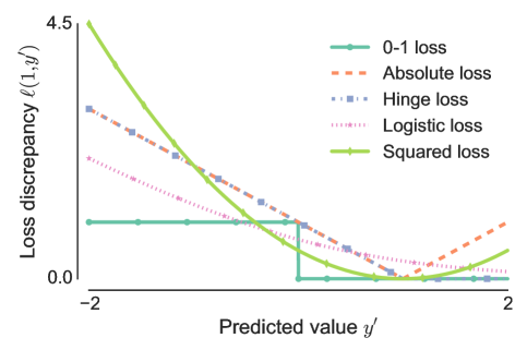
Figure 2.2: Loss discrepancies $\ell(1,y^{\prime})$ with $y=1$. (Adapted from Hastie et al. (2009))

4   Classes of supervised learning algorithms

Supervised learning aims at finding the best function $f$ in a hypothesis space $\mathcal{H}$ to model the input-output function of a system. If there is no restriction on the hypothesis space $\mathcal{H}$, the model $f$ can be any function $f\in\mathcal{Y}^{\mathcal{X}}$.

Consider a binary function $f$ which has $p$ binary inputs. The binary function is uniquely defined by knowing the output values of the $2^{p}$ possible input vectors. The hypothesis space of all binary functions contains $2^{2^{p}}$ binary functions. If we observe $n$ different input-output pair assignments, there remain $2^{2^{p}-n}$ possible binary functions. For a binary function of $p=5$ inputs, we have $2^{2^{5}}=4294967296$ possible binary functions. If we observe $n=16$ input-output pair assignments among the $2^{5}=32$ possible ones, we still have $2^{2^{5}-16}=65536$ possible binary functions. The number of possible functions highly increases with the cardinality of each variable. The hypothesis space will be even larger with a stochastic function, where different output values are possible for each possible input assignment.

By making assumptions on the model class $\mathcal{H}$, we can largely reduce the size of the hypothesis space. For instance in the previous example, if we assume that 2 out of the 5 binary input variables are independent of the output, there remain $2^{2^{3}}=256$ possible functions. The correct function would be uniquely identified by observing the $8$ possible assignments.

Given the data stochasticity, those model classes can directly model the input-output mapping $f:\mathcal{X}\rightarrow\mathcal{Y}$, but also the conditional probability $P(y|x)$ and predictions are made through

$$f(x)=\arg\min_{\hat{y}\in\mathcal{Y}}E_{y|x}\left[L(y,\hat{y})\right]=\arg\min_{\hat{y}}\int_{\mathcal{Y}}L(y,\hat{y})dP(y|x).$$ (2.2)

We will present some of the most popular model classes: linear models in Section 4.1; artificial neural networks in Section 4.2 which are inspired from the neurons in the brain; neighbors-based models in Section 4.3 which find the nearest samples in the training set; decision tree based-models in Section 4.4 (and in more details in Chapter 3). Note that we introduce ensemble methods in Section 4.4 and discuss them more deeply in Chapter 4.

4.1   Linear models

Let us denote by $x\in\mathbb{R}^{p}=\begin{bmatrix}x_{1}&\ldots&x_{p}\end{bmatrix}^{T}$ a vector of input variables. A linear model $\hat{f}$ is a model having the following form

$$\hat{f}(x)=\beta_{0}+\sum_{j=1}^{p}\beta_{j}x_{j}=\begin{bmatrix}1&x^{T}\end{bmatrix}\beta$$

where the vector $\beta\in\mathbb{R}^{1+p}$ is a concatenation of the intercept $\beta_{0}$ and the coefficients $\beta_{j}$.

Given a set of $n$ input-output pairs $\{(x^{i},y^{i})\in(\mathcal{X},\mathcal{Y})\}_{i=1}^{n}$, we retrieve the coefficient vector $\beta$ of the linear model by minimizing a loss $\ell:~\mathcal{Y}\times~\mathcal{Y}\rightarrow\mathbb{R}^{+}$:

$$\min_{\beta}\sum_{i=1}^{n}\ell(y^{i},\hat{f}(x^{i}))=\min_{\beta}\sum_{i=1}^{n}\ell(y^{i},\begin{bmatrix}1&{x^{i}}^{T}\end{bmatrix}\beta).$$ (2.3)

With the square loss $\ell(y,y^{\prime})=\frac{1}{2}(y-y^{\prime})^{2}$, there exists an analytical solution to Equation 2.3 called ordinary least squares. Let us denote by $\mathbf{X}\in\mathbb{R}^{n\times(1+p)}$ the concatenation of the input vectors with a first column of $\mathbf{X}$ full of ones to model the intercept $\beta_{0}$ and by $\mathbf{y}\in\mathbb{R}^{n}$ the concatenation of the output values. We can now express the sum of squares in matrix notation:

$$\sum_{i=1}^{n}\ell(y,\hat{f}(x^{i})) =\frac{1}{2}\sum_{i=1}^{n}(y^{i}-\hat{f}(x^{i}))^{2}$$ (2.4)

$$=\frac{1}{2}(\mathbf{y}-\mathbf{X}\beta)^{T}(\mathbf{y}-\mathbf{X}\beta)$$ (2.5)

The first order differentiation of the sum of squares with respect to $\beta$ yields to

$$\frac{\partial}{\partial\beta}\sum_{i=1}^{n}\ell(y,\hat{f}(x^{i}))=\mathbf{X}^{T}(\mathbf{y}-\mathbf{X}\beta).$$ (2.6)

The vector minimizing the square loss is thus

$$\beta=(\mathbf{X}^{T}\mathbf{X})^{-1}\mathbf{X}^{T}y.$$ (2.7)

The solution exists only if $\mathbf{X}^{T}\mathbf{X}$ is invertible.

Whenever the number of inputs plus one $p+1$ is greater than the number of samples $n$, the analytical solution is ill posed as the matrix $\mathbf{X}^{T}\mathbf{X}$ is rank deficient ($rank(\mathbf{X}^{T}\mathbf{X})<p+1$). To ensure a unique solution, we can add a regularization penalty $R$ with a multiplying constant $\lambda\in\mathbb{R}^{+}$ on the coefficients $\beta$ of the linear model:

$$\min_{\beta}\sum_{i=1}^{n}L(y^{i},\beta_{0}+\sum_{j=1}^{p}\beta_{j}x_{j}^{i})+\lambda R(\beta_{1},~\ldots,\beta_{p}).$$ (2.8)

With a $\ell_{2}$-norm constraint on the coefficients, we transform the ordinary least square model into a ridge regression model Hoerl and Kennard (1970):

$$\min_{\beta}\sum_{i=1}^{n}\left(y^{i}-\beta_{0}-\sum_{j=1}^{p}\beta_{j}x_{j}^{i}\right)^{2}+\lambda\sum_{j=1}^{p}\beta_{j}^{2}.$$ (2.9)

One can show (see Section 3.4.1 of Hastie et al. (2009)) that the constant $\lambda$ controls the maximal value of all coefficients $\beta_{j}$ in the ridge regression solution.

With a $\ell_{1}$-norm constraint ($R(\beta_{1},~\ldots,\beta_{p})=\sum_{j=1}^{p}|\beta_{j}|$) on the coefficient $\beta_{1},\ldots,\beta_{p}$, we have the Lasso model Tibshirani (1996b):

$$\min_{\beta}\sum_{i=1}^{n}\left(y^{i}-\beta_{0}-\sum_{j=1}^{p}\beta_{j}x_{j}^{i}\right)^{2}+\lambda\sum_{j=1}^{p}|\beta_{j}|.$$ (2.10)

Contrarily to the ridge regression, the Lasso has no closed formed analytical solution even though the resulting optimization problem remains convex. However, we gain that the $\ell_{1}$-norm penalty sparsifies the coefficients $\beta_{j}$ of the linear model. If the constant $\lambda$ tends towards infinity, all the coefficients will be zero $\beta_{j}=0$. While with $\lambda=0$, we have the ordinary least square formulation. With $\lambda$ moving from $+\infty$ to $0$, we progressively add variables to the linear model with a magnitude $\sum_{j=1}^{p}|\beta_{j}|$ depending on $\lambda$. The monotone Lasso Hastie et al. (2007) further restricts the coefficient to monotonous variation with respect to $\lambda$ and has been shown to perform better whenever the input variables are correlated.

A combination of the $\ell_{1}$-norm and the $\ell_{2}$-norm constraints on the coefficients is called an elastic net penalty Zou and Hastie (2005). It shares both the property of the Lasso and the ridge regression: sparsely selecting coefficients as in Lasso and considering groups of correlated variables together as in the ridge regression. With a careful design of the penalty term $R$, we can enforce further properties such as selecting variables in groups of pre-defined variables with the group Lasso Yuan and Lin (2006); Meier et al. (2008) or taking into account the variable locality in the coefficient vector $\beta$ while adding a new variable to the linear model with the fused Lasso Tibshirani et al. (2005).

By selecting an appropriate loss and penalty term, we have a wide variety of linear models at our disposal with different properties. In regression, an absolute loss leads to the least absolute deviation algorithm Bloomfield and Steiger (2012) which is robust to outliers. In classification, we can use a logistic loss to model the class probability distribution leading to the logistic regression model. With a hinge loss, we aim at finding a hyperplane which maximizes the separations between the classes leading to the support vector machine algorithm Cortes and Vapnik (1995).

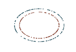
(a)

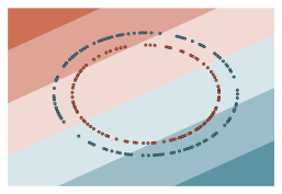
(b) Original input space

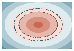
(c) Non-linear transformation

Figure 2.3: The logistic linear model on the bottom left is unable to find a separating hyperplane. If we fit the linear model on the distance from the center of circle, we separate perfectly both classes as shown in the bottom right.

A linear model can handle non linear problems by applying first a non linear transformation to the input space $\mathcal{X}$. For instance, consider the classification task of Figure 2.3a where each class is located on a concentric circle. Given the non linearity of the problem, we can not find a straight line separating both classes in the cartesian plane as shown in Figure 2.3b. If instead we fit a linear model on the distance from the origin $\sqrt{x_{1}^{2}+x_{2}^{2}}$ as illustrated in Figure 2.3c, we find a model separating perfectly both classes. We often use linear models in conjunction with kernel functions (presented in Section 8.3), which provide a range of ways to achieve non-linear transformations of the input space.

4.2   (Deep) Artificial neural networks

An artificial neural network is a statistical model mimicking the structure of the brain and composed of artificial neurons. A neuron, as shown in Figure 2.4a, is composed of three parts: the soma, the cell body, processes the information from its dendrites and transmits its results to other neurons through the axon, a nerve fiber. An artificial neuron follows the same structure (see Figure 2.4b) replacing biological processing by numerical computations. The basic neuron Rosenblatt (1958) used for supervised learning consists in a linear model of parameters $\beta\in\mathbb{R}^{p+1}$ followed by an activation function $\phi$:

$$\hat{f}_{neuron}(x)=\phi\left(\beta_{0}+\sum_{j=1}^{p}\beta_{j}x_{j}\right).$$

The activation function replicates artificially the non linear activation of real neurons. It is a scalar function such as a hyperbolic tangent $\phi(x)=\tanh(x)$, a sigmoid $\phi(x)=(1+e^{-x})^{-1}$ or a rectified linear function $\phi(x)=\max(0,x)$.

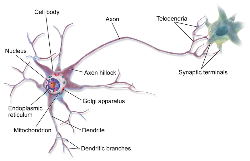
(a) Biological neuron

(b) Artificial neuron

Figure 2.4: A biological neuron (on the left) and an artificial neuron (on the right).

More complex artificial neural networks are often structured into layers of artificial neurons. The inputs of a layer are the input variables or the outputs of the previous layer. Each neuron of the layer has one output. The neural network is divided into three parts as in Figure 2.5: the first and last layers are respectively the input layer and the output layer, while the layers in between are the hidden layers. The hidden layer of Figure 2.5 is called a fully connected layer as all the neurons (here the input variables) from the previous layer are connected to each neuron of the layer. Other layer structures exist such as convolutional layers Krizhevsky et al. (2012); LeCun et al. (2004) which mimic the visual cortex Hubel and Wiesel (1968). A network is not necessarily feed forward, but can have a more complex topology for example recurrent neural networks Boulanger-Lewandowski et al. (2012); Graves et al. (2013) mimic the brain memory by forming internal cycles of neurons. Neural networks with many layers are also known LeCun et al. (2015) as deep neural networks.

Figure 2.5: A neural network with an input layer, a fully connected hidden layer and an output layer.

Artificial neurons form a graph of variables. Through this representation, we can learn such models by applying gradient based optimization techniques Bengio (2012); Glorot and Bengio (2010); LeCun et al. (2012) to find the coefficient vector associated to each neuron minimizing a given loss function.

4.3   Neighbors based methods

The $k$-nearest neighbors model is defined by a distance metric $d$ and a set of samples. At learning time, those samples are stored in a database. We predict the output of an unseen sample by aggregating the outputs of the $k$-nearest samples in the input space according to the distance metric $d$, with $k$ being a user-defined parameter.

More precisely, given a training set $\left((x^{i},y^{i})\in\left(\mathcal{X}\times\mathcal{Y}\right)\right)_{i=1}^{n}$ and a distance measure $d:\mathcal{X}\times\mathcal{X}\rightarrow\mathbb{R}^{+}$, an unseen sample with value in the input space $x$ is assigned a prediction through the following procedure:

1. Compute the distances $d(x^{i},x)$ in the input space, $\forall i=1,\ldots,n$, between the training samples $x^{i}$ and the input vector $x$.

2. Search for the $k$ samples in the training set which have the smallest distance to the vector $x$.

3. In classification, compute the proportion of samples of each class among these $k$-nearest neighbors: the final prediction is the class with the highest proportion. This corresponds to a majority vote over the $k$ nearest neighbors. In regression, the prediction is the average output of the $k$-nearest neighbors.

The $k$-nearest neighbor method adapts to a wide variety of scenarios by selecting or by designing a proper distance metric such as the euclidean distance or the Hamming distance.

4.4   Decision tree models

A decision tree model is a hierarchical set of questions leading to a prediction. The internal nodes, also called test nodes, test the value of a feature. In Figure 2.6, the starting node, also called root node, tests whether the feature “Petal width” is bigger or smaller than $0.7cm$. According to the answer, you follow either the right branch ($>0.7cm$) leading to another test node or the left branch ($\leq 0.7cm$) leading to an external node, also called a leaf. To predict an unseen sample, you start at the root node and follow the tree structure until reaching a leaf labelled with a prediction. With the decision tree of Figure 2.6, an iris with petal width smaller than $0.7cm$ is an iris Setosa.

Figure 2.6: A decision tree classifying iris flowers into its Setosa, Versicolor or Virginica varieties according to the width and length of its petals and sepals.

A classification or a regression tree Breiman et al. (1984) is built using all the input-output pairs $((x^{i},y^{i})\in(\mathcal{X}\times\mathcal{Y}))_{i=1}^{n}$ as follows: for each test node, the best split $(S_{r},S_{l})$ of the local subsample $S$ reaching the node is chosen among the $p$ input features combined with the selection of an optimal cut point. The best sample split $(S_{r},S_{l})$ of $S$ minimizes the average reduction of impurity

$$\Delta I((y^{i})_{i\in S},(y^{i})_{i\in S_{l}},(y^{i})_{i\in S_{r}})$$

$$=I((y^{i})_{i\in S})-\frac{|S_{l}|}{|S|}I((y^{i})_{i\in S_{l}})-\frac{|S_{r}|}{|S|}I((y^{i})_{i\in S_{r}}),$$ (2.11)

where $I$ is the impurity of the output such as the entropy in classification or the variance in regression. The decision tree growth continues until we reach a stopping criterion such as no impurity $I((y^{i})_{i\in S})=0$.

To avoid over-fitting, we can stop earlier the tree growth by adding further stopping criteria such as a maximal depth or a minimal number of samples to split a node.

Instead of a single decision tree, we often train an ensemble of such models:

• Averaging-based ensemble methods grow an ensemble by randomizing the tree growth. The random forest method Breiman (2001) trains decision trees on bootstrap copies of the training set, i.e. by sampling with replacement from the training dataset, and it randomizes the best split selection by searching this split among $k$ out of the $p$ features at each nodes ($k\leq p$).

• Boosting-based methods Freund and Schapire (1997); Friedman (2001) build iteratively a sequence of weak models such as shallow trees which perform only slightly better than random guessing. Each new model refines the prediction of the ensemble by focusing on the wrongly predicted training input-output pairs.

We further discuss decision tree models in Chapter 3 and ensemble methods in Chapter 4.

4.5   From single to multiple output models

With multiple outputs supervised learning tasks, we have to infer the values of a set of $d$ output variables $y_{1},\ldots,y_{d}$ (instead of a single one) from a set of $p$ input variables $x_{1},\ldots,x_{p}$. We hope to improve the accuracy and / or computational performance by exploiting the correlation structure between the outputs. There exist two main approaches to solve multiple output tasks: problem transformation presented in Section 4.5.1 and algorithm adaptation in Section 4.5.2. We present here a non exhaustive selection of both approaches. The interested reader will find a broader review of the multi-label literature in Zhang and Zhou (2014); Tsoumakas et al. (2009); Madjarov et al. (2012); Gibaja and Ventura (2014) and of the multi-output regression literature in Spyromitros-Xioufis et al. (2016); Borchani et al. (2015).

4.5.1   Problem transformation

The problem transformation approach transforms the original multi-output task into a set of single output tasks. Each of these single output tasks is then solved by classical classifiers or regressors. The possible output correlations are exploited through a careful reformulation of the original task.

Independent estimators

The simplest way to handle multi-output learning is to treat all outputs in an independent way. We break the prediction of the $d$ outputs into $d$ independent single output prediction tasks. A model is fitted on each output. At prediction time, we concatenate the predictions of these $d$ models. This is called the binary relevance method Tsoumakas et al. (2009) in multi-label classification and the single target method Spyromitros-Xioufis et al. (2016) in multi-output regression. Since we consider the outputs independently, we neglect the output correlation structure. Some methods may however benefit from sharing identical computations needed for the different outputs. For instance, the $k$-nearest neighbor method can share the search for the $k$-nearest neighbors in the input space, and the ordinary linear least squares method can share the computation of $(\mathbf{X}^{T}\mathbf{X})^{-1}\mathbf{X}^{T}$ in Equation 2.7.

Estimator chain

If the outputs are dependent, the model of a single output might benefit from the values of the correlated outputs. In the estimator chain method, we sequentially learn a model for each output by providing the predictions of the previously learnt models as auxiliary inputs. This is called a classifier chain Read et al. (2011) in classification and a regressor chain Spyromitros-Xioufis et al. (2016) in regression.

More precisely, the estimator chain method first generates an order $o$ on the outputs for instance based on prior knowledge, the output density, the output variance or at random. Then with the training samples and the output order $o$, it sequentially learns $d$ estimators: the $l$-th estimator $f_{o_{l}}$ aims at predicting the $o_{l}$-th output using as inputs the concatenation of the input vectors with the predictions of the models learnt for the $l-1$ previous outputs. To reduce the model variance, we can generate an ensemble of estimator chains by randomizing the chain order (and / or the underlying base estimator), and then we average their predictions.

In multi-label classification, Cheng et al. (2010) formulates a Bayes optimal classifier chain by modeling the conditional probability of $P_{\mathcal{Y}|\mathcal{X}}(y|x)$. Under the chain rule, we have

$$P_{\mathcal{Y}|\mathcal{X}}(y|x)=P_{\mathcal{Y}_{1}|\mathcal{X}}(y_{1}|x)\prod_{j=2}^{d}P_{\mathcal{Y}_{j}|\mathcal{X},\mathcal{Y}_{1},\ldots,\mathcal{Y}_{j-1}}(y_{j}|x,y_{1},\ldots,y_{j-1}).$$ (2.12)

Each estimator of the chain approximates a probability factor of the chain rule decomposition. Using the estimation of $P_{\mathcal{Y}|\mathcal{X}}$ made by the chain and a given loss function $\ell$, we can perform Bayes optimal prediction:

$$h^{*}(x)=\arg\min_{y^{\prime}}E_{\mathcal{Y}|\mathcal{X}}\ell(y^{\prime},y).$$ (2.13)

Error correcting codes

Error correcting codes are techniques from information and coding theory used to properly deliver a message through a noisy channel. It first codes the original message, and then corrects the errors made during the transmission at decoding time. This idea have been applied to multi-class classification Dietterich and Bakiri ; Guruswami and Sahai (1999), multi-label classification Ferng and Lin (2011); Zhang and Schneider (2011); Kajdanowicz and Kazienko (2012); Kouzani and Nasireding (2009); Guo et al. (2008); Hsu et al. (2009); Kapoor et al. (2012); Cisse et al. (2013) and multi-output regression Tsoumakas et al. (2014); Yu et al. (2006) tasks by viewing the predictions made by the supervised learning model(s) as a message transmitted through a noisy channel. It transforms the original task by encoding the output values with a binary error correcting code or output projections. One classifier is then fitted for each bit of the code or output projection. At prediction time, we concatenate the predictions made by each estimator and decode them by solving the inverse problem. Note that the output coding might also have for objective to reduce the dimensionality of the output space Hsu et al. (2009); Kapoor et al. (2012).

Pairwise comparisons

In multi-label tasks, the ranking by pairwise comparison approach Hüllermeier et al. (2008) aims to generate a ranking of the labels by making all the pairwise label comparisons. The original tasks is transformed into $d(d-1)/2$ binary classification tasks where we compare if a given label is more likely to appear than another label. The datasets comparing each label pair is obtained by collecting all the samples where only one of the outputs is true, but not both. This approach is similar to the one-versus-one approach Park and Fürnkranz (2007) in multi-class classification task, however we can not directly transform the ranking into a prediction, i.e. label set. To decrease the prediction time, alternative ranking construction schemes have been proposed Mencia and Fürnkranz (2008); Mencía and Fürnkranz (2010) requiring less than $d(d-1)/2$ classifier predictions.

The Calibrated label ranking method Brinker et al. (2006); Fürnkranz et al. (2008) extends the previous approach by adding a virtual label which will serve as a split point between the true and the false labels. For each label, we add a new tasks using all the samples comparing the label $i$ to the virtual label whose value is the opposite of the label $i$. To the $d(d-1)/2$ tasks, we effectively add $d$ tasks.

Label power set

For multi-label classification tasks, the label power set method Tsoumakas et al. (2009) encodes each label set in the training set as a class. It transforms the original task into a multi-class classification task. At prediction time, the class predicted by the multi-class classifier is decoded thanks to the one-to-one mapping of the label power set encoding. The drawback of this approach is to generate a large number of classes due to the large number of possible label sets. For $n$ samples and $d$ labels, the maximal number of classes is $\max(2^{d},n)$. This leads to accuracy issues if some label sets are not well represented in the training set. To alleviate the explosion of classes, rakel Tsoumakas and Vlahavas (2007) generates an ensemble of multi-class classifiers by subsampling the output space and then applying the label power set transformation.

4.5.2   Algorithm adaptation

The algorithm adaptation approach modifies existing supervised learning algorithms to handle multiple output tasks. We show here how to extend the previously presented models classes to multi-output regression and to multi-label classification tasks.

Linear-based models

Linear-based models have been adapted to multi-output tasks by reformulated their mathematical formulation using multi-output losses and (possibly) regularization constraints enforcing assumptions on the input-output and the output-output correlation structures. The proposed methods are based for instance on extending least-square regression Dayal and MacGregor (1997); Breiman and Friedman (1997); Similä and Tikka (2007); Baldassarre et al. (2012); Evgeniou et al. (2005); Zhou and Tao (2012) (with possibly regularization), canonical correlation analysis Izenman (1975); Van Der Merwe and Zidek (1980), support vector machine Elisseeff and Weston (2001); Jiang et al. (2008); Xu (2012); Evgeniou and Pontil (2004); Evgeniou et al. (2005), support vector regression Vazquez and Walter (2003); Sánchez-Fernández et al. (2004); Liu et al. (2009); Xu et al. (2013), and conditional random fields Ghamrawi and McCallum (2005).

(Deep) Artificial neural networks

Neural networks handles multi-output tasks by having one node on the output layer per output variable. The network minimizes a global error function defined over all the outputs Specht (1991); Zhang and Zhou (2006); Ciarelli et al. (2009); Zhang (2009); Nam et al. (2014). The output correlation are taken into account by sharing the input and the hidden layers between all the outputs.

Nearest neighbors

The $k$-nearest neighbors algorithm predicts an unseen sample $x$ by aggregating the output value of the $k$ nearest neighbors of $x$. This algorithm is adapted to multi-output tasks by sharing the nearest neighbors search among all outputs. If we just share the search, this is called binary relevance of $k$-nearest neighbors in classification and single target of $k$-nearest neighbors in regression. Multi-output extensions of the $k$-nearest neighbors modifies how the output values of the nearest neighbors are aggregated for the predictions for instance it can utilize the maximum a posteriori principle Zhang and Zhou (2007); Younes et al. (2011); Cheng and Hüllermeier (2009) or it can re-interpret the output aggregation as a ranking problem Chiang et al. (2012); Brinker and Hüllermeier (2007),

Decision trees

The decision tree model is a hierarchical structure partitioning the input space and associating a prediction to each partition. The growth of the tree structure is done by maximizing the reduction of an impurity measure computed in the output space. When the tree growth is stopped at a leaf, we associate a prediction to this final partition by aggregating the output values of the training samples. We adapt the decision tree algorithm to multi-output tasks in two steps Segal (1992); De’Ath (2002); Blockeel et al. (2000); Clare and King (2001); Zhang (1998); Vens et al. (2008); Noh et al. (2004): (i) multi-output impurity measures are used to grow the structure as the sum over the output space of the entropy or the variance; (ii) the leaf predictions are obtained by computing a constant minimizing a multi-output loss function such as the $\ell_{2}$-norm loss in regression or the Hamming loss in classification. We discuss in more details how to adapt the decision tree algorithm to multi-output tasks in Section 13.

Instead of growing a single decision tree, they are often combined together to improve their generalization performance. Random forest models Breiman (2001); Geurts et al. (2006a) averages the predictions of several randomized decision trees and has been studied in the context of multi-output learning Kocev et al. (2007); Segal and Xiao (2011); Kocev et al. (2013); Madjarov et al. (2012); Joly et al. (2014).

Ensembles

Ensemble methods aggregate the predictions of multiple models into a single one so to improve its generalization performance. We discuss how the averaging and boosting approaches have been adapted to multi-output supervised learning tasks.

Averaging ensemble methods have been straightforwardly adapted by averaging the prediction of multi-output models. Instead of averaging scalar predictions, it averages Kocev et al. (2007); Segal and Xiao (2011); Kocev et al. (2013); Madjarov et al. (2012); Joly et al. (2014) the vector predictions of each model of the ensemble. If the learning algorithm is not inherently multi-output, we could use one the problem transformation techniques as in rakel Tsoumakas and Vlahavas (2007), which uses the label power set transformation, or ensemble of estimator chain Read et al. (2011).

Boosting ensembles are grown by sequentially adding weak models minimizing a selected loss, such as the Hamming loss Schapire and Singer (2000), the ranking loss Schapire and Singer (2000), the $\ell_{2}$-norm loss Geurts et al. (2006b) or any differentiable loss function (see Chapter 6).

5   Evaluation of model prediction performance

For a given supervised learning model $f$ trained on a set of samples $\left((x^{i},y^{i})\in\left(\mathcal{X}\times\mathcal{Y}\right)\right)_{i=1}^{n}$, we want a model having good generalization able to predict unseen samples. Otherwise said, the model $f$ should have minimal generalization error over the input-output pair distribution, where the generalization error is defined as:

$$\text{Generalization error}=E_{P_{{\cal X},{\cal Y}}}\{\ell(f(x),y)\}$$ (2.14)

for a given loss function $\ell:\mathcal{Y}\times\mathcal{Y}\rightarrow\mathbb{R}^{+}$.

Evaluating Equation 2.14 is generally unfeasible, except in the rare cases where (i) the input-output distribution $P_{{\cal X},{\cal Y}}$ is fully known and (ii) for restricted classes of models. In practice, neither of these conditions are met. However, we still need a principle way to approximate the generalization error.

A first approach to approximate Equation 2.14 is to evaluate the error of the model $f$ on the training samples $\mathcal{L}=\left((x^{i},y^{i})\in\left(\mathcal{X}\times\mathcal{Y}\right)\right)_{i=1}^{n}$ leading to the resubstitution error:

$$\text{Resubstitution error}=\frac{1}{|\mathcal{L}|}\sum_{(x,y)\in\mathcal{L}}^{n}\ell(f(x),y)$$ (2.15)

A model with a high resubstitution error often has a high generalization error and indeed underfits the data. The linear model shown in Figure 2.7a underfits the data as it is not complex enough to fit the non linear data (here a second degree polynomial). Instead, we can fit a high order polynomial model to have a zero resubstitution error as illustrated in Figure 2.7b. This complex model has poor generalization error as it perfectly fits the noisy samples unable to retrieve the second order parabola. Such overly complex models with zero resubstitution error and non zero generalization error are said to overfit the data. Since a zero resubstitution error does not imply a low generalization error, it is a poor proxy of the generalization error.

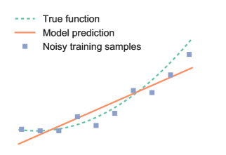
(a) Under-fitting

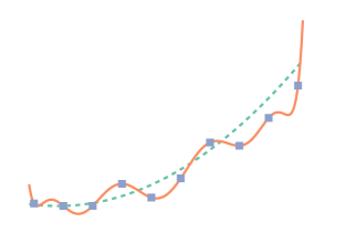
(b) Over-fitting

Figure 2.7: The linear model on the left figure underfits the training samples, while the high order polynomial model on the right overfits the training samples.

Since we assess the quality of the model with the training samples, the resubstitution error is optimistic and biased. Furthermore, it favors overly complex models (as depicted in Figure 2.7). To improve the approximation of the generalization error, we need to use techniques which avoid to use the training samples for performance evaluation. They are either based on sample partitioning methods, such as hold out methods and cross validation techniques, or sample resampling methods, such as bootstrap estimation methods. Since the amount of available data and time are fixed for both the model training and the model assessment, there is a trade-off between (i) the quality of the error estimate, (ii) the number of samples available to learn a model and (iii) the amount of computing time available for the whole process.

The hold out evaluation method splits the samples into a training set $LS$, also called learning set, and a testing set $TS$ commonly with a ratio of $2/3$ - $1/3$. The hold out error is given by

$$\text{Hold out error}=\frac{1}{|TS|}\sum_{(x,y)\in TS}\ell(f(x),y).$$ (2.16)

This methods requires a high number of samples as a large part of the data is devoted to the model assessment impeding the model training. If too few samples are allocated to the testing set, the hold out estimate becomes unreliable as its confidence intervals widen Kohavi et al. (1995). Since the hold out error is a random number depending on the sample partition, we can improve the error estimation by (i) generating $B$ random partitions $(LS_{b},TS_{b})_{b=1}^{B}$ of the available samples, (ii) fitting a model $f^{b}$ on each learning set $LS_{b}$ and (iii) averaging the performance of the $B$ models over their respective testing sets $TS_{b}$:

$$\text{Random subsampling error}=\frac{1}{B}\sum_{b=1}^{B}\frac{1}{|TS_{b}|}\sum_{(x,y)\in TS_{b}}\ell(f^{b}(x),y).$$ (2.17)

To improve the data usage efficiency, we can resort to cross-validation methods, also called rotation estimation, which split the samples into $k$ folds $\{TS_{1},\ldots,TS_{k}\}$ approximately of the same size. Cross validation methods average the performance of $k$ models $(f^{l})_{l=1}^{k}$ each tested on one of the $k$ folds and trained using the $k-1$ remaining folds:

$$\text{CV error}=\frac{1}{k}\sum_{l=1}^{k}\frac{1}{|TS_{l}|}\sum_{(x,y)\in TS_{l}}\ell(f^{l}(x),y).$$ (2.18)

The number of folds $k$ is usually $5$ or $10$. If $k$ is equal to the number of samples ($k=n$), it is called leave-one-out cross validation.

Given that the folds do not overlap for cross validation methods, we are tempted to assess the performance over the pooled cross validation estimates with a given $metric$ obtained by concatenating the predictions made by each model $f^{l}$ over each of the $k$-folds

$$\text{Pooled CV error}=metric\left((f^{1}(x),y)_{(x,y)\in TS_{1}}\frown\ldots\frown(f^{k}(x),y)_{(x,y)\in TS_{k}}\right),$$ (2.19)

where $\frown$ is the concatenation operator. There is no difference for sample-wise losses such as the square loss. However, this is not the case for metrics comparing a whole set of predictions to their ground truth. Depending on the metrics, it has been showed that pooling may or may not biase the error estimation Parker et al. (2007); Forman and Scholz (2010); Airola et al. (2011).

We can improve the quality of the estimate by repeating the cross validation procedures over $B$ different $k$-fold partitions, averaging the performance of the models $f^{b,l}$ over each associated testing set $TS_{b,l}$:

$$\text{Repeated CV error}=\frac{1}{Bk}\sum_{b=1}^{B}\sum_{l=1}^{k}\frac{1}{|TS_{b,l}|}\sum_{(x,y)\in TS_{b,l}}\ell(f^{b,l}(x),y).$$ (2.20)

If all combinations are tested exhaustively as in the leave-one-out case, it is called complete cross validation. Since it is often too expensive Kohavi et al. (1995), we can instead draw several sets of folds at random.

The bootstrap method Efron (1983) draws $B$ bootstrap datasets $\{B_{1},\ldots,B_{B}\}$ by sampling with replacement $n$ samples from the original dataset of size $n$. Each samples has a probability of $1-(1-\frac{1}{n})^{n}$ to be selected in a bootstrap which is approximately $0.632$ for large $n$. A first approach to estimate the error is to train a model $f^{b}$ on each bootstrap dataset and use the original dataset as a testing set:

$$\text{Bootstrap error}=\frac{1}{nB}\sum_{b=1}^{B}\sum_{(x,y)\in B_{b}}\ell(f^{b}(x),y).$$ (2.21)

This leads to over optimistic results, given the overlap between the training and the test data.

A better approach (discussed in Chapter 7.11 of Hastie et al. (2009)) is to imitate cross validation methods by fitting on each bootstrap dataset a model $f^{b}$ and using the unused samples as a testing set. This approach is called bootstrap leave-one-out:

$$\text{LOO Bootstrap error}=\frac{1}{n}\sum_{i=1}^{n}\frac{1}{|C^{-i}|}\sum_{b\in C^{-i}}\ell(f^{b}(x^{i}),y^{i}),$$ (2.22)

where $C^{-i}$ gives the bootstrap indices where the sample $i$ was not drawn. It is similar to a 2-fold repeated cross validation or random subsampling error with a ratio of 2/3 - 1/3 for the training and testing set. The estimation is thus biased as it uses approximately $0.632n$ training samples instead of $n$. We can alleviate this bias due to the sampling procedure through the “0.632” estimator which averages the training error and LOO Bootstrap error:

$$\text{0.632 estimator}= 0.632\times\text{LOO Bootstrap error}$$

$$+0.368\times\text{Resubstitution error}.$$ (2.23)

Note that with very low sample size, it has been shown Braga-Neto and Dougherty (2004) that the bootstrap approach yields better error estimate than the cross validation approach.

Until now, we have assumed that the samples are independent and identically distributed. Whenever this is no longer true, such as with time series of measurements, we have to modify the assessment procedure to avoid biasing the error estimation. For instance, the hold out estimate would train the model on the oldest samples and test the model on the more recent samples. Similarly in the medical context if we have several samples for one patient, we should keep these samples together in the training set or in the testing set.

Partition-based methods (hold out, cross validation) break the assumption in classification that the samples from the training set are independent from the samples in the testing set as they are drawn without replacement from a pool of samples. The representation of each class in the testing set is thus not guaranteed to be the same as in the training set. It is advised Kohavi et al. (1995) to perform stratified splits by keeping the same proportion of classes in each set.

6   Criteria to assess model performance

Assessing the performance of a model requires evaluation metrics which will compare the ground truth to a prediction, a score or a probability estimate. The selection of an appropriate scoring or error measure is essential and is dependent of the supervised learning task and the goal behind the modeling.

A first approach to assess a model is to define a goal for the model and to quantify its realization. For instance, a company wants to maximize its benefits and consider that the revenue must exceed the data analysis cost of gathering samples, fitting a model and exploiting its predictions. Unfortunately, this model optimization criterion is hardly expressible into economical terms. We could instead consider the effectiveness of the model such as the click-through-rate, used by online advertising companies, which counts the number of clicks on a link to the number of opportunities that users have to click on this link. However, it is hard to formulate a model optimizing directly this score and it requires to put the model into a production setting (or at least simulate its behavior). Other optimization criteria exit that are more amenable to mathematical analysis and numerical computation such as the square loss or the logistic loss. Knowing the properties of such criteria is necessary to make a proper choice.

We present binary classification metrics in Section 6.1. Then, we show how to extend these metrics to multi-class classification tasks in Section 6.2 and to multi-label classification tasks in Section 6.3. We introduce metrics for regression tasks and multi-output regression tasks in Section 6.4.

More details or alternative descriptions of these metrics can be found in the following references Sokolova and Lapalme (2009); Hossin and Sulaiman (2015); Ferri et al. (2009). Note that I made significant contributions to the implementations and the documentations of these metrics in the scikit-learn library Pedregosa et al. (2011); Buitinck et al. (2013).

6.1   Metrics for binary classification

Given a set of $n$ ground truth values $(y^{i}\in~\{0,1\})_{i=1}^{n}$ and their associated model predictions $(\hat{y}^{i}\in~\{0,1\})_{i=1}^{n}$, we can distinguish in binary classification four categories of predictions (as shown in Table 2.4). We denote by true positives (TP) and true negatives (TN) the predictions where the model accurately predicts the target respectively as true or false:

$$TP =\sum_{i=1}^{n}1(y^{i}=1;\hat{y}^{i}=1),$$ (2.24)

$$TN =\sum_{i=1}^{n}1(y^{i}=0;\hat{y}^{i}=0).$$ (2.25)

Whenever the model wrongly predicts the samples, we call false positives (FP) samples predicted as true while their labels are false and false negatives (FN) samples predicted as false while their labels are true:

$$FN =\sum_{i=1}^{n}1(y^{i}=1;\hat{y}^{i}=0),~$$ (2.26)

$$FP =\sum_{i=1}^{n}1(y^{i}=0;\hat{y}^{i}=1).$$ (2.27)

Together, the true positive, true negatives, false negatives and false positives form the so called confusion or contingency matrix shown in Table 2.4.

Table 2.4: For a binary classification task, the prediction of a model is divided into fours categories leading to a confusion matrix.

	Truly positive	Truly negative
Predicted positive	True positive	False positive
Predicted negative	False negative	True negatives

Two common metrics to assess classification performance are the error rate, the average of the $0-1$ loss, and its complement the accuracy:

Error rate $$=\frac{1}{n}\sum_{i=1}^{n}1(y^{i}\not=\hat{y}^{i}),$$ (2.28)

Accuracy $$=1-\text{Error rate}=\frac{1}{n}\sum_{i=1}^{n}1(y^{i}=\hat{y}^{i}).$$ (2.29)

Both metrics can be expressed in term of the confusion matrix:

Error rate $$=\frac{FP+FN}{n},$$ (2.30)

Accuracy $$=\frac{TN+TP}{n}.$$ (2.31)

The error rate does not distinguish the false negatives from the false positives. Similarly, the accuracy does not differentiate true positives from true negatives. Thus, two classifiers may have exactly the same accuracy or error rate, while leading to a totally different outcome by increasing either the number of misses (false negatives) or the number of false alarms (false positives). Furthermore, the error rate and the accuracy can be overly optimistic whenever there is a high class imbalance. A classification task with $99.99\%$ of samples in one of the classes would easily lead to an accuracy of $99.99\%$ (and an error rate of $0.01\%$) by alway predicting the most common class. The choice of an appropriate metric thus depends on the properties of the classification task, such as the class imbalance.

To differentiate false positives from false negative, we can assess separately the proportion of correctly classified positive and negative samples. This leads to the true positive rate (resp. true negative rate) which computes the proportion of correctly classified positive (resp. negative) samples:

True positive rate $$=\frac{TP}{TP+FN}$$ (2.32)

True negative rate $$=\frac{TN}{TN+FP}$$ (2.33)

The complement of the true positive rate (resp. true negative rate) is the false negative rate (resp. false positive rate):

False negative rate $$=1-\text{True positive rate}=\frac{FN}{TP+FN},$$ (2.34)

False positive rate $$=1-\text{True negative rate}=\frac{FP}{TN+FP}.$$ (2.35)

The true positive rate is also called sensitivy and tests the ability of the classifier to correctly classify all positive samples as true. A test with $100\%$ sensitivity implies that all positive samples are correctly classified. However, this does not imply that all samples are correctly classified. A classifier predicting all samples as true leads to $100\%$ sensitivity and totally neglects false positives. We have to look to the true negative rate, also called specifity, which tests the ability of the classifier to correctly classify all negative samples as negative. A perfect classifier should thus have a high sensitivity and a high specifity. In the medical domain, the sensitivity and the specificity are often used to characterize and to choose the behavior of diagnosis tests such as pregnancy tests.

The average of the specifity and sensitivity is called the balanced accuracy:

Balanced accuracy $$=\frac{\text{True positive rate}+\text{True negative rate}}{2}$$ (2.36)

$$=\frac{\text{specifity}+\text{sensitivty}}{2}$$ (2.37)

$$=\frac{1}{2}\frac{TP}{TP+FN}+\frac{1}{2}\frac{TN}{TN+FP}.$$ (2.38)

In the information retrieval context, a user sets a query to an information system, e.g. a web search engine, to detect which documents are relevant among a collection of such documents. In such systems, the collection of documents is often extremely large with only a few relevant documents to a given query. Due to the small proportion of relevant documents, we want to maximize the precision, the fraction of correctly predicted documents among the predicted documents. Binary classification tasks with a high class imbalance can be viewed as an information retrieval problems. In the context of binary classification tasks, the precision is expressed as

$$\text{Precision}=\frac{TP}{TP+FP},$$ (2.39)

To have a perfect precision, one could predict all documents or samples as negative (as irrelevant documents). In parallel, we want also to maximize the recall, the proportion of correctly predicted true samples among the true samples. The recall is a synonym for true positive rate and sensitivity.

The precision and recall are often combined into a single number by computing the $F_{1}$ score, the harmonic mean of the precision and recall,

$$F_{1}=\frac{2}{\frac{1}{\text{Precision}}+\frac{1}{\text{Recall}}}.$$ (2.40)

Some classifiers associate a score or a probability $\hat{f}(x)$ to a sample instead of a class label. We can threshold these continuous predictions by a constant $\tau$ to compute the number of true positives, false positives, false negatives and true negatives:

$$TP(\tau) =\sum_{i=1}^{n}1(y^{i}=1;f(x^{i})\geq\tau),$$ (2.41)

$$TN(\tau) =\sum_{i=1}^{n}1(y^{i}=0;f(x^{i})\leq\tau),$$ (2.42)

$$FN(\tau) =\sum_{i=1}^{n}1(y^{i}=0;f(x^{i})\geq\tau),~$$ (2.43)

$$FP(\tau) =\sum_{i=1}^{n}1(y^{i}=1;f(x^{i})\leq\tau).$$ (2.44)

By varying $\tau$, we can first derive performance curves to analyze the prediction performance of those more models and then select a classifier performance point with pre-determined classification performance.

The receiver operating characteristic (ROC) curve Fawcett (2006) plots the true positive rate as a function of the false positive rate by varying the threshold $\tau$ as shown in Figure 2.8a. The receiver, the model user, can indeed choose any point on the curve to operate at a given model specifity / sensitivity tradeoff. A random estimator has its performance on the line $((0,0),(1,1))$, while a perfect classifier has the points $(0,1)$ with $0\%$ of false positive rate and $100\%$ of true positive rate on its curve. Any curve below the random line can be reversed symmetrically to the line $((0,0),(1,1))$ by flipping the classifier prediction. The ROC curve is often used in the clinical domain Metz (1978) and coupled to a cost analysis to determine the proper threshold $\tau$. The area under the ROC curve can be interpreted as Hanley and McNeil (1982) the probability to rank with a higher score one true sample than one false sample chosen at random.

The precision-recall (PR) curve is the precision as a function of the recall as shown in Figure 2.8b. The ROC curve and the PR curves are linked as there is a one to one mapping between points in the ROC space and in the precision-recall space Davis and Goadrich (2006). However conversely to the ROC curve, the precision recall curve is sensitive to the class imbalance between the positive and negative classes. Since both the precision and recall do not take into account the amount of true negatives, the precision-recall curve (compared to the ROC curve) focuses on how well the estimator is able to classify correctly the positive class.

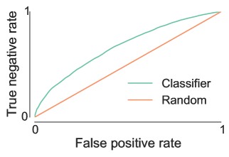
(a) ROC curve

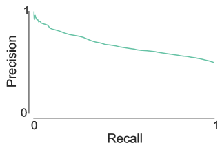
(b) PR curve

Figure 2.8: A receiver operating characteristic curve and a precision-recall curve of a classifier and a random model.

6.2   Metrics for multi-class classification

From binary classification to multi-class classification, the output value is no more restricted to two classes and can go up to $k$-classes. Given the ground truths $(y^{i}\in~\{1,...,k\})_{i=1}^{n}$ and the associated model predictions $(\hat{y}^{i}\in~\{1,...,k\})_{i=1}^{n}$, we can now divide the model predictions into $k^{2}$ categories leading to a $k\times k$ confusion matrix:

$$c_{l_{1},l_{2}}=\sum_{i=1}^{n}1(y^{i}=l_{1};\hat{y}^{i}=l_{2})\quad\forall l_{1},l_{2}\in\{1,...,k\}.$$ (2.45)

Metrics such as the accuracy, the error rate or the log loss (see Table 2.3) naturally extend to multi-class classification tasks. To extend other binary classification metrics (such as those developed in Section 6.1), we need to break the $k\times k$ confusion matrix into a set of $2\times 2$ confusion matrices.

A first approach is to consider that each class $l$ is in turns the positive class while the remaining labels form together the negative class. We thus have $k$ confusion matrices whose true positives $TP_{l}$, true negatives $TN_{l}$, false negatives $FN_{l}$ and false positives $FP_{l}$ for the class $l\in\{1,\ldots,k\}$ are

$$TP_{l} =c_{l,l},$$ (2.46)

$$TN_{l} =\sum_{j=1,j\not=l}^{k}c_{j,j},$$ (2.47)

$$FN_{l} =\sum_{j=1,j\not=l}^{k}c_{j,k},~$$ (2.48)

$$FP_{l} =\sum_{j=1,j\not=l}^{k}c_{k,j}.$$ (2.49)

By averaging a metric $M$ computed on each derived confusion matrix, we have the so called macro-averaged Sokolova and Lapalme (2009) of the corresponding binary classification metric

$$macro-M=\frac{1}{k}\sum_{l=1}^{k}M(TP_{l},TN_{l},FN_{l},FP_{l}).$$

Note that the balanced accuracy in binary classification is thus equal to the macro-specificity or macro-sensitivity in multi-class classification.

Another useful averaging is the micro-averaging Sokolova and Lapalme (2009). It uses as true positives $TP_{\mu}$ and true negatives $TN_{\mu}$ the sum of the diagonal elements of the confusion matrix and as false negatives $FN_{\mu}$ (resp. false positives $FP_{\mu}$) the sum of the lower (resp. upper) triangular part of the confusion matrix:

$$TP_{\mu} =\sum_{l=1}^{k}c_{l,l},$$ (2.50)

$$TN_{\mu} =\sum_{l=1}^{k}c_{l,l},$$ (2.51)

$$FN_{\mu} =\sum_{l=1}^{k}\sum_{j=1:j<l}^{k}c_{l,j},~$$ (2.52)

$$FP_{\mu} =\sum_{l=1}^{k}\sum_{j=1:j>l}^{k}c_{l,j}).$$ (2.53)

Each averaging has its own properties: the macro-averaging considers that each class has the same importance and the micro-averaging reduces the importance given to the minority classes.

6.3   Metrics for multi-label classification and ranking

From binary to multi-label classification, the ground truths $(y^{i}\in\{0,1\}^{d})_{i=1}^{n}$ and the model predictions $(\hat{y}^{i}\in\{0,1\}^{d})_{i=1}^{n}$ are no longer scalars, but vectors of size $d$ or label sets. Both representations are interchangeable. Usually, the number of labels associated to a sample is small compared to the total number of labels.

The accuracy Ghamrawi and McCallum (2005), also called subset accuracy, has a direct extension in multi-label classification

$$\text{Accuracy}=\frac{1}{n}\sum_{i=1}^{n}1(y^{i}=\hat{y}^{i}),$$ (2.54)

and requires for each prediction that the predicted label set matches exactly the ground truth. This is an overly pessimistic metric, especially for high dimensional label space, as it penalizes any single mistake made for one sample. The complement of the subset accuracy is called the subset 0-1 loss .

In information theory, the Hamming distance compares the number of differences between two coded messages. The Hamming error metric Schapire and Singer (1999) averages the Hamming distance between the ground truth and the model prediction over the samples

$$\text{Hamming error}=\frac{1}{n}\frac{1}{d}\sum_{i=1}^{n}\sum_{j=1}^{d}1(y^{i}_{j}\not=\hat{y}^{i}_{j}).$$ (2.55)

By contrast to the subset accuracy, the Hamming error is an optimistic metric when the label space is sparse. For a sufficiently large number of samples and a label density $\epsilon\rightarrow 0$, a (useless) model predicting always the presence of a label if its frequency of apparition is higher than $0.5$ in the training set will roughly have a Hamming error of $\epsilon$. In some situations, the label density $\epsilon$ is so small that (more useful) models have hardly an Hamming error lower than $\epsilon$.

Both the Hamming error and the subset accuracy ignore the sparsity of the label space leading to either overly optimistic or pessimistic error. Multi-label metrics should be aware of the label space sparsity.

In statistics, the Jaccard index $J$ or Jaccard similarity coefficient computes the similarity between two sets. Given two sets $A$ and $B$, the Jaccard index is defined as

$$J(A,B)=\frac{|A\cap B|}{|A\cup B|} \text{ with }J(\emptyset,\emptyset)=1.$$ (2.56)

With label sets encoded as boolean vectors $x,y\in\{0,1\}^{d}$, the Jaccard index becomes

$$J(x,y)=\frac{x^{T}y}{1_{d}^{T}x+1_{d}^{T}y-x^{T}y},$$ (2.57)

where $1_{d}$ is a vector of ones of size $d$. The Jaccard similarity score Godbole and Sarawagi (2004), also sometimes called accuracy, averages over the samples the Jaccard index between the ground truths and the model predictions:

$$\text{Jaccard similarity score}=\frac{1}{n}\sum_{i=1}^{n}J(y^{i},\hat{y}^{i}).$$ (2.58)

By contrast to the Hamming loss, the Jaccard similarity score puts more emphasis on the labels in the ground truth and the ones predicted by the models. Moreover, it totally ignores all the negative labels. The Jaccard similarity score can be viewed as “local” measure of similarity and the Hamming loss a “global” measure of distance.

A fitted model $f$ applied to an input vector $x$ can go beyond label prediction and associate to each label $j$ a score or a probability estimate $f(x)_{j}$. When the density of the label space $\epsilon$ is small and the size of the label space $d$ is very high, it is often hard to correctly predict all labels. Instead, the classifier can rank or score all the labels. We developed here metrics for such classifiers with different possible goals, e.g. to predict correctly the label with the highest score $f(x)_{j}$.

Note that in the following, we use indifferently the notation $|\cdot|$ to express the cardinality of a set or the $\ell_{1}$-norm of a vector.

If only the top scored label has to be correctly predicted, we are minimizing the one errorSchapire and Singer (1999) which computes the fraction of labels with the highest score or probability that are incorrectly predicted:

$$\text{One error}=\frac{1}{n}\sum_{i=1}^{n}I\left(y^{i}_{j}\not=1:j=\arg\max_{j\in\{1,\ldots,d\}}f(x^{i})_{j}\right).$$ (2.59)

If we want to discover all the true labels at the expense of some false labels, the coverage error Schapire and Singer (2000) is the metrics to minimize. It counts the average number of labels with the highest scores or probabilities to consider to cover all true labels:

$$\text{Coverage error}=\frac{1}{n}\sum_{i=1}^{n}\max_{j:y^{i}_{j}\not=1}\left|\left\{k:f(x^{i})_{k}\geq f(x^{i})_{j}\right\}\right|.$$ (2.60)

For a label density of $\epsilon$, the best coverage error is thus $\epsilon d$ and the worst is $d$.

If we want to ensure that pairwise label comparisons are correctly made by the classifier, we will minimize the (pairwise) ranking loss metrics Schapire and Singer (1999). It counts for each sample the number of wrongly made pairwise comparisons divided by the number of true labels and false labels

$$\text{Ranking loss}=\frac{1}{n}\sum_{i=1}^{n}\frac{1}{|y^{i}|}\frac{1}{d-|y^{i}|}\left|\left\{(k,l):f(x^{i})_{k}<f(x^{i})_{l},y^{i}_{k}=1,y^{i}_{l}=0\right\}\right|$$ (2.61)

The ranking loss is between $0$ and $1$. A ranking loss of $0$ (resp. $1$) indicates that all pairwise comparisons are correct (resp. wrong).

If we want that the classifier gives on average a higher score to true labels, we will use the label ranking average precision metric Schapire and Singer (2000) to assess the accuracy of the models. For each samples $y^{i}$, it averages over each true labels $j$ the ratio between (i) the number of true label (i.e. $y^{i}=1$) with higher scores or probabilities than the label $j$ to (ii) the number of labels ($y^{i}$) with higher score $f(x^{i})$ than the label $j$. Mathematically, we average the LRAP of all pairs of ground truth $y^{i}$ and its associated prediction $f(x^{i})$:

$$\text{LRAP}(\hat{f})=\frac{1}{|TS|}\sum_{i=1}^{n}\frac{1}{|y^{i}|}\sum_{j\in\{k:y^{i}_{k}=1\}}\frac{|\mathcal{L}_{j}^{i}(y^{i})|}{|\mathcal{L}_{j}^{i}(1_{d})|},$$ (2.62)

where

$$\mathcal{L}^{i}_{j}(q)=\left\{k:q_{k}=1\mbox{\leavevmode\nobreak\ and\leavevmode\nobreak\ }\hat{f}(x^{i})_{k}\geq\hat{f}(x^{i})_{j}\right\}.$$

The best possible average precision is thus 1. Note that the LRAP score is equal to fraction of positive labels if all labels are predicted with the same score or all negative labels have a score higher than the positive one.

Let us illustrate the computation of the previous metrics with a numerical example. We compare the ground truth $\mathbf{y}$ of $n=2$ samples in a label of size $d=5$ to the probability score $\mathbf{f(x)}$ given by the classifier:

$$\mathbf{y} =\begin{bmatrix}1&0&1&0&0\\ 1&0&0&0&0\end{bmatrix},$$

$$\mathbf{f(x)} =\begin{bmatrix}0.75&0.6&0.1&0.8&0.15\\ 0.25&0.8&0.1&0.15&0.3\end{bmatrix}.$$

Thresholding $\mathbf{f(x)}$ at 0.5 yields the prediction $\mathbf{\hat{y}}$ of the classifier:

$$\hat{y} =f(x)\leq 0.5\begin{bmatrix}1&1&0&1&0\\ 0&1&0&0&0\end{bmatrix}$$

Here, you will find the detailed computation of all previous metrics:

Accuracy $$=0+0=0,$$

Hamming loss $$=\frac{1}{2}\frac{1}{5}5=0.5,$$

Jaccard similarity score $$=\frac{1}{2}\left(\frac{1}{4}+\frac{0}{2}\right)=0.125,$$

Top error $$=\frac{1}{2}\left(1+1\right)=2,$$

Coverage error $$=\frac{5+3}{2}=4$$

Ranking loss $$=\frac{1}{2}\left(\frac{1}{2}\frac{1}{3}(1+3)+\frac{1}{4}\frac{1}{1}2\right)\approx 0.583,$$

LRAP $$=\frac{1}{2}\left(\frac{1}{2}(\frac{1}{2}+\frac{2}{5})+\frac{1}{1}\frac{1}{3}\right)\approx 0.392.$$

While the previous metrics are suited to assess multi-label classification models, we can complement these metrics with those developed for binary classification tasks, e.g. specifity, precision, ROC AUC,…(see Section 6.1). They are well understood in their respective domains and have attractive properties such as a good handling of class imbalance. We extend those metrics in three steps: (i) we break the ground truth and the model prediction vectors into its elements, (ii) we concatenate the elements into groups such as all predictions associated to a given sample or all samples associated to a given label and (iii) we average the binary classification metrics over each group. We will focus here on three averaging methods: macro-averaging, micro-averaging and sample-averaging. Each averaging method stems from a vision and different sets of assumptions.

If we view the multi-label classification task as a set of independent binary classification tasks, we compute the metrics $M$ over each output separately and average the performance over all $d$ labels leading the macro-averaging version Yang (1999) of the metrics $M$:

$$\text{macro-}M((y^{i})_{i=1}^{n},(\hat{y}^{i})_{i=1}^{n})=\frac{1}{d}\sum_{j=1}^{d}M((y^{i}_{j})_{i=1}^{n},(\hat{y}^{i}_{j})_{i=1}^{n})).$$ (2.63)

If instead we view each sample as the result of a query (like in a search engine), we want to evaluate the quality of each query (or sample) separately. Under this perspective, the sample-averaging approach Godbole and Sarawagi (2004) computes and averages the metric $M$ over each sample separately:

$$\text{sample-}M((y^{i})_{i=1}^{n},(\hat{y}^{i})_{i=1}^{n})=\frac{1}{n}\sum_{i=1}^{n}M(y^{i},\hat{y}^{i}).$$ (2.64)

The micro-averaging approach Yang (1999) views all label-sample pairs as forming an unique binary classification task. It compute the metric $M$ as if all label predictions were independent:

$$M\text{-micro}((y^{i})_{i=1}^{n},(\hat{y}^{i})_{i=1}^{n})=M((y^{i}_{j})_{i,j=(1,\ldots,n)},(\hat{y}^{i}_{k})_{i,j=(1,\ldots,n)})).$$ (2.65)

6.4   Regression metrics

Given a set of $n$ ground truths $(y^{i}\in\mathbb{R})_{i=1}^{n}$ and their associated model predictions $(\hat{y}^{i}\in\mathbb{R})_{i=1}^{n}$, regression tasks are often assessed using the mean square error (MSE), the average of the square loss, expressed by

$$\text{MSE}=\frac{1}{n}\sum_{i=1}^{n}\left(y^{i}-\hat{y}^{i}\right)^{2}.$$ (2.66)

From the mean square error, we can derive the $r^{2}$ score, also called the coefficient of determination. It is the fraction of variance explained by the model:

$$r^{2} =1-\frac{\text{MSE}}{\text{Output variance}}$$ (2.67)

$$=1-\frac{\sum_{i=1}^{n}(y^{i}-\hat{y}^{i})^{2}}{\sum_{i=1}^{n}(y^{i}-\frac{1}{n}\sum_{l=1}^{n}y^{l})^{2}}$$ (2.68)

The $r^{2}$ score is normally between 0 and 1. A $r^{2}$ score of zero indicates that the models is no better than a constant, while a $r^{2}$ of one indicates that the model perfectly explains the output given the inputs. A negative $r^{2}$ score might occur and it indicates that the model is worse than a constant model.

Square-based metrics are highly sensitive to the presence of outliers with abnormally high prediction errors. The mean absolute error (MAE), the average of the absolute loss, is often suggested as a robust replacement of the MSE:

$$\text{MAE}=\frac{1}{n}\sum_{i=1}^{n}|y^{i}-\hat{y}^{i}|.$$ (2.69)

These single output metrics naturally extend to multi-output regression tasks. The multi-output mean squared error and mean absolute error for an output space size $d$ is given by

MSE $$=\frac{1}{n}\frac{1}{d}\sum_{i=1}^{n}||y^{i}-\hat{y}^{i}||_{\ell_{2}}^{2},$$ (2.70)

MAE $$=\frac{1}{n}\frac{1}{d}\sum_{i=1}^{n}||y^{i}-\hat{y}^{i}||_{\ell_{1}}.$$ (2.71)

These measures average the metrics over all outputs assuming they are independent.

Similarly, averaging the $r^{2}$ score over each output leads to the macro-$r^{2}$ score:

$$\text{macro-}r^{2}=1-\frac{1}{d}\sum_{j=1}^{d}\frac{\sum_{i=1}^{n}(y^{i}_{j}-\hat{y}^{i}_{j})^{2}}{\sum_{i=1}^{n}(y^{i}_{j}-\frac{1}{n}\sum_{l=1}^{n}y^{l}_{j})^{2}}.$$ (2.72)

An alternative extension of the $r^{2}$ score is to consider the total fraction of the output variance, or more strictly the sum of the variance over each output, explained by the model

$$\text{variance-}r^{2} =1-\frac{MSE}{\text{Total output variance}}$$ (2.73)

$$=1-\frac{\sum_{i=1}^{n}||y^{i}-\hat{y}^{i}||_{\ell_{2}}^{2}}{\sum_{i=1}^{n}||y^{i}-\frac{1}{n}\sum_{l=1}^{n}y^{l}||_{\ell_{2}}^{2}},$$ (2.74)

which is equal to 1 minus the fraction of explained variance Bakker and Heskes (2003).

The variance-$r^{2}$ is a variance weighted average of the $r^{2}$ score. We can reformulate the variance-$r^{2}$ as:

$$\text{variance-}r^{2} =1-\frac{\sum_{i=1}^{n}\sum_{j=1}^{d}(y^{i}_{j}-\hat{y}^{i}_{j})^{2}}{\text{Total output variance}}$$ (2.75)

$$=1-\sum_{j=1}^{d}w_{j}\frac{\sum_{i=1}^{n}(y^{i}_{j}-\hat{y}^{i}_{j})}{\sum_{i=1}^{n}(y^{i}_{j}-\frac{1}{n}\sum_{l=1}^{n}y^{l})^{2}}$$ (2.76)

with $w_{j}=\frac{\sum_{i=1}^{n}(y^{i}_{j}-\frac{1}{n}\sum_{l=1}^{n}y^{l}_{j})^{2}}{\text{Total output variance}}$. By contrast, the macro-$r^{2}$ score would have uniform weights $w_{j}=\frac{1}{d}\,\forall j$ in Equation 2.76.

7   Hyper-parameter optimization

Supervised learning algorithms can be viewed as a function $A:(\mathcal{X}\times\mathcal{Y})_{i=1}^{n}\times\mathcal{A}\rightarrow\mathcal{H}$ taking as input a learning set $\mathcal{L}=\left((x^{i},y^{i})\in\left(\mathcal{X}\times\mathcal{Y}\right)\right)_{i=1}^{n}$ and a set of hyper-parameters $\alpha\in\mathcal{A}$ and outputting a function $f$ in a hypothesis space $\mathcal{H}\subset\mathcal{Y}^{\mathcal{X}}$. The hypothesis space $\mathcal{A}$ is defined through one or several hyper-parameter variables that can be either discrete, like the number of neighbors for a nearest neighbors model, or continuous, like the multiplying constant of a penalty loss in penalized linear models.

We need hyper-parameter tuning methods to find the best hyper-parameter set $\alpha^{*}\in\mathcal{A}$ that minimizes the expectation of some loss function $\ell:\mathcal{Y}\times\mathcal{Y}\rightarrow\mathbb{R}^{+}$ over the joint distribution of input / output pairs $P_{{\cal X},{\cal Y}}$:

$$\alpha^{*}=\arg\min_{\alpha\in\mathcal{A}}\operatorname{E}_{P_{{\cal X},{\cal Y}}}\{\ell(A(\mathcal{L},\alpha)(x),y)\}.$$ (2.77)

Directly optimizing Equation 2.77 is in general not possible as it consists in minimizing the generalization error over unseen samples. Thus, we resort to validation techniques to split the samples into one (or more) validation set(s) $S^{\text{valid}}$ to estimate the generalization error (see Section 5) and to select the best set of hyper-parameter $\alpha^{*}$:

$$\alpha^{*}\approx\arg\min_{\alpha\in\mathcal{A}}\sum_{(x,y)\in S^{\text{valid}}}\{\ell(A(\mathcal{L},\alpha)(x),y)\}.$$ (2.78)

Note that we can optimize a metric defined over a set of samples instead a loss as the area under the ROC curve.

In its simplest form, the hyper-parameter search assesses all possible hyper-parameter sets $\alpha\in\mathcal{A}$. While it is optimal on the validation set(s), this is impractical as the size of the hyper-parameter space $\mathcal{A}$ is often unbounded. The hyper-parameter space often consists of continuous hyper-parameter variables leading to an infinite number of possible hyper-parameter sets. Whenever the number of hyper-parameter sets is finite ($|\mathcal{A}|<\infty$), we are limited by computational budget constraints. Instead, we resort to evaluate a subset of the hyper-parameter space $\mathcal{A}^{-}\subset\mathcal{A}$:

$$\alpha^{*}\approx\arg\min_{\alpha\in\mathcal{A}^{-}}\sum_{(x,y)\in S^{\text{valid}}}\{\ell(A(\mathcal{L},\alpha)(x),y)\}.$$ (2.79)

The classical approach to design a finite and reduced subspace $\mathcal{A}^{-}$ is to sample the hyper-parameter space $\mathcal{A}$ through a manually defined grid. A too coarse grid will miss the optimum hyper-parameter set $\alpha^{*}$, while a too fine grid will be very costly. In Hsu et al. (2003), Hsu et al. suggests a two-stage approach: (i) a coarse parameter grid first identifies regions of interest in the hyper-parameter space, and then a finer grid locates the optimum. Nevertheless, we might still miss the optimal hyper-parameter set $\alpha^{*}$ since the objective function of Equation 2.79 is not necessarily convex nor concave

Remark 7.3.

How to wrongly optimize and / or to wrongly validate a model? Given a set of samples $S$ and a supervised learning algorithm $A$, one wants simultaneously to find the hyper-parameter set $\alpha^{*}$ and estimate the generalization error of the associated model $f$.

A wrong approach would be to use directly one of the validation techniques presented in Section 5 dividing the sample set $S$ into (multiple) pair(s) of a training set and a test set $(S^{\text{train}},S^{\text{test}})$. If we select the best hyper-parameter set $\alpha^{*}$ based on the test set(s) $S^{\text{test}}$, then the approximation of the generalization error on $S^{\text{test}}$ is biased: the hyper-parameter set $\alpha^{*}$ has been selected on the same test set(s). Another approach would be to repeat independently the described process using different partitions of the sample set $S$ to first select the best model and then to estimate the generalization error. However, the generalization error is still biased: we might use the same samples to train, to select or to validate the model.

The correct approach is to use nested validation techniques. We first divide the sample set into (multiple) pair(s) of a test set $S^{\text{test}}$ and training-validation set $S^{\text{train-valid}}$. Then we again apply a validation technique to split the training-validation set into (multiple) pair(s) of a training set $S^{\text{train}}$ and a validation set $S^{\text{valid}}$. The models $f$ with hyper-parameter $\alpha$ are first trained on $S^{\text{train}}$, then we select the best hyper-parameter set $\alpha^{*}$ on $S^{\text{valid}}$. We finally estimate the generalization error of the overall model training and selection procedure by re-training a model on $S^{\text{train-valid}}$ using the best hyper-parameter set $\alpha^{*}$ on the testing set $S^{\text{test}}$.

Proper validation is necessary and comes at the expense of the sample efficiency and computing time. Note that nested validation methods are not needed if we want solely either to select the best model or to estimate the generalization error of a given model.

In the grid search approach, we first sample each hyper-parameter variable and then build all possible combinations of hyper-parameter sets. However, some of these hyper-parameter variables have no or small influence on the performances of the models. In these conditions, large hyper-parameter grids are doomed to fail due to the explosion of hyper-parameter sets. Random search techniques Solis and Wets (1981) tackles such optimization problems by (i) defining a distribution over the optimization variables, (ii) drawing random values from this distribution and (iii) selecting the best one out of these values. (Bergstra and Bengio, 2012) have shown that random hyper-parameter search scales better than grid search as the search is not affected by the hyper-parameter variables having few or no influence on the model performance. As an illustration, let us consider a model with one parameter and one without impact on its generalization error. Sampling 9 random hyper-parameter sets would yield more information than making a $3\times 3$ grid as we evaluate 9 different values of the dependent variable in the random search instead of 3 in the grid.

For a continuous loss and a continuous hyper-parameter space, Bayesian hyper-parameter optimization Snoek et al. (2012); Bergstra et al. (2011); Hutter et al. (2011) goes beyond random search and models the performance of a supervised learning algorithm $A$ with hyper-parameters $\alpha$. Starting from an initial Gaussian prior over the hyper-parameter space, it refines a posterior distribution of the model error with each new tested sets of hyper-parameters. New hyper-parameter sets are drawn to minimize the overall uncertainty and the model error.

8   Unsupervised projection methods

Supervised learning aims at finding the best function $f$ which maps the input space $\mathcal{X}$ to the output space $\mathcal{Y}$ given a set of $n$ samples $\left((x^{i},y^{i})\in\left(\mathcal{X}\times\mathcal{Y}\right)\right)_{i=1}^{n}$. However with very high dimensional input space, we need a very high number of samples $n$ to find an accurate function $f$. This is the so-called curse of dimensionality. Another problem arises if the model $f$ is unable to model the input-output relationship because the model classes $\mathcal{H}$ is too restricted, for instance a linear model will fail to model quadratic data.

Unsupervised projection methods lift the original space $\mathcal{X}$ of size $p$ to another space $\mathcal{Z}$ of size $q$. If the projection lowers the size of the original space ($q<p$), this is a dimensionality reduction technique. In the context of supervised learning, we hope to break the curse of dimensionality with such projection methods while speeding up the model training. If the projections perform non linear transformations of the input space, it might also improve the model performance. For instance, a linear estimator will be able to fit quadratic data if we enrich the input variables with their quadratic and bilinear forms. Note that projecting the input space to two or three dimensions ($q\in\{2,3\}$) is an opportunity to get insights on the data through visualization.

We present three popular unsupervised projection methods and discuss their properties: (i) the principal component analysis approach in Section 8.1, which aims to find a subspace maximizing the total variance of the data; (ii) random projection methods in Section 8.2, which project the original space onto a lower dimensional space while approximately preserving pairwise euclidean distances, and (iii) kernel functions in Section 8.3, which compute pairwise sample similarities lifting the original space to a non linear one.

8.1   Principal components analysis

The principal component analysis (PCA) method Jolliffe (2002) is a technique to find from a set of samples $(x^{i}\in\mathcal{X})_{i=1}^{n}$ an orthogonal linear transformation $Z$ which maximizes the variance along each axis of the transformed space as shown in Figure 2.9.

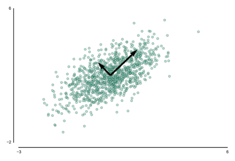
Figure 2.9: The principal components, shown as black arrows, are the orthogonal vectors maximizing the variance of the samples drawn here from a multivariate Gaussian distribution.

Principal component analysis reduces the dimensionality of the dataset by keeping a fraction of the principal components vectors which totalize a large amount of the total variance. If we keep only two components, PCA allows to visualize high dimensional datasets as illustrated in Figure 2.10 with digits.

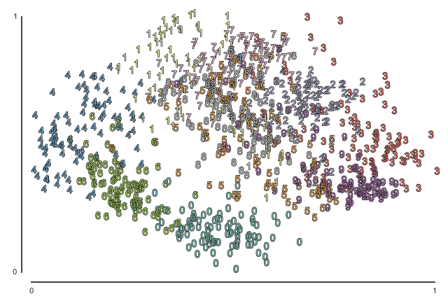
Figure 2.10: We project the digits dataset Lichman (2013) from its $8~\times 8$ pixel space on the two principal components with the largest variance ($29\%$ of the total variance). Digits such as $4$ or $0$ form well defined clusters on this two dimensional space.

Mathematically, we want to find the first principal component vector $u^{1}$ which maximizes the variance along its direction:

$$u^{1}= \arg\max_{u}\sum_{i=1}^{n}||u^{T}x^{i}-u^{T}\sum_{l=1}^{n}\frac{x^{l}}{n}||^{2}_{\ell_{2}}$$

s.t. $$u^{T}u=1.$$ (2.80)

Given that the covariance matrix $C$ is given by

$$C=\sum_{i=1}(x^{i}-\sum_{l=1}^{n}\frac{x^{l}}{n})(x^{i}-\sum_{l=1}^{n}\frac{x^{l}}{n})^{T},$$

we have

$$u^{1}=\arg\max_{u}u^{T}Cu+\lambda_{1}(1-u^{T}u),$$ (2.81)

where $\lambda_{1}$ is the Lagrange multiplier of the normalization constraint.

By derivating with respect to $u$ and setting the first derivative to zero, we have that the maximum is indeed an eigen vector of the covariance matrix:

$$Cu^{1}=\lambda_{1}u^{1}$$ (2.82)

We also note that the variance along $u^{1}$ is given by ${u^{1}}^{T}Cu^{1}=\lambda_{1}$. Thus $u^{1}$ is the eigenvector with the highest eigen value.

The following vector $u^{m+1}$ maximizing the variance are obtained by imposing that the $m+1$-th vector is orthogonal to the $m$ previous one:

$$u^{m+1}=\arg\max_{u^{m+1}}{u^{m+1}}^{T}Cu^{m+1}$$

s.t. $${u^{m+1}}^{T}u^{m+1}=1,$$

$${u^{m+1}}^{T}u^{l}=0\quad\forall l\in~\{1,\ldots,m\},$$ (2.83)

or alternatively in Lagrangian form

$$\arg\max_{u^{m+1}}{u^{m+1}}^{T}Cu^{m+1}+\lambda_{m+1}(1-{u^{m+1}}^{T}u^{m+1})+\sum_{l=1}^{m}\mu_{l}{u^{m+1}}^{T}u^{l}.$$ (2.84)

By differentiating with respect to $u^{l}$ and multiplying by $u^{m+1}$, we have that the Lagrangian constants of the orthogonality constraints are equal to zero $\mu_{l}=0~\,\forall l\in~\{1,\ldots,m\}$. And it follows that the $m+1$-th principal component is the $m+1$-th eigen vector with the $m+1$-th largest eigen value $\lambda_{m+1}$ since

$$Cu^{m+1}=\lambda_{m+1}u^{m+1},{u^{m+1}}^{T}Cu^{m+1}=\lambda_{m+1}.$$ (2.85)

8.2   Random projection

Random projection is a dimensionality reduction method which projects the space onto a smaller random space. For randomly projection, the Jonhson-Lindenstrauss lemma gives the conditions of existence such that the distance between pairs of points is approximately preserved.

Remark 8.4.

Johnson-Lindenstrauss lemma Johnson and Lindenstrauss (1984) Given $\epsilon>0$ and an integer $n$, let $q$ be a positive integer such that $q\geq 8\epsilon^{-2}\ln{n}$. For any sample $(y^{i})_{i=1}^{n}$ of $n$ points in $\mathbb{R}^{d}$ there exists a matrix $\Phi\in\mathbb{R}^{q\times d}$ such that for all $i,j\in\{1,\ldots,n\}$

$$(1-\epsilon)||y^{i}-y^{j}||^{2}\leq||\Phi y^{i}-\Phi y^{j}||^{2}\leq(1+\epsilon)||y^{i}-y^{j}||^{2}.$$ (2.86)

Moreover, when $d$ is sufficiently large, several random matrices satisfy Equation 2.86 with high probability. In particular, we can consider Gaussian matrices whose elements are drawn i.i.d. in $\mathcal{N}(0,1/q)$, as well as (sparse) Rademacher matrices whose elements are drawn in the finite set $\left\{-\sqrt{\frac{s}{q}},0,\sqrt{\frac{s}{q}}\right\}$ with probability $\left\{\frac{1}{2s},1-\frac{1}{s},\frac{1}{2s}\right\}$, where $1/s\in(0,1]$ controls the sparsity of $\Phi$. If $s=3$, we will say that those projections are Achlioptas random projections Achlioptas (2003). When the size of the original space is $p$ and $s=\sqrt{p}$, then we will say that we have sparse random projection as in Li et al. (2006). Note a random sub-space Ho (1998) is also a random projection scheme Candes and Plan (2011): the projection matrix $\Phi$ is obtained by sub-sampling with or without replacement the identity matrix. Theoretical results proving 2.86 with high probability for each random projection matrix can be found in the relevant paper.

The choice of the number of random projections $q$ is a trade-off between the quality of the approximation and the size of the resulting embedding as illustrated in Figure 2.11.

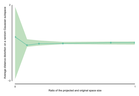
Figure 2.11: Given a set of samples $(x^{i})_{i=0}^{2000}\in\mathbb{R}^{500}$ drawn from a Gaussian distribution, a few random projections preserve on average the distance between pairs of points up to a distortion $\epsilon$.

8.3   Kernel functions

A kernel function $k:\mathcal{X}\times\mathcal{X}\rightarrow\mathbb{R}$ computes the similarity between pairs of samples (usually in the input space). Machine learning algorithms relying solely on dot products, such as support vector machine Cortes and Vapnik (1995) or principal components analysis Jolliffe (2002), are indeed using the linear kernel $k(x^{i},x^{j})={x^{i}}^{T}x^{j}$. We can kernelize these algorithms by replacing their dot product with a kernel presented in Table 2.5. This is the so called kernel trick Scholkopf and Smola (2001). Kernel functions define non linear projection schemes lifting the original space to the one defined by the chosen kernel. It has been used in classification Hsu et al. (2003), in regression Jaakkola and Haussler (1999) and in clustering Schölkopf et al. (1997). Random kernels Rahimi and Recht (2007, 2009) can be used to compress the input space.

Table 2.5: Some common kernel functions between two vectors $x^{i}$ and $x^{j}$.

Kernels
Linear kernel	$k(x^{i},x^{j})={x^{i}}^{T}x^{j}$
Polynomial	$k(x^{i},x^{j})=({x^{i}}^{T}x^{j}+r)^{d}$
Gaussian radial basis function	$k(x^{i},x^{j})=\exp(-\gamma||x^{i}-x^{j}||^{2}_{2})$
Hyperbolic tangent	$k(x^{i},x^{j})=\tanh(\kappa{x^{i}}^{T}x^{j}+r)$

The task shown in Figure 2.12b requires to classify points belonging to one of two interleaved moons. Given the non linearities, we can not linearly separate both classes as illustrated in Figure 2.12b with a (linear) support vector machine. By lifting the linear kernel to the radial basis function kernel, the support vector machine algorithm now separates both classes as shown in Figure 2.12c. Effectively, kernel functions enable machine learning algorithms to handle a wide varieties of structured and unstructured data such as sequences, graphs, texts or vectors through an appropriate choice and design of kernel functions.

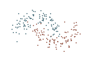
(a) Classification task

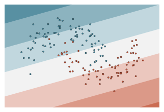
(b) Linear SVM

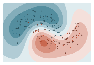
(c) Radial basis function SVM

Figure 2.12: The classification task consists in discriminating points belonging to one of the two interleaved moons (the blue or the red dots). Given the non linearities of the data, a linear support vector machine is not able to find a hyperplane separating both classes as shown in Figure 2.12b. By lifting the original input space through the radial basis function kernel, we are now able to separate both classes as illustrated in Figure 2.12c retrieving the interleaved moons.

Decision trees

Remark 8.5.

Outline Decision trees are non parametric supervised learning models mapping the input space to the output space. The model is a hierarchical structure made of test and leaf nodes. Starting at the root node, the top of the tree, the test nodes lead the reasoning through the tree structure until reaching a leaf node outputting a prediction. In this chapter, we first describe the decision tree model and show how to predict unseen samples. Then, we present the methods and the techniques to grow and to prune these tree structures. We also introduce how to interpret a decision tree model to gain insights on the studied systems and phenomena.

A decision tree is comparable to a human reasoning organized through a hierarchical set of yes/no questions. As in medical diagnosis, an expert (here the doctor) diagnoses the patient state (“Is the patient healthy or sick?”) by screening the patient body and by retrieving important past patient history through a directed set of questions. We can view each step of the reasoning as a branch of a decision tree structure. Each answer leads either to another question refining a set of hypotheses or finally to a conclusion, a prediction.

The binary questions at test nodes can target binary variables, like “Do you smoke?”, categorical variables, like “Do you prefer pear or apple to orange or lemon?”, or numerical variables, like “Is the outside temperature below 25 degree Celsius (77 degree Fahrenheit)?”. Note that we can formulate multi-way questions as a set of binary questions. For instance, the multi-way question “Do you want to eat a pear, a peach or an apple?” is equivalent to ask sequentially “Do you want to eat a pear or one fruit among peach and apple?”, then you would also ask “Do you want to eat a peach or an apple?” if you answered “a peach or an apple”.

With only numerical input variables, questions that are typically asked are in the form “Is the value of variable $x$ lower than a given value?”. The decision tree is then a geometric structure partionning the input space into a recursive set of $p$-dimensional (hyper)rectangles (also called $p$-orthotopes). The root node first divides the whole input space into two half-spaces. Each of those may further be divided into smaller (hyper)rectangles. The partition structure highlights the hierarchical nature of a decision tree. An artistic example of such partitioning in a two dimensional space is the “Composition II in Red, Blue, and Yellow” by Piet Mondrian shown in Figure 3.1. Here, Piet Mondrian divides hierarchically the whole painting into colored rectangles through heavy thick black lines. Each black line is conceptually a testing node of a decision tree, while the colored rectangles would be the predictions of leaves node.

Figure 3.1: Reproduction of “Composition II in Red, Blue, and Yellow” of Piet Mondrian.

Decision trees are popular machine learning model, because of several nice properties:

• The hierarchical nature of the model takes into account non linear effects between the inputs and outputs, as well as conditional dependencies among inputs and outputs.

• Growing a decision tree is computationally fast.

• Decision tree techniques work with heterogeneous data combining binary, categorical or numerical input variables.

• Decision trees are interpretable models giving insights on the relationship between the inputs and the outputs.

• The tree training algorithm can be adapted to handle missing input values Friedman (1977); Breiman et al. (1984); Quinlan (1989).

In Section 9, we present the structure of such models and how to exploit these to predict unseen samples. We show in Section 10 how to train a decision tree model. In Section 11, we describe the techniques used to prune a fully grown decision tree to the right size: too shallow trees tend to under-fit the data as they might lack predicting power, while large trees might overfit the data as they are too complex. In Section 12, we show how to interpret a decision tree to gain insights over the input-output relationships: (i) through input variable importance measures and (ii) through the conversion of the tree structure to a set of rules. In Section 13, we show how to extend decision trees to handle multi-output tasks.

9   Decision tree model

The binary decision tree model is a tree structure built by recursively partitioning the input space. The root node is the node at the top of the tree. We distinguish two types of nodes: (i) the test nodes, also called internal nodes or branching nodes, and (ii) the leaves outputting predictions, also called external nodes or terminal nodes. A test node $N_{t}$ has two children called the left child and the right child; it furthermore has a splitting rule $s_{t}$ testing whether or not a sample belongs to its left or right child. For a continuous or categorical ordered input, the splitting rules are typically of the form $s_{t}(x)=x_{F_{t}}\leq\tau_{t}$ testing whether or not the input value $x_{F_{t}}$ is smaller or equal to a constant $\tau_{t}$. For a binary or categorical input, the splitting rule is of the form $s_{t}(x)=x_{F_{t}}\in B_{t}$ testing whether or not the input value $x_{F_{t}}$ belongs to the subset of values $B_{t}$.

The decision tree of Figure 3.2 first splits the input space into two disjoint partitions $A_{2}=\{x:x_{F_{1}}\leq\tau_{1}\}$ and $A_{3}=\{x:x_{F_{2}}>\tau_{1}\}$ at the root node $N_{1}$. The node $N_{1}$ has two children: $N_{2}$ the left child and $N_{3}$ the right child. The node $N_{2}$ is a leaf and thus a terminal partition. The test node $N_{3}$ further splits the input space based on a categorical set $B_{3}$ into partitions $A_{4}=\{x~\in A_{3},x_{F_{3}}\in B_{3}\}$ and $A_{5}=\{x~\in A_{3},x_{F_{3}}\in B_{3}\}$ with $A_{3}=A_{4}\cup A_{5}$. The input space is further split with 3 more testing nodes with two continuous splitting rules ($N_{4}$, $N_{5}$) or one categorical splitting rule $N_{8}$. The remaining nodes $N_{6}$, $N_{7}$, $N_{9}$, $N_{10}$ and $N_{11}$ are leaf nodes. In total, the decision tree defines a partition of the input space into 11 (hyper)rectangles ($A_{1},\ldots,A_{11}$). A one to one relationship exists between the leaf nodes and the subsets of this input space partition. Note that all partitions of the input space are not expressible as a decision tree structure.

Figure 3.2: A binary decision tree structure containing 11 nodes: 5 test nodes and 6 leaves nodes.

A decision tree predicts the output of an unseen sample by following the tree structure as described by Algorithm 1. The recursive process starts at the root node, then the splitting rules of the testing nodes send the sample further down the tree structure. We traverse the tree structure until reaching a leaf, a terminal node, outputting its associated prediction value. A decision tree model $\hat{f}:\mathcal{X}\rightarrow\mathcal{Y}$ is then expressible as a sum of indicator functions, denoted by $1$, over the $|T|$ tree nodes:

$$\hat{f}(x)=\sum_{t=1}^{|T|}\beta_{t}1(x\in A_{t})1(t\text{ is a leaf})$$ (3.1)

where $\beta_{t}$ is the prediction associated to a node $N_{t}$. The computational complexity of predicting an unseen sample is thus proportional to the depth of the followed branch.

Algorithm 1 Predict a sample $x$ with a decision tree.

1:function tree_predict($tree$, $x$)

2:     $t\leftarrow$ Index of the root node of the tree.

3:     while the node $N_{t}$ is not a leaf. do

4:         if The splitting rule $s_{t}(x)$ of node $N_{t}$ is true then

5:              $t\leftarrow$ Index of the left child of node $N_{t}$.

6:         else

7:              $t\leftarrow$ Index of the right child node $N_{t}$.

8:         end if

9:     end while

10:     return $\beta_{t}$.

11:end function

Remark 9.6.

Binary versus multi-way partitions Decision trees do not have to respect a binary tree structure. Each one of their internal nodes could have more than two children with multi-way splitting rules. However such multi-way partitions are equivalent to a set of consecutive binary partitions. Furthermore, multi-way splits tends to quickly fragment the training data during the decision tree growth impeding its generalization performance. In practice, decision trees are therefore most of the time restricted to be binary. Hastie et al. (2009)

10   Growing decision trees

We grow a decision tree using a set of samples of input-output pairs. Tree growth starts at the root node and divides recursively the input space through splitting rules until we reach a stopping criterion such as a maximal tree depth or minimum sample size in a node. For each new testing node, we search for the best splitting rule to divide the sample set at that node into two subsets. We hope to make partitions “purer” at each new division. The decision tree growing procedure has three main elements:

• a splitting rule search algorithm (see Section 10.1);

• stop splitting criteria (see Section 10.3) which dictate whenever we stop the development of a branch;

• a leaf labelling rule (see Section 10.2) determining the output value of a terminal partition.

Putting all those key elements together leads to the decision tree growing algorithm shown in Algorithm 2.

Algorithm 2 Grow a decision tree using the sample set $\mathcal{L}=\{(x^{i},y^{i})\in\mathcal{X}\times\mathcal{Y}\}_{i=1}^{n}$.

1:function grow_tree($\mathcal{L}$)

2:     $q=$EmptyQueue()

3:     Initialize the tree structure with the root node ($N_{1}$)

4:     $q$.enqueue($(1,\mathcal{L})$).

5:     while $q$ is not empty  do

6:         $(t,\mathcal{L}_{t})\leftarrow q$.dequeue( )

7:         if Node $N_{t}$ satisfies one stopping criterion then

8:              Label node $t$ as a leaf using samples $\mathcal{L}_{t}$

9:         else

10:              Search for the best splitting rule $s_{t}$ using samples $\mathcal{L}_{t}$.

11:              Split $\mathcal{L}_{t}$ into $\mathcal{L}_{t,r}$ and $\mathcal{L}_{t,l}$ using the splitting rule $s_{t}$.

12:              Label node $t$ as a test node with the splitting rule $s_{t}$.

13:              $q$.enqueue(($2t,\mathcal{L}_{t,l}$)).

14:              $q$.enqueue(($2t+1,\mathcal{L}_{t,r}$)).

15:         end if

16:     end while

17:     return The grown decision $tree$.

18:end function

10.1   Search among node splitting rules

During tree growing, we recursively partition the input space $\mathcal{X}$ and the sample set $\mathcal{L}=\{(x^{i},y^{i})\in\mathcal{X}\times\mathcal{Y}\}_{i=1}^{n}$. At each testing node $t$, we split the sample set $\mathcal{L}_{t}$ reaching node $t$ into two smaller subsets $\mathcal{L}_{t,l}$ and $\mathcal{L}_{t,r}$ using a binary splitting rule $s_{t}:\mathcal{X}\rightarrow\{0,1\}$ as shown in Figure 3.3. This raises two questions (i) what is the set of available binary and axis-wise splitting rules $\Omega(\mathcal{L}_{t})$ given a sample set $\mathcal{L}_{t}$ and (ii) how to select the best one among all of them so as to make the descendants “purer” than the parent node.

Figure 3.3: During tree growing (here for a binary classification task with orange and black classes), we search for the best splitting rule $s_{t}$ to divide the sample set $\mathcal{L}_{t}$ reaching node $t$ into a left $\mathcal{L}_{t,l}$ and a right $\mathcal{L}_{t,r}$ subsets.

For a variable $x_{j}\in\mathcal{X}_{j}$ of cardinality $c_{j}$, the associated family $Q(x_{j})$ of splitting rules consists of all possible subsets of $\mathcal{X}_{j}$:

$$Q(x_{j})=\left\{s_{t}(x)\equiv 1(x_{j}\in\mathcal{X}^{\prime}):\mathcal{X}^{\prime}\subset\mathcal{X}_{j}\right\}.$$ (3.2)

The size of the splitting rule family is increasing exponentially with the total number of possible values ($|Q(x_{j})|=2^{|\mathcal{X}_{j}|-1}$).

If the possible values of the variable $x_{j}$ are also ordered, we can reduce the size of the splitting rule family $Q(x_{j})$ from an exponential number of candidates to a linear number of splitting rules ($|Q(x_{j})|=|\mathcal{X}_{j}|-1$):

$$Q(x_{j})= \Bigg{\{}s_{t}(x)\equiv 1(x_{j}\leq\tau):\tau\in\mathcal{X}_{j}\Bigg{\}}.$$ (3.3)

With a numerical variable $x_{j}\in\mathbb{R}$, the number of possible splitting rules is infinite. However, the training set is of finite size. We consider a family of splitting rules similar to Equation 3.3 with the possible values $\tilde{\mathcal{X}}_{j}$ available in the training set.

The selected splitting rule $s_{t}$ should split the sample set $\mathcal{L}_{t}$ such that the following conditions hold: the sample sets $\mathcal{L}_{t,r}$ and $\mathcal{L}_{t,l}$ are non empty ($\mathcal{L}_{t,r}\not=\emptyset$, $\mathcal{L}_{t,l}\not=\emptyset$) forming a disjoint ($\mathcal{L}_{t,l}\cap\mathcal{L}_{t,r}=\emptyset$) and non overlapping partition ($\mathcal{L}_{t}=\mathcal{L}_{t,l}\cup\mathcal{L}_{t,r}$) of the original sample set $\mathcal{L}_{t}$. During the expansion of a test node $t$ into a left child and a right child, we thus select a splitting rule $s_{t}$ among all possible splitting rules $\Omega(\mathcal{L}_{t})$:

$$s_{t}\in\Omega(\mathcal{L}_{t})= \Bigg{\{}s:s\in\bigcup_{j\in\{1,\ldots,p\}}Q(x_{j}),$$

$$\quad\mathcal{L}_{t,l}=\{(x,y)\in\mathcal{L}_{t}:s(x)=1\},$$

$$\quad\mathcal{L}_{t,r}=\{(x,y)\in\mathcal{L}_{t}:s(x)=0\},$$

$$\quad\mathcal{L}_{t,l}\not=\emptyset,\mathcal{L}_{t,r}\not=\emptyset\Bigg{\}}.$$ (3.4)

We strive to select the “best” possible local splitting rule $s_{t}$ for the split at node $t$ leading ideally to good generalization performance. However, it is impossible to minimize directly the generalization error. Thus instead, we are going to minimize the resubstitution error, the error over the training set. However, obtaining such a tree is trivial and it has poor generalization performance. A more meaningful criterion is to search for the smallest tree minimizing the resubstitution error. However, this optimization problem is a NP-complete Hyafil and Rivest (1976). Instead, we greedily grow the tree by maximizing the reduction of an impurity measure function $I:(\mathcal{X}\times\mathcal{Y})\times\ldots\times(\mathcal{X}\times\mathcal{Y})\rightarrow\mathbb{R}$. Mathematically, we define the impurity reduction $\Delta I$ obtained by dividing the sample set $\mathcal{L}_{t}$ into two partitions $(\mathcal{L}_{t,r},\mathcal{L}_{t,l})$ as

$$\Delta I(\mathcal{L}_{t},\mathcal{L}_{t,l},\mathcal{L}_{t,r})=I(\mathcal{L}_{t})-\frac{|\mathcal{L}_{t,l}|}{|\mathcal{L}_{t}|}I(\mathcal{L}_{t,l})-\frac{|\mathcal{L}_{t,r}|}{|\mathcal{L}_{t}|}I(\mathcal{L}_{t,r}).$$ (3.5)

The splitting rule selection problem (line 10 of the tree growing Algorithm 2) is thus written as

$$s_{t}=\arg\max_{s\in\Omega(\mathcal{L}_{t})}\Delta I(\mathcal{L}_{t},\mathcal{L}_{t,l},\mathcal{L}_{t,r})$$ (3.6)

Intuitively, the impurity $I$ should be minimal whenever all samples have the same output value. The node is then said to be “pure”

Given the additivity of the impurity reduction, the best split at node $t$ according to the impurity reduction computed locally is also the best split at this node in terms of global impurity. The remaining tree impurity $Imp(T)$ of a tree $T$ is the sum of the remaining impurities of all leaf nodes:

$$Imp(T)=\sum_{t\in T}p(t)I(\mathcal{L}_{t})1(t\text{ is a leaf})$$ (3.7)

with $p(t)=|\mathcal{L}_{t}|/|\mathcal{L}|$ the proportion of samples reaching node $t$. If we develop the leaf node $t$ into a test node, it leads to a new tree $T^{\prime}$ with a new splitting rule $s_{t}$ having a left $t_{l}$ and a right $t_{r}$ children node. The overall impurity decreases from the original tree $T$ to the bigger tree $T^{\prime}$ and the impurity decrease is given by

$$Imp(T)-Imp(T^{\prime}) =p(t)I(\mathcal{L}_{t})-p(t_{l})I(\mathcal{L}_{t,l})-p(t_{r})I(\mathcal{L}_{t,r})$$ (3.8)

$$=p(t)\Delta I(\mathcal{L}_{t},\mathcal{L}_{t,l},\mathcal{L}_{t,r})$$ (3.9)

Thus, the decision tree growing procedure is a repeated process aiming at decreasing the total impurity as quickly as possible by suitably choosing the local splitting rules.

In classification, a node is pure if all samples have the same class. Given a sample set $\mathcal{L}_{t}$ reaching node $t$, we will denote by $p(y=l|t)=\frac{1}{|\mathcal{L}_{t}|}\sum_{(x,y)\in\mathcal{L}_{t}}1(y=l)$ the proportion of samples reaching node $t$ having the class $l$. A node will be pure if $p(y=l|t)$ is equal to 1 for a class $l$ and zero for the others. The node impurity should increase whenever samples with different classes are mixed together. We require that the impurity measure $I$ in classification satisfies the following properties:

1. $I$ is minimal only whenever the node is pure $p(y=l|t)=1$ and $p(y=m|t)=0\quad\forall m\in\{1,\ldots,l-1,l+1,\ldots,k\}$;

2. $I$ is maximal only whenever $p(y=l|t)=1/k\quad\forall l\in\{1,\ldots,k\}$;

3. $I$ is a symmetric function with respect to the class proportions $p(y=1|t),\ldots,p(y=k|t)$ so as not to favor any class.

A first function satisfying those three properties is the misclassification error rate:

$$\text{Error rate}(\mathcal{L}_{t})=1-\max_{l\in\{1,\ldots,k\}}p(y=l|t).$$ (3.10)

However, this is not an appropriate criterion. In practice, many candidate splitting rules have often the same error rate reduction, especially in the multi-class classification where only the number of samples of the majority class matters.

Consider the following split selection problem, we have a binary classification task with 500 negative and 500 positive samples. The first splitting rule leads to a left child with 125 positive and 375 negative samples, while the right child has 375 positive and 125 negative samples. The misclassification error reduction is thus given by:

$$\frac{500}{1000}-2\frac{500}{1000}(1-\frac{375}{500})=0.25.$$

Now, let’s consider a second splitting rule leading to a pure node with 250 positive samples and another node with 250 positive and 500 negative samples. This second split has the same impurity reduction score leading to a tie:

$$\frac{500}{1000}-\frac{750}{1000}(1-\frac{500}{750})-\frac{250}{1000}(1-\frac{250}{250})=0.25.$$

The misclassification does not discriminate enough node purity as it varies linearly with the fraction of the majority class. To solve this issue, we add a fourth required properties to classification impurity functions Breiman et al. (1984):

1. $I$ must be a strictly concave function with respect to the class proportion $p(y=l|t)$.

This fourth property will increase the granularity of impurity reduction scores leading fewer ties in splitting rule scores. It will reduce the tree instability with respect to the training set.

Two more suitable classification impurity criteria satisfying all four properties are the Gini index, a statistical dispersion measure, and the entropy measure, an information theory measure.

$$Gini(\mathcal{L}_{t}) =\sum_{l=1}^{k}p(y=l|t)(1-p(y=l|t))$$ (3.11)

$$Entropy(\mathcal{L}_{t}) =-\sum_{l=1}^{k}p(y=l|t)\log{p(y=l|t)}$$ (3.12)

By minimizing the Gini index, we minimize the class dispersion. While selecting the splitting rule based on the entropy measure minimizes the unpredictability of the target, the remaining unexplained information of the output variable.

Given the strict concavity of the Gini index and entropy, we can now discriminate the two splits of the previous example. The first split would have an impurity reduction with the Gini index of $0.0625$ and the entropy of $\approx 0.131$. The second split with a pure node would have an impurity reduction of $\approx 0.083$ with the Gini index and of $\approx 0.216$ with the entropy. Based on these criteria, both measures would choose the second split.

In regression tasks, we consider a node as pure if the dispersion of the output values is zero. We require the impurity regression criterion to be zero only if all output values have the same value. A common dispersion measure used to grow regression trees is the empirical variance

$$Variance(\mathcal{L}_{t})=\frac{1}{|\mathcal{L}_{t}|}\sum_{(x,y)\in\mathcal{L}_{t}}\left(y-\bar{y}\right)^{2},\text{ with }\bar{y}=\frac{1}{|\mathcal{L}_{t}|}\sum_{(x,y)\in\mathcal{L}_{t}}y$$ (3.13)

By maximizing the variance reduction, we are searching for a splitting rule minimizing the square loss $\ell(y,y^{\prime})=\frac{1}{2}(y-y^{\prime})^{2}$. Note that the Gini index and the empirical variance lead to the same impurity measure for binary classification tasks and multi-label classification tasks with output classes encoded with $\{0,1\}$ numerical variables.

10.2   Leaf labelling rules

When tree growing is stopped by the activation of a stop splitting criterion, the newly created leaf needs to be labeled by an output value (see line 8 of Algorithm 2). It is a constant $\beta_{t}$ chosen to minimize a given loss function $\ell$ over the samples $\mathcal{L}_{t}=\{(x,y)\in(\mathcal{X},\mathcal{Y})\}$ reaching the node $t$:

$$\beta_{t}=\arg\min_{\beta}\sum_{(x,y)~\in\mathcal{L}_{t}}\ell(y,\beta).$$ (3.14)

In regression tasks, we want to find the constant $\beta_{t}$ minimizing the square loss in single output regression :

$$\beta_{t}=\arg\min_{\beta}~\sum_{(x,y)\in\mathcal{L}_{t}}\frac{1}{2}(y-\beta_{t})^{2}$$ (3.15)

By setting the first derivative to zero, we have

$$\sum_{(x,y)~\in\mathcal{L}_{t}}(y-\beta)=0$$ (3.16)

$$\beta_{t}=\frac{1}{|\mathcal{L}|_{t}}\sum_{(x,y)~\in\mathcal{L}_{t}}y.$$ (3.17)

The constant leaf model minimizing the square loss is the average output value of the samples reaching node $t$.

In classification tasks, the constant $\beta_{t}$ minimizing the $0-1$ loss ($\ell_{0-1}(y,y^{\prime}))=1(y\not=y^{\prime})$) is the most frequent class. The decision tree can also be a class probability estimator by outputting the proportion $p(l|t)$ of samples of class $l$ reaching node $t$ from the sample set $\mathcal{L}_{t}$.

Remark 10.7.

Beyond constant leaf modeling The leaf labelling rule can go beyond a constant model with supervised learning models such as linear models Quinlan et al. (1992); Wang and Witten (1996); Frank et al. (1998); Landwehr et al. (2005), kernel-based methods Torgo (1997), probabilistic models Kohavi (1996) or even tree-ensemble models Matthew et al. (2015). It increases the modeling power of the decision tree at the expense of computing time and new hyper-parameters.

10.3   Stop splitting criterion

The tree growth at a node $t$ naturally stops if all the samples $\mathcal{L}_{t}$ reaching the node $t$ (i) share the same output value (zero impurity) or (ii) share the same input values (but not necessarily the same output) as in this case we can not find a valid split of the data. In both cases, we can not find a splitting rule to grow the tree further due to a lack of data.

A tree developed in such ways is then said to be fully developed. The question is “Should we stop sooner the tree growth?”. A testing node $t$ splits the data $\mathcal{L}_{t}$ into two partitions $(\mathcal{L}_{t,l},\mathcal{L}_{t,r})$ leading to a left child node $t_{l}$ and a right child node $t_{r}$. If we denote by $\hat{f}_{t}$, $\hat{f}_{t,r}$ and $\hat{f}_{t,l}$ the leaf models that would be assigned to the nodes $t$, $t_{r}$ or $t_{l}$, we have that the resubstition error reduction $\Delta{}Err$ associated to a loss function $\ell$ is given by:

$$\Delta{}Err =\sum_{(x,y)\in\mathcal{L}_{t}}\ell(y,\hat{f}_{t}(x))-\sum_{(x,y)\in\mathcal{L}_{t,r}}\ell(y,\hat{f}_{t,r}(x))$$

$$\quad-\sum_{(x,y)\in\mathcal{L}_{t,l}}\ell(y,\hat{f}_{t,l}(x))$$ (3.18)

$$=\sum_{(x,y)\in\mathcal{L}_{t,r}}\left[\ell(y,\hat{f}_{t}(x))-\ell(y,\hat{f}_{t,r}(x))\right]$$

$$\quad+\sum_{(x,y)\in\mathcal{L}_{t,l}}\left[\ell(y,\hat{f}_{t}(x))-\ell(y,\hat{f}_{t,l}(x))\right]$$ (3.19)

Since we choose $\hat{f}_{t,r}$ and $\hat{f}_{t,l}$ so as to minimize the resubstitution error on their respective training data ($\mathcal{L}_{t,l}$ and $\mathcal{L}_{t,r}$), the resubstitution error never increases through node splitting. With only “natural” splitting rule, decision trees are optimally fitting the training data.

Stop splitting criteria avoid over-fitting by stopping earlier the tree growth. They are either based on (i) structural properties or on (ii) data statistics. Criteria computed on the left and the right children can also discard splitting rules, for example requiring a minimal number of samples in the left and right children to split a node.

Structural-based stop splitting criteria regularize the tree growth by explicitly limiting the tree complexity, by restricting for example:

• branch depths or

• the total number of nodes.

In the second case, the order in which the tree nodes are split starts to matter and can be chosen so as to maximize the total impurity reduction.

Data-based stop splitting criteria stop the tree growth if some statical properties computed on the data used to split the node are below a threshold such as

• the number of samples reaching the node,

• the number of samples reaching the left and right children obtained after splitting,

• the impurity reduction or

• the p-value of a significance test, such as a Chi-square test, testing the independence of the split and the output variable.

11   Right decision tree size

To find the right decision tree size, there are two main families of complexity reduction techniques, also called pruning techniques: (i) pre-pruning techniques stop the tree growth before the tree is fully developed (line 5 of Algorithm 2 and presented in Section 10.3) and (ii) post-pruning techniques remove tree nodes a posteriori setting a trade-off between the tree size and the resusbstitution error. Both approaches lead to smaller decision trees aiming to improve generalization performance and to simplify decision tree interpretation.

Pre-pruning criteria are straightforward tools to control the decision tree size. However, it is unclear which pruning level (or hyper-parameter values) leads to the best generalization performance. Too “strict” stop splitting criteria will grow shallow trees under-fitting the data. While too “loose” stop splitting criteria have the opposite effect, i.e., growing overly complex trees over-fitting the data.

While pre-pruning techniques select the tree complexity a priori, post-pruning techniques select the optimal complexity a posteriori. A naive approach to post-pruning would be to build independently a sequence of decision trees with different complexity by varying the stop splitting criteria, and then to select the one minimizing an approximation of the generalization error such as the error on a hold out sample set. However, this is not computationally efficient as it re-grows each time a (new) decision tree.

Post-pruning techniques first grow a single decision tree $T$ with very loose or no stop splitting criterion. This decision tree clearly overfits the training data. Then, they select a posteriori a subtree $T^{*}\subseteq T$ among all possible subtrees of $T$. The original decision tree is thus pruned by collapsing nodes from the original tree into new leaf nodes. The post-pruning method minimizes a tradeoff between the decision tree error over a sample set $\mathcal{S}$ and a function measuring the decision tree complexity such as the number of nodes:

$$T^{*}(\lambda)=\arg\min_{\check{T}\subset T}\text{Error}(\mathcal{\mathcal{S}}|\check{T})+\lambda\text{Complexity}(\check{T}).$$ (3.20)

The cost complexity pruning method Breiman et al. (1984), also known as the weakest link pruning, implements Equation 3.20 through a complexity coefficient $C_{\alpha}$ measuring a tradeoff between the resubstitution error of a tree $\check{T}$ and its complexity $|\check{T}|$ defined by the number of leaves:

$$C_{\alpha}(\check{T})=\text{resubstitution error}(\mathcal{L}|\check{T})+\alpha|\check{T}|.$$ (3.21)

For each $\alpha$, there exists a unique tree $\check{T}_{\alpha}$ minimizing the cost complexity coefficient $C_{\alpha}$. Large values of $\alpha$ lead to small trees, while conversely small values of $\alpha$ allow bigger sub-trees. For the extreme case $\alpha=0$ (resp. $\alpha=\infty$), we have the original decision tree $T_{0}$ (resp. the subtree containing only the root node). One can show Breiman et al. (1984) that we can sequentially obtain the $\check{T}_{\alpha}$ from the original tree $T$ by removing the node with the smallest increase in resubtitution error. We select the optimal subtree $T^{*}$ among all subtrees $\check{T}_{\alpha}\subseteq T$ by minimizing an approximation of the generalization error using for instance cross-validation methods.

The reduced error pruning method Quinlan (1987), another post pruning technique, splits the learning set into a training set and a pruning set. It grows on the training set a large decision tree. During the pruning phase, it first computes the error reduction of pruning each node and its descendants on the pruning set, then removes greedily the node reducing the most the error. It repeats this two steps procedure until the error on the pruning set starts increasing.

Other post pruning methods have been developed with pruning criteria based on statistical procedures Quinlan (1987, 1993) or on cost complexity criteria based on information theory Quinlan and Rivest (1989); Mehta et al. (1995); Wallace and Patrick (1993). Instead of relying on greedy processes, authors Bohanec and Bratko (1994); Almuallim (1996) have proposed dynamic programming algorithms to find an optimal sub-tree sequence minimizing the resubtistution error with increasing tree complexity at the expense of computational complexity.

12   Decision tree interpretation

A strength of the decision tree model is its interpretability. A closer inspection reveals that we can convert a decision tree model to a set of mutually exclusive classification or regression rules. We get these rules by following the path from each leaf to the root node. We have converted the decision tree shown in Figure 3.4 to three sets of predicting rules, one for each class of iris flower (Versicolor, Virginica and Setosa):

1. “If Petal width $\leq$ 0.7cm, then Setosa”

2. “If Petal width > 0.7cm and Petal width $\leq$ 1.65cm and Petal length $\leq$ 5.25cm, then Versicolor.”

3. “If Petal width > 0.7cm and Petal width $>$ 1.65cm and Sepal length $\leq$ 5.95cm and Sepal length $>$ 5.85cm, then Versicolor.”

4. “If Petal width > 0.7cm and Petal width $\leq$ 1.65cm and Petal length $>$ 5.25cm, then Virginica.”

5. “If Petal width > 0.7cm and Petal width $>$ 1.65cm and Sepal length $\leq$ 5.95cm and Sepal length $\leq$ 5.85, then Virginica.”

6. “If Petal width > 0.7cm and Petal width $>$ 1.65cm and Sepal length $>$ 5.95cm, then Virginica.”

Remark that given the binary hierarchical structure, some rules are redundant and can be further simplified. For instance, we can collapse the constraints “Petal width > 0.7cm and Petal width $>$ 1.65cm” into “Petal width $>$ 1.65cm” for the 6-th rule.

Figure 3.4: A decision tree is an interpretable set of rules organized hierarchically. For instance, we can recognize a Versicolor iris with two sets of rules. Among the four input variables (petal width, petal length, sepal width and sepal length), the decision tree shows that only one input variable is necessary to classify the Setosa iris variety.

The decision tree model also shows which input variables $x_{1},\ldots,x_{p}$ are important to predict the output variable(s) $y$. During the decision tree growth, we select at each node $t$ an axis-wise splitting rules $s_{t}$ minimizing the reduction of an impurity measure $\Delta{}I$ dividing the samples $\mathcal{L}_{t}$ reaching the node into two subsets $(\mathcal{L}_{t,l},\mathcal{L}_{t,r})$. The mean decrease of impurity (MDI) of a variable $x_{j}$ Breiman et al. (1984) sums, over the nodes of a decision tree $T$ where $x_{j}$ is used to split, the total reduction of impurity associated to the split weighted by the probability of reaching that node over the training set $\mathcal{L}$:

$$\text{MDI}(x_{j})=\sum_{\left\{t\in T:x_{j}\text{ is tested by }s_{t}\right\}}\frac{|\mathcal{L}_{t}|}{|\mathcal{L}|}\Delta{}I(\mathcal{L}_{t},\mathcal{L}_{t,l},\mathcal{L}_{t,r}).$$ (3.22)

The mean decrease of impurity scores and ranks the input variables according to their importances during the decision tree growth process as illustrated in Figure 3.5. It takes into account variable correlations, multivariate and non linear effects. As such, decision trees are often used as pre-processing tools to select a fraction of the top most important variables.

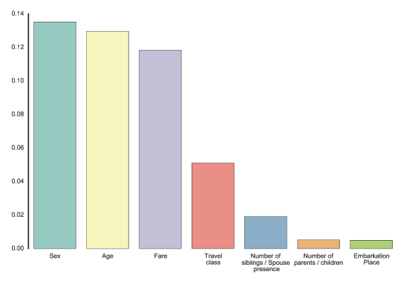
Figure 3.5: Mean impurity decrease for each input variable of the Titanic dataset for a decision tree whose complexity was chosen to maximize the accuracy score on a hold out pruning sample set.

13   Multi-output decision trees

Decision trees naturally extend from single output tasks to multiple output tasks Segal (1992); De’Ath (2002); Blockeel et al. (2000); Clare and King (2001); Zhang (1998); Vens et al. (2008); Noh et al. (2004); Siciliano and Mola (2000) such as multi-output regression, multi-label classification or multi-class classification. No core modification are needed. Instead, we need appropriate impurity measures and leaf labelling rules for the tree prediction Algorithm 1 and the tree growth Algorithm 2. Note that a multi-output decision tree can still be pruned Struyf and Džeroski (2005).

Multi-output impurity measures

During the decision tree growth, we aim to select a splitting rule dividing the sample set $\mathcal{L}_{t}$ reaching the node $t$ into a left and a right sample sets $(\mathcal{L}_{t,l},\mathcal{L}_{t,r})$. The best multi-output splitting rule is the one maximizing the reduction of a multi-output impurity measure $I$. We can use native multi-output impurity measures such as the variance in regression Segal (1992):

$$Variance(\mathcal{L}_{t})=\frac{1}{|\mathcal{L}_{t}|}\sum_{(x,y)\in\mathcal{L}_{t}}\left|y-\bar{y}\right|^{2}_{2}\text{ with }\bar{y}=\frac{1}{|\mathcal{L}_{t}|}\sum_{(x,y)\in\mathcal{L}_{t}}y.$$ (3.23)

or any impurity criterion derived from an appropriate distance measure Blockeel et al. (2000).

We can also extend known impurity measures, such as the Gini index or the entropy (see Section 10.1), by summing the impurity measures over each output De’Ath (2002):

$$I_{mo}(\mathcal{S})=\sum_{j=1}^{d}I(\{(x,y_{j})~\in\mathcal{S}\}),$$ (3.24)

where $S=\{(x^{i},y^{i})\in~(\mathcal{X}\times\mathcal{Y})\}_{i=1}^{n}$ is a sample set.

Since we can define an impurity measure on any set of outputs, we can derive the mean decrease of impurity MDI (see Section 12) either on all or a subset of the outputs.

Leaf labelling and prediction rule

In the multi-output context, the leaf prediction $\beta_{t}$ of a node $t$ is a constant vector of output values chosen so as to minimize a multi-output loss function $\ell$ over the samples $\mathcal{L}_{t}=\{(x^{i},y^{i})\in(\mathcal{X},\mathcal{Y})\}_{i=1}^{n}$ reaching the node:

$$\beta_{t}=\arg\min_{\beta}\sum_{(x,y)~\in\mathcal{L}_{t}}\ell(y,\beta).$$ (3.25)

In multi-output regression, the loss $\ell$ is commonly the $\ell_{2}$-norm loss $\ell_{2}(y,y^{\prime})=\frac{1}{2}||y-y^{\prime}||_{2}^{2}$ the multi-output extension of the square loss. The constant $\beta_{t}$ minimizing the $\ell_{2}$-norm loss is the average output vector

$$\beta_{t}=\frac{1}{|\mathcal{L}_{t}|}\sum_{(x,y)~\in\mathcal{L}_{t}}y.$$ (3.26)

Whenever we extend the label rule assignment to multi-label and to multi-output classification tasks, there are two common possibilities either minimizing the subset $0-1$ loss which is equal to zero if only if all outputs are correctly predicted $\ell_{\text{subset }0-1}(y,y^{\prime})=1(y\not=y^{\prime})$ and the Hamming loss which counts among the $d$ outputs the number of wrongly predicted outputs $\ell_{\text{Hamming}}(y,y^{\prime})=\sum_{j=1}^{d}1(y_{j}\not=y^{\prime}_{j})$.

Minimizing the subset $0-1$ loss takes into account output correlations. The constant vector $\beta_{t}$ minimizing this loss is the most frequent output value combination. Note that the constant $\beta_{t}$ might not be unique as we might have several output combinations with the same frequency of appearance in the sample set reaching the leaf.

The Hamming loss makes the assumption that all outputs are independent. The constant $\beta_{t}$ minimizing this loss is the vector containing the most frequent class of each output.

When the trees are fully developed with only pure leaves, minimizing the Hamming loss or the subset $0-1$ loss leads to identical leaf prediction rules.

Bias-variance and ensemble methods

Remark 13.8.

Outline Ensemble methods combine supervised learning models together so as to improve generalization performance. We present two families of ensemble methods: averaging methods and boosting methods. Averaging ensembles grow independent unstable estimators and average their predictions. Boosting methods increase sequentially their total complexity by adding biased and stable estimators. In this chapter, we first show how to decompose the generalization error of supervised learning estimators into their bias, variance and irreducible error components. Then we show how to exploit averaging techniques to reduce variance and boosting techniques to sequentially decrease bias.

Ensemble methods fit several supervised learning models instead of a single one and combine their predictions. The goal is to reduce the generalization error by solving the same supervised learning task multiple times. We hope that the errors made by the different models will compensate and thereby improve the overall accuracy whenever we consider them together.

Real life examples of “ensemble methods” in the human society are democratic elections. Each eligible person is asked to cast its vote for instance to choose between political candidates. This approach considers each person of the committee as an independent expert and averages simultaneously their opinions. In supervised learning, these kinds of voting mechanism are called “averaging methods”.

Instead of querying all experts independently, we can instead collect their opinions sequentially. We ask to each new expert to refine the predictions made by the previous ones. The expert sequence is chosen so that each element of the sequence improves the accuracy focusing on the unexplained phenomena. For instance in medical diagnosis, a person itself is the first one to assess its health status. The next expert in the line is the general practitioner followed by a series of specialists. We call these ensemble methods “boosting methods”.

The “averaging” approach aims to reduce the variability in the expert pool by averaging their predictions. At the other end, the “boosting” approach carefully refines its predictions by cumulating the predictions of each expert.

In Section 14, we show how to decompose the error made by supervised learning models into three terms: a variance term due to the variability of the model with respect the learning sample set, a bias term due to a lack of modeling power of the estimator and an irreducible error term due to the nature of the supervised learning task. Averaging methods presented in Section 15 are variance reducing techniques growing independently supervised learning estimators. In Section 16, we show how to learn sequentially a series of estimators through boosting methods increasing the overall ensemble complexity and reducing the ensemble model bias.

14   Bias-variance error decomposition

The expected error or generalization error $Err$ associated to a loss $\ell:\mathcal{Y}\times\mathcal{Y}\rightarrow\mathbb{R}^{+}$ of a supervised learning algorithm is a random variable depending on the learning samples $\mathcal{L}=\{(x^{i},y^{i})\in\mathcal{X}\times\mathcal{Y}\}_{i=1}^{n}$ drawn independently and identically from a distribution $P_{{\cal X},{\cal Y}}$ and used to fit a model $f_{\mathcal{L}}:\mathcal{X}\rightarrow\mathcal{Y}$ in a hypothesis space $\mathcal{H}\subset\mathcal{Y}^{\mathcal{X}}$. We want here to analyze the expectation of the generalization error $Err$ over the distribution of learning samples defined as follows:

$$\operatorname{E}_{\mathcal{L}}(Err) =\operatorname{E}_{\mathcal{L}}\operatorname{E}_{P_{\mathcal{X},\mathcal{Y}}}\left\{\ell(f_{\mathcal{L}}(x),y)\right\}$$ (4.1)

$$=\operatorname{E}_{\mathcal{L}}\operatorname{E}_{P_{\mathcal{X}}}\operatorname{E}_{P_{\mathcal{Y}|\mathcal{X}}}\left\{\ell(f_{\mathcal{L}}(x),y)\right\}$$ (4.2)

Let us denote the Bayes model by $f_{\text{Bayes}}(x)\in\mathcal{Y}^{\mathcal{X}}$, the best model possible minimizing the generalization error:

$$f_{\text{Bayes}}(x)=\arg\min_{f\in\mathcal{Y}^{\mathcal{X}}}\operatorname{E}_{P_{\mathcal{X},\mathcal{Y}}}\left\{\ell(f(x),y)\right\}.$$ (4.3)

For the squared loss $\ell(y,y^{\prime})=\frac{1}{2}(y-y^{\prime})^{2}$, we can decompose the expected error over the learning set $\operatorname{E}_{\mathcal{L}}(Err)$ into three terms (see Geman et al. (1992) for the proof):

$$\operatorname{E}_{\mathcal{L}}(Err) \triangleq\operatorname{E}_{\mathcal{L}}\operatorname{E}_{P_{\mathcal{X},\mathcal{Y}}}\left\{(f_{\mathcal{L}}(x)-y)^{2}\right\}$$ (4.4)

$$=\operatorname{E}_{P_{\mathcal{X}}}\left\{\operatorname{Var}_{\mathcal{L}}\left\{f_{\mathcal{L}}(x)\right\}+\operatorname{Bias}^{2}(f_{\mathcal{L}}(x))+\operatorname{Var}_{P_{\mathcal{Y}|\mathcal{X}}}\left\{y\right\}\right\},$$ (4.5)

where

$$\operatorname{Var}_{\mathcal{L}}\left\{f_{\mathcal{L}}(x)\right\} =\operatorname{E}_{\mathcal{L}}\left\{\left(f_{\mathcal{L}}(x)-f_{\text{avg}}(x)\right)^{2}\right\},$$ (4.6)

$$\operatorname{Bias}^{2}(f_{\mathcal{L}}(x)) =\left(\operatorname{E}_{\mathcal{L}}\left\{f_{\mathcal{L}}(x)\right\}(x)-f_{\text{Bayes}}(x)\right)^{2}.$$ (4.7)

We interpret each term of Equation 4.5 as follows:

• The variance of a supervised learning algorithm $\operatorname{E}_{P_{\mathcal{X}}}\operatorname{Var}_{\mathcal{L}}\left\{f_{\mathcal{L}}(x)\right\}$ describes the variability of the model with a randomly drawn learning sample set $\mathcal{L}$. Supervised learning algorithms with a high variance have often a high complexity which makes them overfit the data.

• The square bias $\operatorname{E}_{P_{\mathcal{X}}}\left\{\operatorname{Bias}^{2}(f_{\mathcal{L}}(x))\right\}$ is the distance between the average model and the Bayes model. Biased models are not complex enough to model the input-output function. They are indeed underfitting the data.

• The irreducible error $\operatorname{E}_{P_{\mathcal{X}}}\operatorname{Var}_{P_{\mathcal{Y}|\mathcal{X}}}\left\{y\right\}$ is the variance of the target around its true mean. It is the minimal attainable error on a supervised learning problem.

The bias-variance decomposition allows to analyze and to interpret the effect of hyper-parameters. It highlights and gives insights on their effects on the bias and the variance. In Figure 4.1, we have fitted decision tree models with an increasing number of leaves on the Friedman1 dataset Friedman (1991), a simulated regression dataset. We first assess the resubstitution error over 300 samples and an approximation of the generalization error, the hold out error, computed on an independent testing set of 20000 samples. We compute these errors (see Figure 4.1a) by averaging the performance of decision tree models over 100 learning sets $\mathcal{L}$ drawn from the same distribution $P_{\mathcal{X},\mathcal{Y}}$. By increasing the number of leaves, the resubstitution error decreases up to zero with fully developed trees. On the other hand, the hold out error starts increasing beyond 20 leaves indicating that the model is under-fitting with less than 20 leaves and over-fitting with more than 20 leaves. By increasing the number of leaves, we decrease the bias as we grow more complex models as shown in Figure 4.1b. It also increases the variance as the tree structures become more unstable with the learning set $\mathcal{L}$ .

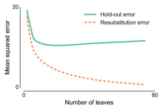
(a)

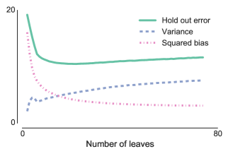
(b)

Figure 4.1: Bias-variance decomposition of decision tree models of increasing complexity on the Friedman1 dataset.

In general, we have the following trends for a single decision tree model. Large decision trees overfit and are unstable with respect to the learning set $\mathcal{L}$ which corresponds to a high variance and a small bias. Shallow decision trees, on the other hand, underfit the learning set $\mathcal{L}$ and have stable structures, which corresponds to a small variance and a high bias. The pruning technique presented in Section 11 allows to select a tradeoff between the variance and the bias of the algorithm by adjusting the tree complexity.

The bias-variance decomposition of the square loss is by far the most studied decomposition, but there nevertheless exist similar decompositions for other losses, e.g. see Domingos (2000) for a decomposition of the polynomial loss $\ell(y,y^{\prime})=|y-y^{\prime}|^{p}$, see Friedman (1997); Kohavi et al. (1996); Tibshirani (1996a); Domingos (2000) for the $0-1$ loss, or see James (2003) for losses in general.

15   Averaging ensembles

An averaging ensemble model $f_{\theta_{1},\ldots,\theta_{M}}$ builds a set of $M$ supervised learning models $\{f_{\theta_{m}}\}_{\theta_{m}=1}^{M}$, instead of a single one. Each model $f_{\theta_{m}}$ of the ensemble is different as we randomize and perturb the original supervised learning algorithm at fitting time. We describe entirely the induced randomization of one model $f_{\theta_{m}}$ by drawing i.i.d. a random vector of parameters $\theta_{m}$ from a distribution of model parameters $P_{\theta}$.

In regression, the averaging ensemble predicts an unseen sample by averaging the predictions of each model of the ensemble:

$$f_{\theta_{1},\ldots,\theta_{M}}(x)=\sum_{m=1}^{M}f_{\theta_{m}}(x).$$ (4.8)

It minimizes the square loss (or its extension the $\ell_{2}$-norm loss) between the ensemble model and its members:

$$f_{\theta_{1},\ldots,\theta_{M}}(x)=\arg\min_{y\in\mathcal{Y}}\sum_{m=1}^{M}(y-f_{\theta_{m}}(x))^{2}.$$ (4.9)

In classification, the averaging ensemble combines the predictions of its members to minimize the 0-1 loss by a majority vote of all its members:

$$f_{\theta_{1},\ldots,\theta_{M}}(x)=\arg\min_{c\in\mathcal{Y}}\sum_{m=1}^{M}1(f_{\theta_{m}}(x)\neq c).$$ (4.10)

An alternative approach, called soft voting, is to classify according to the average of the probability estimates $\hat{P}_{f_{\theta_{m}}(x)}$ provided by the ensemble members:

$$f_{\theta_{1},\ldots,\theta_{M}}(x)=\arg\max_{c~\in\mathcal{Y}}\sum_{m=1}^{M}\hat{P}_{f_{\theta_{m}}(x)}(Y=c).$$ (4.11)

Both approaches have been studied and yield almost exactly the same result, but soft voting provides smoother probability class estimates than majority vote Breiman (1996a); Zhou (2012). The multi-output extension to ensemble predictions often minimizes the Hamming loss applying either soft-voting or majority voting to each output independently. Minimizing the subset $0-1$ loss for multi-label tasks would lead to predict the most frequent label set.

Remark 15.9.

Ambiguity decomposition The ambiguity decomposition Krogh et al. (1995) of the square loss shows that the generalization error of an ensemble $f_{\theta_{1},\ldots,\theta_{M}}$ of $M$ models $\{f_{\theta_{m}}\}_{m=1}^{M}$ is always lower or equal than the average generalization error $\bar{E}$ of its members:

$$\operatorname{E}_{P_{\mathcal{X}}}\operatorname{E}_{P_{\mathcal{Y}|\mathcal{X}}}\left\{(y-f_{\theta_{1},\ldots,\theta_{M}}(x))^{2}\right\}=\bar{E}-\bar{A}\leq\bar{E}$$ (4.12)

with

$$\bar{E} =\frac{1}{M}\sum_{m=1}^{M}\operatorname{E}_{P_{\mathcal{X}}}\operatorname{E}_{P_{\mathcal{Y}|\mathcal{X}}}\left\{(y-f_{\theta_{m}}(x))^{2}\right\}$$ (4.13)

$$\bar{A} =\frac{1}{M}\sum_{m=1}^{M}\operatorname{E}_{P_{\mathcal{X}}}\left\{(f_{\theta_{m}}(x)-f_{\theta_{1},\ldots,\theta_{M}}(x))^{2}\right\}$$ (4.14)

The ambiguity term $\bar{A}$ is the variance of the ensemble around its average model $f_{\theta_{1},\ldots,\theta_{M}}$. The equality occurs only if all average models are identical $f_{\theta_{1},\ldots,\theta_{M}}=f_{\theta_{m}}\quad\forall m\in\{1,\ldots,M\}$.

Averaging ensemble models are obtained by first perturbing supervised learning models and then combining them. They aim to reduce the generalization error of the ensemble compared to the original single model by reducing the variance of the learning algorithm. Let us illustrate the effects of an averaging method called bagging on the bias and variance of fully grown decision trees. The bagging method fits each estimator of the ensemble on a bootstrap copy of the learning set. In Figure 4.2, we show the variance and the bias as function of the number of fully grown decision trees in the bagging ensemble. With a single decision tree, the variance is the dominating error component. By increasing the size of the Bagging ensemble, the variance and the hold out error are reduced, while leaving the bias mostly unchanged.

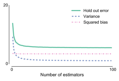
Figure 4.2: Bias-variance decomposition of an ensemble of randomized and fully developed decision tree models fitted on bootstrap copies of the learning set (bagging method) for increasing ensemble size on the Friedman1 dataset. The hold out error, variance and squared bias are averaged over 100 independent learning and testing sets of respective size 300 and 20000 samples.

In Section 15.1, we show how the bias-variance decomposition of a randomized supervised learning algorithm is affected by the ensemble averaging method. In Section 15.2, we present how to induce randomization without modifying the original supervised learning algorithm. In Section 15.3, we describe specific randomization schemes for decision tree methods leading to random forest models.

15.1   Variance reduction

Let us first study the bias-variance decomposition for a model $f_{\mathcal{L},\theta}$ trained on a learning set $\mathcal{L}$ whose randomness is entirely captured by a random vector of parameters $\theta$. The model $f_{\mathcal{L},\theta}$ is thus a function of two random variables $\theta$ and the learning set $\mathcal{L}$. It admits the following bias-variance decomposition of the generalization error for the average square loss Geurts (2002):

$$\operatorname{E}_{\mathcal{L},\theta}(Err)=\operatorname{E}_{P_{\mathcal{X}}}\left\{\operatorname{Var}_{\mathcal{L},\theta}\left\{f_{\mathcal{L},\theta}(x)\right\}+\text{Bias}^{2}(f_{\mathcal{L},\theta}(x))+\operatorname{Var}_{P_{\mathcal{Y}|\mathcal{X}}}\left\{y\right\}\right\},$$ (4.15)

where

$$\operatorname{Var}_{\mathcal{L},\theta}\left\{f_{\mathcal{L},\theta}(x)\right\} =\operatorname{E}_{\mathcal{L},\theta}\left\{\left(f_{\mathcal{L},\theta}(x)-\operatorname{E}_{\mathcal{L}}\operatorname{E}_{\theta}\left\{f_{\theta}(x)\right\}\right)^{2}\right\},$$ (4.16)

$$\operatorname{Bias}^{2}(f_{\mathcal{L},\theta}(x)) =\left(\operatorname{E}_{\mathcal{L}}\operatorname{E}_{\theta}\left\{f_{\mathcal{L},\theta}(x)\right\}-f_{\text{Bayes}}(x)\right)^{2}.$$ (4.17)

By comparison to the bias-variance decomposition of an unperturbed model (see Equation 4.15), we have two main differences:

1. The squared bias is now the distance between the Bayes model $f_{\text{Bayes}}$ and the average model $\operatorname{E}_{\mathcal{L}}\operatorname{E}_{\theta}\left\{f_{\mathcal{L},\theta}(x)\right\}$ over both the learning set $\mathcal{L}$ and the randomization parameter $\theta$. Note that the average model of the randomized algorithm is different from the non-randomized model $\operatorname{E}_{\mathcal{L}}\left\{f_{\mathcal{L}}(x)\right\}$. The randomization of the original algorithm might increase the squared bias.

2. The variance $\operatorname{Var}_{\mathcal{L},\theta}\left\{f_{\mathcal{L},\theta}(x)\right\}$ of the algorithm now depends on the two random variables $\mathcal{L}$ and $\theta$. With the law of total variance, we can further decompose the variance term into two terms:

   $$\operatorname{Var}_{\mathcal{L},\theta}\left\{f_{\mathcal{L},\theta}(x)\right\}=\operatorname{Var}_{\mathcal{L}}\left\{\operatorname{E}_{\theta|\mathcal{L}}\left\{f_{\mathcal{L},\theta}(x)\right\}\right\}+\operatorname{E}_{\mathcal{L}}\operatorname{Var}_{\theta|\mathcal{L}}\left\{f_{\mathcal{L},\theta}(x)\right\}$$ (4.18)

   The first term is the variance brought by the learning sets of the average model over all parameter vectors $\theta$. The second term describes the variance brought by the parameter vector $\theta$ averaged over all learning sets $\mathcal{L}$.

Now, we can study the bias-variance decomposition of the generalization error for an ensemble model $f_{\mathcal{L},\theta_{1},\ldots,\theta_{m}}$ whose constituents $\{f_{\mathcal{L},\theta_{m}}\}_{m=1}^{M}$ depend each on the learning set $\mathcal{L}$ and a random parameter vector $\{\theta_{m}\}_{m=1}^{M}$ capturing the randomness of the models. The bias-variance decomposition of the ensemble model $f_{\theta_{1},\ldots,\theta_{m}}$ is given by

$$\operatorname{E}_{\mathcal{L},\theta_{1},\ldots,\theta_{M}}(Err)= \operatorname{E}_{P_{\mathcal{X}}}\operatorname{Var}_{\mathcal{L}}\left\{\operatorname{E}_{\theta_{1},\ldots,\theta_{M}|\mathcal{L}}\left\{f_{\mathcal{L},\theta_{1},\ldots,\theta_{M}}(x)\right\}\right\}$$

$$+\operatorname{E}_{P_{\mathcal{X}}}\operatorname{E}_{\mathcal{L}}\operatorname{Var}_{\theta_{1},\ldots,\theta_{M}|\mathcal{L}}\left\{f_{\mathcal{L},\theta_{1},\ldots,\theta_{M}}(x)\right\}$$

$$+\operatorname{E}_{P_{\mathcal{X}}}\operatorname{Bias}^{2}(f_{\mathcal{L},\theta_{1},\ldots,\theta_{M}}(x))$$

$$+\operatorname{E}_{P_{\mathcal{X}}}\operatorname{Var}_{P_{\mathcal{Y}|\mathcal{X}}}\left\{y\right\}.$$ (4.19)

Let us compare the decomposition for a single random model (Equations 4.15-4.18) to the decomposition for an ensemble of random models (Equation 4.19). We are going to expand the bias-variance decomposition using the ensemble prediction formula $f_{\theta_{1},\ldots,\theta_{m}}(x)=\frac{1}{M}\sum_{m=1}^{M}f_{\theta_{m}}(x)$ (the demonstration follows Geurts (2002)). As previously, the variance $\operatorname{Var}_{P_{\mathcal{Y}|\mathcal{X}}}(y)$ is irreducible as this term does not depend on the supervised learning model.

The average ensemble model of an ensemble of randomized models is equal to the average model of a single model $f_{\mathcal{L},\theta}$ of random parameter vector $\theta$:

$$\operatorname{E}_{\mathcal{L},\theta_{1},\ldots,\theta_{M}}\left\{f_{\mathcal{L},\theta_{1},\ldots,\theta_{M}}(x)\right\} =\frac{1}{M}\sum_{m=1}^{M}\operatorname{E}_{\mathcal{L}}\operatorname{E}_{\theta_{m}}\left\{f_{\mathcal{L},\theta_{m}}(x)\right\},$$ (4.20)

$$=\operatorname{E}_{\mathcal{L}}\operatorname{E}_{\theta}\left\{f_{\mathcal{L},\theta}(x)\right\}.$$ (4.21)

The squared bias of the ensemble is thus unchanged compared to a single randomized model.

Now, let us consider the two variance terms. The first one depends on the variability of the learning set $\mathcal{L}$. With an ensemble of randomized models, it becomes:

$$\operatorname{E}_{P_{\mathcal{X}}}\operatorname{Var}_{\mathcal{L}}\left\{\operatorname{E}_{\theta_{1},\ldots,\theta_{M}|\mathcal{L}}\left\{f_{\mathcal{L},\theta_{1},\ldots,\theta_{M}}(x)\right\}\right\}~$$

$$=\operatorname{E}_{P_{\mathcal{X}}}\operatorname{Var}_{\mathcal{L}}\left\{\frac{1}{M}\sum_{m=1}^{M}\operatorname{E}_{\theta_{m}|\mathcal{L}}\left\{f_{\mathcal{L},\theta_{m}}(x)\right\}\right\},$$ (4.22)

$$=\operatorname{E}_{P_{\mathcal{X}}}\operatorname{Var}_{\mathcal{L}}\left\{\operatorname{E}_{\theta|\mathcal{L}}\left\{f_{\mathcal{L},\theta}(x)\right\}.\right\}.$$ (4.23)

The variance of the ensemble of randomized model with respect to the learning set $\mathcal{L}$ drawn from the input-output pair distribution $P_{\mathcal{X},\mathcal{Y}}$ is not affected by the averaging and is equal to the variance of a single randomized model.

Let us developed the second variance term of the decomposition describing the variance with respect to the set of random parameter vectors $\theta_{1},\ldots,\theta_{M}$:

$$\operatorname{E}_{P_{\mathcal{X}}}\operatorname{E}_{\mathcal{L}}\operatorname{Var}_{\theta_{1},\ldots,\theta_{m}|\mathcal{L}}\left\{f_{\mathcal{L},\theta_{1},\ldots,\theta_{M}}(x)\right\}~$$

$$=\operatorname{E}_{P_{\mathcal{X}}}\operatorname{E}_{\mathcal{L}}\operatorname{Var}_{\theta_{1},\ldots,\theta_{M}|\mathcal{L}}\left\{\frac{1}{M}\sum_{m=1}^{M}f_{\mathcal{L},\theta_{m}}(x)\right\},$$ (4.24)

$$=\frac{1}{M^{2}}\operatorname{E}_{P_{\mathcal{X}}}\operatorname{E}_{\mathcal{L}}\left\{\sum_{m=1}^{M}\operatorname{Var}_{\theta_{1},\ldots,\theta_{M}|\mathcal{L}}\left\{f_{\mathcal{L},\theta_{m}}(x)\right\}\right\},$$ (4.25)

$$=\frac{1}{M^{2}}\operatorname{E}_{P_{\mathcal{X}}}\operatorname{E}_{\mathcal{L}}\left\{\sum_{m=1}^{M}\operatorname{Var}_{\theta_{m}|\mathcal{L}}\left\{f_{\mathcal{L},\theta_{m}}(x)\right\}\right\},$$ (4.26)

$$=\frac{1}{M}\operatorname{E}_{P_{\mathcal{X}}}\operatorname{E}_{\mathcal{L}}\operatorname{Var}_{\theta|\mathcal{L}}\left\{f_{\mathcal{L},\theta}(x)\right\},$$ (4.27)

where we use the following properties: (i) $\operatorname{Var}\{ax\}=a^{2}\operatorname{Var}\{x\}$ where $a$ is a constant, (ii) at a fixed learning set $\mathcal{L}$, the models $f_{\mathcal{L},\theta_{m}}\,\forall m$ are independent, (iii) the variance of a sum of independent random variables is equal to the sum of the variance of each independent random variables ($\operatorname{Var}\left\{\sum_{i=1}^{n}x_{i}\right\}=\sum_{i=1}^{n}\operatorname{Var}\{x_{i}\}$).

Putting all together the bias-variance decomposition of Equation 4.19 becomes Geurts (2002):

$$\operatorname{E}_{\mathcal{L},\theta_{1},\ldots,\theta_{m}}(Err)= \operatorname{E}_{P_{\mathcal{X}}}\operatorname{Var}_{\mathcal{L}}\left\{\operatorname{E}_{\theta|\mathcal{L}}\left\{f_{\mathcal{L},\theta}(x)\right\}\right\}$$

$$+\frac{1}{M}\operatorname{E}_{P_{\mathcal{X}}}\operatorname{E}_{\mathcal{L}}\operatorname{Var}_{\theta|\mathcal{L}}\left\{f_{\mathcal{L},\theta}(x)\right\}$$

$$+\operatorname{E}_{P_{\mathcal{X}}}\left(\operatorname{E}_{\mathcal{L}}\operatorname{E}_{\theta}\left\{f_{\mathcal{L},\theta}(x)\right\}-f_{\text{Bayes}}(x)\right)^{2}$$

$$+\operatorname{E}_{P_{\mathcal{X}}}\operatorname{Var}_{P_{\mathcal{Y}|\mathcal{X}}}\left\{y\right\}.$$ (4.28)

The bias variance decomposition of an ensemble of randomized models $f_{\mathcal{L},\theta_{1},\ldots,\theta_{M}}$ (see Equation 4.28) shows that averaging $M$ models reduces the variance related to the randomization $\theta$ by a factor $1/M$ over a single randomized model $f_{\mathcal{L},\theta}$ (see Equation 4.15) without modifying the other terms. Note that we can not compare the bias variance decomposition of an ensemble of randomized models $f_{\mathcal{L},\theta_{1},\ldots,\theta_{M}}$ to its non randomized counterparts $f_{\mathcal{L}}$(see Equation 4.5). The bias and variance terms are indeed not comparable.

In practice, we first perturb the learning algorithm which increases the variance of the models and then we combine them through averaging. The variance reduction effect is expected to be higher than the added variance at training time. The bias is either unaffected or increased through the randomization induction. Perturbing the algorithm is thus a tradeoff between the reduction in variance and the increase in bias. An ensemble of randomized models $f_{\mathcal{L},\theta_{1},\ldots,\theta_{M}}$ will have better performance than its non perturbed counterparts $f_{\mathcal{L}}$ if the bias increase is compensated by the variance reduction. In Louppe (2014), the authors have shown that the generalization error is reduced if the randomization induction decorrelates the models of the ensemble.

The previous decomposition does not apply to the $0-1$ loss in classification. However, the main conclusions remains valid Breiman (1996a); Domingos (2000); Geurts (2002).

15.2   Generic randomization induction methods

In this section, we first discuss generic randomization methods to perturb a supervised learning algorithm without modifying the original algorithm through (i) the learning sample set $\mathcal{L}=\{(x^{i},y^{i})\in\mathcal{X}\times\mathcal{Y}\}_{i=1}^{n}$ available at fitting time, (ii) the input space $\mathcal{X}$ or (iii) the output space $\mathcal{Y}$. Those three perturbation principles can be either applied separately or together.

We present in succession these three model agnostic randomization principles (perturbing $\mathcal{L}$, $\mathcal{X}$ or $\mathcal{Y}$).

15.2.1   Sampling-based randomization

One of the earliest randomization method, called bagging Breiman (1996a), fits independent models on bootstrap copies of the learning set. A bootstrap copy Efron (1979) is obtained by sampling with replacement $|\mathcal{L}|$ samples from the learning set $\mathcal{L}$. The original motivation was a first theoretical development and empirical experiments showing that bagging reduces the error of an unstable estimator such as a decision tree. Bootstrap sampling totally ignores the class distribution in the original sample set $\mathcal{L}$ and might lead to highly unbalanced bootstraps. A partial solution is to use stratified bootstraps or to bootstrap Chen et al. (2004) separately the minority and majority classes. In the bagging approach only a fraction of the dataset is provided as training set to each estimator, the wagging approach (Bauer and Kohavi, 1999) fits instead each estimator on the entire training set with random weights. Instead of using bootstrap copies of training set, Büchlmann and Yu (2002) proposes to subsample the training set, i.e. to sample without replacement the training set.

To take into account the input space structure, Kuncheva et al. (2007) proposes to generate random input space partition with a random hyperplane. An estimator is then build for each partition. To get an ensemble, Kuncheva et al. (2007) repeats this process multiple times.

15.2.2   Input-based randomization

Input-based randomization techniques are often based on dimensionality reduction techniques. The random subspace method Ho (1998) builds each model on a random subset of the input space $\mathcal{X}$ obtained by sub-sampling inputs without replacement. It was later combined with the bagging method in Panov and Džeroski (2007), by bootstrapping the learning set $\mathcal{L}$ before learning an estimator, and with sub-sampling techniques with/without replacement in Louppe and Geurts (2012) generating random (sample-input) patches of the data. Note that while we reduce the input space size, we can also over-sample the learning set. For instance, Maree et al. (2005) apply a supervised learning algorithm on random sub-windows extracted from an image, which effectively (i) increases the sample size available to train each model; (ii) reduces the input space size, (iii) and takes into account spatial (pixel) correlation in the images.

Since decision tree made their split orthogonally to the input space, authors have proposed to randomize such ensembles by randomly projecting the input space. Rotation forest Rodriguez et al. (2006) is an ensemble method combining bagging with principal component analysis. For each bootstrap copy, it first slices the $p$ input variables into $q$ subsets, then projects each subset of inputs of size $\frac{p}{q}$ on its principal components and finally grows $q$ models (one on each subset). Kuncheva and Rodríguez (2007) further compares three input dimensionality reduction techniques (described in Section 8): (i) the PCA approach of Rodriguez et al. (2006), (ii) Gaussian random projections and (iii) sparse Gaussian random projections. On their benchmark, they find that the PCA-based rotation matrices yield the best results and also that sparse random projections are strictly better than dense random projections. The idea of using dense Rademacher or Gaussian random projections was again re-discovered by Schclar and Rokach (2009). Similarly, Blaser and Fryzlewicz (2015) proposed to make ensembles through random rotation of the input space.

15.2.3   Output-based randomization

Output-based randomization methods directly perturb the output space $\mathcal{Y}$ of each member of the ensemble.

In regression, we can induce randomization to an output variable through the addition of an independent Gaussian noise Breiman (2000). We fit each model of the ensemble on the perturbed output $y^{\prime}=y+\epsilon_{m}$ with $\epsilon_{m}\sim\mathcal{N}(0;\sigma)$.

In classification, we perturb the output of each model of the ensemble by having a non zero probability to randomly switch the class associated to each sample Breiman (2000); Martínez-Muñoz and Suárez (2005); Martínez-Muñoz et al. (2008).

For multi-label tasks and multi-output tasks, supervised learning algorithms, such as random k-label subset (see also Section 4.5) Tsoumakas and Vlahavas (2007), randomizes the ensemble by building each model of the ensemble on a subset of the output space or the label sets present in the learning set.

15.3   Randomized forest model

The decision tree algorithm has a high variance, due to the instability of its structure. Large decision trees, such as fully developed trees, are often very unstable, especially at the bottom of the tree. The selected splitting rules depend on the samples reaching those nodes. Small changes in the learning set might lead to very different tree structures. Authors have proposed randomization schemes to perturb the search and selection of the best splitting rule improving the generalization error through averaging methods.

One of the first propositions to perturb the splitting rule search Dietterich and Kong (1995) was to select randomly at each node one splitting rule among the top $k$ splitting rules with the highest impurity reduction. The variance of the algorithm increases with the number $k$ of splitting rule candidates, leaving the bias unchanged. Later in the context of digit recognition, Amit et al. (1997) randomized the tree growth by restricting the splitting rule search at each node to a random subset of $k$ input variables out of the $p$ available. The original motivation was to drastically reduce the splitting rule search space as the number of input variables is very high in digit recognition tasks. This randomization scheme increases more the variance of the algorithm than the one of Dietterich and Kong, at the expense of increasing the bias. Note the similarity with the random subspace approach Ho (1998) which subsamples the input space prior fitting a new estimator in an averaging ensemble.

Breiman got inspired by the work of Amit et al. and combined its bagging method Breiman (1996a) with the input variable sub-sampling leading to the well known “random forest” algorithm Breiman (2001). The combination of both randomization schemes has led to one of the best of the shelf estimator for many supervised learning tasks Caruana et al. (2008); Fernández-Delgado et al. (2014).

Later on, Geurts et al. (2006a) randomized the cut point and input variable selection of the splitting rules. At each test node, it draws one random splitting rule for $k$ randomly selected input variables (without replacement) and then selects the best one. This randomized tree ensemble is called extremely randomized trees or extra trees. For a splitting rule $s(x)=^{\prime}x_{j}\leq\tau^{\prime}$ associated to an ordered variable, the algorithm draws uniformly at random the threshold $\tau$ between the minimum and maximum of the possible cut point values. Similarly for an unordered variable, the algorithm draws a non empty subset $B$ among the possible values to generate a splitting rule of the form $s(x)=^{\prime}x_{j}\in B^{\prime}$. Empirically, it has been shown Geurts (2002) that the variance of the decision tree algorithm is due to the variability of the cut point selection with respect to the learning set. We can view the perturbation of the cut point selection as a way to transfer the variance due to the learning set to the variance due to the randomization of the cut point selection. The hyper-parameter $k$ controls the trade-off between the bias and variance of the algorithm.

Besides perturbing the binary and axis wise splitting rules, they have been some research to make splitting rule through random hyper-planes. Breiman (2001) proposed to select the best splitting rule obtained from random sparse linear input combinations with non zero values drawn uniformly in $[-1,1]$. Tomita et al. (2015) proposed to use sparse random projection where non zero elements are drawn uniformly in $[-1,1]$. Those approaches increase the variance, while also trying to reduce the bias by allowing random oblique splits. However, Menze et al. (2011) have shown that those random sparse hyper-planes are inferior to deterministic linear models such as ridge regressors or a linear discriminant analysis (LDA) models.

For supervised learning tasks with many outputs, we can also perturb the output space of each decision tree by randomly projecting the output space Joly et al. (2014) onto a lower dimensional subspace or through random output sub-sampling. The leaves are later re-labelled on the original output space. This approach is developed in Chapter 5 of this thesis.

16   Boosting ensembles

Boosting methods originate from the following question: “How can we combine a set of weak models together, each one doing slightly better than random guessing, so as to get one stronger model having good generalization performance?”. A boosting model $f$ answers this question through a weighted combination of $M$ weak models $\{f_{m}\}_{m=1}^{M}$ leading to

$$f(x)=\sum_{m=1}^{M}\alpha_{m}f_{m}(x)$$ (4.29)

where the coefficients $\{\alpha_{m}\in\mathbb{R}\}_{m=1}^{M}$ highlight the contribution of each model $f_{m}(x)$ to the ensemble.

For a boosting ensemble, we usually want to minimize a loss function $\ell:\mathcal{Y}\times\mathcal{Y}\rightarrow\mathbb{R}^{+}$ over a learning set $\mathcal{L}=\{(x^{i},y^{i})\in\mathcal{X}\times\mathcal{Y}\}_{i=1}^{n}$:

$$\min_{\left\{(\alpha_{m},f_{m})\in\mathbb{R}\times\mathcal{H}\right\}_{m=1}^{M}}\sum_{(x,y)\in\mathcal{L}}\ell\left(y,\sum_{m=1}^{M}\alpha_{m}f_{m}(x)\right)$$ (4.30)

where we select each model $f_{m}$ over a hypothesis space $\mathcal{H}$. Solving this equation for many loss functions and models is either intractable or numerically too intensive for practical purpose. However, we can solve easily Equation 4.30 for a single model ($M=1$).

So boosting methods develop iterative and tractable schemes to solve Equation 4.30 by adding sequentially models to the ensemble. A new model $f_{m}(x)$ builds over the work done by the previous $m-1$ models to yield better predictions. It further minimizes the loss $\ell$ averaged over the training data:

$$\min_{\alpha_{m},f_{m}\in\mathbb{R}\times\mathcal{H}}\sum_{(x,y)\in\mathcal{L}}\ell\left(y,\sum_{l=1}^{m-1}\alpha_{l}f_{l}(x)+\alpha_{m}f_{m}(x)\right).$$ (4.31)

To improve the predictions made by the $m-1$ models, the new model $f_{m}$ with coefficient $\alpha_{m}$ concentrates its efforts on the wrongly predicted samples.

From a bias-variance perspective, each newly added model aims to reduce the bias while leaving the variance term unmodified if possible. We choose the base model so that it has a high bias and a small variance such as a stump, i.e. a decision tree with only one testing node, or such as a linear model with only one non-zero coefficient. In Figure 4.3, we sequentially fit stumps to decrease the least square loss $\ell(y,y^{\prime})=\frac{1}{2}(y-y^{\prime})^{2}$. With a few stumps, the squared bias component of the generalization error dominates with a low variance. By adding more stumps to the ensemble, we drastically decrease the generalization error by diminishing the squared bias. The best performance is a trade-off between the bias reduction and the increase in variance.

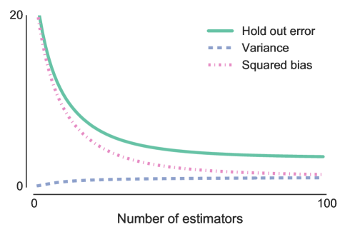
Figure 4.3: Bias-variance decomposition of a boosting ensemble minimizing the square loss with an increasing number of weak models on the Friedman1 dataset. The hold out error, variance and squared bias are averaged over 100 independent learning and testing sets of respective size 300 and 20000 samples.

We present the adaptive boosting and its variants in Section 16.1, which directly solve Equation 4.31, and the functional gradient boosting approach in Section 16.2, which approximately solves Equation 4.31 through the loss gradient.

16.1   Adaboost and variants

One of the most popular and influential boosting algorithms is the “AdaBoost” algorithm Freund and Schapire (1997). This supervised learning algorithm aims to solve binary classification tasks with $\mathcal{Y}=\{-1,1\}$. The algorithm generates iteratively an ensemble of estimators $\{f_{m}\}_{m=1}^{M}$ by minimizing the exponential loss function:

$$\ell_{\exp}(y,y^{\prime})=\exp(-yy^{\prime})),$$ (4.32)

assuming a binary response of the weak models $f_{m}(x)\in\{-1,1\}\,\forall m$.

The prediction of an unseen sample $f(x)$ by an AdaBoost ensemble is a majority vote from its members:

$$f(x)=\operatorname{sign}\left(\sum_{m=1}^{M}\alpha_{m}f_{m}(x)\right),$$ (4.33)

where the $\{\alpha_{m}\}_{m=1}^{M}$ are constant weights indicating the contribution of a model $f_{m}$ to solve the binary classification task. The $\operatorname{sign}$ operator transforms the sum into an appropriate output value ($\mathcal{Y}=\{-1,1\}$).

Given a learning set $\mathcal{L}=((x^{i},y^{i})\in\mathcal{X}\times\{-1,1\})_{i=1}^{n}$, we iteratively fit a weak model $f_{m}$ over the learning set $\mathcal{L}$ by making the weak learner focuses on each sample with a weight $(w^{i})_{i=1}^{n}$. The higher the value of $w^{i}$, the more the algorithm will concentrate to predict correctly the $i$-th sample. To design this algorithm, we need to answer to the following questions: (i) how to assess the contribution $\alpha_{m}$ of the $m$-th model $f_{m}$ to the ensemble and (ii) how to update the weight $w^{i}$ to reduce iteratively the exponential loss.

We can write the resubtitution error of the exponential loss as

$$\frac{1}{n}\sum_{i=1}^{n}\ell_{\exp}\left(y^{i},\sum_{l=1}^{m-1}\alpha_{l}f_{l}(x^{i})+\alpha_{m}f_{m}(x^{i})\right)$$

$$=\frac{1}{n}\sum_{i=1}^{n}\exp\left(-y^{i}\left(\sum_{l=1}^{m-1}\alpha_{l}f_{l}(x^{i})+\alpha_{m}f_{m}(x^{i})\right)\right)$$ (4.34)

$$=\frac{1}{n}\sum_{i=1}^{n}\exp\left(-y^{i}\left(\sum_{l=1}^{m-1}\alpha_{l}f_{l}(x^{i}))\right)\right)\exp\left(-y^{i}\alpha_{m}f_{m}(x^{i})\right)~$$ (4.35)

$$=\frac{1}{n}\sum_{i=1}^{n}\ell_{\exp}\left(y,\sum_{l=1}^{m-1}\alpha_{l}f_{l}(x^{i})\right)\exp(-y^{i}\alpha_{m}f_{m}(x^{i}))$$ (4.36)

$$=\sum_{i=1}w^{i}\exp(-y^{i}\alpha_{m}f_{m}(x^{i}))$$ (4.37)

with

$$w^{i}=\frac{1}{n}\ell_{\exp}\left(y,\sum_{l=1}^{m-1}\alpha_{l}f_{l}(x^{i})\right)\forall i.$$ (4.38)

Note that the weight computation is expressible as a recursive equation starting with $w^{i}=1/n$:

$$w^{i}\leftarrow w^{i}\exp\left(\alpha_{m}1(y^{i}\not=f_{m}(x^{i}))\right).$$ (4.39)

The sample weight $w^{i}$ highlights how well the $i$-th sample is predicted by the $m-1$ first estimators of the boosting ensemble. A zero weight $w^{i}$ means that the $i$-th sample is perfectly predicted. The $m$-th estimators should thus focus on the sample with high weight $w^{i}$ to reduce the resubtitution error. Otherwise, it should minimize the weighted resubstitution error.

Let us now separate the resubtitution error of the correctly classified points from the misclassified ones:

$$\sum_{i=1}^{n}w^{i}\exp(-y^{i}\alpha_{m}f_{m}(x^{i}))$$

$$= \sum_{i=1}^{n}w^{i}\exp(-\alpha_{m})1(y^{i}=f_{m}(x^{i}))+\exp(\alpha_{m})1(y^{i}\not=f_{m}(x^{i}))$$ (4.40)

By derivating the last equation with respect to $\alpha_{m}$ and setting the derivative to zero, the $\alpha_{m}$ minimizing the resubtitution error of the exponential loss is

$$\alpha_{m}=\log\left(\frac{1-\text{err}_{m}}{\text{err}_{m}}\right)$$ (4.41)

with

$$\text{err}_{m}=\frac{1}{2}\frac{\sum_{i=1}^{n}w^{i}1(y^{i}\not=f_{m}(x^{i}))}{\sum_{i=1}^{n}w^{i}}.$$ (4.42)

The optimization of the constant $\alpha_{m}$ means that the resubstitution error is upper bounded and can not increase with the size of the ensemble on the learning set.

Putting everything together, we obtain the AdaBoost algorithm (see Algorithm 1). Many extensions and enhancements of this fundamental idea have been proposed. If the weak model is able to predict a probability estimate, Friedman et al. (2000) have proposed an appropriate extension called “Real Adaboost” by contrast to Algorithm 1 which they call “Discrete Adaboost”.

Algorithm 1 AdaBoost.M1 for binary classification $\mathcal{Y}=\{-1,1\}$.

1:function Adaboost($\mathcal{L}=\{x^{i},y^{i}\in\mathcal{X}\times\mathcal{Y}\}_{i=1}^{n}$)

2:     Initialize the sample weights $w^{i}\leftarrow 1/n\,\forall i\in~\{1,\ldots,n\}$.

3:     for $m$ = 1 to $M$ do

4:         Fit a model $f_{m}(x)$ to the learning set $\mathcal{L}$ and $(w^{i})_{i=1}^{n}$.

5:         Compute the weighted error rate

$$\qquad\text{err}_{m}\leftarrow\frac{\sum_{i=1}^{n}w^{i}1(y^{i}\not=f_{m}(x^{i}))}{\sum_{i=1}^{n}w^{i}}.$$

6:         Compute $\alpha_{m}\leftarrow\frac{1}{2}\log\left(\frac{1-\text{err}_{m}}{\text{err}_{m}}\right)$.

7:         Update the weights

$$\qquad w^{i}\leftarrow w^{i}\exp\left(\alpha_{m}1(y^{i}\not=f_{m}(x^{i}))\right).$$

8:     end for

9:     return $\hat{f}(x)=\operatorname{sign}\left(\sum_{m=1}^{M}\alpha_{m}f_{m}(x)\right)$

10:end function

A direct multi-class extension, called AdaBoost.M1, of the AdaBoost algorithm is to use a multi-class weak learner instead of a binary one. The AdaBoost.M1 ensemble predicts a new sample through:

$$f(x)=\arg\max_{k\in\mathcal{Y}}\sum_{m=1}^{M}\alpha_{m}1(f_{m}(x)=k).$$ (4.43)

An improvement over this approach is to directly minimize the multi-class exponential loss as in the SAMME algorithm Zhu et al. (2009). It replaces the line 6 of Algorithm 1 by

$$\alpha_{m}\leftarrow\frac{1}{2}\log\left(\frac{1-\text{err}_{m}}{\text{err}_{m}}\right)+\log(|\mathcal{Y}|-1)$$ (4.44)

We can minimize other losses than the exponential loss during the ensemble growth, such as the logistic loss $\ell_{logistic}(y,y^{\prime})=\log(1+\exp(-2yy^{\prime}))$ with the LogitBoost algorithm Collins et al. (2002) for binary classification tasks; the Hamming loss $\ell_{\text{Hamming}}(y,y^{\prime})=\sum_{j=1}^{n}1(y_{j}\not=y^{\prime}_{j})$ leading to the AdaBoost.MH algorithm Schapire and Singer (2000) and the pairwise ranking loss $\ell_{\text{ranking}}$

$$\ell_{\text{ranking}}(y,y^{\prime})=\frac{1}{|y^{i}|}\frac{1}{d-|y^{i}|}\left|\left\{(k,l):y^{\prime i}_{k}<y^{\prime i}_{l},y^{i}_{k}=1,y^{i}_{l}=0\right\}\right|$$

leading to the AdaBoost.MR algorithm Schapire and Singer (2000) for multi-label classification tasks and also a wide range of regression losses as proposed in Drucker (1997) for regression tasks.

Remark 16.10.

How to take into account sample weights in supervised learning algorithms? For a set of learning samples $\left((x^{i},y^{i})\in\left(\mathcal{X}\times\mathcal{Y}\right)\right)_{i=1}^{n}$ and a set of weights $(w^{i}\in\mathbb{R}^{+})_{i=1}^{n}$, the weighted resubtitution error is given by

$$\text{Resubstitution error}=\frac{\sum_{i=1}^{n}w^{i}\ell(f(x^{i}),y^{i})}{\sum_{i=1}^{n}w^{i}}.$$ (4.45)

Extending supervised learning algorithms to support sample weights means that we have to modify the learning algorithm so as to minimize the weighted resubtitution error:

• For linear models, we will minimize the weighted average of a given loss $\ell:\mathcal{Y}\times\mathcal{Y}\rightarrow\mathbb{R}^{+}$ over the learning set $\mathcal{L}=\{(x^{i},y^{i})\in\mathcal{X}\times\mathcal{Y}\}_{i=1}^{n}$

  $$\min_{\beta_{0},\beta}\sum_{i=1}^{n}w^{i}L(y^{i},\beta_{0}+\beta^{T}x),$$ (4.46)

  where the $w^{i}\in\mathbb{R}^{+}$ are the weight associated to each sample. There is an analytical solution in the case of a $\ell_{2}$ norm regularization penalty and algorithms for a $\ell_{1}$ regularization penalty can be easily extended to accommodate for the weights.

• For a decision tree, we will use a weighted impurity criterion and a weight-aware leaf labelling rule assignment procedure. It also allows new stopping rule based on sample-weight, such as a minimal total weight to split a node.

• For a $k$-nearest neighbors, we will store the sample weight during fit and we will predict an unseen sample through a weighted aggregation of the nearest neighbors.

Conversely, to support unweighted supervised learning task with a weight-aware implementation, we can set the sample weights to a constant such as $w^{i}=1/n\,\forall i$ prior the model training.

16.2   Functional gradient boosting

The AdaBoost algorithm has an analytical and closed-form solution to Equation 4.31 with the exponential loss. However, we would like to build boosting ensembles when such closed-form solutions are not available. Functional gradient boosting, a forward stagewise additive approach, approximately solves Equation 4.31 for a given loss $\ell:\mathcal{Y}\times\mathcal{Y}\rightarrow\mathbb{R}^{+}$ by sequentially adding new basis function $f_{m}$, a regression model, with a weight $\alpha_{m}$ without modifying the previous models.

If we want to add a new model $f_{m}$ to a boosting ensemble with $m-1$ models while minimizing the square loss, the loss for a sample $(x,y)$ is given by

$$\ell(y,f(x)) =\frac{1}{2}(y-f(x))^{2}$$ (4.47)

$$=\frac{1}{2}(y-\sum_{l=1}^{m-1}\alpha_{l}f_{l}(x)-\alpha_{m}f_{m}(x))^{2}~$$ (4.48)

$$=\frac{1}{2}(r_{m}(x)-\alpha_{m}f_{m}(x))^{2}$$ (4.49)

where $r_{m}(x)=y-\sum_{l=1}^{m-1}\alpha_{l}f_{l}(x)$ is the remaining residual of the $m-1$ models to predict a sample $x$. Thus for the square loss, we can add a new models $f_{m}$ by fitting the new model on the residuals left by the $m-1$ previous models. This approach is called least square regression boosting.

Solving Equation 4.31 is difficult for general loss functions. It requires to be able to expand a new basis function $f_{m}$ while minimizing the chosen loss function. For instance in the context of decision trees, it would require a specific splitting criterion and a leaf labelling rule minimizing the chosen loss.

Instead of solving Equation 4.31, Friedman (2001) proposed a fast approximate solution for arbitrary differentiable losses inspired from numerical optimization. We can re-write the loss function minimization as

$$\hat{f}=\arg\min_{f}\ell(f)=\min_{f}\sum_{(x,y)\in\mathcal{L}}\ell(y,f(x)).$$ (4.50)

with the constraint that $f$ is a sum of supervised learning models. Ignoring this constraint, the Equation 4.50 is an unconstrained minimization problem with $f\in\mathbb{R}^{n}$ being a $n$-dimensional vector. Iterative solvers solve such minimization problems by correcting an initial estimate through a recursive equation. The final solution is a sum of vectors

$$\hat{f}=\sum_{m=0}^{M}h_{m},\quad h_{m}\in\mathbb{R}^{n},$$ (4.51)

where $h_{0}$ is the initial estimate. The construction of the sequence of $h_{0},\ldots,h_{m}$ depends on the chosen optimization algorithm.

The gradient boosting algorithm Friedman (2001) uses the same approach as the gradient descent method. The update rule of the gradient descent algorithm $h_{m}$ is of the form

$$h_{m}=-\rho_{m}g_{m}$$ (4.52)

where $\rho_{m}$ is a scalar and $g_{m}\in\mathbb{R}^{n}$ is the gradient of $L(f)$ with respect to $f$ evaluated at the current approximate solution $\hat{f}=\sum_{l=1}^{m-1}\rho_{l}h_{l}$:

$$g^{i}_{m}=\left[\frac{\partial}{\partial y^{\prime}}\ell(y^{i},y^{\prime})\right]_{y^{\prime}=\hat{f}}.$$ (4.53)

The scalar $\rho_{m}$ is the step length in the negative loss gradient direction $-g_{m}$ chosen so as to minimize the objective function $\ell(f)$:

$$\rho_{m}=\arg\min_{\rho\in\mathbb{R}}\ell(\hat{f}-\rho_{m}g_{m}).$$ (4.54)

Back to supervised learning, we can only compute the loss gradient for the training samples. To generalize to unseen data, the idea is to approximate the direction of the negative gradient using a regression model $g_{m}$ selected within a hypothesis space $\mathcal{H}$ of weak base-learners minimizing the square loss on the training data:

$$g_{m}=\arg\min_{g\in\mathcal{H}}\sum_{i=1}^{n}(-g_{m}^{i}-g(x^{i}))^{2}.$$ (4.55)

The gradient boosting approach can be summarized as follows: start at an initial constant estimate $\rho_{0}\in\mathbb{R}$, then iteratively follows the negative gradient of the loss $\ell$ as estimated by a regression model $g_{m}$ fitted over the training samples and make an optimal step length $\rho_{m}$ minimizing the loss $\ell$. The gradient boosting ensemble predicts an unseen sample through

$$f(x)=\rho_{0}+\sum_{m=1}^{M}\rho_{m}g_{m}(x).$$ (4.56)

The whole procedure is given in Algorithm 2. The algorithm is completely defined once we have (i) a starting model, usually the constant minimizing the chosen loss (line 4) and (ii) the gradient of the loss (line 2).

Algorithm 2 Gradient boosting algorithm

1:function GradientBoosting($\mathcal{L}=\{(x^{i},y^{i})\in\mathcal{X}\times\mathcal{Y}\}_{i=1}^{n};\ell;\mathcal{H};M$)

2:     $f_{0}(x)=\rho_{0}=\arg\min_{\rho\in\mathbb{R}}\sum_{i=1}^{n}\ell(y^{i},\rho)$.

3:     for $m$ = 1 to $M$ do

4:         Compute the loss gradient for the training set points

$$\quad g_{m}^{i}=\left[\frac{\partial}{\partial y^{\prime}}\ell(y^{i},y^{\prime})\right]_{y^{\prime}=f_{m-1}(x)}\forall i\in\left\{1,\ldots,n\right\}.$$

5:         Find a correlated direction to the loss gradient

$$\quad g_{m}=\arg\min_{g\in~\mathcal{H}}\sum_{i=1}^{n}(-g_{m}^{i}-g(x^{i}))^{2}.$$

6:         Find an optimal step length in the direction $g_{m}$

$$\quad\rho_{m}=\arg\min_{\rho\in\mathbb{R}}\sum_{i=1}^{n}\ell\left(y^{i},f_{m-1}(x^{i})+\rho g_{m}(x^{i})\right).$$

7:         $f_{m}(x)=f_{m-1}(x)+\mu\rho_{m}g_{m}(x)$.

8:     end for

9:     return $f_{M}(x)$

10:end function

We compute the optimal step length (line 6 of Algorithm 2) either analytically as for the square loss or numerically using, e.g., the Brent’s method Brent (2013), a robust root-finding method allowing to minimize single unconstrained optimization problem, as for the logistic loss. Friedman (2001) advises to use one step of the Newton–Raphson method. However, the Newton–Raphson algorithm might not converge if the first and second derivative of the loss are small. These conditions occurs frequently in highly imbalanced supervised learning tasks.

A learning rate $\mu\in(0,1]$ is often added to shrink the size of the gradient step $\rho_{m}$ in the residual space in order to avoid overfitting the the training samples. Another possible modification is to induce randomization, e.g. by subsampling without replacement the samples available (from all learning samples) at each iteration Friedman (2002).

Table 4.1 gives an overview of regression and classification losses with their gradients, while Table 4.2 gives the starting constant models minimizing losses. The square loss in regression and the exponential loss in classification leads to nice gradient boosting algorithm (respectively the least square regression boosting algorithm and the exponential classification boosting algorithm Zhu et al. (2009)). However, these losses are not robust to outlier. More robust losses can be used such as the absolute loss in regression and the logistic loss or the hinge loss in classification.

Table 4.1: Regression loss ($\mathcal{Y}=\mathbb{R}$) and binary classification loss ($\mathcal{Y}=\{-1,1\}$) their derivative with respect to a basis function $f(x)$.

Regression	$\ell(y,y^{\prime})$	$-\partial{}\ell(y,y^{\prime})/\partial{}y^{\prime}$
Square	$\frac{1}{2}(y-y^{\prime})^{2}$	$y-y^{\prime}$
Absolute	$|y-y^{\prime}|$	$\operatorname{sign}(y-y^{\prime})$
Classification	$\ell(y,y^{\prime})$	$-\partial{}\ell(y,y^{\prime})/\partial{}y^{\prime}$
Exponential	$\exp(-yy^{\prime})$	$-y\exp(-yy^{\prime})$
Logistic	$\log(1+\exp(-2yy^{\prime}))$	$\frac{2y}{1+\exp(2yy^{\prime})}$
Hinge	$\max(0,1-yy^{\prime})$	$-y1(yy^{\prime}<1)$

Table 4.2: Constant minimizers of regression losses ($\mathcal{Y}=\mathbb{R}$) and binary classification losses ($\mathcal{Y}=\{-1,1\}$) given a set of samples $\mathcal{L}=\{(x^{i},y^{i})\in\mathcal{X}\times\mathcal{Y}\}_{i=1}^{n}$.

Regression
Square	$f_{0}(x)=\frac{1}{n}\sum_{i=1}^{n}y^{i}$
Absolute	$f_{0}(x)=\text{median}(\{y^{i}\}_{i=1}^{n})$
Classification
Exponential	$f_{0}(x)=\log\left(\frac{\sum_{i=1}^{n}1(y^{i}=1)}{\sum_{i=1}^{n}1(y^{i}=-1)}\right)$
Logistic	$f_{0}(x)=\log\left(\frac{\sum_{i=1}^{n}1(y^{i}=1)}{\sum_{i=1}^{n}1(y^{i}=-1)}\right)$
Hinge	$f_{0}(x)=\operatorname{sign}\left(\frac{1}{n}\sum_{i=1}^{n}1(y^{i}=1)-\frac{1}{2}\right)$

Part II   Learning in compressed space through random projections

Random forests with random projections of the output space for high dimensional multi-label classification

Remark 16.11.

Outline We adapt the idea of random projections applied to the output space, so as to enhance tree-based ensemble methods in the context of multi-label classification. We show how learning time complexity can be reduced without affecting computational complexity and accuracy of predictions. We also show that random output space projections may be used in order to reach different bias-variance tradeoffs, over a broad panel of benchmark problems, and that this may lead to improved accuracy while reducing significantly the computational burden of the learning stage.

This chapter is based on previous work published in

Arnaud Joly, Pierre Geurts, and Louis Wehenkel. Random forests with random projections of the output space for high dimensional multi-label classification. In Machine Learning and Knowledge Discovery in Databases, pages 607–622. Springer Berlin Heidelberg, 2014.

Within supervised learning, the goal of multi-label classification is to train models to annotate objects with a subset of labels taken from a set of candidate labels. Typical applications include the determination of topics addressed in a text document, the identification of object categories present within an image, or the prediction of biological properties of a gene. In many applications, the number of candidate labels may be very large, ranging from hundreds to hundreds of thousands Agrawal et al. (2013) and often even exceeding the sample size Dekel and Shamir (2010). The very large scale nature of the output space in such problems poses both statistical and computational challenges that need to be specifically addressed.

A simple approach to multi-label classification problems, called binary relevance, is to train independently a binary classifier for each label. Several more complex schemes have however been proposed to take into account the dependencies between the labels (see Section 4.5). In the context of tree-based methods, one way is to train multi-output trees (see Section 13), i.e. trees that can predict multiple outputs at once. With respect to binary relevance, the multi-output tree approach has the advantage of building a single model for all labels. It can thus potentially take into account label dependencies and reduce memory requirements for the storage of the models. An extensive experimental comparison Madjarov et al. (2012) shows that this approach compares favorably with other approaches, including non tree-based methods, both in terms of accuracy and computing times. In addition, multi-output trees inherit all intrinsic advantages of tree-based methods, such as robustness to irrelevant features, interpretability through feature importance scores, or fast computations of predictions, that make them very attractive to address multi-label problems. The computational complexity of learning multi-output trees is however similar to that of the binary relevance method. Both approaches are indeed $O(pdn\log n)$, where $p$ is the number of input features, $d$ the number of candidate output labels, and $n$ the sample size; this is a limiting factor when dealing with large sets of candidate labels.

One generic approach to reduce computational complexity is to apply some compression technique prior to the training stage to reduce the number of outputs to a number $q$ much smaller than the total number $d$ of labels. A model can then be trained to make predictions in the compressed output space and a prediction in the original label space can be obtained by decoding the compressed prediction. As multi-label vectors are typically very sparse, one can expect a drastic dimensionality reduction by using appropriate compression techniques. This idea has been explored for example in Hsu et al. (2009) using compressed sensing, and in Cisse et al. (2013) using bloom filters, in both cases using regularized linear models as base learners. The approach obviously reduces computing times for training the model. Random projections are also exploited in Tsoumakas et al. (2014) for multi-target regression. In this latter work however, they are not used to improve computing times by compression but instead to improve predictive performance. Indeed, more (sparse) random projections are computed than there are outputs and they are used each as an output to train some single target regressor. As in Hsu et al. (2009); Cisse et al. (2013), the predictions of the regressors need to be decoded at prediction time to obtain a prediction in the original output space. This is achieved in Tsoumakas et al. (2014) by solving an overdetermined linear system.

In this chapter, we explore the use of random output space projections for large-scale multi-label classification in the context of tree-based ensemble methods. We first explore the idea proposed for linear models in Hsu et al. (2009) with random forests: a (single) random projection of the multi-label vector to a $q$-dimensional random subspace is computed and then a multi-output random forest is grown based on score computations using the projected outputs. We exploit however the fact that the approximation provided by a tree ensemble is a weighted average of output vectors from the training sample to avoid the decoding stage: at training time all leaf labels are directly computed in the original multi-label space. We show theoretically and empirically that when $q$ is large enough, ensembles grown on such random output spaces are equivalent to ensembles grown on the original output space. When $d$ is large enough compared to $n$, this idea hence may reduce computing times at the learning stage without affecting accuracy and computational complexity of predictions.

Next, we propose to exploit the randomization inherent to the projection of the output space as a way to obtain randomized trees in the context of ensemble methods: each tree in the ensemble is thus grown from a different randomly projected subspace of dimension $q$. As previously, labels at leaf nodes are directly computed in the original output space to avoid the decoding step. We show, theoretically, that this idea can lead to better accuracy than the first idea and, empirically, that best results are obtained on many problems with very low values of $q$, which leads to significant computing time reductions at the learning stage. In addition, we study the interaction between input randomization (à la Random Forests) and output randomization (through random projections), showing that there is an interest, both in terms of predictive performance and in terms of computing times, to optimally combine these two ways of randomization. All in all, the proposed approach constitutes a very attractive way to address large-scale multi-label problems with tree-based ensemble methods.

The rest of the chapter is structured as follows: Section 17 presents the proposed algorithms and their theoretical properties; Section 18 analyses the proposed algorithm from a bias-variance perspective; Section 19 provides the empirical validations, whereas Section 20 discusses our work and provides further research directions.

17   Methods

We first present how we propose to exploit random projections to reduce the computational burden of learning single multi-output trees in very high-dimensional output spaces. Then we present and compare two ways to exploit this idea with ensembles of trees.

17.1   Multi-output regression trees in randomly projected output spaces

The multi-output single tree algorithm described in Chapter 3 requires the computation of the sum of impurity criterion, such as the variance (or Gini), at each tree node and for each candidate split. When $\mathcal{Y}$ is very high-dimensional, this computation constitutes the main computational bottleneck of the algorithm. We thus propose to approximate variance computations by using random projections of the output space. The multi-output regression tree algorithm is modified as follows (denoting by $\mathcal{L}$ the learning sample $\mathcal{L}=((x^{i},y^{i})\in\mathcal{X}\times\mathcal{Y})_{i=1}^{n}$):

• First, a projection matrix $\Phi$ of dimension $q\times d$ is randomly generated.

• A new dataset $\mathcal{L}_{m}=((x^{i},\Phi y^{i}))_{i=1}^{n}$ is constructed by projecting each learning sample output using the projection matrix $\Phi$.

• A tree (structure) $\mathcal{T}_{m}$ is grown using the projected learning sample $\mathcal{L}_{m}$.

• Predictions $\hat{y}$ at each leaf of $\cal T$ are computed using the corresponding outputs in the original output space.

The resulting tree is exploited in the standard way to make predictions: an input vector $x$ is propagated through the tree until it reaches a leaf from which a prediction $\hat{y}$ in the original output space is directly retrieved.

If $\Phi$ satisfies the Jonhson-Lindenstrauss lemma (Equation 2.86), the following theorem shows that variance computed in the projected subspace is an $\epsilon$-approximation of the variance computed over the original space.

Theorem 17.12.

Given $\epsilon>0$, a sample $(y^{i})_{i=1}^{n}$ of $n$ points $y\in\mathbb{R}^{d}$, and a projection matrix $\Phi\in\mathbb{R}^{q\times d}$ such that for all $i,j\in\{1,\ldots,n\}$ the condition given by Equation 2.86 holds, we have also:

$$(1-\epsilon)\operatorname{Var}((y^{i})_{i=1}^{n})\leq\operatorname{Var}((\Phi y^{i})_{i=1}^{n})\leq(1+\epsilon)\operatorname{Var}((y^{i})_{i=1}^{n}).$$ (5.1)

Proof 17.13.

The sum of the variances of $n$ observations drawn from a random vector $y\in\mathbb{R}^{d}$ can be interpreted as a sum of squared euclidean distances between the pairs of observations

$$\operatorname{Var}((y^{i})_{i=1}^{n})=\frac{1}{2n^{2}}\sum_{i=1}^{n}\sum_{j=1}^{n}||y^{i}-y^{j}||^{2}.$$ (5.2)

Starting from the defition of the variance, we have

$$\operatorname{Var}((y^{i})_{i=1}^{n})$$

$$\stackrel{{\scriptstyle\mbox{\tiny def}}}{{=}}\frac{1}{n}\sum_{i=1}^{n}||y^{i}-\frac{1}{n}\sum_{j=1}^{n}y^{j}||^{2}$$ (5.3)

$$=\frac{1}{n}\sum_{i=1}^{n}(y^{i}-\frac{1}{n}\sum_{j=1}^{n}y^{j})^{T}(y^{i}-\frac{1}{n}\sum_{k=1}^{n}y^{k})$$ (5.4)

$$=\frac{1}{n}\sum_{i=1}^{n}\left({y^{i}}^{T}y^{i}-\frac{2}{n}\sum_{j=1}^{n}{y^{i}}^{T}y^{j}+\frac{1}{n^{2}}\sum_{j=1}^{n}\sum_{k=1}^{n}{y^{j}}^{T}y^{k}\right)$$ (5.5)

$$=\frac{1}{n}\sum_{i=1}^{n}{y^{i}}^{T}y^{i}-\frac{2}{n^{2}}\sum_{i=1}^{n}\sum_{j=1}^{n}{y^{i}}^{T}y^{j}+\frac{1}{n^{2}}\sum_{j=1}^{n}\sum_{k=1}^{n}{y^{j}}^{T}y^{k}$$ (5.6)

$$=\frac{1}{n}\sum_{i=1}^{n}{y^{i}}^{T}y^{i}-\frac{1}{n^{2}}\sum_{i=1}^{n}\sum_{j=1}^{n}{y^{i}}^{T}y^{j}$$ (5.7)

$$=\frac{1}{2n}\sum_{i=1}^{n}{y^{i}}^{T}y^{i}+\frac{1}{2n}\sum_{j=1}^{n}{y^{j}}^{T}y^{j}-\frac{1}{n^{2}}\sum_{i=1}^{n}\sum_{j=1}^{n}{y^{i}}^{T}y^{j}$$ (5.8)

$$=\frac{1}{2n^{2}}\sum_{i=1}^{n}\sum_{j=1}^{n}{y^{i}}^{T}y^{i}+\frac{1}{2n^{2}}\sum_{i=1}^{n}\sum_{j=1}^{n}{y^{j}}^{T}y^{j}-\frac{1}{n^{2}}\sum_{i=1}^{n}\sum_{j=1}^{n}{y^{i}}^{T}y^{j}$$ (5.9)

$$=\frac{1}{2n^{2}}\sum_{i=1}^{n}\sum_{j=1}^{n}\left({y^{i}}^{T}y^{i}+{y^{j}}^{T}y^{j}-2{y^{i}}^{T}y^{j}\right)$$ (5.10)

$$=\frac{1}{2n^{2}}\sum_{i=1}^{n}\sum_{j=1}^{n}||y^{i}-y^{j}||^{2}.$$ (5.11)

From the Johnson-Lindenstrauss Lemma we have for any $i,j$

$$(1-\epsilon)||y^{i}-y^{j}||^{2}\leq||\Phi y^{i}-\Phi y^{j}||^{2}\leq(1+\epsilon)||y^{i}-y^{j}||^{2}.$$ (5.12)

By summing the three terms of Equation 5.12 over all pairs $i,j$ and dividing by $1/(2n^{2})$ and by then using Equation 5.2, we get Equation 5.1.

As a consequence, any split score approximated from the randomly projected output space will be $\epsilon$-close to the unprojected scores in any subsample of the complete learning sample. Thus, if the condition given by Equation 2.86) is satisfied for a sufficiently small $\epsilon$ then the tree grown from the projected data will be identical to the tree grown from the original data.

For a given size $q$ of the projection subspace, the complexity is reduced from $O(dn)$ to $O(qn)$ for the computation of one split score and thus from $O(dpn\log n)$ to $O(qpn\log n)$ for the construction of one full (balanced) tree, where one can expect $q$ to be much smaller than $d$ and at worst of $O(\epsilon^{-2}\log{n})$. The whole procedure requires to generate the projection matrix and to project the training data. These two steps are respectively $O(dq)$ and $O(ndq)$ but they can often be significantly accelerated by exploiting the sparsity of the projection matrix and/or of the original output data, and they are called only once before growing the tree.

All in all, this means that when $d$ is sufficiently large, the random projection approach may allow us to significantly reduce tree building complexity from $O(dpn\log n)$ to $O(qpn\log n+ndq)$, without impact on predictive accuracy (see Section 19, for empirical results).

17.2   Exploitation in the context of tree ensembles

The idea developed in the previous section can be directly exploited in the context of ensembles of randomized multi-output regression trees. Instead of building a single tree from the projected learning sample, one can grow a randomized ensemble of them. This “shared subspace” algorithm is described in pseudo-code in Algorithm 1.

Algorithm 1 Grow $t$ decision trees on a single shared subspace $\Phi$ using learning samples $\mathcal{L}=((x^{i},y^{i})\in(\mathbb{R}^{p}\times\mathbb{R}^{d}))_{i=1}^{n}$

1:function GrowForestSharedOutputSubspace($\mathcal{L}$,$t$)

2:     Generate a sub-space $\Phi\in\mathbb{R}^{q\times d}$;

3:     for $j=1$ to $t$ do

4:         Build a tree structure $\mathcal{T}_{j}$ using $((x^{i},\Phi y^{i}))_{i=1}^{n}$;

5:         Label the leaves of $\mathcal{T}_{j}$ using $((x^{i},y^{i}))_{i=1}^{n}$;

6:         Add the labelled tree $\mathcal{T}_{j}$ to the ensemble;

7:     end for

8:end function

Another idea is to exploit the random projections used so as to introduce a novel kind of diversity among the different trees of an ensemble. Instead of building all the trees of the ensemble from a same shared output-space projection, one could instead grow each tree in the ensemble from a different output-space projection. Algorithm 2 implements this idea in pseudo-code. The randomization introduced by the output space projection can of course be combined with any existing randomization scheme to grow ensembles of trees. In this chapter, we will consider the combination of random projections with the randomizations already introduced in Random Forests and Extra Trees. The interplay between these different randomizations will be discussed theoretically in the next subsection by a bias/variance analysis and empirically in Section 19. Note that while when looking at single trees or shared ensembles, the size $q$ of the projected subspace should not be too small so that condition (Equation 2.86) is satisfied, the optimal value of $q$ when projections are randomized at each tree is likely to be smaller, as suggested by the bias/variance analysis in the next section.

Algorithm 2 Grow $t$ decision trees on individual random subspaces $(\Phi_{j})_{j=1}^{t}$ using learning samples $\mathcal{L}=((x^{i},y^{i})\in(\mathbb{R}^{p}\times\mathbb{R}^{d}))_{i=1}^{n}$

1:function GrowForestOutputSubspace($\mathcal{L}$,$t$)

2:     for $j=1$ to $t$ do

3:         Generate a sub-space $\Phi_{j}\in\mathbb{R}^{q\times d}$;

4:         Build a tree structure $\mathcal{T}_{j}$ using $((x^{i},\Phi_{j}y^{i}))_{i=1}^{n}$;

5:         Label the leaves of $\mathcal{T}_{j}$ using $((x^{i},y^{i}))_{i=1}^{n}$;

6:         Add the labelled tree $\mathcal{T}_{j}$ to the ensemble;

7:     end for

8:end function

From the computational point of view, the main difference between these two ways of transposing random-output projections to ensembles of trees is that in the case of Algorithm 2, the generation of the projection matrix $\Phi$ and the computation of projected outputs is carried out $t$ times, while it is done only once for the case of Algorithm 1. These aspects will be empirically evaluated in Section 19.

18   Bias/variance analysis

In this section, we adapt the bias/variance analysis carried out in Section 15.1 to take into account random output projections. The details of the derivations are reported in Section 18.1 for a single tree and in Section 18.2 for an ensemble of $t$ randomized trees.

Let us denote by $f_{\mathcal{L},\phi,\sigma}(.):{\cal X}\rightarrow\mathbb{R}^{d}$ a single multi-output tree obtained from a projection matrix $\phi$ (below we use $\Phi$ to denote the corresponding random variable), where $\sigma$ is the value of a random variable $\varsigma$ capturing the random perturbation scheme used to build this tree (e.g., bootstrapping and/or random input space selection). The square error of this model at some point $x\in{\cal X}$ is defined by:

$$Err(f_{\mathcal{L},\phi,\sigma}(x))\stackrel{{\scriptstyle\text{def}}}{{=}}\operatorname{E}_{Y|x}\{||Y-f_{\mathcal{L},\phi,\sigma}(x))||^{2}\},$$

and its average can decomposed in its residual error, (squared) bias, and variance terms denoted:

$$\operatorname{E}_{\mathcal{L},\Phi,\varsigma}\{Err(f_{\mathcal{L},\phi,\varsigma}(x))\}=\sigma^{2}_{R}(x)+B^{2}(x)+V(x)$$

where the variance term $V(x)$ can be further decomposed as the sum of the following three terms:

$$V_{\mathcal{L}}(x) = \operatorname{Var}_{\mathcal{L}}\{\operatorname{E}_{\Phi,\varsigma|\mathcal{L}}\{f_{\mathcal{L},\phi,\varsigma}(x)\}\}$$

$$V_{Algo}(x) = \operatorname{E}_{\mathcal{L}}\{\operatorname{E}_{\Phi|\mathcal{L}}\{\operatorname{Var}_{\varsigma|\mathcal{L},\Phi}\{f_{\mathcal{L},\phi,\varsigma}(x)\}\}\},$$

$$V_{Proj}(x) = \operatorname{E}_{\mathcal{L}}\{\operatorname{Var}_{\Phi|\mathcal{L}}\{\operatorname{E}_{\varsigma|\mathcal{L},\Phi}\{f_{\mathcal{L},\phi,\varsigma}(x)\}\}\},$$

that measure errors due to the randomness of, respectively, the learning sample, the tree algorithm, and the output space projection (see Section 18.1).

Approximations computed respectively by Algorithm 1 and Algorithm 2 take the following forms:

• $f_{1;\mathcal{L},\sigma^{t},\phi}(x)=\frac{1}{t}\sum_{i=1}^{t}f_{\mathcal{L},\phi,\sigma_{i}}(x)$

• $f_{2;\mathcal{L},\sigma^{t},\phi^{t}}(x)=\frac{1}{t}\sum_{i=1}^{t}f_{\mathcal{L},\phi_{i},\sigma_{i}}(x),$

where $\sigma^{t}=(\epsilon_{1},\ldots,\epsilon_{t})$ and $\phi^{t}=(\phi_{1},\ldots,\phi_{t})$ are vectors of i.i.d. values of the random variables $\varsigma$ and $\Phi$ respectively.

We are interested in comparing the average errors of these two algorithms, where the average is taken over all random parameters (including the learning sample). We show that these can be decomposed as follows (see Section 18.2):

$$\operatorname{E}_{\mathcal{L},\Phi,\varsigma^{t}}\{Err(f_{1;\mathcal{L},\Phi,\varsigma^{t}}(x))\}$$

$$=\sigma^{2}_{R}(x)+B^{2}(x)+V_{\mathcal{L}}(x)+\frac{V_{Algo}(x)}{t}+V_{Proj}(x),$$

$$\operatorname{E}_{\mathcal{L},\Phi^{t},\varsigma^{t}}\{Err(f_{2;\mathcal{L},\Phi^{t},\varsigma^{t}}(x))\}$$

$$=\sigma^{2}_{R}(x)+B^{2}(x)+V_{\mathcal{L}}(x)+\frac{V_{Algo}(x)+V_{Proj}(x)}{t}.$$

From this result, it is hence clear that Algorithm 2 can not be worse, on the average, than Algorithm 1. If the additional computational burden needed to generate a different random projection for each tree is not problematic, then Algorithm 2 should always be preferred to Algorithm 1.

For a fixed level of tree randomization ($\varsigma$), whether the additional randomization brought by random projections could be beneficial in terms of predictive performance remains an open question that will be addressed empirically in the next section. Nevertheless, with respect to an ensemble grown from the original output space, one can expect that the output-projections will always increase the bias term, since they disturb the algorithm in its objective of reducing the errors on the learning sample. For small values of $q$, the average error will therefore decrease (with a sufficiently large number $t$ of trees) only if the increase in bias is compensated by a decrease of variance.

The value of $q$, the dimension of the projected subspace, that will lead to the best tradeoff between bias and variance will hence depend both on the level of tree randomization and on the learning problem. The more (resp. less) tree randomization, the higher (resp. the lower) could be the optimal value of $q$, since both randomizations affect bias and variance in the same direction.

18.1   Single random trees.

Let us denote by $f_{\mathcal{L},\phi,\sigma}:{\cal X}\rightarrow\mathbb{R}^{d}$ a single multi-output (random) tree obtained from a projection matrix $\phi$ (below we use $\Phi$ to denote the corresponding random variable), where $\sigma$ is the value of a random variable $\varsigma$ capturing the random perturbation scheme used to build this tree (e.g., bootstrapping and/or random input space selection). Denoting by $Err(f_{\mathcal{L},\phi,\sigma}(x))$ the square error of this model at some point $x\in{\cal X}$ defined by:

$$\operatorname{E}_{P_{\mathcal{Y}|\mathcal{X}}}\{||y-f_{\mathcal{L},\phi,\sigma}(x)||^{2}\}.$$ (5.13)

The average of this square error can decomposed as follows:

$$\operatorname{E}_{\mathcal{L},\Phi,\varsigma}\{Err(f_{\mathcal{L},\phi,\sigma}(x))\}$$

$$= \sigma^{2}_{R}(x)+||f_{\text{Bayes}}(x)-\bar{f}(x)||^{2}+\operatorname{Var}_{\mathcal{L},\Phi,\varsigma}\{f_{\mathcal{L},\phi,\sigma}(x)\},$$

where

$$\bar{f}(x) \stackrel{{\scriptstyle\text{def}}}{{=}}\operatorname{E}_{\mathcal{L},\Phi,\varsigma}\{f_{\mathcal{L},\phi,\varsigma}(x)\}~$$

$$f_{\text{Bayes}}(x) =E_{Y|x}\{Y\}$$

$$\operatorname{Var}_{\mathcal{L},\Phi,\varsigma}\{f_{\mathcal{L},\phi,\varsigma}(x)\} \stackrel{{\scriptstyle\text{def}}}{{=}}E_{\mathcal{L},\Phi,\varsigma}\{||f_{\mathcal{L},\phi,\varsigma}(x)-\bar{f}(x)||^{2}\}.$$

The three terms of this decomposition are respectively the residual error, the bias, and the variance of this estimator (at $x$).

The variance term can be further decomposed as follows using the law of total variance:

$$\operatorname{Var}_{\mathcal{L},\Phi,\varsigma}\{f_{\mathcal{L},\phi,\varsigma}(x)\}$$ (5.14)

$$= \operatorname{Var}_{\mathcal{L}}\{E_{\Phi,\varsigma|\mathcal{L}}\{f_{\mathcal{L},\phi,\varsigma}(x)\}\}$$

$$+E_{\mathcal{L}}\{\operatorname{Var}_{\Phi,\varsigma|\mathcal{L}}\{f_{\mathcal{L},\phi,\varsigma}(x)\}\}.$$

The first term is the variance due to the learning sample randomization and the second term is the average variance (over $\mathcal{L}$) due to both the random forest randomization and the random output projection. By using the law of total variance a second time, the second term of Equation 5.14) can be further decomposed as follows:

$$\operatorname{E}_{\mathcal{L}}\{\operatorname{Var}_{\Phi,\varsigma|\mathcal{L}}\{f_{\mathcal{L},\phi,\varsigma}(x)\}\}$$

$$=\operatorname{E}_{\mathcal{L}}\{\operatorname{Var}_{\Phi|\mathcal{L}}\{\operatorname{E}_{\varsigma|\mathcal{L},\Phi}\{f_{\mathcal{L},\phi,\varsigma}(x)\}\}\}$$

$$\quad+\operatorname{E}_{\mathcal{L}}\{\operatorname{E}_{\Phi|\mathcal{L}}\{\operatorname{Var}_{\varsigma|\mathcal{L},\Phi}\{f_{\mathcal{L},\phi,\varsigma}(x)\}\}\}.$$ (5.15)

The first term of this decomposition is the variance due to the random choice of a projection and the second term is the average variance due to the random forest randomization. Note that all these terms are non negative. In what follows, we will denote these three terms respectively $V_{\mathcal{L}}(x)$, $V_{Algo}(x)$, and $V_{proj}(x)$. We thus have:

$$\operatorname{Var}_{\mathcal{L},\Phi,\varsigma}\{f_{\mathcal{L},\phi,\varsigma}(x)\}=V_{\mathcal{L}}(x)+V_{Algo}(x)+V_{Proj}(x),$$

with

$$V_{\mathcal{L}}(x) = \operatorname{Var}_{\mathcal{L}}\{\operatorname{E}_{\Phi,\varsigma|\mathcal{L}}\{f_{\mathcal{L},\phi,\varsigma}(x)\}\}$$

$$V_{Algo}(x) = \operatorname{E}_{\mathcal{L}}\{\operatorname{E}_{\Phi|\mathcal{L}}\{\operatorname{Var}_{\varsigma|\mathcal{L},\Phi}\{f_{\mathcal{L},\phi,\varsigma}(x)\}\}\},$$

$$V_{Proj}(x) = \operatorname{E}_{\mathcal{L}}\{\operatorname{Var}_{\Phi|\mathcal{L}}\{\operatorname{E}_{\varsigma|\mathcal{L},\Phi}\{f_{\mathcal{L},\phi,\varsigma}(x)\}\}\},$$

18.2   Ensembles of $t$ random trees.

When the random projection is fixed for all $t$ trees in the ensemble (Algorithm 1), the algorithm computes an approximation, denoted $f_{1}(x;\mathcal{L},\phi,\sigma^{t})$, that takes the following form:

$$f_{1;\mathcal{L},\phi,\sigma^{t}}(x)=\frac{1}{t}\sum_{i=1}^{t}f_{\mathcal{L},\phi,\sigma_{i}}(x),$$

where $\sigma^{t}=(\sigma_{1},\ldots,\sigma_{t})$ is a vector of i.i.d. values of the random variable $\varsigma$. When a different random projection is chosen for each tree (Algorithm 2), the algorithm computes an approximation, denoted by $f_{2}(x;\mathcal{L},\phi^{t},\sigma^{t})$, of the following form:

$$f_{2;\mathcal{L},\phi^{t},\sigma^{t}}(x)=\frac{1}{t}\sum_{i=1}^{t}f_{\mathcal{L},\phi_{i},\sigma_{i}}(x),$$

where $\phi^{t}=(\phi_{1},\ldots,\phi_{t})$ is also a vector of i.i.d. random projection matrices.

We would like to compare the average errors of these two algorithms with the average errors of the original single tree method, where the average is taken for all algorithms over their random parameters (that include the learning sample).

Given that all trees are grown independently of each other, one can show that the average models corresponding to each algorithm are equal:

$$\bar{f}(x) = \operatorname{E}_{\mathcal{L},\Phi,\varsigma^{t}}\{f_{1;\mathcal{L},\Phi,\varsigma^{t}}(x)\}$$

$$= \operatorname{E}_{\mathcal{L},\Phi^{t},\varsigma^{t}}\{f_{2;\mathcal{L},\Phi^{t},\varsigma^{t}}(x)\}.$$

They thus all have the exact same bias (and residual error) and differ only in their variance.

Using the same argument, the first term of the variance decomposition in (5.14), ie. $V_{\mathcal{L}}(x)$, is the same for all three algorithms since:

$$\operatorname{E}_{\Phi,\varsigma|\mathcal{L}}\{f_{\mathcal{L},\phi,\varsigma}(x)\}$$

$$= \operatorname{E}_{\Phi,\varsigma^{t}|\mathcal{L}}\{f_{1;\mathcal{L},\Phi,\varsigma^{t}}(x)\}$$

$$= \operatorname{E}_{\Phi^{t},\varsigma^{t}|\mathcal{L}}\{f_{2;\mathcal{L},\Phi^{t},\varsigma^{t}}(x)\}.$$

Their variance thus only differ in the second term of Equation 5.14.

Again, because of the conditional independence of the ensemble terms given the learning set $\mathcal{L}$ and the projection matrix $\phi$, Algorithm 1, which keeps the output projection fixed for all trees, is such that

$$\operatorname{E}_{\sigma^{t}|\mathcal{L},\Phi}\{f_{1;\mathcal{L},\Phi,\varsigma^{t}}(x)\}=\operatorname{E}_{\sigma|\mathcal{L},\Phi}\{f_{\mathcal{L},\phi,\varsigma}(x)\}$$

and

$$\operatorname{Var}_{\varsigma^{t}|\mathcal{L},\Phi}\{f_{1;\mathcal{L},\Phi,\varsigma^{t}}(x)\}=\frac{1}{t}\operatorname{Var}_{\varsigma|\mathcal{L},\Phi}\{f_{\mathcal{L},\phi,\varsigma}(x)\}.$$

It thus divides the second term of Equation 5.15 by the number $t$ of ensemble terms. Algorithm 2, on the other hand, is such that:

$$\operatorname{Var}_{\Phi^{t},\varsigma^{t}|\mathcal{L}}\{f_{2;\mathcal{L},\Phi,\varsigma^{t}}(x)\}=\frac{1}{t}\operatorname{Var}_{\Phi,\varsigma|\mathcal{L}}\{f_{\mathcal{L},\phi,\varsigma}(x)\},$$

and thus divides the second term of Equation 5.14 by $t$.

Putting all these results together one gets that:

$$\operatorname{E}_{\mathcal{L},\Phi,\varsigma}\{Err(f_{\mathcal{L},\Phi,\varsigma^{t}}(x))\}$$

$$=\sigma^{2}_{R}(x)+B^{2}(x)+V_{\mathcal{L}}(x)+V_{Algo}(x)+V_{Proj}(x),$$

$$\operatorname{E}_{\mathcal{L},\Phi,\varsigma^{t}}\{Err(f_{1;\mathcal{L},\Phi,\varsigma^{t}}(x))\}$$

$$=\sigma^{2}_{R}(x)+B^{2}(x)+V_{\mathcal{L}}(x)+\frac{V_{Algo}(x)}{t}+V_{Proj}(x),$$

$$\operatorname{E}_{\mathcal{L},\Phi^{t},\varsigma^{t}}\{Err(f_{2;\mathcal{L},\Phi^{t},\varsigma^{t}}(x))\}$$

$$=\sigma^{2}_{R}(x)+B^{2}(x)+V_{\mathcal{L}}(x)+\frac{V_{Algo}(x)+V_{Proj}(x)}{t}.$$

Given that all terms are positive, this result clearly shows that Algorithm 2 can not be worse than Algorithm 1.

19   Experiments

19.1   Effect of the size $q$ of the Gaussian output space

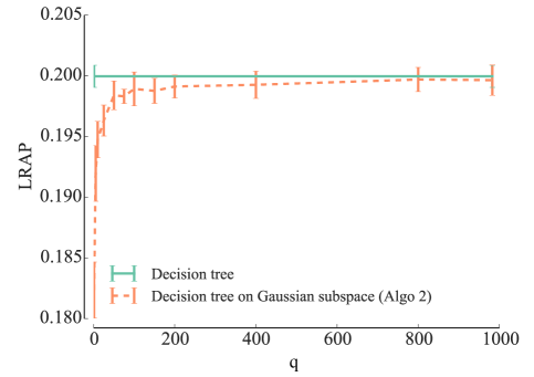
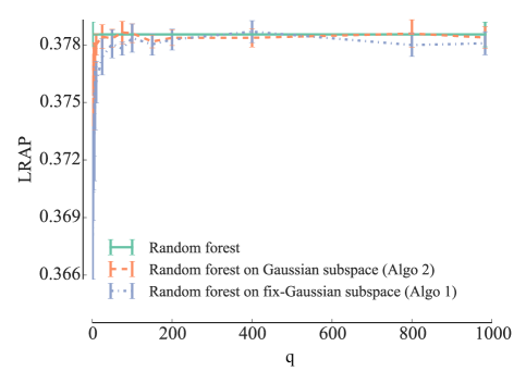
Figure 5.1: Models built for the “Delicious” dataset ($d=983$) for growing numbers $q$ of Gaussian projections. Top: single unpruned CART trees ($n_{\min}=1$); Bottom: Random Forests ($k=\sqrt{p}$, $t=100$, $n_{\min}=1$). The curves represent average values (and standard deviations) obtained from 10 applications of the randomized algorithms over a same single $LS/TS$ split.

To illustrate the behaviour of our algorithms, we first focus on the “Delicious” dataset Tsoumakas et al. (2008a), which has a large number of labels ($d=983$), of input features ($p=500$), and of training ($n_{LS}=12920$) and testing ($n_{TS}=3185$) samples.

The top part of figure 5.1 shows, when Gaussian output-space projections are combined with the standard CART algorithm building a single tree, how the precision converges (cf Theorem 17.12) when $q$ increases towards $d$. We observe that in this case, convergence is reached around $q=200$ at the expense of a slight decrease of accuracy, so that a compression factor of about 5 is possible with respect to the original output dimension $d=983$.

The bottom part of figure 5.1 shows, on the same dataset, how the method behaves when combined with Random Forests. Let us first notice that the Random Forests grown on the original output space (green line) are significantly more accurate than the single trees, their accuracy being almost twice as high. We also observe that Algorithm 2 (orange curve) converges much more rapidly than Algorithm 1 (blue curve) and slightly outperforms the Random Forest grown on the original output space. It needs only about $q=25$ components to converge, while Algorithm 1 needs about $q=75$ of them. These results are in accordance with the analysis of Section 18, showing that Algorithm 2 can’t be inferior to Algorithm 1. In the rest of this chapter we will therefore focus on Algorithm 2.

19.2   Systematic analysis over 24 datasets

To assess our methods, we have collected 24 different multi-label classification datasets from the literature (see Section D of the supplementary material, for more information and bibliographic references to these datasets) covering a broad spectrum of application domains and ranges of the output dimension ($d\in[6;3993]$, see Table 5.1). For 21 of the datasets, we made experiments where the dataset is split randomly into a learning set of size $n_{LS}$, and a test set of size $n_{TS}$, and are repeated 10 times (to get average precisions and standard deviations), and for 3 of them we used a ten-fold cross-validation scheme (see Table 5.1).

Table 5.1 shows our results on the 24 multi-label datasets, by comparing Random Forests learnt on the original output space with those learnt by Algorithm 2 combined with Gaussian subspaces of size $q\in\left\{1,d,\ln{d}\right\}$. In these experiments, the three parameters of Random Forests are set respectively to $k=\sqrt{p}$, $n_{\min}=1$ (default values, see Geurts et al. (2006a)) and $t=100$ (reasonable computing budget). Each model is learnt ten times on a different shuffled train/testing split, except for the 3 EUR-lex datasets where we kept the original 10 folds of cross-validation.

We observe that for all datasets (except maybe SCOP-GO), taking $q=d$ leads to a similar average precision to the standard Random Forests, i.e. no difference superior to one standard deviation of the error. On 11 datasets, we see that $q=1$ already yields a similar average precision (values not underlined in column $q=1$). For the 13 remaining datasets, increasing $q$ to $\ln{d}$ significantly decreases the gap with the Random Forest baseline and 3 more datasets reach this baseline. We also observe that on several datasets such as “Drug-interaction” and “SCOP-GO”, better performance on the Gaussian subspace is attained with high output randomization ($q=\left\{1,\ln{d}\right\}$) than with $q=d$. We thus conclude that the optimal level of output randomization (i.e. the optimal value of the ratio $q/d$) which maximizes accuracy performances, is dataset dependent.

While our method is intended for tasks with very high dimensional output spaces, we however notice that even with relatively small numbers of labels, its accuracy remains comparable to the baseline, with suitable $q$.

Table 5.1: High output space compression ratio is possible, with no or negligible average precision reduction ($t=100$, $n_{\min}=1$, $k=\sqrt{p}$). Each dataset has $n_{LS}$ training samples, $n_{TS}$ testing samples, $p$ input features and $d$ labels. Label ranking average precisions are displayed in terms of their mean values and standard deviations over 10 random $LS/TS$ splits, or over the 10 folds of cross-validation. Mean scores in the last three columns are underlined if they show a difference with respect to the standard Random Forests of more than one standard deviation.

Datasets	Random		Random Forests on Gaussian sub-space
Name	Forests		$q=1$		$q=\lfloor 0.5+\ln{d}\rfloor$		$q=d$
emotions	$0.800$	$\pm 0.014$	$0.800$	$\pm 0.010$	$0.810$	$\pm 0.014$	$0.810$	$\pm 0.016$
scene	$0.870$	$\pm 0.003$	$0.875$	$\pm 0.007$	$0.872$	$\pm 0.004$	$0.872$	$\pm 0.004$
yeast	$0.759$	$\pm 0.008$	$0.748$	$\pm 0.006$	$0.755$	$\pm 0.004$	$0.758$	$\pm 0.005$
tmc2017	$0.756$	$\pm 0.003$	$0.741$	$\pm 0.003$	$0.748$	$\pm 0.003$	$0.757$	$\pm 0.003$
genbase	$0.992$	$\pm 0.004$	$0.994$	$\pm 0.002$	$0.994$	$\pm 0.004$	$0.993$	$\pm 0.004$
reuters	$0.865$	$\pm 0.004$	$0.864$	$\pm 0.003$	$0.863$	$\pm 0.004$	$0.862$	$\pm 0.004$
medical	$0.848$	$\pm 0.009$	$0.836$	$\pm 0.011$	$0.842$	$\pm 0.014$	$0.841$	$\pm 0.009$
enron	$0.683$	$\pm 0.009$	$0.680$	$\pm 0.006$	$0.685$	$\pm 0.009$	$0.686$	$\pm 0.008$
mediamill	$0.779$	$\pm 0.001$	$0.772$	$\pm 0.001$	$0.777$	$\pm 0.002$	$0.779$	$\pm 0.002$
Yeast-GO	$0.420$	$\pm 0.010$	$0.353$	$\pm 0.008$	$0.381$	$\pm 0.005$	$0.420$	$\pm 0.010$
bibtex	$0.566$	$\pm 0.004$	$0.513$	$\pm 0.006$	$0.548$	$\pm 0.007$	$0.564$	$\pm 0.008$
CAL500	$0.504$	$\pm 0.011$	$0.504$	$\pm 0.004$	$0.506$	$\pm 0.007$	$0.502$	$\pm 0.010$
WIPO	$0.490$	$\pm 0.010$	$0.430$	$\pm 0.010$	$0.460$	$\pm 0.010$	$0.480$	$\pm 0.010$
EUR-Lex (subj.)	$0.840$	$\pm 0.005$	$0.814$	$\pm 0.004$	$0.828$	$\pm 0.005$	$0.840$	$\pm 0.004$
bookmarks	$0.453$	$\pm 0.001$	$0.436$	$\pm 0.002$	$0.445$	$\pm 0.002$	$0.453$	$\pm 0.002$
diatoms	$0.700$	$\pm 0.010$	$0.650$	$\pm 0.010$	$0.670$	$\pm 0.010$	$0.710$	$\pm 0.020$
corel5k	$0.303$	$\pm 0.012$	$0.309$	$\pm 0.011$	$0.307$	$\pm 0.011$	$0.299$	$\pm 0.013$
EUR-Lex (dir.)	$0.814$	$\pm 0.006$	$0.782$	$\pm 0.008$	$0.796$	$\pm 0.009$	$0.813$	$\pm 0.007$
SCOP-GO	$0.811$	$\pm 0.004$	$0.808$	$\pm 0.005$	$0.811$	$\pm 0.004$	$0.806$	$\pm 0.004$
delicious	$0.384$	$\pm 0.004$	$0.381$	$\pm 0.003$	$0.382$	$\pm 0.002$	$0.383$	$\pm 0.004$
drug-interaction	$0.379$	$\pm 0.014$	$0.384$	$\pm 0.009$	$0.378$	$\pm 0.013$	$0.367$	$\pm 0.016$
protein-interaction	$0.330$	$\pm 0.015$	$0.337$	$\pm 0.016$	$0.337$	$\pm 0.017$	$0.335$	$\pm 0.014$
Expression-GO	$0.235$	$\pm 0.005$	$0.211$	$\pm 0.005$	$0.219$	$\pm 0.005$	$0.232$	$\pm 0.005$
EUR-Lex (desc.)	$0.523$	$\pm 0.008$	$0.485$	$\pm 0.008$	$0.497$	$\pm 0.009$	$0.523$	$\pm 0.007$

To complete the analysis, let’s carry out the same experiments with a different base-learner combining Gaussian random projections (with $q\in\{1,\ln{d},d\}$) with the Extra Trees method of Geurts et al. (2006a). Results on 23 datasets are compiled in Table 5.2.

Like for Random Forests, we observe that for all 23 datasets taking $q=d$ leads to a similar average precision to the standard Random Forests, ie. no difference superior to one standard deviation of the error. This is already the case with $q=1$ for 12 datasets and with $q=\ln{d}$ for 4 more datasets. Interestingly, on 3 datasets with $q=1$ and 3 datasets with $q=\ln{d}$, the increased randomization brought by the projections actually improves average precision with respect to standard Random Forests (bold values in Table 5.2).

Table 5.2: Experiments with Gaussian projections and Extra Trees (($t=100$, $n_{\min}=1$, $k=\sqrt{p}$). Mean scores in the last three columns are underlined if they show a negative difference with respect to the standard Random Forests of more than one standard deviation. Bold values highlight improvement over standard RF of more than one standard deviation.

Datasets	Extra trees		Extra trees on Gaussian sub-space
			$q=1$		$q=\lfloor 0.5+\ln{d}\rfloor$		$q=d$
emotions	$0.81$	$\pm 0.01$	$0.81$	$\pm 0.014$	$0.80$	$\pm 0.013$	$0.81$	$\pm 0.014$
scene	$0.873$	$\pm 0.004$	$0.876$	$\pm 0.003$	$0.877$	$\pm 0.007$	$0.878$	$\pm 0.006$
yeast	$0.757$	$\pm 0.008$	$0.746$	$\pm 0.004$	$0.752$	$\pm 0.009$	$0.757$	$\pm 0.01$
tmc2017	$0.782$	$\pm 0.003$	$0.759$	$\pm 0.004$	$0.77$	$\pm 0.002$	$0.779$	$\pm 0.002$
genbase	$0.987$	$\pm 0.005$	$0.991$	$\pm 0.004$	$0.992$	$\pm 0.001$	$0.992$	$\pm 0.005$
reuters	$0.88$	$\pm 0.003$	$0.88$	$\pm 0.003$	$0.878$	$\pm 0.004$	$0.88$	$\pm 0.004$
medical	$0.855$	$\pm 0.008$	$\mathbf{0.867}$	$\pm 0.009$	$\mathbf{0.872}$	$\pm 0.006$	$0.862$	$\pm 0.008$
enron	$0.66$	$\pm 0.01$	$0.65$	$\pm 0.01$	$0.663$	$\pm 0.008$	$0.66$	$\pm 0.01$
mediamill	$0.786$	$\pm 0.002$	$0.778$	$\pm 0.002$	$0.781$	$\pm 0.002$	$0.784$	$\pm 0.001$
Yeast-GO	$0.49$	$\pm 0.009$	$0.47$	$\pm 0.01$	$0.482$	$\pm 0.008$	$0.48$	$\pm 0.01$
bibtex	$0.584$	$\pm 0.005$	$0.538$	$\pm 0.005$	$0.564$	$\pm 0.004$	$0.583$	$\pm 0.004$
CAL500	$0.5$	$\pm 0.007$	$0.502$	$\pm 0.008$	$0.499$	$\pm 0.007$	$0.503$	$\pm 0.009$
WIPO	$0.52$	$\pm 0.01$	$0.474$	$\pm 0.007$	$0.49$	$\pm 0.01$	$0.515$	$\pm 0.006$
EUR-Lex (subj.)	$0.845$	$\pm 0.006$	$0.834$	$\pm 0.004$	$0.838$	$\pm 0.003$	$0.845$	$\pm 0.005$
bookmarks	$0.453$	$\pm 0.002$	$0.436$	$\pm 0.002$	$0.444$	$\pm 0.003$	$0.452$	$\pm 0.002$
diatoms	$0.73$	$\pm 0.01$	$0.69$	$\pm 0.01$	$0.71$	$\pm 0.01$	$0.73$	$\pm 0.01$
corel5k	$0.285$	$\pm 0.009$	$\mathbf{0.313}$	$\pm 0.011$	$\mathbf{0.309}$	$\pm 0.009$	$0.285$	$\pm 0.011$
EUR-Lex (dir.)	$0.815$	$\pm 0.007$	$0.805$	$\pm 0.006$	$0.807$	$\pm 0.009$	$0.815$	$\pm 0.007$
SCOP-GO	$0.778$	$\pm 0.005$	$0.782$	$\pm 0.004$	$0.782$	$\pm 0.006$	$0.778$	$\pm 0.005$
delicious	$0.354$	$\pm 0.003$	$\mathbf{0.36}$	$\pm 0.004$	$\mathbf{0.358}$	$\pm 0.004$	$0.355$	$\pm 0.003$
drug-interaction	$0.353$	$\pm 0.011$	$\mathbf{0.375}$	$\pm 0.017$	$0.364$	$\pm 0.014$	$0.355$	$\pm 0.016$
protein-interaction	$0.299$	$\pm 0.013$	$0.307$	$\pm 0.009$	$0.305$	$\pm 0.012$	$0.306$	$\pm 0.017$
Expression-GO	$0.231$	$\pm 0.007$	$0.218$	$\pm 0.005$	$0.228$	$\pm 0.005$	$0.235$	$\pm 0.005$

19.3   Input vs output space randomization

We study in this section the interaction of the additional randomization of the output space with that concerning the input space already built in the Random Forest method.

To this end, we consider the “Drug-interaction” dataset ($p=660$ input features and $d=1554$ output labels Yamanishi et al. (2011)), and we study the effect of parameter $k$ controlling the input space randomization of the Random Forest method with the randomization of the output space by Gaussian projections controlled by the parameter $q$. To this end, Figure 5.2 shows the evolution of the accuracy for growing values of $k$ (i.e. decreasing strength of the input space randomization), for three different quite low values of $q$ (in this case $q\in\left\{1,\ln{d},2\ln{d}\right\}$). We observe that Random Forests learned on a very low-dimensional Gaussian subspace (red, blue and pink curves) yield essentially better performances than Random Forests on the original output space, and also that their behaviour with respect to the parameter $k$ is quite different. On this dataset, the output-space randomisation makes the method completely immune to the ‘over-fitting’ phenomenon observed for high values of $k$ with the baseline method (green curve).

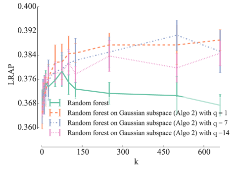
Figure 5.2: Output randomization with Gaussian projections yield better average precision than the original output space on the “Drug-Interaction” dataset ($n_{\min}=1$ , $t=100$).

We carry out the same experiment, but on the “Delicious” dataset. Figure 5.3 shows the evolution of the accuracy for growing values of $k$ (i.e. decreasing strength of the input space randomization), for three different values of $q$ (in this case $q\in\left\{1,\ln{d},2\ln{d}\right\}$) on a Gaussian output space.

Like on “Drug-interaction” (see Figure 5.2), using low-dimensional output spaces makes the method more robust with respect to over-fitting as $k$ increases. However, unlike on “Drug-interaction”, it is not really possible to improve over baseline Random Forests by tuning jointly input and output randomization. This shows that the interaction between $q$ and $k$ may be different from one dataset to another.

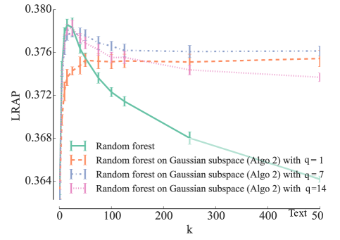
Figure 5.3: “Delicious” dataset: $n_{\min}=1$; $t=100$.

It is thus advisable to jointly optimize the value of $q$ and $k$, so as to maximise the tradeoff between accuracy and computing times in a problem and algorithm specific way.

19.4   Alternative output dimension reduction techniques

In this section, we study Algorithm 2 when it is combined with alternative output-space dimensionality reduction techniques. We focus again on the “Delicious” dataset, but similar trends could be observed on other datasets.

Figure 5.4a first compares Gaussian random projections with two other dense projections: Rademacher matrices with $s=1$ (cf. Section 2.2) and compression matrices obtained by sub-sampling (without replacement) Hadamard matrices Candes and Plan (2011). We observe that Rademacher and subsample-Hadamard sub-spaces behave very similarly to Gaussian random projections.

In a second step, we compare Gaussian random projections with two (very) sparse projections: first, sparse Rademacher sub-spaces obtained by setting the sparsity parameter $s$ to $3$ and $\sqrt{d}$, selecting respectively about 33% and 2% of the original outputs to compute each component, and second, sub-sampled identity subspaces, similar to Tsoumakas and Vlahavas (2007), where each of the $q$ selected components corresponds to a randomly chosen original label and also preserve sparsity. Sparse projections are very interesting from a computational point of view as they require much less operations to compute the projections but the number of components required for condition (2.86) to be satisfied is typically higher than for dense projections Li et al. (2006); Candes and Plan (2011). Figure 5.4b compares these three projection methods with standard Random Forests on the “delicious” dataset. All three projection methods converge to plain Random Forests as the number of components $q$ increases but their behaviour at low $q$ values are very different. Rademacher projections converge faster with $s=3$ than with $s=1$ and interestingly, the sparsest variant ($s=\sqrt{d}$) has its optimum at $q=1$ and improves in this case over the Random Forests baseline. Random output subspaces converge slower but they lead to a notable improvement of the score over baseline Random Forests. This suggests that although their theoretical guarantees are less good, sparse projections actually provide on this problem a better bias/variance tradeoff than dense ones when used in the context of Algorithm 2.

Another popular dimension reduction technique is the principal component analysis (PCA). In Figure 5.4c, we repeat the same experiment to compare PCA with Gaussian random projections. Concerning PCA, the curve is generated in decreasing order of eigenvalues, according to their contribution to the explanation of the output-space variance. We observe that this way of doing is far less effective than the random projection techniques studied previously.

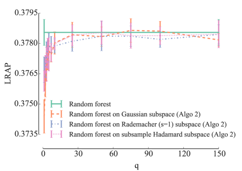
(a) Computing the impurity criterion on a dense Rademacher or on a subsample-Hadamard output sub-space is another efficient way to learn tree ensembles.

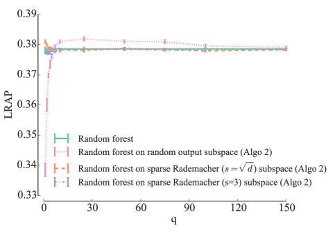
(b) Sparse random projections output sub-space yield better average precision than on the original output space.

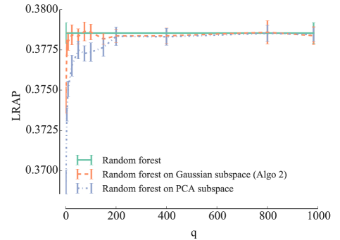
(c) PCA compared with Gaussian subspaces.

Figure 5.4: “Delicious” dataset, $t=100$, $k=\sqrt{p}$, $n_{\min}=1$.

19.5   Learning stage computing times

Our implementation of the learning algorithms is based on the scikit-learn Python package version 0.14-dev Pedregosa et al. (2011); Buitinck et al. (2013). To fix ideas about computing times, we report these obtained on a Mac Pro 4.1 with a dual Quad-Core Intel Xeon processor at 2.26 GHz, on the “Delicious” dataset. Matrix operation, such as random projections, are performed with the BLAS and the LAPACK from the Mac OS X Accelerate framework. Reported times are obtained by summing the user and sys time of the UNIX time utility.

The reported timings correspond to the following operation: (i) load the dataset in memory, (ii) execute the algorithm. All methods use the same code to build trees. In these conditions, learning a random forest on the original output space ($t=100$, $n_{\min}=1$, $k=\sqrt{d}$) takes 3348  s; learning the same model on a Gaussian output space of size $q=25$ requires 311 s, while $q=1$ and $q=250$ take respectively 236 s and 1088 s. Generating a Gaussian sub-space of size $q=25$ and projecting the output data of the training samples is done in less than 0.25 s, while $q=1$ and $q=250$ takes around 0.07 s and 1 s respectively. The time needed to compute the projections is thus negligible with respect to the time needed for the tree construction.

We see that a speed-up of an order of magnitude could be obtained, while at the same time preserving accuracy with respect to the baseline Random Forests method. Equivalently, for a fixed computing time budget, randomly projecting the output space allows to build more trees and thus to improve predictive performances with respect to standard Random Forests.

20   Conclusions

This chapter explores the use of random output space projections combined with tree-based ensemble methods to address large-scale multi-label classification problems. We study two algorithmic variants that either build a tree-based ensemble model on a single shared random subspace or build each tree in the ensemble on a newly drawn random subspace. The second approach is shown theoretically and empirically to always outperform the first in terms of accuracy. Experiments on 24 datasets show that on most problems, using gaussian projections allows to reduce very drastically the size of the output space, and therefore computing times, without affecting accuracy. Remarkably, we also show that by adjusting jointly the level of input and output randomizations and choosing appropriately the projection method, one could also improve predictive performance over the standard Random Forests, while still improving very significantly computing times. As future work, it would be very interesting to propose efficient techniques to automatically adjust these parameters, so as to reach the best tradeoff between accuracy and computing times on a given problem.

To the best of our knowledge, our work is the first to study random output projections in the context of multi-output tree-based ensemble methods. The possibility with these methods to relabel tree leaves with predictions in the original output space makes this combination very attractive. Indeed, unlike similar works with linear models Hsu et al. (2009); Cisse et al. (2013), our approach only relies on Johnson-Lindenstrauss lemma, and not on any output sparsity assumption, and also does not require to use any output reconstruction method. Besides multi-label classification, we would like to test our method on other, not necessarily sparse, multi-output prediction problems.

Gradient boosting with random output projections for multi-label and multi-outputs regression tasks

Remark 20.14.

Outline We first formally adapt the gradient boosting ensemble method for multi-output supervised learning tasks such as multi-output regression and multi-label classification. We then propose to combine single random projections of the output space with gradient boosting on such tasks to adapt automatically to the output correlation structure. The idea of this method is to train each weak model on a single random projection of the output space and then to exploit the predictions of the resulting model to approximate the gradients of all other outputs. Through weak model sharing and random projection of the output space, we implicitly take into account the output correlations. We perform extensive experiments with these methods both on artificial and real problems using tree-based weak learners. Randomly projecting the output space shows to provide a better adaptation to different output correlation patterns and is therefore competitive with the best of the other methods in most settings. Thanks to the model sharing, the convergence speed is also faster, reducing the computing times to reach a specific accuracy.

This contribution is a joint work with Pierre Geurts and Louis Wehenkel from the University of Liège.

21   Introduction

Multi-output supervised learning aims to model the input-output relationship of a system from observations of input-output pairs whenever the output space is a vector of random variables. Multi-output classification and regression tasks have numerous applications in domains ranging from biology to multimedia.

The most straightforward way to address multi-output tasks is to apply standard single output methods separately and independently on each output. Although simple, this method, called binary relevance Tsoumakas et al. (2009) in multi-label classification or single target Spyromitros-Xioufis et al. (2016) in multi-output regression, is often suboptimal as it does not exploit potential correlations that might exist between the outputs. For this reason, several approaches have been proposed in the literature that improve over binary relevance by exploiting output correlations. These approaches include for example the explicit construction of the output dependency graph Dembczynski et al. (2010); Gasse et al. (2015); Zhang and Zhang (2010) or the sharing of models learnt for one output to the other outputs Huang et al. (2012); Yan et al. (2007); Read et al. (2011). Our contribution falls into the latter category.

Classification and regression trees Breiman et al. (1984) are popular supervised learning methods that provide state-of-the-art accuracy when exploited in the context of ensemble methods, namely Random forests Breiman (2001) and gradient boosting Friedman (2001). Classification and regression trees have been extended by several authors to the joint prediction of multiple outputs (see, e.g., Segal, 1992; Blockeel et al., 2000)). These extensions build a single tree to predict all outputs at once. They adapt the score measure used to assess splits during the tree growth to take into account all outputs and label each tree leaf with a vector of values, one for each output (see Section 13 for more information). Like standard classification or regression trees, multiple output trees can be exploited in the context of random forests Barutcuoglu et al. (2006); Joly et al. (2014); Kocev et al. (2007, 2013); Segal and Xiao (2011) or boosting Geurts et al. (2007) ensembles, which often offer very significant accuracy improvements with respect to single trees. Multiple output trees have been shown to be competitive with other multiple output methods Madjarov et al. (2012), but, to the best of our knowledge, it has not been studied as extensively in the context of gradient boosting.

Binary relevance / single target of single output tree models and multiple output tree models represent two extremes in terms of tree structure learning: the former builds a separate tree ensemble structure for each output, while the latter builds a single tree ensemble structure for all outputs. Building separate ensembles for each output may be rather inefficient when the outputs are strongly correlated. Correlations between the outputs could indeed be exploited either to reduce model complexity (by sharing the tree structures between several outputs) or to improve accuracy by regularization. Trying to fit a single tree structure for all outputs seems however counterproductive when the outputs are independent. Indeed, in the case of independent outputs, simultaneously fitting all outputs with a single tree structure may require a much more complex tree structure than the sum of the individual tree complexities required to fit the individual outputs. Since training a more complex tree requires a larger learning sample, multiple output trees are expected to be outperformed by binary relevance / single target in this situation.

In this chapter, we first formally adapt gradient boosting to multiple output tasks. We then propose a new method that aims at circumventing the limitations of both binary relevance / single target and multiple output methods, in the specific context of tree-based base-learners. Our method is an extension of gradient tree boosting that can adapt itself to the presence or absence of correlations between the outputs. At each boosting iteration, a single regression tree structure is grown to fit a single random projection of the outputs, or more precisely, of their residuals with respect to the previously built models. Then, the predictions of this tree are fitted linearly to the current residuals of all the outputs (independently). New residuals are then computed taking into account the resulting predictions and the process repeats itself to fit these new residuals. Because of the linear fit, only the outputs that are correlated with the random projection at each iteration will benefit from a reduction of their residuals, while outputs that are independent of the random projection will remain mostly unaffected. As a consequence, tree structures will only be shared between correlated outputs as one would expect. Another variant that we explore consists in replacing the linear global fit by a relabelling of all tree leaves for each output in turn.

The chapter is structured as follows. We show how to extend the gradient boosting algorithms to multi-output tasks in Section 22. We provide for these algorithms a convergence proof on the training data and discuss the effect of the random projection of the output space. We study empirically the proposed approach in Section 23. Our first experiments compare the proposed approaches to binary relevance / single target on artificial datasets where the output correlation is known. We also highlight the effect of the choice and size of the random projection space. We finally carry out an empirical evaluation of these methods on 21 real-world multi-label and 8 multi-output regression tasks. We draw our conclusions in Section 24.

22   Gradient boosting with multiple outputs

Starting from a multi-output loss, we show in Section 22.1 how to extend the standard gradient boosting algorithm to solve multi-output tasks, such as multi-output regression and multi-label classification, by exploiting existing weak model learners suited for multi-output prediction. In Section 22.2, we then propose to combine single random projections of the output space with gradient boosting to automatically adapt to the output correlation structure on these tasks. We discuss and compare the effect of the random projection of the output space in Section 22.3. We give a convergence proof on the training data for the proposed algorithms in Section 22.4.

22.1   Standard extension of gradient boosting to multi-output tasks

A loss function $\ell(y,y^{\prime})\in\mathbb{R}^{+}$ computes the difference between a ground truth $y$ and a model prediction $y^{\prime}$. It compares scalars with single output tasks and vectors with multi-output tasks. The two most common regression losses are the square loss $\ell_{square}(y,y^{\prime})=\frac{1}{2}(y-y^{\prime})^{2}$ and the absolute loss $\ell_{absolute}(y,y)=|y-y^{\prime}|$. Their multi-output extensions are the $\ell_{2}$-norm and $\ell_{1}$-norm losses:

$$\ell_{2}(y,y^{\prime}) =\frac{1}{2}||y-y^{\prime}||_{\ell_{2}}^{2},$$ (6.1)

$$\ell_{1}(y,y^{\prime}) =||y-y^{\prime}||_{\ell_{1}}.$$ (6.2)

In classification, the most commonly used loss to compare a ground truth $y$ to the model prediction $f(x)$ is the $0-1$ loss $\ell_{0-1}(y,y^{\prime})=1(y\not=y^{\prime})$, where $1$ is the indicator function. It has two standard multiple output extensions (i) the Hamming loss $\ell_{Hamming}$ and (ii) the subset $0-1$ loss $\ell_{\text{subset }0-1}$:

$$\ell_{Hamming}(y,y^{\prime}) =\sum_{j=1}^{d}1(y_{j}\not=y^{\prime}_{j}),$$ (6.3)

$$\ell_{\text{subset }0-1}(y,y^{\prime}) =1(y\not=y^{\prime}).$$ (6.4)

Since these losses are discrete, they are non-differentiable and difficult to optimize. Instead, we propose to extend the logistic loss $\ell_{logistic}(y,y^{\prime})=\log(1+\exp(-2yy^{\prime}))$ used for binary classification tasks to the multi-label case, as follows:

$$\ell_{logistic}(y,y^{\prime})=\sum_{j=1}^{d}\log(1+\exp(-2y_{j}y^{\prime}_{j})),$$ (6.5)

where we suppose that the $d$ components $y_{j}$ of the target output vector belong to $\{-1,1\}$, while the $d$ components $y^{\prime}_{j}$ of the predictions may belong to $\mathbb{R}$.

Given a training set $\mathcal{L}=\left((x^{i},y^{i})\in\mathcal{X}\times\mathcal{Y}\right)_{i=1}^{n}$ and one of these multi-output losses $\ell$, we want to learn a model $f_{M}$ expressed in the following form

$$f_{M}(x)=\rho_{0}+\sum_{m=1}^{M}\rho_{m}\odot g_{m}(x),$$ (6.6)

where the terms $g_{m}$ are selected within a hypothesis space $\mathcal{H}$ of weak multi-output base-learners, the coefficients $\{\rho_{m}\in\mathbb{R}^{d}\}_{m=0}^{M}$ are $d$-dimensional vectors highlighting the contributions of each term $g_{m}$ to the ensemble, and where the symbol $\odot$ denotes the Hadamard product. Note that the prediction $f_{M}(x)\in\mathbb{R}^{d}$ targets the minimization of the chosen loss $\ell$, but a transformation might be needed to have a prediction in $\mathcal{Y}$, e.g. we would apply the $\operatorname{logit}$ function to each output for the multi-output logistic loss to get a probability estimate of the positive classes.

The gradient boosting method builds such a model in an iterative fashion, as described in Algorithm 1, and discussed below.

Algorithm 1 Gradient boosting with multi-output regressor weak models.

1:function GB-mo($\mathcal{L}=\left((x^{i},y^{i})\right)_{i=1}^{n};\ell;\mathcal{H};M$)

2:     $f_{0}(x)=\rho_{0}=\arg\min_{\rho\in\mathbb{R}^{d}}\sum_{i=1}^{n}\ell(y^{i},\rho)$

3:     for $m$ = 1 to $M$ do

4:         Compute the loss gradient for the learning set samples

$$g_{m}^{i}\in\mathbb{R}^{d}=\left[\nabla_{y^{\prime}}\ell(y^{i},y^{\prime})\right]_{y^{\prime}=f_{m-1}(x^{i})}\forall i\in\left\{1,\ldots,n\right\}.$$

5:         Fit the negative loss gradient

$$g_{m}=\arg\min_{g\in\mathcal{H}}\sum_{i=1}^{n}\left|\left|-g_{m}^{i}-g(x^{i})\right|\right|_{\ell_{2}}^{2}.$$

6:         Find an optimal step length in the direction of $g_{m}$

$$\rho_{m}=\arg\min_{\rho\in\mathbb{R}^{d}}\sum_{i=1}^{n}\ell\left(y^{i},f_{m-1}(x^{i})+\rho\odot g_{m}(x^{i})\right).$$

7:         $f_{m}(x)=f_{m-1}(x)+\rho_{m}\odot g_{m}(x)$

8:     end for

9:     return $f_{M}(x)$

10:end function

To build the ensemble model, we first initialize it with the constant model defined by the vector $\rho_{0}\in\mathbb{R}^{d}$ minimizing the multi-output loss $\ell$ (line 2):

$$\rho_{0}=\arg\min_{\rho\in\mathbb{R}^{d}}\sum_{i=1}^{n}\ell(y^{i},\rho).$$ (6.7)

At each subsequent iteration $m$, the multi-output gradient boosting approach adds a new multi-output weak model $g_{m}(x)$ with a weight $\rho_{m}$ to the current ensemble model by approximating the minimization of the multi-output loss $\ell$:

$$(\rho_{m},g_{m})=\arg{}\min_{(\rho,g)\in\mathbb{R}^{d}\times\mathcal{H}}\sum_{i=1}^{n}\ell\left(y^{i},f_{m-1}(x^{i})+\rho\odot g(x^{i})\right).$$ (6.8)

To approximate Equation 6.8, it first fits a multi-output weak model $g_{m}$ to model the negative gradient $g_{m}^{i}$ of the multi-output loss $\ell$

$$g_{m}^{i}\in\mathbb{R}^{d}=\left[\nabla_{y^{\prime}}\ell(y^{i},y^{\prime})\right]_{y^{\prime}=f_{m-1}(x^{i})}$$ (6.9)

associated to each sample $i\in\mathcal{L}$ of the training set, by minimizing the $\ell_{2}$-loss:

$$g_{m}=\arg\min_{{g}\in\mathcal{H}}\sum_{i=1}^{n}\left|\left|-g_{m}^{i}-{g}(x^{i})\right|\right|_{\ell_{2}}^{2}.$$ (6.10)

It then computes an optimal step length vector $\rho_{m}\in\mathbb{R}^{d}$ in the direction of the weak model $g_{m}$ to minimize the multi-output loss $\ell$:

$$\rho_{m}=\arg\min_{\rho\in\mathbb{R}^{d}}\sum_{i=1}^{n}\ell\left(y^{i},f_{m-1}(x^{i})+\rho\odot g_{m}(x^{i})\right).$$ (6.11)

22.2   Adapting to the correlation structure in the output-space

Binary relevance / single target of gradient boosting models and gradient boosting of multi-output models (Algorithm 1) implicitly target two extreme correlation structures. On the one hand, binary relevance / single target predicts all outputs independently, thus assuming that outputs are not correlated. On the other hand, gradient boosting of multi-output models handles them all together, thus assuming that they are all correlated. Both approaches thus exploit the available dataset in a rather biased way. To remove this bias, we propose a more flexible approach that can adapt itself automatically to the correlation structure among output variables.

Our idea is that a weak learner used at some step of the gradient boosting algorithm could be fitted on a single random projection of the output space, rather than always targeting simultaneously all outputs or always targeting a single a priori fixed output.

We thus propose to first generate at each iteration of the boosting algorithm one random projection vector of size $\phi_{m}\in\mathbb{R}^{1\times d}$. The weak learner is then fitted on the projection of the current residuals according to $\phi_{m}$ reducing dimensionality from $d$ outputs to a single output. A weight vector $\rho_{m}\in\mathbb{R}^{d}$ is then selected to minimize the multi-output loss $\ell$. The whole approach is described in Algorithm 2. If the loss is decomposable, non zero components of the weight vector $\rho_{m}$ highlight the contribution of the current $m$-th model to the overall loss decrease. Note that sign flips due to the projection are taken into account by the additive weights $\rho_{m}$. A single output regressor can now handle multi-output tasks through a sequence of single random projections.

The prediction of an unseen sample $x$ by the model produced by Algorithm 2 is now given by

$$f(x)=\rho_{0}+\sum_{m=1}^{M}\rho_{m}g_{m}(x),$$ (6.12)

where $\rho_{0}\in\mathbb{R}^{d}$ is a constant prediction, and the coefficients $\{\rho_{m}\in\mathbb{R}^{d}\}_{m=1}^{M}$ highlight the contribution of each model $g_{m}$ to the ensemble. Note that it is different from Equation 6.6 (no Hadamard product), since here the weak models $g_{m}$ produce single output predictions.

Algorithm 2 Gradient boosting on randomly projected residual spaces.

1:function GB-rpo($\mathcal{L}=\left((x^{i},y^{i})\right)_{i=1}^{n};\ell;\mathcal{H};M$)

2:     $f_{0}(x)=\rho_{0}=\arg\min_{\rho\in\mathbb{R}^{d}}\sum_{i=1}^{n}\ell(y^{i},\rho)$

3:     for $m$ = 1 to $M$ do

4:         Compute the loss gradient for the learning set samples

$$g_{m}^{i}\in\mathbb{R}^{d}=\left[\nabla_{y^{\prime}}\ell(y^{i},y^{\prime})\right]_{y^{\prime}=f_{m-1}(x^{i})}\forall i\in\left\{1,\ldots,n\right\}.$$

5:         Generate a random projection $\phi_{m}\in\mathbb{R}^{1\times d}$.

6:         Fit the projected loss gradient

$$g_{m}=\arg\min_{{g}\in\mathcal{H}}\sum_{i=1}^{n}\left(-\phi_{m}g_{m}^{i}-{g}(x^{i})\right)^{2}.$$

7:         Find an optimal step length in the direction of $g_{m}$.

$$\rho_{m}=\arg\min_{\rho\in\mathbb{R}^{d}}\sum_{i=1}^{n}\ell\left(y^{i},f_{m-1}(x^{i})+\rho g_{m}(x^{i})\right),$$

8:         $f_{m}(x)=f_{m-1}(x)+\rho_{m}g_{m}(x)$

9:     end for

10:     return $f_{M}(x)$

11:end function

Whenever we use decision trees as models, we can grow the tree structure on any output space and then (re)label it in another one as in Chapter 5 Section 17.1 by (re)propagating the training samples in the tree structure. This idea of leaf relabelling could be readily applied to Algorithm 2 leading to Algorithm 3. After fitting the decision tree on the random projection(s) and before optimizing the additive weights $\rho_{m}$, we relabel the tree structure in the original residual space (line 7). More precisely, each leaf is labelled by the average unprojected residual vector of all training examples falling into that leaf. The predition of an unseen sample is then obtained with Equation 6.6 as for Algorithm 1. We will investigate whether it is better or not to relabel the decision tree structure in the experimental section. Note that Algorithm 3 can be straightforwardly used in a multiple random projection context ($q\geq 1$) using a random projection matrix $\phi_{m}\in\mathcal{R}^{q\times d}$. The resulting algorithm with arbitrary $q$ corresponds to the application to gradient boosting of the idea explored in Chapter 5 in the context of random forests. We will study in Section 22.3.3 and Section 23.3.2 the effect of the size of the projected space $q$.

Algorithm 3 Gradient boosting on randomly projected residual spaces with relabelled decision trees as weak models.

1:function GB-relabel-rpo($\mathcal{L}=\left((x^{i},y^{i})\right)_{i=1}^{n};\ell;\mathcal{H};M;q$)

2:     $f_{0}(x)=\rho_{0}=\arg\min_{\rho\in\mathbb{R}^{d}}\sum_{i=1}^{n}\ell(y^{i},\rho)$

3:     for $m$ = 1 to $M$ do

4:          Compute the loss gradient for the learning set samples $$g_{m}^{i}\in\mathbb{R}^{d}=\left[\nabla_{y^{\prime}}\ell(y^{i},y^{\prime})\right]_{y^{\prime}=f_{m-1}(x^{i})}\forall i\in\left\{1,\ldots,n\right\}.$$

5:          Generate a random projection $\phi_{m}\in\mathbb{R}^{q\times d}$.

6:          Fit a single-output tree $g_{m}$ on the projected negative loss gradients $$g_{m}=\arg\min_{g\in\mathcal{H}}\sum_{i=1}^{n}\left|\left|-\phi_{m}g_{m}^{i}-{g}(x^{i})\right|\right|_{\ell_{2}}^{2}.$$

7:          Relabel each leaf of the tree $g_{m}$ in the original (unprojected) residual space, by averaging at each leaf the $g_{m}^{i}$ vectors of all examples falling into that leaf.

8:          Find an optimal step length in the direction of $g^{\prime}_{m}$.

$$\rho_{m}=\arg\min_{\rho\in\mathbb{R}^{d}}\sum_{i=1}^{n}\ell\left(y^{i},f_{m-1}(x^{i})+\rho\odot g^{\prime}_{m}(x^{i})\right).$$

9:          $f_{m}(x)=f_{m-1}(x)+\rho_{m}\odot g^{\prime}_{m}(x)$

10:     end for

11:     return $f_{M}(x)$

12:end function

To the three presented algorithms, we also add a constant learning rate $\mu\in(0,1]$ to shrink the size of the gradient step $\rho_{m}$ in the residual space. Indeed, for a given weak model space $\mathcal{H}$ and a loss $\ell$, optimizing both the learning rate $\mu$ and the number of steps $M$ typically improves generalization performance.

22.3   Effect of random projections

Randomly projecting the output space in the context of the gradient boosting approach has two direct consequences: (i) it strongly reduces the size of the output space, and (ii) it randomly combines several outputs. We will consider here the following random projection matrices $\phi\in\mathbb{R}^{q\times d}$ ordered from the sparsest to the densest ones:

• Random output subsampling matrices is obtained by sampling random lines from the identity matrix.

• (Sparse) Rademacher matrices is obtained by drawing its elements in $\left\{-\sqrt{\frac{s}{q}},0,\sqrt{\frac{s}{q}}\right\}$ with probability $\left\{\frac{1}{2s},1-\frac{1}{s},\frac{1}{2s}\right\}$, where $1/s\in(0,1]$ controls the sparsity of $\phi$. With $s=1$, we have (dense) Rademacher random projections. If $s=3$, we will call them Achlioptas random projections Achlioptas (2003). When $s=\sqrt{d}$, we will say that we have sparse random projections as in Li et al. (2006).

• Gaussian matrices are obtained by drawing their elements i.i.d. in $\mathcal{N}(0,1/q)$.

We discuss in more details the random sub-sampling projection in Section 22.3.1 and the impact of the density of random projection matrices in Section 22.3.2. We study the benefit to use more than a single random projection of the output space ($q>1$) in Section 22.3.3. We highlight the difference in model representations between tree ensemble techniques, i.e. the gradient tree boosting approaches and the random forest approaches, in Section 22.3.4.

22.3.1   $\ell_{2}$-norm loss and random output sub-sampling

The gradient boosting method has an analytical solution when the loss is the square loss or its extension the $\ell_{2}$-norm loss $\ell_{2}(y,y^{\prime})=\frac{1}{2}||y-y^{\prime}||^{2}$:

• The constant model $f_{0}$ minimizing this loss is the average output value of the training set given by

  $$f_{0}(x)=\rho_{0}=\arg\min_{\rho\in\mathbb{R}^{d}}\sum_{i=1}^{n}\frac{1}{2}||y^{i}-\rho||_{\ell_{2}}^{2}=\frac{1}{n}\sum_{i=1}^{n}y^{i}.$$ (6.13)

• The gradient of the $\ell_{2}$-norm loss for the $i$-th sample is the difference between the ground truth $y^{i}$ and the prediction of the ensemble $f$ at the current step $m$ ($\forall i\in\left\{1,\ldots,n\right\}$):

  $$g_{m}^{i} =\left[\nabla_{y^{\prime}}\ell(y^{i},y^{\prime})\right]_{y^{\prime}=f_{m-1}(x^{i})}=y^{i}-f_{m-1}(x^{i}).$$ (6.14)

• Once a new weak estimator $g_{m}$ has been fitted on the loss gradient $g_{m}^{i}$ or the projected gradient $\phi_{m}g_{m}^{i}$ with or without relabelling, we have to optimize the multiplicative weight vector $\rho_{m}$ of the new weak model in the ensemble. For Algorithm 1 and Algorithm 3 that exploit multi-output weak learners, this amounts to

  $$\rho_{m} =\arg\min_{\rho\in\mathbb{R}^{d}}\sum_{i=1}^{n}\frac{1}{2}\left|\left|y^{i}-f_{m}(x^{i})-\rho\odot g_{m}(x^{i})\right|\right|^{2}$$ (6.15)

  $$=\arg\min_{\rho\in\mathbb{R}^{d}}\sum_{i=1}^{n}\frac{1}{2}\left|\left|g_{m}^{i}-\rho\odot g_{m}(x^{i})\right|\right|^{2}$$ (6.16)

  which has the following solution:

  $$\rho_{m,j}=\frac{\sum_{i=1}^{n}g_{m,j}^{i}g_{m}(x^{i})_{j}}{\sum_{i=1}^{n}g_{m}(x^{i})_{j}}\forall j~\in\{1,\ldots,d\}.$$ (6.17)

  For Algorithm 2, we have to solve

  $$\rho_{m} =\arg\min_{\rho\in\mathbb{R}^{d}}\sum_{i=1}^{n}\frac{1}{2}\left|\left|y^{i}-f_{m}(x^{i})-\rho g_{m}(x^{i})\right|\right|^{2}$$ (6.18)

  $$=\arg\min_{\rho\in\mathbb{R}^{d}}\sum_{i=1}^{n}\frac{1}{2}\left|\left|g_{m}^{i}-\rho g_{m}(x^{i})\right|\right|^{2}$$ (6.19)

  which has the following solution

  $$\rho_{m,j}=\frac{\sum_{i=1}^{n}g_{m,j}^{i}g_{m}(x^{i})}{\sum_{i=1}^{n}g_{m}(x^{i})}\forall j~\in\{1,\ldots,d\}.$$ (6.20)

From Equation 6.17 and Equation 6.20, we have that the weight $\rho_{m,j}$ is proportional to the correlation between the loss gradient of the output $j$ and the weak estimator $g_{m}$. If the model $g_{m}$ is independent of the output $j$, the weight $\rho_{m,j}$ will be close to zero and $g_{m}$ will thus not contribute to the prediction of this output. On the opposite, a high magnitude of $|\rho_{m,j}|$ means that the model $g_{m}$ is useful to predict the output $j$.

If we subsample the output space at each boosting iteration (Algorithm 2 with random output sub-sampling), the weight $\rho_{m,j}$ is then proportional to the correlation between the model fitted on the sub-sampled output and the output $j$. If correlations exist between the outputs, the optimization of the constant $\rho_{m}$ allows to share the trained model at the $m$-th iteration on the sub-sampled output to all the other outputs. In the extreme case where all outputs are independent given the inputs, the weight $\rho_{m}$ is expected to be nearly zero for all outputs except for the sub-sampled output, and Algorithm 2 would be equivalent to the binary relevance / single target approach. If all outputs are strictly identical, the elements of the constant vector $\rho_{m}$ would have the same value, and Algorithm 2 would be equivalent to the multi-output gradient boosting approach (Algorithm 1). Algorithm 2 would also produce in this case the exact same model as binary relevance / single target approach asymptotically but it would require $d$ times less trees to reach similar performance, as each tree would be shared by all $d$ outputs.

Algorithm 3 with random output sub-sampling is a gradient boosting approach fitting one decision tree at each iteration on a random output space and relabelling the tree in the original output space. The leaf relabelling procedure minimizes the $\ell_{2}$-norm loss over the training samples by averaging the output values of the samples reaching the corresponding leaves. In this case, the optimization of the weight $\rho_{m}$ is unnecessary, as it would lead to an all ones vector. For similar reasons if the multi-output gradient boosting method (Algorithm 1) uses decision trees as weak estimators, the weight $\rho_{m}$ is also an all ones vector as the leaf predictions already minimize the $\ell_{2}$-norm loss. The difference between these two algorithms is that Algorithm 3 grows trees using a random output at each iteration instead of all of them with Algorithm 1.

22.3.2   Density of the random projections

In Chapter 5, we have combined the random forest method with a wide variety of random projection schemes. While the algorithms presented in this chapter were originally devised with random output sub-sampling in mind (see Section 22.3.1), it seems natural to also combine the proposed approaches with random projection schemes such as Gaussian random projections or (sparse) Rademacher random projections.

With random output sub-sampling, the projection matrix $\phi_{m}\in\mathbb{R}^{1\times d}$ is extremely sparse as only one element is non zero. With denser random projections, the weak estimators of Algorithm 2 and Algorithm 3 are fitted on the projected gradient loss $\{(x^{i},\phi_{m}g_{m}^{i}\}_{i=1}^{n}$. It means that a weak estimator $g_{m}$ is trying to model the direction of a weighted combination of the gradient loss.

Otherwise said, the weak model fitted at the $m$-th step approximates a projection $\phi_{m}$ of the gradient losses given the input vector. We can interpret the weight $\rho_{m,j}$ when minimizing the $\ell_{2}$-norm loss as the correlation between the output $j$ and a weighted approximation of the output variables $\phi_{m}$. With an extremely sparse projection having only one non zero element, we have the situation described in the previous section. If we have two non zero elements, we have the following extreme cases: (i) both combined outputs are identical and (ii) both combined outputs are independent given the inputs. In the first situation, the effect is identical to the case where we sub-sample only one output. In the second situation, the weak model makes a compromise between the independent outputs given by $\phi_{m}$. Between those two extremes, the loss gradient direction $\phi_{m}$ approximated by the weak model is useful to predict both outputs. The random projection of the output space will indeed prevent over-fitting by inducing some variance in the learning process. The previous reasoning can be extended to more than two output variables.

Dense random projection schemes, such as Gaussian random projection, consider a higher number of outputs together and is hoped to speed up convergence by increasing the correlation between the fitted tree in the projected space and the residual space. Conversely, sparse random projections, such as random output sub-sampling, make the weak model focus on few outputs.

22.3.3   Gradient tree boosting and multiple random projections

The gradient boosting multi-output strategy combining random projections and tree relabelling (Algorithm 3) can use random projection matrices $\phi_{m}\in\mathbb{R}^{q\times d}$ with more than one line ($q\geq 1$).

The weak estimators are multi-output regression trees using the variance as impurity criterion to grow their tree structures. With an increasing number of projections $q$, we have the theoretical guarantee (see Chapter 5) that the variance computed in the projected space is an approximation of the variance in the original output space.

When the projected space is of infinite size $q\rightarrow\infty$, the decision trees grown on the original space or on the projected space are identical as the approximation of the variance is exact. We thus have that Algorithm 3 is equivalent to the gradient boosting with multi-output regression tree method (Algorithm 1).

Whenever the projected space is of finite size ($q<\infty$), Algorithm 3 is thus an approximation of Algorithm 1. We study empirically the effect of the number of projections $q$ in Algorithm 3 in Section 23.3.2.

22.3.4   Representation bias of decision tree ensembles

Random forests and gradient tree boosting build an ensemble of trees either independently or sequentially, and thus offer different bias/variance tradeoffs. The predictions of all these ensembles can be expressed as a weighted combination of the ground truth outputs of the training set samples. In the present section, we discuss the differences between single tree models, random forest models and gradient tree boosting models in terms of the representation biases of the obtained models. We also highlight the differences between single target models and multi-output tree models.

Single tree models.

The prediction of a regression tree learner can be written as a weighted linear combination of the training samples $\mathcal{L}=\{(x^{i},y^{i})\in\mathcal{X}\times\mathcal{Y}\}_{i=1}^{n}$. We associate to each training sample $(x^{i},y^{i})$ a weight function $w^{i}:\mathcal{X}\rightarrow\mathbb{R}$ which gives the contribution of a ground truth $y^{i}$ to predict an unseen sample $x$. The prediction of a single output tree $f$ is given by

$$f(x)=\sum_{i=1}^{n}w^{i}(x)y^{i}.$$ (6.21)

The weight function $w^{i}(x)$ is non zero if both the samples $(x^{i},y^{i})$ and the unseen sample $x$ reach the same leaf of the tree. If both $(x^{i},y^{i})$ and $x$ end up in the same leaf of the tree, $w^{i}(x)$ is equal to the inverse of the number of training samples reaching that leaf. The weight $w^{i}(x)$ can thus be rewritten as $k(x^{i},x)$ and the function $k(\cdot,\cdot)$ is actually a positive semi-definite kernel Geurts et al. (2006a).

We can also express multi-output models as a weighted sum of the training samples. With a single target regression tree, we have an independent weight function $w^{i}_{j}$ for each sample of the training set and each output as we fit one model per output. The prediction of this model for output $j$ is given by:

$$f(x)_{j}=\sum_{i=1}^{n}w^{i}_{j}(x)y^{i}_{j}.$$ (6.22)

With a multi-output regression tree, the decision tree structure is shared between all outputs so we have a single weight function $w^{i}$ for each training sample:

$$f(x)_{j}=\sum_{i=1}^{n}w^{i}(x)y^{i}_{j}.$$ (6.23)

Random forest models.

If we have a single target random forest model, the prediction of the $j$-th output combines the predictions of the $M$ models of the ensemble in the following way:

$$f(x)_{j}=\frac{1}{M}\sum_{m=1}^{M}\sum_{i=1}^{n}w^{i}_{m,j}(x)y^{i}_{j},$$ (6.24)

with one weight function $w^{i}_{m,j}$ per tree, sample and output. We note that we can combine the weights of the individual trees into a single one per sample and per output

$$w^{i}_{j}(x)=\frac{1}{M}\sum_{m=1}^{M}w^{i}_{m,j}(x).$$ (6.25)

The prediction of the $j$-th output for an ensemble of independent models has the same form as a single target regression tree model:

$$f(x)_{j}=\frac{1}{M}\sum_{m=1}^{M}\sum_{i=1}^{n}w^{i}_{m,j}(x)y^{i}_{j}=\sum_{i=1}^{n}w^{i}_{j}(x)y^{i}_{j}.$$ (6.26)

We can repeat the previous development with a multi-output random forest model. The prediction for the $j$-th output of an unseen sample $x$ combines the predictions of the $M$ trees:

$$f(x)_{j} =\frac{1}{M}\sum_{m=1}^{M}\sum_{i=1}^{n}w^{i}_{m}(x)y^{i}_{j}=\sum_{i=1}^{n}w^{i}(x)y^{i}_{j}$$ (6.27)

with

$$w^{i}(x)=\frac{1}{M}\sum_{m=1}^{M}w^{i}_{m}(x).$$ (6.28)

With this framework, the prediction of an ensemble model has the same form as the prediction of a single constituting tree.

Gradient tree boosting models.

The prediction of a single output gradient boosting tree ensemble is given by

$$f(x)=\rho_{0}+\sum_{m=1}^{M}\mu\rho_{m}g_{m}(x),$$ (6.29)

but also as

$$f(x)=\sum_{m=1}^{M}\sum_{i=1}^{n}w^{i}_{m}(x)y^{i}=\sum_{i=1}^{n}w^{i}(x)y^{i},$$ (6.30)

where the weight $w^{i}(x)$ takes into account the learning rate $\mu$, the prediction of all tree models $g_{m}$ and the associated $\rho_{m}$. Given the similarity between gradient boosting prediction and random forest model, we deduce that the single target gradient boosting tree ensemble has the form of Equation 6.22 and that multi-output gradient tree boosting (Algorithm 1) and gradient boosting tree with projection of the output space and relabelling (Algorithm 3) has the form of Equation 6.23.

However, we note that the prediction model of the gradient tree boosting with random projection of the output space (Algorithm 2) is not given by Equation 6.22 and Equation 6.23 as the prediction of a single output $j$ can combine the prediction of all $d$ outputs. More formally, the prediction of the $j$-th output is given by:

$$f(x)_{j}=\sum_{m=1}^{M}\sum_{i=1}^{n}\sum_{k=1}^{d}w^{i}_{m,j,k}(x)y^{i}_{k},$$ (6.31)

where the weight function $w^{i}_{m,j,k}$ takes into account the contribution of the $m$-th model fitted on a random projection $\phi_{m}$ of the output space to predict the $j$-th output using the $k$-th outputs and the $i$-th sample. The triple summation can be simplified by using a single weight to summarize the contribution of all $M$ models:

$$f(x)_{j} =\sum_{m=1}^{M}\sum_{i=1}^{n}\sum_{k=1}^{d}w^{i}_{m,j,k}(x)y^{i}_{k}=\sum_{i=1}^{n}\sum_{k=1}^{d}w^{i}_{j,k}(x)y^{i}_{k}.$$ (6.32)

Between the studied methods, we can distinguish three groups of multi-output tree models. The first one considers that all outputs are independent as with binary relevance / single target trees, random forests or gradient tree boosting models. The second group with multi-output random forests, gradient boosting of multi-output tree and gradient boosting with random projection of the output space and relabelling share the tree structures between all outputs, but the leaf predictions are different for each output. The last and most flexible group is the gradient tree boosting with random projection of the output space sharing both the tree structures and the leaf predictions. We will highlight in the experiments the impact of these differences in representation biases.

22.4   Convergence when $M\rightarrow\infty$

Similarly to Geurts et al. (2007), we can prove the convergence of the training-set loss of the gradient boosting with multi-output models (Algorithm 1), and gradient boosting on randomly projected spaces with (Algorithm 2) or without relabelling (Algorithm 3).

Since the loss function is lower-bounded by $0$, we merely need to show that the loss $\ell$ is non-increasing on the training set at each step $m$ of the gradient boosting algorithm.

For Algorithm 1 and Algorithm 3, we note that

$$\sum_{i=1}^{n}\ell(y^{i},f_{m}(x^{i})) =\min_{\rho\in\mathbb{R}^{d}}\sum_{i=1}^{n}\ell\left(y^{i},f_{m-1}(x^{i})+\rho\odot g_{m}(x^{i})\right)$$

$$\leq\sum_{i=1}^{n}\ell\left(y^{i},f_{m-1}(x^{i})\right).$$ (6.33)

and the learning-set loss is hence non increasing with $M$ if we use a learning rate $\mu=1$. If the loss $\ell(y,y^{\prime})$ is convex in its second argument $y^{\prime}$ (which is the case for those loss-functions that we use in practice), then this convergence property actually holds for any value $\mu\in(0;1]$ of the learning rate. Indeed, we have

$$\sum_{i=1}^{n}\ell\left(y^{i},f_{m-1}(x^{i})\right)$$

$$\geq (1-\mu)\sum_{i=1}^{n}\ell\left(y^{i},f_{m-1}(x^{i})\right)+\mu\sum_{i=1}^{n}\ell\left(y^{i},f_{m-1}(x^{i})+\rho_{m}\odot g_{m}(x^{i})\right)$$

$$\geq \sum_{i=1}^{n}\ell\left(y^{i},f_{m-1}(x^{i})+\mu\rho_{m}\odot g_{m}(x^{i})\right).$$

given Equation 6.33 and the convexity property.

For Algorithm 2, we have a weak estimator $g_{m}$ fitted on a single random projection of the output space $\phi_{m}$ with a multiplying constant vector $\rho_{m}\in\mathbb{R}^{d}$, and we have:

$$\sum_{i=1}^{n}\ell(y^{i},f_{m}(x^{i})) =\min_{\rho\in\mathbb{R}^{d}}\sum_{i=1}^{n}\ell\left(y^{i},f_{m-1}(x^{i})+\rho g_{m}(x^{i})\right)$$

$$\leq\sum_{i=1}^{n}\ell\left(y^{i},f_{m-1}(x^{i})\right).$$ (6.34)

and the error is also non increasing for Algorithm 2, under the same conditions as above.

The previous development shows that Algorithm 1, Algorithm 2 and Algorithm 3 are converging on the training set for a given loss $\ell$. The binary relevance / single target of gradient boosting regression trees admits a similar convergence proof. We expect however the convergence speed of the binary relevance / single target to be lower assuming that it fits one weak estimator for each output in a round robin fashion.

23   Experiments

We describe the experimental protocol in Section 23.1. Our first experiments in Section 23.2 illustrate the multi-output gradient boosting methods on synthetic datasets where the output correlation structure is known. The effect of the choice and / or the number of random projections of the output space is later studied for Algorithm 2 and Algorithm 3 in Section 23.3. We compare multi-output gradient boosting approaches and multi-output random forest approaches in Section 23.4 over 29 real multi-label and multi-output datasets.

23.1   Experimental protocol

We describe the metrics used to assess the performance of the supervised learning algorithms in Section 23.1.1. The protocol used to optimize hyper-parameters is given in Section 23.1.2.

Note that the datasets used in the following experiments are described in Appendix 10. Whenever the number of testing samples is not given, we use half of the data as training set and half of the data as testing set.

23.1.1   Accuracy assessment protocol

We assess the accuracy of the predictors on a test set using the “Label Ranking Average Precision (LRAP)” (defined in Section 6.3) for multi-label classification tasks and the “macro-$r^{2}$ score” (defined in Section 6.4) for multi-output regression tasks.

23.1.2   Hyper-parameter optimization protocol

The hyper-parameters of the supervised learning algorithms are optimized as follows: we define an hyper-parameter grid and the best hyper-parameter set is selected using $20\%$ of the training samples as a validation set. The results shown are averaged over five random split of the dataset while preserving the training-testing set size ratio.

For the boosting ensembles, we optimize the learning rate $\mu$ among $\{1.,0.5,0.2,0.1,0.05,0.02,0.01\}$ and use decision trees as weak models whose hyper-parameters are also optimized: the number of features drawn at each node $k$ during the tree growth is selected among $k\in\{\sqrt{p},0.1p,0.2p,0.5p,p\}$, the maximum number of tree leaves $n_{\max\_leaves}$ grown in best-first fashion is chosen among $n_{\max\_leaves}\in\{2,\ldots,8\}$. Note that a decision tree with $n_{\max\_leaves}=2$ and $k=p$ is called a stump. We add new weak models to the ensemble by minimizing either the square loss or the absolute loss (or their multi-output extensions) in regression and either the square loss or the logistic loss (or their multi-output extensions) in classification, the choice of the loss being an additional hyper-parameter tuned on the validation set.

We also optimize the number of boosting steps $n_{iter}$ of each gradient boosting algorithm over the validation set. However note that the number of steps has a different meaning depending on the algorithm. For binary relevance / single target gradient boosting, the number of boosting steps $n_{iter}$ gives the number of weak models fitted per output. The implemented algorithm here fits weak models in a round robin fashion over all outputs. For all other (multi-output) methods, the number of boosting steps $n_{iter}$ is the total number of weak models for all outputs as only one model is needed to fit all outputs. The computing time of one boosting iteration is thus different between the approaches. We will set the budget, the maximal number of boosting steps $n_{iter}$, for each algorithm to $n_{iter}=10000$ on synthetic experiments (see Section 23.2) so that the performance of the estimator is not limited by the computational power. On the real datasets however, this setting would have been too costly. We decided instead to limit the computing time allocated to each gradient boosting algorithm on each classification (resp. regression) problem to $100\times T$ (resp. $500\times T$), where $T$ is the time needed on this specific problem for one iteration of multi-output gradient boosting (Algorithm 1) with stumps and the $\ell_{2}$-norm loss. The maximum number of iterations, $n_{iter}$, is thus set independently for each problem and each hyper-parameter setting such that this time constraint is satisfied. As a consequence, all approaches thus receive approximately the same global time budget for model training and hyper-parameter optimization.

For the random forest algorithms, we use the default hyper-parameter setting suggested in Hastie et al. (2009), which corresponds in classification to 100 totally developed trees with $k=\sqrt{p}$ and in regression to $100$ trees with $k=p/3$ and a minimum of 5 samples to split a node ($n_{\min{}}=5$).

The base learner implementations are based on the random-output-trees Joly et al. (2014) version 0.1 and on the scikit-learn Buitinck et al. (2013); Pedregosa et al. (2011) of version 0.16 Python package. The algorithms presented in this chapter will be provided in random-output-trees version 0.2.

23.2   Experiments on synthetic datasets with known output correlation structures

We study here the proposed boosting approaches on synthetic datasets whose output correlation structures are known. The datasets are first presented in Section 23.2.1. We then compare on these datasets multi-output gradient boosting approaches in terms of their convergence speed in Section 23.2.2 and in terms of their best performance whenever hyper-parameters are optimized in Section 23.2.3.

23.2.1   Synthetic datasets

To illustrate multi-output boosting strategies, we use three synthetic datasets with a specific output structure: (i) chained outputs, (ii) totally correlated outputs and (iii) fully independent outputs. Those tasks are derived from the friedman1 regression dataset which consists in solving the following single target regression task Friedman (1991)

$$f(x) =10\sin(\pi x_{1}x_{2})+20(x_{3}-0.5)^{2}+10x_{4}+5x_{5}y =f(x)+\epsilon$$ (6.35)

with $x\in\mathbb{R}^{5}\sim\mathcal{N}(0;I_{5})$ and $\epsilon\sim\mathcal{N}(0;1)$ where $I_{5}$ is an identity matrix of size $5\times 5$.

The friedman1-chain problem consists in $d$ regression tasks forming a chain obtained by cumulatively adding independent standard Normal noise. We draw samples from the following distribution

$$y_{1} =f(x)+\epsilon_{1},$$ (6.36)

$$y_{j} =y_{j-1}+\epsilon_{j}\quad\forall j\in\{2,\ldots,d\}$$ (6.37)

with $x\sim\mathcal{N}(0;I_{5})$ and $\epsilon\sim\mathcal{N}(0;I_{d})$. Given the chain structure, the output with the least amount of noise is the first one of the chain and averaging a subset of the outputs would not lead to any reduction of the output noise with respect to the first output, since total noise variance accumulates more than linearly with the number of outputs. The optimal multi-output strategy is thus to build a model using only the first output and then to replicate the prediction of this model for all other outputs.

The friedman1-group problem consists in solving $d$ regression tasks simultaneously obtained from one friedman1 problem without noise where an independent normal noise is added. Given $x\sim\mathcal{N}(0;I_{5})$ and $\epsilon\sim\mathcal{N}(0;I_{d})$, we have to solve the following task:

$$y_{j}= f(x)+\epsilon_{j}\quad\forall j\in\{1,\ldots,d\}.$$ (6.38)

If the output-output structure is known, the additive noises $\epsilon_{j},\forall j\in\{1,\ldots,d\},$ can be filtered out by averaging all outputs. The optimal strategy to address this problem is thus to train a single output regression model to fit the average output. Predictions on unseen data would be later done by replicating the output of this model for all outputs.

The friedman1-ind problem consists in $d$ independent friedman1 tasks. Drawing samples from $x\sim\mathcal{N}(0;I_{5d})$ and $\epsilon\sim\mathcal{N}(0;I_{d})$, we have

$$y_{j}= f(x_{5j+1:5j+5})+\epsilon_{j}\quad\forall j\in\{1,\ldots,d\}.$$ (6.39)

where $x_{5j+1:5j+5}$ is a slice of feature vector from feature $5j+1$ to $5j+5$. Since all outputs are independent, the best multi-output strategy is single target: one independent model fits each output

For each multi-output friedman problem, we consider 300 training samples, 4000 testing samples and $d=16$ outputs.

23.2.2   Convergence with known output correlation structure

We first study the macro-$r^{2}$ score convergence as a function of time (see Figure 6.1) for three multi-output gradient boosting strategies: (i) single target of gradient tree boosting (st-gbrt), (ii) gradient boosting with multi-output regression tree (gbmort, Algorithm 1) and (iii) gradient boosting with output subsampling of the output space (gbrt-rpo-subsample, Algorithm 2). We train each boosting algorithm on the three friedman1 artificial datasets with the same set of hyper-parameters: a learning rate of $\mu=0.1$ and stumps as weak estimators (a decision tree with $k=p$, $n_{\max{}\_leaves}=2$) while minimizing the square loss.

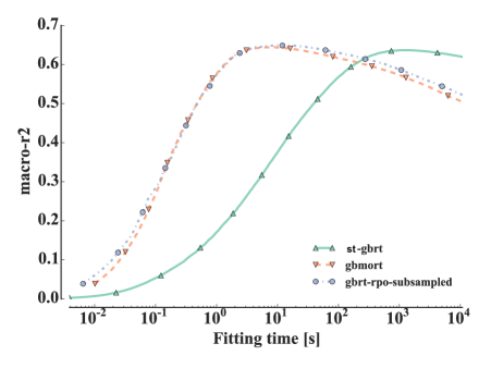
(a) Friedman1-chain

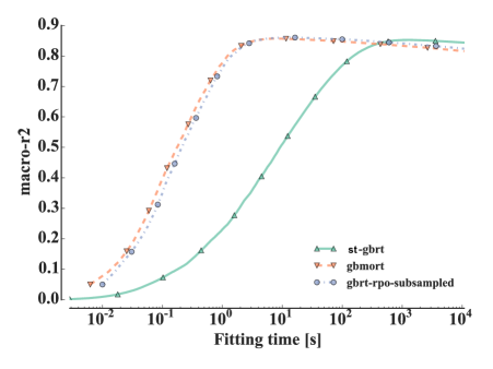
(b) Friedman1-group

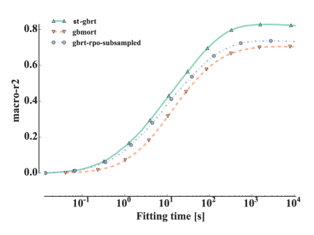
(c) Friedman1-ind

Figure 6.1: The convergence speed and the optimum reached are affected by the output correlation structure. The gbmort and gbrt-rpo-subsampled algorithms both exploit output correlations, which yields faster convergence and slightly better performance than st-gbrt on friedman1-chain and friedman1-group. However, st-gbrt converges to a better optimum than gbmort and gbrt-rpo-subsample when there is no output correlation as in friedman1-ind. (Model parameters: $k=p$, $n_{\max{}\_leaves}=2$, $\mu=0.1$)

On the friedman1-chain (see Figure 6.1a) and friedman1-group (see Figure 6.1b), gbmort and gbrt-rpo-subsampled converge more than 100 times faster (note the logarithmic scale of the abscissa) than single target. Furthermore, the optimal macro-$r^{2}$ is slightly better for gbmort and gbrt-rpo-subsampled than st-gbrt. Since all outputs are correlated on both datasets, gbmort and gbrt-rpo-susbsampled are exploiting the output structure to have faster convergence. The gbmort method exploits the output structure by filtering the output noise as the stump fitted at each iteration is the one that maximizes the reduction of the average output variance. By contrast, gbrt-rpo-subsample detects output correlations by optimizing the $\rho_{m}$ constant and then shares the information obtained by the current weak model with all other outputs.

On the friedman1-ind dataset (see Figure 6.1c), all three methods converge at the same rate. However, the single target strategy converges to a better optimum than gbmort and gbrt-rpo-subsample. Since all outputs are independent, single target enforces the proper correlation structure (see Figure 6.1c). The gbmort method has the worst performance as it assumes the wrong set of hypotheses. The gbrt-rpo-subsampled method pays the price of its flexibility by over-fitting the additive weight associated to each output, but less than gbmort.

This experiment confirms that enforcing the right correlation structure yields faster convergence and the best accuracy. Nevertheless, the output structure is unknown in practice. We need flexible approaches such as gbrt-rpo-subsampled that automatically detects and exploits the correlation structure.

23.2.3   Performance and output modeling assumption

The presence or absence of structures among the outputs have shown to affect the convergence speed of multi-output gradient boosting methods. As discussed in Cheng et al. (2010), we talk about conditionally independent outputs when:

$$P(y_{1},\ldots,y_{q}|x)=P(y_{1}|x)\cdots P(y_{q}|x)$$

and about unconditionally independent outputs when:

$$P(y_{1},\ldots,y_{q})=P(y_{1})\cdots P(y_{q}).$$

When the outputs are not conditionally independent and the loss function can not be decomposed over the outputs (eg., the subset $0-1$ loss), one might need to model the joint output distribution $P(y_{1},\ldots,y_{q}|x)$ to obtain a Bayes optimal prediction. If the outputs are conditionally independent however or if the loss function can be decomposed over the outputs, then a Bayes optimal prediction can be obtained by modeling separately the marginal conditional output distributions $P(y_{j}|x)$ for all $j$. This suggests that in this case, binary relevance / single target is not really penalized asymptotically with respect to multiple output methods for not considering the outputs jointly. In the case of an infinite sample size, it is thus expected to provide as good models as all the multiple output methods. Since in practice we have to deal with finite sample sizes, multiple output methods may provide better results by better controlling the bias/variance trade-off.

Let us study this question on the three synthetic datasets: friedman1-chain, friedman1-group or friedman1-ind. We optimize the hyper-parameters with a computational budget of 10000 weak models per hyper-parameter set. Five strategies are compared (i) the artificial-gbrt method, which assumes that the output structure is known and implements the optimal strategy on each problem as explained in Section 23.2.1, (ii) single target of gradient boosting regression trees (st-gbrt), (iii) gradient boosting with multi-output regression tree (gbmort, Algorithm 1) and gradient boosting with randomly sub-sampled outputs (iv) without relabelling (gbrt-rpo-subsampled, Algorithm 2) and (v) with relabelling (gbrt-relabel-rpo-subsampled, Algorithm 3). All boosting algorithms minimize the square loss, the absolute loss or their multi-outputs extension the $\ell_{2}$-norm loss.

We give the performance on the three tasks for each estimator in Table 6.1 and the p-value of Student’s paired $t$-test comparing the performance of two estimators on the same dataset in Table 6.2.

Table 6.1: All methods compared on the 3 artificial datasets. Exploiting the output correlation structure (if it exists) allows beating single target in a finite sample size, decomposable metric and conditionally independent output.

Dataset	friedman1-chain	friedman1-group	friedman1-ind
artificial-gbrt	$0.654\pm 0.015$(1)	$0.889\pm 0.009$(1)	$0.831\pm 0.004$(1)
st-gbrt	$0.626\pm 0.016$(5)	$0.873\pm 0.008$(5)	$0.830\pm 0.003$(2)
gbmort	$0.640\pm 0.008$(4)	$0.874\pm 0.012$(4)	$0.644\pm 0.010$(5)
gbrt-relabel-rpo-subsampled	$0.648\pm 0.015$(2)	$0.880\pm 0.009$(2)	$0.706\pm 0.009$(4)
gbrt-rpo-subsampled	$0.645\pm 0.013$(3)	$0.876\pm 0.007$(3)	$0.789\pm 0.003$(3)

Table 6.2: P-values given by Student’s paired $t$-test on the synthetic datasets. We highlight p-values inferior to $\alpha=0.05$ in bold. Note that the sign $<$ (resp. $>$) indicates that the estimator in the row has better (resp.lower) score than the column estimator.

	artificial-gbrt	st-gbrt	gbmort	gbrt-relabel-rpo-subsampled	gbrt-rpo-subsampled
Dataset friedman1-chain
artificial-gbrt		0.003(>)	0.16	0.34	0.24
st-gbrt	0.003(<)		0.11	0.04(<)	0.03(<)
gbmort	0.16	0.11		0.38	0.46
gbrt-relabel-rpo-subsampled	0.34	0.04(>)	0.38		0.57
gbrt-rpo-subsampled	0.24	0.03(>)	0.46	0.57
Dataset friedman1-group
artificial-gbrt		0.005(>)	0.009(>)	0.047(>)	0.006(>)
st-gbrt	0.005(<)		0.56	0.046(<)	0.17
gbmort	0.009(<)	0.56		0.15	0.63
gbrt-relabel-rpo-subsampled	0.047(<)	0.046(>)	0.15		0.04(>)
gbrt-rpo-subsampled	0.006(<)	0.17	0.63	0.04(<)
Dataset friedman1-ind
artificial-gbrt		0.17	2e-06(>)	2e-06(>)	1e-05(>)
st-gbrt	0.17		2e-06(>)	4e-06(>)	4e-06(>)
gbmort	2e-06(<)	2e-06(<)		9e-05(<)	6e-06(<)
gbrt-relabel-rpo-subsampled	2e-06(<)	4e-06(<)	9e-05(>)		3e-05(<)
gbrt-rpo-subsampled	1e-05(<)	4e-06(<)	6e-06(>)	3e-05(>)

As expected, we obtain the best performance if the output correlation structure is known with the custom strategies implemented with artifical-gbrt. Excluding this artificial method, the best boosting methods on the two problems with output correlations, friedman1-chain and friedman1-group, are the two gradient boosting approaches with output subsampling (gbrt-relabel-rpo-subsampled and gbrt-rpo-subsampled).

In friedman1-chain, the output correlation structure forms a chain as each new output is the previous one in the chain with a noisy output. Predicting outputs at the end of the chain, without using the previous ones, is a difficult task. The single target approach is thus expected to be sub-optimal. And indeed, on this problem, artificial-gbrt, gbrt-relabel-rpo-subsampled and gbrt-rpo-subsampled are significantly better than st-gbrt (with $\alpha=0.05$). All the multi-output methods, including gbmort, are indistinguishable from a statistical point of view, but we note that gbmort is however not significantly better than st-gbrt.

In friedman1-group, among the ten pairs of algorithms, four are not significantly different, showing a p-value greater than 0.05 (see Table 6.2). We first note that gbmort is not better than st-gbrt while exploiting the correlation. Secondly, the boosting methods with random output sub-sampling are the best methods. They are however not significantly better than gbmort and significantly worse than artificial-gbrt, which assumes the output structure is known. Note that gbrt-relabel-rpo-subsampled is significantly better than gbrt-rpo-subsampled.

In friedman1-ind, where there is no correlation between the outputs, the best strategy is single target which makes independent models for each output. From a conceptual and statistical point of view, there is no difference between artificial-gbrt and st-gbrt. The gbmort algorithm, which is optimal when all outputs are correlated, is here significantly worse than all other methods. The two boosting methods with output subsampling (gbrt-rpo-subsampled and gbrt-relabel-rpo-subsampled method), which can adapt themselves to the absence of correlation between the outputs, perform better than gbmort, but they are significantly worse than st-gbrt. For these two algorithms, we note that not relabelling the leaves (gbrt-rpo-subsampled) leads to superior performance than relabelling them (gbrt-relabel-rpo-subsampled). Since in friedman1-ind the outputs have disjoint feature support, the test nodes of a decision tree fitted on one output will partition the samples using these features. Thus, it is not suprising that relabeling the trees leaves actually deteriorates performance.

In the previous experiment, all the outputs were dependent of the inputs. However in multi-output tasks with very high number of outputs, it is likely that some of them have few or no links with the inputs, i.e., are pure noise. Let us repeat the previous experiments with the main difference that we add to the original 16 outputs 16 purely noisy outputs obtained through random permutations of the original outputs. We show the results of optimizing each algorithm in Table 6.3 and the associated p-values in Table 6.4. We report the macro-$r^{2}$ score computed either on all outputs (macro-$r^{2}$) including the noisy outputs or only on the 16 original outputs (half-macro-$r^{2}$). P-value were computed between each pair of algorithms using Student’s $t$-test on the macro $r^{2}$ score computed on all outputs.

We observe that the gbrt-rpo-subsampled algorithm has the best performance on friedman1-chain and friedman1-group and is the second best on the friedman1-ind, below st-gbrt. Interestingly on friedman1-chain and friedman1-group, this algorithm is significantly better than all the others, including gbmort. Since this latter method tries to fit all outputs simultaneously, it is the most disadvantaged by the introduction of the noisy outputs.

Table 6.3: Friedman datasets with noisy outputs.

friedman1-chain	half-macro-$r^{2}$	macro-$r^{2}$
st-gbrt	0.611 (4)	$0.265\pm 0.006$ (4)
gbmort	0.617 (3)	$0.291\pm 0.012$ (3)
gbrt-relabel-rpo-subsampled	0.628 (2)	$0.292\pm 0.006$ (2)
gbrt-rpo-subsampled	0.629 (1)	$0.303\pm 0.007$ (1)
Friedman1-group	half-macro-$r^{2}$	macro-$r^{2}$
st-gbrt	0.840 (3)	$0.364\pm 0.007$ (4)
gbmort	0.833 (4)	$0.394\pm 0.004$ (3)
gbrt-relabel-rpo-subsampled	0.855 (2)	$0.395\pm 0.005$ (2)
gbrt-rpo-subsampled	0.862 (1)	$0.414\pm 0.006$ (1)
Friedman1-ind	half-macro-$r^{2}$	macro-$r^{2}$
st-gbrt	0.806 (1)	$0.3536\pm 0.0015$ (1)
gbmort	0.486 (4)	$0.1850\pm 0.0081$ (4)
gbrt-relabel-rpo-subsampled	0.570 (3)	$0.2049\pm 0.0033$ (3)
gbrt-rpo-subsampled	0.739 (2)	$0.3033\pm 0.0021$ (2)

Table 6.4: P-values given by Student’s paired $t$-test on the synthetic datasets. We highlight p-values inferior to $\alpha=0.05$ in bold. Note that the sign $<$ (resp. $>$) indicates that the estimator in the row has better (resp.lower) score than the column estimator.

	st-gbrt	gbmort	gbrt-relabel-rpo-subsampled	gbrt-rpo-subsampled
Dataset friedman1-chain
st-gbrt		0.0009(<)	0.0002(<)	0.0002(<)
gbmort	0.0009(>)		0.86	0.04(<)
gbrt-relabel-rpo-subsampled	0.0002(>)	0.86		0.03(<)
gbrt-rpo-subsampled	0.0002(>)	0.04(>)	0.03(>)
Dataset friedman1-group
st-gbrt		0.0002(<)	0.0006(<)	0.0003(<)
gbmort	0.0002(>)		0.74	0.008(<)
gbrt-relabel-rpo-subsampled	0.0006(>)	0.74		0.002(<)
gbrt-rpo-subsampled	0.0003(>)	0.008(>)	0.002(>)
Dataset friedman1-ind
st-gbrt		1e-06(>)	1e-07(>)	1e-06(>)
gbmort	1e-06(<)		0.02(<)	6e-06(<)
gbrt-relabel-rpo-subsampled	1e-07(<)	0.02(>)		2e-06(<)
gbrt-rpo-subsampled	1e-06(<)	6e-06(>)	2e-06(>)

23.3   Effect of random projection

With the gradient boosting and random projection of the output space approaches (Algorithms 2 and 3), we have considered until now only sub-sampling a single output at each iteration as random projection scheme. In Section 23.3.1, we show empirically the effect of other random projection schemes such as Gaussian random projection. In Section 23.3.2, we study the effect of increasing the number of projections in the gradient boosting algorithm with random projection of the output space and relabelling (parameter $q$ of Algorithm  3). We also show empirically the link between Algorithm  3 and gradient boosting with multi-output regression tree (Algorithm 1).

23.3.1   Choice of the random projection scheme

Beside random output sub-sampling, we can combine the multi-output gradient boosting strategies (Algorithms 2 and 3) with other random projection schemes. A key difference between random output sub-sampling and random projections such as Gaussian and (sparse) Rademacher projections is that the latter combines together several outputs.

We show in Figures 6.2, 6.3 and 6.4 the LRAP or macro-$r^{2}$ score convergence of gradient boosting with randomly projected outputs (gbrt-rpo, Algorithm 2) respectively on the mediamill, delicious, and Friedman1-ind datasets with different random projection schemes.

The impact of the random projection scheme on convergence speed of gbrt-rpo (Algorithm 2) is very problem dependent. On the mediamill dataset, Gaussian, Achlioptas, or sparse random projections all improve convergence speed by a factor of 10 (see Figure 6.2) compared to subsampling randomly only one output. On the delicious (Figure 6.3) and friedman1-ind (Figure 6.4), this is the opposite: subsampling leads to faster convergence than all other projections schemes. Note that we have the same behavior if one relabels the tree structure grown at each iteration as in Algorithm 3 (results not shown).

Dense random projections, such as Gaussian random projections, force the weak model to consider several outputs jointly and it should thus only improve when outputs are somewhat correlated (which seems to be the case on mediamill). When all of the outputs are independent or the correlation is less strong, as in friedman1-ind or delicious, this has a detrimental effect. In this situation, sub-sampling only one output at each iteration leads to the best performance.

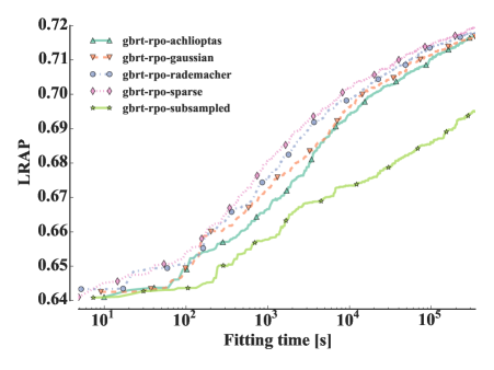
Figure 6.2: On the mediamill dataset, Gaussian, Achlioptas and sparse random projections with gbrt-rpo (Algorithm 2) show 10 times faster convergence in terms of LRAP score, than sub-sampling one output variable at each iteration. ($k=p$, stumps, $\mu=0.1$, logistic loss)

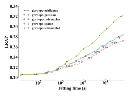
Figure 6.3: On the delicious dataset, Gaussian, Achlioptas and sparse random projections with gbrt-rpo (Algorithm 2) show 10 times faster convergence in terms of LRAP score, than sub-sampling one output variable at each iteration. ($k=p$, stumps, $\mu=0.1$, logistic loss)

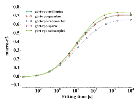
Figure 6.4: On the friedman1-ind dataset where there is no output correlation, gbrt-rpo (Algorithm 2) with one random subsampled output leads to a higher macro-$r^{2}$ score than using Gaussian, Achlioptas or sparse random projections. ($k=p$, stumps, $\mu=0.1$, square loss)

23.3.2   Effect of the size of the projected space

The multi-output gradient boosting strategy combining random projections and tree relabelling (Algorithm 3) can use more than one random projection ($q\geq 1$) by using multi-output trees as base learners. In this section, we study the effect of the size of the projected space $q$ in Algorithm 3. This approach corresponds to the one developed in Chapter 5 for random forest.

Figure 6.5 shows the LRAP score as a function of the fitting time for gbmort (Algorithm 1) and gbrt-relabel-rpo (Algorithm 3) with either Gaussian random projection (see Figure 6.5a) or output subsampling (see Figure 6.5b) for a number of projections $q\in\left\{1,98,196,491\right\}$ on the delicious dataset. In Figure 6.5a and Figure 6.5b, one Gaussian random projection or one sub-sampled output has faster convergence than their counterparts with a higher number of projections $q$ and gbmort at fixed computational budget. Note that when the number of projections $q$ increases, gradient boosting with random projection of the output space and relabeling becomes similar to gbmort.

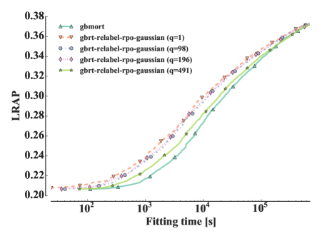
(a)

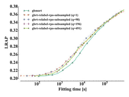
(b)

Figure 6.5: On the delicious dataset, LRAP score as a function of the boosting ensemble fitting time for gbrt-rpo-gaussian-relabel and gbrt-rpo-subsampled-relabel with different number of projections $q$. ($k=p$, stumps, $\mu=0.1$, logistic loss)

Instead of fixing the computational budget as a function of the training time, we now set the computational budget to 100 boosting steps. On the delicious dataset, gbrt-relabel-rpo (Algorithm 3) with Gaussian random projection yields approximately the same performance as gbmort with $q\geq 20$ random projections as shown in Figure 6.6a and reduces computing times by a factor 7 at $q=20$ projections (see Figure 6.6b).

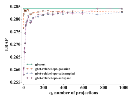
(a)

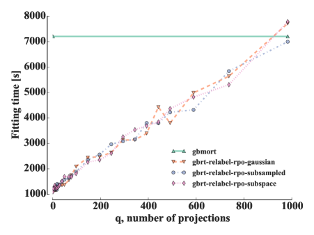
(b)

Figure 6.6: On delicious, increasing the number of random projections $q$ allows to reach the same LRAP score as gbmort at a significantly reduced computational cost. ($k=p$, stumps, $\mu=0.1$, $M=100$, logistic loss)

These experiments show that gradient boosting with random projection and relabelling (gbrt-relabel-rpo, Algorithm 3) is indeed an approximation of gradient boosting with multi-output trees (gbmort, Algorithm 1). The number of random projections $q$ influences simultaneously the bias-variance tradeoff and the convergence speed of Algorithm 3.

23.4   Systematic analysis over real world datasets

We perform a systematic analysis over real world multi-label classification and multi-output regression datasets. For this study, we evaluate the proposed algorithms: gradient boosting of multi-output regression trees (gbmort, Algorithm 1), gradient boosting with random projection of the output space (gbrt-rpo, Algorithm 2), and gradient boosting with random projection of the output space and relabelling (gbrt-relabel-rpo, Algorithm 3). For the two latter algorithms, we consider two random projection schemes: (i) Gaussian random projection, a dense random projection, and (ii) random output sub-sampling, a sparse random projection. They will be compared to three common and well established tree-based multi-output algorithms: (i) binary relevance / single target of gradient boosting regression tree (br-gbrt / st-gbrt), (ii) multi-output random forest (mo-rf) and (iii) binary relevance / single target of random forest models (br-rf / st-rf).

We will compare all methods on multi-label tasks in Section 23.4.1 and on multi-output regression tasks in Section 23.4.2. Following the recommendations of (Demšar, 2006), we use the Friedman test and its associated Nemenyi post-hoc test. Pairwise comparisons are also carried out using the Wilcoxon signed ranked test.

23.4.1   Multi-label datasets

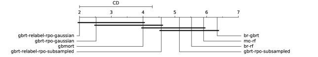
Figure 6.7: Critical difference diagram between algorithms on the multi-label datasets.

Table 6.5 and Table 6.6 show the performance of the random forest models and the boosting algorithms over the 21 multi-label datasets. The critical distance diagram of Figure 6.7 gives the ranks of the algorithms and has an associated Friedman test p-value of $1.36\times 10^{-10}$ with a critical distance of $2.29$ given by the Nemenyi post-hoc test ($\alpha=0.05$). Thus, we can reject the null hypothesis that all methods are equivalent. Table 6.7 gives the outcome of the pairwise Wilcoxon signed ranked tests.

The best average performer is gbrt-relabel-rpo-gaussian which is significantly better according to the Nemenyi post-hoc test than all methods except gbrt-rpo-gaussian and gbmort.

Gradient boosting with the Gaussian random projection has a significantly better average rank than the random output sub-sampling projection. Relabelling tree leaves allows to have better performance on the 21 multi-label dataset. Indeed, both gbrt-relabel-rpo-gaussian and gbrt-relabel-rpo-subsampled are better ranked and significantly better than their counterparts without relabelling (gbrt-rpo-gaussian and gbrt-rpo-subsampled). These results somewhat contrast with the results obtained on the artificial datasets, where relabelling was always counterproductive.

Among all compared methods, br-gbrt has the worst rank and it is significantly less good than all gbrt variants according to the Wilcoxon signed rank test. This might be actually a consequence of the constant budget in time that was allocated to all methods (see Section 23.1). All methods were given the same budget in time but, given the very slow convergence rate of br-gbrt, this budget may not allow to grow enough trees per output with this method to reach competitive performance.

We notice also that both random forests based methods (mo-rf and br-rf) are less good than all gbrt variants, most of the time significantly, except for br-gbrt. It has to be noted however that no hyper-parameter was tuned for the random forests. Such tuning could slightly change our conclusions, although random forests often work well with default setting.

Table 6.5: LRAP scores over 21 multi-label datasets (part 1).

	CAL500	bibtex	birds
br-gbrt	$0.505\pm 0.002$ (3.5)	$0.587\pm 0.007$ (6)	$0.787\pm 0.009$ (6)
br-rf	$0.484\pm 0.002$ (8)	$0.542\pm 0.005$ (8)	$0.802\pm 0.013$ (1)
gbmort	$0.501\pm 0.005$ (6)	$0.595\pm 0.005$ (4.5)	$0.772\pm 0.007$ (8)
gbrt-relabel-rpo-gaussian	$0.507\pm 0.009$ (1)	$0.607\pm 0.005$ (1)	$0.800\pm 0.017$ (2)
gbrt-relabel-rpo-subsampled	$0.499\pm 0.008$ (7)	$0.596\pm 0.005$ (3)	$0.790\pm 0.016$ (4)
gbrt-rpo-gaussian	$0.505\pm 0.006$ (3.5)	$0.600\pm 0.003$ (2)	$0.793\pm 0.017$ (3)
gbrt-rpo-subsampled	$0.506\pm 0.006$ (2)	$0.595\pm 0.007$ (4.5)	$0.779\pm 0.018$ (7)
mo-rf	$0.502\pm 0.003$ (5)	$0.553\pm 0.005$ (7)	$0.789\pm 0.012$ (5)
	bookmarks	corel5k	delicious
br-gbrt	$0.4463\pm 0.0038$ (7)	$0.291\pm 0.006$ (7)	$0.347\pm 0.002$ (8)
br-rf	$0.4472\pm 0.0019$ (6)	$0.273\pm 0.012$ (8)	$0.373\pm 0.004$ (6.5)
gbmort	$0.4855\pm 0.0016$ (2)	$0.312\pm 0.009$ (3.5)	$0.384\pm 0.003$ (3.5)
gbrt-relabel-rpo-gaussian	$0.4893\pm 0.0003$ (1)	$0.315\pm 0.007$ (1.5)	$0.389\pm 0.003$ (1)
gbrt-relabel-rpo-subsampled	$0.4718\pm 0.0034$ (4)	$0.310\pm 0.007$ (5)	$0.384\pm 0.003$ (3.5)
gbrt-rpo-gaussian	$0.4753\pm 0.0022$ (3)	$0.315\pm 0.010$ (1.5)	$0.386\pm 0.004$ (2)
gbrt-rpo-subsampled	$0.4621\pm 0.0026$ (5)	$0.312\pm 0.006$ (3.5)	$0.377\pm 0.003$ (5)
mo-rf	$0.4312\pm 0.0023$ (8)	$0.294\pm 0.010$ (6)	$0.373\pm 0.004$ (6.5)
	diatoms	drug-interaction	emotions
br-gbrt	$0.623\pm 0.007$ (7.5)	$0.271\pm 0.018$ (8)	$0.800\pm 0.022$ (7)
br-rf	$0.623\pm 0.011$ (7.5)	$0.310\pm 0.009$ (5)	$0.816\pm 0.009$ (1)
gbmort	$0.656\pm 0.012$ (4)	$0.304\pm 0.005$ (7)	$0.794\pm 0.014$ (8)
gbrt-relabel-rpo-gaussian	$0.725\pm 0.010$ (1)	$0.326\pm 0.008$ (1)	$0.802\pm 0.017$ (5.5)
gbrt-relabel-rpo-subsampled	$0.685\pm 0.012$ (3)	$0.322\pm 0.009$ (3)	$0.808\pm 0.021$ (3)
gbrt-rpo-gaussian	$0.702\pm 0.014$ (2)	$0.323\pm 0.011$ (2)	$0.804\pm 0.009$ (4)
gbrt-rpo-subsampled	$0.653\pm 0.013$ (5.5)	$0.312\pm 0.013$ (4)	$0.802\pm 0.007$ (5.5)
mo-rf	$0.653\pm 0.010$ (5.5)	$0.308\pm 0.007$ (6)	$0.810\pm 0.010$ (2)
	enron	genbase	mediamill
br-gbrt	$0.685\pm 0.006$ (6)	$0.989\pm 0.009$ (8)	$0.7449\pm 0.0020$ (8)
br-rf	$0.683\pm 0.005$ (7)	$0.994\pm 0.005$ (2)	$0.7819\pm 0.0009$ (1)
gbmort	$0.705\pm 0.004$ (2.5)	$0.990\pm 0.004$ (6)	$0.7504\pm 0.0013$ (7)
gbrt-relabel-rpo-gaussian	$0.705\pm 0.003$ (2.5)	$0.993\pm 0.006$ (3)	$0.7660\pm 0.0021$ (3)
gbrt-relabel-rpo-subsampled	$0.697\pm 0.004$ (5)	$0.990\pm 0.010$ (6)	$0.7588\pm 0.0013$ (5)
gbrt-rpo-gaussian	$0.706\pm 0.004$ (1)	$0.992\pm 0.007$ (4)	$0.7608\pm 0.0008$ (4)
gbrt-rpo-subsampled	$0.699\pm 0.005$ (4)	$0.990\pm 0.005$ (6)	$0.7519\pm 0.0006$ (6)
mo-rf	$0.676\pm 0.004$ (8)	$0.995\pm 0.004$ (1)	$0.7793\pm 0.0015$ (2)

Table 6.6: LRAP scores over 21 multi-label datasets (part 2).

	medical	protein-interaction	reuters
br-gbrt	$0.864\pm 0.006$ (3)	$0.294\pm 0.007$ (6)	$0.939\pm 0.0033$ (7)
br-rf	$0.821\pm 0.007$ (8)	$0.293\pm 0.006$ (7)	$0.9406\pm 0.0016$ (6)
gbmort	$0.867\pm 0.011$ (1.5)	$0.310\pm 0.007$ (2.5)	$0.9483\pm 0.0014$ (3)
gbrt-relabel-rpo-gaussian	$0.867\pm 0.019$ (1.5)	$0.310\pm 0.009$ (2.5)	$0.9508\pm 0.0009$ (1)
gbrt-relabel-rpo-subsampled	$0.856\pm 0.012$ (5)	$0.303\pm 0.003$ (4.5)	$0.9441\pm 0.0016$ (4)
gbrt-rpo-gaussian	$0.859\pm 0.017$ (4)	$0.311\pm 0.007$ (1)	$0.9486\pm 0.0021$ (2)
gbrt-rpo-subsampled	$0.851\pm 0.009$ (6)	$0.303\pm 0.003$ (4.5)	$0.9430\pm 0.0031$ (5)
mo-rf	$0.827\pm 0.006$ (7)	$0.288\pm 0.009$ (8)	$0.9337\pm 0.0021$ (8)
	scene	scop-go	sequence-funcat
br-gbrt	$0.880\pm 0.003$ (4)	$0.716\pm 0.047$ (8)	$0.678\pm 0.008$ (6)
br-rf	$0.876\pm 0.003$ (6)	$0.798\pm 0.004$ (2)	$0.658\pm 0.008$ (7)
gbmort	$0.886\pm 0.004$ (1)	$0.796\pm 0.007$ (3)	$0.699\pm 0.005$ (3)
gbrt-relabel-rpo-gaussian	$0.884\pm 0.006$ (2.5)	$0.788\pm 0.006$ (4)	$0.703\pm 0.007$ (2)
gbrt-relabel-rpo-subsampled	$0.879\pm 0.008$ (5)	$0.770\pm 0.010$ (6)	$0.685\pm 0.008$ (5)
gbrt-rpo-gaussian	$0.884\pm 0.005$ (2.5)	$0.775\pm 0.018$ (5)	$0.706\pm 0.007$ (1)
gbrt-rpo-subsampled	$0.875\pm 0.006$ (7)	$0.723\pm 0.016$ (7)	$0.691\pm 0.006$ (4)
mo-rf	$0.865\pm 0.003$ (8)	$0.800\pm 0.006$ (1)	$0.643\pm 0.003$ (8)
	wipo	yeast	yeast-go
br-gbrt	$0.706\pm 0.009$ (6)	$0.756\pm 0.009$ (8)	$0.499\pm 0.009$ (4.5)
br-rf	$0.633\pm 0.013$ (7)	$0.760\pm 0.008$ (3.5)	$0.463\pm 0.010$ (7)
gbmort	$0.762\pm 0.011$ (3)	$0.760\pm 0.007$ (3.5)	$0.504\pm 0.015$ (3)
gbrt-relabel-rpo-gaussian	$0.776\pm 0.012$ (1)	$0.762\pm 0.007$ (2)	$0.524\pm 0.012$ (1)
gbrt-relabel-rpo-subsampled	$0.751\pm 0.017$ (4)	$0.758\pm 0.005$ (5.5)	$0.496\pm 0.013$ (6)
gbrt-rpo-gaussian	$0.763\pm 0.010$ (2)	$0.763\pm 0.005$ (1)	$0.522\pm 0.012$ (2)
gbrt-rpo-subsampled	$0.724\pm 0.011$ (5)	$0.758\pm 0.008$ (5.5)	$0.499\pm 0.011$ (4.5)
mo-rf	$0.624\pm 0.018$ (8)	$0.757\pm 0.008$ (7)	$0.415\pm 0.014$ (8)

Table 6.7: P-values given by the Wilcoxon signed rank test on the multi-label datasets. We bold p-values below $\alpha=0.05$. Note that the sign $>$ (resp. $<$) indicates that the row estimator has superior (resp. inferior) LRAP score than the column estimator.

	br-gbrt	br-rf	gbmort	gbrt-relabel-rpo-gaussian	gbrt-relabel-rpo-subsampled	gbrt-rpo-gaussian	gbrt-rpo-subsampled	mo-rf
br-gbrt		0.79	0.001(<)	6e-05(<)	0.001(<)	0.0001(<)	0.003(<)	0.54
br-rf	0.79		0.01(<)	0.002(<)	0.02(<)	0.005(<)	0.07	0.29
gbmort	0.001(>)	0.01(>)		0.001(<)	0.36	0.04(<)	0.03(>)	0.02(>)
gbrt-relabel-rpo-gaussian	6e-05(>)	0.002(>)	0.001(>)		0.0002(>)	0.005(>)	7e-05(>)	0.0007(>)
gbrt-relabel-rpo-subsampled	0.001(>)	0.02(>)	0.36	0.0002(<)		0.0002(<)	0.02(>)	0.008(>)
gbrt-rpo-gaussian	0.0001(>)	0.005(>)	0.04(>)	0.005(<)	0.0002(>)		7e-05(>)	0.002(>)
gbrt-rpo-subsampled	0.003(>)	0.07	0.03(<)	7e-05(<)	0.02(<)	7e-05(<)		0.04(>)
mo-rf	0.54	0.29	0.02(<)	0.0007(<)	0.008(<)	0.002(<)	0.04(<)

23.4.2   Multi-output regression datasets

Table 6.8 shows the performance of the random forest models and the boosting algorithms over the 8 multi-output regression datasets. The critical distance diagram of Figure 6.8 gives the rank of each estimator. The associated Friedman test has a p-value of $0.3$. Given the outcome of the test, we can therefore not reject the null hypothesis that the estimator performances can not be distinguished. Table 6.9 gives the outcomes of the pairwise Wilcoxon signed ranked tests. They confirm the fact that all methods are very close to each other as only two comparisons show a p-value lower than 0.05 (st-rf is better than st-gbrt and gbrt-rpo-subsampled). This lack of statistical power is probably partly due here to the smaller number of datasets included in the comparison (8 problems versus 21 problems in classification).

If we ignore statistical tests, as with multi-label tasks, gbrt-relabel-rpo-gaussian has the best average rank and st-gbrt the worst average rank. This time however, gbrt-relabel-rpo-gaussian is followed by the random forest based algorithms (st-rf and mo-rf) and gbmort. Given the lack of statistical significance, this ranking should however be intrepreted cautiously.

Table 6.8: Performance over 8 multi-output regression dataset

	atp1d	atp7d	edm
gbmort	$0.80\pm 0.03$(5.5)	$0.63\pm 0.03$(2)	$0.39\pm 0.16$(3)
gbrt-relabel-rpo-gaussian	$0.81\pm 0.03$(3.5)	$0.66\pm 0.04$(1)	$0.25\pm 0.28$(8)
gbrt-relabel-rpo-subsampled	$0.79\pm 0.04$(7)	$0.54\pm 0.13$(7)	$0.35\pm 0.10$(5)
gbrt-rpo-gaussian	$0.80\pm 0.04$(5.5)	$0.54\pm 0.20$(7)	$0.36\pm 0.04$(4)
gbrt-rpo-subsampled	$0.81\pm 0.04$(3.5)	$0.54\pm 0.16$(7)	$0.31\pm 0.27$(7)
mo-rf	$0.82\pm 0.03$(2)	$0.6\pm 0.06$(4)	$0.51\pm 0.02$(1)
st-gbrt	$0.78\pm 0.05$(8)	$0.59\pm 0.08$(5)	$0.34\pm 0.14$(6)
st-rf	$0.83\pm 0.02$(1)	$0.61\pm 0.07$(3)	$0.47\pm 0.04$(2)
	oes10	oes97	scm1d
gbmort	$0.77\pm 0.05$(3.5)	$0.67\pm 0.07$(8)	$0.908\pm 0.003$(4.5)
gbrt-relabel-rpo-gaussian	$0.75\pm 0.04$(7.5)	$0.71\pm 0.07$(2.5)	$0.910\pm 0.004$(2.5)
gbrt-relabel-rpo-subsampled	$0.75\pm 0.06$(7.5)	$0.68\pm 0.07$(6)	$0.912\pm 0.003$(1)
gbrt-rpo-gaussian	$0.77\pm 0.03$(3.5)	$0.68\pm 0.08$(6)	$0.910\pm 0.004$(2.5)
gbrt-rpo-subsampled	$0.76\pm 0.02$(5.5)	$0.71\pm 0.08$(2.5)	$0.908\pm 0.004$(4.5)
mo-rf	$0.76\pm 0.04$(5.5)	$0.69\pm 0.05$(4)	$0.898\pm 0.004$(8)
st-gbrt	$0.79\pm 0.03$(1.5)	$0.68\pm 0.07$(6)	$0.905\pm 0.003$(7)
st-rf	$0.79\pm 0.03$(1.5)	$0.72\pm 0.05$(1)	$0.907\pm 0.004$(6)
	scm20d	water-quality
gbmort	$0.856\pm 0.006$(2)	$0.14\pm 0.01$(4.5)
gbrt-relabel-rpo-gaussian	$0.862\pm 0.006$(1)	$0.15\pm 0.01$(2)
gbrt-relabel-rpo-subsampled	$0.854\pm 0.007$(3)	$0.14\pm 0.02$(4.5)
gbrt-rpo-gaussian	$0.852\pm 0.006$(4)	$0.14\pm 0.01$(4.5)
gbrt-rpo-subsampled	$0.850\pm 0.007$(5)	$0.13\pm 0.02$(7.5)
mo-rf	$0.849\pm 0.007$(6.5)	$0.16\pm 0.01$(1)
st-gbrt	$0.836\pm 0.006$(8)	$0.13\pm 0.02$(7.5)
st-rf	$0.849\pm 0.006$(6.5)	$0.14\pm 0.01$(4.5)

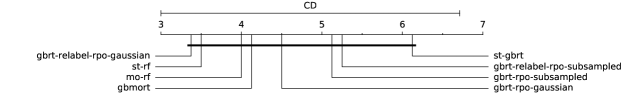
Figure 6.8: Critical difference diagram between algorithm on the multi-output regression datasets.

Table 6.9: P-value given by the Wilcoxon signed rank test on multi-output regression datasets. We bold p-values below $\alpha=0.05$. Note that the sign $>$ (resp. $<$) indicates that the row estimator has superior (resp. inferior) macro-$r^{2}$ score than the column estimator.

	st-gbrt	st-rf	gbmort	gbrt-relabel-rpo-gaussian	gbrt-relabel-rpo-subsampled	gbrt-rpo-gaussian	gbrt-rpo-subsampled	mo-rf
st-gbrt		0.02(<)	0.26	0.58	0.78	0.67	0.89	0.16
st-rf	0.02(>)		0.33	0.67	0.09	0.09	0.04(>)	0.58
gbmort	0.26	0.33		0.4	0.16	0.67	0.4	0.48
gbrt-relabel-rpo-gaussian	0.58	0.67	0.4		0.16	0.4	0.48	0.58
gbrt-relabel-rpo-subsampled	0.78	0.09	0.16	0.16		0.16	1	0.07
gbrt-rpo-gaussian	0.67	0.09	0.67	0.4	0.16		0.48	0.26
gbrt-rpo-subsampled	0.89	0.04(<)	0.4	0.48	1	0.48		0.4
mo-rf	0.16	0.58	0.48	0.58	0.07	0.26	0.4

24   Conclusions

In this chapter, we have first formally extended the gradient boosting algorithm to multi-output tasks leading to the “multi-output gradient boosting algorithm” (gbmort). It sequentially minimizes a multi-output loss using multi-output weak models considering that all outputs are correlated. By contrast, binary relevance / single target of gradient boosting models fit one gradient boosting model per output considering that all outputs are independent. However in practice, we do not expect to have either all outputs independent or all outputs dependent. So, we propose a more flexible approach which adapts automatically to the output correlation structure called “gradient boosting with random projection of the output space” (gbrt-rpo). At each boosting step, it fits a single weak model on a random projection of the output space and optimize a multiplicative weight separately for each output. We have also proposed a variant of this algorithm (gbrt-relabel-rpo) only valid with decision trees as weak models: it fits a decision tree on the randomly projected space and then it relabels tree leaves with predictions in the original (residual) output space. The combination of the gradient boosting algorithm and the random projection of the output space yields faster convergence by exploiting existing correlations between the outputs and by reducing the dimensionality of the output space. It also provides new bias-variance-convergence trade-off potentially allowing to improve performance.

We have evaluated in depth these new algorithms on several artificial and real datasets. Experiments on artificial problems highlighted that gb-rpo with output subsampling offers an interesting tradeoff between single target and multi-output gradient boosting. Because of its capacity to automatically adapt to the output space structure, it outperforms both methods in terms of convergence speed and accuracy when outputs are dependent and it is superior to gbmort (but not st-rt) when outputs are fully independent. On the 29 real datasets, gbrt-relabel-rpo with the denser Gaussian projections turns out to be the best overall approach on both multi-label classification and multi-output regression problems, although all methods are statistically undistinguisable on the regression tasks. Our experiments also show that gradient boosting based methods are competitive with random forests based methods. Given that multi-output random forests were shown to be competitive with several other multi-label approaches in Madjarov et al. (2012), we are confident that our solutions will be globally competitive as well, although a broader empirical comparison should be conducted as future work. One drawback of gradient boosting with respect to random forests however is that its performance is more sensitive to its hyper-parameters that thus require careful tuning. Although not discussed in this chapter, besides predictive performance, gbrt-rpo (without relabeling) has also the advantage of reducing model size with respect to mo-rf (multi-output random forests) and gbmort, in particular in the presence of many outputs. Indeed, in mo-rf and gbmort, one needs to store a vector of the size of the number of outputs per leaf node. In gbrt-rpo, one needs to store only one real number (a prediction for the projection) per leaf node and a vector of the size of the number of outputs per tree ($\rho_{m}$). At fixed number of trees and fixed tree complexity, this could lead to a strong reduction of the model memory requirement when the number of labels is large. Note that the approach proposed in Chapter 5 does not solve this issue because of leaf node relabeling. This could be addressed by desactivating leaf relabeling and inverting the projection at prediction time to obtain a prediction in the original output space, as done for example in Hsu et al. (2009); Kapoor et al. (2012); Tsoumakas et al. (2014). However, this would be at the expense of computing times at prediction time and of accuracy because of the potential introduction of errors at the decoding stage. Finally, while we restricted our experiments here to tree-based weak learners, Algorithms 1 and 2 are generic and could exploit respectively any multiple output and any single output regression method. As future work, we believe that it would interesting to evaluate them with other weak learners.

Part III   Exploiting sparsity for growing and compressing decision trees

$\ell_{1}$-based compression of random forest models

Remark 24.15.

Outline Random forests are effective supervised learning methods applicable to large-scale datasets. However, the space complexity of tree ensembles, in terms of their total number of nodes, is often prohibitive, specially in the context of problems with large sample sizes and very high-dimensional input spaces. We propose to study their compressibility by applying a $\ell_{1}$-based regularization to the set of indicator functions defined by all their nodes. We show experimentally that preserving or even improving the model accuracy while significantly reducing its space complexity is indeed possible.

This chapter extends on previous work published in

Arnaud Joly, François Schnitzler, Pierre Geurts, and Louis Wehenkel. L1-based compression of random forest models. In European Symposium on Artificial Neural Networks, Computational Intelligence and Machine Learning, 2012.

High-dimensional supervised learning problems, e.g. in image exploitation and bioinformatics, are more frequent than ever. Tree-based ensemble methods, such as random forests Breiman (2001) and extremely randomized trees Geurts et al. (2006a), are effective variance reduction techniques offering in this context a good trade-off between accuracy, computational complexity, and interpretability. The number of nodes of a tree ensemble grows as $nM$ ($n$ being the size of the learning sample and $M$ the number of trees in the ensemble). Empirical observations show that the variance of individual trees increases with the dimension $p$ of the original feature space used to represent the inputs of the learning problem. Hence, the number $M(p)$ of ensemble terms yielding near-optimal accuracy, which is proportional to this variance, also increases with $p$. The net result is that the space complexity of these tree-based ensemble methods will grow as $nM(p)$, which may jeopardize their practicality in large scale problems, or when memory is limited.

While pruning of single tree models is a standard approach, less work has been devoted to pruning ensembles of trees. On the one hand, Geurts (2000) proposes to transpose the classical cost-complexity pruning of individual trees to ensembles. On the other hand, Meinshausen (2010); Friedman and Popescu (2008); Meinshausen et al. (2009) propose to improve model interpretability by selecting optimal rule subsets from tree-ensembles. Another approach to reduce complexity and/or improve accuracy of ensembles of trees is to merely select an optimal subset of trees from a very large ensemble generated in a random fashion at the first hand (see, e.g. Bernard et al. (2009); Martinez-Muoz et al. (2009)).

To further investigate the feasibility of reducing the space complexity of tree-based ensemble models, we consider in this chapter the following method Joly et al. (2012): (i) build an ensemble of trees; (ii) apply to this ensemble a ‘compression step’ by reformulating the tree-ensemble based model as a linear model in terms of node indicator functions and by using an $\ell_{1}$-norm regularization approach - à la Lasso Tibshirani (1996b) - to select a minimal subset of these indicator functions while maintaining predictive accuracy. We propose an algorithmic framework and an empirical investigation of this idea, based on three complementary datasets, and we show that indeed it is possible to so compress significantly tree-based ensemble models, both in regression and in classification problems. We also observe that the compression rate and the accuracy of the compressed models further increase with the ensemble size $M$, even beyond the number $M(p)$ of terms required to ensure convergence of the variance reduction effect.

The rest of this chapter is organized as follows: Section 25 introduces the $\ell_{1}q$-norm based compression algorithm of random forests; Section 26 provides our empirical study and Section 27 concludes and describes further perspectives.

25   Compressing tree ensembles by $\ell_{1}$-norm regularization

From an ensemble of $M$ decision trees, one can extract a set of node indicator functions as follows: each indicator function $1_{m,l}(x)$ is a binary variable equal to 1 if the input vector $x$ reaches the $l$th node in the $m$th tree, $0$ otherwise. Using these indicator functions, the output predicted by the model may be rewritten as Geurts et al. (2006a); Vens and Costa (2011):

$$\hat{f}(x)=\frac{1}{M}\sum_{m=1}^{M}\sum_{l=1}^{N_{m}}w_{m,l}\,1_{m,l}(x),$$ (7.1)

where $N_{m}$ is the number of nodes in the $m$th tree and $w_{m,l}$ is equal to the leaf-label if node $(m,l)$ is a leaf and to zero if it is an internal node.

We can therefore interpret a tree building algorithm as the (random) inference of a new representation which lifts the original input space $\mathcal{X}$ towards the space $\mathcal{Z}$ of dimension $q=\sum_{m=1}^{M}N_{m}$ by

$$z(x)=\left(1_{1,1}(x),\ldots,1_{1,N_{1}}(x),\ldots{},1_{M,1}(x),\ldots,1_{M,N_{M}}(x)\right).$$

As an illustration, Figure 7.1 shows a set of three decision trees with respective sizes 7, 7 and 5 nodes. The propagation of a sample $x_{s}$ through the forest makes it pass trough nodes 1.1, 1.2, 1.5 in the left tree, nodes 2.1, 2.2, 2.5 in the middle tree and nodes 3.1, 3.3 and 3.4 in the left tree (highlighted in orange).

Figure 7.1: From a random forest model, one can lift the original input space representation of a sample $x_{s}$ toward the node indicator space $\mathcal{Z}$.

We propose to compress the tree ensemble by applying a variable selection method to its induced feature space $\mathcal{Z}$. Namely, by $\ell_{1}$-regularization we can search for a linear model by solving the following optimization problem:

$$\left(\beta_{j}^{*}(t)\right)_{j=0}^{q}=\arg\min_{\beta}\sum_{i=1}^{n}\left(y^{i}-\beta_{0}-\sum_{j=1}^{q}\beta_{j}\,z_{j}(x^{i})\right)^{2}$$

s.t. $$\sum_{j=1}^{q}|\beta_{j}|\leq t.$$ (7.2)

This optimization problem, also called Lasso Tibshirani (1996b) (see Section 4.1), has received much attention in the past decade and is particularly successful in high dimension. The $\ell_{1}$-norm constraint leads to a sparse solution: only a few weights $\beta_{j}$ will be non zero, and their number tends to zero with $t\rightarrow 0$; the optimal value $t^{*}$ of $t$ is problem specific and is typically adjusted by cross-validation.

In order to solve Equation 7.2 for growing values of $t$, we use the ‘incremental forward stagewise regression’ algorithm Hastie et al. (2007) solving the monotone Lasso which imposes that each $\beta^{*}_{j}(t)$ increases monotonically with $t$. This version deals indeed better with many correlated variables, which is relevant in our setting, since each node indicator function is highly correlated with those of its neighbor nodes in the tree from which it originates. The final weights $\beta_{j}^{*}(t^{*})$ may be exploited to prune the randomized tree ensemble: a test node can be deleted if all its descendants correspond to $\beta_{j}^{*}(t^{*})=0$.

Starting from a forest model $\hat{f}$, a value of parameter $t$, and a sample $\mathcal{S}$, the tree ensemble compression procedure is described in Algorithm 1.

Algorithm 1 $\ell_{1}$-based compression of tree ensemble model $\hat{f}$ using a sample $\mathcal{S}=\{x^{i},y^{i}\in\mathcal{X}\times\mathcal{Y}\}_{i=1}^{n}$

1:function ForestCompression($\mathcal{S}$, $\hat{f}$, t)

2:     Lift the sample $\mathcal{S}$ to the random forest space $\mathcal{Z}$

$$\mathcal{S}_{z}=\{(z(x^{i}),y^{i})\in\mathcal{Z}\times\mathcal{Y}\}_{(x,y)\in\mathcal{S}}$$

with the induced feature space by the forest model $\hat{f}$

$$z(x)=\left(1_{1,1}(x),\ldots,1_{1,N_{1}}(x),\ldots{},1_{M,1}(x),\ldots,1_{M,N_{M}}(x)\right).$$

3:     Select weight vector $\beta^{*}(t)$ over $\mathcal{Z}$ through $\ell_{1}$ minimization

$$\left(\beta_{j}^{*}(t)\right)_{j=0}^{q}=\arg\min_{\beta}\sum_{i=1}^{n}\left(y^{i}-\beta_{0}-\sum_{j=1}^{q}\beta_{j}\,z_{j}(x^{i})\right)^{2}$$

s.t. $$\sum_{j=1}^{q}|\beta_{j}|\leq t.$$

4:     Compress the random forest model $\hat{f}$ using vector $\beta^{*}(t)$

5:     return The compressed model.

6:end function

Note that in practice both the forest construction and the generation of its sequence of compressed versions for growing values of $t$ may use the same sample (the learning set). A separate validation set is however required to select the optimal value of parameter $t$. This is similar to what is done with the pruning of a single decision tree (see Section 11).

26   Empirical analysis

In the following experiments, datasets are pre-whitened: input/output data are translated to zero mean and rescaled to unit variance. All results shown are averaged over $50$ runs in order to avoid randomization artifacts.

Each one of these runs consisted of first generating a training set, and a testing set, and then working as follows. When using the monotone Lasso, we apply the incremental forward stagewise algorithm with a step size $\epsilon=0.01$. The optimal number of steps $n_{step}^{*}$ or the optimal point $t^{*}=n_{step}^{*}\epsilon$ was chosen by ten-fold cross-validation $t_{cv}^{*}$ over the training set (to this end, we used a quadratic loss in regression and a $0-1$ loss in classification). More precisely, the training set is first divided ten times through cross-validation into a learning set, used both to fit a forest model and to run the incremental forward stagewise algorithm on it, and into a validation set, to estimate the losses of the resulting sequence of compressed forests. For each fold, we assess the model fitted over the training set using the validation set with increasing values of $t$ by steps of $\epsilon$. For each value of $t$, the ten model losses are averaged. The optimal value of $t^{*}$ and the corresponding model compression level are those leading to the best average loss over the ten folds. The model is then refitted using the entire training set with $t=t^{*}$.

Below, we will apply our approach while using the extremely randomized trees method Geurts et al. (2006a) to grow the forests (abbreviated by “ET”) and we denote their $\ell_{1}$-regularization-based compressed version “rET”.

We present an overall performance analysis in Section 26.1. Later on, we enhance our comprehension of the pruning algorithm by studying the effect of the regularization parameter $t$ in Section 26.2 and of the complexity of the initial forest model by varying the pre-pruning rule values $n_{\min}$, the minimum number of samples to split, and $M$, the number of trees, in Section 26.3. While in these last two sections, we focus our analysis on models obtained on the Friedman1 problem, we notice that similar conclusions can also be drawn for Two-norm and SEFTi datasets.

26.1   Overall performances

We have evaluated our approach on two regression datasets Friedman1 and SEFTi and one classification dataset Two-norm (see Appendix 10 for their description).

We have used a set of representative meta-parameter values ($K$, $n_{\min}$ and $M$) of the Extra-Trees algorithm (see Table 7.1). Accuracies are measured on the test sample and complexity is measured by the number of test nodes of the ET and rET models (the compression factor being the ratio of the former to the latter). We observe a compression factor between 9 and 34, a slightly lower error for the rET model than for the ET model on the two regression problems (Friedman1 and SEFTi) and the opposite on Two-norm. To compare, we show the results obtained with the linear Lasso based on the original features (its complexity is measured by the number of kept features): it is much less accurate than both ET and rET on the (non-linear) regression problems (Friedman1 and SEFTi), but superior on the (linear) classification problem (Two-norm).

Table 7.1: Overall assessment (parameters of the Extra-Tree method: $M=100$; $K=p$; $n_{\min}=1$ on Friedman1 and Two-norm, $n_{\min}=10$ on SEFTi).

Datasets	Error			Complexity
	ET	rET	Lasso	ET	rET	ET/rET	Lasso
Friedman1	$0.19587$	$0.18593$	$0.282441$	$29900$	$\leavevmode\nobreak\ 885$	$34$	$\leavevmode\nobreak\ 4$
Two-norm	$0.04177$	$0.06707$	$0.033500$	$\leavevmode\nobreak\ 4878$	$\leavevmode\nobreak\ 540$	$\leavevmode\nobreak\ 9$	$20$
SEFTi	$0.86159$	$0.84131$	$0.988031$	$39436$	$2055$	$19$	$14$

Side experiments (results not provided) show that changing the value of parameter $K$ does not influence significantly the final accuracy and complexity on the Two-norm and Friedman1 datasets, while for SEFTi, accuracy increases strongly with $K$ (presumably due to a large number of noisy and/or irrelevant features) with however little impact on the final complexity.

26.2   Effect of the regularization parameter $t$.

The complexity of the regularized ET model is shrunk with the $\ell_{1}$-norm constraint of Equation 7.2 in a way depending on the value of $t$. As shown in Figure 7.2(a), an increase of $t$ decreases the error of rET until $t=3$, leading to a complexity (Figure 7.2(b)) of about 900 test nodes. Notice that in general the rET model eventually overfits when $t$ becomes large, although this is not visible on the range of values displayed in Figure 7.2(a) as the algorithm stops before.

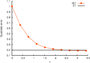
(a) Estimated risk

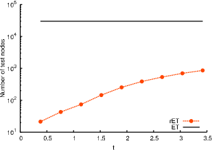
(b) Complexity

Figure 7.2: An increase of $t$ decreases the error of rET until t = 3 with drastic pruning (Friedman1, $M=100$, $K=p=10$ and $n_{\min}=1$).

26.3   Influence of the Extra-Tree meta parameters $n_{\min}$ and $M$.

The complexity of an ET model grows (linearly) with the size of the ensemble $M$ and is inversely proportional to its pre-pruning parameter $n_{\min}$.

Figure 7.3 shows the effect of $n_{\min}$ on both ET and rET. Interestingly, the accuracy and the complexity of the rET model are both more robust with respect to the choice of the precise value of $n_{\min}$ than those of the ET model, specially for the smaller values of $n_{\min}$ ($n_{\min}\leq 10$, in Figures 7.3).

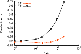
(a) Estimated risk

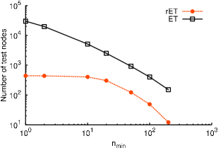
(b) Complexity

Figure 7.3: The accuracy and complexity of an rET model does not depend on $n_{\min}$, for $n_{\min}$ small enough (Friedman1, $M=100$, $K=p=10$ and $t=t_{cv}^{*}$).

Figure 7.4 shows the effect of $M$ on both ET and rET models. We observe that increasing the value of $M$ beyond the value $M(p)$ where variance reduction has stabilized ($M(p)\simeq 100$ in Figure 7.4) allows to further improve the accuracy of the rET model without increasing its complexity.

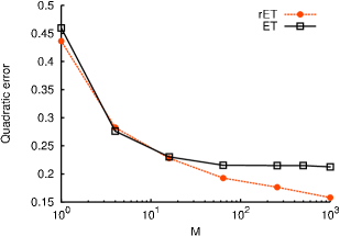
(a) Estimated risk

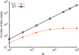
(b) Complexity

Figure 7.4: After variance reduction has stabilized ($M\simeq 100$), further increasing $M$ keeps enhancing the accuracy of the rET model without increasing complexity (Friedman1, $n_{\min}=10$, $K=p=10$ and $t=t_{cv}^{*}$).

27   Conclusion

Compression of randomized tree ensembles with $\ell_{1}$-norm regularization leads to a drastic reduction of space complexity while preserving accuracy. The complexity of the pruned model does not seem to be directly related to the complexity of the original forest, i.e. the number and complexity of each randomized tree, as long as this forest has explored a large enough space of variable interactions.

The strong compressibility of large randomized tree ensemble models suggests that it could be possible to design novel algorithms based on tree-based randomization which would scale in a better way to very high-dimensional input spaces than the existing methods. To achieve this, one open question is how to get the compressed tree ensemble directly, i.e. without generating a huge randomized tree ensemble and then pruning it.

Tree-based ensemble models may be interpreted as lifting the original input space towards a (randomly generated) high-dimensional discrete and sparse representation, where each induced feature corresponds to the indicator function of a particular tree node, and takes the value $1$ for a given observation if this observation reaches this node, and $0$ otherwise. The dimension of this representation is on the order of $nM(p)$, but the number $s$ of non-zero components for a given observation is only on the order of $M(p)\log n$. Compressed sensing theory Candès and Wakin (2008) tells us that high-dimensional sparsely representable observations may be compressed by projecting them on a random subspace of dimension proportional to $s\log p$, where $p$ is the original dimension of the observations and $s\ll p$ is the number of non-zero terms in their sparse representation basis. This suggests that one could reduce the space complexity of tree-based method by applying compressed sensing to their original input feature space if its dimension is high, and/or to their induced feature space if $nM(p)$ is too large.

Since the publication of our work on this subject, several authors have proposed similar ideas to post-prune a fully grown random forest model: Ren et al. (2015) propose to iteratively remove or re-weight the leaves of the random forest model, while Duroux and Scornet (2016) study the impact of pre-pruning on random forest models.

Exploiting input sparsity with decision tree

Remark 27.16.

Outline Many supervised learning tasks, such as text annotation, are characterized by high dimensional and sparse input spaces where the input vectors of each sample has only a few non zero values. We show how to exploit algorithmically the input space sparsity within decision tree methods. It leads to significant speed up both on synthetics and real datasets, while leading to exactly the same model. We also reduce the required memory to grow such models by exploiting sparse memory storage instead of dense memory storage for the input matrix.

This contribution is a joint work with Fares Hedayati and Panagiotis Papadimitriou, working at www.upwork.com. The outcome of this research has been proposed and merged in the scikit-learn Buitinck et al. (2013); Pedregosa et al. (2011) open source package.

Many machine learning tasks such as text annotation usually require training over very big datasets with millions of web documents. Such tasks require defining a mapping between the raw input space and the output space. For example in text classification, a text document (raw input space) is usually mapped to a vector whose dimensions correspond to all of the possible words in a dictionary and the values of the vector elements are determined by the frequency of the words in the document. Although such vectors have many dimensions, they are often sparsely representable. For instance, the number of unique words associated to a text document is actually small compared to the number of words of a given language. We describe those samples with sparse input vectors as having a few non zero values.

Exploiting the low density, i.e. the fraction of non zero elements, and the high sparsity, i.e. the fraction of zero elements, is key to address such high dimensional supervised learning tasks. Many models directly formulate their entire algorithm to exploit the input sparsity. Linear models such as logistic regression or support vector machine harness the sparsity by expressing most of their operations as a set of linear algebra operations such as dot products who directly exploit the sparsity to speed up computations.

Unfortunately, decision tree methods are not expressible only through linear algebra operations. Decision tree methods are recursively partitioning the input space by searching for the best possible splitting rules. As a consequence, most machine learning packages either do not support sparse input vectors for tree-based methods, only support stumps (decision tree with only one internal node) or have a sub-optimal implementation through the simulation of a random access memory as in the dense case. The only solution is often to densify the input space which leads first to severe memory constraints and then to slow training time.

In Section 28, we present efficient algorithms to grow vanilla decision trees, boosting and random forest methods on sparse input data. In Section 29, we describe how to adapt the prediction algorithm of these models to sparse input data. In Section 30, we show empirically the speed up obtained by fitting decision trees with this input sparsity aware implementation.

28   Tree growing

During the decision tree fitting, the tree growing algorithm (see Algorithm 2) interacts with the input space at two key points:

1. during the search of a splitting rule $s_{t}$ using a sample set $\mathcal{L}_{t}$ at the expansion of node $t$ (see line 10 of Algorithm 2);

2. during the data partitioning of the sample $\mathcal{L}_{t}$ into a left and a right partition following the splitting rule $s_{t}$ at node $t$ (see line 11 of Algorithm 2).

In this section, we show how to adapt decision tree at these three key points to handle sparsely expressed data. While at the same time, we will show how to harness the sparsity to speed up the original algorithm. We first explain how node splitting is implemented in standard decision trees in Section 28.1 and then explain our efficient implementation for sparse input data in Section 28.2. In Section 28.3, we further describe how to propagate samples with sparse input during the decision tree growing.

28.1   Standard node splitting algorithm

During the decision tree growth, the crux of the tree growing algorithm in high dimensional input space is the search of the best possible local splitting rule $s_{t}$ (as described in Section 10.1). Given a learning set $\mathcal{L}_{t}$ reaching a node $t$, we search for the splitting rule $s_{t}$ among all the possible binary and axis-wise splitting rules $\Omega(\mathcal{L}_{t})$. We strive to maximize the impurity reduction $\Delta I$ obtained by dividing the sample set $\mathcal{L}_{t}$ into two partitions $(\mathcal{L}_{t,r},\mathcal{L}_{t,l})$. The splitting rule selection problem (line 10 of the tree growing Algorithm 2) is written as

$$s_{t}=\arg\max_{s\in\Omega(\mathcal{L}_{t})}\Delta I(\mathcal{L}_{t},\mathcal{L}_{t,l},\mathcal{L}_{t,r})$$ (8.1)

with

$$\Omega(\mathcal{L}_{t})= \Bigg{\{}s:s\in\bigcup_{j\in\{1,\ldots,p\}}Q(x_{j}),$$

$$\quad\mathcal{L}_{t,l}=\{(x,y)\in\mathcal{L}_{t}:s(x)=1\},$$

$$\quad\mathcal{L}_{t,r}=\{(x,y)\in\mathcal{L}_{t}:s(x)=0\},$$

$$\quad\mathcal{L}_{t,l}\not=\emptyset,\mathcal{L}_{t,r}\not=\emptyset\Bigg{\}}$$ (8.2)

where $Q(x_{j})$ is the set of all splitting rules associated to an input variable $x_{j}$.

Decision tree libraries carefully optimize this part of the algorithm to have the proper computational complexity with a low constant. A careful design of the algorithm for instance does not move around samples according to the partitions, but instead move an identification number linked to each sample. The learning set $\mathcal{L}$ is implemented as an array of row indices $L$ linked to the rows of the input matrix $X$ and the output matrix $Y$. The sample set $\mathcal{L}_{t}$ reaching a node $t$ is implemented as a slice of the array $L[start_{t}:end_{t}[$ where the elements from the $start_{t}$ to the $`end_{t}-1`$ indices gives the indices of the samples reaching node $t$.

Let us take a small example with a set of $10$ training samples $L=[0,\,1\,,\cdots,9]$ illustrating the management of the array $L$. During the tree growth (see Algorithm 2) when we partition the sample set $\mathcal{L}_{t}=\{1,\ldots,10\}$ into two sample sets $\mathcal{L}_{t,l}=\{9,\,1,\,5,\,3\}$ and $\mathcal{L}_{t,r}=\{2,\,7,\,6,\,4,\,8,\,0\}$. In practice, we modify the array $L$ such that from 0 to $|\mathcal{L}_{1,l}|=4$ (resp. from $|\mathcal{L}_{1,l}|=4$ to $|\mathcal{L}_{1}|=10$) are located the samples of the left child (resp. right child). It leads to

$$L=[{\color[rgb]{1,.5,0}9,\,1,\,5,\,3},\,2,\,7,\,6,\,4,\,8,\,0].$$

We represent each sample set $\mathcal{L}_{t}$ as a slice $[start:end[$, a chunk, of the array $L$. The sample set $\mathcal{L}_{1,l}$ is the slice $[0:4[$ of $L$, while the sample set $\mathcal{L}_{1,r}$ is the slice $[4:10[$ of $L$. Now if the right node $\mathcal{L}_{1,r}$ is further split into a left node with samples $\{6,0\}$ and a right node with samples $\{2,7,4,8\}$ (in orange), then $L[4:10[$ is further modified to reflect the split:

$$L=[9,\,1,\,5,\,3,\,{\color[rgb]{1,.5,0}2,\,7,\,4,\,8},\,6,\,0].$$

To further speed up the best splitting rule search with ordered variables, we sort the possible thresholds associated to an ordered input variable $x_{j}$ (programmatically $sort(X_{j}[L[start_{t}:end_{t}[[)$). By sorting the possible thresholds sets, we can evaluate the impurity measure $I$ and the impurity reduction $\Delta I$ in an online fashion. For instance, the Gini index and entropy criteria can be computed by updating the class frequency in the left and right split when moving from one splitting threshold to the next.

28.2   Splitting rules search on sparse data

To handle sparse input data with decision trees, we need efficient procedures to select the best splitting rules $s_{t}$ among all the possible splitting rules knowing that we have a high proportion of zeros in the input matrix $X$. In this section, we propose an efficient method to exploit the sparsity of the input space with decision tree models. Our method takes advantage of the input sparsity by avoiding sorting sample sets of a node along a feature unless there are non zero elements at this feature. This approach speeds up training substantially as extracting the possible threshold values and sorting them is a costly but essential and ubiquitous component of tree-based models.

The splitting rule search algorithm for an ordered variable $x_{j}$ at a node $t$ is divided in two parts (see Algorithm 1): (i) to extract efficiently the non zero values associated to $x_{j}$ in the sample partition $\mathcal{L}_{t}$ (line 3) and (ii) to search separately among the splitting rules with the positive, negative or zero threshold (line 4).

Algorithm 1 Search for the best splitting rule $s_{t}^{*}$ given a sparse input matrix $X$ and a set of samples $\mathcal{L}_{t}$

1:function FindBestSparseSplit($X$, $\mathcal{L}_{t}$)

2:     for $j=1$ to $p$ do

3:          Extract strictly positive $X_{j,pos}$ and strictly negatives $X_{j,neg}$ values from $X_{j}$ given $\mathcal{L}_{t}$.

4:          Search for the best splitting rule of the form $s_{j}^{*}(x)=x_{j}\leq\tau$ with $\tau\in X_{j,pos}\cup\{0\}\cup X_{j,neg}$ maximizing the impurity reduction $\Delta I$ over the sample set $\mathcal{L}_{t}$.

5:          Update $s^{*}$ if the splitting rule $s_{j}^{*}$ leads to higher impurity reduction.

6:     end for

7:     return $s^{*}$

8:end function

To extract the non zero values of a sparse input matrix $X\in\mathbb{R}^{n\times p}$ with sparsity $s$ in the context of the decision tree growth, we need to perform efficiently two operations on matrices: (i) the column indexing for a given input variable $j$ and (ii) the extraction of the non zero row values associated to the set of samples $\mathcal{L}_{t}$ reaching the node $t$ in this column $j$. The overall cost of extracting $|\mathcal{L}_{t}|$ samples at a column $j$ from the input matrix $X$ should be proportional to the number of non zero elements and not to $|\mathcal{L}_{t}|$.

Among the different sparse matrix representations Pissanetzky (1984); Barrett et al. (1994); Hwu and Kirk (2009), the sparse csc matrix format is the most appropriate for tree growing as it allows efficient column indexing, as required during node splitting. Let us show how to perform an efficient extraction of the non zero values given the sample set $\mathcal{L}_{t}$ using this matrix format. Note that using a compressed row storage sparse format would not be appropriate during the tree growth as we need to be able to efficiently subsample input variables at each expansion of a new testing node.

Remark 28.17.

Compressed Sparse Column (CSC) matrix format The sparse csc matrix with $n_{nz}$ non zero elements is a data structure composed of three arrays:

$indices\in\mathbb{Z}^{n_{nz}}$

containing the row indices of the non zero elements.

$data\in\mathbb{R}^{n_{nz}}$

containing the values of the non zero elements.

$indptr\in\mathbb{Z}^{p}$

containing the slice of the non zero elements. For a column $j\in\{1,\ldots,p\}$, the row index and the values of the non zero elements of columns $j$ are stored from $indptr[j]$ to $indptr[j+1]$ in the $indices$ and $data$ arrays.

The non zero values associated to an input variable $j$ are located from $indptr[j]$ to $indptr[j+1]-1$ in the $indices$ and the $data$ arrays (when $indptr[j]=indptr[j+1]$, the column thus contains only zeros). Extracting them requires to perform a set intersection between the sample set $\mathcal{L}_{t}$ reaching node $t$ and the non zero values $indices[indptr[j]:indptr[j+1][$ of the column $j$.

For instance, the following matrix $A$ has only 3 non zero elements, but we would use an array of 20 elements:

$$A\in~\mathbb{R}^{4\times 5}=\begin{bmatrix}a&0&0&b&0\\ 0&0&0&c&0\\ 0&0&0&0&0\\ 0&0&0&0&0\\ \end{bmatrix}.$$ (8.3)

The csc representation of this matrix $A$ is given by

$$data =\begin{bmatrix}a&b&c\end{bmatrix},$$

$$indices =\begin{bmatrix}0&0&1\end{bmatrix},$$

$$inptr =\begin{bmatrix}0&1&1&1&3&3\end{bmatrix}.$$

Let $n_{nz,j}=(indptr[j+1]-indptr[j])\,\forall j$ be the number of samples with non zero values for input variable $j$ and let us assume that the $indices$ of the input csc matrix array are sorted column-wise, i.e. for the $j$-th row, the elements of $indices$ from $indptr[j]$ to $indptr[j+1]-1$ are sorted. Standard intersection algorithms have the following time complexity:

1. in $O(|\mathcal{L}_{t}|\log{n_{nz,j}})$ by performing $|\mathcal{L}_{t}|$ binary search on the sorted $n_{nz,j}$ nonzero elements;

2. in $O(|\mathcal{L}_{t}|\log{|\mathcal{L}_{t}|}+n_{nz,j})$ by sorting the sample set $\mathcal{L}_{t}$ and retrieving the intersection by iterating over both arrays;

3. in $O(n_{nz,j})$ by maintaining a data structure such as a hash table of $\mathcal{L}_{t}$ allowing to efficiently check if the elements of $indices[indptr[j]$:$indptr[j+1][$ are contained in the sample partition $\mathcal{L}_{t}$.

The optimal intersection algorithm depends on the number of non zero elements for input variable $j$ and the number of samples $|\mathcal{L}_{t}|$ reaching node $t$. During the decision tree growth, we have two opposite situations: either the size of the sample partition $|\mathcal{L}_{t}|$ is high with respect to the number of non zero elements ($|\mathcal{L}_{t}|\approx O(n)\ggg n_{nz,j}$) or, typically at the bottom of the tree, the partition size is small with respect to the number of non zero elements ($n_{nz,j}\ggg|\mathcal{L}_{t}|$). In the first case (i.e., at the top of the tree), the most efficient approach is thus approach (3), while in the second case (i.e., at the bottom of the tree), approach (1) should be faster. We first describe how to implement approach (3), then approach (1), and finally how to combine both approaches.

A straightforward implementation of approach (3) is, at each node, to allocate a hash table containing all training examples in that node (in $O(|\mathcal{L}_{t}|)$) and then to compute the intersection by checking if the non zero elements of the csc matrix belong to the hash table (in $O(n_{nz,j})$). We can however avoid the overhead required for the allocation, creation, and deallocation of the hash table by maintaining and exploiting a mapping between the csc matrix and the sample set $\mathcal{L}_{t}$. Since the array $L$ is constantly modified during the tree growth, we propose to use an array, denoted $mapping$, to keep track of the position of a sample $i$ in the array $L$ as illustrated in Figure 8.1. During the tree growing, we keep the following invariant:

$$mapping[L[\mathbf{i}]]=\mathbf{i}.$$ (8.4)

In the above example, the array $L$ was $[0,\,1,\ldots\,9]$ with $mapping=[0,\,1,\ldots\,9]$. After a few splits, the array $L$ has become

$$L=[9,\,1,\,5,\,3,\,2,\,7,\,4,\,8,\,6,\,0]$$

and the associated $mapping$ array is

$$mapping=[9,\,1,\,4,\,3,\,6,\,2,\,8,\,5,\,7,\,0].$$

Figure 8.1: The array $mapping$ allows to efficiently compute the intersection between the $indices$ array of the csc matrix and a sample set $\mathcal{L}_{t}$.

Thanks to the $mapping$ array, we can now check in constant time $O(1)$ whether a sample $i$ belongs to the sample set $\mathcal{L}_{t}$. Indeed, given that $\mathcal{L}_{t}$ is represented by a slice from an index $start$ to an index $end-1$ in $L$, sample $i$ belongs to $\mathcal{L}_{t}$ if the following condition holds:

$$start\leq mapping[i]<end.$$ (8.5)

To extract the non zero values of the csc matrix associated to the $j$-th input variable in the sample set $\mathcal{L}_{t}$, we check the previous condition for all samples from $indptr[j]$ to $indptr[j+1]-1$ in the $indices$ array. Thus, we perform the intersection between $\mathcal{L}_{t}$ and the $n_{nz,j}$ non zero values in $O(n_{nz,j})$. The whole method is described in Algorithm 2. Note that to swap samples in the array $L$, we use a modified swap function (see Algorithm 3) which preserves the mapping invariant .

Algorithm 2 Return the $n_{neg}$ strictly negative and $n_{pos}$ positive values $(X_{j,neg},X_{j,pos})$ associated to the $j$-th variable from the sample set $L[start:end[$ through a given $mapping$ satisfying $mapping[L[i]]=i$. The array $L$ is modified so that $L[start:start+n_{neg}[$ contains the samples with negatives values, $L[start+n_{neg}:end-n_{pos}[$ contains the zero values and $L[end-n_{pos}:end[$ the samples with positives values.

1:function extract_nnz_mapping($X$, $j$, $L$, $start$, $end$, $mapping$)

2:     $X_{j,pos}=[]$

3:     $X_{j,neg}=[]$

4:     $start_{p}$ = $end$

5:     $end_{n}$ = $start$

6:     for $k\in[X.indptr[j]\mbox{:}X.indptr[j+1][$ do

7:         $index=indices[k]$

8:         $value=data[k]$

9:         if $start\leq mapping[index]<end$ then

10:              $i$ = $mapping[index]$

11:              if $value>0$ then

12:                  $X_{j,pos}$.append($value$)

13:                  $start_{p}-=1$

14:                  Swap($\mathcal{L}$, $i$, $start_{p}$, $mapping$)

15:              else

16:                  $X_{j,neg}$.append($value$)

17:                  Swap($\mathcal{L}$, $i$, $end_{n}$, $mapping$)

18:                  $end_{n}+=1$

19:              end if

20:         end if

21:     end for

22:     return $X_{j,pos},X_{j,neg},end_{n}-start,end-start_{p}$

23:end function

Algorithm 3 Swap two elements at positions $p_{1}$ and $p_{2}$ in the array $L$ in place while maintaining the invariant of the $mapping$ array.

1:function Swap($L$, $p_{1}$, $p_{2}$, $mapping$)

2:     $L[p_{1}]$, $L[p_{2}]$ = $L[p_{2}]$, $L[p_{1}]$

3:     $mapping[L[p_{1}]]=p_{1}$

4:     $mapping[L[p_{2}]]=p_{2}$

5:end function

In practice, the number of non zero elements $n_{nz,j}$ of feature $j$ could be much greater than the size of a sample set $\mathcal{L}_{t}$. This is likely to happen near the leaf nodes. Whenever the tree is fully developed, there are only a few samples reaching these nodes. The approach (1) shown in Algorithm 4 exploits the relatively small size of the sample set and performs repeated binary search on the $n_{nz,j}$ non zero elements associated to the feature $j$.

Algorithm 4 Return the $n_{neg}$ strictly negative and $n_{pos}$ positive values $(X_{j,neg},X_{j,pos})$ associated to the $j$-th variable from the sample set $L[start:end[$ through repeated binary search. The array $L$ is modified so that $L[start:start+n_{neg}[$ contains the samples with negatives values, $L[start+n_{neg}:end-n_{pos}[$ contains the zero values and $L[end-n_{pos}:end[$ the samples with positives values.

1:function extract_nnz_bsearch($X$, $j$, $L$, $start$, $end$, $mapping$)

2:     $X_{j,pos}=[]$

3:     $X_{j,neg}=[]$

4:     $start_{p}$ = $end$

5:     $end_{n}$ = $start$

6:     $indices_{j}=X.indices[X.indptr[j]:X.indptr[j+1][$

7:     $data_{j}=X.data[X.indptr[j]:X.indptr[j+1][$

8:     $\mathcal{L}$ = sort($\mathcal{L}$, start, end)

9:     for $i\in[start:end[$ do

10:          // Get the position of $L[i]$ in $indices_{j}$, and -1 if it is not found: $p$ = BinarySearch($L[i]$, $indices_{j}$)

11:         if $p\neq-1$  then

12:              if $data_{j}[p]>0$ then

13:                  $start_{p}-=1$

14:                  $X_{j,pos}$.append($data_{j}[p]$)

15:                  Swap($\mathcal{L}$, $i$, $start_{p}$, $mapping$)

16:              else

17:                  $X_{j,neg}$.append($data_{j}[p]$)

18:                  Swap($\mathcal{L}$, $i$, $end_{n}$, $mapping$)

19:                  $end_{n}+=1$

20:              end if

21:         end if

22:     end for

23:     return $X_{j,pos},X_{j,neg},end_{n}-start,end-start_{p}$

24:end function

The optimal extraction of non zero values is a hybrid approach combining the mapping-based algorithm (Algorithm 2) and the binary search algorithm (Algorithm 4). Empirical experiments have shown that it is advantageous to use the mapping-based algorithm whenever

$$|\mathcal{L}_{t}|\times\log(n_{nz,j})<0.1\times n_{nz,j}.$$ (8.6)

and the binary search otherwise (see Algorithm 5). The formula is based on the computational complexity of both algorithms. We have determined the constant of $0.1$ empirically.

Algorithm 5 Return the $n_{neg}$ strictly negative and $n_{pos}$ positive values $(X_{j,neg},X_{j,pos})$ associated to the $j$-th variable from the sample set $L[start:end[$. The array $L$ is modified so that $L[start:start+n_{neg}[$ contains the samples with negatives values, $L[start+n_{neg}:end-n_{pos}[$ contains the zero values and $L[end-n_{pos}:end[$ the samples with positives values.

function extract_nnz($X$, $j$, $L$, $start$, $end$, $mapping$)

Let $n_{nz,j}$ be the number of non zero values in column $j$ of $X$.

     if $(end-start)\times\log(n_{nz,j})<0.1\times n_{nz,j}$ then

         return extract_nnz_mapping($X$, $j$, $L$, $start$, $end$, $mapping$)

     else

         return extract_nnz_bsearch($X$, $j$, $L$, $start$, $end$, $mapping$)

     end if

end function

Note that after extracting the non zero values, we need to sort the thresholds of the splitting rules to search efficiently for the best one. Thanks to Algorithm 5, Algorithm 2 and Algorithm 4, we have already made a three way partition pivot as in the quicksort on the value 0. This speeds up the overall splitting algorithm (the line 4 of Algorithm 1). Instead of sorting the thresholds in the sample set $\mathcal{L}_{t}$ in $O(|\mathcal{L}_{t}\log(\mathcal{L}_{t})|)$, we can perform the sort in $O(d\mathcal{L}_{t}\log(d\mathcal{L}_{t}))$ given an input space density $d$.

As a further refinement, let us note that we can sometimes significantly speed up the decision tree growth by avoiding to search for splitting rules on constant input variables. To do so, we can cache the input variables that were found constant during the expansion of the parents of the node of $t$. If an input variable is found constant, caching this information avoids the overhead of searching for a splitting rule when no valid one exists.

28.3   Partitioning sparse data

During the tree growth, we need to partition a sample set $\mathcal{L}_{t}=\{(x,y)\in\mathcal{X}\times\mathcal{Y}\}_{i=1}^{n})$ at a testing node $t$ according to a splitting rule $s_{t}(x)$. The splitting rule $s_{t}$ associated to an ordered input variable is of the form $s_{t}(x)=1(x_{F_{t}}\leq\tau_{t})$, where $\tau_{t}$ is a threshold constant on the $F_{t}$-th input variable.

During the tree growth, we have the constraint that the input data matrix is in the csc sparse format. We can not convert the current sparse format to another one as it would require to store both the new and old representations into memory. An efficient way to split the sample set $\mathcal{L}_{t}$ into its left $\mathcal{L}_{t,l}$ and right $\mathcal{L}_{t,r}$ subset is to use the Algorithm 5. It will extract the non zero values of a given input variable, but also partition the array $L$ representing the sample set $\mathcal{L}_{t}$ into three parts: (i) $L[start:start+n_{neg}[$ contains the $n_{neg}$ samples with negatives values, (ii) $L[start+n_{neg}:end-n_{pos}[$ contains the elements with zero values and (iii) $L[end-n_{pos}:end[$ the $n_{pos}$ samples with positives values. Once the non zero values have been extracted, we have to partition the samples either with negative values ($L[start:start+n_{neg}[$) or with positive values ($L[end-n_{pos}:end[$) according to the sign of the threshold $\tau_{t}$.

The complexity to partition once the data is $O(\min\left(n_{nz,j},|\mathcal{L}_{t}|\times\log(n_{nz,j})\right))$ for a batch of $\mathcal{L}_{t}$ samples instead of the usual $O(|\mathcal{L}_{t}|)$ with dense input data.

29   Tree prediction

The prediction of an unseen sample $x$ by a decision tree (see Algorithm 1) is done by traversing the tree from the top to the bottom. At each test node, a splitting rule of the form tests whether or not the sample $x$ should go in the left or the right branch. The splitting rule $s_{t}$ associated to an ordered input variable is of the form $s_{t}(x)=1(x_{F_{t}}\leq\tau_{t})$, where $\tau_{t}$ is a threshold constant on the $F_{t}$-th input variable.

We need to have an efficient row and column indexing of the input data matrix. We discuss here two options: (i) using the dictionary of key (dok) sparse matrix format and (ii) using a csr sparse matrix format.

The dictionary of key (dok) sparse matrix format store the non zero values in a hash table whose keys are the pairs formed from the row and the column index. It is straightforward to apply Algorithm 1 with the dok format. The computational complexity is thus unchanged.

To predict one or several unseen samples using a csr array, we need a procedure to efficiently access to both the row and the column index without densifying the csr matrix. We allocate two arrays $nz\_mask\in\mathcal{Z}^{p}$ with all elements having the value “$-1$” and $nz\_value\in\mathbb{R}^{p}$ of size $p$. To predict the $i$-th sample from a test set, we set in the array $nz\_mask$ the value $i$ to the non zero values $indices[indptr[i]:indptr[i+1][$ associated to this sample. The array $nz\_value$ is modified to contain the non zero values of the $i$-th sample, i.e. $values[indptr[i]:indptr[i+1][$. During the tree traversal (see Algorithm 1), we get the $j$-th input value by first checking if it is zero with $nz\_mask[j]\not=i$, otherwise the value is stored at $nz\_value[j]$. Assuming a proportion of zero elements $s$ for a batch of $n$ test samples with $p$ input variables, the extra cost of using this approach is $O(p+(1-s)np)$. Note that using the $nz\_mask$ and the $nz\_value$ arrays is more efficient than densifying each sample as it would add an extra cost of $O(np)$.

The csr sparse format leads to a worse computational complexity than the dok format, which has no extra computing cost. However, the csr approach was chosen in the scikit-learn machine learning python library. The standard implementation of the dok format in scipy is indeed currently implemented using the python dict object. While with the csr format, we can work only with low level c arrays and we can also easily release the global interpreter lock (GIL). Note that here the csr format is also better suited than the csc format as the complexity is independent of the number of samples to predict at once.

30   Experiments

In this section, we compare the training time and prediction time of decision tree growing and prediction algorithms using either dense data representation or sparse data representation. More specifically, we compare three input matrix layouts using scikit-learn version 0.17: (i) the dense c array layout, a row major order layout whose consecutive and contiguous elements are row values, (ii) the dense fortran array layout, a column major order layout whose consecutive and contiguous elements are column values, and (iii) the sparse array layout, the csc sparse format during tree growing and the csr sparse format during tree prediction (as proposed respectively in Sections 28.2 and 28.3). The comparison will be made with stumps, a decision tree with a single test node, and fully grown decision trees. These results will be indicative of what could be gained in the context of boosting methods using decision tree of low complexity such as stumps and random forest methods using deep decision trees. Note that all splitting algorithms lead exactly to the same decision tree structure and have the same generalization performance.

We assess the effect of the input space density on synthetic datasets in Section 30.1. Then, we compare training times using each of the three input matrix layouts on real datasets in Section 30.2.

30.1   Effect of the input space density on synthetic datasets

As a synthetic experiment, we compare the decision tree growing algorithm and tree prediction algorithm on synthetic regression tasks with $n=10^{5}$ samples and $p=10^{3}$ features. The input matrices are sparse random matrices whose non zero elements are drawn uniformly in $\mathcal{N}(0;1)$. The output vector is drawn uniformly at random in $[0,1]$. The input space density ranges from $10^{-3}$ to $1$. Each point is an average over 20 experiments.

Figure 8.2a shows in logarithmic scale the computing times to grow a single stump. We first note that column-based layouts (the fortran and csc format) are more appropriate to grow decision tree on sparse data. While the density is ranging from $10^{-3}$ to $10^{-1}$, the most expensive part of the tree growing for a single stump is to retrieve the input values from a sample set and to sort them. For a set of $n$ samples and $p$ features with a sparsity $s$, the computational cost to grow a stump on dense data is $O(pn\log{n})$. By contrast, growing a stump using a csc sparse input matrix has a computational complexity of

$$O(p(1-s)n\log{((1-s)n)}+\min\{pn\log{(n(1-s)),pn(1-s)}\})$$

$$=O(p(1-s)n\log{((1-s)n)})\}.$$ (8.7)

The first term of Equation 8.7 corresponds to the sorting of non zero elements. The second term highlights the contribution of the retrieval of the non zero values, which is always less costly than the sorting operation. If the density is $1$ ($s=0$), both the dense and sparse formats have the same complexity as shown in the right point of Figure 8.2a. Overall with a sparse dataset, the csc format is significantly faster as it leverages the sparsity. The bad performance of the dense c layout compared to the fortran layout or csc layout can be explained by the higher number of cache misses.

The time required to predict the training set using the fitted stump is shown in Figure 8.2b. The only difference between the three input matrix layouts (c, fortran and csr) is the access to the non zero elements. The differences between the dense and the sparse input matrix format can be explained by a better exploitation of the cache for the sparse format, especially when the density is below $0.02$. When the density if over $0.02$, the cost of copying the non zero values to the arrays $nz\_mask$ and $nz\_values$ becomes dominant.

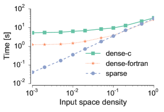
(a) Learning time

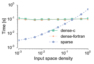
(b) Prediction time

Figure 8.2: Learning and prediction time of stumps as a function of the input space density.

Figure 8.3 shows the time required to learn a fully grown decision tree as a function of the dataset density. Note that the maximal depth decreases as a function of the dataset density (see Figure 8.3c) as the decision tree becomes more balanced. As with the stump, the fortran layout is more appropriate than the c layout to grow a fully grown decision tree on sparse data. The sparse csc algorithm is significantly faster than the dense splitting algorithm if the density is sufficiently low (here below $0.02$). The sparse splitting algorithm becomes slower as the density increases (here beyond $0.02$) since the extraction of the non zero values becomes more costly than finding the right split.

With fully developed decision trees, the prediction time (see Figure 8.3b) is similar between its dense and sparse version. The prediction time is lower when the input space density is high as the trees are more balanced. We note that the prediction time is correlated with the maximal depth of the tree.

Whenever the complexity of the decision tree lies between a stump and a fully developed tree, the behavior moves from one extreme to the other.

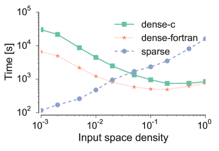
(a) Learning time

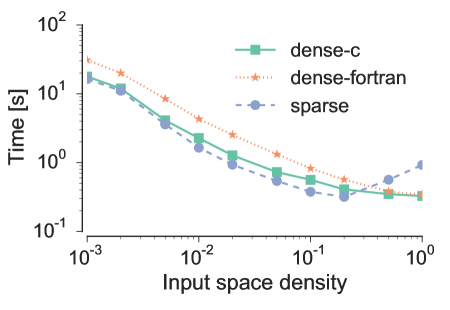
(b) Prediction time

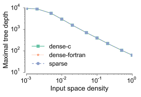
(c) Maximal depth

Figure 8.3: Learning time, prediction time and maximal depth as a function of the input space as a function of the input space density for fully grown decision trees.

30.2   Effect of the input space density on real datasets

To further study the impact of the input space density, we have selected 9 datasets whose input space density ranges from $0.00034$ to $0.22$. These datasets are presented in Table 8.1 ordered by input space density.

Table 8.1: Dataset properties ordered by input space density.

Dataset	n	p	Density
news20.binary Keerthi and DeCoste (2005)	19996	1355191	0.0003
20newsgroup Lang (1995); Rennie and Rifkin (2001)	11314	130107	0.0012
rcv1 Bekkerman and Scholz (2008)	23149	47236	0.0016
sector-scale Rennie and Rifkin (2001); Keerthi et al. (2008)	9619	55197	0.0029
farm-ads-vect Mesterharm and Pazzani (2011)	4143	54877	0.0036
E2006-train Kogan et al. (2009)	16087	150360	0.0083
mushrooms Lichman (2013)	8124	112	0.1875
mnist LeCun et al. (1998)	70000	784	0.1914
covtype Lichman (2013)	581012	54	0.2110

Table 8.2 shows the time to train a single stump. The fastest algorithm here is the tree growing algorithm with the input sparse csc matrix. The speed up factor between the sparse and fortran memory layout ranges from 1.1 to 23 times. Note that the fortran layout is always faster than the c layout. The column major order layout is here better suited for sparse dataset. The difference could be explained by fewer cache misses with the fortran memory layout than with the c memory layout.

Table 8.2: The time (in second) required to train a stump using a sparse csc layout is always faster than with the fortran or c dense memory layout on all sparse selected datasets.

Dataset	c	fortran	sparse	fortran / sparse
news20.binary	N/A	N/A	3.31	N/A
20newsgroup	213.18	15.77	0.79	20.1
rcv1	197.61	28.90	15.97	1.8
sector-scale	58.56	7.10	1.08	6.6
farm-ads-vect	26.03	3.22	0.14	23.0
E2006-train	413.35	35.44	8.62	4.1
mushrooms	0.03	0.02	0.02	1.2
mnist	5.23	2.65	2.00	1.3
covtype	3.89	2.57	2.35	1.1

Table 8.3 shows the time required to grow a fully developed decision tree with c, fortran or sparse csc memory layout. The dense fortran layout is here always faster than the dense c layout. The sparse memory layout is faster by a factor between 1.3 and 7.5 than the fortran layout when the input space density is below $0.3\%$.

Table 8.3: The time required to train a fully grown decision tree using a c, a fotran or a sparse csc memory layout.

Dataset	c	fortran	sparse	fortran / sparse
news20.binary	N/A	N/A	428.89	N/A
20newsgroup	4281.02	518.34	69.06	7.5
rcv1	1458.45	562.19	442.15	1.3
sector-scale	5337.65	878.67	206.69	4.3
farm-ads-vect	227.24	45.71	7.95	5.7
E2006-train	2467.39	752.15	1083.62	0.7
mushrooms	0.07	0.05	0.04	1.3
mnist	80.09	56.11	178.59	0.3
covtype	53.51	33.82	240.26	0.1

Note that we were unable to grow a decision tree with a dense memory layout on the news20.binary dataset as it would require 108.4 Gigabyte to only store the input matrix instead of 78 Megabytes.

30.3   Algorithm comparison on 20 newsgroup

Decision trees are rarely used in the context of sparse input datasets. One reason is the lack of implementations exploiting sparsity during the decision tree growth. With the previous experiments, we have shown that it increases significantly the computing time, but also the amount of memory needed. With the proposed tree growing and prediction algorithms, it is interesting to compare the training time, prediction time and accuracy of some tree based models, such as random forest or adaboost, with methods more commonly used in the presence of sparse data.

We compare tree based methods to methods more commonly used on sparse datasets on the 20 newsgroup dataset, which have $p=130107$ input variables, 11314 training sample ands 7532 testing samples.

The compared algorithms are optimized on their respective hyper-parameters (see Table 8.4 for the details) using 5-fold cross validation strategy on the training samples.

Table 8.4: Hyper-parameters grids.

$k$-nearest neighbors
$k$, number of neighbors	$\{1,\ldots,10\}$
Decision tree
$n_{\min}$, min. number of samples to split a node	$\{2,5,10,15\}$
Extra trees, random forest
$n_{\min}$, min. number of samples to split a node	$\{2,5,10,15\}$
$k$, number of features drawn at each nodes	$\{1,\log{p},\sqrt{p},0.001p\}$
$M$, ensemble size	100 or 1000
Adaboost with decision trees as weak estimators
$n_{\min}$, min. number of samples to split a node	$\{2,5,10,15\}$
$k$, number of features drawn at each nodes	$\{1,\log{p},\sqrt{p},0.001p\}$
$M$, ensemble size	100
$\mu$, learning rate	$\{1,0.1,0.01\}$
Bernoulli and multinomial naive Bayes
$\lambda$, additive smoothing parameter	$\{0,0.001,0.01,0.1,1\}$
Ridge classifier
$\lambda$, penalty parameter	$\{0.0001,0.001,0.01,0.1,1,10\}$
Linear support vector machine classifier (SVC)
$\lambda$, penalty parameter	$\{10^{i}\}_{i=-5}^{4}$
Stochastic gradient descent (SGD)
Loss	$\{\text{hinge},\text{logistic}\}$
Penalty constraint	$\{\ell_{1},\ell_{2},\text{elastic net}\}$
$\lambda$, penalty parameter	$\{0.0001,0.001,0.01,0.1,1,10\}$
Number of iterations	100

The results obtained on the 20 newsgroup dataset are shown in Table 8.5 using scikit-learn version 0.17.1 and input sparsity-aware implementations. The algorithm with the highest accuracy is the linear estimator trained with ridge regression. It is closely followed by the random forest ($m=1000$) model, the multinomial naives Bayes and extra-trees ($m=1000$). More generally, tree-based ensemble methods (random forest, extra trees, and adaboost) show similar performance as linear methods (ridge, naive bayes, linear SVC and SGD), with all methods from these two families reaching at least $0.75$ of accuracy. On the other hand, the $k$-nearest neighbors and the single decision tree perform very poorly (with an accuracy below $0.6$).

We also note that increasing the number of trees from 100 to 1000 significantly improves the performance of both random forests and extra trees. Their accuracy increases respectively by $0.0573$ and $0.0409$ in absolute value. Building tree ensembles also very significantly improves the accuracy with respect to single trees (by at least $0.20$). This further suggests that the variance of single trees is very high on this problem.

From a modeling perspective, growing decision tree ensemble on datasets with sparse inputs is possible. From a training time perspective, the time needed to grow and to optimize an ensemble of 100 trees is comparable to the time needed to train linear models, e.g., with SGD or ridge regression. Note that naive Bayes models are particularly fast to train compared to the other estimators. However note that the comparison is dependent upon the chosen hyper-parameters, the implementation and the grid size. From the point of view of prediction time, tree ensemble methods are particularly slow compared to the other estimators.

Table 8.5: Accuracy, training time (in second) and prediction time (in second) of algorithms on 20 newsgroup sorted by accuracy score.

Estimator	Training time	Prediction time	Accuracy
$K$-nearest neighbors	295	22.35	0.457
Decision tree	859	0.02	0.557
Adaboost	37867	8.84	0.752
Bernoulli naives Bayes	25	0.52	0.765
Random forest ($m=100$)	11766	12.71	0.778
Extra trees ($m=100$)	22186	28.07	0.794
SGD	42776	0.25	0.814
Linear SVC	2481	0.20	0.822
Extra trees ($m=1000$)	213009	253.39	0.833
Multinomial naives Bayes	14	0.11	0.833
Random forest ($m=1000$)	114472	125.92	0.835
Ridge	5737	0.13	0.844

31   Conclusion

We propose an algorithm to grow decision tree models whenever the input space is sparse. Our approach takes advantage of input sparsity to speed up the search and selection of the best splitting rule during the tree growing. It first speeds up the expansion of a tree node by extracting efficiently the non zero threshold of the splitting rules used to partition data. Secondly, the selection of best splitting rule is also faster as we avoid to sort data with zero values. We reduce the memory needed as we do not need to densify the input space. We also show how to predict samples with sparse inputs.

Conclusions

32   Conclusions

As we now gather or generate data at every moment, machine learning techniques are emerging as ubiquitous tools in sciences, engineering, or society. Within machine learning, this thesis focuses on supervised learning, which aims at modelling input-output relationships only from observations of input-output pairs, using tree-based ensemble methods, a popular method family exploiting tree structured input-output models. Modern applications of supervised learning raise new computational, memory, and modeling challenges to existing supervised learning algorithms. In this work, we identified and addressed the following questions in the context of tree-based supervised learning methods: (i) how to efficiently learn in high dimensional, and possibly sparse, output spaces? (ii) how to reduce the memory requirement of tree-based models at prediction time? (iii) how to efficiently learn in high dimensional and sparse input spaces? We summarize below our main contributions and conclusions around these three questions.

Learning in high dimensional and possibly sparse output spaces.

Decision trees are grown by recursively partitioning the input space while selecting at each node the split maximizing the reduction of some impurity measure. Impurity measures have been extended to address with such models multi-dimensional output spaces, so as to solve multi-label classification or multi-target regression problems. However, when the output space is of high dimension, the computation of the impurity becomes a computational bottleneck of the tree growing algorithm. To speed up this algorithm, we propose to approximate impurity computations during tree growing through random projections of the output space. More precisely, before growing a tree, a few random projections of the output space are computed and the tree is grown to fit these projections instead of the original outputs. Tree leaves are then relabelled in the original output space to provide proper predictions at test time. We show theoretically that when the number of projections is large enough, impurity scores, and thereby the learned tree structures and their predictions, are not affected by this trick. We then exploit the randomization introduced by the projections in the context of random forests, by building each tree of the forest from a different randomly projected subspace. Through experiments on several multi-label classification problems, we show that randomly projecting the outputs can significantly reduce computing times at training without affecting predictive performance. On some problems, the randomization induced by the projections even allows to reach a better bias-variance tradeoff within random forests, which leads to improved overall performance. In contrast with existing works on random projections of the output, our proposed leaf relabelling strategy also allows to avoid any decoding step and thus preserves computational efficiency at prediction time with respect to standard unprojected multi-output random forests.

Multi-output random forests build a single tree ensemble to predict all outputs simultaneously. While often effective, this approach is justified only when the individual outputs are strongly dependent (conditionally to the inputs). On the other hand, building a separate ensemble for each output, as done in the binary relevance / single target approach, is justified only when the outputs are (conditionally) independent. In our second contribution, we build on gradient boosting and random projections to propose a new approach that tries to bridge the gap between these two extreme assumptions and can hopefully adapt automatically to any intermediate output dependency structure. The idea of this approach is to grow each tree of a gradient boosting ensemble to fit a random projection of the original (residual) output space and then to weight this model in the prediction of each output according to its “correlation” with this output. Through extensive experiments on several artificial and real problems, we show that the resulting method has a faster convergence than binary relevance and that it can adapt better than both binary relevance and multi-output gradient boosting to any output dependency structure. The resulting method is also competitive with multi-output random forests. Although we only carried out experiments with tree-based weak models, the resulting gradient boosting methods are generic and can thus be used with any base regressor.

Reducing memory requirements of tree-based models at prediction time.

One drawback of random forest methods is that they need to grow very large ensembles of unpruned trees to achieve optimal performance. The resulting models are thus potentially very complex, especially with large datasets, as the complexity of unpruned trees typically depends linearly on the dataset size. On the other hand, only very few nodes are required to make a prediction for a given test example. Our investigation of the question of ensemble compression started with the observation that the random forest model can be viewed as linear models in the node indicator space. Each of these binary variables defining this space indicates whether or not a sample reaches a given node of the forest. In the original linear representation of a forest in the indicator space, non zero “coefficients” are given only to the leaf nodes. We propose to post-prune the random forest model by selecting and re-weighting the nodes of the linear model through the exploitation of sparse linear estimators. More precisely, from the tree ensemble, we first extract node indicator variables. Then, we project a sample set on this new representation and select a subset of these variables through a Lasso model. The non zero coefficients of the obtained Lasso model are later used to prune and to re-weight the decision tree structure. The resulting post-pruning approach is shown experimentally to reduce very significantly the size of random forests, while preserving, and even sometimes improving, their predictive performance.

Learning in high dimensional and sparse input spaces.

Some supervised learning tasks (e.g., text classification) need to deal with high dimensional and sparse input spaces, where input variables have each only a few non zero values. Dealing with input sparsity in the context of decision tree ensembles is challenging computationally for two reasons: (i) it is more difficult algorithmic-wise to exploit sparsity during the tree growth than for example with linear models, leading to slow tree training algorithms requiring a high amount of memory, (ii) the decision tree structures are very unbalanced, which further affects computational complexity. For these two reasons, linear methods are often preferred to decision tree algorithms to learn with sparse datasets. In our last contribution, we specifically developed an efficient implementation of the tree growing algorithm to handle sparse input variables. While previous implementations required to densify the input data matrix, our implementation allows to directly fit decision trees on appropriate sparse input matrices. It speeds up decision tree training on sparse input data and saves memory by avoiding input data “densification”. We also show how to predict unseen sparse input samples with a decision tree model. Note that in this contribution we only focus on improving computing times without modifying the original algorithm.

33   Perspectives and future works

We collect in this section some future research directions based on the presented ideas of this thesis.

33.1   Learning in compressed space through random projections

• The combination of random forest models with random projections adds two new hyper-parameters to tree based methods: the choice and the size of the random output projection subspace. It is not clear yet what would be good default hyper-parameter choices. Extensive empirical studies and the Johnson-Lindenstrauss lemma might help us to define good default values. These two hyper-parameters also introduce randomization in the output space. It would be interesting to further investigate how the input and output space randomizations jointly modify the bias-variance tradeoff of the ensemble.

• Single random projection of the output space with the gradient boosting algorithm is a generic multi-output method usable with any single output regressor. In this thesis, we specifically focused on tree-structured weak models. We suggest to investigate other kinds of weak models.

• We have combined a dimensionality reduction method with an ensemble method, random forest methods in Chapter 5 and with gradient boosting methods in Chapter 6, while keeping the generation of the random projection matrix independent from the supervised learning task. It would be interesting to investigate more adaptive projection schemes. A simple instance of this approach would be to draw a new random projection matrix according to the residuals, e.g. by sub-sampling an output variable with a probability proportional to the fraction of unexplained variance. An optimal instance of this approach, but computationally more expensive, would compute a projection maximizing the variance along each axis with the principal component analysis algorithm.

• Kernelizing the output of tree-based methods Geurts et al. (2006b, 2007) allows one to treat complex outputs such as images, texts and graphs. It would be interesting to investigate how to combine output kernel tree-based methods with random projection of the output space to improve computational complexity and accuracy. This idea has been studied Lopez-Paz et al. (2014) in the context of the kernel principal component algorithm and the kernel canonical correlation analysis algorithm.

33.2   Growing and compressing decision trees

• In the context of the $\ell_{1}$-based compression of random forests, we first grow a whole forest, and then prune it. The post-pruning step is costly in terms of computational time and memory as we start from a complex random forest model. A first study in collaboration with Jean-Michel Begon Begon et al. (2016) shows that we actually do not need to start from the whole forest, and can grow a compressed random forest model greedily. Starting from a set of root nodes, the idea is to sequentially develop the nodes that reduce the most the error of the chosen loss function. The process continues until reaching a complexity constraint, saving time and memory.

• The space complexity of a decision tree model is linear in the number of (test and leaf) nodes, which is typically proportional to the training set size $n$. In the context of $d$ outputs multi-output classification or regression tasks, or $d$ classes multi-class classification tasks, a leaf node is a constant model stored as a vector of size $d$. The space complexity of a decision tree model is thus $O(nd)$. With high dimensional output spaces or many classes, it thus may become prohibitive to store decision tree or random forest models. We would like to investigate two further approaches to compress such models: (i) by adapting the (post)-pruning method developed in Joly et al. (2012) and in Chapter 7 to multi-output tasks and multi-class classification tasks and (ii) by compressing exactly or approximately each constant leaf model. Both approaches can be used together. For approach (ii), an exact solution would compute the constant leaf models on-the-fly at prediction time by storing once the output matrix and the indices of the samples reaching the leaf at learning time. With totally developed trees, it should not modify the computational complexity of the prediction algorithm. If we agree to depart from the vanilla decision tree model, it is also possible to approximate the leaf model, for instance by keeping at the leaf nodes only the subset of the $k$ output-values reducing the most the error either at the leaf level as in Prabhu and Varma (2014) or at the tree level. Also, if the output space is sparse, appropriate sparse data structures could help to further reduce the memory footprint of the models.

33.3   Learning in high dimensional and sparse input-output spaces

• In Chapter 8, we have shown how to improve tree growing efficiency in the case of sparse high-dimensional input spaces. However, the small fraction of non zero input values exploited for each split typically leads to highly unbalanced tree structure. On such tasks, it would be interesting to grow decision trees with multivariate splitting rules to make the tree balanced. For instance in text-based supervised learning, the input text is often converted to a vector through a bag-of-words, where each variable indicates the presence of a single word. In this context, each test node assesses the presence or the absence of a single word. The tree growing algorithm lead to unbalanced trees as each training sample has only a small fraction of all possible words. We propose to investigate node splitting methods that would combine several sparse input variables into a dense one. In the text example, we would generate new dense variables by collapsing several words together. In a more general context, we could use random “or” or random “addition” functions of several sparse input variables.

  Furthermore, while we have shown empirically that the implementation proposed in Chapter  8 indeed translates into a speed up and reduction of memory consumption, it would be interesting to study formally its computational complexity as a function of the input-space sparsity.

• In the multi-label classification task, the output space is often very large and sparse (as in Chapter 5 and Chapter 6), having few “non zero values”. It would be interesting to exploit the output space sparsity to speed up the decision tree algorithm. The algorithm interacts with the output space during the search of the best split and the training of the leaf models. The search for the best split for an ordered variable is done by first sorting the possible splitting rules according to their threshold values, and then the best split is selected by computing incrementally the reduction of impurity by moving samples from the right partition to the left partition. The leaf models are constant estimators obtained by aggregating output values. Both procedures require efficient sample-wise indexing or row-wise indexing as provided by the compressed row storage (csr) sparse matrix format. We propose to implement impurity functions and leaf model training procedures to work with csr sparse matrices.

Part IV   Appendix

Description of the datasets

Appendix 10.A Synthetic datasets

• Friedman1 Friedman (1991) is a regression problem with $p=10$ independent input variables of uniform distribution $\mathcal{U}(0,1)$. We try to estimate the output $y=10\sin{(\pi{}\,x_{1}\,x_{2})}+20(x_{3}-\frac{1}{2})^{2}+10x_{4}+6x_{5}+\epsilon{}$, where $\epsilon$ is a Gaussian noise $\mathcal{N}(0,1)$. There are $300$ learning samples and $2000$ testing samples.

• Two-norm Breiman (1996b) is a binary classification problem with $p=20$ normally distributed (and class-conditionally independent) input variables: either from $\mathcal{N}(-a,1)$ if the class is $0$ or from $\mathcal{N}(a,1)$ if the class is 1 (with $a=\frac{2}{\sqrt{20}}$). There are $300$ learning and $2000$ testing samples.

Appendix 10.B Regression datasset

• SEFTi AA&YA (2008) is a (simulated) regression problem which concerns the tool level fault isolation in a semiconductor manufacturing. One quarter of the values are missing at random and were replaced by the median. There are $p=600$ input variables, $2000$ learning samples and $2000$ testing samples.

Appendix 10.C Multi-label dataset

Experiments are performed on several multi-label datasets: the yeast Elisseeff and Weston (2001) and the bird Briggs et al. (2013) datasets in the biology domain; the corel5k Duygulu et al. (2002) and the scene Boutell et al. (2004) datasets in the image domain; the emotions Tsoumakas et al. (2008b) and the CAL500 Turnbull et al. (2008) datasets in the music domain; the bibtex Katakis et al. (2008), the bookmarks Katakis et al. (2008), the delicious Tsoumakas et al. (2008a), the enron Klimt and Yang (2004), the EUR-Lex (subject matters, directory codes and eurovoc descriptors) Mencía and Fürnkranz (2010) the genbase Diplaris et al. (2005), the medical, the tmc2007 Srivastava and Zane-Ulman (2005) datasets in the text domain and the mediamill Snoek et al. (2006) dataset in the video domain.

Several hierarchical classification tasks are also studied to increase the diversity in the number of label and treated as multi-label classification task. Each node of the hierarchy is treated as one label. Nodes of the hierarchy which never occured in the training or testing set were removed. The reuters Rousu et al. (2005), WIPO Rousu et al. (2005) datasets are from the text domain. The Diatoms Dimitrovski et al. (2012) dataset is from the image domain. SCOP-GO Clare (2003), Yeast-GO Barutcuoglu et al. (2006) and Expression-GO Vens et al. (2008) are from the biological domain. Missing values in the Expression-GO dataset were inferred using the median for continuous features and the most frequent value for categorical features using the entire dataset. The inference of a drug-protein interaction network Yamanishi et al. (2011) is also considered either using the drugs to infer the interactions with the protein (drug-interaction), either using the proteins to infer the interactions with the drugs (protein-interaction).

Those datasets were selected to have a wide range of number of outputs $d$. Their basic characteristics are summarized at Table 10.1. For more information on a particular dataset, please see the relevant paper.

Table 10.1: Selected datasets have a number of labels $d$ ranging from 6 up to 3993 in the biology, the text, the image, the video or the music domain. Each dataset has $n_{LS}$ training samples, $n_{TS}$ testing samples and $p$ input features.

Datasets	$n_{LS}$	$n_{TS}$	$p$	$d$
emotions	391	202	72	6
scene	1211	1196	2407	6
yeast	1500	917	103	14
birds	322	323	260	19
tmc2007	21519	7077	49060	22
genbase	463	199	1186	27
reuters	2500	5000	19769	34
medical	333	645	1449	45
enron	1123	579	1001	53
mediamill	30993	12914	120	101
Yeast-GO	2310	1155	5930	132
bibtex	4880	2515	1836	159
CAL500	376	126	68	174
WIPO	1352	358	74435	188
EUR-Lex (subject matters)	19348	10-cv	5000	201
bookmarks	65892	21964	2150	208
diatoms	2065	1054	371	359
corel5k	4500	500	499	374
EUR-Lex (directory codes)	19348	10-cv	5000	412
SCOP-GO	6507	3336	2003	465
delicious	12920	3185	500	983
drug-interaction	1396	466	660	1554
protein-interaction	1165	389	876	1862
Expression-GO	2485	551	1288	2717
EUR-Lex (eurovoc descriptors)	19348	10-cv	5000	3993

Appendix 10.D Multi-output regression datasets

Multi-output regression is evaluated on several real world datasets: the edm Karalič and Bratko (1997) dataset in the industrial domain; the water-quality Džeroski et al. (2000) dataset in the environmental domain; the atp1d Spyromitros-Xioufis et al. (2016), the atp7d Spyromitros-Xioufis et al. (2016), the scm1d Spyromitros-Xioufis et al. (2016) and the scm20d Spyromitros-Xioufis et al. (2016) datasets in the price prediction domain; the oes97 Spyromitros-Xioufis et al. (2016) and the oes10 Spyromitros-Xioufis et al. (2016) datasets in the human resource domain. The output of those datasets were normalized to have zero mean and unit variance.

If the number of testing samples is unspecified, we use a $50\%$ of the samples as training and validation set and $50\%$ of the samples as testing set.

Table 10.2: Selected multi-output regression ranging from $d=2$ to $d=16$ outputs.

Datasets	$n_{LS}$	$n_{TS}$	$p$	$d$
atp1d	337		411	6
atp7d	296		411	6
edm	154		16	2
oes10	403		298	16
oes97	334		263	16
scm1d	8145	1658	280	16
scm20d	7463	1503	61	16
water-quality	1060		16	14

References

- AA&YA (2008) I. AA&YA. Manufacturing data: Semiconductor tool fault isolation, 11 2008. URL mailto:causality@clopinet.com.
- Achlioptas (2003) D. Achlioptas. Database-friendly random projections: Johnson-lindenstrauss with binary coins. Journal of computer and System Sciences, 66(4):671–687, 2003.
- Agrawal et al. (2013) R. Agrawal, A. Gupta, Y. Prabhu, and M. Varma. Multi-label learning with millions of labels: Recommending advertiser bid phrases for web pages. In Proceedings of the 22nd international conference on World Wide Web, pages 13–24. International World Wide Web Conferences Steering Committee, 2013.
- Airola et al. (2011) A. Airola, T. Pahikkala, W. Waegeman, B. De Baets, and T. Salakoski. An experimental comparison of cross-validation techniques for estimating the area under the roc curve. Computational Statistics & Data Analysis, 55(4):1828–1844, 2011.
- Almuallim (1996) H. Almuallim. An efficient algorithm for optimal pruning of decision trees. Artificial Intelligence, 83(2):347–362, 1996.
- Amit et al. (1997) Y. Amit, D. Geman, and K. Wilder. Joint induction of shape features and tree classifiers. Pattern Analysis and Machine Intelligence, IEEE Transactions on, 19(11):1300–1305, 1997.
- Bakker and Heskes (2003) B. Bakker and T. Heskes. Task clustering and gating for bayesian multitask learning. Journal of Machine Learning Research, 4(May):83–99, 2003.
- Baldassarre et al. (2012) L. Baldassarre, L. Rosasco, A. Barla, and A. Verri. Multi-output learning via spectral filtering. Machine Learning, 87(3):259–301, 2012.
- Barrett et al. (1994) R. Barrett, M. Berry, T. F. Chan, J. Demmel, J. Donato, J. Dongarra, V. Eijkhout, R. Pozo, C. Romine, and H. V. der Vorst. Templates for the Solution of Linear Systems: Building Blocks for Iterative Methods, 2nd Edition. SIAM, Philadelphia, PA, 1994.
- Barutcuoglu et al. (2006) Z. Barutcuoglu, R. E. Schapire, and O. G. Troyanskaya. Hierarchical multi-label prediction of gene function. Bioinformatics, 22(7):830–836, 2006.
- Bauer and Kohavi (1999) E. Bauer and R. Kohavi. An empirical comparison of voting classification algorithms: Bagging, boosting, and variants. Machine learning, 36(1-2):105–139, 1999.