A Framework for Algorithm Stability

Abstract.

We say that an algorithm is stable if small changes in the input result in small changes in the output. This kind of algorithm stability is particularly relevant when analyzing and visualizing time-varying data. Stability in general plays an important role in a wide variety of areas, such as numerical analysis, machine learning, and topology, but is poorly understood in the context of (combinatorial) algorithms.

In this paper we present a framework for analyzing the stability of algorithms. We focus in particular on the tradeoff between the stability of an algorithm and the quality of the solution it computes. Our framework allows for three types of stability analysis with increasing degrees of complexity: event stability, topological stability, and Lipschitz stability. We demonstrate the use of our stability framework by applying it to kinetic Euclidean minimum spanning trees.

1. Introduction

With recent advances in technology, vast amounts of time-varying data are being processed and analyzed on a daily basis. Time-varying data play an important role in a many different application areas, such as computer graphics, robotics, simulation, and visualization. There is a great need for algorithms that can operate efficiently on time-varying data and that can offer guarantees on the quality of the results. A specific relevant subset of time-varying data are motion data: geometric time-varying data. To deal with the challenges of motion data, Basch et al. [5] introduced the kinetic data structures (KDS) framework in 1999. Kinetic data structures are data structures that efficiently maintain a structure on a set of moving objects.

The performance of a particular algorithm is usually judged with respect to a variety of criteria, with the two most common being solution quality and running time. In the context of algorithms for time-varying data, a third important criterion is stability. Whenever analysis results on time-varying data need to be communicated to humans, for example via visual representations, it is important that these results are stable: small changes in the data result in small changes in the output. These changes in the output are continuous or discrete depending on the algorithm: graphs usually undergo discrete changes while a convex hull of moving points changes continuously. Sudden changes in the visual representation of data disrupt the mental map [25] of the user and prevent the recognition of temporal patterns. Stability also plays a role if changing the result is costly in practice, for example in physical network design, where frequent total overhauls of the network are simply infeasible.

The stability of algorithms or methods has been well-studied in a variety of research areas, such as numerical analysis [23, 10], machine learning [7], control systems [4], and topology [9, 11]. In contrast, the stability of combinatorial algorithms for time-varying data has received little attention in the theoretical computer science community so far. Here it is of particular interest to understand the tradeoffs between solution quality, running time, and stability. As an example, consider maintaining a minimum spanning tree of a set of moving points. If the points move, it might have to frequently change significantly. On the other hand, if we start with an MST for the input point set and then never change it combinatorially as the points move, the spanning tree we maintain is very stable – but over time it can devolve to a low quality and very long spanning tree.

Our goal, and the focus of this paper, is to understand the possible tradeoffs between solution quality and stability. This is in contrast to earlier work on stability in other research areas, such as the ones mentioned above, where stability is usually considered in isolation. Since there are currently no suitable tools available to formally analyze tradeoffs involving stability, we introduce a new analysis framework. We believe that there are many interesting and relevant questions to be solved in the general area of algorithmic stability analysis and we hope that our framework is a first meaningful step towards tackling them.

Results and organization. We present a framework to measure and analyze the stability of algorithms. As a first step, we limit ourselves to analyzing the tradeoff between stability and solution quality, omitting running time from consideration. Our framework allows for three types of stability analysis of increasing degrees of complexity: event stability, topological stability, and Lipschitz stability. It can be applied both to motion data and to more general time-varying data. We demonstrate the use of our stability framework by applying it to the problem of kinetic Euclidean minimum spanning trees (EMSTs). Some of our results for kinetic EMSTs are directly more widely applicable.

In Section 2 we give an overview of our framework for stability. In Sections 3, 4, and 5 we describe event stability, topological stability, and Lipschitz stability, respectively. In each of these sections we first describe the respective type of stability analysis in a generic setting, followed by specific results using that type of stability analysis on the kinetic EMST problem. In Section 6 we make some concluding remarks on our stability framework. Omitted proofs can be found in Appendix A.

Related work. Stability is a natural point of concern in more visual and applied research areas such as graph drawing, (geo-)visualization, and automated cartography. For example, in dynamic map labelling  [6, 19, 18, 28], the consistent dynamic labelling model allows a label to appear and disappear only once, making it very stable. There are very few theoretical results, with the noteworthy exception of so-called simultaneous embeddings [8, 15] in graph drawing, which can be seen as a very restricted model of stability. However, none of these results offer any real structural insight into the tradeoff between solution quality and stability.

In computational geometry there are a few results on the tradeoff between solution quality and stability. pecifically, Durocher and Kirkpatrick [durocher2006steiner] study the stability of centers of kinetic point sets, and define the notion of $\kappa$-stable center functions, which is closely related to our concept of Lipschitz stability. In later work [13] they consider the tradeoff between the solution quality of Euclidean $2$-centers and a bound on the velocity with which they can move. De Berg et al. [12] show similar results in the black-box KDS model. One can argue that the KDS framework [21] already indirectly considers stability in a limited form, namely as the number of external events. However, the goal of a KDS is typically to reduce the running time of the algorithm, and rarely to sacrifice the running time or quality of the results to reduce the number of external events.

Kinetic Euclidean minimum spanning trees and related structures have been studied extensively. Katoh et al. [24] proved an upper bound of $O(n^{3}2^{\alpha(n)})$ for the number of external events of EMSTs of $n$ linearly moving points, where $\alpha(n)$ is the inverse Ackermann function. Rahmati et al. [29] present a kinetic data structure for EMSTs in the plane that processes $O(n^{3}\beta_{2s+2}^{2}(n)\log n)$ events in the worst case, where $s$ is a measure for the complexity of the point trajectories and $\beta_{s}(n)$ is an extremely slow-growing function. The best known lower bound for external events of EMSTs in $d$ dimensions is $\Omega(n^{d})$ [27]. Since the EMST is a subset of the Delaunay triangulation, we can also consider to kinetically maintain the Delaunay triangulation instead. Fu and Lee [16], and Guibas et al. [22] show that the Delaunay triangulation undergoes $O(n^{2}\lambda_{s+2}(n))$ external events (near-cubic), where $\lambda_{s}(n)$ is the maximum length of an $(n,s)$-Davenport-Schinzel sequence [34]. On the other hand, the best lower bound for external events of the Delaunay triangulation is only $\Omega(n^{2})$ [34]. Rubin improves the upper bound to $O(n^{2+\varepsilon})$, for any $\varepsilon>0$, if the number of degenerate events is limited [32], or if the points move along a straight line with unit speed [33]). Agarwal et al. [1] also consider a more stable version of the Delaunay triangulation, which undergoes at most a nearly quadratic number of external events. However, external events for EMSTs do not necessarily coincide with external events of the Delaunay triangulation [30]. To further reduce the number of external events, we can consider approximations of the EMST, for example via spanners or well-separated pair decompositions [3]. However, kinetic $t$-spanners already undergo $\Omega(\frac{n^{2}}{t^{2}})$ external events [17]. Our stability framework allows us to reduce the number of external events even further and to still state something meaningful about the quality of the resulting EMSTs.

2. Stability framework

Intuitively, we can say that an algorithm is stable if small changes in the input lead to small changes in the output. More formally, we can formulate this concept generically as follows. Let $\Pi$ be an optimization problem that, given an input instance $I$ from a set $\mathcal{I}$, asks for a feasible solution $S$ from a set $\mathcal{S}$ that minimizes (or maximizes) some optimization function $f\colon\mathcal{I}\times\mathcal{S}\rightarrow\mathbb{R}$. An algorithm $\mathcal{A}$ for $\Pi$ can be seen as a function $\mathcal{A}\colon\mathcal{I}\rightarrow\mathcal{S}$. Similarly, the optimal solutions for $\Pi$ can be described by a function $\operatorname{OPT}\colon\mathcal{I}\rightarrow\mathcal{S}$. To define the stability of an algorithm, we need to quantify changes in the input instances and in the solutions. We can do so by imposing a metric on $\mathcal{I}$ and $\mathcal{S}$. Let $d_{\mathcal{I}}\colon\mathcal{I}\times\mathcal{I}\rightarrow\mathbb{R}_{\geq 0}$ be a metric for $\mathcal{I}$ and let $d_{\mathcal{S}}\colon\mathcal{S}\times\mathcal{S}\rightarrow\mathbb{R}_{\geq 0}$ be a metric for $\mathcal{S}$. We can then define the stability of an algorithm $\mathcal{A}\colon\mathcal{I}\rightarrow\mathcal{S}$ as follows.

$$\operatorname{St}(\mathcal{A})=\max_{I,I^{\prime}\in\mathcal{I}}\frac{d_{\mathcal{S}}(\mathcal{A}(I),\mathcal{A}(I^{\prime}))}{d_{\mathcal{I}}(I,I^{\prime})}$$ (1)

This definition for stability is closely related to that of the multiplicative distortion of metric embeddings, where $\mathcal{A}$ induces a metric embedding from the metric space $(\mathcal{I},d_{\mathcal{I}})$ into $(\mathcal{S},d_{\mathcal{S}})$. The lower the value for $\operatorname{St}(\mathcal{A})$, the more stable we consider the algorithm $\mathcal{A}$ to be. As with the distortion of metric embeddings, there are many other ways to define the stability of an algorithm given the metrics, but the above definition is sufficient for our purpose.

For many optimization problems, the function $\operatorname{OPT}$ may be very unstable. This suggests an interesting tradeoff between the stability of an algorithm and the solution quality. Unfortunately, the generic formulation of stability provided above is very unwieldy. It is not always clear how to define metrics $d_{\mathcal{I}}$ and $d_{\mathcal{S}}$ such that meaningful results can be derived. Additionally, it is not obvious how to deal with optimization problems with continuous input and discrete solutions, where the algorithm is inherently discontinuous, and thus the stability is unbounded by definition. Finally, analyses of this form are often very complex, and it is not straightforward to formulate a simplified version of the problem. In our framework we hence distinguish three types of stability analysis: event stability, topological stability, and Lipschitz stability.

Event stability follows the setting of kinetic data structures (KDS). That is, the input (a set of moving objects) changes continuously as a function over time. However, contrary to typical KDSs where a constraint is imposed on the solution quality, we aim to enforce the stability of the algorithm. For event stability we simply disallow the algorithm to change the solution too rapidly. Doing so directly is problematic, but we formalize this approach using the concept of $k$-optimal solutions. As a result, we can obtain a tradeoff between stability and quality that can be tuned by the parameter $k$. Note that event stability captures only how often the solution changes, but not how much the solution changes at each event.

Topological stability takes a first step towards the generic setup described above. However, instead of measuring the amount of change in the solution using a metric, we merely require the solution to behave continuously. To do so we only need to define a topology on the solution space $\mathcal{S}$ that captures stable behavior. Surprisingly, even though we completely ignore the amount of change in a single time step, this type of analysis still provides meaningful information on the tradeoff between solution quality and stability. In fact, the resulting tradeoff can be seen as a lower bound for any analysis involving metrics that follow the used topology.

Lipschitz stability finally captures the generic setup described above. As the name suggests, we require the algorithm to be Lipschitz continuous and we provide an upper bound on the Lipschitz constant, which is equivalent to $\operatorname{St}(\mathcal{A})$. We are then again interested in the quality of the solutions that can be obtained with any Lipschitz stable algorithm. Given the complexity of this type of analysis, a complete tradeoff for any value of the Lipschitz constant is typically out of reach, but some results may be obtained for values that are sufficiently small or large.

Remark. Our framework makes the assumption that an algorithm is a function $\mathcal{A}\colon\mathcal{I}\rightarrow\mathcal{S}$. However, in a kinetic setting this is not necessarily true, since the algorithm has history. More precisely, for some input instance $I$, a kinetic algorithm may produce different solutions for $I$ based on the instances processed earlier. We generally allow this behavior, and for event stability this behavior is even crucial. However, for the sake of simplicity, we will treat an algorithm as a function. We also generally assume in our analysis that the input is time-varying, that is, the input is a function over time, or follows a trajectory through the input space $\mathcal{I}$. Again, for the sake of simplicity, this is not always directly reflected in our definitions. Beyond that, we operate in the black-box model, in the sense that the algorithm does not know anything about future instances.

While these are the conditions under which we use our framework, it can be applied in a variety of algorithmic settings, such as streaming algorithms and algorithms with dynamic input.

3. Event stability

The simplest and most intuitive form of stability is event stability. Similarly to the number of external events in KDSs, event stability captures only how often the solution changes.

3.1. Event stability analysis

Let $\Pi$ be an optimization problem with a set of input instances $\mathcal{I}$, a set of solutions $\mathcal{S}$, and optimization function $f\colon\mathcal{I}\times\mathcal{S}\rightarrow\mathbb{R}$. Following the framework of kinetic data structures, we assume that the input instances include certain parameters that can change as a function of time. To apply the event stability analysis, we require that all solutions have a combinatorial description, that is, the solution description does not use the time-varying parameters of the input instance. We further require that every solution $S\in\mathcal{S}$ is feasible for every input instance $I\in\mathcal{I}$. This automatically disallows any insertions or deletions of elements. Note that an insertion or a deletion would typically force an event, and thus including this aspect in our stability analysis does not seem useful.

For example, in the setting of kinetic EMSTs, the input instances would consist of a fixed set of points. The coordinates of these points can then change as a function over time. A solution of the kinetic EMST problem consists of the combinatorial description of a tree graph on the set of input points. Note that every tree graph describes a feasible solution for any input instance, if we do not insist on any additional restrictions like, e.g., planarity. The minimization function $f$ then simply measures the total length of the tree, for which we do need to use the time-varying parameters of the problem instance.

Rather than directly restricting the quality of the solutions, we aim to restrict the stability of any algorithm. To that end, we introduce the concept of $k$-optimal solutions. Let $d_{\mathcal{I}}$ be a metric on the input instances, and let $\operatorname{OPT}\colon\mathcal{I}\rightarrow\mathcal{S}$ describe the optimal solutions. We say that a solution $S\in\mathcal{S}$ is $k$-optimal for an instance $I\in\mathcal{I}$ if there exists an input instance $I^{\prime}\in\mathcal{I}$ such that $f(I^{\prime},S)=f(I^{\prime},OPT(I^{\prime}))$ and $d_{\mathcal{I}}(I,I^{\prime})\leq k$. With this definition any optimal solution is always $0$-optimal. Note that this definition requires a form of normalization on the metric $d_{\mathcal{I}}$, similar to that of e.g. smoothed analysis [35]. We therefore require that there exists a constant $c$ such that every solution $S\in\mathcal{S}$ is $c$-optimal for every instance $I\in\mathcal{I}$. For technical reasons we require the latter condition to hold only for some time interval $[0,T]$ of interest.

Following the framework of kinetic data structures, we typically require the functions of the time-varying parameters to be well-behaved (e.g., polynomial functions), for otherwise we cannot derive meaningful bounds. The event stability analysis then considers two aspects. First, we analyze how often the solution needs to change to maintain a $k$-optimal solution for every point in time. Second, we analyze how well a $k$-optimal solution approximates an optimal solution. Typically we are not able to directly obtain good bounds on the approximation ratio, but given certain reasonable assumptions, good approximation bounds as a function of $k$ can be provided.

3.2. Event stability for EMSTs

Our input consists of a set of points $P=\{p_{1},\ldots,p_{n}\}$ where each point $p_{i}$ has a trajectory described by the function $x_{i}\colon[0,T]\rightarrow\mathbb{R}^{d}$. The goal is to maintain a combinatorial description of a short spanning tree on $P$ that does not change often. We generally assume that the functions $x_{i}$ are polynomials with bounded degree $s$.

To properly use the concept of $k$-optimal solutions, we first need to normalize the coordinates. We simply assume that $x_{i}(t)\in[0,1]^{d}$ for $t\in[0,T]$. This assumption may seem overly restrictive for kinetic point sets, but note that we are only interested in relative positions, and thus the frame of reference may move with the points. Next, we define the metric $d_{\mathcal{I}}$ along the trajectory as follows.

$$d_{\mathcal{I}}(t,t^{\prime})=\max_{i}\|x_{i}(t)-x_{i}(t^{\prime})\|$$ (2)

Note that this metric, and the resulting definition of $k$-optimal solutions, is not specific to EMSTs and can be used in general for problems with kinetic point sets as input. In our case $\|a-b\|$ denotes the distance between $a$ and $b$ in the (Euclidean) $\ell_{2}$ norm. Now let $OPT(t)$ be the EMST at time $t$. Then, by definition, $OPT(t)$ is $k$-optimal at time $t^{\prime}$ if $d_{\mathcal{I}}(t,t^{\prime})\leq k$. Our approach is now very simple: we compute the EMST and keep that solution as long as it is $k$-optimal, after which we compute the new EMST, and so forth. Below we analyze how often we need to recompute the EMST, and how well a $k$-optimal solution approximates the EMST.

Number of events. To derive an upper bound on the number of events, we first need to bound the speed of any point with a polynomial trajectory and bounded coordinates. For this we can use a classic result known as the Markov Brothers’ inequality.

Lemma 3.1 ([26]).

Let $h(t)$ be a polynomial with degree at most $s$ such that $h(t)\in[0,1]$ for $t\in[0,T]$, then $|h^{\prime}(t)|\leq s^{2}/T$ for all $t\in[0,T]$.

Lemma 3.2.

Let $P$ be a kinetic point set with polynomial trajectories $x_{i}(t)\in[0,1]^{d}$ ($t\in[0,T]$) of degree at most $s$, then we need only $O(\frac{s^{2}}{k})$ changes to maintain a $k$-optimal solution.

Proof 3.3.

By Lemma 3.1 the velocity of any point is at most $s^{2}/T$. Now assume that we have computed an optimal solution $S$ for some time $t$. The solution $S$ remains $k$-optimal until one of the points has moved at least $k$ units. Since the velocity of the points is bounded, this takes at least $\Delta t=kT/s^{2}$ time, at which point we can recompute the optimal solution. Since the total time interval is of length $T$, this can happen at most $T/\Delta t=s^{2}/k$ times.

Next we show that this upper bound is tight up to a factor of $s$, using Chebyshev polynomials of the first kind [31]. A Chebyshev polynomial of degree $s$ with range $[0,1]$ and domain $[0,T]$ will pass through the entire range exactly $s$ times.

Lemma 3.4.

Let $P$ be a kinetic point set with $n$ points with polynomial trajectories $x_{i}(t)\in[0,1]^{d}$ ($t\in[0,T]$) of degree at most $s$, then we need $\Omega(\min(\frac{s}{k},sn))$ changes in the worst case to maintain a $k$-optimal solution.

Proof 3.5.

We can restrict ourselves to $d=1$. Let $p_{1}$ move along a Chebyshev polynomial of degree $s$, and let the remaining points be stationary and placed equidistantly along the interval $[0,1]$. As soon as $p_{1}$ meets one of the other points, then $p_{1}$ can travel at most $k$ units before the solution is no longer $k$-optimal (see Fig.1). Therefore, $p_{1}$ moving through the entire interval requires $\Omega(\min(1/k,n))$ changes to the solution. Doing so $s$ times gives the desired bound.

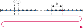
Figure 1. An instance where $\Omega(\frac{s}{k})$ events are triggered. The blue points are stationary, while the red point moves along a trajectory of degree $3$. The trajectory is shown as an arrow along the 1D space, where the gray part has already been traversed.

It is important to notice that this behavior is fairly special for polynomial trajectories. If we allow more general trajectories, then this bound on the number of changes breaks down.

Lemma 3.6.

Let $P$ be a kinetic point set with $n$ points with pseudo-algebraic trajectories $x_{i}(t)\in[0,1]^{d}$ ($t\in[0,T]$) of degree at most $s$, then we need $\Omega(\min(\frac{sn}{k},sn^{2}))$ changes in the worst case to maintain a $k$-optimal solution.

Proof 3.7.

We can restrict ourselves to $d=1$. Any two pseudo-algebraic trajectories of degree at most $s$ can cross each other at most $s$ times. We make $n/2$ points stationary and place them equidistantly along the interval $[0,1]$. The other $n/2$ points follow trajectories that take them through the entire interval $s$ times, in such a way that every point moves through the entire interval completely before another point does so. The resulting trajectories are clearly pseudo-algebraic, and each time a point moves through the entire interval it requires $\Omega(\min(1/k,n))$ changes to the solution. As a result, the total number of changes is $\Omega(\min(\frac{sn}{k},sn^{2}))$.

We can show the same lower bound for algebraic trajectories of degree at most $s$, but this is slightly more involved. The result can be found in Appendix A.

Approximation factor. We cannot expect $k$-optimal solutions to be a good approximation of optimal EMSTs in general: if all points are within distance $k$ from each other, then all solutions are $k$-optimal. We therefore need to make the assumption that the points are spread out reasonably throughout the motion. To quantify this, we use a measure inspired by the order-$l$ spread, as defined in [14]. Let be the smallest distance in $P$ between a point and its $l$-th nearest neighbor. We assume that throughout the motion, for some value of $\Delta_{l}$. We can use this assumption to give a lower bound on the length of the EMST. Pick an arbitrary point and remove all points from $P$ that are within distance $1/\Delta_{l}$, and repeat this process until the smallest distance is at least $1/\Delta_{l}$. By our assumption, we remove at most $l-1$ points for each chosen point, so we are left with at least $n/l$ points. The length of the EMST on P is at least the length of the EMST on the remaining $n/l$ points, which has length $\Omega(\frac{n}{l\Delta_{l}})$.

Lemma 3.8.

A $k$-optimal solution of the EMST problem on a set of $n$ points $P$ is an $O(1+kl\Delta_{l})$-approximation of the EMST, under the assumption that .

Proof 3.9.

Let $S$ be a $k$-optimal solution of $P$ and let $\operatorname{OPT}$ be an optimal solution of $P$. By definition there is a point set $P^{\prime}$ for which the length of solution $S$ is at most that of $\operatorname{OPT}$. Since $d_{\mathcal{I}}(P,P^{\prime})\leq k$, the length of each edge can grow or shrink by at most $2k$ when moving from $P^{\prime}$ to $P$. Therefore we can state that $f(P,S)\leq f(P,\operatorname{OPT})+4kn$. Now, using the lower bound on the length of an EMST, we obtain the following.

$$f(P,\operatorname{OPT})+4kn \leq f(P,\operatorname{OPT})+4kO(f(P,\operatorname{OPT})l\Delta_{l})$$

$$=O(1+kl\Delta_{l})\cdot f(P,\operatorname{OPT})$$

Note that there is a clear tradeoff between the approximation ratio and how restrictive the assumption on the spread is. Regardless, we can obtain a decent approximation while only processing a small number of events. If we choose reasonable values $k=O(1/n)$, $l=O(1)$, and $\Delta_{l}=O(n)$, then our results show that, under the assumptions, a constant-factor approximation of the EMST can be maintained while processing only $O(n)$ events.

4. Topological stability

The event stability analysis has two major drawbacks: (1) it is only applicable to problems for which the solutions are always feasible and described combinatorially, and (2) it does not distinguish between small and large structural changes. Topological stability analysis is applicable to a wide variety of problems and enforces continuous changes to the solution.

4.1. Topological stability analysis

Let $\Pi$ be an optimization problem with input instances $\mathcal{I}$, solutions $\mathcal{S}$, and optimization function $f$. An algorithm $\mathcal{A}\colon\mathcal{I}\rightarrow\mathcal{S}$ is topologically stable if, for any (continuous) path $\pi\colon[0,1]\rightarrow\mathcal{I}$ in $\mathcal{I}$, $\mathcal{A}\pi$ is a (continuous) path in $\mathcal{S}$. To properly define a (continuous) path in $\mathcal{I}$ and $\mathcal{S}$ we need to specify a topology $\mathcal{T}_{\mathcal{I}}$ on $\mathcal{I}$ and a topology $\mathcal{T}_{\mathcal{S}}$ on $\mathcal{S}$. Alternatively we could specify metrics $d_{\mathcal{I}}$ and $d_{\mathcal{S}}$, but this is typically more involved. We then want to analyze the approximation ratio of any topologically stable algorithm with respect to $\operatorname{OPT}$. That is, we are interested in the ratio

$$\operatorname{TS}(\Pi,\mathcal{T}_{\mathcal{I}},\mathcal{T}_{\mathcal{S}})=\inf_{\mathcal{A}}\sup_{I\in\mathcal{I}}\frac{f(I,\mathcal{A}(I))}{f(I,\operatorname{OPT}(I))}$$ (3)

where the infimum is taken over all topologically stable algorithms. Naturally, if $\operatorname{OPT}$ is already topologically stable, then this type of analysis does not provide any insight and the ratio is simply $1$. However, in many cases, $\operatorname{OPT}$ is not topologically stable. The above analysis can also be applied if the solution space (or the input space) is discrete. In such cases, continuity can often be defined using the graph topology of so-called flip graphs, for example, based on edge flips for triangulations or rotations in rooted binary trees. We can represent a graph as a topological space by representing vertices by points, and representing every edge of the graph by a copy of the unit interval $[0,1]$. These intervals are glued together at the vertices. In other words, we consider the corresponding simplicial $1$-complex. Although the points in the interior of the edges of this topological space do not represent proper spanning trees, we can still use this topological space in Equation LABEL:eq:topo by extending $f$ over the edges via linear interpolation. It is not hard to see that we need to consider only the vertices of the flip graph (which represent proper spanning trees) to compute the topological stability ratio.

4.2. Topological stability of EMSTs

We use the same setting of the kinetic EMST problem as in Section 3.2, except that we do not restrict the trajectories of the points and we do not normalize the coordinates. We merely require that the trajectories are continuous. To define this properly, we need to define a topology on the input space, but for a kinetic point set with $n$ points in $d$ dimensions we can simply use the standard topology on $\mathbb{R}^{dn}$ as $\mathcal{T}_{\mathcal{I}}$. To apply topological stability analysis, we also need to specify a topology on the (discrete) solution space. As the points move, the minimum spanning tree may have to change at some point in time by removing one edge and inserting another edge. Since these two edges may be very far apart, we do not consider this operation to be stable or continuous. Instead we specify the topology of $\mathcal{S}$ using a flip graph, where the operations are either edge slides or edge rotations [2, 20]. The optimization function $f$, measuring the quality of the EMST, is naturally defined for the vertices of the flip graph as the length of the spanning tree, and we use linear interpolation to define $f$ on the edges of the flip graph. For edge slides and rotations we provide upper and lower bounds on $\operatorname{TS}(\text{EMST},\mathcal{T}_{\mathcal{I}},\mathcal{T}_{\mathcal{S}})$.

Edge slides. An edge slide is defined as the operation of moving one endpoint of an edge to one of its neighboring vertices along the edge to that neighbor. More formally, an edge $(u,v)$ in the tree can be replaced by $(u,w)$ if $w$ is a neighbor of $v$ and $w\neq u$. Since this operation is very local, we consider it to be stable. Note that after every edge slide the tree must still be connected.

Lemma 4.1.

If $\mathcal{T}_{\mathcal{S}}$ is the topology on $\mathcal{S}$ defined by edge slides, then $\operatorname{TS}(\text{EMST},\mathcal{T}_{\mathcal{I}},\mathcal{T}_{\mathcal{S}})\leq\frac{3}{2}$.

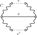
Figure 2. $x$ is the longest edge during an edge slide from $e$ to $e^{\prime}$.

Proof. Consider a point in time where the EMST has to be updated by removing an edge $e$ and inserting an edge $e^{\prime}$, where $|e|=|e^{\prime}|$. Note that $e$ and $e^{\prime}$ form a cycle $C$ with other edges of the EMST. We now slide edge $e$ to edge $e^{\prime}$ by sliding it along the vertices of $C$. Let $x$ be the longest intermediate edge when sliding from $e$ to $e^{\prime}$ (see Fig. 2). To allow $x$ to be as long as possible with respect to the length of the EMST, the EMST should be fully contained in $C$. By the triangle inequality we get that $2|x|\leq|C|$. Since the length of the EMST is $\operatorname{OPT}=|C|-|e|$, we get that $|x|\leq\operatorname{OPT}/2+|e|/2$. Thus, the length of the intermediate tree is $|C|-2|e|+|x|=\operatorname{OPT}-|e|+|x|\leq\frac{3}{2}\operatorname{OPT}$. ∎

Figure 3. This configuration is a $(\frac{\pi+1}{\pi}-\varepsilon)$-approximation of the EMST. (a) While $e$ slides to $e^{\prime}$ it becomes the diameter of the circle. (b) Stretching an edge $f$ to form a chord creates an even longer spanning tree.

Lemma 4.2.

If $\mathcal{T}_{\mathcal{S}}$ is the topology on $\mathcal{S}$ defined by edge slides, then, for any $\varepsilon>0$, $\operatorname{TS}(\text{EMST},\mathcal{T}_{\mathcal{I}},\mathcal{T}_{\mathcal{S}})\geq\frac{\pi+1}{\pi}-\varepsilon$.

Proof 4.3.

Consider a point in time where the EMST has to be updated by removing an edge $e$ and inserting an edge $e^{\prime}$, where $|e|$ is very small. Let the remaining points be arranged in a circle, as shown in Figure 3(a), such that the farthest distance between any two points is $\operatorname{OPT}/\pi-\varepsilon$, where $\operatorname{OPT}$ is the length of the EMST. We can make this construction for any $\varepsilon>0$ by using enough points and making $e$ and $e^{\prime}$ arbitrarily short. Simply sliding $e$ to $e^{\prime}$ will always grow $e$ to be the diameter of the circle at some point. Alternatively, $e$ can take a shortcut by sliding over another edge $f$ as a chord (see Figure 3(b)). This is only beneficial if $|e|+|f|<\operatorname{OPT}/\pi-\varepsilon$. However, if $f$ helps $e$ to avoid becoming a diameter of the circle, then $e$ and $f$, as chords, must span an angle larger than $\pi$ together. As a result, $|e|+|f|\geq\operatorname{OPT}/\pi-\varepsilon$ by triangle inequality.

A motion of the points that forces $e$ to slide to $e^{\prime}$ in this particular configuration looks as follows. The points start at $e$ and move at constant speed along the circle, half of the points clockwise and the other half counter clockwise. The speeds are assigned in such a way that at some point all points are evenly spread along the circle. Once all points are evenly spread, they start moving towards $e^{\prime}$, again along the circle. It is easy to see that, using the arguments above, any additional edges inside the circle must have total length of at least the diameter of the circle at some point throughout the motion. On the other hand, $\operatorname{OPT}$ is largest when the points are evenly spread along the circle. Thus, for any $\varepsilon>0$, $\operatorname{TS}(\text{EMST},\mathcal{T}_{\mathcal{I}},\mathcal{T}_{\mathcal{S}})\geq\frac{\pi+1}{\pi}-\varepsilon\approx 1.318-\varepsilon$.

Edge rotations. Edge rotations are a generalization of edge slides, that allow one endpoint of an edge to move to any other vertex. These operations are clearly not as stable as edge slides, but they are still more stable than the deletion and insertion of arbitrary edges.

Figure 4. If one part of $C$ is small enough, then we can rotate one endpoint of $e$ directly to one endpoint of $e^{\prime}$.

Figure 5. The potential intermediate edges when rotating edge $e$ to $e^{\prime}$.

Lemma 4.4.

If $\mathcal{T}_{\mathcal{S}}$ is the topology on $\mathcal{S}$ defined by edge rotations, then $\operatorname{TS}(\text{EMST},\mathcal{T}_{\mathcal{I}},\mathcal{T}_{\mathcal{S}})\leq\frac{4}{3}$.

Proof 4.5.

Consider a point in time where the EMST has to be updated by removing an edge $e=(u,v)$ and inserting an edge $e^{\prime}=(u^{\prime},v^{\prime})$, where $|e|=|e^{\prime}|$. Note that $e$ and $e^{\prime}$ form a cycle $C$ with other edges of the EMST. We now rotate edge $e$ to edge $e^{\prime}$ along some of the vertices of $C$. Let $x$ be the longest intermediate edge when rotating from $e$ to $e^{\prime}$. To allow $x$ to be as long as possible with respect to the length of the EMST, the EMST should be fully contained in $C$. We argue that $|x|\leq\operatorname{OPT}/3+|e|$, where $\operatorname{OPT}$ is the length of the EMST. Removing $e$ and $e^{\prime}$ from $C$ will split $C$ into two parts, where we assume that $u$ and $u^{\prime}$ ($v$ and $v^{\prime}$) are in the left (right) part. First assume that one of the two parts has length at most $\operatorname{OPT}/3$. Then we can rotate $e$ to $(u,v^{\prime})$, and then to $e^{\prime}$, which implies that $|x|=|(u,v^{\prime})|\leq\operatorname{OPT}/3+|e|$ by the triangle inequality (see Fig. 5). Now assume that both parts have length at least $\operatorname{OPT}/3$. Let $e_{L}=(u_{L},v_{L})$ be the edge in the left part that contains the midpoint of that part, and let $e_{R}=(u_{R},v_{R})$ be the edge in the right part that contains the midpoint of that part, where $u_{L}$ and $u_{R}$ are closest to $e$ (see Fig. 5). Furthermore, let $Z$ be the length of $C\setminus\{e,e^{\prime},e_{L},e_{R}\}$. Now consider the potential edges $(u,v_{R})$, $(v,v_{L})$, $(u^{\prime},u_{R})$, and $(v^{\prime},u_{L})$. By the triangle inequality, the sum of the lengths of these edges is at most $4|e|+2|e_{L}|+2|e_{R}|+Z$. Thus, one of these potential edges has length at most $|e|+|e_{L}|/2+|e_{R}|/2+Z/4$. Without loss of generality let $(u,v_{R})$ be that edge (the construction is fully symmetric). We can now rotate $e$ to $(u,v_{R})$, then to $(u^{\prime},v_{R})$, and finally to $e^{\prime}$. As each part of $C$ has length at most $2\operatorname{OPT}/3$, we get that $|(u^{\prime},v_{R})|\leq\operatorname{OPT}/3+|e|$ by construction. Furthermore we have that $\operatorname{OPT}=|e|+|e_{L}|+|e_{R}|+Z$. Thus, $|(u,v_{R})|\leq|e|+|e_{L}|/2+|e_{R}|/2+Z/4=\operatorname{OPT}/3+2|e|/3+|e_{L}|/6+|e_{R}|/6-Z/12$. Since $e$ needs to be removed to update the EMST, it must be the longest edge in $C$. Therefore $|(u,v_{R})|\leq\operatorname{OPT}/3+|e|$, which shows that $|x|\leq\operatorname{OPT}/3+|e|$. Since the length of the intermediate tree is $\operatorname{OPT}-|e|+|x|\leq\frac{4}{3}\operatorname{OPT}$, we obtain that $\operatorname{TS}(\text{EMST},\mathcal{T}_{\mathcal{I}},\mathcal{T}_{\mathcal{S}})\leq\frac{4}{3}$.

Lemma 4.6.

If $\mathcal{T}_{\mathcal{S}}$ is defined by edge rotations, then, $\operatorname{TS}(\text{EMST},\mathcal{T}_{\mathcal{I}},\mathcal{T}_{\mathcal{S}})\geq\frac{10-2\sqrt{2}}{9-2\sqrt{2}}$.

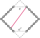
Figure 6. Lower bound construction for edge rotations.

Proof. Consider a point in time where the EMST has to be updated by removing an edge $e$ and inserting an edge $e^{\prime}$. Let the remaining points be arranged in a diamond shape as shown in Figure 6, where the side length of the diamond is $2$, and $|e|=|e^{\prime}|=1$. As a result, the distance between an endpoint of $e$ and the left or right corner of the diamond is $2-\frac{1}{2}\sqrt{2}$. Now we define a top-connector as an edge that intersects the vertical diagonal of the diamond, but is completely above the horizontal diagonal of the diamond. A bottom-connector is defined analogously, but must be completely below the horizontal diagonal. Finally, a cross-connector is an edge that crosses or touches both diagonals of the diamond. Note that a cross-connector has length at least $2$, and a top- or bottom-connector has length at least $|e|=1$. In the considered update, we start with a top-connector and end with a bottom-connector. Since we cannot rotate from a top-connector to a bottom-connector in one step, we must reach a state that either has both a top-connector and a bottom-connector, or a single cross-connector. In both options the length of the spanning tree is $10-2\sqrt{2}$, while the minimum spanning tree has length $9-2\sqrt{2}$.

To force the update from $e$ to $e^{\prime}$ in this configuration, we can use the following motion. The points start at the endpoints of $e$ and move with constant speeds to a position where the points are evenly spread around the left and right corner of the diamond. Then the points move with constant speeds to the endpoints of $e^{\prime}$. The argument above still implies that we need edges of total length at least $2$ intersecting the vertical diagonal of the diamond at some point during the motion. On the other hand, $OPT\leq 9-2\sqrt{2}$ throughout the motion. Thus $\operatorname{TS}(\text{EMST},\mathcal{T}_{\mathcal{I}},\mathcal{T}_{\mathcal{S}})\geq\frac{10-2\sqrt{2}}{9-2\sqrt{2}}\approx 1.162$.  ∎

5. Lipschitz stability

The major drawback of topological stability analysis is that it still does not fully capture stable behavior; the algorithm must be continuous, but we can still make many changes to the solution in an arbitrarily small time step. In Lipschitz stability analysis we additionally limit how fast the solution can change.

5.1. Lipschitz stability analysis

Let $\Pi$ be an optimization problem with input instances $\mathcal{I}$, solutions $\mathcal{S}$, and optimization function $f$. To quantify how fast a solution changes as the input changes, we need to specify metrics $d_{\mathcal{I}}$ and $d_{\mathcal{S}}$ on $\mathcal{I}$ and $\mathcal{S}$, respectively. An algorithm $\mathcal{A}\colon\mathcal{I}\rightarrow\mathcal{S}$ is $K$-Lipschitz stable if for any $I,I^{\prime}\in\mathcal{I}$ we have that $d_{\mathcal{S}}(\mathcal{A}(I),\mathcal{A}(I^{\prime}))\leq Kd_{\mathcal{I}}(I,I^{\prime})$. We are then again interested in the approximation ratio of any $K$-Lipschitz stable algorithm with respect to $\operatorname{OPT}$. That is, we are interested in the ratio

$$\operatorname{LS}(\Pi,K,d_{\mathcal{I}},d_{\mathcal{S}})=\inf_{\mathcal{A}}\sup_{I\in\mathcal{I}}\frac{f(I,\mathcal{A}(I))}{f(I,\operatorname{OPT}(I))}$$ (4)

where the infimum is taken over all $K$-Lipschitz stable algorithms. It is easy to see that $\operatorname{LS}(\Pi,K,d_{\mathcal{I}},d_{\mathcal{S}})$ is lower bounded by $\operatorname{TS}(\Pi,\mathcal{T}_{\mathcal{I}},\mathcal{T}_{\mathcal{S}})$ for the corresponding topologies $\mathcal{T}_{\mathcal{I}}$ and $\mathcal{T}_{\mathcal{S}}$ of $d_{\mathcal{I}}$ and $d_{\mathcal{S}}$, respectively. As already mentioned in Section 2, analyses of this type are often quite hard. First, we often need to be very careful when choosing the metrics $d_{\mathcal{I}}$ and $d_{\mathcal{S}}$, as they should behave similarly with respect to scale. For example, let the input consist of a set of points in the plane and let $cI$ for $I\in\mathcal{I}$ be the instance obtained by scaling all coordinates of the points in $I$ by the factor $c$. Now assume that $d_{\mathcal{I}}$ depends linearly on scale, that is $d_{\mathcal{I}}(cI,cI^{\prime})\sim cd_{\mathcal{I}}(I,I^{\prime})$, and that $d_{\mathcal{S}}$ is independent of scale. Then, for some fixed $K$, we can reduce the effective speed of any $K$-Lipschitz stable algorithm arbitrarily by scaling down the instances sufficiently, rendering the analysis meaningless. We further need to be careful with discrete solution spaces. However, using the flip graphs as mentioned in Section 4 we can extend a discrete solution space to a continuous space by including the edges.

Typically it will be hard to fully describe $\operatorname{LS}(\Pi,K,d_{\mathcal{I}},d_{\mathcal{S}})$ as a function of $K$. However, it may be possible to obtain interesting results for certain values of $K$. One value of interest is the value of $K$ from which the approximation ratio equals or approaches the approximation ratio of the corresponding topological stability analysis. Another potential value of interest is the value of $K$ below which any $K$-Lipschitz stable algorithm performs asymptotically as bad as a constant algorithm always computing the same solution regardless of instance.

5.2. Lipschitz stability of EMSTs

We use the same setting of the kinetic EMST problem as in Section 4.2, except that, instead of topologies, we specify metrics for $\mathcal{I}$ and $\mathcal{S}$. For $d_{\mathcal{I}}$ we can simply use the metric in Equation 2, which implies that points move with a bounded speed. For $d_{\mathcal{S}}$ we use a metric inspired by the edge slides of Section 4.2. To that end, we need to define how long a particular edge slide takes, or equivalently, how “far” an edge slide is. To make sure that $d_{\mathcal{I}}$ and $d_{\mathcal{S}}$ behave similarly with respect to scale, we let $d_{\mathcal{S}}$ measure the distance the sliding endpoint has traveled during an edge slide. However, this creates an interesting problem: the edge on which the endpoint is sliding may be moving and stretching/shrinking during the operation (see Fig. 7). This influences how long it takes to perform the edge slide. We need to be more specific: (1) As the points are moving, the relative position (between $0$ and $1$ from starting endpoint to finishing endpoint) of a sliding endpoint is maintained without cost in $d_{\mathcal{S}}$, and (2) $d_{\mathcal{S}}$ measures the difference in relative position multiplied by the length $L(t)$ of the edge on which the endpoint is sliding. More tangibly, an edge slide performed by a $K$-Lipschitz stable algorithm can be performed in $t^{*}$ time such that $\int_{0}^{t^{*}}\frac{K}{L(t)}\mathrm{d}t=1$, where $L(t)$ describes the length of the edge on which the endpoint slides as a function of time. Finally, the optimization function $f$ simply computes a linear interpolation of the cost on the edges of the flip graph defined by edge slides.

We now give an upper bound on $K$ below which any $K$-Lipschitz stable algorithm for kinetic EMST performs asymptotically as bad as any fixed tree. Given the complexity of the problem, our bound is fairly crude. We provide it anyway to demonstrate the use of our framework, but we believe that a stronger bound exists. First we show the asymptotic approximation ratio of any spanning tree.

Lemma 5.1.

Any spanning tree on a set of $n$ points $P$ is an $O(n)$-approximation of the EMST.

Lemma 5.2.

Let $d_{\mathcal{S}}$ be the metric for edge slides, then $\operatorname{LS}(\text{EMST},\frac{c}{\log n},d_{\mathcal{I}},d_{\mathcal{S}})=\Omega(n)$ for a small enough constant $c>0$, where $n$ is the number of points.

Proof 5.3.

Consider the instance where $n$ points are placed equidistantly vertically above each other with distance $1/n$ between two consecutive points. Now let $\mathcal{A}$ be any $(c/\log n)$-Lipschitz stable algorithm for the kinetic EMST problem and let $T$ be the tree computed by $\mathcal{A}$ on this point set. We now color the points red and blue based on a $2$-coloring of $T$. We then move the red points to the left by $\frac{1}{2}$ and the blue points to the right by $\frac{1}{2}$ in the time interval $[0,1]$ (see Fig. 7 left). This way every edge of $T$ will be stretched to a length of $\Omega(1)$ and thus the length of $T$ will be $\Omega(n)$. On the other hand, the length of the EMST in the final configuration is $\operatorname{OPT}=O(1)$. Therefore, we must perform an edge slide (see Fig. 7 middle). However, we show that $\mathcal{A}$ cannot complete any edge slide. Consider any edge of $T$ and let $x$ be the initial (vertical) distance between its endpoints. Then the length of this edge can be described as $L(t)=\sqrt{x^{2}+t^{2}}$ (see Fig. 7 right). Now assume that we want to slide an endpoint over this edge. To finish this edge slide before $t=1$, we require that $\int_{0}^{1}\frac{c}{\log n\sqrt{x^{2}+t^{2}}}\mathrm{d}t\geq 1$. This solves to $c\log(1/x+\sqrt{1+1/x^{2}})\geq\log n$. However, since $x\geq 1/n$, we get that $c\log(1/x+\sqrt{1+1/x^{2}})\leq c\log(n+\sqrt{1+n^{2}})<\log n$ for $c$ small enough. Finally, since one edge slide can reduce the length of only one edge to $o(1)$, the cost of the solution at $t=1$ computed by $\mathcal{A}$ is $\Omega(n)$. Thus, $\operatorname{LS}(\text{EMST},\frac{c}{\log n},d_{\mathcal{I}},d_{\mathcal{S}})=\Omega(n)$ for a small enough constant $c>0$.

Figure 7. An instance where any $K$-Lipschitz stable algorithm performs badly: Starting from a solution on equidistantly placed points, the red and blue points move in opposite directions (left). The endpoint of the red edge slides over stretching edge $T$ (middle). The length of edge $T$ at time $t$ is $\sqrt{x^{2}+t^{2}}$ (right).

6. Conclusion

We presented a framework for algorithm stability, which includes three types of stability analysis, namely event stability, topological stability, and Lipschitz stability. We also demonstrated the use of this framework by applying the different types of analysis to the kinetic EMST problem, deriving new interesting results. We believe that, by providing different types of stability analysis with increasing degrees of complexity, we make stability analysis for algorithms more accessible, and make it easier to formulate interesting open problems with regard to algorithm stability.

However, the framework that we have presented is not designed to offer a complete picture on algorithm stability. In particular, we do not consider the algorithmic aspect of stability. For example, if we already know how the input will change over time, can we efficiently compute a stable function of solutions over time that is optimal with regard to solution quality? Or, in a more restricted sense, can we efficiently compute the one solution that is best for all inputs over time? Even in the black-box model we can consider designing efficient algorithms that are $K$-Lipschitz stable and perform well with regard to solution quality. We leave such problems for future work.

Acknowledgements. W. Meulemans and J. Wulms are (partially) supported by the Netherlands eScience Center (NLeSC) under grant number 027.015.G02. B. Speckmann and K. Verbeek are supported by the Netherlands Organisation for Scientific Research (NWO) under project no. 639.023.208 and no. 639.021.541, respectively.

Appendix A Omitted proofs

Lemma A.1.

Let $P$ be a kinetic point set with $n$ points with algebraic trajectories $x_{i}(t)\in[0,1]^{d}$ ($t\in[0,T]$) of degree at most $s$, then we need $\Omega(\min(\frac{sn}{k},sn^{2}))$ changes in the worst case to maintain a $k$-optimal solution.

Proof A.2.

We can restrict ourselves to $d=1$. We make $n/2$ points stationary and place them equidistantly along the interval $[0,1]$. The other $n/2$ points follow trajectories that take them through the entire interval $s/4$ times, in such a way that every point moves through the entire interval completely before another point does so. The trajectory of a non-stationary point $p_{i}$ is $x_{i}(t)=\sum_{j=0}^{s/4}\frac{1}{(t-10\cdot j-10\cdot i\cdot s/4)^{4}+1}$. The trajectory consists of $s/4$ moves through the stationary points, one such move every $10$ time units (see Fig. 8). The $i$-th point will be finished $10*s/4$ time units after it starts its first move through the stationary points, while the $(i+1)$-st point starts $10$ units after the $i$-th point finishes. The resulting trajectories are clearly algebraic, and each time a point moves through the entire interval it requires $\Omega(\min(1/k,n))$ changes to the solution. As a result, the total number of changes is $\Omega(\min(\frac{sn}{k},sn^{2}))$.

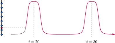
Figure 8. An instance where the red point moves along the trajectory $x_{1}(t)=\sum_{j=0}^{2}\frac{1}{(t-10\cdot j-20)^{4}+1}$. The blue points are stationary, while the red point moves along a trajectory of degree $8$. The red point is the second point to start moving through the blue points (at $t=20$). The trajectory is shown as an arrow along the 1D space, where the gray part has already been traversed.

Lemma 5.1.

Any spanning tree on a set of $n$ points $P$ is an $O(n)$-approximation of the EMST.

Proof A.3.

Let $T$ be an EMST on point set $P$ with total edge length $\operatorname{OPT}$. Additionally let $u,v\in P$, and observe that the path along $T$ from $u$ to $v$ is at least the Euclidean distance between $u$ and $v$, $d(u,v)\leq$. Furthermore, any path along an EMST is at most as long as the total length of an EMST, . If we now take an arbitrary spanning tree $T^{\prime}$ on the same point set $P$, then we know that each edge $(u^{\prime},v^{\prime})$ in this spanning tree has at most length $d(u^{\prime},v^{\prime})\leq$. Since $T^{\prime}$ has $n-1$ edges, its total length is $O(n)\cdot\operatorname{OPT}$.

References

- [1] Pankaj K. Agarwal, Jie Gao, Leonidas J. Guibas, Haim Kaplan, Natan Rubin, and Micha Sharir. Stable Delaunay graphs. Discrete & Computational Geometry, 54(4):905–929, 2015.
- [2] Oswin Aichholzer, Franz Aurenhammer, and Ferran Hurtado. Sequences of spanning trees and a fixed tree theorem. Computational Geometry: Theory and Applications, 21(1-2):3–20, 2002.
- [3] Sunil Arya and David M. Mount. A fast and simple algorithm for computing approximate Euclidean minimum spanning trees. In Proc. 27th Symposium on Discrete Algorithms, pages 1220–1233, 2016.
- [4] Andrea Bacciotti and Lionel Rosier. Liapunov Functions and Stability in Control Theory. Springer, 2 edition, 2006.
- [5] Julien Basch, Leonidas J. Guibas, and John Hershberger. Data structures for mobile data. Journal of Algorithms, 31(1):1–28, 1999.
- [6] Ken Been, Martin Nöllenburg, Sheung-Hung Poon, and Alexander Wolff. Optimizing active ranges for consistent dynamic map labeling. Computational Geometry: Theory and Applications, 43(3):312–328, 2010.
- [7] Olivier Bousquet and André Elisseeff. Stability and generalization. Journal of Machine Learning Research, 2:499–526, 2002.
- [8] Peter Brass, Eowyn Cenek, Cristian A. Duncan, Alon Efrat, Cesim Erten, Dan P. Ismailescu, Stephen G. Kobourov, Anna Lubiw, and Joseph S.B. Mitchell. On simultaneous planar graph embeddings. Computational Geometry: Theory and Applications, 36(2):117–130, 2007.
- [9] Peter Bubenik, Vin de Silva, and Jonathan Scott. Metrics for generalized persistence modules. Foundations of Computational Mathematics, 15(6):1501–1531, 2015.
- [10] Richard L. Burden, J. Douglas Faires, and Annette M. Burden. Numerical Analysis. Cengage, 10 edition, 2015.
- [11] David Cohen-Steiner, Herbert Edelsbrunner, and John Harer. Stability of persistence diagrams. In Proc. 21st Symposium on Computational Geometry, pages 263–271, 2005.
- [12] Mark de Berg, Marcel Roeloffzen, and Bettina Speckmann. Kinetic 2-centers in the black-box model. In Proc. 29th Symposium on Computational Geometry, pages 145–154, 2013.
- [13] Stephane Durocher and David Kirkpatrick. Bounded-velocity approximation of mobile Euclidean 2-centres. International Journal of Computational Geometry & Applications, 18(03):161–183, 2008.
- [14] Jeff Erickson. Dense point sets have sparse Delaunay triangulations or “… but not too nasty”. Discrete & Computational Geometry, 33(1):83–115, 2005.
- [15] Fabrizio Frati, Michael Kaufmann, and Stephen G. Kobourov. Constrained simultaneous and near-simultaneous embeddings. Journal of Graph Algorithms and Applications, 13(3):447–465, 2009.
- [16] Jyh-Jong Fu and Richard C.T. Lee. Voronoi diagrams of moving points in the plane. International Journal of Computational Geometry & Applications, 1(01):23–32, 1991.
- [17] Jie Gao, Leonidas J. Guibas, and An Nguyen. Deformable spanners and applications. Computational Geometry: Theory and Applications, 35(1-2):2–19, 2006.
- [18] Andreas Gemsa, Martin Nöllenburg, and Ignaz Rutter. Sliding labels for dynamic point labeling. In Proc. 23rd Canadian Conference on Computational Geometry, pages 205–210, 2011.
- [19] Andreas Gemsa, Martin Nöllenburg, and Ignaz Rutter. Consistent labeling of rotating maps. Journal of Computational Geometry, 7(1):308–331, 2016.
- [20] Wayne Goddard and Henda C. Swart. Distances between graphs under edge operations. Discrete Mathematics, 161(1-3):121–132, 1996.
- [21] Leonidas J. Guibas. Kinetic data structures. In Dinesh P. Mehta and Sartaj Sahni, editors, Handbook of Data Structures and Applications, pages 23–1–23–18. Chapman and Hall/CRC, 2004.
- [22] Leonidas J. Guibas, Joseph S.B. Mitchell, and Thomas Roos. Voronoi diagrams of moving points in the plane. In Proc. 17th International Workshop on Graph-Theoretic Concepts in Computer Science, LNCS 570, pages 113–125, 1992.
- [23] Nicholas J. Higham. Accuracy and Stability of Numerical Algorithms. SIAM, 2002.
- [24] Naoki Katoh, Takeshi Tokuyama, and Kazuo Iwano. On minimum and maximum spanning trees of linearly moving points. In Proc. 33rd Symposium on Foundations of Computer Science, pages 396–405, 1992.
- [25] Robert M. Kitchin. Cognitive maps: What are they and why study them? Journal of Environmental Psychology, 14(1):1–19, 1994.
- [26] Wladimir Markoff. Über Polynome, die in einem gegebenen Intervalle möglichst wenig von Null abweichen. Mathematische Annalen, 77(2):213–258, 1916.
- [27] Clyde Monma and Subhash Suri. Transitions in geometric minimum spanning trees. Discrete & Computational Geometry, 8(3):265–293, 1992.
- [28] Martin Nöllenburg, Valentin Polishchuk, and Mikko Sysikaski. Dynamic one-sided boundary labeling. In Proc. 18th Conference on Advances in Geographic Information Systems, pages 310–319, 2010.
- [29] Zahed Rahmati, Mohammad Ali Abam, Valerie King, Sue Whitesides, and Alireza Zarei. A simple, faster method for kinetic proximity problems. Computational Geometry: Theory and Applications, 48(4):342–359, 2015.
- [30] Zahed Rahmati and Alireza Zarei. Kinetic Euclidean minimum spanning tree in the plane. Journal of Discrete Algorithms, 16:2–11, 2012.
- [31] Theodore J. Rivlin. The Chebyshev Polynomials, volume 40 of Pure and Applied Mathematics. John Wiley & Sons, 1974.
- [32] Natan Rubin. On topological changes in the Delaunay triangulation of moving points. Discrete & Computational Geometry, 49(4):710–746, 2013.
- [33] Natan Rubin. On kinetic Delaunay triangulations: A near-quadratic bound for unit speed motions. Journal of the ACM, 62(3):25, 2015.
- [34] Micha Sharir and Pankaj K. Agarwal. Davenport-Schinzel sequences and their geometric applications. Cambridge University Press, 1995.
- [35] Daniel A. Spielman and Shang-Hua Teng. Smoothed analysis of algorithms: Why the simplex algorithm usually takes polynomial time. Journal of the ACM, 51(3):385–463, 2004.