Iterative Hybrid Precoder and Combiner Design for mmWave MIMO-OFDM Systems

Abstract

This paper investigates the problem of hybrid precoder and combiner design for multiple-input multiple-output (MIMO) orthogonal frequency division multiplexing (OFDM) systems operating in millimeter-wave (mmWave) bands. We propose a novel iterative scheme to design the codebook-based analog precoder and combiner in forward and reverse channels. During each iteration, we apply compressive sensing (CS) technology to efficiently estimate the equivalent MIMO-OFDM mmWave channel. Then, the analog precoder or combiner is obtained based on the orthogonal matching pursuit (OMP) algorithm to alleviate the interference between different data streams as well as maximize the spectral efficiency. The digital precoder and combiner are finally obtained based on the effective baseband channel to further enhance the spectral efficiency. Simulation results demonstrate the proposed iterative hybrid precoder and combiner algorithm has significant performance advantages.

I Introduction

Millimeter wave (mmWave) communications can provide high data rates by leveraging the large unexploited bandwidths ranged from 30GHz to 300GHz, which makes mmWave communication a promising candidate to solve the spectrum congestion problem in the future wireless communication networks [1]-[3]. However, compared with the conventional frequency bands, the propagation loss in the mmWave band is much more severe due to rain attenuation and low penetration. Thanks to the small wavelength of mmWave signals which enables a large array to be packed into a small physical dimension, mmWave communications with massive MIMO systems can provide the significant beamforming gains to overcome severe path loss of mmWave channel as well as enable the transmission of multiple data streams [4].

In the conventional MIMO systems, full-digital precoders and combiners accomplished in digital-domain can adjust both magnitude and phase of the transmit and receive signals. However, these full-digital precoders and combiners require a large number of expensive and energy-intensive radio frequency (RF) chains, analog-to-digital converters (ADCs), and digital-to-analog converters (DACs) which make full-digital precoding and combining schemes impractical in mmWave communication systems [5]. Recently, hybrid architectures have been considered as an emerging technique to solve this issue. The hybrid beamformer can achieve high spectral efficiency and maintain low cost and power assumption compared with the traditional MIMO systems [6]. The hybrid precoding/combining architectures can apply high-dimensional RF precoder with large number of analog phase shifters to compensate the large path loss at mmWave bands. Moreover, a small number of RF chains for low-dimensional digital precoder can provide necessary flexibility to perform spatial multiplexing. The hybrid precoder design problem is usually formulated to solve various matrix factorization problems with constant modulus constraints of the analog precoder, which is imposed by the phase shifters. Particularly, according to the special characteristic of mmWave channel, a codebook-based hybrid precoder design technique has been widely used, where the columns of the analog precoder are selected from pre-specified vectors, such as array response vectors of the channel and discrete Fourier transform (DFT) beamformers.

Most prior works have been devoted to investigating hybrid precoding and combing algorithms in narrowband channels [7]-[9]. In [7],[8], the spatial structure of mmWave channels is exploited to formulate transmit precoding and receive combining problems as an OMP algorithm. In [9], authors propose an iterative algorithm which updates the phases of the phase shifters of the RF precoder and combiner. Extensions to wideband mmWave hybrid precoding systems have been investigated in [10]-[12]. [10] demonstrates the feasibility for millimeter-wave mobile broadband (MMB) to achieve gigabit-per-second data rates at a distance up to 1 km in an urban mobile environment. In [11], a multi-beam transmission diversity scheme for single stream transmission in MIMO-OFDM system is proposed. In [12], the authors consider a limited feedback hybrid precoding system to design precoders and combiners.

In this paper, we consider a wideband mmWave MIMO-OFDM system with unknown channel state information (CSI). We propose a novel iterative hybrid precoder and combiner design in both forward and reverse channel. A CS-based channel estimation is firstly utilized to estimate the effective channel. Then, based on the effective channel, the analog precoder or combiner is obtained using OMP algorithm. Finally, the digital precoder and combiner are obtained to further suppress the interference and maximize the spectral efficiency. Simulation results show that our proposed algorithm can achieve significant performance improvement.

The following notation is used throughout this paper. $(\cdot)^{T}$, $(\cdot)^{H}$, and $(\cdot)^{*}$ are the transpose, conjugate transpose, and conjugate of a matrix, respectively. $\mathbb{E}\{\cdot\}$ denotes statistical expectation. $\mathbb{C}^{M\times N}$ is the set of $M\times N$ matrices with complex entries. $\mathbf{I}_{N}$ represents an $N\times N$ identity matrix. $|\cdot|$ , $\|\cdot\|$, and $\|\cdot\|_{F}$ are the scalar magnitude, vector norm, and Frobenius norm, respectively. $[\cdot]_{r,:}$ and $[\cdot]_{:,c}$ are the $r$th row and $c$th column of a matrix.

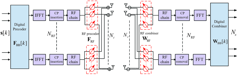
Figure 1: The hybrid precoding and combining architecture in a MIMO-OFDM system.

II System and Problem Formulation

In this section, we present the system and channel models for mmWave MIMO-OFDM communications with hybrid precoder and combiner architecture.

II-A System Model

We consider a MIMO-OFDM system with $N$ subcarriers as shown in Fig. 1. A transmitter with $N_{t}$ transmit antennas and $N_{\mathrm{RF}}$ RF chains transmits $N_{s}$ data streams to a receiver which has $N_{r}$ receive antennas and $N_{\mathrm{RF}}$ RF chains. We assume the number of RF chains is subject to the constraints $N_{\mathrm{RF}}\leq N_{t}$ and $N_{\mathrm{RF}}\leq N_{r}$. The number of data streams is constrained as $N_{s}=N_{\mathrm{RF}}$.

At the transmitter, let $\mathbf{s}[k]$, $k=1,\ldots,N$, be the $N_{s}\times 1$ transmitted vector at the $k$th subcarrier, $\mathbb{E}\{\mathbf{s}[k]\mathbf{s}^{H}[k]\}=\frac{1}{N_{s}}\mathbf{I}_{N_{s}}$. The data stream is firstly precoded by the $N_{\mathrm{RF}}\times N_{s}$ digital precoding matrix $\mathbf{F}_{\mathrm{BB}}[k]$, and then transformed to the time-domain by inverse fast Fourier transform (IFFT) operation. After cyclic prefix (CP) insertion, the transmitted signal is precodered by the $N_{t}\times N_{\mathrm{RF}}$ analogy precoder $\mathbf{F}_{\mathrm{RF}}$. Note that the digital precoding matrix $\mathbf{F}_{\mathrm{BB}}[k]$ can be different for each subcarrier, the analog precoding matrix $\mathbf{F}_{\mathrm{RF}}\in\mathcal{F}$ is the same for all subcarriers due to the special hybrid precoding constructure, where $\mathcal{F}$ is the codebook for the analog precoders which are implemented by analog components like phase shifters, i.e. a set of $N_{t}\times 1$ vectors with quantized phases and constant magnitude entries. The transmit signal at the $k$th subcarrier can be expressed as

$$\mathbf{x}[k]=\sqrt{P}\mathbf{F}_{\mathrm{RF}}\mathbf{F}_{\mathrm{BB}}[k]\mathbf{s}[k],k=1,\ldots,N,$$ (1)

where $P$ represents the average transmit power. The main difference between the OFDM-based hybrid precoding and conventional fully-digital precoding is that $\mathbf{F}_{\mathrm{RF}}$ is applied in the time-domain and the same for all subcarriers, while the baseband precoder $\mathbf{F}_{\mathrm{BB}}[k]$ is performed on each subcarrier in the frequency-domain.

At the receiver, the received signal is combined by the $N_{r}\times N_{\mathrm{RF}}$ RF combining matrix $\mathbf{W}_{\mathrm{RF}}$. The constraint of RF combiner $\mathbf{W}_{\mathrm{RF}}$ is similar to the RF precoder $\mathbf{F}_{\mathrm{RF}}$, i.e. $\mathbf{W}_{\mathrm{RF}}\in\mathcal{W}$, where $\mathcal{W}$ is the set of feasible RF combiners. After RF combining, the CP is removed, and then the time-domain signal is transformed to frequency-domain by the FFT operation. Finally, the $N_{\mathrm{RF}}\times N_{s}$ digital combing matrix $\mathbf{W}_{\mathrm{BB}}[k]$ is employed to process the signal at the $k$th subcarrier. Let $\mathbf{H}[k]\in\mathbb{C}^{N_{r}\times N_{t}}$ denote the channel at the $k$th subcarrier, the received signal after combing at the $k$th subcarrier can be expressed as

$$\begin{split}\mathbf{y}[k]=&\sqrt{P}\mathbf{W}^{H}_{\mathrm{BB}}[k]\mathbf{W}^{H}_{\mathrm{RF}}\mathbf{H}[k]\mathbf{F}_{\mathrm{RF}}\mathbf{F}_{\mathrm{BB}}[k]\mathbf{s}[k]\\ &+\mathbf{W}^{H}_{\mathrm{BB}}[k]\mathbf{W}^{H}_{\mathrm{RF}}\mathbf{n}[k],k=1,\ldots,N,\end{split}$$ (2)

where $\mathbf{n}[k]\sim\mathcal{CN}(0,\sigma_{n}^{2}\mathbf{I})$ is the Gaussian noise vector at the $k$th subcarrier.

II-B Channel Model

We consider a geometric channel model for wideband mmWave channel. For the ease of description, we will use linear antenna array in the channel model. In the $N$-subcarrier OFDM system, the delay-domain channel with $L$ number of paths can be expressed as

$$\mathbf{H}[d]=\sum_{l=1}^{L}\alpha_{l}f(dT_{s}-\tau_{l})\mathbf{a}_{r}(\varphi_{l})\mathbf{a}_{t}^{H}(\phi_{l}),$$ (3)

where $\alpha_{l}$ is the complex path gain of the $l$th channel path, $f(\tau)$ denotes the raised cosine pulse filter at $\tau$, $T_{s}$ is sampling period, $\tau_{l}\in\mathbb{R}$ is the delay of the $l$th path. $\varphi_{l}$ and $\phi_{l}$ are the angles of arrival (AoA) and departure (AoD), respectively. $\mathbf{a}_{r}(\varphi_{l})$ and $\mathbf{a}_{t}(\phi_{l})$ denote the antenna array response of the transmitter and receiver, respectively,

$$\mathbf{a}_{r}=[1,e^{j\pi\mathrm{sin}(\varphi_{l})},\ldots,e^{j\pi(N_{r}-1)\mathrm{sin}(\varphi_{l})}]^{T},$$ (4)

$$\mathbf{a}_{t}=[1,e^{j\pi\mathrm{sin}(\phi_{l})},\ldots,e^{j\pi(N_{t}-1)\mathrm{sin}(\phi_{l})}]^{T}.$$ (5)

After $N$-point FFT of the delay-domain channel $\mathbf{H}[d]$, we can obtain the frequency-domain channel at the $k$th subcarrier

$$\begin{split}\mathbf{H}[k]=&\sum_{d=0}^{N-1}\mathbf{H}[d]e^{-j\frac{2\pi k}{N}d}\\ =&\sum_{d=0}^{N-1}\sum_{l=1}^{L}\alpha_{l}f(dT_{s}-\tau_{l})\mathbf{a}_{r}(\varphi_{l})\mathbf{a}_{t}^{H}(\phi_{l})e^{-j\frac{2\pi k}{N}d},\end{split}$$ (6)

where $k=0,1,\ldots,N-1,$ denotes the $k$th subcarrier in the OFDM systems.

II-C Problem Formulation

In this paper, we consider the problem of hybrid precoder and combiner design in mmWave MIMO-OFDM systems. We first present the CS-based channel estimation to obtain the effective channel information. Then, with the aid of the CS-based channel estimation, we propose an iterative hybrid precoder and combiner design scheme aiming at maximizing the spectral efficiency which can be expressed as

$$\begin{split}&\mathcal{I}=\frac{1}{N}\sum_{k=1}^{N}\mathrm{log}_{2}\Bigg{(}\bigg{|}\mathbf{I}_{N_{s}}+\frac{P}{N_{s}}\mathbf{R}_{n}^{-1}\mathbf{W}_{\mathrm{{BB}}}^{H}[k]\mathbf{W}^{H}_{\mathrm{{RF}}}\mathbf{H}[k]\mathbf{F}_{\mathrm{{RF}}}\\ &\times\mathbf{F}_{\mathrm{{BB}}}[k]\mathbf{F}_{\mathrm{{BB}}}^{H}[k]\mathbf{F}_{\mathrm{RF}}^{H}\mathbf{H}^{H}[k]\mathbf{W}_{\mathrm{{RF}}}\mathbf{W}_{\mathrm{{BB}}}[k]\bigg{|}\Bigg{)},k=1,\ldots,N.\end{split}$$ (7)

where $\mathbf{R}_{n}\triangleq\sigma_{n}^{2}\mathbf{W}_{\mathrm{{BB}}}^{H}[k]\mathbf{W}^{H}_{\mathrm{{RF}}}\mathbf{W}_{\mathrm{{RF}}}\mathbf{W}_{\mathrm{{BB}}}[k]$.

The optimization problem of (7) is obviously a non-convex problem. Note that the forward channel (transmitter-to-receiver) and the reverse channel (receiver-to-transmitter) are identical in a reciprocal time division duplex (TDD) system. Motivated by this fact, we propose a forward-reverse iterative CS-based hybrid beamformer design algorithm. At each iteration, the transmitter and receiver conditionally determine their optimal beam vectors based on the estimated forward or reverse effective channel information obtained by CS technique. The detailed algorithm is presented in the next section.

III Hybrid Precoder and Combiner Design

III-A Analog Combiner Design with CS-based Forward Channel Estimation

The transmitter firstly transmits some training symbols in order to let the receiver estimate the forward channel. We assume different RF chains are independent with each other and the training signals are transmitted one RF chain by another. The received signal at the $k$th subcarrier for the $i$th RF chain is

$$\mathbf{Y}_{r}^{i}[k]=\mathbf{H}_{r}[k]\mathbf{f}_{\mathrm{RF}_{i}}\mathbf{s},i=1,\ldots,N_{\mathrm{RF}},$$ (8)

where $\mathbf{Y}_{r}^{i}[k]\in\mathbb{C}^{N_{r}\times 1}$ represents the received signal for the $i$th RF chain, $\mathbf{s}=[1,1,\dots,1]^{T}$ represents the training signal for all RF chains. The subscript $``r"$ represents the receiver. In the initial iteration, an random beam vector $\mathbf{f}_{\mathrm{RF}_{i}}$ is adopted in each RF chains since we do not know the exact position of the receiver. With the analog precoder vector $\mathbf{f}_{\mathrm{RF}_{i}}$, the frequency-domain channel vector in the first RF chain can be expressed as

$$\begin{split}\mathbf{h}_{r}^{1}[k]=&\mathbf{H}_{r}[k]\mathbf{f}_{\mathrm{RF}_{1}},\\ =&\sum_{d=0}^{N-1}\sum_{l=1}^{L}\alpha_{l}f(dT_{s}-\tau_{l})e^{-j\frac{2\pi k}{N}d}\mathbf{a}_{r}(\varphi_{l})\mathbf{a}_{t}^{H}(\phi_{l})\mathbf{f}_{\mathrm{RF}_{1}},\\ =&\sum_{d=0}^{N-1}\sum_{l=1}^{L}\underbrace{\alpha_{l}\beta_{1}f(dT_{s}-\tau_{l})e^{-j\frac{2\pi k}{N}d}}_{\gamma_{d,l,k}}\mathbf{a}_{r}(\varphi_{l}),k=1,\ldots,N,\end{split}$$ (9)

where $\beta_{i}\triangleq\mathbf{a}_{t}^{H}(\phi_{l})\mathbf{f}_{\mathrm{RF}_{i}}$, $i=1,\ldots,N_{\mathrm{RF}}$.

We define a dictionary $\mathbf{\Psi}_{r}$ shown in (10) at the top of the next page, where $\theta\in[-90^{\circ},90^{\circ}]$ is the angle resolution, $\mathbf{\Psi}_{r}$ has $L_{r}=180/\theta$ columns. The dictionary $\mathbf{\Psi}_{r}$ can cover the whole angle range since $\theta\in[-90^{\circ},90^{\circ}]$ and produce all possible values of $\mathrm{sin}(\theta)$.

$$\mathbf{\Psi}_{r}=\left[\begin{array}[]{c c c c c c c}1&\ldots&1&1&1&\ldots&1\\ e^{j\pi sin(-90^{\circ}+\theta)}&\ldots&e^{j\pi sin(-\theta)}&1&e^{j\pi sin(\theta)}&\ldots&e^{j\pi sin(-90^{\circ})}\\ e^{j2\pi sin(-90^{\circ}+\theta)}&\ldots&e^{j2\pi sin(-\theta)}&1&e^{j2\pi sin(\theta)}&\ldots&e^{j2\pi sin(-90^{\circ})}\\ \vdots&\ldots&\vdots&\vdots&\vdots&\ldots&\vdots\\ e^{j(N_{r}-1)\pi sin(-90^{\circ}+\theta)}&\ldots&e^{j(N_{r}-1)\pi sin(-\theta)}&1&e^{j(N_{r}-1)\pi sin(\theta)}&\ldots&e^{j(N_{r}-1)\pi sin(-90^{\circ})}\end{array}\right].\vspace*{-0.0 cm}$$ (10)

Then, we can represent the effective channel $\mathbf{h}_{r}^{1}[k]$ as

$$\mathbf{h}_{r}^{1}[k]=\mathbf{\Psi}_{r}\mathbf{x}_{r}^{1}[k],k=1,2,\ldots,N.$$ (11)

If the $i$th column of $\mathbf{\Psi}_{r}$ is equal to $\mathbf{a}_{r}(\varphi_{l})$, then the $i$th entry of $\mathbf{x}_{r}^{1}[k]$ is set to $\gamma_{d,l,k}$. This means that, the expansion vector $\mathbf{x}_{r}^{1}[k]$ of $\mathbf{h}_{r}^{1}[k]$ is sparse, which enables us utilize CS to estimate the effective channel.

After the training for the first RF chain, the other training procedures are similar as above. Let $\widetilde{\mathbf{H}}_{r}[k]$ be the effective channel matrix, $\mathbf{X}_{r}[k]\in\mathbb{C}^{L_{r}\times N_{\mathrm{RF}}}$ be the sparse matrix, and each column of $\mathbf{X}_{r}[k]$ is a sparse vector.

$$\begin{split}&\widetilde{\mathbf{H}}_{r}[k]=[\mathbf{h}_{r}^{1}[k],\mathbf{h}_{r}^{2}[k],\ldots,\mathbf{h}_{r}^{\mathrm{RF}}[k]],k=1,\ldots,N,\\ &\mathbf{X}_{r}[k]=[\mathbf{x}_{r}^{1}[k],\mathbf{x}_{r}^{2}[k],\ldots,\mathbf{x}_{r}^{\mathrm{RF}}[k]],k=1,\ldots,N.\end{split}$$ (12)

We can represent the effective channel matrix $\widetilde{\mathbf{H}}_{r}[k]$ as

$$\widetilde{\mathbf{H}}_{r}[k]=\mathbf{\Psi}_{r}\mathbf{X}_{r}[k],k=1,2,\ldots,N.$$ (13)

Then, $M_{r}$ training transmissions are needed to obtain the measurement signal at the $k$th subcarrier, which can be expressed as

$$\begin{split}\mathbf{R}_{r}[k]=&\mathbf{\Phi}_{r}(\mathbf{Y}_{r}[k]+\mathbf{N}_{r}[k])\\ =&\mathbf{\Phi}_{r}(\mathbf{\Psi}_{r}\mathbf{X}_{r}[k]+\mathbf{N}_{r}[k])\\ =&\mathbf{V}_{r}\mathbf{X}_{r}[k]+\mathbf{\Psi}_{r}\mathbf{N}_{r}[k],k=1,\ldots,N,\end{split}$$ (14)

where $\mathbf{R}_{r}[k]\in\mathbb{C}^{M_{r}\times N_{\mathrm{RF}}}$ is the receive signal matrix, $M_{r}$ is the length of training signal, $\mathbf{\Phi}_{r}\in\mathbb{C}^{M_{r}\times N_{r}}$ is the measurement matrix which is randomly chosen from the set $\{\pm 1,\pm j\}$, $\mathbf{N}_{r}[k]\in\mathbb{C}^{N_{r}\times N_{\mathrm{RF}}}$ is the AWGN matrix at the $k$th subcarrier, $\mathbf{V}_{r}\triangleq\mathbf{\Phi}_{r}\mathbf{\Psi}_{r}$. During the $m$th training transmission, $m=1,\ldots,M_{r}$, the transmitter use $\mathbf{f}_{\mathrm{RF}_{i}}$ as the transmit beam vector, while the receiver uses $\mathbf{\Phi}_{r}(m,:)^{H}$ as the beam vector. To estimate the effective channel $\widetilde{\mathbf{H}}_{r}[k]$, we can use orthogonal matching pursuit (OMP) to estimate $\mathbf{X}_{r}[k]$ and then the effective channel $\widetilde{\mathbf{H}}_{r}[k]$ can be constructed by (13).

With the estimated effective channel $\widetilde{\mathbf{H}}_{r}[k]$, we propose to firstly design the analog combiner which can enhance the channel gain of each data stream channel as well as suppress the interference from each other. Since each subcarrier has its own optimal precoder/combiner, it is difficult to choose the best beam vector to achieve the original goal. Therefore, we turn to seek a suboptimal solution. In particular, by considering each transmit/receiver RF chain pair one by one, we successively select analog precoder and combiner to maximize the corresponding channel gain.

We first calculate the optimal MMSE combiner to maximize the corresponding channel gain as well as mitigating the subcarrier interference. The MMSE combiner for the $k$th subcarrier can be written as

$$\mathbf{\Gamma}_{r}[k]=(\widetilde{\mathbf{H}}_{r}[k]\widetilde{\mathbf{H}}_{r}^{H}[k]+\sigma_{n}^{2}\mathbf{I}_{Nr})^{-1}\widetilde{\mathbf{H}}_{r}[k],$$ (15)

where $\mathbf{\Gamma}_{r}[k]\in\mathbb{C}^{N_{r}\times N_{\mathrm{RF}}},k=1,2,\ldots,N$. We normalize the MMSE combiner $\mathbf{\Gamma}_{r}[k]$ by

$$\big{[}\mathbf{\Gamma}_{r}[k]\big{]}_{:,i}=\frac{\big{[}\mathbf{\Gamma}_{r}[k]\big{]}_{:,i}}{\left\|\big{[}\mathbf{\Gamma}_{r}[k]\big{]}_{:,i}\right\|},i=1,\ldots,N_{\mathrm{RF}}.$$ (16)

For the first data stream channel (i.e. $i=1$), we find the suboptimal analog combiner $\mathbf{w}^{\star}_{\mathrm{{RF_{1}}}}$ by searching all candidate vectors in codebook $\mathcal{W}$ to obtain the largest beamforming gain for all subcarriers:

$$\mathbf{w}_{\mathrm{{RF}_{1}}}^{\star}=\mathrm{arg}\max_{\mathbf{w}_{\mathrm{{RF}}}\in\mathcal{W}}\sum_{k=1}^{N}\big{|}\mathbf{w}^{H}_{\mathrm{{RF}}}\big{[}\mathbf{\Gamma}_{r}[k]\big{]}_{:,1}\big{|}.$$ (17)

Assign $\mathbf{w}_{\mathrm{{RF}_{1}}}^{\star}$ to the combiner matrices

$$\big{[}\mathbf{W}_{\mathrm{{RF}}}^{\star}\big{]}_{:,1}=\mathbf{w}_{\mathrm{{RF}_{1}}}^{\star}.$$ (18)

For the rest $N_{\mathrm{RF}}-1$ data streams, we attempt to successively select combiners to actively avoid the interference of the data streams whose precoders and combiners have been determined. To achieve this goal, the component of previous determined combiners should be removed from other data streams’ channels in such a way that the similar analog combiners would not be selected for the other RF chains. Particularly, let $\mathbf{q}_{1}\triangleq\mathbf{w}_{\mathrm{{RF}_{1}}}^{\star}$ be the components of the determined analog combinder for the first data stream. Before finding the second (i.e. $i=2$) analog combiner, the MMSE combiner will be updated by

$$\big{[}\mathbf{\Gamma}_{r}[k]\big{]}_{:,2}=(\mathbf{I}_{N_{r}}-\mathbf{q}_{1}\mathbf{q}_{1}^{H})\big{[}\mathbf{\Gamma}_{r}[k]\big{]}_{:,2},$$ (19)

and then execute searching precessing as

$$\mathbf{w}_{\mathrm{{RF}_{2}}}^{\star}=\mathrm{arg}\max_{\mathbf{w}_{\mathrm{{RF}}}\in\mathcal{W}}\sum_{k=1}^{N}\big{|}\mathbf{w}^{H}_{\mathrm{{RF}}}\big{[}\mathbf{\Gamma}_{r}[k]\big{]}_{:,2}\big{|}.$$ (20)

The analog combiners for the rest RF chains can be successively selected using the above procedure. Note that when $i>1$, the orthogonal component $\mathbf{q}_{i}$ of the selected combiner $\mathbf{w}_{\mathrm{{RF}_{i}}}^{\star}$ can be obtained by a Gram-Schmidt based procedure:

$$\mathbf{q}_{i}=\mathbf{w}_{\mathrm{RF}_{i}}^{\star}-\sum_{j=1}^{i-1}\mathbf{q}_{j}^{H}\mathbf{w}_{\mathrm{RF}_{i}}^{\star}\mathbf{q}_{j},$$ (21)

$$\mathbf{q}_{i}=\mathbf{q}_{i}/\|\mathbf{q}_{i}\|,i=2,\ldots,N_{\mathrm{RF}}.$$ (22)

This iterative analog combiner design algorithm is summarized in Algorithm 1.

Algorithm 1: Iterative Analog Combiner Design

Input:    $\mathcal{W}$, $\mathbf{\Gamma}_{r}[k]$, $\widetilde{\mathbf{H}}_{r}[k]$, $k=1,\ldots,N$.

Output:    $\mathbf{W}_{\mathrm{{RF}}}$.

for $i=1:N_{\mathrm{{RF}}}$

$\mathbf{w}_{\mathrm{RF}}^{\star}(:,i)=\textrm{arg}\underset{\begin{subarray}{c}\mathbf{W}_{\mathrm{{RF}}}\in\mathcal{W}\end{subarray}}{\textrm{max}}\sum_{k=1}^{N}\big{|}\mathbf{w}^{H}_{\mathrm{{RF}}}\big{[}\mathbf{\Gamma}_{r}[k]\big{]}_{:,i}\big{|}$;

$\big{[}\mathbf{W}_{\mathrm{{RF}}}^{\star}\big{]}_{:,i}=\mathbf{w}_{\mathrm{RF}_{i}}^{\star};$

if $i=1$,

$\mathbf{q}_{i}=\mathbf{w}_{\mathrm{RF}_{i}}^{\star}$;

else

$\mathbf{q}_{i}=\mathbf{w}_{\mathrm{RF}_{i}}^{\star}-\sum_{j=1}^{i-1}\mathbf{q}_{j}^{H}\mathbf{w}_{\mathrm{RF}_{i}}^{\star}\mathbf{q}_{j}=\mathbf{q}_{i}/\parallel\mathbf{q}_{i}\parallel$;

end if

$\big{[}\mathbf{\Gamma}_{r}[k]\big{]}_{:,i}=(\mathbf{I}_{N_{r}}-\mathbf{q}_{i}\mathbf{q}_{i}^{H})\big{[}\mathbf{\Gamma}_{r}[k]\big{]}_{:,i}$;

end for

III-B Analog Precoder Design with Reverse Channel Estimation

With the obtained analog combiner $\mathbf{W}^{\star}_{\mathrm{RF}}$ at the receiver, the channel estimation and hybrid precoder design in reverse channel are similar as those in forward channel. The achievable spectral efficiency of the reverse channel system is

$$\begin{split}&\mathcal{I}_{t}=\frac{1}{N}\sum_{k=1}^{N}\mathrm{log}_{2}\Big{(}\big{|}\mathbf{I}_{N_{s}}+\frac{P}{N_{s}}\mathbf{R}_{t}^{-1}\mathbf{F}_{\mathrm{BB}}^{H}[k]\mathbf{F}^{H}_{\mathrm{RF}}\mathbf{H}_{r}^{H}[k]\mathbf{W}_{\mathrm{RF}}\\ &\times\mathbf{W}_{\mathrm{{BB}}}[k]\mathbf{W}_{\mathrm{{BB}}}^{H}[k]\mathbf{W}_{\mathrm{{RF}}}^{H}\mathbf{H}_{r}[k]\mathbf{F}_{\mathrm{RF}}\mathbf{F}_{\mathrm{BB}}[k]\big{|}\Big{)},k=1,\ldots,N,\end{split}$$ (23)

where the subscript “$t$” represents the transmitter, $\mathbf{R}_{t}\triangleq\sigma_{t}^{2}\mathbf{F}_{\mathrm{{BB}}}^{H}[k]\mathbf{F}^{H}_{\mathrm{{RF}}}\mathbf{F}_{\mathrm{{BB}}}[k]\mathbf{F}_{\mathrm{{RF}}}$ is the noise convariance of the reverse channel.

Since the analog combiner $\mathbf{W}_{\mathrm{RF}}$ is available, the receiver also transmits $M_{t}$ training symbols to estimate the effective reverse channel. The received signal at the transmitter is

$$\begin{split}\mathbf{Y}_{t}^{i}[k]=\mathbf{H}_{r}^{H}[k]\mathbf{w}_{\mathrm{RF}_{i}}\mathbf{s},i=1,\ldots,N_{\mathrm{RF}},\end{split}$$ (24)

where $\mathbf{Y}_{t}^{i}[k]\in\mathbb{C}^{N_{t}\times 1}$ denotes the received signal for the $i$th RF chain. Similar to (12), let $\widetilde{\mathbf{H}}_{t}[k]$ represent the effective reverse channel and we have

$$\widetilde{\mathbf{H}}_{t}[k]=\mathbf{\Psi}_{t}\mathbf{X}_{t}[k],k=1,\ldots,N,$$ (25)

where $\mathbf{\Psi}_{t}$ is the dictionary of size $N_{t}\times L_{t}$ with $L_{t}=L_{r}$, and it is the same as $\mathbf{\Psi}_{r}$ except that the term $N_{r}$ in (10) is replaced with $N_{t}$. The signal after measuring can be expressed as follows

$$\begin{split}\mathbf{R}_{t}[k]=&\mathbf{\Phi}_{t}(\mathbf{Y}_{t}[k]+\mathbf{N}_{t}[k])\\ =&\mathbf{\Phi}_{t}(\mathbf{\Psi}_{t}\mathbf{X}_{t}[k]+\mathbf{N}_{t}[k])\\ =&\mathbf{V}_{t}\mathbf{X}_{t}[k]+\mathbf{\Psi}_{t}\mathbf{N}_{t}[k],k=1,\ldots,N,\end{split}$$ (26)

where $\mathbf{R}_{t}[k]$ is the receive signal matrix of size ${M_{t}\times N_{\mathrm{RF}}}$, $\mathbf{\Phi}_{t}\in\mathbb{C}^{M_{t}\times N_{t}}$ is the measurement matrix, and the other notations are similar to those in (14). We can obtain the effective channel $\widetilde{\mathbf{H}}_{t}[k]$ based on CS technique in a similar way to obtain $\widetilde{\mathbf{H}}_{r}[k]$.

The MMSE of reverse channel can be written as

$$\mathbf{\Gamma}_{t}[k]=(\widetilde{\mathbf{H}}_{t}[k]\widetilde{\mathbf{H}}_{t}^{H}[k]+\mathbf{I}_{Nt})^{-1}\widetilde{\mathbf{H}}_{t}[k],$$ (27)

where $\mathbf{\Gamma}_{t}[k]$ is MMSE matrix of size $N_{t}\times N_{\mathrm{RF}}$. Similar to the determination of the analog combiner $\mathbf{W}^{\star}_{\mathrm{{RF}}}$, the analog precoder $\mathbf{F}_{\mathrm{{RF}}}$ is selected by searching through the columns of codebook $\mathcal{F}$:

$$\mathbf{f}_{\mathrm{RF}_{i}}^{\star}=\mathrm{arg}\max_{\mathbf{f}_{\mathrm{{RF}}}\in\mathcal{F}}\sum_{k=1}^{N}\big{|}\mathbf{f}^{H}_{\mathrm{{RF}}}\big{[}\mathbf{\Gamma}_{t}[k]\big{]}_{:,i}\big{|},i=1,\dots,N_{\mathrm{RF}}.$$ (28)

Assign $\mathbf{f}_{\mathrm{RF}_{i}}^{\star}$ to the precoder matrices

$$\big{[}\mathbf{F}_{\mathrm{{RF}}}^{\star}\big{]}_{:,i}=\mathbf{f}_{\mathrm{RF}_{i}}^{\star},i=1,\dots,N_{\mathrm{RF}}.$$ (29)

The following procedure is similar as Algorithm 1 proposed above. After obtaining the analog precoder $\mathbf{F}_{\mathrm{{RF}}}^{\star}$, the first iteration is completed. We then use the obtained analog precoder above as a start point and iteratively design the analog precoder and combiner in forward and reverse transmissions. During the next iteration, a similar process repeats. After $M_{r}$ training transmissions from the transmitter, the receiver will estimate the effective channel $\widetilde{\mathbf{H}}_{r}[k]$ and then renew the combiner $\mathbf{W}_{\mathrm{{RF}}}^{\star}$ by maximizing the spectral efficiency (similar to (17)). Next, based on the $M_{t}$ training transmission from the receiver, the transmitter estimates the effective channel $\widetilde{\mathbf{H}}_{t}[k]$ and then updates the precoder by searching through the codebook (similar to (28)). The iteration procedure continues until the convergence is found or the iteration times exceeds a pre-specified number.

III-C Digital Precoder and Combiner Design

After all analog beamformer pairs for RF chains have been determined, the baseband digital precoder and combiner are computed to further mitigate the interference and maximize the spectral efficiency. We can obtain the effective baseband channel as

$$\mathbf{H}_{e}[k]=\mathbf{W}_{\mathrm{{RF}}}^{H}\widetilde{\mathbf{H}}_{r}[k],k=1,\dots,N.$$ (30)

We perform singular value decomposition (SVD)

$$\mathbf{H}_{e}[k]=\mathbf{U}_{k}\mathbf{\Sigma}_{k}\mathbf{V}_{k}^{H},k=1,\dots,N,$$ (31)

where $\mathbf{U}_{k}$ is an $N_{r}\times N_{r}$ unitary matrix, $\mathbf{\Sigma}_{k}$ is an $N_{r}\times N_{t}$ diagonal matrix of singular values, and $\mathbf{V}_{k}$ is an $N_{t}\times N_{t}$ unitary matrix. Then, the digital precoder and combiner can be obtained by

$$\begin{split}\mathbf{F}_{\mathrm{{BB}}}^{\star}[k]=\mathbf{V}_{k}(:,1:N_{\mathrm{RF}}),\\ \mathbf{W}_{\mathrm{{BB}}}^{\star}[k]=\mathbf{U}_{k}(:,1:N_{\mathrm{RF}}).\end{split}$$ (32)

Finally, the digital precoder and combiner can be normalized by

$$\begin{split}\mathbf{F}_{\mathrm{{BB}}}[k]&=\frac{\sqrt{N_{s}}\mathbf{F}_{\mathrm{BB}}[k]}{\|\mathbf{F}_{\mathrm{{RF}}}\mathbf{F}_{\mathrm{BB}}[k]\|_{F}},k=1,\ldots,N,\\ \mathbf{W}_{\mathrm{{BB}}}[k]&=\frac{\sqrt{N_{s}}\mathbf{W}_{\mathrm{BB}}[k]}{\|\mathbf{W}_{\mathrm{{RF}}}\mathbf{W}_{\mathrm{BB}}[k]\|_{F}},k=1,\ldots,N.\end{split}$$ (33)

IV Simulation Results

In this section, we illustrate the simulation results of the proposed iterative hybrid precoder and combiner design. We consider a mmWave MIMO-OFDM system where both the transmitter and receiver are equipped with 32-antenna ULAs and the antenna spacing is $d=\frac{\lambda}{2}$. The number of channel paths is set as $L=6$. The elevation of the AoA/AoD is assumed to be uniformly distributed in $[-\frac{\pi}{2},\frac{\pi}{2}]$. The number of RF chains at transmitter and receiver are $N_{\mathrm{RF}}=4$, so is the number of data streams $N_{s}=4$. We employ two codebooks consist of a series of array response vectors with 64 uniformly quantized angle resolutions. For the comparison purpose, we also evaluate the approximate Gram-Schmidt based hybrid precoding algorithm [13], which greedily selects the RF beamforming vectors using Gram-Schmidt orthogonalization. Moreover, the greedy hybrid precoding/combining algorithm is proposed with the assumption of perfect CSI.

Fig. 2 shows the spectral efficiency versus signal-to-noise-ratio (SNR) over $10^{5}$ channel realizations in mmWave MIMO-OFDM system. The number of subcarriers is $N=32$ and the CP length is $N_{\mathrm{cp}}=8$. We can observe that the spectral efficiency of our proposed iterative hybrid precoder and combiner design is higher than the Gram-Schmidt based greedy hybrid precoding and combining algorithm. A mmWave MIMO-OFDM system with $N=128$ subcarriers and $N_{\mathrm{cp}}=32$ is shown in Fig. 3 which has similar conclusions. The spectral efficiency of the two algorithms will be improved with the number of subcarriers increasing. It can be observed from these two figures that our proposed algorithm has better performance compared with the existing algorithm.

Fig. 4 shows the spectral efficiency versus SNR using different number of RF chains in mmWave MIMO-OFDM systems. Similar conclusions can be drawn that our proposed iterative hybrid precoding/combining algorithm can achieve significant performance improvement. In addition, our proposed hybrid precoding/combining algorithm with $N_{\mathrm{RF}}=8$ has better performance than the case of $N_{\mathrm{RF}}=4$. We can observe that the larger number of RF chains, the better performance can be achieved in mmWave systems.

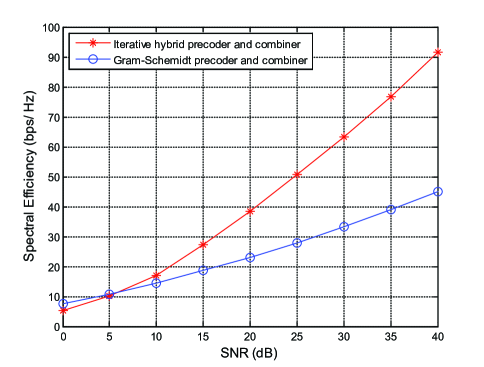
Figure 2: Spectral efficiency versus SNR ($N=32,N_{t}=N_{r}=32,N_{\mathrm{RF}}=4$).

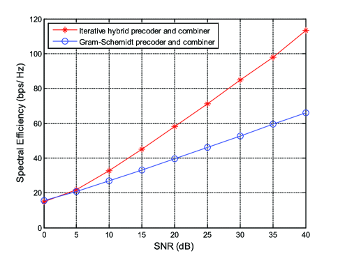
Figure 3: Spectral efficiency versus SNR ($N=128,N_{t}=N_{r}=32,N_{\mathrm{RF}}=4$).

Figure 4: Spectral efficiency versus SNR ($N=32,N_{t}=N_{r}=32$).

V Conclusions

This paper considered the problem of iterative hybrid precoder and combiner design in mmWave MIMO-OFDM systems. We proposed an iterative scheme to successively select the analog precoder and combiner in forward and reverse channels. A CS-based channel estimation is firstly utilized to estimate the effective channel. Then, based on the effective channel, the analog precoder or combiner can be obtained by OMP algorithm. Finally, the digital precoder and combiner are computed to further suppress the interference and maximize the spectral efficiency. Simulation results demonstrate that our proposed scheme can achieve significant performance improvement.

References

- [1] R. W. Heath Jr, N. Gonz lez-Prelcic, S. Rangan, W. Roh, and A. M. Sayeed, “ An overview of signal processing techniques for millimeter wave MIMO systems,” IEEE J. Sel. Topics Signal Process., vol. 10, no. 3, pp. 436-453, April 2016.
- [2] S. Rangan, T. Rappaport, and E. Erkip, “ Millimeter-wave cellular wireless networks: Potentials and challenges,” Proc. of the IEEE, vol. 102, no. 3, pp. 366-385, Mar. 2014.
- [3] J. Andrews, S. Buzzi, W. Choi, S. Hanly, A. Lozano, A. Soong, and J. Zhang, “ What will 5G be?” IEEE J. Sel. Areas commun., vol. 32, no. 6, pp. 1065-1082, June 2014.
- [4] X. Yu, J. Shen, J. Zhang, and K. B. Letaief, “Alternating minimization algorithms for hybrid precoding in millimeter wave MIMO systems,” IEEE J. Select. Topics in Signal Process., vol. 10, no. 3, pp. 485-500, April 2016.
- [5] X. Gao, L. Dai, S. Han, Chih-Lin I, and R. W. Heath Jr., “Energy efficient hybrid analog and digital precoding for mmWave MIMO systems with large antenna arrays,” IEEE J. Sel. Areas Commun., vol. 34, no. 4, pp. 998-1009, April 2016.
- [6] A. Alkhateeb, J. Mo, N. Gonzalez-Prelcic, and R. W. Heath Jr., “MIMO precoding and combining solutions for millimeter-wave systems,” IEEE Commun. Mag., vol. 52, no. 12, pp. 122-131, Dec. 2014.
- [7] O. E. Ayach, S. Rajagopal, S. Abu-Surra, Z. Pi, and R. W. Heath Jr., “Spatially sparse precoding in millimeter wave MIMO systems,” IEEE Trans. Wireless Commun., vol. 13, no. 3, pp. 1499-1513, Mar. 2014.
- [8] A. Alkhateeb, O. E. Ayach, G. Leus, and R. W. Heath Jr., “Hybrid precoding for millimeter wave cellular systems with partial channel knowledge,” in Proc. of Inform. Theory Applicat. Workshop (ITA), San Diego, USA, Feb. 2013, pp. 1-5.
- [9] C. Chen, “An iterative hybrid transceiver design algorithm for millimeter wave MIMO systems,” IEEE Wireless Commun. Lett., vol. 4, no. 3, pp. 285-288, Jun. 2015.
- [10] Z. Pi and F. Khan, “An introduction to millimeter-wave mobile broadband systems,” IEEE Commun. Mag., vol. 49, no. 6, pp. 101-107, Jun. 2011.
- [11] C. Kim, T. Kim, and J. Seol, “Multi-beam transmission diversity with hybrid beamforming for MIMO-OFDM systems,” in Proc. IEEE Globecom Workshops (GC Wkshps), Atlanta, GA, Dec. 2013, pp. 61-65.
- [12] A. Alkhateeb and R. W. Heath Jr., “Frequency selective hybrid precoding for limited feedback millimeter wave systems,” IEEE Trans. Commun., vol. 64, no. 5, pp. 1801-1818, May 2016.
- [13] A. Alkhateeb and R. W. Heath Jr., “Gram Schmidt based greedy hybrid precoding for frequency selective millimeter wave MIMO systems,” in Proc. IEEE Int. Conf. Acoustics, Speech and Signal Process. (ICASSP), Shanghai, China, March 2016, pp. 3396-3400.