Robust Estimators and Test-Statistics for One-Shot Device Testing Under the Exponential Distribution

Abstract

This paper develops a new family of estimators, the minimum density power divergence estimators (MDPDEs), for the parameters of the one-shot device model as well as a new family of test statistics, Z-type test statistics based on MDPDEs, for testing the corresponding model parameters. The family of MDPDEs contains as a particular case the maximum likelihood estimator (MLE) considered in Balakrishnan and Ling (2012). Through a simulation study, it is shown that some MDPDEs have a better behavior than the MLE in relation to robustness. At the same time, it can be seen that some Z-type tests based on MDPDEs have a better behavior than the classical Z-test statistic also in terms of robustness.

1 Introduction

The reliability of a product, system, weapon, or piece of equipment can be defined as the ability of the device to perform as designed, or, more simply, as the probability that the device does not fail when used. Engineers’s assess reliability by repeatedly testing the device and observing its failure rate. Certain products, called “one-shot” devices, make this approach challenging. One-shot devices can only be used once and after use the device is either destroyed or must be rebuilt. Consequently, one can only know whether the failure time is either before or after the test time. The outcomes from each of the devices are therefore binary, either left-censored (failure) or right-censored (success). Some examples of one-shot devices are nuclear weapons, space shuttles, automobile air bags, fuel injectors, disposable napkins, heat detectors, and fuses. In survival analysis, these data are called “current status data”. For instance, in animal carcinogenicity experiments, one observes whether a tumor occurs at the examination time for each subject.

Due to the advances in manufacturing design and technology, products have now become highly reliable with long lifetimes. This fact would pose a problem in the analysis if only few or no failures are observed. For this reason, accelerated life tests are often used by adjusting a controllable factor such as temperature in order to have more failures in the experiment. On the other hand, accelerated life testing would shorten the experimental time and also help to reduce the experimental cost. In this paper, we shall assume that the failure times of devices follow an exponential distribution. In this context, Balakrishnan and Ling (2012) developed the EM algorithm for finding the maximum likelihood estimators of the model parameters. Fan et al. (2009) studied a Bayesian approach for one-shot device testing along with an accelerating factor, in which the failure times of devices is assumed to follows once again an exponential distribution. Rodrigues et al. (1993) presented two approaches based on the likelihood ratio statistics and the posterior Bayes factor for comparing several exponential accelerated life models. Chimitova and Balakrishnan (2015) made a comparison of several goodness-of-fit tests for one-shot device testing.

In Section 2, we present a description of the one-shot device model as well as the maximum likelihood estimators for the model parameters. Section 3 develops the minimum density power divergence estimator as a natural extension of the maximum likelihood estimator, as well as its asymptotic distribution. In Section 4, $Z$-type test statistics are introduced in order to test some hypotheses about the parameters of the one-shot device model. Some numerical examples are presented in Section 5, with one of them relating to a reliability situation and the other two are real applications to tumorigenicity experiments. In Section 6, an extensive simulation study is presented in order to analyze the robustness of the MDPDEs, as well as the $Z$-type test introduced earlier. Finally, some concluding remarks are made in Section 7.

2 Model formulation and maximum likelihood estimator

Consider a reliability testing experiment in which at each time, $t_{j}$, $j=1,2,...,J$, $K$ devices are placed in total under temperatures $w_{i}$, $i=1,...,I$. Therefore, $IJK$ devices are tested in total at temperatures $w_{i}$, $i=1,...,I$, at times $t_{j},$ $j=1,...,J$. It is worth noting that a successful detonation occurs if the lifetime is beyond the inspection time, whereas the lifetime will be before the inspection time if the detonation is a failure. For each temperature $w_{i}$ and at each inspection time $t_{j}$, the number of failures, $n_{ij}$, is then recorded.

In Balakrishnan and Ling (2012), an example is illustrated, in which $30$ devices were tested at temperatures $w_{i}\in\{35,$ $45,$ $55\}$, each with $10$ units being detonated at times $t_{j}\in\{10,$ $20,$ $30\}$, respectively.  In this example, we have $I=3$, $J=3$ and $K=10$. The number of failures observed is summarized in the $3\times 3$ table given in Table 1. In this one-shot device testing experiment, there were in all $48$ failures out a total of $90$ tested devices.

Table 1: Failures in the-shot device testing experiment of Balakrishnan and Ling (2012).

$t_{1}=10$ $t_{2}=20$ $t_{3}=30$ $w_{1}=35$ $3$ $3$ $7$ $w_{2}=45$ $1$ $5$ $7$ $w_{3}=55$ $6$ $7$ $9$

We shall assume here, in accordance Balakrishnan and Ling  (2012), that the true lifetimes $T_{ijk}$, where $i=1,2,...,I$, $j=1,2,...,J$, $k=1,...,K$, are independent and identically distributed exponential random variables with probability density function

$$f(t|\lambda)=\lambda\exp\left(-\lambda t\right),$$

where $\lambda>0$ is the unknown failure rate. In practice, we consider inspection times $t_{j}$, $j=1,...,J$, rather than $t>0$, and we relate the parameter $\lambda$ to an accelerating factor of temperature $w_{i}>0$ through a log-linear link function as

$$\lambda_{w_{i}}(\boldsymbol{\alpha})=\alpha_{0}\exp\left\{\alpha_{1}w_{i}\right\},$$

where $\alpha_{0}>0$ and $\alpha_{1}\in\mathbb{R}$ are unknown parameters. Therefore, the corresponding distribution function is

$$F(t_{j}|\lambda_{w_{i}}(\boldsymbol{\alpha})) =1-\exp\left\{-\lambda_{w_{i}}(\boldsymbol{\alpha})t_{j}\right\}$$

$$=1-\exp\left\{-\alpha_{0}\exp\left\{\alpha_{1}w_{i}\right\}t_{j}\right\}$$ (1)

and the density function

$$f(t_{j}|\lambda_{w_{i}}(\boldsymbol{\alpha}))=\alpha_{0}\exp\left\{\alpha_{1}w_{i}\right\}\exp\left\{-\alpha_{0}\exp\left\{\alpha_{1}w_{i}\right\}t_{j}\right\}.$$ (2)

The data are completely described on $K$ devices, through the contingency table of failures $\boldsymbol{n}=(n_{11},...,n_{1J},...,\allowbreak n_{I1},...,n_{IJ})^{T}$, collected at the temperatures $\boldsymbol{w}=(w_{1},...,w_{I})^{T}$ and the inspection times $\boldsymbol{t}=(t_{1},...,t_{J})^{T}$.

We shall consider the theoretical probability vector $\boldsymbol{p}(\boldsymbol{\alpha})$ defined by

$$\boldsymbol{p}(\boldsymbol{\alpha})= \left(\tfrac{F(t_{1}|\lambda_{w_{1}}(\boldsymbol{\alpha}))}{IJ},\tfrac{1-F(t_{1}|\lambda_{w_{1}}(\boldsymbol{\alpha}))}{IJ},\right.$$

$$\left....,\tfrac{F(t_{J}|\lambda_{w_{I}}(\boldsymbol{\alpha}))}{IJ},\tfrac{1-F(t_{J}|\lambda_{w_{I}}(\boldsymbol{\alpha}))}{IJ}\right)^{T},$$

as well as the observed probability vector

$$\widehat{\boldsymbol{p}}=\left(\tfrac{n_{11}}{IJK},\tfrac{K-n_{11}}{IJK},...,\tfrac{n_{IJ}}{IJK},\tfrac{K-n_{IJ}}{IJK}\right)^{T},$$

both of dimension $2IJ$. Then the Kullback-Leibler divergence between the probability vectors $\widehat{\boldsymbol{p}}$ and $\boldsymbol{p}(\boldsymbol{\alpha})$ is given by

$$d_{KL}\left(\widehat{\boldsymbol{p}},\boldsymbol{p}(\boldsymbol{\alpha})\right) =\frac{1}{IJ}\sum\limits_{i=1}^{I}\sum\limits_{j=1}^{J}\left(\frac{n_{ij}}{K}\log\frac{n_{ij}}{KF(t_{j}|\lambda_{w_{i}}(\boldsymbol{\alpha}))}\right.$$

$$+\left.\frac{K-n_{ij}}{K}\log\frac{K-n_{ij}}{K\left(1-F(t_{j}|\lambda_{w_{i}}(\boldsymbol{\alpha}))\right)}\right).$$

It is not difficult to establish the following result.

Theorem 1

The likelihood function

$$\mathcal{L}\left(\boldsymbol{\alpha}\left|K,\boldsymbol{n},\boldsymbol{t},\boldsymbol{w}\right.\right)=\prod\limits_{i=1}^{I}\prod\limits_{j=1}^{J}F(t_{j}|\lambda_{w_{i}}(\boldsymbol{\alpha}))^{n_{ij}}$$

$$\left(1-F(t_{j}|\lambda_{w_{i}}(\boldsymbol{\alpha}))\right)^{K-n_{ij}},$$

where $F(t_{j}|\lambda_{w_{i}}(\boldsymbol{\alpha}))$ is given by (1), is related to the Kullback-Leibler divergence between the probability vectors $\widehat{\boldsymbol{p}}$ and $\boldsymbol{p}(\boldsymbol{\alpha})$ through

$$d_{KL}\left(\widehat{\boldsymbol{p}},\boldsymbol{p}(\boldsymbol{\alpha})\right)=\frac{1}{IJK}\left(s-\log\mathcal{L}\left(\boldsymbol{\alpha}\left|K,\boldsymbol{n},\boldsymbol{t},\boldsymbol{w}\right.\right)\right),$$ (3)

with $s$ being a constant not dependent on $\boldsymbol{\alpha}$.

Based on the previous result, we have the following definition for the maximum likelihood estimators of $\alpha_{0}$ and $\alpha_{1}.$

Definition 2

We consider the data given by $K$, $\boldsymbol{n}$, $\boldsymbol{t}$, $\boldsymbol{w}$ for the one-shot device model. Then, the maximum likelihood estimator of $\boldsymbol{\alpha}=(\alpha_{0},\alpha_{1})^{T}$, $\widehat{\boldsymbol{\alpha}}=(\widehat{\alpha}_{0},\widehat{\alpha}_{1})^{T}$, can be defined as

$$\widehat{\boldsymbol{\alpha}}=\arg\min_{\boldsymbol{\alpha}\in\Theta}d_{KL}\left(\widehat{\boldsymbol{p}},\boldsymbol{p}(\boldsymbol{\alpha})\right),$$ (4)

where $\Theta=(\mathbb{R}^{+},\mathbb{R})^{T}$.

3 Minimum density power divergence estimator

Based on expression (4), we can think of defining an estimator minimizing any distance or divergence between the probability vectors $\widehat{\boldsymbol{p}}$ and $\boldsymbol{p}(\boldsymbol{\alpha})$. There are many different divergence measures (or distances) known in the lierature, see, for instance, Pardo (2006) and Basu et al. (2011), and the natural question is if all of them are valid to define estimators with good properties. Initially the answer is yes, but we must think in terms of efficiency as well as robustness of the defined estimators. From an asymptotic point of view, it is well-known that the maximum likelihood estimator is a BAN (Best Asymptotically Normal) estimator, but at the same time we know that the maximum likelihood estimator has a very poor behavior, in general, in relation to robustness. It is well-known that a gain in robustness leads to a loss of efficiency. Therefore, the distances (divergence measures) that we must use are those which result in estimators having good properties in terms of robustness with low loss of efficiency. The density power divergence measure introduced by Basu et al. (1998) has the required properties and has been studied for many different problems until now. For more details, see Ghosh et al. (2016), Basu et al. (2016) and the references therein.

Based on Ghosh and Basu (2013), the MDPDE of $\boldsymbol{\alpha}$ is first introduced, and later in Result 4 it is shown that this estimator can be considered as a natural extension of (4).

Definition 3

Let $y_{ijk}$ , $i=1,2,...,I$, $j=1,2,...,J$, $k=1,...,K$, be a sequence of independent Bernoulli random variables, $y_{ijk}\overset{ind}{\sim}Ber(\pi_{ij}(\boldsymbol{\alpha}))$, such that $\pi_{ij}(\boldsymbol{\alpha})=F\left(t_{j}|\lambda_{w_{i}}(\boldsymbol{\alpha})\right)$ and $n_{ij}={\textstyle\sum\nolimits_{k=1}^{K}}y_{ijk}$. The MDPDE of $\boldsymbol{\alpha}$, with tuning parameter $\beta\geq 0$, is given by

$$\widehat{\boldsymbol{\alpha}}_{\beta}=\arg\min_{\boldsymbol{\alpha}\in\Theta}\frac{1}{IJK}\sum\limits_{i=1}^{I}\sum\limits_{j=1}^{J}\sum\limits_{k=1}^{K}V_{ij}\left(y_{ijk},\beta\right),$$ (5)

where

$$V_{ij}\left(y_{ijk},\beta\right) =\pi_{ij}^{\beta+1}(\boldsymbol{\alpha})+(1-\pi_{ij}(\boldsymbol{\alpha}))^{\beta+1}$$

$$-\frac{1+\beta}{\beta}\left(\pi_{ij}^{y_{ijk}}(\boldsymbol{\alpha})(1-\pi_{ij}(\boldsymbol{\alpha}))^{1-y_{ijk}}\right)^{\beta}.$$

For more details about the interpretation of Definition 3, see formula 2.3 in Ghosh and Basu (2013), in which $\pi_{ij}^{y_{ijk}}(\boldsymbol{\alpha})(1-\pi_{ij}(\boldsymbol{\alpha}))^{1-y_{ijk}}$ plays the role of the density in our context. Notice that the expression to be minimized in (5) can be simplified as

$$\frac{1}{IJK}\sum\limits_{i=1}^{I}\sum\limits_{j=1}^{J}\sum\limits_{k=1}^{K}\left\{\pi_{ij}^{\beta+1}(\boldsymbol{\alpha})+(1-\pi_{ij}(\boldsymbol{\alpha}))^{\beta+1}\right.$$

$$\left.-\frac{1+\beta}{\beta}\left(\pi_{ij}^{y_{ijk}}(\boldsymbol{\alpha})(1-\pi_{ij}(\boldsymbol{\alpha}))^{1-y_{ijk}}\right)^{\beta}\right\}$$

$$=\frac{1}{IJ}\sum\limits_{i=1}^{I}\sum\limits_{j=1}^{J}\left\{\pi_{ij}^{\beta+1}(\boldsymbol{\alpha})+(1-\pi_{ij}(\boldsymbol{\alpha}))^{\beta+1}\right.$$

$$\left.-\frac{1+\beta}{\beta}\frac{n_{ij}}{K}\pi_{ij}^{\beta}(\boldsymbol{\alpha})-\frac{1+\beta}{\beta}\frac{K-n_{ij}}{K}(1-\pi_{ij}(\boldsymbol{\alpha}))^{\beta}\right\}.$$ (6)

The following result provides an alternative expression for $\widehat{\boldsymbol{\alpha}}_{\beta}$, given in Definition 3, which is closer to (4) in its expression, since only a divergence measure between two probabilities is involved. Given two probability vectors $\boldsymbol{p}=\left(p_{1},...,p_{M}\right)^{T}$ and $\boldsymbol{q}=\left(q_{1},...,q_{M}\right)^{T}$, the power density divergence measure between $\boldsymbol{p}$ and $\boldsymbol{q}$, with tuning parameter $\beta>0$, is given by

$$d_{\beta}\left(\boldsymbol{p},\boldsymbol{q}\right)=\sum\limits_{j=1}^{M}\left\{q_{j}^{\beta+1}-(1+\tfrac{1}{\beta})q_{j}^{\beta}p_{j}+\tfrac{1}{\beta}p_{j}^{1+\beta}\right\},$$

and for $\beta=0$,

$$d_{0}\left(\boldsymbol{p},\boldsymbol{q}\right)=\lim_{\beta\rightarrow 0^{+}}d_{\beta}\left(\boldsymbol{p},\boldsymbol{q}\right)=d_{KL}\left(\boldsymbol{p},\boldsymbol{q}\right).$$

Therefore, the density power divergence measure between the probability vectors $\widehat{\boldsymbol{p}}$ and $\boldsymbol{p}(\boldsymbol{\alpha})$, with tuning parameter $\beta>0$, has the expression

$$d_{\beta}\left(\widehat{\boldsymbol{p}},\boldsymbol{p}(\boldsymbol{\alpha})\right) =\frac{1}{(IJ)^{\beta+1}}\sum\limits_{i=1}^{I}\sum\limits_{j=1}^{J}\left\{\pi_{ij}^{1+\beta}(\boldsymbol{\alpha})\right.$$

$$\left.-\tfrac{\beta+1}{\beta}\pi_{ij}^{\beta}(\boldsymbol{\alpha})\frac{n_{ij}}{K}+\tfrac{1}{\beta}\left(\frac{n_{ij}}{K}\right)^{1+\beta}\right.$$

$$\left.+\left(1-\pi_{ij}(\boldsymbol{\alpha})\right)^{1+\beta}-\tfrac{\beta+1}{\beta}\left(1-\pi_{ij}(\boldsymbol{\alpha})\right)^{\beta}\tfrac{K-n_{ij}}{K}\right.$$

$$\left.+\tfrac{1}{\beta}\left(\frac{K-n_{ij}}{K}\right)^{1+\beta}\right\},$$ (7)

and for $\beta=0$

$$d_{\beta=0}\left(\widehat{\boldsymbol{p}},\boldsymbol{p}(\boldsymbol{\alpha})\right)=\lim_{\beta\rightarrow 0^{+}}d_{\beta}\left(\widehat{\boldsymbol{p}},\boldsymbol{p}(\boldsymbol{\alpha})\right)=d_{KL}\left(\widehat{\boldsymbol{p}},\boldsymbol{p}(\boldsymbol{\alpha})\right).$$

Theorem 4

The MDPDE of $\boldsymbol{\alpha}$, with tuning parameter $\beta\geq 0$, given in Definition 3, can be alternatively defined as

$$\widehat{\boldsymbol{\alpha}}_{\beta}=\arg\min_{\boldsymbol{\alpha}\in\Theta}d_{\beta}\left(\widehat{\boldsymbol{p}},\boldsymbol{p}(\boldsymbol{\alpha})\right),$$ (8)

where $d_{\beta}\left(\widehat{\boldsymbol{p}},\boldsymbol{p}(\boldsymbol{\alpha})\right)$ is as in (7).

In the following result, the estimating equations needed to get the MDPDEs are presented.

Theorem 5

The MDPDE of $\boldsymbol{\alpha}$ with tuning parameter $\beta\geq 0$, $\widehat{\boldsymbol{\alpha}}_{\beta}$, can be obtained as the solution of equations (9) and (10).

$$\sum\limits_{i=1}^{I}\sum\limits_{j=1}^{J}\left(K\ F(t_{j}|\lambda_{w_{i}}(\boldsymbol{\alpha}))-n_{ij}\right)f(t_{j}|\lambda_{w_{i}}(\boldsymbol{\alpha}))t_{j}\left[F^{\beta-1}(t_{j}|\lambda_{w_{i}}(\boldsymbol{\alpha}))+\left(1-F(t_{j}|\lambda_{w_{i}}(\boldsymbol{\alpha}))\right)^{\beta-1}\right]=0$$ (9)

$$\sum\limits_{i=1}^{I}\sum\limits_{j=1}^{J}\left(K\ F(t_{j}|\lambda_{w_{i}}(\boldsymbol{\alpha}))-n_{ij}\right)f(t_{j}|\lambda_{w_{i}}(\boldsymbol{\alpha}))t_{j}w_{i}\left[F^{\beta-1}(t_{j}|\lambda_{w_{i}}(\boldsymbol{\alpha}))+\left(1-F(t_{j}|\lambda_{w_{i}}(\boldsymbol{\alpha}))\right)^{\beta-1}\right]=0.$$ (10)

In the following results, the asymptotic distribution of the MDPDE of $\boldsymbol{\alpha}$, $\widehat{\boldsymbol{\alpha}}_{\beta}$, for the one-shot device model is presented.

Theorem 6

The asymptotic distribution of the MDPDE $\widehat{\boldsymbol{\alpha}}_{\beta}$ is given by

$$\sqrt{K}\left(\widehat{\boldsymbol{\alpha}}_{\beta}-\boldsymbol{\alpha}_{0}\right)\overset{\mathcal{L}}{\underset{K\mathcal{\rightarrow}\infty}{\longrightarrow}}\mathcal{N}\left(\boldsymbol{0},\boldsymbol{\bar{J}}_{\beta}^{-1}(\boldsymbol{\alpha}_{0})\boldsymbol{\bar{K}}_{\beta}(\boldsymbol{\alpha}_{0})\boldsymbol{\bar{J}}_{\beta}^{-1}(\boldsymbol{\alpha}_{0})\right),$$

where

$$\boldsymbol{\bar{J}}_{\beta}(\boldsymbol{\alpha}) =\sum\limits_{i=1}^{I}\begin{pmatrix}\frac{1}{\alpha_{0}^{2}}&\frac{w_{i}}{\alpha_{0}}\\ \frac{w_{i}}{\alpha_{0}}&w_{i}^{2}\end{pmatrix}\sum\limits_{j=1}^{J}t_{j}^{2}f^{2}(t_{j}|\lambda_{w_{i}}(\boldsymbol{\alpha}))$$

$$\times\left[F^{\beta-1}(t_{j}|\lambda_{w_{i}}(\boldsymbol{\alpha}))+(1-F(t_{j}|\lambda_{w_{i}}(\boldsymbol{\alpha})))^{\beta-1}\right],$$ (11)

$$\boldsymbol{\bar{K}}_{\beta}(\boldsymbol{\alpha}) =\sum\limits_{i=1}^{I}\begin{pmatrix}\frac{1}{\alpha_{0}^{2}}&\frac{w_{i}}{\alpha_{0}}\\ \frac{w_{i}}{\alpha_{0}}&w_{i}^{2}\end{pmatrix}\sum\limits_{j=1}^{J}t_{j}^{2}f^{2}(t_{j}|\lambda_{w_{i}}(\boldsymbol{\alpha}))$$

$$\times\left\{\left[F^{2\beta-1}(t_{j}|\lambda_{w_{i}}(\boldsymbol{\alpha}))+(1-F(t_{j}|\lambda_{w_{i}}(\boldsymbol{\alpha})))^{2\beta-1}\right]\right.$$

$$\left.-\left[F^{\beta}(t_{j}|\lambda_{w_{i}}(\boldsymbol{\alpha}))-(1-F(t_{j}|\lambda_{w_{i}}(\boldsymbol{\alpha})))^{\beta}\right]^{2}\right\},$$ (12)

and $F(t_{j}|\lambda_{w_{i}}(\boldsymbol{\alpha}))$ and $f(t_{j}|\lambda_{w_{i}}(\boldsymbol{\alpha}))$ are given by (1) and (2), respectively.

Since $\widehat{\boldsymbol{\alpha}}_{\beta=0}$ is the MLE of $\boldsymbol{\alpha}$, obtained by maximizing $\log\mathcal{L}\left(\boldsymbol{\alpha}\left|K,\boldsymbol{n},\boldsymbol{t},\boldsymbol{w}\right.\right)$, or equivalently by minimizing

$$d_{\beta=0}\left(\widehat{\boldsymbol{p}},\boldsymbol{p}(\boldsymbol{\alpha})\right) =\lim_{\beta\rightarrow 0^{-}}d_{\beta}\left(\widehat{\boldsymbol{p}},\boldsymbol{p}(\boldsymbol{\alpha})\right)=d_{KL}\left(\widehat{\boldsymbol{p}},\boldsymbol{p}(\boldsymbol{\alpha})\right)$$

$$=\frac{1}{IJK}\left(s-\log\mathcal{L}\left(\boldsymbol{\alpha}\left|K,\boldsymbol{n},\boldsymbol{t},\boldsymbol{w}\right.\right)\right),$$

the following result relates the asymptotic distribution of $\widehat{\boldsymbol{\alpha}}_{\beta=0}$ given previously in terms of $\boldsymbol{\bar{J}}_{\beta=0}(\boldsymbol{\alpha}_{0})$ and $\boldsymbol{\bar{K}}_{\beta=0}(\boldsymbol{\alpha}_{0})$, with respect to the Fisher information matrix, well-known in the classical asymptotic theory of the MLEs.

Theorem 7

The asymptotic distribution of the MLE of $\boldsymbol{\alpha}$, $\widehat{\boldsymbol{\alpha}}_{\beta=0}$, is

$$\sqrt{K}\left(\widehat{\boldsymbol{\alpha}}_{\beta}-\boldsymbol{\alpha}_{0}\right)\overset{\mathcal{L}}{\underset{K\mathcal{\rightarrow}\infty}{\longrightarrow}}\mathcal{N}\left(\boldsymbol{0},\tfrac{1}{IJ}\boldsymbol{I}_{F}^{-1}\left(\boldsymbol{\alpha}_{0}\right)\right),$$

where

$$\boldsymbol{I}_{F}\left(\boldsymbol{\alpha}\right)=\frac{1}{IJ}\sum\limits_{i=1}^{I}\begin{pmatrix}\frac{1}{\alpha_{0}^{2}}&\frac{w_{i}}{\alpha_{0}}\\ \frac{w_{i}}{\alpha_{0}}&w_{i}^{2}\end{pmatrix}\sum\limits_{j=1}^{J}t_{j}^{2}\frac{f^{2}(t_{j}|\lambda_{w_{i}}(\boldsymbol{\alpha}))}{F(t_{j}|\lambda_{w_{i}}(\boldsymbol{\alpha}))(1-F(t_{j}|\lambda_{w_{i}}(\boldsymbol{\alpha})))}$$

4 Robust Z-type tests

For testing the null hypothesis of a linear combination of $\boldsymbol{\alpha}=(\alpha_{0},\alpha_{1})^{T}$, $H_{0}$: $m_{0}\alpha_{0}+m_{1}\alpha_{1}=d$, or equivalently

$$H_{0}\text{: }\boldsymbol{m}^{T}\boldsymbol{\alpha}=d,$$ (13)

where $\boldsymbol{m}^{T}=(m_{0},m_{1})$, it is important to know the asymptotic distribution of the MDPDE of $\boldsymbol{\alpha}$. In particular, in case we wish to test if the different temperatures do not affect the model of the one-shot devices, $\boldsymbol{m}^{T}=(m_{0},m_{1})=(0,1)$ and $d=0$ must be considered. In the following definition, we present $Z$-type test statistics based on $\widehat{\boldsymbol{\alpha}}_{\beta}$. Since $Z$-type test statistics are a particular case of the Wald-type test, we can say that this type of robust test statistics have been considered previously in Basu et al. (2016) and Ghosh et al. (2016).

Definition 8

Let $\widehat{\boldsymbol{\alpha}}_{\beta}=(\widehat{\alpha}_{0,\beta},\widehat{\alpha}_{1,\beta})^{T}$ be the MDPDE of $\boldsymbol{\alpha}=(\alpha_{0},\alpha_{1})^{T}$. The family of $Z$-type test statistics for testing (13) is given by

$$Z_{K}(\widehat{\boldsymbol{\alpha}}_{\beta})=\sqrt{\frac{K}{\boldsymbol{m}^{T}\boldsymbol{\bar{J}}_{\beta}^{-1}(\widehat{\boldsymbol{\alpha}}_{\beta})\boldsymbol{\bar{K}}_{\beta}(\widehat{\boldsymbol{\alpha}}_{\beta})\boldsymbol{\bar{J}}_{\beta}^{-1}(\widehat{\boldsymbol{\alpha}}_{\beta})\boldsymbol{m}}}(\boldsymbol{m}^{T}\widehat{\boldsymbol{\alpha}}_{\beta}-d).$$ (14)

In the following theorem, the asymptotic distribution of $Z_{K}(\widehat{\boldsymbol{\alpha}}_{\beta})$ is presented.

Theorem 9

The asymptotic distribution of $Z$-type test statistics, $Z_{K}(\widehat{\boldsymbol{\alpha}}_{\beta})$, defined in (14), is standard normal.

Based on the previous result, the null hypothesis given in (13) will be rejected, with significance level $\alpha$, if $\left|Z_{K}(\widehat{\boldsymbol{\alpha}}_{\beta})\right|>z_{\frac{\alpha}{2}}$, where $z_{\frac{\alpha}{2}}$ is a right hand side quantile of order $\frac{\alpha}{2}$ of a normal distribution. Now we are going to present a result in order to provide an approximation for the test statistic defined in (14).

Theorem 10

Let $\boldsymbol{\alpha}^{\ast}\in\Theta$ be the true value of the parameter $\boldsymbol{\alpha}$ so that

$$\widehat{\boldsymbol{\alpha}}_{\beta}\overset{\mathcal{P}}{\underset{K\mathcal{\rightarrow}\infty}{\longrightarrow}}\boldsymbol{\alpha}^{\ast}\in\Theta,$$

and $\boldsymbol{m}^{T}\boldsymbol{\alpha}^{\ast}\neq d$. Then, the approximated power function of the test statistic in (14) at $\boldsymbol{\alpha}^{\ast}$ is given by equation (15), where $\Phi(\cdot)$ is the standard normal distribution function.

$$\pi\left(\boldsymbol{\alpha}^{\ast}\right)\simeq 2\left(1-\Phi\left(z_{\frac{\alpha}{2}}-\sqrt{\frac{K}{\boldsymbol{m}^{T}\boldsymbol{\bar{J}}_{\beta}^{-1}(\boldsymbol{\alpha}^{\ast})\boldsymbol{\bar{K}}_{\beta}(\boldsymbol{\alpha}^{\ast})\boldsymbol{\bar{J}}_{\beta}^{-1}(\boldsymbol{\alpha}^{\ast})\boldsymbol{m}}}(\boldsymbol{m}^{T}\boldsymbol{\alpha}^{\ast}-d)\right)\right)$$ (15)

Remark 11

Based on the previous results, it is possible to establish an explicit expression of the number of devices

$$K=\left[\frac{\boldsymbol{m}^{T}\boldsymbol{\bar{J}}_{\beta}^{-1}(\boldsymbol{\alpha}^{\ast})\boldsymbol{\bar{K}}_{\beta}(\boldsymbol{\alpha}^{\ast})\boldsymbol{\bar{J}}_{\beta}^{-1}(\boldsymbol{\alpha}^{\ast})\boldsymbol{m}}{\boldsymbol{m}^{T}\boldsymbol{\alpha}^{\ast}-d}\left(z_{\frac{\alpha}{2}}-\Phi^{-1}(1-\tfrac{\pi^{\ast}}{2})\right)^{2}\right]+1,$$

placed under temperatures $w_{i}$, $i=1,...,I$, at each time, $t_{j}$, $j=1,2,...,J$, necessary in order to get a fixed power $\pi^{\ast}$ for a specific significance level $\alpha$. Here, $[m]$ denotes $\left[\cdot\right]$ the largest integer less than or equal to $m$.

5 Real data examples

In this section, we present some numerical examples to illustrate the inferential results developed in the precedings sections. The first one is an application to the reliability example considered in Section 2, and the other two are real applications to tumorigenicity experiments considered earlier by other authors.

5.1 Example 1 (Reliability experiment)

Based on the example introduced in Section 2, in this section, the MDPDEs of the parameters of the one-shot device model are considered. As tuning parameter, $\beta\in\{0,$ $0.1,$ $0.2,$ $0.3,$ $0.4,$ $0.5,$ $0.6,$ $0.7,$ $0.8,$ $0.9,$ $1,\;2,\;3,\;4\}$ are taken. In Table 2, apart from the MDPDEs of $\boldsymbol{\alpha}$, the MDPDEs of the reliability function

$$R(t|\lambda_{w_{0}}(\boldsymbol{\alpha}))=1-F(t|\lambda_{w_{0}}(\boldsymbol{\alpha}))=e^{-\lambda_{w_{0}}t}=\exp(-\alpha_{0}e^{\alpha_{1}w_{0}}t)$$

are also presented at mission times (time points in the future at which we are interested in the reliability of the unit) $t\in\{10,20,30\}$, namely $R(10|\lambda_{w_{0}}(\widehat{\boldsymbol{\alpha}}_{\beta}))$, $R(20|\lambda_{w_{0}}(\widehat{\boldsymbol{\alpha}}_{\beta}))$, $R(30|\lambda_{w_{0}}(\widehat{\boldsymbol{\alpha}}_{\beta}))$, as well as the MDPDEs of the mean of the lifetime $T(\lambda_{w_{0}}(\boldsymbol{\alpha}))$, namely,

$$E[T(\lambda_{w_{0}}(\boldsymbol{\alpha}))]=\frac{1}{\lambda_{w_{0}}(\boldsymbol{\alpha})}=\frac{1}{\alpha_{0}e^{\alpha_{1}w_{0}}},$$

under the normal operating temperature $w_{0}=25$.

Table 2 shows that the mean lifetime obtained by the maximum likelihood estimator ($\beta=0$) is greater than that obtained from the alternative MPDPDEs.

Table 2: MDPDEs of the parameters, the reliability function at times $t\in\{10,$ $20,$ $30\}$, and mean of lifetime at normal temperature of $25^{\circ}C$ in one-shot device testing experiment considered by Balakrishnan and Ling (2012).

$\beta$	$\qquad\widehat{\alpha}_{0,\beta}\qquad$	$\qquad\widehat{\alpha}_{1,\beta}\qquad$	$R(10|\lambda_{25}(\widehat{\boldsymbol{\alpha}}_{\beta}))$	$R(20|\lambda_{25}(\widehat{\boldsymbol{\alpha}}_{\beta}))$	$R(30|\lambda_{25}(\widehat{\boldsymbol{\alpha}}_{\beta}))$	$E[T(\lambda_{25}(\widehat{\boldsymbol{\alpha}}_{\beta}))]$
0	0.00487	0.04732	0.85300	0.72761	0.62065	62.89490
0.1	0.00489	0.04722	0.85288	0.72741	0.62039	62.83953
0.2	0.00490	0.04714	0.85277	0.72722	0.62016	62.79031
0.3	0.00491	0.04706	0.85268	0.72706	0.61995	62.74654
0.4	0.00492	0.04700	0.85260	0.72693	0.61978	62.70965
0.5	0.00493	0.04695	0.85253	0.72681	0.61963	62.67944
0.6	0.00494	0.04690	0.85247	0.72671	0.61950	62.65188
0.7	0.00495	0.04687	0.85246	0.72669	0.61947	62.64457
0.8	0.00495	0.04683	0.85236	0.72651	0.61925	62.59732
0.9	0.00496	0.04681	0.85233	0.72646	0.61918	62.58398
1	0.00496	0.04681	0.85239	0.72656	0.61931	62.61131
2	0.00496	0.04679	0.85231	0.72644	0.61915	62.57739
3	0.00494	0.04687	0.85255	0.72684	0.61966	62.68584
4	0.00491	0.04700	0.85292	0.72748	0.62048	62.85869

5.2 Example 2 (ED01 Data)

In 1974, the National Center for Toxicological Research made an experiment on 24000 female mice randomized to a control group or one of seven dose levels of a known carcinogen, called 2-Acetylaminofluorene (2-AAF). Table 1 in Lyndsey and Ryan (1993) shows the results obtained when the highest dose level ($150$ parts per million) was administered. The original study considered four different outcomes: Number of animals dying tumour free (DNT) and with tumour (DWT), and sacrified without tumour (SNT) and with tumour (SWT), summarized over three time intervals at $12$, $18$ and $33$ months. A total of $3355$ mice were involved in the experiment.

Table 3: Number of mice sacrified ($r=0$) and died without tumour ($r=1$) and with tumour ($r=2$) from the ED01 Data

		$r=0$	$r=1$	$r=2$
$IT_{1}=12$	$w=0$	115	22	8
	$w=1$	110	49	16
$IT_{2}=18$	$w=0$	780	42	8
	$w=1$	540	54	26
$IT_{3}=33$	$w=0$	675	200	85
	$w=1$	510	64	51

Balakrishnan et al. (2016a) made an analysis combining SNT and SWT as the sacrificed group ($r=0$); and denoting the cause of DNT as natural death ($r=1$), and the cause of DWT as death due to cancer ($r=2$). This modified data are presented in Table 3, while MDPDEs of the model parameters and the corresponding estimates of mean lifetimes are presented in Table 4. Here $w=0$ refers to control group and $w=1$ is the test group, while $E(T_{1})$ and $E(T_{2})$ are the estimated mean lifetimes for sacrifice or nature death ($r=0,1$) and death due to cancer ($r=2$), respectively.

Table 4: MDPDEs of the parameters and the mean lifetimes of the ED01 experiment

$\beta$	$\widehat{\alpha}_{10}$	$\widehat{\alpha}_{11}$	Ew=0($T_{1}$)	Ew=1($T_{1}$)	$\widehat{\alpha}_{20}$	$\widehat{\alpha}_{21}$	Ew=0($T_{2}$)	Ew=1($T_{2}$)	Ew=0($T$)	Ew=1($T$)
0	0.00617	$-$0.12790	162.233	184.165	0.00236	0.25620	426.425	331.582	117.447	118.299
0.1	0.00702	0.09355	142.352	129.639	0.00250	0.32870	399.794	287.795	104.988	89.392
0.2	0.00698	0.06495	143.302	134.290	0.00250	0.31173	400.433	293.189	105.504	92.072
0.3	0.00703	0.00999	142.253	140.840	0.00249	0.29613	401.393	298.513	105.045	95.708
0.4	0.00690	0.00998	145.019	143.578	0.00249	0.27957	401.602	303.655	106.545	97.484
0.5	0.00677	0.00998	147.662	146.195	0.00249	0.26421	401.839	308.537	107.965	99.175
0.6	0.00666	0.00998	150.085	148.594	0.00283	0.00997	353.925	350.414	105.342	104.296
0.7	0.00682	$-$0.06678	146.635	156.763	0.00249	0.23702	401.985	317.157	107.415	104.876
0.8	0.00680	$-$0.08753	147.020	160.468	0.00279	0.00997	358.642	355.083	104.256	110.508
0.9	0.00679	$-$0.10530	147.321	163.680	0.00278	0.00997	360.357	356.781	104.516	112.141
1	0.00678	$-$0.11980	147.546	166.324	0.00277	0.00995	361.607	358.028	104.739	113.506

From Table 4, some MDPDEs of $\alpha_{11}$ are seen to be negative. As pointed out in Balakrishnan et al. (2016), this can be due to the fact that the true value of it may be quite close to zero. In fact, for the values of the tuning parameter $\beta\in\{0.1,0.2,0.3,0.4,0.5,0.6,0.7\}$, the estimators of $\alpha_{11}$ are very close to zero, meaning that the drug will not increase the hazard rate of the natural death outcome. Furthermore, if we look at the estimates of mean lifetimes, these last estimators show a reduction when the carcinogenic drug is administered, but the other ones, $\beta\in\{0,0.8,0.9,1\}$, do not show this behavior (see Figure 1). Thus, in this case, we observe that the MDPDEs with tuning parameter $\beta\in\{0.1,0.2,0.3,0.4,0.5,0.6,0.7\}$ give a more meaningful result in the context of the laboratory experiment than, in particular, the maximum likelihood estimator ($\beta=0$). The simulation study presented in this paper will prove how, in a general case, MDPDEs with these tuning parameters will also present a better behaviour in terms of robustness.

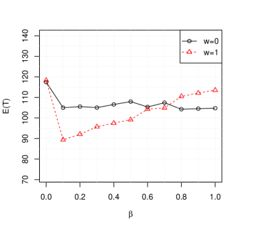
Figure 1: MDPDEs of the mean lifetimes, for different values of the tuning parameter $\beta$, from the ED01 experiment

5.3 Example 3 (Benzidine Dihydrochloride Data)

Table 5: Number of mice sacrified ($r=0$) and died without tumour ($r=1$) and with tumour ($r=2$) from the Benzidine Dihydrochloride Data

		$r=0$	$r=1$	$r=2$
$IT_{1}=9.37$	$w=1$	70	2	0
	$w=2$	22	3	0
$IT_{2}=14.07$	$w=1$	48	1	0
	$w=2$	14	4	17
$IT_{3}=18.7$	$w=1$	35	4	7
	$w=2$	1	1	9

The benzidine dihydrochloride experiment was also conducted at the National Center for Toxicological Research to examine the incidence in mice of liver tumours induced by the drug, and studied by Lyndsey and Ryan (1993) and Balakrishnan et al. (2016b). The inspection times used on the mice were $9.37$, $14.07$ and $18.7$ months. In Table 6, the numbers of mice sacrified ($r=0$), died without tumour ($r=1$) and died with tumour ($r=2$), are shown, for two different doses of drug: $60$ parts per million ($w=1$) and $400$ parts per million ($w=2$). As in the previous example, we consider as “failures” the mice died due to cancer.

Table 6 shows the MDPDEs of the model parameters and the corresponding estimates of mean lifetimes. Although some differences are observed in the results for different values of the tuning parameter, in all the cases, the mean lifetime shows a reduction when the carcinogenic drug is administered.

Table 6: MDPDEs of the parameters and the mean lifetimes of the Benzidine Dihydrochlorid experiment

$\beta$	$\widehat{\alpha}_{10}$	$\widehat{\alpha}_{11}$	Ew=0($T_{1}$)	Ew=1($T_{1}$)	$\widehat{\alpha}_{20}$	$\widehat{\alpha}_{21}$	Ew=1($T_{2}$)	Ew=2($T_{2}$)	Ew=1($T$)	Ew=2($T$)
0	0.00074	1.08665	1342.580	452.912	0.00018	2.49999	5472.201	449.190	1081.274	227.233
0.1	0.00093	0.87121	1072.790	448.905	0.00022	2.45781	4459.410	381.825	867.943	208.460
0.2	0.00097	0.84038	1032.863	445.729	0.00024	2.42125	4110.686	365.071	827.690	202.187
0.3	0.00101	0.81098	994.958	442.182	0.00026	2.39084	3867.836	354.112	790.471	196.024
0.4	0.00104	0.78168	958.766	438.766	0.00029	2.34614	3507.841	335.834	750.183	188.387
0.5	0.00109	0.75071	920.459	434.483	0.00029	2.33901	3449.648	332.624	726.525	188.353
0.6	0.00112	0.72656	893.899	432.261	0.00032	2.29717	3168.017	318.521	695.074	181.946
0.7	0.00115	0.70252	866.492	429.206	0.00032	2.28271	3078.308	314.009	678.390	182.918
0.8	0.00118	0.68232	845.366	427.285	0.00033	2.27346	3011.326	310.030	660.973	180.322
0.9	0.00121	0.66476	826.449	425.122	0.00034	2.25372	2902.649	304.799	645.163	178.887
1	0.00124	0.64796	807.541	422.432	0.00035	2.23942	2823.643	300.774	629.593	176.897

In order to have an idea of the behavior of the different MDPDEs, in relation to the efficiency as well as the robustness, we carry out an extensive simulation study in the next section.

6 Simulation study

In this section, a simulation study is carried out to examine the behavior of the MDPDEs of the parameters of the one-shot device model, studied in Section 3, as well as the $Z$-type tests, based on MDPDEs, detailed in Section 4. We pay special attention to the robustness issue. It is interesting to note, in this context, the following. For each fixed time, $t_{j}$, under a fixed temperature, $w_{i}$, $K$ devices are tested. In this sense, we can identify our data as a $I\times J$ contingency table with $K$ observations in each cell. Hence, under this setting, we must consider “outlying cells” rather than “outlying observations”. A cell which does not follow the one-shot device model will be called an outlying cell or outlier. The strong outliers may lead to reject a model fitting even if the rest of the cells fit the model properly. In other cases, even though the cells seem to fit reasonably well the model, the outlying cells contribute to an increase in the values of the residuals as well as the divergence measure between the data and the fitted values according to the one-shot device model considered. Therefore, it is very important to have robust estimators as well as robust test statistics in order to avoid the undesirable effects of the outliers in the data. The main purpose of this simulation study is to show that inside the family of MDPDEs, developed here, there are estimators with better robust properties than the MLE, and the $Z$-type tests constructed from them are at the same time more robust than the classical $Z$-type test, constructed through the MLEs.

6.1 The MDPDEs

In this section, we carry out a simulation study to compare the behavior of some MDPDEs with respect to the MLEs of the parameters in the one-shot device model under the exponential distribution. In order to evaluate th performance of the proposed MDPDEs, as well as the MLEs, we consider the root of the mean square errors (RMSEs). We have considered a model in which, $I=J=3$, $w\in\{35,$ $45,$ $55\}$, $t\in\{10,$ $20,$ $30\}$ and $K=20$, as in the example in Table 1, and the simulation experiment proposed by Ling (2012). This model has been examined under three choices of $(\alpha_{0},\alpha_{1})=(0.005,0.05)$, $(\alpha_{0},\alpha_{1})=(0.004,0.05)$ and $(\alpha_{0},\alpha_{1})=(0.003,0.05)$ for low-moderate, moderate and moderate-high reliability, respectively.

To evaluate the robustness of the MDPDEs, we have studied the behavior of this model under the consideration of an outlying cell for $(w_{1},t_{1})$ in our contingency table, with $10,000$ replications and estimators corresponding to the tuning parameter $\beta\in\{0,0.1,0.2,0.4,0.6,0.8,1\}$. The reduction of each one of the parameters of the outlying cell, denoted by $\tilde{\alpha}_{0}$ or $\tilde{\alpha}_{1}$ ($\alpha_{0}\geq\tilde{\alpha}_{0}$ or $\alpha_{1}\geq\tilde{\alpha}_{1}$) increases the mean of its lifetime distribution function in (1). The results obtained by decreasing parameter $\alpha_{0}$ are shown in Figure 3(a), while the results obtained by decreasing parameter $\alpha_{1}$ are shown in Figure 3(b). In all the cases, we can see how the MLEs and the MDPDEs with small values of tuning parameter $\beta$ present the smallest RMSEs for weak outliers, i.e., when $\tilde{\alpha}_{0}$ is close to $\alpha_{0}$ ($1-\tilde{\alpha}_{0}/\alpha_{0}$ is close to $0$) or $\tilde{\alpha}_{1}$ is close to $\alpha_{1}$ ($1-\tilde{\alpha}_{1}/\alpha_{1}$ is close to $0$). On the other hand, large values of tuning parameter $\beta$ turn the MDPDEs to present the smallest RMSEs, for medium and strong outliers, i.e., when $\tilde{\alpha}_{0}$ is not close to $\alpha_{0}$ ($1-\tilde{\alpha}_{0}/\alpha_{0}$ is not close to $0$) or $\tilde{\alpha}_{1}$ is not close to $\alpha_{1}$ ($1-\tilde{\alpha}_{1}/\alpha_{1}$ is not close to $0$). Therefore, the MLE of $(\alpha_{0},\alpha_{1})$ is very efficient when there are no outliers, but highly non-robust when there are outliers. On the other hand, the MDPDEs with moderate values of the tuning parameter $\beta$ exhibit a little loss of efficiency without outliers but at the same time a considerable improvement of robustness with outliers. Actually, these values of the tuning parameter $\beta$ are the most appropriate ones for the estimators of the parameters in the one-shot device model according to robustness theory: To improve in a considerable way the robustness of the estimators, a small amount of efficiency needs to be compromised.

6.2 The Z-type tests based on MDPDEs

We will study the performance, with respect to robustness, through simulation of the one-shot device model defined in Section 2 with the same values of $I,J,t,w$ of the example of Balakrishnan and Ling (2012) given in Table 1 and for the same tuning parameter, $\beta$, as in Section 6.1. We are interested in testing the null hypothesis $H_{0}:\alpha_{1}=0.05$ against the alternative $H_{1}:\alpha_{1}\neq 0.05$, through the $Z$-type test statistics based on MDPDEs. Under the null hypothesis, we consider as true parameters $(\alpha_{0},\alpha_{1})=(0.004,0.05)$, while under the alternative we consider as true parameters $(\alpha_{0},\alpha_{1})=(0.004,0.02)$. In Figure 2, we present the empirical significance level (measured as the proportions of test statistics exceeding in absolute value the standard normal quantile critical value) with $10,000$ replications. The empirical power (obtained in a similar manner) is also presented in the right hand side of Figure 2. Notice that in all the cases the observed levels are quite close to the nominal level of $0.05$. The empirical power is similar for the different values of the tuning parameters $\beta$, a bit lower for large values of $\beta$, and closer to one as $K$ or the sample size ($n=IJK$) increases.

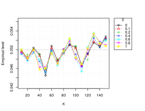
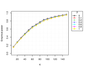
Figure 2: Simulated levels (left) and powers (right) with no outliers in the data.

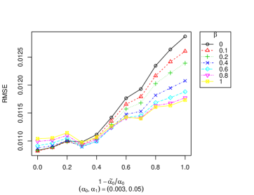
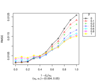
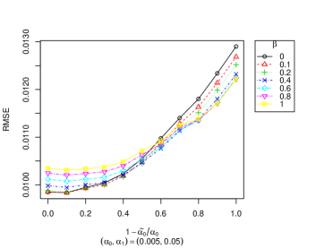
(a) with an $\alpha_{0}$-contaminated outlying cell.

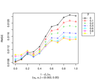
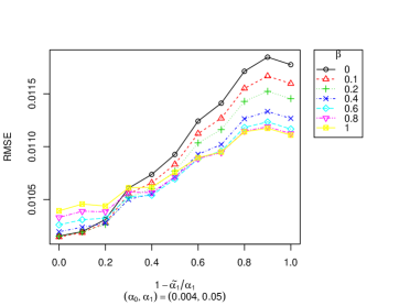
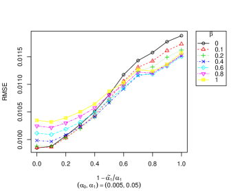
(b) with an $\alpha_{1}$-contaminated outlying cell.

Figure 3: RMSEs of MDPDEs for $\boldsymbol{\alpha}$

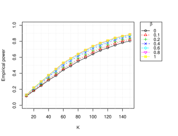
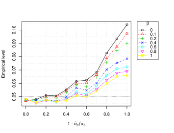
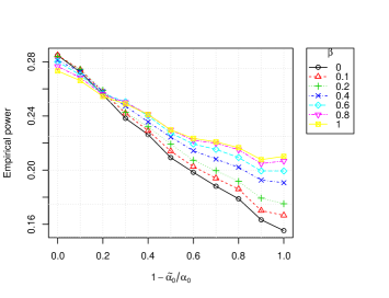
Figure 4: Simulated levels (left) and powers (right) with an $\alpha_{0}$-contaminated outlying cell.

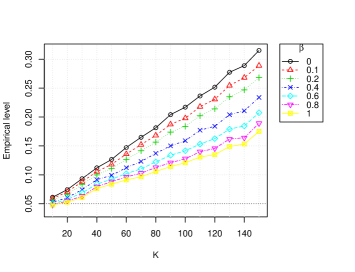
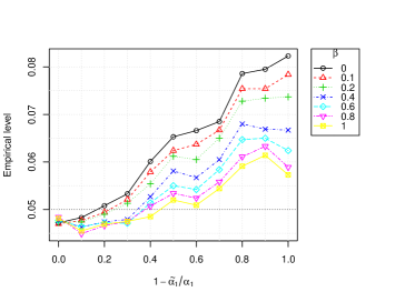
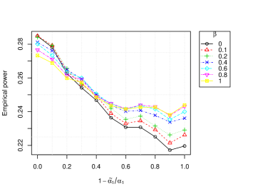
Figure 5: Simulated levels (left) and powers (right) with an $\alpha_{1}$-contaminated outlying cell in the data.

To evaluate the robustness of the level and the power of the $Z$-type tests based on MDPDEs with an outlier placed on the first-row first-column cell, we perform the simulation for the same test and the same true values for the null and alternative hypotheses, in two different scenarios depending on the way the outlying cell is considered. In the first scenario, we keep $\alpha_{1}$ the same and modify the true value of $\alpha_{0}$ to be $\tilde{\alpha}_{0}\leq\alpha_{0}$, and in the second one, we keep $\alpha_{0}$ the same and modify the true value of $\alpha_{1}$ to be $\tilde{\alpha}_{1}\leq\alpha_{1}$. Both cases have been analyzed for different values of $K$ and decreasing $\tilde{\alpha}_{0}$ in the first scenario (increasing $1-\tilde{\alpha}_{0}/\alpha_{0}$) or decreasing $\tilde{\alpha}_{1}$ in the second scenario (increasing $1-\tilde{\alpha}_{1}/\alpha_{1}$).

The results for the first scenario are presented in Figure 4. The empirical level for the one-shot device model with $K$ from $10$ to $150$, true value $(\alpha_{0},\alpha_{1})=(0.004,0.05)$ and $\tilde{\alpha}_{0}=0.001$ for the outlying cell is presented on the left and top panel. Similarly, the empirical power for the one-shot device model with $K$ from $10$ to $150$, true parameter $(\alpha_{0},\alpha_{1})=(0.004,0.02)$ and $\tilde{\alpha}_{0}=0.001$ for the outlying cell is presented on the right top panel. In addition, the empirical level for the one-shot device model with $1-\tilde{\alpha}_{0}/\alpha_{0}$ from $0$ to $1$ for the outlying cell and true value $(\alpha_{0},\alpha_{1})=(0.004,0.05)$ and $K=20$ is presented on the left bottom panel. Similarly, the empirical power for the one-shot device model with $1-\tilde{\alpha}_{0}/\alpha_{0}$ from $0$ to $1$ for the outlying cell and true value and true parameter $(\alpha_{0},\alpha_{1})=(0.004,0.02)$ is presented on the right bottom panel.

Notice that the outlying cell represents 1/9 of the total observations in the last plots. For large values of $K$ (very large sample sizes, since $n=9K$), there is a large inflation in the empirical level and shrinkage of the empirical power, but for the $Z$-type test statistic based on the MDPDEs with large values of the tuning parameter $\beta$, the effect of the outlying cell is weaker in comparison to those of smaller values of $\beta$, included the MLEs ($\beta=0$). If $\tilde{\alpha}_{0}$ is separated from $\alpha_{0}$ ($1-\tilde{\alpha}_{0}/\alpha_{0}$ increases from $0$ to $1$), the empirical level of the $Z$-type test statistics based on the MDPDEs is not stable around the nominal level, being however closer as the tuning parameter $\beta$ becomes larger. If $\tilde{\alpha}_{0}$ is separated from $\alpha_{0}$ ($1-\tilde{\alpha}_{0}/\alpha_{0}$ increases from $0$ to $1$), the empirical power of the $Z$-type test statistics based on the MDPDEs decreases, being however more slowly as the tuning parameter $\beta$ becomes larger.

Figure 5 presents the results for the second scenario, in which $\tilde{\alpha}_{1}=0.01$ for the outlying cell on the left top panel and $\tilde{\alpha}_{1}=-0.01$ for the outlying cell on the right top panel. Even though the outliers are, in the current scenario, slightly more pronunced with respect to the previous scenario, in general terms, we arrive at the same conclusions as in the previous scenario.

The results of the tests statistics presented here show again the poor behavior in robustness of the $Z$-type tests based on the MLE of the parameters of the one-shot device model. Furthermore, the robustness properties of the $Z$-type test statistics based on the MDPDEs with large values of the tuning parameter $\beta$ are often better as they maintain both level and power in a stable manner. Moreover, the comments made at the end of Section 6.1 for the MDPDEs regarding moderate values of the tuning parameter $\beta$ are valid for the $Z$-type test statistics based on the MDPDEs as well.

$$\mathcal{T}_{1,\beta}(\boldsymbol{\alpha})=\sum\limits_{i=1}^{I}\sum\limits_{j=1}^{J}\left\{\left(\frac{F\left(t_{j}|\lambda_{w_{i}}(\boldsymbol{\alpha})\right)}{IJ}\right)^{1+\beta}-(1+\tfrac{1}{\beta})\left(\frac{F\left(t_{j}|\lambda_{w_{i}}(\boldsymbol{\alpha})\right)}{IJ}\right)^{\beta}\frac{n_{ij}}{IJK}+\tfrac{1}{\beta}\left(\frac{n_{ij}}{IJK}\right)^{1+\beta}\right\}$$ (16)

$$\mathcal{T}_{2,\beta}(\boldsymbol{\alpha})=\sum\limits_{i=1}^{I}\sum\limits_{j=1}^{J}\left\{\left(\frac{1-F\left(t_{j}|\lambda_{w_{i}}(\boldsymbol{\alpha})\right)}{IJ}\right)^{1+\beta}-(1+\tfrac{1}{\beta})\left(\frac{1-F\left(t_{j}|\lambda_{w_{i}}(\boldsymbol{\alpha})\right)}{IJ}\right)^{\beta}\frac{K-n_{ij}}{IJK}+\tfrac{1}{\beta}\left(\frac{K-n_{ij}}{IJK}\right)^{1+\beta}\right\}$$ (17)

7 Concluding Remarks

In this paper, we have introduced and studied the minimum density power divergence estimators for one-shot device testing with an accelerating factor of temperature. Based on these estimators, we have also introduced a Wald-type test statistic family. Since the maximum likelihood estimator is a particular estimator in the family of minimum density power divergence estimators developed here, the classical Wald test is also taken into account for comparison. The results obtained in the simulation study suggest that some minimum density power divergence estimators are considerably better for the estimation of the model parameters when outliers are present in the data and at the same time not facing much loss of efficiency when outliers are not present. Similar results are obtained for some Wald-type test statistics in terms of stability with respect to level and power. These proposed estimators also give a more meaningful result in the case of ED01 tumorigenicity experiment data than the maximum likelihood estimators.

Appendix A Proofs of Results

A.1 Proof of Result 1:

We have

$$d_{KL}\left(\widehat{\boldsymbol{p}},\boldsymbol{p}(\boldsymbol{\alpha})\right) =\frac{1}{IJK}\left(s-\sum\limits_{i=1}^{I}\sum\limits_{j=1}^{J}\log\left(F(t_{j}|\lambda_{w_{i}}(\boldsymbol{\alpha}))\right)^{n_{ij}}\right.$$

$$\left.+\sum\limits_{i=1}^{I}\sum\limits_{j=1}^{J}\log\left(\left(1-F(t_{j}|\lambda_{w_{i}}(\boldsymbol{\alpha}))\right)\right)^{K-n_{ij}}\right)$$

$$=\frac{1}{IJK}\left(s-\log\prod\limits_{i=1}^{I}\prod\limits_{j=1}^{J}F(t_{j}|\lambda_{w_{i}}(\boldsymbol{\alpha}))^{n_{ij}}\right.$$

$$\times\left.\left(1-F(t_{j}|\lambda_{w_{i}}(\boldsymbol{\alpha}))\right)^{K-n_{ij}}\right.\Bigg{)}$$

$$=\frac{1}{IJK}\left(s-\log\mathcal{L}\left(\boldsymbol{\alpha}\left|K,\boldsymbol{n},\boldsymbol{t},\boldsymbol{w}\right.\right)\right),$$

with

$$s=\sum\limits_{i=1}^{I}\sum\limits_{j=1}^{J}n_{ij}\log\frac{n_{ij}}{K}+\sum\limits_{i=1}^{I}\sum\limits_{j=1}^{J}(K-n_{ij})\log\frac{K-n_{ij}}{K},$$

as required.

A.2 Proof of Result 4:

The relationship between (6) and $d_{\beta}\left(\widehat{\boldsymbol{p}},\boldsymbol{p}(\boldsymbol{\alpha})\right)$ defined in (7) is given by

$$\frac{1}{IJ}\sum\limits_{i=1}^{I}\sum\limits_{j=1}^{J}\left\{\pi_{ij}^{\beta+1}(\boldsymbol{\alpha})+(1-\pi_{ij}(\boldsymbol{\alpha}))^{\beta+1}\right.$$

$$\left.-\frac{1+\beta}{\beta}\frac{n_{ij}}{K}\pi_{ij}^{\beta}(\boldsymbol{\alpha})-\frac{1+\beta}{\beta}\frac{K-n_{ij}}{K}(1-\pi_{ij}(\boldsymbol{\alpha}))^{\beta}\right\}$$

$$=(IJ)^{\beta+1}d_{\beta}\left(\widehat{\boldsymbol{p}},\boldsymbol{p}(\boldsymbol{\alpha})\right)+c,$$

where $c$ is a constant not dependent on $\boldsymbol{\alpha}$, and so $\widehat{\boldsymbol{\alpha}}_{\beta}$ is the same for both cases. Hence, the result.

A.3 Proof of Result 5:

We have

$$\frac{\partial F(t_{j}|\lambda_{w_{i}}(\boldsymbol{\alpha}))}{\partial\alpha_{0}} =\exp\left\{-\alpha_{0}\exp\left(\alpha_{1}w_{i}\right)t_{j}\right\}\exp\left\{\alpha_{1}w_{i}\right\}t_{j}$$

$$=f(t_{j}|\lambda_{w_{i}}(\boldsymbol{\alpha}))\frac{t_{j}}{\alpha_{0}}$$ (18)

and

$$\frac{\partial F(t_{j}|\lambda_{w_{i}}(\boldsymbol{\alpha}))}{\partial\alpha_{1}}= \exp\left\{-\alpha_{0}\exp\left(\alpha_{1}w_{i}\right)t_{j}\right\}$$

$$\times\exp\left\{\alpha_{1}w_{i}\right\}\alpha_{0}t_{j}w_{i}$$

$$= f(t_{j}|\lambda_{w_{i}}(\boldsymbol{\alpha}))t_{j}w_{i}.$$ (19)

We denote

$$d_{\beta}\left(\widehat{\boldsymbol{p}},\boldsymbol{p}(\boldsymbol{\alpha})\right)=\mathcal{T}_{1,\beta}(\boldsymbol{\alpha})+\mathcal{T}_{2,\beta}(\boldsymbol{\alpha}),$$

where $\mathcal{T}_{1,\beta}(\boldsymbol{\alpha})$ and $\mathcal{T}_{2,\beta}(\boldsymbol{\alpha})$ are given by (16) and (17), respectively, for $\beta>0$.

Based on (18), we have

$$\frac{\partial\mathcal{T}_{1,\beta}(\boldsymbol{\alpha})}{\partial\alpha_{0}}= \frac{\beta+1}{\left(IJ\right)^{\beta+1}}\sum\limits_{i=1}^{I}\sum\limits_{j=1}^{J}\left(F(t_{j}|\lambda_{w_{i}}(\boldsymbol{\alpha}))-\frac{n_{ij}}{K}\right)$$

$$\times f(t_{j}|\lambda_{w_{i}}(\boldsymbol{\alpha}))\frac{t_{j}}{\alpha_{0}}F^{{}^{\beta-1}}(t_{j}|\lambda_{w_{i}}(\boldsymbol{\alpha}))$$

and

$$\frac{\partial\mathcal{T}_{2,\beta}(\boldsymbol{\alpha})}{\partial\alpha_{0}}= \frac{\beta+1}{\left(IJ\right)^{\beta+1}}\sum\limits_{i=1}^{I}\sum\limits_{j=1}^{J}\left(F(t_{j}|\lambda_{w_{i}}(\boldsymbol{\alpha}))-\frac{n_{ij}}{K}\right)$$

$$\times f(t_{j}|\lambda_{w_{i}}(\boldsymbol{\alpha}))\frac{t_{j}}{\alpha_{0}}\left(1-F(t_{j}|\lambda_{w_{i}}(\boldsymbol{\alpha}))\right)^{{}^{\beta-1}}.$$

On the other hand, by (19), we have

$$\frac{\partial\mathcal{T}_{1,\beta}(\boldsymbol{\alpha})}{\partial\alpha_{1}}= \frac{\beta+1}{\left(IJ\right)^{\beta+1}}\sum\limits_{i=1}^{I}\sum\limits_{j=1}^{J}\left(F(t_{j}|\lambda_{w_{i}}(\boldsymbol{\alpha}))-\frac{n_{ij}}{K}\right)$$

$$\times f(t_{j}|\lambda_{w_{i}}(\boldsymbol{\alpha}))t_{j}w_{i}F^{{}^{\beta-1}}(t_{j}|\lambda_{w_{i}}(\boldsymbol{\alpha}))$$

and

$$\frac{\partial\mathcal{T}_{2,\beta}(\boldsymbol{\alpha})}{\partial\alpha_{1}}= \frac{\beta+1}{\left(IJ\right)^{\beta+1}}\sum\limits_{i=1}^{I}\sum\limits_{j=1}^{J}\left(F(t_{j}|\lambda_{w_{i}}(\boldsymbol{\alpha}))-\frac{n_{ij}}{K}\right)$$

$$\times f(t_{j}|\lambda_{w_{i}}(\boldsymbol{\alpha}))t_{j}w_{i}\left(1-F(t_{j}|\lambda_{w_{i}}(\boldsymbol{\alpha}))\right)^{{}^{\beta-1}}.$$

Finally, the system of equations is given by

$$\frac{\left(IJ\right)^{\beta+1}}{\beta+1}\left(\frac{\partial\mathcal{T}_{1,\beta}(\boldsymbol{\alpha})}{\partial\alpha_{0}}+\frac{\partial\mathcal{T}_{2,\beta}(\boldsymbol{\alpha})}{\partial\alpha_{0}}\right) =0,$$

$$\frac{\left(IJ\right)^{\beta+1}}{\beta+1}\left(\frac{\partial\mathcal{T}_{1,\beta}(\boldsymbol{\alpha})}{\partial\alpha_{1}}+\frac{\partial\mathcal{T}_{2,\beta}(\boldsymbol{\alpha})}{\partial\alpha_{1}}\right) =0.$$

If we consider $\beta=0$ in (9) and (10), we get the system needed to solve in order to get the maximum likelihood estimator (MLE). Hence, the previous system of equations is valid not only for tuning parameters $\beta>0$, but also for $\beta=0$.

A.4 Proof of Result 6:

Based on Ghosh and Basu (2013) and also on Definition 3, we have

$$\sqrt{IJK}\left(\widehat{\boldsymbol{\alpha}}_{\beta}-\boldsymbol{\alpha}_{0}\right)\overset{\mathcal{L}}{\underset{IJK\mathcal{\rightarrow}\infty}{\longrightarrow}}\mathcal{N}\left(\boldsymbol{0},\boldsymbol{J}_{\beta}^{-1}(\boldsymbol{\alpha}_{0})\boldsymbol{K}_{\beta}(\boldsymbol{\alpha}_{0})\boldsymbol{J}_{\beta}^{-1}(\boldsymbol{\alpha}_{0})\right),$$

where

$$\boldsymbol{J}_{\beta}(\boldsymbol{\alpha})= \frac{1}{IJK}\sum\limits_{i=1}^{I}\sum\limits_{j=1}^{J}\sum\limits_{k=1}^{K}\boldsymbol{J}_{ij,\beta}(\boldsymbol{\alpha})$$

$$= \frac{1}{IJ}\sum\limits_{i=1}^{I}\sum\limits_{j=1}^{J}\boldsymbol{J}_{ij,\beta}(\boldsymbol{\alpha}),$$

$$\boldsymbol{J}_{ij,\beta}(\boldsymbol{\alpha})= \boldsymbol{u}_{ij}(\boldsymbol{\alpha})\boldsymbol{u}_{ij}^{T}(\boldsymbol{\alpha})F^{\beta+1}(t_{j}|\lambda_{w_{i}}(\boldsymbol{\alpha}))$$

$$+\boldsymbol{v}_{ij}(\boldsymbol{\alpha})\boldsymbol{v}_{ij}^{T}(\boldsymbol{\alpha})(1-F(t_{j}|\lambda_{w_{i}}(\boldsymbol{\alpha})))^{\beta+1}$$

$$= t_{j}^{2}f^{2}(t_{j}|\lambda_{w_{i}}(\boldsymbol{\alpha}))\begin{pmatrix}\frac{1}{\alpha_{0}^{2}}&\frac{w_{i}}{\alpha_{0}}\\ \frac{w_{i}}{\alpha_{0}}&w_{i}^{2}\end{pmatrix}\left[F^{\beta-1}(t_{j}|\lambda_{w_{i}}(\boldsymbol{\alpha}))\right.$$

$$\left.+(1-F(t_{j}|\lambda_{w_{i}}(\boldsymbol{\alpha})))^{\beta-1}\right],$$

$$\boldsymbol{u}_{ij}(\boldsymbol{\alpha})= \frac{\partial\log F(t_{j}|\lambda_{w_{i}}(\boldsymbol{\alpha}))}{\partial\boldsymbol{\alpha}}$$

$$= \frac{1}{F(t_{j}|\lambda_{w_{i}}(\boldsymbol{\alpha}))}\frac{\partial}{\partial\boldsymbol{\alpha}}F(t_{j}|\lambda_{w_{i}}(\boldsymbol{\alpha})),$$

$$\boldsymbol{v}_{ij}(\boldsymbol{\alpha})= \frac{\partial\log\left[1-F(t_{j}|\lambda_{w_{i}}(\boldsymbol{\alpha}))\right]}{\partial\boldsymbol{\alpha}}$$

$$= -\frac{1}{1-F(t_{j}|\lambda_{w_{i}}(\boldsymbol{\alpha}))}\frac{\partial}{\partial\boldsymbol{\alpha}}F(t_{j}|\lambda_{w_{i}}(\boldsymbol{\alpha})),$$

$$\frac{\partial}{\partial\boldsymbol{\alpha}}F(t_{j}|\lambda_{w_{i}}(\boldsymbol{\alpha}))= -\frac{\partial}{\partial\boldsymbol{\alpha}}\exp\left\{-\alpha_{0}\exp\left\{\alpha_{1}w_{i}\right\}t_{j}\right\}$$

$$= \begin{pmatrix}\frac{1}{\alpha_{0}}\\ w_{i}\end{pmatrix}t_{j}f(t_{j}|\lambda_{w_{i}}(\boldsymbol{\alpha})),$$

and

$$\boldsymbol{K}_{\beta}(\boldsymbol{\alpha})= \frac{1}{IJK}\sum\limits_{i=1}^{I}\sum\limits_{j=1}^{J}\sum\limits_{k=1}^{K}\boldsymbol{K}_{ij,\beta}(\boldsymbol{\alpha})$$

$$= \frac{1}{IJ}\sum\limits_{i=1}^{I}\sum\limits_{j=1}^{J}\boldsymbol{K}_{ij,\beta}(\boldsymbol{\alpha}),$$

$$\boldsymbol{K}_{ij,\beta}(\boldsymbol{\alpha})= \boldsymbol{S}_{ij,\boldsymbol{\beta}}(\boldsymbol{\alpha})-\boldsymbol{\xi}_{ij,\beta}(\boldsymbol{\alpha})\boldsymbol{\xi}_{ij,\beta}^{T}(\boldsymbol{\alpha}),$$

$$\boldsymbol{S}_{ij,\boldsymbol{\beta}}(\boldsymbol{\alpha})= \boldsymbol{u}_{ij}(\boldsymbol{\alpha})\boldsymbol{u}_{ij}^{T}(\boldsymbol{\alpha})F^{2\beta+1}(t_{j}|\lambda_{w_{i}}(\boldsymbol{\alpha}))$$

$$+\boldsymbol{v}_{ij}(\boldsymbol{\alpha})\boldsymbol{v}_{ij}^{T}(\boldsymbol{\alpha})(1-F(t_{j}|\lambda_{w_{i}}(\boldsymbol{\alpha})))^{2\beta+1}$$

$$= t_{j}^{2}f^{2}(t_{j}|\lambda_{w_{i}}(\boldsymbol{\alpha})))\begin{pmatrix}\frac{1}{\alpha_{0}^{2}}&\frac{w_{i}}{\alpha_{0}}\\ \frac{w_{i}}{\alpha_{0}}&w_{i}^{2}\end{pmatrix}\left[F^{2\beta-1}(t_{j}|\lambda_{w_{i}}(\boldsymbol{\alpha}))\right.$$

$$\left.+(1-F(t_{j}|\lambda_{w_{i}}(\boldsymbol{\alpha})))^{2\beta-1}\right],$$

$$\boldsymbol{\xi}_{ij,\beta}(\boldsymbol{\alpha})= \boldsymbol{u}_{ij}(\boldsymbol{\alpha})F^{\beta+1}(t_{j}|\lambda_{w_{i}}(\boldsymbol{\alpha}))$$

$$+\boldsymbol{v}_{ij}(\boldsymbol{\alpha})(1-F(t_{j}|\lambda_{w_{i}}(\boldsymbol{\alpha})))^{\beta+1}$$

$$= \begin{pmatrix}\frac{1}{\alpha_{0}}\\ w_{i}\end{pmatrix}t_{j}f(t_{j}|\lambda_{w_{i}}(\boldsymbol{\alpha}))\left[F^{\beta}(t_{j}|\lambda_{w_{i}}(\boldsymbol{\alpha}))\right.$$

$$\left.-(1-F(t_{j}|\lambda_{w_{i}}(\boldsymbol{\alpha})))^{\beta}\right].$$

Since $I$, $J$ are fixed and $IJK\mathcal{\rightarrow}\infty$, it follows that $K\mathcal{\rightarrow}\infty$ and

$$\sqrt{K}\left(\widehat{\boldsymbol{\alpha}}_{\beta}-\boldsymbol{\alpha}_{0}\right)\overset{\mathcal{L}}{\underset{K\mathcal{\rightarrow}\infty}{\longrightarrow}}\mathcal{N}\left(\boldsymbol{0},\boldsymbol{\bar{J}}_{\beta}^{-1}(\boldsymbol{\alpha}_{0})\boldsymbol{\bar{K}}_{\beta}(\boldsymbol{\alpha}_{0})\boldsymbol{\bar{J}}_{\beta}^{-1}(\boldsymbol{\alpha}_{0})\right)$$

where

$$\boldsymbol{\bar{J}}_{\beta}^{-1}(\boldsymbol{\alpha}_{0})\boldsymbol{\bar{K}}_{\beta}(\boldsymbol{\alpha}_{0})\boldsymbol{\bar{J}}_{\beta}^{-1}(\boldsymbol{\alpha}_{0}) =\frac{1}{IJ}\boldsymbol{J}_{\beta}^{-1}(\boldsymbol{\alpha}_{0})\boldsymbol{K}_{\beta}(\boldsymbol{\alpha}_{0})\boldsymbol{J}_{\beta}^{-1}(\boldsymbol{\alpha}_{0}),$$

$$\boldsymbol{\bar{J}}_{\beta}(\boldsymbol{\alpha}_{0}) =(IJ)\boldsymbol{J}_{\beta}(\boldsymbol{\alpha}_{0}),$$

$$\boldsymbol{\bar{K}}_{\beta}(\boldsymbol{\alpha}_{0}) =(IJ)\boldsymbol{K}_{\beta}(\boldsymbol{\alpha}_{0}).$$

A.5 Proof of Result 7:

The Fisher information matrix for $IJK$ observations is

$$\boldsymbol{I}_{IJK,F}\left(\boldsymbol{\alpha}\right)=E\left[-\frac{\partial\boldsymbol{v}^{T}\left(\boldsymbol{\alpha}\left|K,\boldsymbol{n},\boldsymbol{t},\boldsymbol{w}\right.\right)}{\partial\boldsymbol{\alpha}}\right],$$

where

$$\boldsymbol{v}\left(\boldsymbol{\alpha}\left|K,\boldsymbol{n},\boldsymbol{t},\boldsymbol{w}\right.\right)=\frac{\partial\log\mathcal{L}\left(\boldsymbol{\alpha}\left|K,\boldsymbol{n},\boldsymbol{t},\boldsymbol{w}\right.\right)}{\partial\boldsymbol{\alpha}}.$$

From (3),

$$\boldsymbol{I}_{IJK,F}\left(\boldsymbol{\alpha}\right) =IJK\;E\left[\frac{\partial^{2}d_{KL}\left(\widehat{\boldsymbol{p}},\boldsymbol{p}(\boldsymbol{\alpha})\right)}{\partial\boldsymbol{\alpha}\partial\boldsymbol{\alpha}^{T}}\right]$$

$$=IJK\;E\left[\frac{\partial\boldsymbol{u}^{T}\left(\boldsymbol{\alpha}\left|K,\boldsymbol{n},\boldsymbol{t},\boldsymbol{w}\right.\right)}{\partial\boldsymbol{\alpha}}\right],$$

where

$$\boldsymbol{u}\left(\boldsymbol{\alpha}\left|K,\boldsymbol{n},\boldsymbol{t},\boldsymbol{w}\right.\right) =\frac{\partial d_{KL}\left(\widehat{\boldsymbol{p}},\boldsymbol{p}(\boldsymbol{\alpha})\right)}{\partial\boldsymbol{\alpha}}$$

$$=\frac{\partial\mathcal{T}_{1,\beta=0}(\boldsymbol{\alpha})}{\partial\boldsymbol{\alpha}}+\frac{\partial\mathcal{T}_{2,\beta=0}(\boldsymbol{\alpha})}{\partial\boldsymbol{\alpha}}.$$

The Fisher information matrix for a single observation, i.e., the Fisher information matrix for the one-shot device model is

$$\boldsymbol{I}_{F}\left(\boldsymbol{\alpha}\right)=\frac{1}{IJK}\boldsymbol{I}_{IJK,F}\left(\boldsymbol{\alpha}\right)=E\left[\frac{\partial\boldsymbol{u}^{T}\left(\boldsymbol{\alpha}\left|K,\boldsymbol{n},\boldsymbol{t},\boldsymbol{w}\right.\right)}{\partial\boldsymbol{\alpha}}\right].$$

From Result 6, the first and second components of $\boldsymbol{u}\left(\boldsymbol{\alpha}\left|K,\boldsymbol{n},\boldsymbol{t},\boldsymbol{w}\right.\right)$ are

$$u_{1}\left(\boldsymbol{\alpha}\left|K,\boldsymbol{n},\boldsymbol{t},\boldsymbol{w}\right.\right)=\frac{\partial\mathcal{T}_{1,\beta=0}(\boldsymbol{\alpha})}{\partial\alpha_{0}}+\frac{\partial\mathcal{T}_{2,\beta=0}(\boldsymbol{\alpha})}{\partial\alpha_{0}}$$

$$=\frac{1}{IJK}\sum\limits_{i=1}^{I}\sum\limits_{j=1}^{J}\left(K\ F(t_{j}|\lambda_{w_{i}}(\boldsymbol{\alpha}))-n_{ij}\right)$$

$$\ \ \times f(t_{j}|\lambda_{w_{i}}(\boldsymbol{\alpha}))\frac{t_{j}}{\alpha_{0}}\left[F^{-1}(t_{j}|\lambda_{w_{i}}(\boldsymbol{\alpha}))+\left(1-F(t_{j}|\lambda_{w_{i}}(\boldsymbol{\alpha}))\right)^{-1}\right]$$

$$=\frac{1}{IJK}\sum\limits_{i=1}^{I}\sum\limits_{j=1}^{J}\frac{K\ F(t_{j}|\lambda_{w_{i}}(\boldsymbol{\alpha}))-n_{ij}}{F(t_{j}|\lambda_{w_{i}}(\boldsymbol{\alpha}))\left(1-F(t_{j}|\lambda_{w_{i}}(\boldsymbol{\alpha}))\right)}f(t_{j}|\lambda_{w_{i}}(\boldsymbol{\alpha}))\frac{t_{j}}{\alpha_{0}}$$

and

$$u_{2}\left(\boldsymbol{\alpha}\left|K,\boldsymbol{n},\boldsymbol{t},\boldsymbol{w}\right.\right)=\frac{\partial\mathcal{T}_{1,\beta=0}(\boldsymbol{\alpha})}{\partial\alpha_{1}}+\frac{\partial\mathcal{T}_{2,\beta=0}(\boldsymbol{\alpha})}{\partial\alpha_{1}}$$

$$=\frac{1}{IJK}\sum\limits_{i=1}^{I}\sum\limits_{j=1}^{J}\left(K\ F(t_{j}|\lambda_{w_{i}}(\boldsymbol{\alpha}))-n_{ij}\right)$$

$$\ \ \times f(t_{j}|\lambda_{w_{i}}(\boldsymbol{\alpha}))t_{j}w_{i}\left[F^{-1}(t_{j}|\lambda_{w_{i}}(\boldsymbol{\alpha}))+\left(1-F(t_{j}|\lambda_{w_{i}}(\boldsymbol{\alpha}))\right)^{-1}\right]$$

$$=\frac{1}{IJK}\sum\limits_{i=1}^{I}\sum\limits_{j=1}^{J}\frac{K\ F(t_{j}|\lambda_{w_{i}}(\boldsymbol{\alpha}))-n_{ij}}{F(t_{j}|\lambda_{w_{i}}(\boldsymbol{\alpha}))\left(1-F(t_{j}|\lambda_{w_{i}}(\boldsymbol{\alpha}))\right)}f(t_{j}|\lambda_{w_{i}}(\boldsymbol{\alpha}))t_{j}w_{i},$$

respectively. The $(1,1)$th term of $\boldsymbol{I}_{F}\left(\boldsymbol{\alpha}\right)$ is the expectation of

$$\frac{\partial u_{1}\left(\boldsymbol{\alpha}\left|K,\boldsymbol{n},\boldsymbol{t},\boldsymbol{w}\right.\right)}{\partial\alpha_{0}}$$

$$=\frac{1}{IJK}\sum\limits_{i=1}^{I}\sum\limits_{j=1}^{J}\left\{-\frac{t_{j}}{\alpha_{0}^{2}}\frac{K\ F(t_{j}|\lambda_{w_{i}}(\boldsymbol{\alpha}))-n_{ij}}{F(t_{j}|\lambda_{w_{i}}(\boldsymbol{\alpha}))\left(1-F(t_{j}|\lambda_{w_{i}}(\boldsymbol{\alpha}))\right)}f(t_{j}|\lambda_{w_{i}}(\boldsymbol{\alpha}))\right.$$

$$\ \ +\left.\frac{\partial f(t_{j}|\lambda_{w_{i}}(\boldsymbol{\alpha}))}{\partial\alpha_{0}}\frac{t_{j}}{\alpha_{0}}\frac{K\ F(t_{j}|\lambda_{w_{i}}(\boldsymbol{\alpha}))-n_{ij}}{F(t_{j}|\lambda_{w_{i}}(\boldsymbol{\alpha}))\left(1-F(t_{j}|\lambda_{w_{i}}(\boldsymbol{\alpha}))\right)}\right.$$

$$\ \ +\left.\frac{\partial}{\partial\alpha_{0}}\left(\frac{K\ F(t_{j}|\lambda_{w_{i}}(\boldsymbol{\alpha}))-n_{ij}}{F(t_{j}|\lambda_{w_{i}}(\boldsymbol{\alpha}))\left(1-F(t_{j}|\lambda_{w_{i}}(\boldsymbol{\alpha}))\right)}\right)\frac{t_{j}}{\alpha_{0}}f(t_{j}|\lambda_{w_{i}}(\boldsymbol{\alpha}))\right\}.$$

Since the expectation of the first two summands of $\partial u_{1}\left(\boldsymbol{\alpha}\left|K,\boldsymbol{n},\boldsymbol{t},\boldsymbol{w}\right.\right)/\partial\alpha_{0}$ are zero, the interest is on the expectation of $L_{ij}$ which is given in (20).

$$L_{ij} =\frac{\partial}{\partial\alpha_{0}}\left(\frac{K\ F(t_{j}|\lambda_{w_{i}}(\boldsymbol{\alpha}))-n_{ij}}{F(t_{j}|\lambda_{w_{i}}(\boldsymbol{\alpha}))\left(1-F(t_{j}|\lambda_{w_{i}}(\boldsymbol{\alpha}))\right)}\right)\frac{t_{j}}{\alpha_{0}}f(t_{j}|\lambda_{w_{i}}(\boldsymbol{\alpha}))$$

$$=\frac{K\frac{t_{j}}{\alpha_{0}}f(t_{j}|\lambda_{w_{i}}(\boldsymbol{\alpha}))F(t_{j}|\lambda_{w_{i}}(\boldsymbol{\alpha}))\left(1-F(t_{j}|\lambda_{w_{i}}(\boldsymbol{\alpha}))\right)}{F(t_{j}|\lambda_{w_{i}}(\boldsymbol{\alpha}))^{2}\left(1-F(t_{j}|\lambda_{w_{i}}(\boldsymbol{\alpha}))\right)^{2}}\frac{t_{j}}{\alpha_{0}}f(t_{j}|\lambda_{w_{i}}(\boldsymbol{\alpha}))$$

$$-\frac{\frac{\partial}{\partial\alpha_{0}}\left[F(t_{j}|\lambda_{w_{i}}(\boldsymbol{\alpha}))\left(1-F(t_{j}|\lambda_{w_{i}}(\boldsymbol{\alpha}))\right)\right]\left(K\ F(t_{j}|\lambda_{w_{i}}(\boldsymbol{\alpha}))-n_{ij}\right)}{F(t_{j}|\lambda_{w_{i}}(\boldsymbol{\alpha}))^{2}\left(1-F(t_{j}|\lambda_{w_{i}}(\boldsymbol{\alpha}))\right)^{2}}\frac{t_{j}}{\alpha_{0}}f(t_{j}|\lambda_{w_{i}}(\boldsymbol{\alpha})).$$ (20)

The expectation of the second summand of $L_{ij}$ is zero and hence

$$E[L_{ij}]=\frac{K\left(\frac{t_{j}}{\alpha_{0}}\right)^{2}f^{2}(t_{j}|\lambda_{w_{i}}(\boldsymbol{\alpha}))}{F(t_{j}|\lambda_{w_{i}}(\boldsymbol{\alpha}))\left(1-F(t_{j}|\lambda_{w_{i}}(\boldsymbol{\alpha}))\right)}.$$

These finally yield the $(1,1)$th term of $\boldsymbol{I}_{F}\left(\boldsymbol{\alpha}\right)$ as

$$E\left[\frac{\partial u_{1}\left(\boldsymbol{\alpha}\left|K,\boldsymbol{n},\boldsymbol{t},\boldsymbol{w}\right.\right)}{\partial\alpha_{0}}\right]$$

$$=\frac{K}{IJK}\sum\limits_{i=1}^{I}\sum\limits_{j=1}^{J}\frac{\left(\frac{t_{j}}{\alpha_{0}}\right)^{2}f^{2}(t_{j}|\lambda_{w_{i}}(\boldsymbol{\alpha}))}{F(t_{j}|\lambda_{w_{i}}(\boldsymbol{\alpha}))\left(1-F(t_{j}|\lambda_{w_{i}}(\boldsymbol{\alpha}))\right)}$$

$$=\frac{1}{IJ}\sum\limits_{i=1}^{I}\sum\limits_{j=1}^{J}\frac{\left(\frac{t_{j}}{\alpha_{0}}\right)^{2}f^{2}(t_{j}|\lambda_{w_{i}}(\boldsymbol{\alpha}))}{F(t_{j}|\lambda_{w_{i}}(\boldsymbol{\alpha}))\left(1-F(t_{j}|\lambda_{w_{i}}(\boldsymbol{\alpha}))\right)}.$$

The rest of the terms of $\boldsymbol{I}_{F}\left(\boldsymbol{\alpha}\right)$ can be obtained in a similar manner. On the other hand, from Theorem 6, sustituting $\beta=0$ into $\boldsymbol{J}_{\beta}(\boldsymbol{\alpha})=\frac{1}{IJ}\boldsymbol{\bar{J}}_{\beta}(\boldsymbol{\alpha})=$ and $\boldsymbol{K}_{\beta}(\boldsymbol{\alpha})=\frac{1}{IJ}\boldsymbol{\bar{K}}_{\beta}(\boldsymbol{\alpha})$, we simply obtain $\boldsymbol{J}_{\beta=0}(\boldsymbol{\alpha})=\boldsymbol{K}_{\beta=0}(\boldsymbol{\alpha})=\boldsymbol{I}_{F}(\boldsymbol{\alpha})$.

A.6 Proof of Result 9:

Let $\boldsymbol{\alpha}_{0}$ be the true value of parameter $\boldsymbol{\alpha}.$ It is clear that under (13)

$$\boldsymbol{m}^{T}\widehat{\boldsymbol{\alpha}}_{\beta}-d=\boldsymbol{m}^{T}(\widehat{\boldsymbol{\alpha}}_{\beta}-\boldsymbol{\alpha}_{0})$$

and we know

$$\sqrt{K}(\widehat{\boldsymbol{\alpha}}_{\beta}-\boldsymbol{\alpha}_{0})\overset{\mathcal{L}}{\underset{K\mathcal{\rightarrow}\infty}{\longrightarrow}}\mathcal{N}(\boldsymbol{0},\boldsymbol{\bar{J}}_{\beta}^{-1}(\boldsymbol{\alpha}_{0})\boldsymbol{\bar{K}}_{\beta}(\boldsymbol{\alpha}_{0})\boldsymbol{\bar{J}}_{\beta}^{-1}(\boldsymbol{\alpha}_{0})),$$

from which it follows that

$$\sqrt{K}(\boldsymbol{m}^{T}\widehat{\boldsymbol{\alpha}}_{\beta}-d)\overset{\mathcal{L}}{\underset{K\mathcal{\rightarrow}\infty}{\longrightarrow}}\mathcal{N}(0,\boldsymbol{m}^{T}\boldsymbol{\bar{J}}_{\beta}^{-1}(\boldsymbol{\alpha}_{0})\boldsymbol{\bar{K}}_{\beta}(\boldsymbol{\alpha}_{0})\boldsymbol{\bar{J}}_{\beta}^{-1}(\boldsymbol{\alpha}_{0})\boldsymbol{m}).$$

Dividing the left hand side by

$$\sqrt{\boldsymbol{m}^{T}\boldsymbol{\bar{J}}_{\beta}^{-1}(\widehat{\boldsymbol{\alpha}}_{\beta})\boldsymbol{\bar{K}}_{\beta}(\widehat{\boldsymbol{\alpha}}_{\beta})\boldsymbol{\bar{J}}_{\beta}^{-1}(\widehat{\boldsymbol{\alpha}}_{\beta})\boldsymbol{m}},$$

since $\boldsymbol{m}^{T}\boldsymbol{\bar{J}}_{\beta}^{-1}(\widehat{\boldsymbol{\alpha}}_{\beta})\boldsymbol{\bar{K}}_{\beta}(\widehat{\boldsymbol{\alpha}}_{\beta})\boldsymbol{\bar{J}}_{\beta}^{-1}(\widehat{\boldsymbol{\alpha}}_{\beta})\boldsymbol{m}$ is a consistent estimator of $\boldsymbol{m}^{T}\boldsymbol{\bar{J}}_{\beta}^{-1}(\boldsymbol{\alpha}_{0})\boldsymbol{\bar{K}}_{\beta}(\boldsymbol{\alpha}_{0})\boldsymbol{\bar{J}}_{\beta}^{-1}(\boldsymbol{\alpha}_{0})\boldsymbol{m}$, the desired result is obtained.

A.7 Proof of Result 10:

The power function at $\boldsymbol{\alpha}^{\ast}$ of $Z_{K}(\widehat{\boldsymbol{\alpha}}_{\beta})$ is given by equation (21).

$$\pi\left(\boldsymbol{\alpha}^{\ast}\right) =\Pr\left(\left|Z_{K}(\widehat{\boldsymbol{\alpha}}_{\beta})\right|>z_{\frac{\alpha}{2}}|\boldsymbol{\alpha}=\boldsymbol{\alpha}^{\ast}\right)$$

$$=2\Pr\left(Z_{K}(\widehat{\boldsymbol{\alpha}}_{\beta})>z_{\frac{\alpha}{2}}|\boldsymbol{\alpha}=\boldsymbol{\alpha}^{\ast}\right)$$

$$=2\Pr\left(\sqrt{\frac{K}{\boldsymbol{m}^{T}\boldsymbol{\bar{J}}_{\beta}^{-1}(\widehat{\boldsymbol{\alpha}}_{\beta})\boldsymbol{\bar{K}}_{\beta}(\widehat{\boldsymbol{\alpha}}_{\beta})\boldsymbol{\bar{J}}_{\beta}^{-1}(\widehat{\boldsymbol{\alpha}}_{\beta})\boldsymbol{m}}}(\boldsymbol{m}^{T}\widehat{\boldsymbol{\alpha}}_{\beta}-d)>z_{\frac{\alpha}{2}}|\boldsymbol{\alpha}=\boldsymbol{\alpha}^{\ast}\right)$$

$$=2\Pr\left(\sqrt{\frac{K}{\boldsymbol{m}^{T}\boldsymbol{\bar{J}}_{\beta}^{-1}(\widehat{\boldsymbol{\alpha}}_{\beta})\boldsymbol{\bar{K}}_{\beta}(\widehat{\boldsymbol{\alpha}}_{\beta})\boldsymbol{\bar{J}}_{\beta}^{-1}(\widehat{\boldsymbol{\alpha}}_{\beta})\boldsymbol{m}}}\boldsymbol{m}^{T}(\widehat{\boldsymbol{\alpha}}_{\beta}-\boldsymbol{\alpha}^{\ast})>\right.$$

$$\hskip 85.35826pt\left.z_{\frac{\alpha}{2}}-\sqrt{\frac{K}{\boldsymbol{m}^{T}\boldsymbol{\bar{J}}_{\beta}^{-1}(\widehat{\boldsymbol{\alpha}}_{\beta})\boldsymbol{\bar{K}}_{\beta}(\widehat{\boldsymbol{\alpha}}_{\beta})\boldsymbol{\bar{J}}_{\beta}^{-1}(\widehat{\boldsymbol{\alpha}}_{\beta})\boldsymbol{m}}}(\boldsymbol{m}^{T}\boldsymbol{\alpha}^{\ast}-d)\right).$$ (21)

Finally, since $\boldsymbol{m}^{T}\boldsymbol{\bar{J}}_{\beta}^{-1}(\widehat{\boldsymbol{\alpha}}_{\beta})\boldsymbol{\bar{K}}_{\beta}(\widehat{\boldsymbol{\alpha}}_{\beta})\boldsymbol{\bar{J}}_{\beta}^{-1}(\widehat{\boldsymbol{\alpha}}_{\beta})\boldsymbol{m}$ is a consistent estimator of $\boldsymbol{m}^{T}\boldsymbol{\bar{J}}_{\beta}^{-1}(\boldsymbol{\alpha}^{\ast})\boldsymbol{\bar{K}}_{\beta}(\boldsymbol{\alpha}^{\ast})\boldsymbol{\bar{J}}_{\beta}^{-1}(\boldsymbol{\alpha}^{\ast})\boldsymbol{m}$ and

$$\boldsymbol{m}^{T}\sqrt{K}(\widehat{\boldsymbol{\alpha}}_{\beta}-\boldsymbol{\alpha}^{\ast})\overset{\mathcal{L}}{\underset{K\mathcal{\rightarrow}\infty}{\longrightarrow}}\mathcal{N}(0,\boldsymbol{m}^{T}\boldsymbol{\bar{J}}_{\beta}^{-1}(\boldsymbol{\alpha}^{\ast})\boldsymbol{\bar{K}}_{\beta}(\boldsymbol{\alpha}^{\ast})\boldsymbol{\bar{J}}_{\beta}^{-1}(\boldsymbol{\alpha}^{\ast})\boldsymbol{m}),$$

the desired result follows.

References

- [1] Basu, A., Harris, I. R., Hjort, N. L. and Jones, M. C. (1998). Robust and efficient estimation by minimizing a density power divergence. Biometrika, 85, 549–559.
- [2] Basu, A., Shioya, H. and Park, C. (2011). Statistical Inference: The Minimum Distance Approach. Chapman Hall/CRC Press, Boca Raton, Florida.
- [3] Basu, A., Mandal, A., Martin, N. and Pardo, L. (2016). Generalized Wald-type tests based on minimum density power divergence estimators. Statistics, 50, 1–26.
- [4] Balakrishnan, N. and Ling, M. H. (2012). EM algorithm for one-shot device testing under the exponential distribution. Computational Statistics & Data Analysis, 56, 502–509.
- [5] Balakrishnan, N. So, H.Y. and Ling, M. H. (2016a). A Bayesian approach for one-shot device testing with exponential lifetimes under competing risks. IEEE Transactions on Reliability, 65, 469–485.
- [6] Balakrishnan, N. So, H.Y. and Ling, M. H. (2016b). Likelihood inference under proportional hazards model for one-shot device testing. IEEE Transactions on Reliability, 65, 446–458.
- [7] Chimitova, E. V. and Balakrishnan, N. (2015). Goodness-of-fit tests for one-shot device testing data. In Advanced Mathematical and Computational Tools in Metrology and Testing X. Edited by F. Pavese, W. Bremser, A. Chunovkina, N. Fischer and A. B. Forbe, World Scientific Publishing, pp. 124–133, Singapure.
- [8] Fan, T. H., Balakrishnan, N. and Chang, C. C. (2009). Bayesian approach for highly reliable electro-explosive devices using one-shot device testing. Journal of Statistical Computation and Simulation, 79, 1143–1154.
- [9] Ghosh, A. and Basu, A. (2013). Robust estimation for independent non-homogeneous observations nusing power density divergence with applications to linear regression. Electronic Journal of Statistics, 7, 240–2456.
- [10] Ghosh, A., Mandal, A., Martín, N. and Pardo, L. (2016). Influence analysis of robust Wald-type tests. Journal of Multivariate Analysis, 147, 102–126.
- [11] Lindsey, J. and Ryan, L. (1993). A three-state multiplicative model for rodent tumorigenicity experiments Journal of the Royal Statistical Society, Series C (Applied Statistics), 42, 283–300.
- [12] Pardo, L. (2005). Statistical Inference Based on Divergence Measures. Statistics: Chapman & Hall/CRC Press, New York.
- [13] Rodrigues, J., Bolfarine, H. and Louzada-Nieto, F. (1993). Comparing several accelerated life methods. Communications in Statistics Theory and Methods, 22, 2297–2308.