Radiation-driven turbulent accretion onto massive black holes

Abstract

Accretion of gas and interaction of matter and radiation are at the heart of many questions pertaining to black hole (BH) growth and coevolution of massive BHs and their host galaxies. To answer them it is critical to quantify how the ionizing radiation that emanates from the innermost regions of the BH accretion flow couples to the surrounding medium and how it regulates the BH fueling. In this work we use high resolution 3-dimensional (3D) radiation-hydrodynamic simulations with the code Enzo, equipped with adaptive ray tracing module Moray, to investigate radiation-regulated BH accretion of cold gas. Our simulations reproduce findings from an earlier generation of 1D/2D simulations: the accretion powered UV and X-ray radiation forms a highly ionized bubble, which leads to suppression of BH accretion rate characterized by quasi-periodic outbursts. A new feature revealed by the 3D simulations is the highly turbulent nature of the gas flow in vicinity of the ionization front. During quiescent periods between accretion outbursts, the ionized bubble shrinks in size and the gas density that precedes the ionization front increases. Consequently, the 3D simulations show oscillations in the accretion rate of only $\sim$ 2-3 orders of magnitude, significantly smaller than 1D/2D models. We calculate the energy budget of the gas flow and find that turbulence is the main contributor to the kinetic energy of the gas but corresponds to less than 10% of its thermal energy and thus does not contribute significantly to the pressure support of the gas.

I. Introduction

The existence of supermassive black holes (BHs) observed as quasars at high redshift challenges our understanding of the formation of seed BHs and their growth history in the early Universe (Fan et al., 2001, 2003, 2006; Willott et al., 2003, 2010; Wu et al., 2015). Several scenarios have been suggested for the origin of seed BHs in mass range of $10^{2}$–$10^{5}\,M_{\sun}$ (intermediate-mass black holes; IMBHs) such as Population III remnants (Bromm et al., 1999; Abel et al., 2000; Madau & Rees, 2001), collapse of primordial stellar clusters (Devecchi & Volonteri, 2009; Davies et al., 2011; Katz et al., 2015), and direct collapse of pristine gas (Carr et al., 1984; Haehnelt et al., 1998; Fryer et al., 2001; Begelman et al., 2006; Choi et al., 2013; Yue et al., 2014; Regan et al., 2017). Alternatively, mildly metal-enriched gas can gravitationally collapse to form an IMBH in pre-galactic disk (Lodato & Natarajan, 2006; Omukai et al., 2008). However, even such massive seed BHs still have to go through rapid growth to be observed as billion solar mass quasars at $z\sim 7$. Thus, a realistic estimate of accretion rate can provide a test to plausible theoretical scenarios (Madau & Rees, 2001; Volonteri et al., 2003; Yoo & Miralda-Escudé, 2004; Volonteri & Rees, 2005).

The most perplexing issue related to the existence of high redshift quasars is the ubiquity of radiative feedback associated with the central BHs which should, in principle, preclude the rapid growth. Indeed, several works have shown that the radiative feedback from BHs regulates the gas supply from large spatial scales, slowing down the growth of BHs significantly, despite of the availability of high density neutral cold gas in the early Universe (Alvarez et al., 2009; Milosavljević et al., 2009; Park & Ricotti, 2011, 2012, 2013; Park et al., 2014a, b, 2016). For example, the radiation has been shown to readily suppress accretion in the regime when $M_{\rm BH}n_{\infty}\lesssim 10^{9}\,M_{\sun}{\rm cm}^{-3}$ (Park & Ricotti, 2012), where $M_{\rm BH}$ and $n_{\infty}$ are the BH mass and gas number density unaffected by the BH feedback in units of $M_{\sun}$ and ${\rm cm}^{-3}$, respectively. Self-regulation occurs when the ionizing radiation from the BH accretion disk produces a hot and rarefied bubble around the BH. Simulations show that the average accretion rate is suppressed to a few percent of the classical Bondi accretion rate (i.e., measured in absence of radiative feedback) and that the accretion rate shows an oscillatory behavior due to the accretion/feedback loop. As $M_{\rm BH}$ or $n_{\infty}$ increases, the $M_{\rm BH}n_{\infty}\gtrsim 10^{9}\,M_{\sun}{\rm cm}^{-3}$ threshold is crossed. In this regime accretion onto the BH makes a critical transition to a high accretion rate regime so-called hyper-accretion where the radiation pressure cannot longer resist the gravity of the inflowing gas (Begelman, 1979; Pacucci et al., 2015; Park et al., 2014a; Inayoshi et al., 2016; Park et al., 2016).

The local 1D and 2D simulations of accretion mediated by radiative feedback have been extensively used to explore these accretion regimes (Park & Ricotti, 2011, 2012; Park et al., 2014b). They commonly adopt an assumption of spherical symmetry of the accretion flow and isotropy of ionizing radiation emerging from a radiatively efficient accretion disk (Shakura & Sunyaev, 1973). Specifically, 1D simulations have been used to efficiently explore the parameter space of radiative efficiency, BH mass, gas density/temperature, and spectral index of the radiation. In 2D simulations, an additional degree of freedom revealed the growth of the Rayleigh–Taylor instability across the ionization front which is suppressed and kept in check by ionizing radiation (Park et al., 2014a). 2D simulations are also useful to study the effect of anisotropic radiation from an accretion disc that preferentially produces radiation perpendicular to the disk plane (e.g., Sugimura et al., 2016).

Although the assumption of spherical symmetry is reasonable in the setup where an isolated BH is accreting from a large scale reservoir of uniform and neutral gas, it has been long known that certain physical processes can only be reliably captured in full 3D simulations. A well known example is a spherical accretion shock instability (SASI), found in supernovae simulations, where an extra degree of freedom in 3D simulations is found to significantly affect the dynamics of gas and explosion of a supernova (e.g., Blondin & Shaw, 2007). Furthermore, 3D simulations of radiation-regulated accretion are necessary in order to capture fueling and feedback of BHs in a more complex cosmological context.

The main aim of this paper is to extend numerical studies of accretion mediated by radiative feedback to full 3D local simulations and identify any physical processes that have not been captured by the local 1D/2D simulations. In order to achieve this we carry out a suite of high resolution 3D hydrodynamic simulations with the adaptive mesh refinement (AMR) code Enzo, equipped with the adaptive ray tracing module Moray (Wise & Abel, 2011; Bryan et al., 2014). The results to be presented in the next sections corroborate the role of ionizing radiation in regulating accretion flow which causes an oscillatory behavior of gas accretion. More interestingly, our simulations capture the development of the radiation-driven turbulence, which plays a role in the BH fueling during periods of quiescence. In Section II, we explain the basic accretion physics and the numerical procedure. We present the results in Section III and discuss and summarize them in Section IV.

II. Methodology

II.1. Calculation of Accretion Rate

One of the first steps in quantifying the radiation-regulated accretion onto BHs starts with the estimate of accretion rate. We briefly review two main approaches that have been used as a part of different numerical schemes in earlier works.

A straightforward approach to accretion rate measurement in simulations is to read the mass flux directly through a spherical surface centered around the BH. This approach is usually used in simulations that employ spherical polar coordinate systems and it requires that the sonic point in the accretion flow is resolved in order to return reliable results (e.g., Novak et al., 2011; Park & Ricotti, 2011). For example, a minimum radius of the computation domain $r_{\rm min}\sim 10^{-3}\,(M_{\rm BH}/10^{4}\,M_{\sun})$ pc has been used in some of our earlier works, where logarithmically spaced radial grids make it possible to achieve a high spacial resolution close to the BH (Park & Ricotti, 2011, 2012, 2013; Park et al., 2016; Park & Bogdanović, 2017).

Another way to estimate the accretion rate is to infer the accretion rate from gas properties near the BH assuming a spherically symmetric accretion onto a point source (Bondi, 1952). In this case, it is important to resolve the Bondi radius within which the gravitational potential by the BH dominates over the thermal energy of the gas

$$r_{\rm B}=\frac{GM_{\rm BH}}{c_{s,\infty}^{2}}.$$ (1)

Here, $c_{s,\infty}$ is the sound speed of the gas far from the BH. For the gas with temperature $T_{\infty}=10^{4}$ K, $r_{\rm B}\sim 0.5\,(M_{\rm BH}/10^{4}\,M_{\sun})$ pc, which is about 2 orders of magnitude larger than $r_{\rm min}$ used in the aforementioned mass flux measurement method. This approach consequently imposes less stringent requirements on numerical resolution and is often used in simulations that employ Cartesian coordinate grids.

The classical Bondi accretion rate can then be estimated in terms of the properties of the gas and BH mass

$$\begin{split}\dot{M}_{\rm B}=&\;4\pi\lambda_{\rm B}\rho_{\infty}\frac{G^{2}M_{\rm BH}^{2}}{c_{\rm s,\infty}^{3}}\\ =&\;8.7\!\times\!10^{-4}\!\left(\frac{n_{\infty}}{10^{3}\,{\rm cm^{-3}}}\right)\left(\frac{T_{\infty}}{10^{4}\,{\rm K}}\right)^{-\frac{3}{2}}\\ &\times\left(\frac{M_{\rm BH}}{10^{4}M_{\odot}}\right)^{2}\,M_{\sun}\,{\rm yr}^{-1}.\end{split}$$ (2)

where $\lambda_{\rm B}$ is a dimensionless parameter ranging from $1/4$ for adiabatic gas ($\gamma=5/3$) to $e^{3/2}/4$ for isothermal gas ($\gamma=1$) which we adopt to represent the value for the classical Bondi rate for the purpose of normalization.

The latter approach is commonly preferred in large cosmological simulations where a large dynamic range of spatial scales is involved and BHs are often treated as sink particles. The Eddington-limited Bondi rate is the most common recipe for the growth of BHs used in the literature

$$\dot{M}_{\rm BH}={\rm min}\left[\dot{M_{\rm B}},\frac{L_{\rm Edd}}{\eta c^{2}}\right]$$ (3)

where $\eta$ is the radiative efficiency and $c$ is the speed of light. In this approach the Eddington rate is the maximum accretion rate onto the BH set by the radiative feedback from the BH and defined as

$$L_{\rm Edd}=\frac{4\pi GM_{\rm BH}m_{\rm p}c}{\sigma_{\rm T}}\simeq 1.26\!\times\!10^{38}\left(\frac{M_{\rm BH}}{M_{\sun}}\right)\,{\rm erg\ s}^{-1}$$ (4)

for pure hydrogen gas, where $m_{\rm p}$ is the proton mass and $\sigma_{\rm T}$ is the Thomson cross section. From the accretion rate in Equation (3), the accretion luminosity is calculated as

$$L_{\rm acc}=\eta\dot{M}_{\rm BH}c^{2}$$ (5)

where we adopt a constant radiative efficiency $\eta=0.1$ assuming a thin disk model (Shakura & Sunyaev, 1973).

Table 1Simulation Parameters

	$M_{\rm BH}$	$n_{\infty}$	$L_{\rm box}$	Top	$\Delta L_{\rm max}$	$\Delta L_{\rm min}$	$N_{\nu}$
Run ID	$(M_{\sun})$	$({\rm cm}^{-3})$	(kpc)	Grids	(pc)	(pc)
M4N3	$10^{4}$	$10^{3}$	0.04	$32^{3}$	1.25	0.156	4
M4N3sec	$10^{4}$	$10^{3}$	0.04	$32^{3}$	1.25	0.156	4
M4N3E8mod	$10^{4}$	$10^{3}$	0.04	$32^{3}$	1.25	0.156	8
M4N3E8R64mod	$10^{4}$	$10^{3}$	0.04	$64^{3}$	0.625	0.078	8
M4N4	$10^{4}$	$10^{4}$	0.02	$32^{3}$	0.625	0.078	4
M6N1	$10^{6}$	$10^{1}$	4.0	$32^{3}$	125	15.6	4

We adopt the latter approach (i.e., the Bondi prescription) for calculating the BH accretion rate, which is well suited to the numerical scheme used in this work based on Cartesian coordinate grid. Note however that instead of the properties of neutral gas we use $\rho_{\rm HII}$ and $c_{s,{\rm HII}}$, which denote the density and sound speed of the gas under the influence of BH radiation. The BH accretion rate is estimated (Kim et al., 2011)

$$\dot{M}_{\rm BH}=4\pi\rho_{\rm HII}\frac{G^{2}M_{\rm BH}^{2}}{c_{\rm s,HII}^{3}},$$ (6)

where we assume $\lambda_{\rm B}\sim 1$. Note however that in reality the equation of state of the gas changes depending on the efficiency of cooling and heating. Therefore, we assume that gas accretion onto the BH inside the Strömgren radius still occurs in a manner similar to Bondi accretion. The implication is that the BH does not accrete cold gas ($T\sim 10^{4}$ K) directly from larger spatial scales, but is instead fueled by the ionized gas heated by its own radiation. The temperature of this photo-heated gas is $T\sim 4\times 10^{4}$ K for the spectral index of ionizing radiation $\alpha=1.5$, assuming pure hydrogen gas (see Park & Ricotti, 2011, 2012). Note that the mean accretion rate can be analytically derived from the pressure equilibrium in time-averaged gas density and temperature profiles between the neutral and ionized region, such that $\rho_{\infty}T_{\infty}\simeq 2\rho_{\rm HII}T_{\rm HII}$ (Park & Ricotti, 2011). Equation (6) can be rewritten to estimate the mean accretion rate as a function of ($T_{\infty}/T_{\rm HII}$) as

$$\langle\dot{M}_{\rm BH}\rangle\simeq\left[\frac{T_{\infty}}{T_{\rm HII}}\right]^{5/2}\dot{M}_{\rm B}$$ (7)

Because $\rho_{\rm HII}$ and $c_{\rm s,HII}$ evolve constantly with time, so does the new Bondi radius for the photo-heated gas $r_{\rm B}^{\prime}=GM_{\rm BH}/c_{\rm s,HII}^{2}\propto M_{\rm BH}/T_{\rm HII}$. Note that we aim to resolve the new Bondi radius $r_{\rm B}^{\prime}=r_{\rm B}(T_{\infty}/T_{\rm HII})$. For the photo-heated hydrogen gas $T_{\rm HII}\sim 4\times 10^{4}$ K and $r_{\rm B}^{\prime}=0.13\,(M_{\rm BH}/10^{4}\,M_{\sun})$ pc which is comparable to or larger than the numerical resolution achieved in vicinity of the BH in this work (represented by $\Delta L_{\rm min}$ in Table 1).

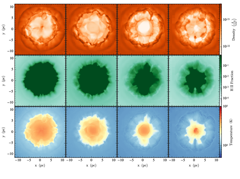
Figure 1.— Slices of M4N3E8mod at $t=5.75$ (burst of accretion), 5.82, 5.88, and 5.95 Myr from left to right panels. The top, middle, and bottom panels show gas density, H ii fraction, and gas temperature, respectively. Due to the inhomogeneity of the gas, the Strömgren radius is approximately spherically symmetric but with a large variation in distances from the BH. At peak accretion rate the Strömgren radius reaches its maximum size, which can also be seen in the temperature slices. As the accretion rate decreases (from left to right), the H ii region shrinks but never vanishes.

II.2. Radiation-Hydrodynamic Simulations with Enzo+Moray

We perform local 3D radiation-hydrodynamic simulations in Cartesian coordinates using the AMR code Enzo coupled with the adaptive ray tracing module Moray (Wise & Abel, 2011; Bryan et al., 2014).

The BH is modeled as a sink particle and is located at the center of the computation domain. We fix the position of the BH throughout the simulation and update the BH mass to account for growth through accretion. We assume a simple initial condition of uniform temperature and density, as well as zero velocity and metalicity for the background gas (see Yajima et al., 2017, for dusty accretion onto BHs). We assume an adiabatic gas ($\gamma=5/3$) and neglect its self-gravity. We select $M_{\rm BH}=10^{4}\,M_{\sun}$, $n_{\infty}=10^{3}\,{\rm cm}^{-3}$, and $T_{\infty}=10^{4}$ K as the baseline setup in the feedback-dominated regime (Park & Ricotti, 2012). Note that the combination of $M_{\rm BH}$ and $n_{\infty}$ can be extended to other sets of simulations which return qualitatively comparable results (i.e., Equation (7) holds and the size of H ii region is $\propto M_{\rm BH}$) when $M_{\rm BH}\,n_{\infty}$ is kept constant. Table 1 lists the parameters for each simulation. We use the following naming convention for simulations: runs are denoted as ‘MmNn’ where the BH mass is $M_{\rm BH}=10^{m}\,M_{\sun}$ and gas number density is $n_{\infty}=10^{n}\,{\rm cm}^{-3}$.

We use numerical resolution of $32^{3}$ on the top grid in most of our simulations, except where noted otherwise. This resolution corresponds to a coarsest resolution element with the size, $\Delta L_{\rm max}$, listed in Table 1. With 3 levels of refinement our simulations attain the finest resolution of $\Delta L_{\rm min}=0.156(M_{\rm BH}/10^{4}\,M_{\sun})\,$pc. The strategy we adopt for AMR is to achieve the highest level of resolution both in the central region near the BH and around the ionization front. In order to accomplish this, we enforce the highest level of refinement within the box of a size $\Delta L_{\rm max}$ centered around the BH (see Table 1). In addition to this requirement we also use the local gradients of all variables (i.e., density, energy, pressure, velocity, and etc) to flag cells for refinement around the ionization front. Outflowing boundary conditions are imposed on all boundaries to prevent reflection of density waves, which form due to the expansion of the ionized region.

We use the non-equilibrium chemistry model for $\rm H\,{\textsc{i}}$, $\rm H\,{\textsc{ii}}$, ${\rm He}\,\textsc{i}$, ${\rm He}\,\textsc{ii}$, ${\rm He}\,{\textsc{iii}}$, and $e^{-}$ implemented in Enzo (Abel et al., 1997; Anninos et al., 1997). For simplicity, we consider the photo-heating and cooling of pure hydrogen gas and neglect the effects of radiation pressure, which are relatively minor. The radiation pressure on both the electron gas and neutral hydrogen is weaker than the local gravity by the BH and negligible relative to the thermal pressure which plays a central role in creating outflows inside the H ii region (see Park & Ricotti, 2012, for details). The photo-heating of the hydrogen-helium gas mixture is known to return a higher temperature inside the H ii region (i.e., $T_{\rm HII}\sim 6\times 10^{4}$ K), which leads to somewhat lower accretion rate and qualitatively similar results to the pure hydrogen gas. The Compton heating plays a minor role compared to the photo-heating when the radiation spectrum is soft (Park et al., 2014b) and is therefore neglected.

Radiation emitted from the innermost parts of the BH accretion flow is propagated through the computational domain by the module Moray, which solves radiative transfer equation coupled with equations of hydrodynamics. Specifically, Moray accounts for the photo-ionization of gas and calculates the amount of photo-heating, which contributes to the total thermal energy of the gas. Moray uses adaptive ray tracing (Abel & Wandelt, 2002) that is based on the HEALPix framework (Górski et al., 2005). In this approach the BH is modeled as a radiation point source that emits $12\times 4^{3}$ rays which are then split into four child rays so that a single cell is sampled by at least 5.1 rays. The adaptive ray splitting occurs automatically when the solid angle associated with a single ray increases with radius or if the ray encounters a high resolution AMR grid. The radiation field is updated in every time step that corresponds to the grid with the finest numerical resolution as set by the Courant-Friedrichs-Lewy condition.

II.3. Modified power-law spectral energy distribution

We describe the accretion luminosity with a power law spectrum, $L_{\nu}=C\nu^{-\alpha}$, where $\alpha$ is the spectral index and $C$ is the normalization constant. The frequency integrated (bolometric) luminosity between the energy $h\nu_{1}$ and $h\nu_{2}$ is $L_{\rm acc}=C(\nu_{2}^{1-\alpha}-\nu_{1}^{1-\alpha})/(1-\alpha)$ for $\alpha\neq 1$. Moray models the SED with $N_{\nu}=4-8$ discrete energy bins that are equidistant in log-space between $E_{\rm min}=h\nu_{\rm min}=13.6$ eV and $E_{\rm max}=h\nu_{\rm max}=100$ keV. A fraction of energy is allotted to each bin assuming the spectral index $\alpha=1.5$. The mean photon energy of the $n$-th bin $\langle E_{n}\rangle$ between energies $E_{n-1}$ and $E_{n}$ is calculated as

$$\langle{E}_{n}\rangle=\frac{\alpha}{\alpha-1}\frac{(E_{n}^{1-\alpha}-E_{n-1}^{1-\alpha})}{(E_{n}^{-\alpha}-E_{n-1}^{-\alpha})}\,\,{\rm for}\,\,\alpha>1$$ (8)

which returns the mean energy of $\langle E\rangle\simeq 40.3$ eV for the entire energy range. Table 2 lists the mean energy ($h\nu_{n}$) and the dimensionless fraction of bolometric luminosity allotted to each bin ($L_{n}$). The number of ionizing photons in each bin is then calculated as $L_{n}L_{\rm acc}/\langle{E}_{n}\rangle$.

The prescription for modeling the spectrum outlined above ensures that the total power of emitted radiation is divided among the chosen number of energy bins to model the SED. In addition to the energy spectrum of radiation, another crucial consideration for radiation transport is the number of ionizing photons contained in each energy bin, as given by the photon spectrum. In order to maintain consistency in terms of the photon spectrum among simulations with different values of $N_{\nu}$, we introduce a modification to the number of photons in the first energy bin. This ensures that the number of near-UV ionizing photons, which are responsible for the bulk of photo-ionizations and photo-heating, remains approximately the same regardless of which SED model is used. Specifically, the mean energy of the lowest energy bin determines the temperature of H ii region, which is why we adopt the same energy of $E_{1}=28.4$ eV for 4 and 8-bin SED models (the original first entry for $N_{\nu}=8$ is $E_{1}=21.5$ eV). The fraction of energy in this bin is accordingly adjusted from 0.4318 to 0.5704 so to preserve the same number of ionizing photons. One consequence of this optimization performed simultaneously in terms of the luminosity and number of ionizing photons is that the sum of luminosity fractions allotted to all energy bins ($L_{n}$) is no longer exactly equal to 100%, as can be seen from Table 2. We choose the 4-bin model without modification as a reference since it still returns a consistent result with Park & Ricotti (2011) using the minimum number of energy bins.

In the Appendix we include a detailed discussion of the SED optimization used in this work, along with convergence tests, and a comparison with SED models published in Mirocha et al. (2012). We explore a full set of modeled SEDs in our simulations and mark those that are modified as outlined in this section in Table 1. For example, ‘E8mod’ indicates the case of modified SED with 8 energy bins and ‘sec’ marks the case with secondary ionizations included to consider the effect by energetic particles produced by high energy X-ray photons.

Table 2SEDs for Power-law BH radiation with $\alpha=1.5$

$n_{\nu}$	$N_{\nu}=4$	$N_{\nu}=8$
1	(28.4, 0.6793)	(28.4, 0.5704)
2	(263.0, 0.2232)	(65.3, 0.2475)
3	(2435.3, 0.0734)	(198.7, 0.0813)
4	(22551.1, 0.0241)	(604.5, 0.0813)
5	…	(1839.5, 0.0466)
6	…	(5597.8, 0.0267)
7	…	(17034.3, 0.0153)
8	…	(51836.1, 0.0088)

III. Results

Our 3D simulations are characterized by the oscillatory behavior of the accretion rate and size of ionized region, which is analogous to the previous 1D/2D simulations. Our simulations also show the presence of the turbulent gas motion driven by the fluctuating ionized region, which has not been captured in lower dimensionality simulations.

III.1. Formation of ionized region and oscillatory behavior

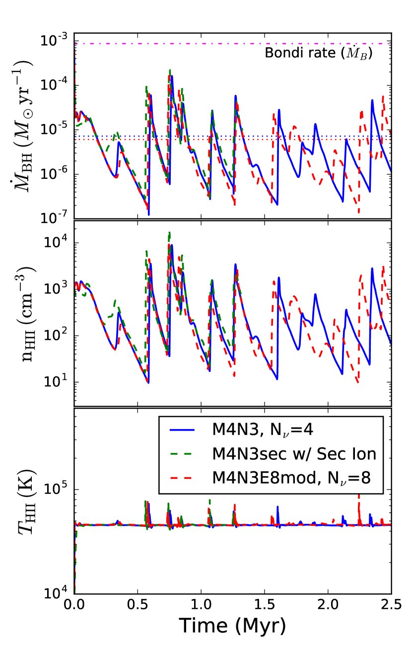
Figure 2.— From top to bottom: accretion rate onto the BH (with mean values shown as dotted lines), density and temperature inside the H ii region near the BH for the runs M4N3 (blue solid), M4N3sec (green dashed), and M4N3E8mod (red dashed). The accretion rate exhibits oscillatory behavior and spans $\sim$ 3 orders of magnitude between the maximum ($\sim 10^{-4}\,{\rm M}_{\odot}/{\rm yr}$) and minimum ($\sim 10^{-7}\,{\rm M}_{\odot}/{\rm yr}$). Dot-dashed line shows the Bondi rate ($\dot{M}_{\rm B}$) for neutral gas with $T_{\infty}=10^{4}$ K.

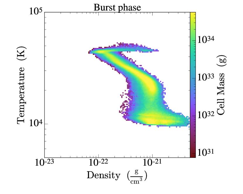
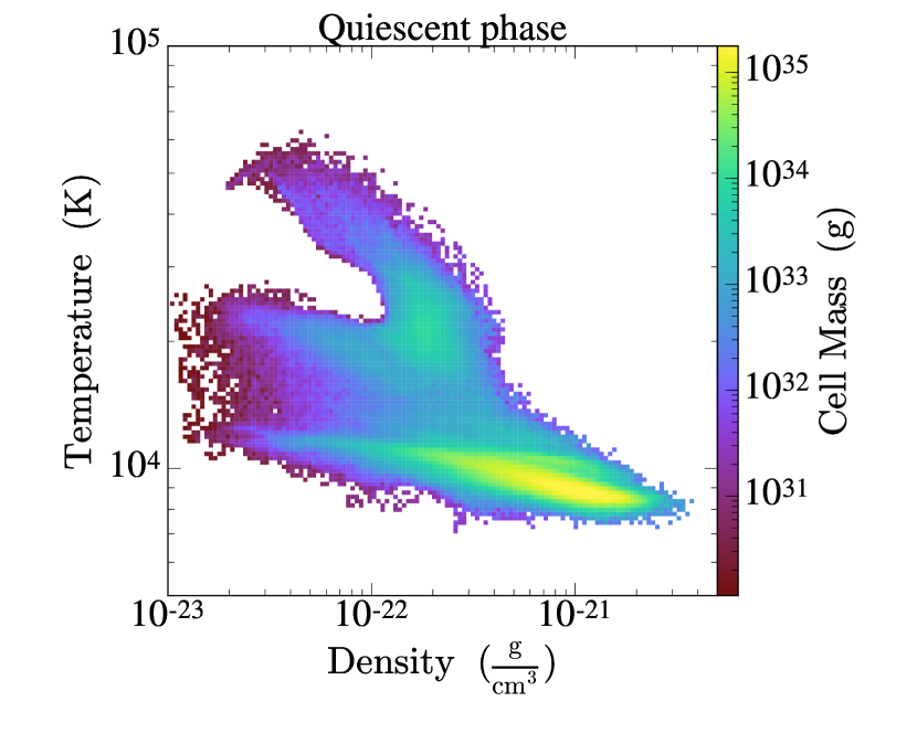
Figure 3.— Gas density and temperature distribution in M4N3E8mod run during the accretion burst (left) and quiescent (right) just before the subsequent burst within the central 8 pc. Color marks the cumulative mass of the gas contributing to each cell of the phase diagram.

Figure 1 shows the evolution of the gas density (top), H ii fraction ($n_{\rm HII}/n_{\rm H}$, middle), and temperature (bottom) for the M4N3E8mod run. From left to right the snapshots illustrate evolution of the ionized region starting with the burst of accretion and ending with a quiescent phase just before the subsequent burst. In general, the region under the influence of ionizing radiation is characterized by the low gas density, high ionization fraction, and high temperature ($T\sim 4\times 10^{4}$ K).

The low density Strömgren sphere roughly maintains spherical symmetry throughout a sequence of oscillations despite a highly turbulent nature of the gas between the high and low density regions separated by the ionization front. In contrast to the turbulent features imprinted in the density map shown in the top panels of Figure 1, the H ii fraction and temperature maps are relatively uniform. All maps illustrate a correlation of the size of the Strömgren sphere with the accretion rate: as the accretion rate decreases (from left to right), the average size of Strömgren sphere also decreases. Unlike the 1D/2D simulations however, in 3D simulations the Strömgren sphere never completely collapses between the accretion outbursts.

The outline of the H ii region traced by the H ii fraction and temperature shows a more dramatic departure from spherical symmetry than the smoother density maps. The “jagged” edge of the H ii region can be directly attributed to ionization of gas by the UV photons. It arises as a consequence of inhomogeneity of the gas driven by turbulence, which produces a range of column densities along different radial directions, as seen by the central source. More energetic photons with longer mean free paths travel beyond the ionization front of the H ii region partially ionizing the gas there. Their effect is noticeable in the H ii fraction maps as a light green halo surrounding the ionization front, size of which remains approximately constant regardless of the accretion phase.

III.2. Accretion rate and period of oscillation

The top panel of Figure 2 shows evolution of the accretion rate, which is calculated from the gas density (middle), and gas temperature (bottom), for the runs M4N3 (blue solid), M4N3sec (green dashed), and M4N3E8mod (red dashed). The temperature of the ionized region, $T_{\rm HII}$, increases modestly during the accretion bursts and consequently, does not play a large role in determining the accretion rate onto the BH. It follows that the density of the ionized region, which varies by a few orders of magnitude, is the primary driver of evolution of the accretion rate.

Indeed, the amplitude and variability of the accretion rate in Figure 2 closely follow the density of the ionized gas, as expected given the adopted prescription of the Bondi accretion rate, $\dot{M}_{\rm BH}\propto\rho_{\rm HII}$. A notable departure of the 3D simulations is that the accretion rate spans the range of 2-3 orders of magnitude compared to the 1D/2D simulations, where this range is measured to be 5-6 orders of magnitude (Park & Ricotti, 2011, 2012). The difference seen in the 3D simulations can be directly attributed to a higher level of “quiescent” accretion that occurs between the outbursts, while the maximum and mean accretion rate remain approximately unchanged relative to the 1D/2D models. In the case of 1D/2D simulations, a sharp density drop inside of the ionization front is well preserved until the front collapses to a very small radius. The relatively high gas density inside the ionization front in the 3D simulations, explains the higher level of accretion rate during the quiescent phase. The difference between the current 3D and former 1D/2D simulations may arise due to different dimensionality of simulations, however we cannot completely rule out a possibility that the difference in the codes and numerical schemes are also partially responsible.

We also investigate the effect of modified spectrum of the ionizing source as well as that of secondary ionizations by more energetic X-ray photons which generate energetic particles causing further ionization. Specifically, in addition the baseline run M4N3, we carry out the run M4N3sec, which accounts for secondary ionizations and M4N3E8mod, which uses our modified prescription for the ionizing continuum modeled in 8 energy bins. We find consistent results for all three. Based on this we conclude that (a) secondary ionizations do not have a significant impact on the thermodynamic state of the gas and (b) that our prescription for the ionizing continuum in M4N3E8mod returns physical results indistinguishable from the baseline simulation (see Appendix for more discussion of the latter).

In addition to the peak and mean accretion rates, the mean period between the bursts of accretion (i.e., the accretion duty cycle) is consistent with the previous 1D/2D results. The mean accretion rate (dotted lines) for all M4N3 runs is approximately 2 orders of magnitude lower than the Bondi rate for neutral gas (dot-dashed line). The mean period between the bursts is approximately $0.25\,$Myr, consistent with earlier results of Park & Ricotti (2011, 2012)

$$\tau_{\rm cycle}\sim 0.22\,{\rm Myr}\left(\frac{M_{\rm BH}}{10^{4}\,M_{\sun}}\right)^{\frac{2}{3}}\left(\frac{n_{\infty}}{10^{3}\,{\rm cm^{-3}}}\right)^{-\frac{1}{3}}$$ (9)

with $\alpha=1.5$ and $\eta=0.1$ for radiative efficiency.

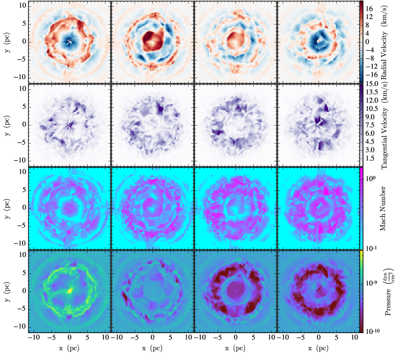
Figure 4.— From top to bottom: slices of radial velocity, tangential velocity magnitude, Mach number, and thermal pressure in run M4N3E8mod, respectively. The times for each snapshot match those shown in Figure 1.

III.3. Phase diagrams and velocity structure

Figure 3 shows the phase diagrams of the gas density and temperature during the burst (left) and quiescent (right) phases for M4N3E8mod run. The plotted values of density and temperature are measured within 8 pc radius surrounding the BH (see Figure 1). During the bursts, the gas in vicinity of the BH is photo-ionized and photo-heated to $T\approx 5\times 10^{4}\,$K, as illustrated by a horizontal branch in the $T-\rho$ distribution. The rest of the gas in the outer part of Strömgren sphere is shown as a separate branch, characterized by temperature decreasing with density. This temperature structure is consistent with Figure 1 where the central region shows a fairly uniform temperature, which then decreases with radius at larger separations from the BH.

During the quiescent phase, most of the gas cools through recombination to $T\approx 10^{4}\,$K. However, a smaller fraction of high temperature, low density gas still appears in the same location at the top left corner of the diagram, giving rise to a relatively wide multi-phase distribution of gas. Note that in 1D/2D simulations, the central region is replenished with high density gas during the quiescent phase as the ionization front collapses to the minimum size, which is significantly smaller than the size of the H ii region on average (Milosavljević et al., 2009; Park & Ricotti, 2011). In 3D simulations, even though the ionization front does not collapse entirely during the quiescent phase (i.e., the radius of H ii bubble remains approximately half the average size), the enhanced gas density within the ionized region is still sufficient to trigger the next burst of accretion. The reason why the hot bubble maintains larger size during the quiescent phase in 3D simulations is related to the higher accretion rate and enhanced gas density just inside the ionization front, as explained in the previous section.

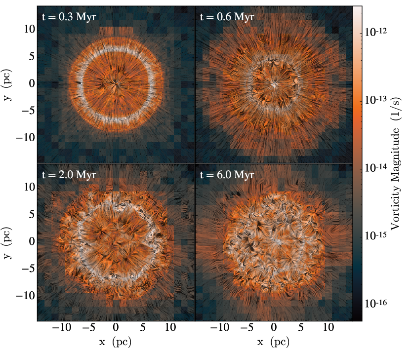
Figure 5.— Evolution of vorticity magnitude, $|\vec{\omega}|$, in run M4N3E8mod at $t=$ 0.3, 0.6, 2.0, 6.0 Myr over-plotted with the line integral convolution of velocity field (Cabral & Leedom, 1993) where the texture visualizes the local direction of the velocity field. The vorticity builds up over time but saturates during the early phase of the simulation.

Figure 4 shows the radial velocity, tangential velocity magnitude, Mach number, and thermal pressure in run M4N3E8mod during the same phases shown in Figure 1. During the burst of accretion (first column), the gas in the central region falls into the BH boosting the accretion rate while a strong outflow (colored in red) is still observed in the outer part of the ionized region at $r\sim 5$ pc. The outflow velocity reaches $\sim 20$ km/s, the transonic value for the temperature of the ionized region, as illustrated by the Mach number slices.

As the transonic gas outflow encounters the neutral medium, the kinetic energy of the gas is efficiently dissipated by shocks. The supersonic gas is mostly found near the ionization front or just outside of the Strömgren sphere. The central core shows the highest thermal pressure during the burst of accretion due to the high density of the core but the temperature distribution within the ionized region remains uniform, as shown in Figure 1. A spherical shell around the ionization front also exhibits high thermal pressure because the neutral clumps of gas in this region are efficiently photo-heated by the ionizing UV photons that escape absorption by the central core.

After the burst, the central region starts to develop an outflow (second and third columns) driven by the high thermal pressure. The high thermal pressure, located at the core and around the ionization front in the first column, expands and dissipates as the accretion powered luminosity decreases in time. The average thermal pressure is maximal during the burst (first column) and decreases as a function of time displaying the minimum just before the subsequent burst (last column). The inner region becomes gradually under-pressurized due to expansion and radiative cooling. This allows the gas to flow toward the center, causing a subsequent accretion burst.

The velocity structure in this work is distinct from the 1D/2D simulations where a strong laminar (i.e., non-turbulent) outflow in the outer part of the Strömgren sphere persists most of the time. In these simulations the ionization front collapses completely due to the loss of thermal pressure in the ionized region. The 3D simulations described here instead show highly turbulent motion in both radial (first row) and tangential directions (second row) that cascades to small scales over several oscillation cycles. The tangential velocity is only suppressed in the central region during the strong inflow and outflow episodes.

III.4. Evolution of vorticity

We use vorticity, defined as a curl of the velocity field

$$\vec{\omega}=\vec{\nabla}\times\vec{v}$$ (10)

to quantify the degree of turbulent motion of the gas. Figure 5 shows the evolution of vorticity at times 0.3, 0.6, 2.0, and 6.0 Myr in the run M4N3E8mod. The line integral convolution (Cabral & Leedom, 1993), a method to create a texture correlated in the direction of the vector field, is shown in black over vorticity magnitude. The vorticity is highest around the ionization front and propagates inward and outward. It builds up over time and saturates during the early phase of the simulation, at $t=2.0\,$Myr, after which point it does not display a significant increase until $t=6.0\,$Myr.

The propensity of the gas to develop turbulence in 3D simulations can be understood in the context of the vorticity equation, which written as Lagrangian derivative ($D/Dt$) reads

$$\frac{D\vec{\omega}}{Dt}=\frac{\partial\vec{\omega}}{\partial t}+(\vec{v}\cdot\nabla)\vec{\omega}=\frac{1}{\rho^{2}}\nabla\rho\times\nabla p.$$ (11)

The right hand side of the equation quantifies the baroclinicity of a stratified fluid, present when the gradient of pressure is misaligned from the density gradient of the gas. In our simulations, the local density gradients have no preferred direction because of the turbulence which produces a significant inhomogeneity of density, as evident in Figure 1. On the other hand, the pressure gradient is generally along the direction of gravity and largest across the ionization front. This misalignment dictates the evolution of $\vec{\omega}$ close to the ionization front.

From dimensional analysis the magnitude of vorticity squared can be estimated as $|\vec{\omega}|^{2}\sim GM_{\rm BH}/r^{3}$, where the relevant radius corresponds to the size of the Strömgren sphere. The number of ionizing photons from the BH is proportional to the density squared from recombination rate as well as the recombination volume, $N_{\rm ion}\propto\langle R_{s}\rangle^{3}n_{\infty}^{2}$ where $\langle R_{s}\rangle$ is the mean size of the Strömgren radius. On the other hand $N_{\rm ion}$ is also proportional to the Bondi accretion rate, i.e., $N_{\rm ion}\propto M_{\rm BH}^{2}n_{\infty}$ (Park & Ricotti, 2011). Thus, the mean size of Strömgren sphere is related to the BH mass and gas density as $\langle R_{s}\rangle^{3}n_{\infty}^{2}\propto M_{\rm BH}^{2}n_{\infty}$. Using this in the estimate of the mean magnitude squared, $|\vec{\omega}|^{2}$, which develops around the ionization front

$$\left|\vec{\omega}\right|^{2}\sim\frac{GM_{\rm BH}}{\langle R_{s}\rangle^{3}}\propto\frac{n_{\infty}}{M_{\rm BH}}.$$ (12)

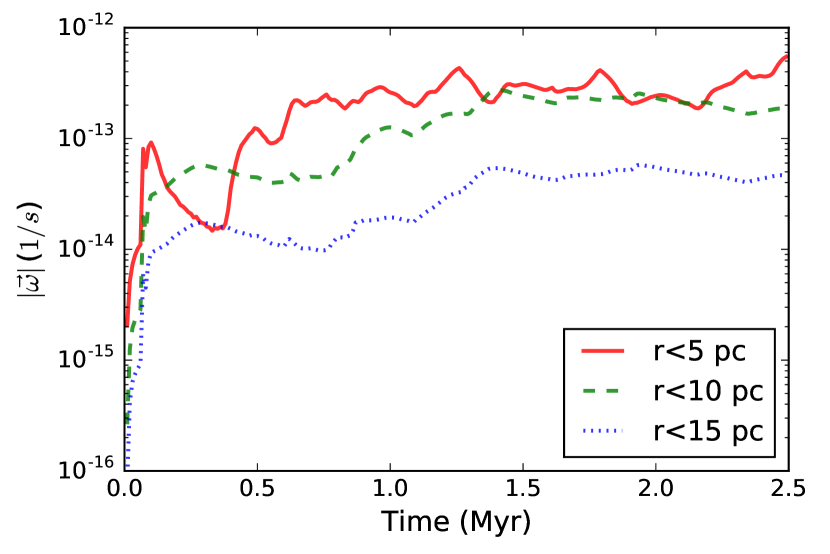
Figure 6.— Time evolution of the mass-weighted mean vorticity $|\vec{\omega}|$ for run M4N3, calculated within the radius $r=5$, 10, and 15 pc.

Figure 6 shows the time evolution of mass-weighted mean vorticity $|\vec{\omega}|$ for the simulation M4N3, calculated within the radius $r=5.0$ (solid line), 10.0 (dashed), and 15.0 pc (dotted). On average, mean vorticity shows a rapid increase at the beginning at all radii and remains at a constant level after $t\approx 1.3$ Myr. For the $r<5.0$ pc volume, the vorticity shows a significant change during the initial phase ($t\lesssim 0.5$ Myr) , when the ionization front crosses this scale, but reaches a steady value with a minor variation after only $t\gtrsim 1$ Myr. The small variation in $|\vec{\omega}|$ for the $r<5.0$ pc volume shows an approximate match with the accretion cycles in Figure 2. On the other hand, $|\vec{\omega}|$ for the volumes with $r<10.0$ pc and $<15.0$ pc show a steady increase until $t\approx 1.3$ Myr and remains at the same level after that. Note that for the run M4N3 the ionization front extends to a radius of $r\approx 10$ pc as shown Figure 1, thus $r\approx 10$ pc volume is large enough to capture most of the vorticity. The value of $|\vec{\omega}|$ for $r<5.0$ pc and $r<10.0$ pc volumes after $\gtrsim 1.3$ Myr becomes comparable, which means that there is no noticeable difference in $|\vec{\omega}|$ in inner and outer parts of the ionized region. However, as we increase the volume, i.e., $r<15.0$ pc, the mean $|\vec{\omega}|$ decreases since the volume outside of ionized region with low $|\vec{\omega}|$ is included.

Figure 7 shows the evolution of the mean vorticity squared for simulations M4N3 (solid red, 5 pc), M4N4 (dashed blue, 2.5 pc), and M6N1 (dashed green, 0.5 kpc) within the radius written in parentheses for each run. The selected radius is approximately a half of the mean Strömgren radius $\langle R_{s}\rangle$ for each. To show all three simulations on the same scale, we normalize $\left|\vec{\omega}\right|^{2}$ by $n_{\infty}M_{\rm BH}^{-1}$, as in Equation (12), and the time on the $x$-axis by the average length of the oscillation cycle $\propto M_{\rm BH}^{2/3}n_{\infty}^{-1/3}$ shown in Equation (9). Note that simulations M4N3 and M6N1 which share the same value of $M_{\rm BH}n_{\infty}=10^{7}\,M_{\sun}{\rm cm}^{-3}$, display a good match while M4N4 shows a reasonably consistent result considering the large range of $\left|\vec{\omega}\right|^{2}$.

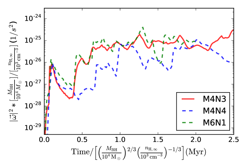
Figure 7.— Evolution of the mass-weighted mean vorticity squared for runs M4N3 (solid red), M4N4 (dashed blue), and M6N1 (dashed green) calculated within the radius of $0.5\langle R_{s}\rangle$. $|\vec{\omega}|^{2}$ is normalized by $n_{\infty}/M_{\rm BH}$ and time is in units of $(M_{\rm BH}^{2}/n_{\infty})^{1/3}$ (see text for more details).

III.5. Turbulent Kinetic Energy

In order to quantify how much turbulent energy is present on different spatial scales we calculate the energy spectrum $E(k)$ as a function of the wavenumber $k$. The total turbulent kinetic energy per unit mass is evaluated as

$$\frac{1}{2}\left<|\vec{v}|^{2}\right>=\int_{0}^{\infty}E(k)dk$$ (13)

where $\vec{v}$ shown here only accounts for the turbulent component of the velocity.

Figure 8 shows the specific turbulent kinetic energy power spectrum from runs M4N3R32 (top) and M4N3E8R64mod (bottom), plotted for phases of an accretion cycle at $t\sim 1.3$ Myr after which the mean vorticity reaches at a steady value as shown in Figure 6. The wavenumber is defined as $k=1/\Delta L$, where $\Delta L$ corresponds to the scale ranging from the finest resolution element to the size of the entire computational domain. In calculations presented here $\Delta L$ (and hence, $k$) is expressed in code units while $E(k)$ is shown in ${\rm cm}^{2}/{\rm s}^{2}$. The shaded region defined by $R_{\rm s,max}$ and $R_{\rm s,min}$, which represent the maximum and minimum sizes of the Strömgren radius, marks the scale for the turbulence source. $\Delta L_{\rm max}$ and $\Delta L_{\rm min}$ indicate the resolutions of the top and finest grids, respectively. Note that the high resolution run M4N3E8R64mod is characterized by a wider range of k which extends to larger values, resulting in a better resolved turbulence at small spatial scales.

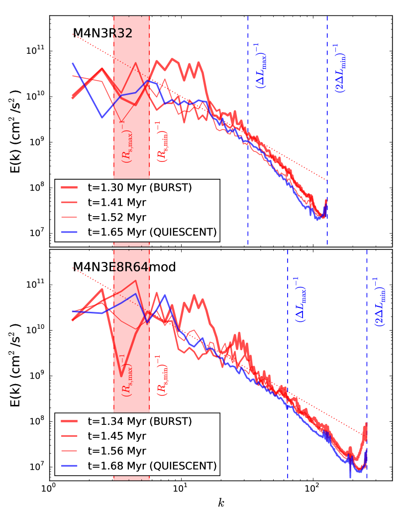
Figure 8.— Power spectrum of the specific turbulent kinetic energy at different times during one accretion cycle in simulation M4N3R32 (top) and M4N3E8R64 (bottom). $R_{\rm s,max}$ and $R_{\rm s,min}$ are the maximum and minimum radius of the Strömgren sphere and $\Delta L_{\rm max}$ and $\Delta L_{\rm min}$ are the sizes of the coarsest and the finest resolution element, respectively. The dotted line traces the Kolmogorov spectrum with the slope $E(k)\propto k^{-5/3}$.

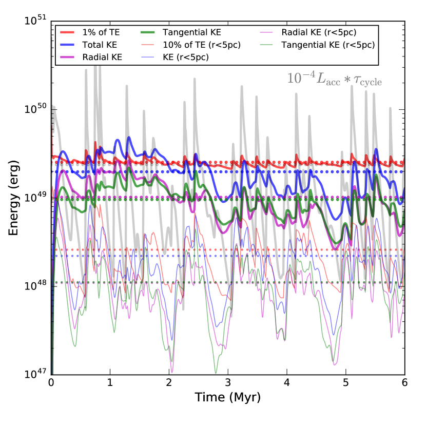
Figure 9.— Evolution of the total thermal (red) and kinetic (blue) energy for M4N3E8. Gray line shows the energy in radiation emitted from the BH during one cycle of oscillation (i.e., $L_{\rm acc}*\tau_{\rm cycle}$). Kinetic energy is decomposed into radial (magenta) and tangential (green) components. Horizontal dotted lines indicate mean values for each energy component. Thick and thin lines show the energies in the entire volume and within the sphere with radius $r=5$ pc, respectively.

The turbulence is sourced on the scales that are just inside the ionization front ($k\lesssim 6$) and it cascades to smaller scales (larger $k$). Figure 8 illustrates that in quiescence (blue line) the turbulent energy tends to be slightly lower across the spectrum relative to the other phases of the accretion cycle. The turbulent energy spectrum calculated from simulations is broadly consistent with the Kolmogorov spectrum [$E(k)\propto k^{-5/3}$; Kolmogorov (1991)], which provides analytic description of a saturated and isotropic turbulence. Departure from the Kolmogorov spectrum is noticeable in two spatial regions in Figure 8. Namely, the turbulence is diminished in neutral gas, outside of the ionization sphere, which is consistent with our hypothesis of radiatively driven turbulence. Secondly, the simulated spectrum departs from Kolmogorov at wave numbers $k\gtrsim 30$ for M4N3R32 and $k\gtrsim 60$ for M4N3E8R64mod, respectively, that correspond to scales smaller than $\Delta L_{\rm max}$. Note that the inertial regime where $E(k)\propto k^{-5/3}$ is extended to larger $k$ for M4N3E8R64mod whereas the dissipation regime arises at $k\gtrsim\Delta L_{\rm max}^{-1}$ consistently for both simulations with different resolutions. This region coincides with a portion of a simulation domain where we employ several different refinement levels in the form of layered grids. Specifically, while the highest level grid resolves eddies of the size $2\Delta L_{\rm min}$, the base grid will resolve eddies with the minimum size of $\Delta L_{\rm max}=8\Delta L_{\rm min}$. Because of the non-uniform sampling of turbulence in these regions some fraction of the turbulent kinetic energy is numerically dissipated before it cascades to the smallest scales. This expectation is consistent with the spectrum that steepens towards smallest scales (highest $k$ numbers), as shown in the figure. The turbulent kinetic energy contained on small scales is however a small fraction of the total turbulent kinetic energy and we do not expect that numerical dissipation of turbulence into the internal energy of the gas will significantly affect gas thermodynamics on these scales.

Figure 9 summarizes contribution to the total energy budget of the simulated gas flow from the accretion powered radiation, thermal and kinetic energy of the gas in run M4N3E8. We find that the average energy of radiation in one accretion cycle, $\langle L_{\rm acc}\,\tau_{\rm cycle}\rangle\sim 2.4\times 10^{53}\,$erg, dominates over all other components of energy by more than $\sim$ 2 orders of magnitude. The energy of radiation is estimated as the bolometric luminosity emitted from the BH multiplied by a characteristic length of one cycle of oscillation and is plotted as a gray line. This implies that radiation can easily drive turbulence and account for the increased internal energy of the gas, as energetic requirements for these are comparatively modest.

The remaining components of energy are the thermal energy of the gas (TE), marked as red line in Figure 9, and the kinetic energy (KE), marked as blue line. Because the relative contributions to thermal and kinetic energy are different for the strongly irradiated gas in vicinity of the BH and neutral gas outside of the Strömgren sphere, we show the evolution of TE and KE in the entire computational domain as well as within the sphere with radius $r=5$ pc. Recall that in the run M4N3E8 the ionization front resides at a radius of $r\approx 10$ pc, and so the volume within $r<5$ pc traces plasma enclosed within the Strömgren sphere at all times.

The kinetic energy is a combination of the kinetic energy of the bulk flow (i.e., the radial inflow and outflow of the gas) combined with random motions of the gas due to turbulence. The total kinetic energy is calculated from simulations as

$${\rm KE}=\frac{1}{2}\Sigma m_{i}(v_{i,x}^{2}+v_{i,y}^{2}+v_{i,z}^{2})$$ (14)

where $m_{i}$ is the cell mass and $v_{i,x}$, $v_{i,y}$, and $v_{i,z}$ are the velocity components in x, y, and z directions, respectively. The average energies (horizontal dotted lines) show that the kinetic energy (thick blue) is equivalent to $\sim 1\,\%$, of the thermal energy (thick red) in the entire computation domain. Similarly, kinetic energy corresponds to $\sim 7\,\%$ of the thermal energy for the gas within $r<10$ pc and to $\sim 9\,\%$ for the gas within $r<5$ pc (the latter is shown with thin lines). Therefore, the kinetic energy of the gas corresponds to less than 10% of the thermal energy anywhere in the computational domain. It then follows that the kinetic energy due to turbulence cannot be the main contributor to the pressure support of the gas, which is mostly provided by thermal pressure. Along similar lines, even if all kinetic energy of the gas is promptly thermalized, it would not significantly alter the internal energy of the gas. This is the basis for our earlier statement that numerical dissipation of turbulence due to finite spatial resolution should not affect thermodynamics of the gas.

In order to estimate the contribution to the total kinetic energy from the bulk flow and turbulence we initially decompose the kinetic energy into the radial and tangential components, shown as magenta and green lines in Figure 9, respectively. Specifically, we calculate the radial component as KE${}_{\rm R}=\Sigma m_{i}v_{i,r}^{2}/2$, where $v_{i,r}$ is the radial velocity, and the tangential component as KE_T= KE - KE_R. Figure 9 shows that shortly after the beginning of the simulation the two components achieve equipartition and KE_R $\approx$ KE_T. Because the bulk flow of the gas is mostly along the radial direction, KE_R actually accounts for both the kinetic energy of the bulk flow and turbulence. The KE_T component of kinetic energy is on the other hand mostly contributed by turbulence. We estimate the magnitude of the turbulent component of kinetic energy in radial direction as $\sim$ 1/2 KE_T, given that turbulence is isotropic, so that tangential and radial motions account for two and one degrees of freedom, respectively. It follows that the total kinetic energy is KE = KE_bulk + 3KE_T/2 and because KE_R $\approx$ KE_T, the turbulent kinetic energy contributes $\sim$ 3/4 of the total kinetic energy. Therefore, turbulent motions on all scales dominate the kinetic energy of the entire accretion flow.

IV. Discussion and Conclusions

The main aim of this paper is to extend numerical studies of accretion mediated by radiative feedback to full 3D local simulations and identify physical processes that have not been captured by the local 1D/2D models. We achieve this by performing 3D simulations of radiation-regulated accretion onto massive BHs using the AMR code Enzo equipped with the adaptive ray tracing module Moray (Wise & Abel, 2011). Our main findings are listed below.

• Our 3D simulations corroborate the role of ionizing radiation in regulation of accretion onto the BHs and in driving oscillations in the accretion rate. We also confirm the mean accretion rate and the mean period between accretion cycles found in earlier studies (Park & Ricotti, 2011, 2012). Since this study adopts different code and numerical schemes relative to the earlier ones, this provides verification that 3D simulations described here accurately reproduce the key features of 1D/2D models.

• The 3D simulations show significantly higher level of accretion during the quiescent phase due to the enhanced gas density within the ionization front and thus oscillations in the accretion rate of only $\sim 2-3$ orders of magnitude in amplitude, significantly lower than in 1D/2D models. We caution however that even though 3D simulations seem to faithfully reproduce the 1D/2D simulations, we cannot fully rule out a possibility that higher level of accretion during quiescence is caused by differences in the numerical scheme employed in this work.

• In terms of the energy budget of the gas flow, we find that the radiative energy dominates over the thermal and kinetic energy of the gas by more than $\sim$ 2 orders of magnitude, implying that radiation can easily drive turbulence and account for the increased internal energy of the gas. The thermal energy of the gas dominates over the kinetic energy by a factor of $\sim 10-100$ depending on the distance from the BH, while the kinetic energy itself is mostly contributed by the turbulent motions of the gas. The turbulence therefore does not contribute significantly to the pressure support of the gas.

The local simulations of radiation feedback mediated accretion onto BHs presented here are the first step towards investigation of the full 3D phenomena that take place in vicinity of growing BH. Future, more sophisticated local 3D simulations will in addition to turbulence need to capture the physics of magnetic fields, angular momentum of gas, and anisotropy of emitted radiation. All these ingredients are likely to play an important role in determining how quickly BHs grow and how they interact with their ambient mediums.

This study also bridges the gap between the local and cosmological simulations. In large cosmological simulations radiative feedback from BHs is often treated as purely thermal feedback and calculated without directly solving the radiative transfer equations. This is a practical compromise because direct calculations of radiative transfer are still relatively computationally expensive, albeit not impossible. This study paves the way for the next generation of cosmological simulations in which the BH radiative feedback will be evaluated directly. It remains to be explored how the rich phenomena discovered in local simulations will affect the details of the growth and feedback from BHs at the centers of galaxies or BHs recoiling during galaxy mergers (e.g., Sijacki et al., 2011; Souza Lima et al., 2017; Park & Bogdanović, 2017).

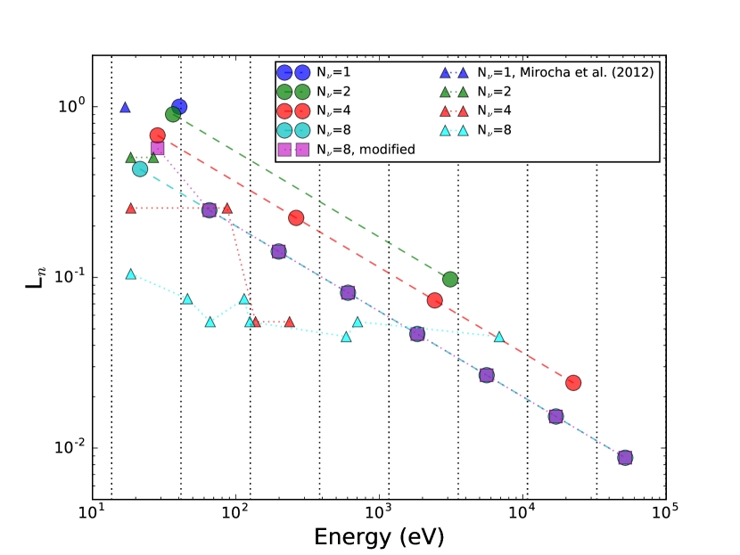
Figure 10.— Spectral energy distribution for a power-law spectrum with $\alpha=1.5$ with different number of energy bins $N_{\nu}=1,2,4$, and 8. To match the $N_{\nu}=8$ case to $N_{\nu}=4$, the first energy bin is shifted from 21.5 eV to 28.4 eV which matches the energy for the case $N_{\nu}=4$. We also modify the fraction of allocated energy for this bin from 0.4318 to 0.5704 so that the number of total ionizing photons remains constant. Triangles show the optimized SEDs using the method by Mirocha et al. (2012).

Modeling of the Power-law Spectral Energy Distribution

We find that simulations, which rely on approximate description of the spectral energy distribution (SED) with a finite number of energy bins, are very sensitive to the precise configuration of those energy bins. Specifically, slightly different energy bin combinations result in a different temperature inside the H ii region, which in turn affects the accretion rate.

In this study we use an SED defined with $N_{\nu}=4-8$ energy bins. Here, we elucidate how the energy groups are selected across the broad energy spectrum from 13.6 eV to 100 keV. Note that the mean energy of the entire photon distribution for power-law spectrum with $\alpha=1.5$ is $\langle E\rangle\sim 40.3$ eV (blue symbol in Figure 10). Therefore, in SEDs modeled with $N_{\nu}\leq 8$ energy bins, the lowest energy bin alone covers the energy range $E\leq\langle E\rangle$ (see Figure 10). A majority of ionizing UV photons is assigned to the lowest energy bin, which in simulations are trapped within the ionized low density H ii region. High energy photons, which are characterized by longer mean free paths, travel beyond the ionization front partially ionizing the neutral gas there, as shown in the ionization fraction map of Figure 1. The temperature profile within the H ii region is therefore sensitive to the number and energy of the UV photons, encoded in the energy of the first SED bin.

On the other hand, the mean size of the Strömgren sphere, and thus the mean period of oscillation, is determined by the total number of ionizing photons (see Park & Ricotti, 2011, for details). Therefore, (1) the choice of the energy of the first SED bin and (2) the total number of ionizing photos must be considered together to produce consistent results from SED models with different spectral energy bin configurations.

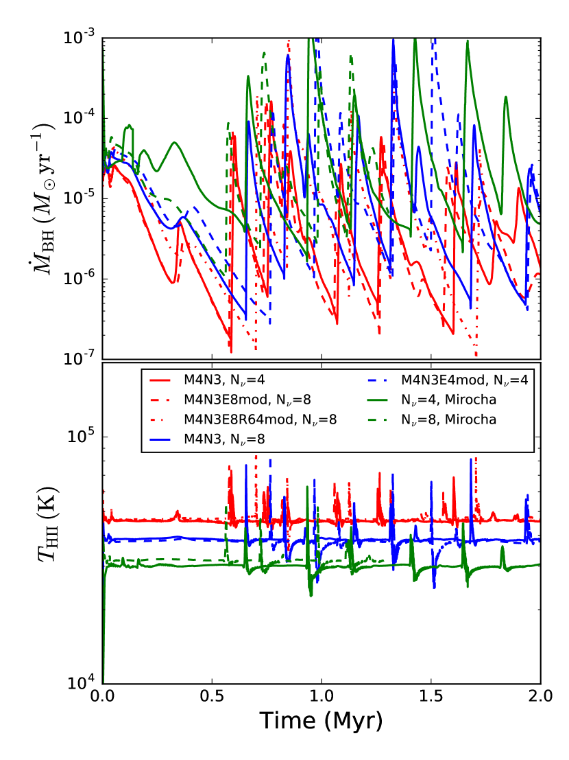
Figure 11.— Accretion rate of BH (top panel) and temperature (bottom panel) of the H ii region for different configurations. The same color indicates the similar results from different setups. For example, red solid line shows the model with $N_{\nu}=4$ with the equally spaced energy bins while red dashed line shows the model with $N_{\nu}=8$ with the modified SED. Both show a similar temperature and accretion rate evolution. The green lines show the results for SED calculated using the method in Mirocha et al. (2012) for $N_{\nu}=4$ (solid) and 8 (dashed).

Table 3Optimized SEDs for $\alpha=1.5$ Power-law BH radiation using Mirocha et al. (2012)

$n_{\nu}$	$N_{\nu}=1$	$N_{\nu}=2$	$N_{\nu}=4$	$N_{\nu}=8$
1	(16.88, 0.995)	(18.47, 0.505)	(18.50, 0.255)	(18.49, 0.105)
2	…	(26.58, 0.505)	(86.90, 0.255)	(45.94, 0.075)
3	…	…	(136.97, 0.055)	(66.11, 0.055)
4	…	…	(236.47, 0.055)	(114.15, 0.075)
5	…	…	…	(125.02, 0.055)
6	…	…	…	(587.44, 0.045)
7	…	…	…	(704.72, 0.055)
8	…	…	…	(6858.18, 0.045)

Figure 10 shows the SED bin energies in log space chosen for different number of energy bins: $N_{\nu}=$ 1 (blue symbol), 2 (green), 4 (red), and 8 (cyan). With increasing $N_{\nu}$, the distribution occupies the energy space more evenly. If the SEDs are chosen in such way that the energy under the curve is preserved, then the lowest energy point shifts toward lower energy values with increasing $N_{\nu}$. Such SEDs have a higher fraction of the ionizing UV photons in proportion to the higher energy ones. The number of the readily absorbed, lower energy UV photons is on the other hand a primary factor determining the temperature profile and size of the H ii region, as described above. Thus, considering the energy under the SED curve is a necessary but not sufficient condition if the goal is to obtain consistent results of photo-ionization calculations. The number of ionizing photons assigned to the first SED bin is also of importance. In order to achieve both conditions, we first construct SEDs according to the “energy under the curve” requirement and modify them, so that the “number of photons in the first SED bin” condition is satisfied.

An example is shown in Figure 10 where squares mark the modified SED energy distribution for $N_{\nu}=8$ which is intended to match the properties of the $N_{\nu}=4$ case for the first energy bin and the total number of ionizing photons. For the first bin of $N_{\nu}=8$ we increase the energy from 21.5 eV to 28.4 eV and also increase the energy fraction from $L_{1}=0.4318$ to $L_{1}^{\prime}=0.4318\times(28.4\,{\rm eV}/21.5\,{\rm eV})=0.5704$ which is adopted in Table 2. The extension to an even larger numbers of SED energy bins $N_{\nu}\gtrsim 16$ should be modeled carefully since more than 2 energy bins are allotted in this case for $E<\langle E\rangle$.

Figure 11 illustrates the results of simulations with different SED configurations. The SED configurations with $N_{\nu}=4$ (red solid) and 8 (blue solid), in which only energy under the curve criterion was considered, clearly exhibit different temperature of the ionized region: $T_{\rm HII}\sim 4.5\times 10^{4}$ K and $4\times 10^{4}$ K, respectively. As a consequence, the accretion rate is higher for $N_{\nu}=8$ case since for the Bondi accretion rate $\dot{M}_{\rm BH}\propto T_{\rm HII}^{-3/2}$.

In the next step, the SED with $N_{\nu}=8$ is modified in such way that its first energy bin has an equal energy and number of UV photons as $N_{\nu}=4$ model (M4N3E8mod, red dashed line). The two runs exhibit indistinguishable temperature evolution in the H ii region and nearly the same (albeit not identical) evolution in the accretion rate. This demonstrates that our approach to modeling the SEDs will give consistent results regardless of the exact numerical configuration of the SED. As an additional test of our method, we also change the first bin for $N_{\nu}=4$ (blue dashed) to mirror the energy but not the number of photons in the first bin of unmodified SED with $N_{\nu}=8$ (M4N3, blue solid). As a result, the temperature evolution in the H ii region is indistinguishable in the two models but the evolution of the accretion rate differs noticeably between $N_{\nu}=8$ (blue solid) and $N_{\nu}=4$ with modification (blue dashed).

We also investigate the effects of numerical resolution coupled with the physics of photo-ionization in a run with a modified SED. M4N3E8R64mod (red dot-dashed) shows the highest resolution test with a $64^{3}$ top grid and 3 levels of refinement. Note that in this run the first burst of accretion is slightly delayed by $\sim$ 0.1 Myr compared to M4N3, however the following sequence of oscillations shows consistent results in terms of the accretion rate and the mean period of oscillation.

Finally, we also test the SEDs for the source with a discretized energy spectrum, which are optimized to recover analytic solutions for the size and thermal structure of H ii region using the method by Mirocha et al. (2012). The SEDs based on this method are listed in Table 3 and shown as triangles in Figure 10. Note that with increasing $N_{\nu}$, the energy of the first bin is fixed at $E\sim 18.5\,$eV which is similar to our strategy for selecting the first energy bin. Green solid ($N_{\nu}=4$) and dashed ($N_{\nu}=8$) lines show the results for this SED configuration. The temperature of H ii region is $T_{\rm HII}\sim 30,000\,$K which is lower than other simulations, and can be understood as a consequence of assigning lower energy to the first SED bin.

References

- Abel et al. (1997) Abel, T., Anninos, P., Zhang, Y., & Norman, M. L. 1997, New A, 2, 181
- Abel et al. (2000) Abel, T., Bryan, G. L., & Norman, M. L. 2000, ApJ, 540, 39
- Abel & Wandelt (2002) Abel, T., & Wandelt, B. D. 2002, MNRAS, 330, L53
- Alvarez et al. (2009) Alvarez, M. A., Wise, J. H., & Abel, T. 2009, ApJ, 701, L133
- Anninos et al. (1997) Anninos, P., Zhang, Y., Abel, T., & Norman, M. L. 1997, New A, 2, 209
- Begelman (1979) Begelman, M. C. 1979, MNRAS, 187, 237
- Begelman et al. (2006) Begelman, M. C., Volonteri, M., & Rees, M. J. 2006, MNRAS, 370, 289
- Blondin & Shaw (2007) Blondin, J. M., & Shaw, S. 2007, ApJ, 656, 366
- Bondi (1952) Bondi, H. 1952, MNRAS, 112, 195
- Bromm et al. (1999) Bromm, V., Coppi, P. S., & Larson, R. B. 1999, ApJ, 527, L5
- Bryan et al. (2014) Bryan, G. L., Norman, M. L., O’Shea, B. W., et al. 2014, ApJS, 211, 19
- Cabral & Leedom (1993) Cabral, B., & Leedom, L. C. 1993, in Proceedings of the 20th Annual Conference on Computer Graphics and Interactive Techniques, SIGGRAPH ’93 (New York, NY, USA: ACM), 263–270. http://doi.acm.org/10.1145/166117.166151
- Carr et al. (1984) Carr, B. J., Bond, J. R., & Arnett, W. D. 1984, ApJ, 277, 445
- Choi et al. (2013) Choi, J.-H., Shlosman, I., & Begelman, M. C. 2013, ApJ, 774, 149
- Davies et al. (2011) Davies, M. B., Miller, M. C., & Bellovary, J. M. 2011, ApJ, 740, L42
- Devecchi & Volonteri (2009) Devecchi, B., & Volonteri, M. 2009, ApJ, 694, 302
- Fan et al. (2001) Fan, X., Narayanan, V. K., Lupton, R. H., et al. 2001, AJ, 122, 2833
- Fan et al. (2003) Fan, X., Strauss, M. A., Schneider, D. P., et al. 2003, AJ, 125, 1649
- Fan et al. (2006) Fan, X., Strauss, M. A., Becker, R. H., et al. 2006, AJ, 132, 117
- Fryer et al. (2001) Fryer, C. L., Woosley, S. E., & Heger, A. 2001, ApJ, 550, 372
- Górski et al. (2005) Górski, K. M., Hivon, E., Banday, A. J., et al. 2005, ApJ, 622, 759
- Haehnelt et al. (1998) Haehnelt, M. G., Natarajan, P., & Rees, M. J. 1998, MNRAS, 300, 817
- Inayoshi et al. (2016) Inayoshi, K., Haiman, Z., & Ostriker, J. P. 2016, MNRAS, 459, 3738
- Katz et al. (2015) Katz, H., Sijacki, D., & Haehnelt, M. G. 2015, MNRAS, 451, 2352
- Kim et al. (2011) Kim, J.-h., Wise, J. H., Alvarez, M. A., & Abel, T. 2011, ApJ, 738, 54
- Kolmogorov (1991) Kolmogorov, A. N. 1991, Proceedings of the Royal Society of London Series A, 434, 9
- Lodato & Natarajan (2006) Lodato, G., & Natarajan, P. 2006, MNRAS, 371, 1813
- Madau & Rees (2001) Madau, P., & Rees, M. J. 2001, ApJ, 551, L27
- Milosavljević et al. (2009) Milosavljević, M., Couch, S. M., & Bromm, V. 2009, ApJ, 696, L146
- Mirocha et al. (2012) Mirocha, J., Skory, S., Burns, J. O., & Wise, J. H. 2012, ApJ, 756, 94
- Novak et al. (2011) Novak, G. S., Ostriker, J. P., & Ciotti, L. 2011, ApJ, 737, 26
- Omukai et al. (2008) Omukai, K., Schneider, R., & Haiman, Z. 2008, ApJ, 686, 801
- Pacucci et al. (2015) Pacucci, F., Volonteri, M., & Ferrara, A. 2015, MNRAS, 452, 1922
- Park & Bogdanović (2017) Park, K., & Bogdanović, T. 2017, ApJ, 838, 103
- Park & Ricotti (2011) Park, K., & Ricotti, M. 2011, ApJ, 739, 2
- Park & Ricotti (2012) —. 2012, ApJ, 747, 9
- Park & Ricotti (2013) —. 2013, ApJ, 767, 163
- Park et al. (2014a) Park, K., Ricotti, M., Di Matteo, T., & Reynolds, C. S. 2014a, MNRAS, 437, 2856
- Park et al. (2014b) —. 2014b, MNRAS, 445, 2325
- Park et al. (2016) Park, K., Ricotti, M., Natarajan, P., Bogdanović, T., & Wise, J. H. 2016, ApJ, 818, 184
- Regan et al. (2017) Regan, J., Visbal, E., Wise, J. H., et al. 2017, ArXiv e-prints, arXiv:1703.03805
- Shakura & Sunyaev (1973) Shakura, N. I., & Sunyaev, R. A. 1973, A&A, 24, 337
- Sijacki et al. (2011) Sijacki, D., Springel, V., & Haehnelt, M. G. 2011, MNRAS, 414, 3656
- Souza Lima et al. (2017) Souza Lima, R., Mayer, L., Capelo, P. R., & Bellovary, J. M. 2017, ApJ, 838, 13
- Sugimura et al. (2016) Sugimura, K., Hosokawa, T., Yajima, H., & Omukai, K. 2016, ArXiv e-prints, arXiv:1610.03482
- Turk et al. (2011) Turk, M. J., Smith, B. D., Oishi, J. S., et al. 2011, ApJS, 192, 9
- Volonteri et al. (2003) Volonteri, M., Haardt, F., & Madau, P. 2003, ApJ, 582, 559
- Volonteri & Rees (2005) Volonteri, M., & Rees, M. J. 2005, ApJ, 633, 624
- Willott et al. (2003) Willott, C. J., McLure, R. J., & Jarvis, M. J. 2003, ApJ, 587, L15
- Willott et al. (2010) Willott, C. J., Delorme, P., Reylé, C., et al. 2010, AJ, 139, 906
- Wise & Abel (2011) Wise, J. H., & Abel, T. 2011, MNRAS, 414, 3458
- Wu et al. (2015) Wu, X.-B., Wang, F., Fan, X., et al. 2015, Nature, 518, 512
- Yajima et al. (2017) Yajima, H., Ricotti, M., Park, K., & Sugimura, K. 2017, ArXiv e-prints, arXiv:1704.05567
- Yoo & Miralda-Escudé (2004) Yoo, J., & Miralda-Escudé, J. 2004, ApJ, 614, L25
- Yue et al. (2014) Yue, B., Ferrara, A., Salvaterra, R., Xu, Y., & Chen, X. 2014, MNRAS, 440, 1263