A Note on
Experiments and Software
For Multidimensional Order Statistics

Abstract

In this note we describe experiments on an implementation of two methods proposed in the literature for computing regions that correspond to a notion of order statistics for multidimensional data. Our implementation, which works for any dimension greater than one, is the only that we know of to be publicly available. Experiments run using the software confirm that half-space peeling generally gives better results than directly peeling convex hulls, but at a computational cost.

1 Introduction

For one dimensional data, the definition of order statistics renders their computation mostly a matter of sorting. There is no direct analog for higher dimensions. In this note we describe experiments on an implementation of two methods proposed in the literature for multivariate data and a third method based on multivariate normality that we use as a benchmark. The software is available for download as open source.

Throughout our discussion, assume that we are presented with $n$ data points in dimension $p$, which we refer to as $\mbox{{\boldmath$x$}}_{i}\in\mathbb{R}^{p},\;i=1,\dots,n$. For $p=1$, where there is an obvious order on the data, it will be useful for our discussion to use the parameter $\alpha$ that specifies that we want the data point with the property that $\alpha n$ data points have larger values, which fits well with our application to multivariate data.

The methods we consider share the property that they produce convex regions that contain $(1-\alpha)n$ points. Since we do not want to delve into issues of interpolation, in the sequel we sometimes use the symbol $\hat{\alpha}$ as the realized value of $\alpha$. Of course, if our interest was in $p=1$ we would have implemented interpolation, but in higher dimension many things are not so obvious.

The methods we employ are a special case of a more general family related to notions of data depth that have attracted some theoretical attention (see, e.g., [5, 8, 17]). However, our interest here is strictly computational and we are not primarily interested in the median or in extremal values, but rather in a multivariate version of the concept of order statistics.

Tukey [15] introduced the idea of depth based on convex hulls demarcated by the intersection of half-spaces defined by the data. Eddy [7] provided some probabilistic interpretation and a concise description of an algorithm, which we employ. See [16] for an updated review of this method and its application. To distinguish our implementation of the algorithm, we use the name halfspace. Our implementation, which works for any dimension $p>1$ is the only that we know of to be publicly available.

Eddy used the title “Convex Hull Peeling,” but a more direct use of that name would seem to have been employed by Barnett [3] where convex hulls defined by the data are successively peeled to define data depth. This algorithm was implemented by McDermott and Lin [12] because they note (and we confirm computationally) that computation of half-space intersections is impractical with a serial implementation applied to massive data sets. We refer to our implementation of direct convex hull peeling as direct.

For benchmarking purposes, we implement a third method that we refer to as mahal. This method is based on a multivariate normal model of the data and defines the points for parameter value $\alpha$ as the $(1-\alpha)n$ points whose Mahalanobis distance [11] from the mean of the data are lowest. This method does not share the robustness properties of halfspace (e.g., to the extent that it could provide something like a median, it would always be very close to the mean), but it provides a useful benchmark, particularly for simulated data drawn from a multivariate normal population.

A closely related issue that is not studied here, is the issue of determining the depth of a given point (see, e.g., [1, 4, 6] . That is, given a point, find out in which depth region it lies. This determination does not require enumerating the regions, but in the case of half-space depth, does require finding the relevant half-spaces. An efficient implementation is provided by [14], who describe an implementation of the methods proposed in [10]. They stop short of enumerating the points that form the intersection of half-spaces and then peeling them, but they provide a very efficient method of finding the halfspaces, which enables rapid determination of the depth of a point. The R package depth [9] provides numerous methods for finding depth and enumerates depth regions for $p=2$.

We proceed as follows. The next section provides a description of the algorithms that we tested. In Section 3 we describe some experiments that compare the methods. The final section offers concluding remarks.

2 Algorithm Descriptions

In all three algorithms, the region is defined as a convex hull. The first two algorithms make use of iterative peeling where points on the convex hulls that are identified are removed from the active data; the third does not. Our algorithms are implemented in Python. We use the pyhull module, which is a Python wrapper for the qhull (http://www.qhull.org/) implementation of the Quickhull algorithm [2], to identify points in a convex hull and to produce the intersection of the half-spaces.

2.1 Halfspace Depth Convex Hull Peeling Algorithm

We implemented the halfspace depth convex hull peeling algorithm – halfspace – as described by Eddy [7] with $n$, $p$, and $\alpha$ as inputs, all $n$ points initially classified as active, and the iteration counter $k$ initially set to zero:

Step 0. Find the hyperplanes defined by all combination of $p$ active points. We count the number of points in each of the induced halfspaces (ignoring the points lying directly on the plane.) We then index the hyperplane by the minimum of these two numbers.

Step 1. Generate the intersection of all halfspaces with index $k$. In the first iteration with $k=0$, this is the same as calculating the convex hull $\mathbb{K}_{k}=conv(N_{k}\cup v_{k})$ of all the available points $N_{k}\cup v_{k}$. This is the convex hull of the whole data-set of points, with $v_{0}=\{\}$ and $N_{0}=N$. For subsequent iterations this is the intersection of all halfspaces defined by the hyperplanes with index $k$.

Step 2. If the number of points contained in intersection of halfspaces is less than $(1-\alpha)n$, terminate. If not, remove the points on the convex hull from the active set, increase $k$ by one, and return to Step 1.

Output: When we reach the $1-\alpha$ quantile, we compare the last two hulls with each other and output the hull with $\hat{\alpha}$ closest to $\alpha$

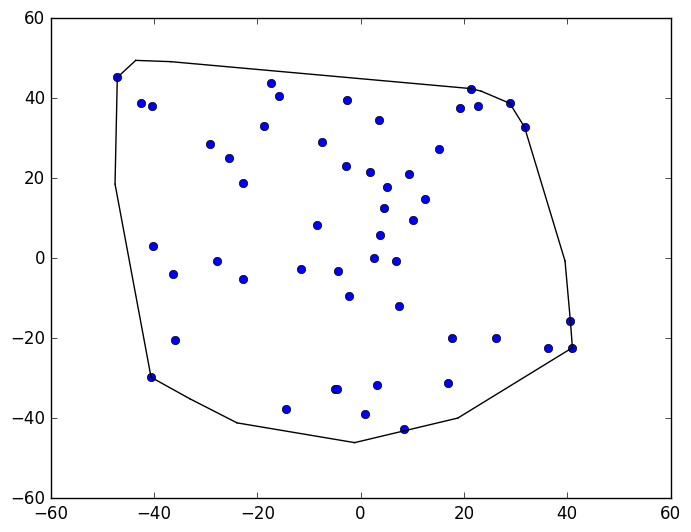
Figure 1: The result of halfspace depth peeling ($\alpha=0.1$) on an example data set.

2.2 Direct Convex Hull Peeling Algorithm

This algorithm – direct – iteratively calculates the convex hull of the active set of points and then removes all the points on the outside faces of the hull. When there are $(1-\alpha)n$ or fewer points in the active data set, the algorithm stops and outputs the points in the hull that contains the number of points closest to $(1-\alpha)n$.

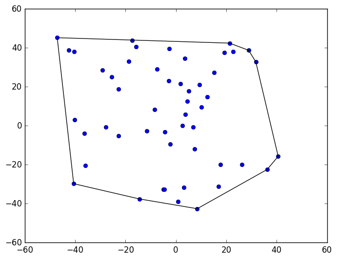
Figure 2: The result of direct convex hull peeling ($\alpha=0.1$) on an example data set.

2.3 Mahalanobis Distance Algorithm

The Mahalanobis distance algorithm – mahal – first uses the mean, $\overline{\mbox{{\boldmath$x$}}}$, and the covariance matrix, $\hat{\Sigma}$ of the full data set to calculate the Mahalanobis distance of each point from the mean. Assuming the data are given as column vectors, a data point $x$ has distance

$$(\mbox{{\boldmath$x$}}-\overline{\mbox{{\boldmath$x$}}})^{T}\Sigma^{-1}(\mbox{{\boldmath$x$}}-\overline{\mbox{{\boldmath$x$}}}).$$

The convex hull of the innermost $\lfloor(1-\alpha)n\rceil$ points provides the desired region, where $\lfloor...\rceil$ denotes rounding to the nearest integer.

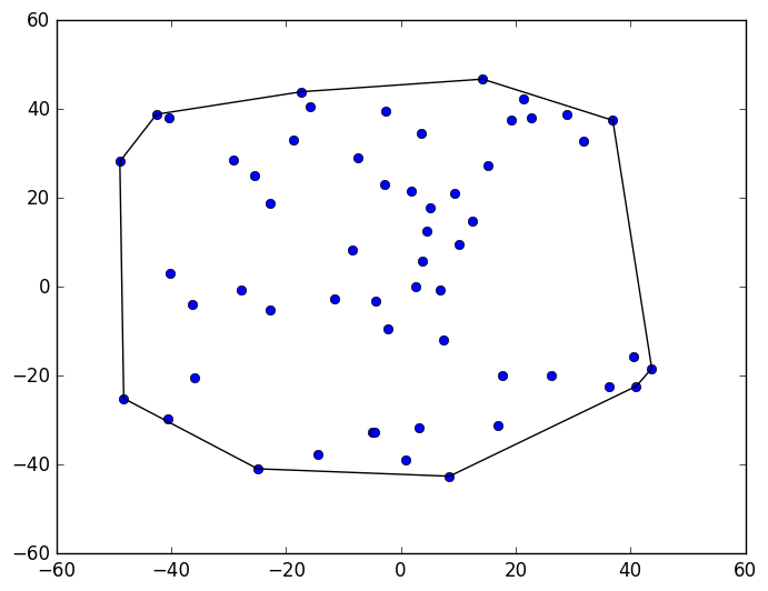
Figure 3: The result of the mahalanobis distance algorithm ($\alpha=0.1$) on an example data set.

3 Computational Experiments

We conduct experiments using $\alpha=0.1,0.5,0.9$. Bear in mind that while for $p=1$, the value of $\alpha=0.5$ would be the median, the corresponding concept of centrality for $p>1$ is the “inner-most peel” which will usually correspond to $\hat{\alpha}<0.1$ for all but small values of $n$; however, our interest is in order statistics not centrality. To measure the quality of shapes that are intended to correspond to order statistics, we consider both the skill and sharpness. For a fixed value of $\alpha$, the sharpness is simply the area (for $p=2$) or volume. We measure the skill using the error. For each replicate we find the hull with a value of $\hat{\alpha}$ close to $\alpha$ for the training data, then we examine test data sets (100 sets in the simulations) and for each test data set we use the difference between the fraction of points inside the hull and $(1-\hat{\alpha})$ as the error. For the practitioners that we work with, skill seems to be the more important of the two measures, but for roughly comparable skill, one would obviously prefer improved sharpness.

3.1 Simulated Data

The simulated data sets we used are generated from multivariate normal distributions with mean zero. For each value of $p$, we generate data sets using one of two covariance matrices and also data sets that have a mixture of data from these two distributions. We use 10 replicates for each value of $n$, $p$, and covariance structure. A replicate consists of a training data set and 100 data sets used to test the skill of the regions found by each method.

We use data two covariance matrices that we refer to as $A$ and $B$ to generate data. A third type of data has $\frac{n}{2}$ points distributed N($\mbox{{\boldmath$0$}},A$) and $\frac{n}{2}$ points distributed N($\mbox{{\boldmath$0$}},B$).

3.1.1 Two-dimensional data

For $p=2$, we use these covariance matrices to simulate data:

$A_{2\times 2}=\begin{bmatrix}1&0.6\\ 0.6&1\end{bmatrix}$. And $B_{2\times 2}=\begin{bmatrix}5&-2\\ -2&5\end{bmatrix}$

In Table 1, we use $\mu$ to refer to the mean error of all 10 replicates and 100 tests for a particular covariance structure. The standard deviation $\sigma$ and the minimum ($min$) and maximum ($max$) of this error over the replicates is also displayed. Note that the direct algorithm has the same values in the experiments that only change the covariance matrix. This is due to the fact that all experiments have the same uniform random numbers as input to make them comparable.

For detailed results, refer to Table 3, Table 4, Table 5 and Table 6. Overall halfspace has the best skill, which it seems to achieve by producing, on average, slightly larger areas (volumes).

3.1.2 Three-dimensional data

For $p=3$, we use these covariance matrices:

$A_{3\times 3}=\begin{bmatrix}1&0.6&0.6\\ 0.6&1&0.6\\ 0.6&0.6&1\end{bmatrix}$ and $B_{3\times 3}=\begin{bmatrix}5&-2&-2\\ -2&5&-2\\ -2&-2&5\end{bmatrix}$.

A summary of results can be seen in Table 2.

The realized $\hat{\alpha}$ for $n=200$ and $p=3$ is much further away from the desired alpha value than any experiment for $p=2$. The realized $\hat{\alpha}$ for $COV=A_{3\times 3}$ with $\alpha=0.1$ for example varies between $0.0$ and $0.2$ for the halfspace depth convex hull peeling algorithm, which is a difference of $0.1$. Even for the $n=100$ case with $COV=A_{2\times 2}$ and $\alpha=0.1$, the halfspace depth convex hull peeling algorithm in the two dimensional case differs only by $0.015$ at most, which confirms that increasing $p$ results in a need for more data points. These results also confirm that the halfspace depth convex hull peeling tends to produce the better skill results.

3.1.3 Runtime

One major drawback of the halfspace depth convex hull peeling algorithm is runtime. Table 7 shows how the different algorithms compare using our serial implementation.

While the overall construction time for the mahalanobis distance and direct convex hull peeling algorithms is about the same for $10$ replicates of any covariance matrix with $n=100$, the halfspace depth convex hull peeling algorithm needed about $3$ times as many seconds in all of the equivalent experiments. Also, the time required for halfspace depth convex hull peeling increases drastically. For $n=500$, the direct convex hull peeling and mahalanobis distance algorithms stay under $20$ seconds run time for all trials. The halfspace depth convex hull peeling meanwhile reaches more than $3000$ seconds ($50$ minutes) in this case. This problem only increases with higher dimensional data. As Eddy notes, this requires O($n^{p+1}$) time, which we see can be significant for our implementation.

The most time consuming part is the creation of all halfspaces and checking how many points are on either side. It would be trivial to parallelize this; however, it would be not so trivial to parallelize finding the intersection, which would eventually become the computational bottleneck.

4 Conclusions

We have described experiments on an implementation of methods proposed in the literature for computing regions that correspond to a notion of order statistics for multidimensional data. The software is publicly available on github under the name morderstats to support use in practice or additional experiments.

Experiments that we report on here confirm that half-space peeling generally gives better results than directly peeling convex hulls, but at a computational cost. One potential avenue for further research is the use of faster methods that could be used to find the planes (see, e.g., [14]) or one could parallelize the method we use. Then computing the intersections would become the bottleneck and a potential topic for further research.

Our work was motivated by wind power prediction intervals [13] where order statistics offer the advantage that they are easy to explain to all stakeholders. They are also useful as a benchmark against which to compare model-based methods. We are now working to simultaneously consider adjacent hours and multiple sources of renewable energy. These applications highlight the need for ongoing research in computational methods for multidimensional order statistics.

References

Appendix A Tables

$\overset{\sigma}{\mu}$			Mahal			Direct			Halfspace
[min, max]	$\alpha=$	0.9	0.5	0.1	0.9	0.5	0.1	0.9	0.5	0.1
	$n=100$	$\overset{.0272}{\underset{[.000,.100]}{.0557}}$	$\overset{.0668}{\underset{[.000,.290]}{.1084}}$	$\overset{.0520}{\underset{[.000,.280]}{.0939}}$	$\overset{.0252}{\underset{[.000,.130]}{.0589}}$	$\overset{.0645}{\underset{[.000,.300]}{.1010}}$	$\overset{.0506}{\underset{[.000,.250]}{.0918}}$	$\overset{.0231}{\underset{[.000,.120]}{.0286}}$	$\overset{.0504}{\underset{[.000,.230]}{.0650}}$	$\overset{.0461}{\underset{[.000,.230]}{.0566}}$
3-11
$COV=A$	$n=200$	$\overset{.0202}{\underset{[.000,.095]}{.0406}}$	$\overset{.0386}{\underset{[.000,.185]}{.0582}}$	$\overset{.0337}{\underset{[.000,.175]}{.0609}}$	$\overset{.0201}{\underset{[.000,.090]}{.0357}}$	$\overset{.0410}{\underset{[.000,.195]}{.0660}}$	$\overset{.0311}{\underset{[.000,.165]}{.0637}}$	$\overset{.0202}{\underset{[.000,.155]}{.0214}}$	$\overset{.0287}{\underset{[.000,.145]}{.0277}}$	$\overset{.0245}{\underset{[.000,.125]}{.0334}}$
3-11
	$n=500$	$\overset{.0144}{\underset{[.000,.070]}{.0248}}$	$\overset{.0225}{\underset{[.000,.114]}{.0296}}$	$\overset{.0160}{\underset{[.000,.082]}{.0259}}$	$\overset{.0142}{\underset{[.000,.066]}{.0214}}$	$\overset{.0242}{\underset{[.000,.126]}{.0387}}$	$\overset{.0182}{\underset{[.000,.098]}{.0322}}$	$\overset{.0115}{\underset{[.000,.054]}{.0119}}$	$\overset{.0183}{\underset{[.000,.092]}{.0207}}$	$\overset{.0123}{\underset{[.000,.068]}{.0123}}$
	$n=100$	$\overset{.0265}{\underset{[.000,.100]}{.0563}}$	$\overset{.0716}{\underset{[.000,.320]}{.1200}}$	$\overset{.0552}{\underset{[.000,.280]}{.0989}}$	$\overset{.0252}{\underset{[.000,.130]}{.0589}}$	$\overset{.0645}{\underset{[.000,.300]}{.1010}}$	$\overset{.0506}{\underset{[.000,.250]}{.0918}}$	$\overset{.0239}{\underset{[.000,.120]}{.0300}}$	$\overset{.0512}{\underset{[.000,.230]}{.0650}}$	$\overset{.0432}{\underset{[.000,.210]}{.0557}}$
3-11
$COV=B$	$n=200$	$\overset{.0198}{\underset{[.000,.095]}{.0406}}$	$\overset{.0388}{\underset{[.000,.205]}{.0716}}$	$\overset{.0353}{\underset{[.000,.190]}{.0680}}$	$\overset{.0201}{\underset{[.000,.090]}{.0357}}$	$\overset{.0410}{\underset{[.000,.195]}{.0660}}$	$\overset{.0311}{\underset{[.000,.165]}{.0637}}$	$\overset{.0200}{\underset{[.000,.155]}{.0208}}$	$\overset{.0295}{\underset{[.000,.145]}{.0306}}$	$\overset{.0241}{\underset{[.000,.125]}{.0315}}$
3-11
	$n=500$	$\overset{.0142}{\underset{[.000,.070]}{.0252}}$	$\overset{.0236}{\underset{[.000,.120]}{.0370}}$	$\overset{.0174}{\underset{[.000,.098]}{.0298}}$	$\overset{.0142}{\underset{[.000,.066]}{.0214}}$	$\overset{.0242}{\underset{[.000,.126]}{.0387}}$	$\overset{.0182}{\underset{[.000,.098]}{.0322}}$	$\overset{.0115}{\underset{[.000,.054]}{.0119}}$	$\overset{.0180}{\underset{[.000,.092]}{.0197}}$	$\overset{.0133}{\underset{[.000,.072]}{.0136}}$
$COV=A$	$n=100$	$\overset{.0244}{\underset{[.000,.100]}{.0575}}$	$\overset{.0583}{\underset{[.000,.260]}{.1006}}$	$\overset{.0531}{\underset{[.000,.310]}{.0975}}$	$\overset{.0262}{\underset{[.000,.120]}{.0581}}$	$\overset{.0608}{\underset{[.000,.270]}{.0939}}$	$\overset{.0550}{\underset{[.000,.280]}{.1063}}$	$\overset{.0233}{\underset{[.000,.130]}{.0280}}$	$\overset{.0461}{\underset{[.000,.220]}{.0684}}$	$\overset{.0479}{\underset{[.000,.250]}{.0655}}$
3-11
and	$n=200$	$\overset{.0200}{\underset{[.000,.090]}{.0397}}$	$\overset{.0387}{\underset{[.000,.205]}{.0679}}$	$\overset{.0285}{\underset{[.000,.140]}{.0538}}$	$\overset{.0227}{\underset{[.000,.100]}{.0420}}$	$\overset{.0364}{\underset{[.000,.180]}{.0582}}$	$\overset{.0269}{\underset{[.000,.140]}{.0588}}$	$\overset{.0184}{\underset{[.000,.100]}{.0251}}$	$\overset{.0243}{\underset{[.000,.135]}{.0231}}$	$\overset{.0212}{\underset{[.000,.110]}{.0310}}$
3-11
$COV=B$	$n=500$	$\overset{.0142}{\underset{[.000,.066]}{.0191}}$	$\overset{.0246}{\underset{[.000,.120]}{.0400}}$	$\overset{.0175}{\underset{[.000,.084]}{.0288}}$	$\overset{.0132}{\underset{[.000,.062]}{.0198}}$	$\overset{.0234}{\underset{[.000,.118]}{.0398}}$	$\overset{.0175}{\underset{[.000,.082]}{.0316}}$	$\overset{.0125}{\underset{[.000,.070]}{.0130}}$	$\overset{.0167}{\underset{[.000,.088]}{.0196}}$	$\overset{.0121}{\underset{[.000,.058]}{.0114}}$

Table 1: Results of experiments with 10 replicates and 100 test data sets for each in dimension $p=2$. The table shows the mean $\mu$ and standard deviation $\sigma$ for the error for all replicates. Each replicate involves generation of a data set of $n$ points and calculation the hull according to $\alpha$ for each algorithm. Each iteration within each replicate then generates $n$ new points with the same covariance structure as the original data set had and counts how many points are inside the generated hull. The mean of the difference between all these numbers and each realized alpha, $\hat{alpha}$, then becomes $\mu$, which is the value in the middle of each cell. $\sigma$ is the standard deviation of all these errors and displayed above the $\mu$ value. The minimum error and maximum error are displayed in the form of $[min,max]$ below the $\mu$ value.

$\overset{\sigma}{\mu}$			Mahal			Direct			Halfspace
[min, max]	$\alpha=$	0.9	0.5	0.1	0.9	0.5	0.1	0.9	0.5	0.1
$COV=A$	$n=200$	$\overset{.0133}{\underset{[.020,.100]}{.0694}}$	$\overset{.0474}{\underset{[.000,.260]}{.1324}}$	$\overset{.0414}{\underset{[.050,.270]}{.1602}}$	$\overset{.0207}{\underset{[.010,.125]}{.0734}}$	$\overset{.0421}{\underset{[.035,.310]}{.1749}}$	$\overset{.0406}{\underset{[.065,.325]}{.1801}}$	$\overset{.0282}{\underset{[.000,.150]}{.0368}}$	$\overset{.0581}{\underset{[.000,.250]}{.0942}}$	$\overset{.0505}{\underset{[.000,.240]}{.1261}}$
$COV=B$	$n=200$	$\overset{.0153}{\underset{[.020,.100]}{.0695}}$	$\overset{.0463}{\underset{[.000,.280]}{.1458}}$	$\overset{.0398}{\underset{[.040,.285]}{.1669}}$	$\overset{.0207}{\underset{[.010,.125]}{.0734}}$	$\overset{.0421}{\underset{[.035,.310]}{.1749}}$	$\overset{.0406}{\underset{[.065,.325]}{.1801}}$	$\overset{.0208}{\underset{[.000,.125]}{.0206}}$	$\overset{.0414}{\underset{[.000,.200]}{.0505}}$	$\overset{.0574}{\underset{[.000,.240]}{.0980}}$
$COX=A$ and $COV=B$	$n=200$	$\overset{.0162}{\underset{[.000,.100]}{.0669}}$	$\overset{.0365}{\underset{[.020,.245]}{.1361}}$	$\overset{.0337}{\underset{[.030,.250]}{.1351}}$	$\overset{.0177}{\underset{[.005,.115]}{.0651}}$	$\overset{.0369}{\underset{[.020,.230]}{.1251}}$	$\overset{.0360}{\underset{[.040,.255]}{.1321}}$	$\overset{.0198}{\underset{[.000,.105]}{.0211}}$	$\overset{.1255}{\underset{[.000,.505]}{.0848}}$	$\overset{.0374}{\underset{[.000,.160]}{.0462}}$

Table 2: Results of experiments with $10$ replicates in dimension $p=3$. The table shows the mean $\mu$ and standard deviation $\sigma$ for the error for all replicates. Each replicate involves generation of a data set of $n$ points and calculation of the hull according to $\alpha$ for each algorithm. Each of the 100 test data sets within each replicate then generates $n$ new points with the same covariance matrix the original data set had and counts how many points are inside the generated hull. The mean of the difference between all these numbers and each realized alpha then becomes $\mu$, which is the value in the middle of each cell. $\sigma$ is the standard deviation of all these errors and displayed above the $\mu$ value. The minimum error and maximum error are displayed in the form of $[min,max]$ below the $\mu$ value.

	$n=100$		Mahal			Direct			Halfspace
	$p=2$	0.9	0.5	0.1	0.9	0.5	0.1	0.9	0.5	0.1
	realized alpha ($\mu$)	0.900	0.500	0.100	0.899	0.509	0.083	0.904	0.504	0.090
	realized alpha ($\sigma$)	0.000	0.000	0.000	0.0166	0.034	0.013	0.007	0.008	0.016
	too many points ($\mu$)	0.080	0.077	0.019	0.029	0.084	0.026	0.369	0.319	0.122
$COV=A$	too many points ($\sigma$)	0.133	0.129	0.035	0.045	0.156	0.048	0.339	0.357	0.148
	too few points ($\mu$)	0.920	0.905	0.967	0.970	0.897	0.957	0.631	0.640	0.819
	too few points ($\sigma$)	0.133	0.148	0.053	0.044	0.172	0.085	0.339	0.365	0.208
	volume ($\mu$)	0.245	3.097	9.150	0.225	2.571	9.360	0.447	3.264	10.213
	volume ($\sigma$)	0.141	0.647	1.073	0.091	0.555	1.344	0.187	0.779	1.526
	realized alpha ($\mu$)	0.900	0.500	0.100	0.899	0.509	0.083	0.902	0.506	0.091
	realized alpha ($\sigma$)	0.000	0.000	0.000	0.017	0.034	0.013	0.004	0.010	0.017
	too many points ($\mu$)	0.080	0.062	0.017	0.029	0.084	0.026	0.369	0.330	0.092
$COV=B$	too many points ($\sigma$)	0.166	0.129	0.030	0.045	0.156	0.048	0.340	0.356	0.096
	too few points ($\mu$)	0.920	0.910	0.970	0.970	0.897	0.957	0.631	0.632	0.855
	too few points ($\sigma$)	0.166	0.172	0.049	0.044	0.172	0.085	0.340	0.364	0.137
	volume ($\mu$)	1.349	15.641	50.953	1.291	14.728	53.616	2.591	18.698	58.502
	volume ($\sigma$)	0.787	3.716	7.267	0.522	3.182	7.701	1.065	4.461	8.739
	realized alpha ($\mu$)	0.900	0.500	0.100	0.894	0.510	0.084	0.903	0.500	0.095
	realized alpha ($\sigma$)	0.000	0.000	0.000	0.018	0.038	0.007	0.008	0.012	0.012
	too many points ($\mu$)	0.059	0.082	0.026	0.043	0.128	0.030	0.367	0.280	0.147
$COV=A,B$	too many points ($\sigma$)	0.166	0.156	0.075	0.116	0.236	0.071	0.324	0.367	0.267
	too few points ($\mu$)	0.941	0.893	0.957	0.952	0.866	0.954	0.633	0.674	0.812
	too few points ($\sigma$)	0.166	0.197	0.109	0.115	0.235	0.103	0.324	0.385	0.306
	volume ($\mu$)	0.432	5.700	32.295	0.462	5.882	35.002	0.828	7.990	40.587
	volume ($\sigma$)	0.196	1.257	7.993	0.239	0.978	9.121	0.339	2.085	10.329

Table 3: Results of experiments with 10 replicates of 100 test data sets each in dimension $p=2$ for $n=100$. The data shows the average realized alpha, $\hat{\alpha}$, over all replicates and all data sets, as well as the average percentage of times generated test data has too many (or too few) points in the generated hull. Averages as labelled $\mu$ and the corresponding standard devations $\sigma$.

	$n=200$		Mahal			Direct			Halfspace
	$p=2$	0.9	0.5	0.1	0.9	0.5	0.1	0.9	0.5	0.1
	realized alpha ($\mu$)	0.900	0.500	0.100	0.901	0.503	0.105	0.901	0.505	0.106
	realized alpha ($\sigma$)	0.000	0.000	0.000	0.013	0.022	0.013	0.002	0.005	0.010
	too many points ($\mu$)	0.057	0.063	0.032	0.081	0.089	0.025	0.435	0.363	0.114
$COV=A$	too many points ($\sigma$)	0.096	0.068	0.060	0.126	0.169	0.065	0.345	0.288	0.139
	too few points ($\mu$)	0.943	0.917	0.954	0.917	0.898	0.967	0.565	0.583	0.851
	too few points ($\sigma$)	0.096	0.080	0.068	0.125	0.189	0.084	0.345	0.289	0.156
	volume ($\mu$)	0.326	3.678	10.842	0.339	2.895	9.162	0.515	3.365	10.239
	volume ($\sigma$)	0.081	0.400	1.142	0.108	0.446	0.668	0.152	0.344	0.867
	realized alpha ($\mu$)	0.900	0.500	0.100	0.901	0.503	0.105	0.901	0.502	0.106
	realized alpha ($\sigma$)	0.000	0.000	0.000	0.013	0.022	0.013	0.002	0.007	0.010
	too many points ($\mu$)	0.034	0.034	0.025	0.081	0.089	0.025	0.430	0.333	0.132
$COV=B$	too many points ($\sigma$)	0.035	0.034	0.051	0.126	0.169	0.065	0.340	0.296	0.165
	too few points ($\mu$)	0.966	0.958	0.965	0.917	0.898	0.967	0.570	0.623	0.828
	too few points ($\sigma$)	0.035	0.043	0.062	0.125	0.189	0.084	0.340	0.299	0.197
	volume ($\mu$)	1.816	17.784	59.061	1.939	16.584	52.483	2.933	19.221	59.208
	volume ($\sigma$)	0.377	1.494	6.116	0.620	2.558	3.825	0.855	1.961	4.711
	realized alpha ($\mu$)	0.900	0.500	0.100	0.896	0.494	0.100	0.902	0.502	0.103
	realized alpha ($\sigma$)	0.000	0.000	0.000	0.015	0.018	0.008	0.003	0.006	0.009
	too many points ($\mu$)	0.080	0.034	0.050	0.096	0.066	0.021	0.343	0.370	0.149
$COV=A,B$	too many points ($\sigma$)	0.155	0.046	0.118	0.200	0.098	0.043	0.372	0.281	0.249
	too few points ($\mu$)	0.920	0.949	0.937	0.904	0.914	0.972	0.657	0.593	0.811
	too few points ($\sigma$)	0.155	0.069	0.138	0.200	0.118	0.061	0.372	0.290	0.257
	volume ($\mu$)	0.557	6.173	37.733	0.584	6.879	37.073	0.831	8.152	42.935
	volume ($\sigma$)	0.172	0.751	4.970	0.168	0.896	3.130	0.263	0.843	5.534

Table 4: Results of experiments with ten replicates of 100 test data sets each in dimension $p=2$ for $n=200$. The data shows the average realized alpha over all replicates and all data sets, as well as the average percentage of times generated test data has too many (or too few) points in the generated hull. Averages as labelled $\mu$ and the corresponding standard devations $\sigma$.

	$n=500$		Mahal			Direct			Halfspace
	$p=2$	0.9	0.5	0.1	0.9	0.5	0.1	0.9	0.5	0.1
	realized alpha ($\mu$)	0.900	0.500	0.100	0.894	0.501	0.104	0.901	0.501	0.102
	realized alpha ($\sigma$)	0.000	0.000	0.000	0.004	0.013	0.012	0.001	0.002	0.003
	too many points ($\mu$)	0.164	0.114	0.086	0.120	0.090	0.027	0.511	0.307	0.285
$COV=A$	too many points ($\sigma$)	0.302	0.090	0.129	0.183	0.151	0.028	0.321	0.297	0.245
	too few points ($\mu$)	0.836	0.859	0.902	0.880	0.898	0.965	0.489	0.667	0.675
	too few points ($\sigma$)	0.302	0.098	0.143	0.183	0.169	0.034	0.321	0.299	0.260
	volume ($\mu$)	0.443	4.242	12.669	0.453	3.122	10.148	0.520	3.373	11.178
	volume ($\sigma$)	0.115	0.225	0.917	0.072	0.192	0.639	0.084	0.220	0.503
	realized alpha ($\mu$)	0.900	0.500	0.100	0.894	0.501	0.104	0.901	0.500	0.102
	realized alpha ($\sigma$)	0.000	0.000	0.000	0.004	0.013	0.012	0.001	0.003	0.004
	too many points ($\mu$)	0.204	0.102	0.045	0.120	0.090	0.027	0.495	0.312	0.262
$COV=B$	too many points ($\sigma$)	0.348	0.172	0.070	0.183	0.151	0.028	0.315	0.282	0.242
	too few points ($\mu$)	0.796	0.890	0.938	0.880	0.898	0.965	0.505	0.662	0.699
	too few points ($\sigma$)	0.348	0.176	0.096	0.183	0.169	0.034	0.315	0.291	0.266
	volume ($\mu$)	2.545	20.121	68.944	2.592	17.882	58.129	2.978	19.350	63.699
	volume ($\sigma$)	0.732	1.430	5.305	0.412	1.098	3.662	0.484	1.267	3.212
	realized alpha ($\mu$)	0.900	0.500	0.100	0.904	0.501	0.102	0.900	0.501	0.101
	realized alpha ($\sigma$)	0.000	0.000	0.000	0.007	0.009	0.009	0.002	0.002	0.004
	too many points ($\mu$)	0.148	0.087	0.047	0.220	0.057	0.032	0.545	0.284	0.301
$COV=A,B$	too many points ($\sigma$)	0.173	0.171	0.058	0.304	0.103	0.049	0.340	0.297	0.241
	too few points ($\mu$)	0.852	0.900	0.936	0.780	0.928	0.961	0.455	0.686	0.656
	too few points ($\sigma$)	0.173	0.197	0.079	0.304	0.120	0.059	0.340	0.306	0.262
	volume ($\mu$)	0.762	6.826	43.891	0.756	7.077	41.022	0.985	7.996	46.339
	volume ($\sigma$)	0.125	0.683	3.497	0.154	0.664	3.874	0.168	0.670	3.057

Table 5: Results of experiments with ten replicates, dimension $p=2$ for $n=500$. The data shows the average realized alpha over all replicates and all data sets, and the average percentage of times generated test data has too many (or too few) points in the generated hull. Averages as labelled $\mu$ and the corresponding standard devations $\sigma$.

	$n=200$		Mahal			Direct			Halfspace
	$p=3$	0.9	0.5	0.1	0.9	0.5	0.1	0.9	0.5	0.1
	realized alpha ($\mu$)	0.900	0.500	0.100	0.887	0.484	0.128	0.903	0.522	0.029
	realized alpha ($\sigma$)	0.000	0.000	0.000	0.029	0.045	0.015	0.011	0.038	0.062
	too many points ($\mu$)	0.000	0.002	0.000	0.000	0.000	0.000	0.665	0.920	0.010
$COV=A$	too many points ($\sigma$)	0.000	0.004	0.000	0.000	0.000	0.000	0.386	0.116	0.032
	too few points ($\mu$)	1.000	0.996	1.000	1.000	1.000	1.000	0.335	0.061	0.986
	too few points ($\sigma$)	0.000	0.007	0.000	0.000	0.000	0.000	0.386	0.096	0.041
	volume ($\mu$)	0.354	8.042	23.520	0.421	5.303	18.115	1.375	11.950	33.960
	volume ($\sigma$)	0.064	1.324	2.427	0.211	1.107	2.241	0.438	1.728	5.974
	realized alpha ($\mu$)	0.900	0.500	0.100	0.887	0.484	0.128	0.897	0.515	0.081
	realized alpha ($\sigma$)	0.000	0.000	0.000	0.029	0.045	0.015	0.010	0.020	0.086
	too many points ($\mu$)	0.000	0.000	0.000	0.000	0.000	0.000	0.645	0.664	0.055
$COV=B$	too many points ($\sigma$)	0.000	0.000	0.000	0.000	0.000	0.000	0.292	0.352	0.160
	too few points ($\mu$)	1.000	0.999	1.000	1.000	1.000	1.000	0.351	0.308	0.929
	too few points ($\sigma$)	0.000	0.003	0.000	0.000	0.000	0.000	0.295	0.345	0.190
	volume ($\mu$)	4.417	75.264	251.685	4.966	62.567	213.727	15.693	117.871	358.733
	volume ($\sigma$)	1.711	12.566	22.361	2.493	13.066	26.442	3.851	15.147	65.221
	realized alpha ($\mu$)	0.900	0.500	0.100	0.901	0.505	0.110	0.899	0.516	0.116
	realized alpha ($\sigma$)	0.000	0.000	0.000	0.027	0.030	0.016	0.009	0.060	0.065
	too many points ($\mu$)	0.002	0.000	0.000	0.000	0.000	0.000	0.600	0.769	0.096
$COV=A,B$	too many points ($\sigma$)	0.004	0.000	0.000	0.000	0.000	0.000	0.333	0.307	0.096
	too few points ($\mu$)	0.998	1.000	1.000	1.000	1.000	1.000	0.400	0.213	0.870
	too few points ($\sigma$)	0.004	0.000	0.000	0.000	0.000	0.000	0.333	0.296	0.118
	volume ($\mu$)	0.686	15.941	174.555	0.735	20.455	173.824	2.634	71.708	275.968
	volume ($\sigma$)	0.232	2.324	22.007	0.518	5.692	32.283	0.711	50.054	72.006

Table 6: Results of experiments with ten replicates in dimension $p=3$ for $n=200$. The data shows the average realized alpha out of all replicates and all data sets, and the average percentage of times generated test data has too many (or too few) points in the generated hull. Averages as labelled $\mu$ and the corresponding standard devations $\sigma$.

runtime				Mahal			Direct			Halfspace
$p$	$n$	$COV$	0.9	0.5	0.1	0.9	0.5	0.1	0.9	0.5	0.1
		$A$	14.9	14.6	15.1	15.1	14.8	15.6	50.5	42.1	39.8
	$n=100$	$B$	19.4	15.2	15.4	15.2	15.9	15.2	51.9	43.1	39.5
		$A,B$	15.7	14.9	15.0	15.3	15.0	15.5	51.3	42.8	39.0
		$A$	16.6	17.9	17.3	16.8	16.7	16.9	277.8	252.7	244.4
$p=2$	$n=200$	$B$	17.3	16.8	16.8	17.1	17.1	16.5	297.3	255.4	239.4
		$A,B$	17.2	16.5	18.0	16.7	16.6	17.3	315.9	242.8	234.3
		$A$	16.9	16.9	17.2	17.4	16.6	17.1	3585.1	3228.5	3110.8
	$n=500$	$B$	16.8	17.4	17.5	17.0	17.1	17.1	3538.4	3255.9	3065.9
		$A,B$	17.2	17.2	20.7	17.2	16.8	17.0	3509.1	3318.3	3094.6
		$A$	24.0	25.3	23.4	23.2	22.6	23.2	18668.8	17187.6	18271.0
$p=3$	$n=200$	$B$	23.6	22.8	23.2	22.8	22.6	22.5	18233.0	17267.5	18010.7
		$A,B$	25.1	26.2	24.5	22.6	23.8	23.4	18171.9	17233.8	17076.9

Table 7: Total runtime in seconds of the construction time of ten replicates for the experiments summarized in Table 1 and Table 2. These experiments were run on a 64-Bit UNIX system with an $\mbox{Intel}_{\mbox{\textregistered}}$ $\mbox{Core}^{\mbox{\texttrademark}}$ i7 CPU 860 @ 2.80GHz processor.

References

- [1] Greg Aloupis, Carmen Cortés, Francisco Gómez, Michael Soss, and Godfried Toussaint. Lower bounds for computing statistical depth. Comput. Stat. Data Anal., 40(2):223–229, August 2002.
- [2] C. Bradford Barber, David P. Dobkin, and Hannu Huhdanpaa. The quickhull algorithm for convex hulls. ACM Transactions on Mathematical Software, 22(4):469–483, 1996.
- [3] V. Barnett. The ordering of multivariate data. Journal of the Royal Statistical Society, Series A, 139:318––352, 1976.
- [4] David Bremner, Dan Chen, John Iacono, Stefan Langerman, and Pat Morin. Output-sensitive algorithms for tukey depth and related problems. Statistics and Computing, 18(3):259, 2008.
- [5] D. Donoho and M. Gasko. Breakdown properties of location estimates based half-space depth and projected outlyingness. Ann. Statist., 20:1803––1827, 1992.
- [6] R. Dyckerhoff and P. Mozharovskyi. Exact computation of the halfspace depth. Comput. Statist. Data Anal., 98:19––30, 2016.
- [7] W.F. Eddy. Convex hull peeling. In COMPSTAT 1982 5th Symposium held at Toulouse, pages 42–47, 1982.
- [8] John HJ Einmahl, Jun Li, Regina Y Liu, et al. Bridging centrality and extremity: Refining empirical data depth using extreme value statistics. The Annals of Statistics, 43(6):2738–2765, 2015.
- [9] Maxime Genest, Jean-Claude Masse, and Jean-Francois Plante. depth: Nonparametric depth functions for multivariate analysis. https://CRAN.R-project.org/package=depth, 2017.
- [10] Marc Hallin, Davy Paindaveine, and Miroslav Šiman. Multivariate quantiles and multiple-output regression quantiles: From optimization to halfspace depth. Ann. Statist., 38(2):635–669, 04 2010.
- [11] P.C. Mahalanobis. On the generalised distance in statistics. In Proceedings of the National Institute of Sciences of India, volume 2, pages 49–55, 1936.
- [12] James P. McDermott and Dennis K. J. Lin. Quantile contours and multivariate density estimation for massive datasets via sequential convex hull peeling. IIE Transactions, 39(6):581–591, 2007.
- [13] Sabrina Nitsche, César A. Silva-Monroy, Andrea Staid Jean-Paul Watson, Scott Winner, and David L. Woodruff. Improving wind power prediction intervals using vendor-supplied probabilistic forecast information. In IEEE Power and Energy Society General Meeting (PES), pages 1–5. IEEE, 2017.
- [14] Davy Paindaveine and Miroslav Šiman. Computing multiple-output regression quantile regions. Computational Statistics and Data Analysis, 56(4):840 – 853, 2012.
- [15] J. Tukey. Mathematics and the picturing of data. In Proc. 1975 Inter. Cong. Math., Vancouver, Canada, page 523–531. Canad. Math. Congress., 1975.
- [16] G.B. Weller and W.F. Eddy. Multivariate order statistics: Theory and application. Annual Review of Statistics and Its Application, 2(1):237–257, 2015.
- [17] Yijun Zuo and Robert Serfling. General notions of statistical depth function. Ann. Statist., 28(2):461–482, 04 2000.