Two famous results of Einstein derived from the Jarzynski equality

Abstract

The Jarzynski equality (JE) is a remarkable statement relating transient irreversible processes to infinite-time free energy differences. Although twenty years old, the JE remains unfamiliar to many; nevertheless it is a robust and powerful law. We examine two of Einstein’s most simple and well-known discoveries, one classical and one quantum, and show how each of these follows from the JE. Our first example is Einstein’s relation between the drag and diffusion coefficients of a particle in Brownian motion. In this context we encounter a paradox in the macroscopic limit of the JE which is fascinating, but also warns us against using the JE too freely outside of the microscopic domain. Our second example is the equality of Einstein’s $B$ coefficients for absorption and stimulated emission of quanta. Here resonant light does irreversible work on a sample, and the argument differs from Einstein’s equilibrium reasoning using the Planck black-body spectrum. We round out our examples with a brief derivation and discussion of Jarzynski’s remarkable equality.

I Introduction

Suppose a system initially in equilibrium at a temperature $T$ is transiently disturbed, perhaps dramatically, over some limited interval of time. The disturbance will incur some amount of external work $W$, and it may leave the system in some new state.

Since the microscopic state of the system is a matter of probability, the irreversible work done in any particular trial will vary. Furthermore $W$ certainly depends on details of the disturbance, and some or all of it may be dissipated as heat. For these reasons one would expect $W$ to be only loosely connected with the equilibrium eventually reached. The Jarzynski equality (JE) confounds this expectation with the exact average Jarz1997a ; Jarz1997b

$${\langle{e^{-\beta W}}\rangle}\;=\;e^{-\beta\Delta F}$$ (1)

where $\beta=1/{k_{\text{\tiny B}}T}$ and $\Delta F$ is the change in Helmholtz free energy at an infinite time, after the system has found its new equilibrium. It is remarkable that $\Delta F$ is so directly linked to the history of the disturbance. The Jarzynski equality holds both classically and quantum-mechanically, and generalizes to cases where the initial and final temperatures are not equal (Section VI).

Eq (1) is a remarkable statement that invites explanation and application. Over the past two decades the JE, along with its generalization to the “fluctuation theorems” of Crooks, Crooks1998 ; Crooks1999 ; Crooks2000 Evans and Searles EvansSearles2002 and others, have been important in such areas as calculational and experimental molecular dynamics.Hummer2001 ; Bustamante2005 ; Harris2007 ; Jarz2011 On the pedagogical side, however, the JE remains exotic, and absent even from otherwise excellent textbooks on statistical mechanics.Peliti2011 Helpful expositions of (1) have included a very nice application to gas in a piston,LuaGrosberg2005 and interesting applications to systems of springsHijar2010 and to magnetic resonance phenomena.Ribeiro2016 These and other treatments have been valuable and rewarding to work through. Nonetheless, illustrations of the JE have sometimes struck the author as somewhat artificial, or tangential to the mainstream of physics.

Seeking evidence for the centrality and robustness of the JE and fluctuation theorems in areas of physics he currently teaches, the author examined two of Einstein’s widely known discoveries, one classical and one quantum. Both results, while simple, are of deep significance. To the author’s surprise, it became evident that the Jarzynski equality implies each of these results.

The first example to be considered is Einstein’s relation between diffusion and drag coefficients, central to Brownian motion and historically the first fluctuation-dissipation theorem, or FDTLandau ; Reif ; Marconi2008 (different from the fluctuation theorems mentioned above). A connection between FDTs and the Jarzynski equality was previously noted by L. Y. Chen,Chen2008a ; Crooks2009 but our diffusion-drag relation is especially useful not only for its simplicity, but because it illustrates a paradox (Section IV) of a type noted by Jarzynski and others,JarzRare2006 ; LuaGrosberg2005 in the macroscopic limit of the average in Eq (1). Such paradoxes are an important warning against using the JE as freely as one might use, say, the Gibbs distribution.

Our second example is Einstein’s conclusion of the necessity of stimulated emission, and the equality of the coefficients of absorption and stimulated emission. Einstein’s original argument is based on Planck’s black-body spectrum,Eisberg and is a staple of undergraduate courses on modern physics. Stimulated emission is also derived in advanced quantum mechanics as a consequence of the quantum statistics of boson fields such as photons.ZimanAQM We obtain the result from the Jarzynski equality by viewing absorbed and emitted quanta as work done on a thermal system of two-state atoms, whose free energy change is straightforwardly calculated. A surprising feature is that this argument does not explicitly invoke the Bose nature of the quanta.

Derivations of the Jarzynski equality in the literature vary in length and accessibility. In Section VI we provide an adaptation of an efficient quantum-mechanical derivation of the JE and a generalization of it, both due to D. N. Page.Page2012 Finally, in Section VI we mention the importance of time reversal as the underlying basis of the Jarzynski equality.

II Strategy for applying the JE

In each of our examples, our strategy will be to rewrite the average ${\langle{e^{-\beta W}}\rangle}$ on the left side of the JE by using the leading terms of a cumulant expansion, a statistical device useful throughout theoretical physics.Peliti2011 In our case this expansion is

$${\langle{e^{-\beta W}}\rangle} \;=\;e^{-\beta\overline{W}+(\beta^{2}/2)(\overline{W^{2}}-\overline{W}^{2})+\dots}.$$ (2)

The quantity $\overline{W^{2}}-\overline{W}^{2}=\overline{\Delta W^{2}}$ in the exponential is the variance, or mean-squared variation of $W$. Eq (2) is related to the statistical statement ${\langle{e^{X}}\rangle}\geq e^{{\langle{X}\rangle}}$, which when applied to the JE to yields the thermodynamic law $\Delta F\leq W$ as a consequence of the Jarzynski equality.Jarz1997a

Eq (2) can be verified if desired, by expanding $e^{-\beta W}$ in a series, averaging the terms, taking a logarithm and then expanding this again in series.

We make a few additional points. Derivations of the JE like that of Section VI assume a specified time-dependence of the system Hamiltonian $H$, quantum or classical. This is not a strong restriction, however. For example, any classical force $f(t)$ is representable in $H$ by a term $-xf(t)$. Such a classical $f(t)$ is used in our first example below. In the derivation of Section VI we see how work is defined quantum mechanically to arrive at the JE. Our second example below will introduce quantum work consistent with that definition.

The use of a specific temperature in Eq (1) implies contact with a heat bath; one might infer that the JE is a feature of open systems. In fact, the quantum JE derivation in Section VI assumes and requires a closed system. Thus, strictly speaking, Eq (1) is being applied to the system of interest together with its heat reservoir. For a small closed system without a reservoir, irreversible work done on a closed system may in fact leave it at a changed temperature, and this situation is handled by the generalized Jarzynski equality in Section VI.

III Einstein’s diffusion relations from Jarzynski’s equality

Our first and simplest application of the Jarzynski equality is to a particle executing Brownian motion in a viscous medium, a problem considered by Einstein in 1905. We seek to establish Einstein’s relation relating the drag coefficient of the particle and its diffusion constant, both to be defined below.

To apply the JE, we must construct some protocol in which a variable amount of irreversible work will be done on the system. We choose to apply a constant force $f$ to the diffusing particle for a fixed time $\Delta t$. In each episode or trial the displacement $\Delta x$ of the particle, and thus the work done,

$$W=f\Delta x,$$ (3)

is variable. In the JE we average ${\langle{e^{-\beta W}}\rangle}$ over episodes.

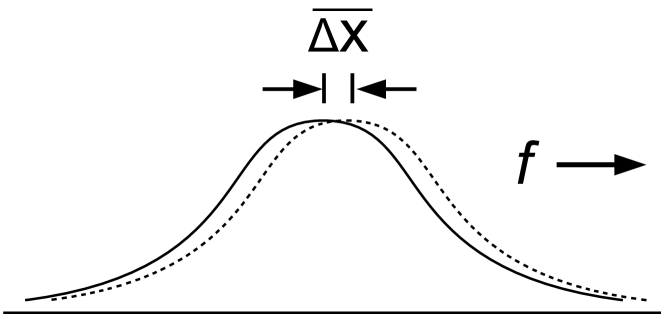
Figure 1: If a small enough force $f$ is applied to a diffusing Brownian particle, the forced displacement $\overline{\Delta x}$ is much smaller than the width $(\Delta x)_{\text{rms}}$ of the diffusional profile, so that $\overline{\Delta x^{2}}$ can be assumed to be that of free diffusion.

With only dissipative work being done there is no free energy change: $\Delta F=0$. Setting $e^{-\beta\Delta F}=1$ in Eq (1) gives us the Jarzynski equality for forcing against pure drag or friction,

$${\langle{e^{-\beta W}}\rangle} \;=\;1.$$ (4)

To apply a cumulant expansion we need $\overline{\Delta W^{2}}$. In the limit of small $f$, the forced displacement will be much smaller than the r.m.s. diffusion (see Figure 1), so we can assume, to zeroth order, a free diffusion. The mean squared displacement of a free diffusion is $\overline{\Delta x^{2}}=2D\Delta t$, defining the diffusion constant $D$. Thus

$$\overline{\Delta W^{2}}\;=\;f^{2}\overline{\Delta x^{2}}\;\approx\;2Df^{2}\Delta t\,.$$ (5)

Now we can apply the cumulant expansion of Eq (2). To lowest order in the force $f$ (and thus in $W$ by Eq (3)) Reviewersuggest

$$e^{-\beta\overline{W}+(\beta^{2}/2)\overline{\Delta W^{2}}}\;\approx\;1,$$ (6)

$$\overline{\Delta W^{2}}\;\approx\;2{k_{\text{\tiny B}}T}\,\overline{W}.$$ (7)

Inserting (5) and $\overline{W}=f\overline{\Delta x}$ from (3), we have

$$2Df^{2}\Delta t\;=\;2{k_{\text{\tiny B}}T}\,f\overline{\Delta x}.$$ (8)

The drag coefficient $\gamma$ is defined by writing the drag force, equal and opposite to our imposed force, as $f=\gamma v=\gamma\overline{\Delta x}/\Delta t$. Using this in (8), we obtain

$$\gamma D\;=\;{k_{\text{\tiny B}}T}.$$ (9)

This is Einstein’s famous relation between drag and diffusion coefficients, i.e. between dissipation and fluctuation. It is central to a variety of applications.Reif ; Nelson Such fluctuation-dissipation theorems or FDTs, which we have found to be a consequence of Jarzynski’s equality, arise not only in particle diffusion but in other phenomena, such as Johnson noise. A treatment of voltage, resistance and current would in that case be essentially identical to what has been done here. A generic identification of first-order expansions of the JE with FDTs (essentially our Eq (7)) has been noted previously by L. Y. Chen.Chen2008a ; Crooks2009 We will not here construct arguments for other FDTs.

IV Macroscopic limit of the JE

Even if the above reasoning is relatively straightforward, the Jarzynski equality in Eq (4) for a pure drag or friction invites a fundamental objection.JTDobjection Pulling a macroscopic object through (say) thick molasses requires a fairly definite amount of work $W$. In repeated trials, $e^{-\beta W}$ ought then to remain close to a value smaller than $1$ in essentially every trial. On the other hand, the JE in Eq (4) strictly requires ${\langle{e^{-\beta W}}\rangle}=1$. How can this be possible?

The resolution of this paradox highlights peculiarities of the average ${\langle{e^{-\beta W}}\rangle}$. In our case of friction or drag, suppose we drag a block across a surface against friction. Molecular motions in the substrate could in principle impart (rather than remove) macroscopic momentum, reversing the force and making $W$ negative—we would have to restrain the block! These negative-$W$ trajectories must exist, as time reversals of trajectories we do observe, but they are suppressed by fantastically small Boltzmann probabilities of order $e^{-\beta|W|}$, that reflect the entropic cost of removing energy from microscopic degrees of freedom. On the other hand, they contribute enormous values $e^{+\beta|W|}$ to the Jarzynski average that compensate for small probabilities. In this way, a macroscopic limit of the average ${\langle{e^{-\beta W}}\rangle}$ will be held to its required value by the contributions of fantastically unlikely scenarios.

Jarzynski has emphasizedJarzRare2006 this dominance of “rare realizations” in ${\langle{e^{-\beta W}}\rangle}$ and the role of time-reversed trajectories, as well as the puzzle of the macroscopic limit for this average in an adiabatic process.JarzPers2007 ; CrooksJarz2007

V Stimulated emission from Jarzynski’s equality

Our second application of the Jarzynski equality is to the phenomenon of stimulated emission. We want to show that any light-absorbing two-state system must also undergo stimulated emission, and that the absorption and emission rates (to be defined) must be equal.

When Einstein considered this problem in 1916, he assumed the light to be in thermal equilibrium (a Planck black-body distribution). To apply the JE, we instead do irreversible work on a “sample” of $N$ two-state subsystems at temperature $T$ (see Figure 2), by applying light to it for a fixed time. The incident light is not thermal; instead its energy $\hbar\omega$ matches the excitation energy of the subsystems.

We will write the work $W$ in terms of the number of absorptions and emissions that occur, in each trial, and as usual evaluate ${\langle{e^{-\beta W}}\rangle}$ with a cumulant expansion, to lowest order in $\beta$ (a high-temperature limit). Next, in $\Delta F$, we will need the entropy change $\Delta S$ of the 2-state systems given the average number of up and down state changes. Finally we will solve the JE in our high-temperature limit for the stimulated emission.

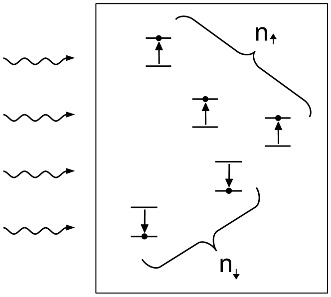
Figure 2: Model system of resonant light with intensity $I$ and fixed duration, illuminating a collection of thermalized two-state subsystems. The subsystems are spatially separated so that their interactions with the light occur independently. During each trial, $n_{\scriptscriptstyle\uparrow}$ absorptions and $n_{\scriptscriptstyle\downarrow}$ induced emissions occur. Spontaneous emission is excluded from consideration by assuming the thermal re-equilibration of states to be fast.

Initially ${{n}}$ of our subsystems are in the upper state and $N-{{n}}$ are in the lower state, a Boltzmann distribution. Under a light of intensity $I$, the work due to $n_{\scriptscriptstyle\uparrow}$ absorptions and $n_{\scriptscriptstyle\downarrow}$ emissions is

$$W\;=\;\hbar\omega({n}_{\scriptscriptstyle\uparrow}{-}{n}_{\scriptscriptstyle\downarrow}).$$ (10)

For our cumulant expansion we will need the variance $\overline{\Delta W^{2}}=\overline{W^{2}}-{\overline{W}}^{2}$. Since $n_{\scriptscriptstyle\uparrow}$ and $n_{\scriptscriptstyle\downarrow}$ are independent, their variances simply add. Also, as random counts, they are Poisson variablesReif for which the variance is equal to the mean. Using these facts we can obtain from (10)

$$\overline{\Delta W^{2}}\;=\;(\hbar\omega)^{2}(\overline{n}_{\scriptscriptstyle\uparrow}+\overline{n}_{\scriptscriptstyle\downarrow}).$$ (11)

Now we invoke the Jarzynski equality, Eq (1). As in our previous example, we apply the cumulant expansion of Eq (2) to ${\langle{e^{-\beta W}}\rangle}$. On the right side of the JE we need the free energy change of the system, $\Delta F=\overline{W}-T\Delta S$, with $\Delta S$ the entropy change due to changes in upper- and lower-state occupation. The JE becomes

$$e^{-\beta\overline{W}+(\beta^{2}/2)\overline{\Delta W^{2}}+\dots}\;=\;e^{-\beta\overline{W}+\Delta S/{k_{\text{\tiny B}}}}.$$ (12)

The term $-\beta\overline{W}$ cancels out. Keeping only leading order in $\beta$, our high-temperature limit, and inserting Eq (11),

$$(\hbar\omega)^{2}(\overline{n}_{\scriptscriptstyle\uparrow}+\overline{n}_{\scriptscriptstyle\downarrow}) \;=\;2({k_{\text{\tiny B}}T})^{2}\Delta S/{k_{\text{\tiny B}}}\,.$$ (13)

This set of $N$ two-state systemsReif is a basic model in introductory statistical mechanics, and its entropy is

$$S \;=\;{k_{\text{\tiny B}}}\ln\frac{N!}{(N{-}{{n}})!\,{{n}}!}$$ (14)

when $n$ are in the upper state. For $\Delta S$ under a change $\overline{\Delta n}=\overline{n}_{\scriptscriptstyle\uparrow}{-}\overline{n}_{\scriptscriptstyle\downarrow}$ we approximate

$$\Delta S \;\approx\;\frac{\partial S}{\partial n}\,(\overline{n}_{\scriptscriptstyle\uparrow}{-}\overline{n}_{\scriptscriptstyle\downarrow}).$$ (15)

ApproximatingReif $\partial(\ln n!)/\partial n\approx\ln n$ to differentiate (14), and using Boltzmann probabilities for the states,

$$\frac{\partial S}{\partial{{n}}} \;\approx\;{k_{\text{\tiny B}}}\ln\frac{N{-}{{n}}}{{{n}}}\;=\;{k_{\text{\tiny B}}}\ln(e^{\beta\hbar\omega})\;=\;\hbar\omega/T.$$ (16)

Inserting this with (15) into Eq (13) gives us

$$\hbar\omega\,(\overline{n}_{\scriptscriptstyle\uparrow}+\overline{n}_{\scriptscriptstyle\downarrow})\;=\;2{k_{\text{\tiny B}}T}\,(\overline{n}_{\scriptscriptstyle\uparrow}{-}\overline{n}_{\scriptscriptstyle\downarrow}).$$ (17)

Finally, the Boltzmann ratio of subsystems in the upper state to those in the lower state is $n/(N{-}n)=\exp(-\hbar\omega/{k_{\text{\tiny B}}T})$. From this, in our high-temperature limit where ${{n}}\approx N/2$, i.e. where $N/2-{{n}}$ is small,

$$\frac{\hbar\omega}{{k_{\text{\tiny B}}T}}\;=\;\ln\frac{N-{{n}}}{{{n}}}\;\approx\;(4/N)\Big{(}\frac{N}{2}-{{n}}\Big{)}.$$ (18)

Following Einstein, the absorption and stimulated emission are proportional to the light intensity and the number in the respective states,

$$\overline{n}_{\scriptscriptstyle\uparrow}=(N{-}{{n}})BI,\quad\overline{n}_{\scriptscriptstyle\downarrow}={{n}}\widetilde{B}I$$ (19)

where $B$ is the coefficient of absorption and $\widetilde{B}$ is Einstein’s postulated coefficient of stimulated emission. Combining the last three equations we get

$$(N{-}2{{n}})[(N{-}{{n}})B+{{n}}\widetilde{B}] \;=\;N[(N{-}{{n}})B-{{n}}\widetilde{B}]$$ (20)

which is easily seen to be solved by

$$\widetilde{B}\;=\;B.$$ (21)

Stimulated emission is found to be necessary, and furthermore we get Einstein’s equality of the $B$ coeffients.

The quanta involved in stimulated emission of course must obey Bose-Einstein statistics, so it is interesting that equivalence of the $B$ coefficients as obtained here does not explicitly invoke the Bose nature of the quanta, involving as it does only the work on, and the free energy of, the collection of two-state systems. By contrast, in Einstein’s original argumentEisberg Bose statistics are introduced by the use of Planck’s black-body spectrum, and in second-quantized field theoryZimanAQM stimulated emission is a specific property of boson fields.

Historically, on the other hand, it has been emphasized by JaynesReviewersuggest ; Jaynes and others that one can reproduce the rules of absorption and stimulated emission by treating the light field classically while retaining the quantum nature of the absorbers, as we have done in a simple way here with our discrete subsystems.

VI A derivation of Jarzynski’s equality

Many derivations of the Jarzynski equality and related fluctuation theorems by Crooks and others are available. Here we rework a particularly efficient quantum argument for the JE by D. N. Page,Page2012 which we follow with some brief commentary. Suppose a system is described by a time-independent Hamiltonian operator $H$. In Gibbs equilibrium the probability of being in an energy eigenstate ${\phi_{i}}$ with energy $E_{i}$ is

$$p_{i}=Z(\beta)^{-1}e^{-\beta E_{i}}$$ (22)

where the partition function is

$$Z(\beta)=\sum_{i}e^{-\beta E_{i}}=e^{-\beta F}$$ (23)

and $F$ is the Helmholtz free energy. Now suppose an external interaction causes $H$ to change over some time interval into a new $H^{\prime}$. The $i$th eigenstate and energy change smoothly into some new ${\phi^{\prime}_{i}}$ and $E^{\prime}_{i}$, but there will also be induced transitions. Denote by $P_{i{\rightarrow}j}$ the probability that a system in state ${\phi_{i}}$ is subsequently found in ${\phi^{\prime}_{j}}$. A specific choice for microscopic work must be madeCrooks2009 and our quantum definition is $E^{\prime}_{j}-E_{i}$, pairwise between states. Then

$${\langle{e^{-\beta(E^{\prime}-E)}}\rangle} =\sum_{i,j}e^{-\beta(E^{\prime}_{j}-E_{i})}p_{i}P_{i{\rightarrow}j}$$ (24)

$$=\sum_{i,j}\big{[}e^{-\beta(E^{\prime}_{j}-E_{i})}\big{]}\big{[}e^{-\beta E_{i}}/Z(\beta)\big{]}P_{i{\rightarrow}j}$$ (25)

$$=\sum_{j}e^{-\beta E^{\prime}_{j}}\big{(}\sum_{i}P_{i{\rightarrow}j}\big{)}/Z(\beta)$$ (26)

$$=Z^{\prime}(\beta)/Z(\beta).$$ (27)

We have used $\sum_{i}P_{i{\rightarrow}j}=1$. With $F$ defined as in (23),

$${\langle{e^{-\beta W}}\rangle}\;=\;Z^{\prime}(\beta)/Z(\beta)\;=\;e^{-\beta(F^{\prime}-F)}$$ (28)

which is the desired equality. The notation $Z^{\prime}$ indicates use of energies $E^{\prime}_{i}$ in this partition function.

The above system is closed. The fact that we keep $\beta$ unchanged implies a very large heat capacity, as when our closed system includes a heat reservoir. However, if in (24) we multiply each $E^{\prime}_{j}$ by $\beta^{\prime}$ in the exponentials rather than $\beta$, Eq (28) easily generalizes toPage2012

$${\langle{e^{-\beta^{\prime}E^{\prime}+\beta E}}\rangle} \;=\;Z^{\prime}(\beta^{\prime})/Z(\beta)\;=\;e^{-\beta^{\prime}F^{\prime}+\beta F}.$$ (29)

Now the final temperature of the disturbed and closed system can be, and in general will be, different from the original. The generalized Eq (29) is strikingly symmetric in the initial and final equilibria. It is closely related to results such as the Crooks fluctuation theoremCrooks1998 ; Crooks1999 ; Crooks2000 ; EvansSearles2002 .

Eq (29) prompts some further comments. The initial $\beta$ is understandable, but how can the equality express the physics so symmetrically in both $\beta$ and the eventual $\beta^{\prime}$ that will result infinitely far in the future? In fact, our derivation of the JE never committed to a direction of time. Knowing the initial $\beta$ and letting the system determine $\beta^{\prime}$ at $t=-\infty$ is a matter of boundary conditions; we could instead choose a $\beta^{\prime}$ at $t=\infty$ and develop the system backwards through the disturbance to find the correct $\beta$ at $t=-\infty$. Time-reversed trajectories also appear in classical discussions of the Jarzynski and Crooks theorems.Crooks1998 ; Crooks2000

The view of fluctuation and relaxation as time reversals of each other has long been usedLandau in the context of linear response and FDTs. The JE and related theorems are exploiting such a time-reversed view, but even for systems very far out of equilibrium.

VII Conclusions

We have considered two simple yet widely known results due to Einstein, one classical and the other quantum. In each case we identified a well-characterized yet variable amount of irreversible or nonequilibrium work $W$ is done on the system initially in thermal equilibrium, so that Jarzynski’s equality applies. Then, in each case, we expanded the JE average ${\langle{e^{-\beta W}}\rangle}$ to second order in a cumulant expansion, and from the resulting equation we were able to draw nontrivial conclusions.

We also adapted and presented D. N. Page’s derivation and generalization of the JE, and took the opportunity for a further discussion of the JE’s basis in time reversal. Time reversal also figured in a paradox (Section IV) in a macroscopic extrapolation of the average ${\langle{e^{-\beta W}}\rangle}$. The centrality of such issues has been articulated by Jarzynski and others. Such paradoxes represent a warning to those who might hope to use the JE as freely as they would, say, the Gibbs distribution, and they show that the strength of these fluctuation theorems lies with microscopic systems.

On the other hand, the strategy for applying the JE that succeeded here is reasonably straightforward, and seems promising as a model for how Jarzynski’s equality could be more widely useful in physics. Examples like the ones considered may help to establish a place for the Jarzynski equality, and related theorems, in the physicist’s toolbox of useful principles.

- (1) C. Jarzynski, “Nonequilibrium equality for free energy differences,” Phys. Rev. Lett. 78, 2690-2693 (1997).
- (2) C. Jarzynski, “Equilibrium free-energy differences from nonequilibrium measurements: A master-equation approach,” Phys. Rev. E 56, 5018-5035 (1997).
- (3) G. E. Crooks, “Nonequilibrium measurements of free energy differences for microscopically reversible markovian systems,” J. Stat. Phys. 90, 1481-87 (1998).
- (4) G. E. Crooks, “Entropy production fluctuation theorem and the nonequilibrium work relation for free energy differences,” Phys. Rev. E 60, 2721-26 (1999).
- (5) G. E. Crooks, “Path-ensemble averages in systems driven far from equilibrium,” Phys. Rev. E 61, 2361-66 (2000).
- (6) D. J. Evans and D. J. Searles, “The fluctuation theorem,” Adv. Phys. 52, 1529-40 (2002).
- (7) G. Hummer, A. Szabo, “Free energy reconstructon from nonequilibrium single-molecule pulling experiments,” Proc. Natl. Acad. Sci. U.S.A. 98 3658-61 (2001).
- (8) C. Bustamante, J. Liphardt, F. Ritort, “The Nonequilibrium Thermodynamics of Small Systems,” Physics Today 58, 43-48 (2005).
- (9) N. C. Harris, Y. Song, C.-H. Kiang, “Experimental free energy surface reconstruction from single-molecule force spectroscopy using Jarzynski’s equality,” Phys. Rev. Lett. 99, 068101/1-4 (2007).
- (10) C. Jarzynski, “Equalities and inequalities: irreversibility and the second law of thermodynamics at the nanoscale,” Ann. Rev. Cond. Matt. Phys. 2, 329-351 (2011)
- (11) L. Peliti, Statistical Mechanics in a Nutshell (Princeton University Press, Princeton, 2011).
- (12) R, C. Lua, A. Y. Grosberg, “On practical applicability of the Jarzynski relation in statistical mechanics: a pedagogical example”, J. Phys. Chem. B 109, 6805-11 (2005).
- (13) H. Híjar, J. M. O. de Zárate, “Jarzynski’s equality illustrated by simple examples”, European J. Phys. 31, 1097-1106 (2010).
- (14) W. L. Ribeiro, G. T. Landi, F. Semião, “Quantum thermodynamics and work fluctuations with applications to magnetic resonance”, Am. J. Phys. 84, 948-957 (2016).
- (15) L. D. Landau and E. M. Lifshitz, Statistical Physics, 2nd ed. (Pergamon Press, Oxford, 1969).
- (16) F. Reif, Fundamentals of statistical and thermal physics (McGraw-Hill, New York, 1965).
- (17) U. M. B. Marconi, A. Puglisi, L. Rondoni, A. Vulpiani, “Fluctuation-dissipation: Response theory in statistical physics,” Phys. Reports 461, 111-196 (2008).
- (18) L. Y. Chen, “On the Crooks fluctuation theorem and the Jarzynski equality,” J. Chem. Phys. 129, 091101/1-2 (2008).
- (19) G. E. Crooks, “Comment regarding ‘On the Crooks fluctuation theorem and the Jarzynski equality’ and ‘Nonequilibrium fluctuation-dissipation theorem of Brownian dynamics’,” J. Chem. Phys. 129, 144113/1 (2008).
- (20) C. Jarzynski, “Rare events and the convergence of exponentially averaged work values,” Phys Rev E 73, 046105/1-10 (2006).
- (21) R. Eisberg and R. Resnick, Quantum physics of atoms, molecules, solids, nuclei, and particles, 2nd ed. (Wiley, New York, 1984).
- (22) J. M. Ziman, Elements of Advanced Quantum Theory (Cambridge University Press, 1969).
- (23) D. N. Page, “Generalized Jarzynski equality,” arXiv:1207.3355v1 (2012).
- (24) I thank a reviewer for a useful suggestion regarding this point.
- (25) This point was raised in conversation by J. Thomas Dickinson.
- (26) C. R. Stroud and E. T. Jaynes, “Long-term solutions in semiclassical radiation theory,” Phys. Rev. A 1, 106-121 (1970).
- (27) P. Nelson, Biological Physics: Energy, Information, Life, (Freeman, New York, 2008).
- (28) C. Jarzynski, personal communication (2007).
- (29) G. E. Crooks, C. Jarzynski, “Work distribution for the adiabatic compression of a dilute and interacting classical gas,” Phys Rev E 75, 021116/1-4 (2007).