Abstract

We report calculations of energy levels, radiative rates, collision strengths, and effective collision strengths for transitions among the lowest 25 levels of the $n\leq$ 5 configurations of He II. The general-purpose relativistic atomic structure package (grasp) and Dirac atomic R-matrix code (darc) are adopted for the calculations. Radiative rates, oscillator strengths, and line strengths are reported for all electric dipole (E1), magnetic dipole (M1), electric quadrupole (E2), and magnetic quadrupole (M2) transitions among the 25 levels. Furthermore, collision strengths and effective collision strengths are listed for all 300 transitions among the above 25 levels over a wide energy (temperature) range up to 9 Ryd (10^5.4 K). Comparisons are made with earlier available results and the accuracy of the data is assessed.

1 Introduction

Helium is the second most abundant element in the Universe. Emission lines of He II have been observed in the Sun and other astrophysical sources, such as early-type stars, gaseous nebulae, and active galaxies. Many of the observed emission lines from He II are listed in the NIST (http://physics.nist.gov/PhysRefData) and chianti (http://www.chiantidatabase.org/) databases.

The analysis of emission or absorption lines from a plasma provides information on its physical properties, such as temperature, density and chemical composition. However, such an analysis requires information for a wide range of atomic parameters, including energy levels, radiative rates and excitation rate coefficients. Therefore, in this paper we report calculations for transitions in H-like He II.

Apart from energy levels, there is a paucity of measurements for the above atomic parameters for He II, although some early results for cross sections are available by Dolder and Peart [1] for the 1s-2s transition. Therefore, theoretical results are required to reliably analyse plasma spectra. A few calculations have been performed in the past, the most notable being those of Aggarwal et al. [2], Kisielius et al. [3], and Ballance et al. [4].

Aggarwal et al. [2] performed non-relativistic calculations in $LS$ coupling for transitions among the $n\leq$ 5 states. They adopted the $R$-matrix program of Berrington et al. [5], and resolved resonances in the threshold region to include their contribution to the effective collision strengths, $\Upsilon$. However, since it is the fine-structure transitions which are observed spectroscopically, their calculations were of limited application. This limitation was removed by Kisielius et al. [3], who performed fully relativistic calculations in $jj$ coupling. These authors also resolved resonances in the threshold region, and employed the earlier version of the Dirac atomic R-matrix code (darc). However, their calculations suffer from a few limitations. Firstly, their results for $\Upsilon$ were restricted to transitions among the $n\leq$ 4 levels, whereas data for many transitions involving the $n$ = 5 levels are also required (see the NIST and/or chianti databases). Secondly, they did not report results for ‘elastic’ (i.e. allowed with $\Delta n$ = 0) transitions. Thirdly, the corresponding data for radiative rates were not provided. These are required, along with the excitation rates, in any modelling application. Finally, and most importantly, their calculations for collision strengths ($\Omega$) were limited to energies below 7 Ryd, and for the effective collision strengths ($\Upsilon$) to temperatures below 10^4.3 K, whereas the temperature of maximum abundance in ionisation equilibrium for He II is 10^4.7 K – see Bryans et al. [6]. Therefore, there is a clear need to extend the calculations of Kisielius et al.

Ballance et al. [4] also adopted the $R$-matrix approach and considered the same 15 $LS$ states (within $n\leq$ 5) as Aggarwal et al. [2]. Furthermore, they resolved resonances in the thresholds region and considered a wide range of partial waves with angular momentum $L\leq$ 60, comparable to the $L\leq$ 45 by Aggarwal et al., and $J\leq$ 40 by Kisielius et al. [3]. Additionally, in the expansion of the wavefunctions they included 24 pseudostates together with the 15 physical states. As well as performing their calculations in $LS$ coupling, they did not report any results except for values of $\Upsilon$, and even then for only five transitions at four temperatures in the range 3.2 $\leq$ log T_e (K) $\leq$ 4.3. However, data for $\Upsilon$ for transitions from the lowest two levels (1s ²S and 2s ²S) to higher excited levels are available in the chianti database.

In conclusion, the most comprehensive set of results for $\Upsilon$ available to date for transitions in He II are those of Kisielius et al. [3], the limitations of which we have already stated. Therefore, in this paper we revisit He II to improve the data available for electron collisional excitation. Additionally, we report radiative rates (A-values) for all allowed and intercombination transitions, i.e. electric dipole (E1), electric quadrupole (E2), magnetic dipole (M1), and magnetic quadrupole (M2), required for complete and reliable plasma models.

2 Methods of calculations

For the generation of wavefunctions (i.e. to determine the atomic structure) we adopt the fully relativistic grasp (general-purpose relativistic atomic structure package) code of Grant et al. [7], which has been significantly updated by Dr. P. H. Norrington, and is hosted at the website:
http://amdpp.phys.strath.ac.uk/UK_APAP/codes.html. For our calculations, the $n\leq$ 5 configurations have been considered which give rise to 25 fine-structure levels, listed in Table 1. Furthermore, the option of extended average level (EAL), in which a weighted (proportional to 2$j$+1) trace of the Hamiltonian matrix is minimized, is used. This produces a compromise set of orbitals describing closely-lying states with moderate accuracy, although other options such as average level (AL) yield comparable results. One of the advantages of adopting this version of the code is that its output is compatible with the input of the Dirac atomic $R$-matrix code (darc), used for the subsequent calculation of collision strengths ($\Omega$), and in turn the effective collision strengths $\Upsilon$. This code has been written by P.H. Norrington and I.P. Grant, is unpublished, but is available at the same website as for grasp. It includes relativistic effects in a systematic way, in both the target description and the scattering model, and is based on the $jj$ coupling scheme, with the Dirac-Coulomb Hamiltonian in the $R$-matrix approach. However, because of the inclusion of fine-structure in the definition of channel coupling, the matrix size of the Hamiltonian increases substantially with increasing number of levels. We also note that He II is a light ion for which relativistic effects are not too important, but a very small degeneracy among its levels necessitates the use of a relativistic code so that subsequent results for $\Omega$ can be obtained for all possible transitions.

For our primary calculations to determine atomic parameters, the two codes discussed above have been adopted, which are sufficient to yield accurate results. However, to assess their accuracy additional calculations have been performed with the Flexible Atomic Code (fac) of Gu [8], available from the website https://www-amdis.iaea.org/FAC/. This is also a fully relativistic code which provides a variety of atomic parameters, and yields data which in some instances are comparable to those generated with grasp and darc. For the scattering calculations, the code is based on the distorted-wave (DW) method, which is more suitable for comparatively highly-charged ions, as confirmed by the good agreement for a majority of transitions between the two calculations for a number of Fe ions (see Aggarwal et al. [9] and references therein), and another H-like ion, namely Ar XVIII (Aggarwal et al. [10]). Some advantages of this code are its easy adoptability and high efficiency. Furthermore, the code allows various options (such as the predefined energy grid) for calculating $\Omega$, but we have preferred to adopt the default options in which the energy grid is automatically chosen, for two reasons. Firstly, our experience with a number of ions shows that this is a more reliable choice, and secondly and more importantly, calculations with this code are only for the purpose of comparison and accuracy assessment, because our primary results are from grasp and darc. Although, for the determination of $\Upsilon$, resonances through the isolated resonance approximation can be obtained, major aim with FAC is to calculate background values of $\Omega$, so that accuracy assessments can be made. This is desirable because of the paucity of similar data for a majority of transitions in He II.

One of the difficulties in using darc or fac is in the determination of $\Omega$ for transitions among the degenerate levels of a configuration – see Table 1. This is because for He II the degeneracy is very small (i.e. $\Delta$E $\sim$ 0) and therefore the values of $\Omega$ (being dependent on $\Delta$E_ij) are highly sensitive to $\Delta$E for the ‘elastic’ (allowed) transitions, i.e. those with $\Delta{n}$ = 0. Although both darc and fac include the contribution of higher neglected partial waves from the Coulomb-Bethe formulation of Burgess et al. [11], differences in values of $\Omega$ can sometimes be appreciable. Therefore, to resolve the discrepancies between the fac and darc calculations, and to determine values of $\Omega$ as accurately as possible, we have performed yet another calculation using a combination of the close-coupling (CC) and Coulomb-Born (CB) programs, described fully by Igarashi et al. [12, 13], and Hamada et al.  [14]. These calculations are similar to those for elastic transitions in Al XIII [15], Ar XVIII [10] and Fe XXVI [9]. Furthermore, for our CC+CB calculations we have adopted the energy levels of NIST, and particularly note that such transitions converge very slowly with increasing number of partial waves, as previously demonstrated by Igarashi et al. [12] – see also fig. 2 of [14].

3 Energy levels

Our calculated energies from the grasp code, with and without including QED effects, are given in Table 1 along with those from the experimental compilation of NIST (http://physics.nist.gov/PhysRefData). The inclusion of QED effects slightly lowers the energies (by $\sim$ 0.000 03 Ryd), but brings these closer to the experimental results. In the case of Coulomb energies, levels with the same $n$ and angular momentum $J$ (such as 2/3 and 5/6) are quasi-degenerate, but split with the inclusion of QED effects (Lamb shift). As a result, the level orderings have changed slightly. However, we have retained the original orderings of the Coulomb energies, as these are the ones adopted in the subsequent tables. In general, the theoretical energies agree very well with the experimental values, both in magnitude and orderings. Also listed in this table are the energies obtained with FAC. Although differences with those from GRASP are insignificant, the FAC energies are slightly closer to those of NIST.

Table 1: Energy levels (in Ryd) of He II.

Index	Configuration	Level	NIST	GRASPa	GRASPb	FACc
1	1s	2S1/2	0.000 000	0.000 000	0.000 000	0.000 000
2	2s	2S1/2	2.999 707	3.000 146	3.000 122	2.999 839
3	2p	2Po1/2	2.999 702	3.000 146	3.000 118	2.999 831
4	2p	2Po3/2	2.999 756	3.000 200	3.000 172	2.999 884
5	3p	2Po1/2	3.555 225	3.555 745	3.555 717	3.555 382
6	3s	2S1/2	3.555 226	3.555 745	3.555 718	3.555 385
7	3d	2D3/2	3.555 241	3.555 761	3.555 733	3.555 398
8	3p	2Po3/2	3.555 241	3.555 761	3.555 733	3.555 398
9	3d	2D5/2	3.555 246	3.555 766	3.555 738	3.555 403
10	4p	2Po1/2	3.749 656	3.750 202	3.750 174	3.749 823
11	4s	2S 1/2	3.749 656	3.750 202	3.750 175	3.749 824
12	4d	2D3/2	3.749 662	3.750 209	3.750 181	3.749 830
13	4p	2Po3/2	3.749 662	3.750 209	3.750 181	3.749 830
14	4d	2D5/2	3.749 664	3.750 211	3.750 183	3.749 832
15	4f	2Fo5/2	3.749 664	3.750 211	3.750 183	3.749 832
16	4f	2Fo7/2	3.749 665	3.750 212	3.750 184	3.749 833
17	5p	2Po1/2	3.839 648	3.840 207	3.840 179	3.839 821
18	5s	2S1/2	3.839 648	3.840 207	3.840 179	3.839 821
19	5d	2D3/2	3.839 652	3.840 211	3.840 183	3.839 824
20	5p	2Po3/2	3.839 652	3.840 211	3.840 183	3.839 824
21	5f	2Fo5/2	3.839 653	3.840 212	3.840 184	3.839 825
22	5d	2D5/2	3.839 653	3.840 212	3.840 184	3.839 825
23	5g	2G7/2	3.839 653	3.840 212	3.840 184	3.839 826
24	5f	2Fo7/2	3.839 653	3.840 212	3.840 184	3.839 826
25	5g	2G9/2	3.839 654	3.840 213	3.840 185	3.839 826

NIST: http://physics.nist.gov/PhysRefData

$a$: Coulomb energies obtained with the grasp code

$b$: QED corrected energies obtained with the grasp code

$c$: Energies calculated with the fac code

4 Radiative rates

The absorption oscillator strength ($f_{ij}$) and radiative rate A_ji (in s^-1) for a transition $i\to j$ are related by the following expression:

$$f_{ij}=\frac{mc}{8{\pi}^{2}{e^{2}}}{\lambda^{2}_{ji}}\frac{{\omega}_{j}}{{\omega}_{i}}A_{ji}=1.49\times 10^{-16}\lambda^{2}_{ji}(\omega_{j}/\omega_{i})A_{ji}$$ (1)

where $m$ and $e$ are the electron mass and charge, respectively, $c$ is the velocity of light, $\lambda_{ji}$ is the transition wavelength in Å, and $\omega_{i}$ and $\omega_{j}$ are the statistical weights of the lower $i$ and upper $j$ levels, respectively. Similarly, the oscillator strength $f_{ij}$ (dimensionless) and the line strength $S$ (in atomic unit, 1 a.u. = 6.460$\times$10^-36 cm² esu²) are related by the standard equations below.

For the electric dipole (E1) transitions

$$A_{ji}=\frac{2.0261\times{10^{18}}}{{{\omega}_{j}}\lambda^{3}_{ji}}S^{E1}\hskip 14.22636pt{\rm and}\hskip 14.22636ptf_{ij}=\frac{303.75}{\lambda_{ji}\omega_{i}}S^{E1},\\$$ (2)

for the magnetic dipole (M1) transitions

$$A_{ji}=\frac{2.6974\times{10^{13}}}{{{\omega}_{j}}\lambda^{3}_{ji}}S^{M1}\hskip 14.22636pt{\rm and}\hskip 14.22636ptf_{ij}=\frac{4.044\times{10^{-3}}}{\lambda_{ji}\omega_{i}}S^{M1},\\$$ (3)

for the electric quadrupole (E2) transitions

$$A_{ji}=\frac{1.1199\times{10^{18}}}{{{\omega}_{j}}\lambda^{5}_{ji}}S^{E2}\hskip 14.22636pt{\rm and}\hskip 14.22636ptf_{ij}=\frac{167.89}{\lambda^{3}_{ji}\omega_{i}}S^{E2},$$ (4)

and for the magnetic quadrupole (M2) transitions

$$A_{ji}=\frac{1.4910\times{10^{13}}}{{{\omega}_{j}}\lambda^{5}_{ji}}S^{M2}\hskip 14.22636pt{\rm and}\hskip 14.22636ptf_{ij}=\frac{2.236\times{10^{-3}}}{\lambda^{3}_{ji}\omega_{i}}S^{M2}.\\$$ (5)

Table 2: Transition wavelengths ($\lambda_{ij}$ in Å), radiative rates (A_ji in s^-1), oscillator strengths (f_ij, dimensionless), and line strengths (S, in atomic units) for electric dipole (E1), and A_ji for E2, M1 and M2 transitions in He II. The last column gives the ratio R of A(E1) from our GRASP calculations and those available in the CHIANTI database. ($a{\pm}b\equiv a{\times}$10^±b).

$i$	$j$	$\lambda_{ij}$	A${}^{{\rm E1}}_{ji}$	f${}^{{\rm E1}}_{ij}$	SE1	A${}^{{\rm E2}}_{ji}$	A${}^{{\rm M1}}_{ij}$	AM2	R
1	2	3.037$+$02	0.000$+$00	0.000$+$00	0.000$+$00	0.000$+$00	2.556$-$03	0.000$+$00	—–
1	3	3.037$+$02	1.003$+$10	1.387$-$01	2.774$-$01	0.000$+$00	0.000$+$00	0.000$+$00	1.001
1	4	3.037$+$02	1.003$+$10	2.774$-$01	5.548$-$01	0.000$+$00	0.000$+$00	1.200$+$01	1.000
1	5	2.563$+$02	2.677$+$09	2.636$-$02	4.449$-$02	0.000$+$00	0.000$+$00	0.000$+$00	1.001
1	6	2.563$+$02	0.000$+$00	0.000$+$00	0.000$+$00	0.000$+$00	1.136$-$03	0.000$+$00	—–
1	7	2.563$+$02	0.000$+$00	0.000$+$00	0.000$+$00	3.802$+$04	7.102$-$06	0.000$+$00	—–
1	8	2.563$+$02	2.677$+$09	5.273$-$02	8.897$-$02	0.000$+$00	0.000$+$00	4.499$+$00	0.999
1	9	2.563$+$02	0.000$+$00	0.000$+$00	0.000$+$00	3.802$+$04	0.000$+$00	0.000$+$00	—–
1	10	2.430$+$02	1.092$+$09	9.662$-$03	1.546$-$02	0.000$+$00	0.000$+$00	0.000$+$00	1.002
……..
……..
……..

In Table 2 we present transition wavelengths ($\lambda_{ij}$ in Å), radiative rates (A_ji in s^-1), oscillator strengths ($f_{ij}$, dimensionless), and line strengths ($S$ in a.u.), in length form only, for all 90 electric dipole (E1) transitions among the 25 levels of He II. The indices used to represent the lower and upper levels of a transition have already been defined in Table 1. However, for the 107 electric quadrupole (E2), 86 magnetic dipole (M1), and 94 magnetic quadrupole (M2) transitions, only the A-values are listed. Corresponding results for the f- and S- values may be obtained by using the above equations.

The only other results available in the literature for comparison purposes are those on the chianti database for (some of) the E1 transitions. These A-values have been determined from the calculations of Parpia and Johnson [16], and there are no discrepancies with the present results for any of the transitions in common. This is evident from the last column of Table 2, where the ratio (R) of our results and those in chianti are listed. Similarly, A-values are also available from the calculations of Pal’chikov [17], but only for 13 E1 transitions, belonging to the $n\leq$ 4 levels, for which there are no disagreements. Since these comparisons are rather limited, we have performed another calculation from fac. As for the energy levels, there are no discrepancies between the two sets of A-values from fac and grasp for any of the transitions in Table 2. Therefore, we may confidently state that the A-values listed in Table 2 are accurate to $\sim$1%.

5 Collision strengths

The $R$-matrix radius has been set to 44.0 au, and 56 continuum orbitals have been included for each channel angular momentum for the expansion of the wavefunction. This allows us to compute $\Omega$ up to an energy of 9 Ryd. The maximum number of channels for a partial wave is 110, and the corresponding size of the Hamiltonian matrix is 6198. To obtain convergence of $\Omega$ for all transitions and at all energies, we have included all partial waves with angular momentum $J\leq$ 60, although a larger range would have been preferable for the convergence of allowed transitions, in particular those with $\Delta n$ = 0. However, to account for higher neglected partial waves, we have included a top-up, based on the Coulomb-Bethe approximation for allowed transitions and geometric series for forbidden ones.

Figure 1: Partial collision strengths for the 2s ²S_1/2 - 2p ²P${}^{o}_{1/2}$ (2-3) transition of He II, at three energies of: 4 Ryd (circles), 6 Ryd (triangles) and 8 Ryd (stars).

Figure 2: Partial collision strengths for the 2s ²S_1/2 - 3p ²P${}^{o}_{1/2}$ (2-5) transition of He II, at three energies of: 4 Ryd (circles), 6 Ryd (triangles) and 8 Ryd (stars).

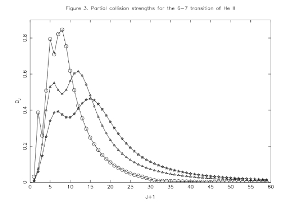
Figure 3: Partial collision strengths for the 3s ²S_1/2 - 3d ²D_3/2 (6-7) transition of He II, at three energies of: 4 Ryd (circles), 6 Ryd (triangles) and 8 Ryd (stars).

In Figs. 1-3 we show the variation of $\Omega$ with angular momentum $J$ at three energies of 4, 6 and 8 Ryd, and for three transitions, namely 2-3 (2s ²S_1/2 - 2p ²P${}^{o}_{1/2}$), 2-5 (2s ²S_1/2 - 3p ²P${}^{o}_{1/2}$) and 6-7 (3s ²S_1/2 - 3d ²D_3/2), which are ‘elastic’ (i.e. allowed with $\Delta n$ = 0), allowed ($\Delta n\neq$ 0), and forbidden, respectively. For the forbidden and allowed transitions shown in Figs. 2 and 3, the values of $\Omega$ have fully converged at all energies, including the highest energy of our calculations. However, for the ‘elastic’ transitions our range of partial waves is not sufficient for the convergence of $\Omega$, as shown in Fig. 1. For such transitions the top-up from the Coulomb-Bethe approximation is quite significant.

In Table 3 we present our results of $\Omega$ for all transitions over a wider energy range (4 $\leq$ E $\leq$ 9 Ryd), but above thresholds. The indices adopted to represent a transition are given in Table 1. These results for $\Omega$ are not directly applicable in plasma modelling, but are very useful in assessing the accuracy of a calculation. Unfortunately there are no other similar results for the fine-structure transitions, although values of $\Omega$ are available for the $LS$ transitions in the energy range 4 $\leq$ E $\leq$ 7 Ryd from our earlier calculations [2]. Therefore, we have performed another calculation using the fac code to make an accuracy assessment for the present results.

The values of $\Omega$ calculated from the fac code are listed in Table 3 at a single excited (E_j) energy of $\sim$ 5.5 Ryd, which nearly corresponds to the highest (initial) energy of our calculations, i.e. 9 Ryd. These $\Omega$ from fac provide a ready comparison with our corresponding results from darc. The two sets of $\Omega$ from darc and fac generally agree within 20% for a majority of transitions. However, for about 20% of the transitions (examples include 2-23, 3-23 and 4-23) there are differences of over 20%. In particular, six transitions, namely 1 (1s ²S_1/2) - 15 (4f ²F${}^{o}_{5/2}$), 16 (4f ²F${}^{o}_{7/2}$), 21 (5f ²F${}^{o}_{5/2}$), 23 (5g ²G_7/2), 24 (5f ²F${}^{o}_{7/2}$), and 25 (5g ²G_9/2), have larger discrepancies of up to (almost) an order of magnitude. All of these are resonance transitions but their values of $\Omega$ are very small, i.e. $\leq$ 10^-4, and hence may not affect plasma modelling applications. Such differences, for weak transitions, between the two codes are common and have been noted for a wide range of ions. They partly arise due to the different methodologies adopted (i.e. $R$-matrix and DW) and partly because the FAC code does not calculate $\Omega$ at each partial wave, but rather interpolates at regular intervals to improve efficiency. Nevertheless, for comparatively stronger transitions there is good agreement between the two independent calculations, as also illustrated in Fig. 4 for the 5-7 (3p ²P${}^{o}_{1/2}$ - 3d ²D_3/2), 6-8 (3s ²S_1/2 - 3p ²P${}^{o}_{3/2}$) and 8-9 (3p ²P${}^{o}_{3/2}$ - 3d ²D_5/2) transitions.

Table 3: Collision strengths for transitions in He II from our calculations with the DARC code. Presently calculated results from FAC are also listed at a single incident energy of $\sim$9 Ryd. ($a{\pm}b\equiv$ $a\times$10^±b).

Transition		Energy (Ryd)
$i$	$j$	4	5	6	7	8	9	FAC
1	2	1.200$-$01	1.423$-$01	1.486$-$01	1.551$-$01	1.606$-$01	1.667$-$01	1.979$-$01
1	3	1.690$-$01	2.619$-$01	3.183$-$01	3.619$-$01	4.020$-$01	4.388$-$01	4.742$-$01
1	4	3.380$-$01	5.237$-$01	6.365$-$01	7.238$-$01	8.039$-$01	8.774$-$01	9.482$-$01
1	5	3.047$-$02	5.816$-$02	6.672$-$02	7.281$-$02	7.844$-$02	8.382$-$02	8.403$-$02
1	6	3.828$-$02	3.896$-$02	3.395$-$02	3.252$-$02	3.210$-$02	3.249$-$02	3.920$-$02
1	7	1.289$-$02	1.282$-$02	1.088$-$02	1.017$-$02	9.971$-$03	9.989$-$03	7.994$-$03
1	8	6.090$-$02	1.163$-$01	1.334$-$01	1.456$-$01	1.568$-$01	1.676$-$01	1.681$-$01
1	9	1.934$-$02	1.922$-$02	1.632$-$02	1.526$-$02	1.496$-$02	1.498$-$02	1.199$-$02
1	10	1.425$-$02	2.551$-$02	2.760$-$02	2.913$-$02	3.069$-$02	3.226$-$02	3.016$-$02
……..
……..
……..

Figure 4: Comparison of collision strengths for the 5-7 (3p ²P${}^{o}_{1/2}$ - 3d ²D_3/2), 6-8 (3s ²S_1/2 - 3p ²P${}^{o}_{3/2}$) and 8-9 (3p ²P${}^{o}_{3/2}$ - 3d ²D_5/2) transitions of He II. Continuous curves are from our calculations from darc, broken curves are from the CC+CB programs, and the $\Omega$ from FAC are shown as, circles: 5-7, stars: 6-8 and squares: 8-9 transition.

However, there are four allowed transitions, namely 14-15 (4d ²D_5/2 - 4f ²F${}^{o}_{5/2}$), 19-20 (5d ²D_3/2 - 5p ²P${}^{o}_{3/2}$), 21-22 (5f ²F${}^{o}_{5/2}$ - 5d ²D_5/2), and 23-24 (5g ²G_7/2 - 5f ²F${}^{o}_{7/2}$), for which the discrepancies between the fac and darc calculations are comparatively more significant. The energy differences ($\Delta$E) for these transitions are (almost) zero in our grasp and fac calculations as shown in Table 1, and hence the correspondingly values of $\Omega$ are rather sensitive as stated in section 2. Therefore, to resolve the differences between the fac and darc calculations, and to determine values of $\Omega$ as accurately as possible, we have performed yet another calculation using the CC+CB code and the energy levels of NIST.

The results for $\Omega$ obtained from CC+CB are shown in Fig. 4 for the 5-7, 6-8 and 8-9 transitions, and agree very well with the other two calculations from darc and fac. This provides confidence in the calculated values of $\Omega$ from CC+CB. In Fig. 5 we show similar comparisons between $\Omega$ values from fac and CC+CB for three transitions, namely 14-15 (4d ²D_5/2 - 4f ²F${}^{o}_{5/2}$), 21-22 (5f ²F${}^{o}_{5/2}$ - 5d ²D_5/2) and 23-24 (5g ²G_7/2 - 5f ²F${}^{o}_{7/2}$). For these transitions there are also no (great) discrepancies between the fac and CC+CB calculations, although the FAC results are lower by $\sim$10% for 14–15. Therefore, for the 26 elastic transitions we have adopted values of $\Omega$ from our CC+CB calculations, and from darc for the remaining 274.

Figure 5: Comparison of collision strengths for the 14-15 (4d ²D_5/2 - 4f ²F${}^{o}_{5/2}$), 21-22 (5f ²F${}^{o}_{5/2}$ - 5d ²D_5/2) and 23-24 (5g ²G_7/2 - 5f ²F${}^{o}_{7/2}$) transitions of He II. Broken curves are from the CC+CB programs, and the $\Omega$ from FAC are shown as, squares: 14-15, circles: 21-22 and stars: 23-24 transition.

6 Effective collision strengths

Effective collision strengths $\Upsilon$ are obtained after integrating $\Omega$ over a Maxwellian distribution of electron velocities, i.e.

$$\Upsilon(T_{e})=\int_{0}^{\infty}{\Omega}(E)\,exp(-E_{j}/kT_{e})d(E_{j}/{kT_{e}})$$ (6)

where E_j is the incident energy of the electron with respect to the final state of the transition, $k$ is Boltzmann’s constant, and T_e is the electron temperature in K. Once the value of $\Upsilon$ is known for a transition, the corresponding value of the excitation $q(i,j)$ and de-excitation $q(j,i)$ rate coefficients can be easily obtained from the following simple relations:

$$q(i,j)=\frac{8.63\times 10^{-6}}{{\omega_{i}}{T_{e}^{1/2}}}\Upsilon\,{\rm exp}(-E_{ij}/{kT_{e}})\hskip 28.45274pt{\rm cm^{3}s^{-1}}$$ (7)

and

$$q(j,i)=\frac{8.63\times 10^{-6}}{{\omega_{j}}{T_{e}^{1/2}}}\Upsilon\hskip 28.45274pt{\rm cm^{3}s^{-1}},$$ (8)

where $\omega_{i}$ and $\omega_{j}$ are the statistical weights of the initial ($i$) and final ($j$) states, respectively, and E_ij is the transition energy.

Figure 6: Collision strengths for the 1s ²S_1/2 - 2s ²S_1/2 (1-2) transition of He II.

Figure 7: Collision strengths for the 1s ²S_1/2 - 2p ²P${}^{o}_{1/2}$ (1-3) transition of He II.

Figure 8: Collision strengths for the 2p ²P${}^{o}_{1/2}$ - 2p ²P${}^{o}_{3/2}$ (3-4) transition of He II.

Since the threshold energy region is dominated by numerous resonances, values of $\Omega$ have been computed at a large number of energies to delineate these resonances. We have performed our calculations of $\Omega$ at $\sim$ 3000 energies in the threshold region. However, the energy mesh is not uniform and varies between 0.000 01 and 0.001 Ryd. The density and importance of resonances can be appreciated from Figs. 6-8, where we show our $\Omega$ values in the thresholds region for the 1-2 (1s ²S_1/2 - 2s ²S_1/2), 1-3 (1s ²S_1/2 - 2p ²P${}^{o}_{1/2}$), and 3-4 (2p ²P${}^{o}_{1/2}$ - 2p ²P${}^{o}_{3/2}$) transitions, respectively. Resonance structure for the 1-2 transition is similar to that shown in Fig. 1 of our earlier calculations in $LS$ coupling [2], and there are only a few minor differences in the magnitudes and positions of resonances, which do not significantly affect the $\Upsilon$ results. However, the discrepancies with the measurements of Dolder and Peart [1] remain the same, i.e. the experimental results are underestimated in comparison to theory by $\sim$ 30%.

Our calculated values of $\Upsilon$ are listed in Table 4 over a wide temperature range of 3.6 $\leq$ log T${}_{e}\leq$ 5.4 K, suitable for applications to astrophysical and other plasmas. As noted in section 1, the most comprehensive similar calculations available in the literature for comparison are those of Kisielius et al. [3]. For a majority of transitions there is good agreement between the two calculations over the entire range of common temperatures, i.e. 3.2 $\leq$ log T_e (K) $\leq$ 4.3. However, six transitions (4-15, 7-14, 10-14, 10-15, 11-14, and 11-15) show discrepancies of over 20%. We illustrate this in Fig. 9 for three transitions, namely 7-14 (3d ²D_3/2 - 4d ²D_5/2), 10-15 (4p ²P${}^{o}_{1/2}$ - 4f ²F${}^{o}_{5/2}$) and 11-15 (4s ²S_1/2 - 4f ²F${}^{o}_{5/2}$). All six transitions are forbidden, but converge slowly as demonstrated in Fig. 10 for the 11-15 transition, for which the discrepancy is the greatest. As a result of slow convergence, $\Omega$ values for these transitions either decrease slowly with increasing energy or remain nearly constant, as shown in Table 3 and also verified by the FAC calculations. Since the discrepancies between our values of $\Upsilon$ and those listed by Kisielius et al. increase with increasing temperature, it appears that their calculations of $\Omega$ at higher energies are comparatively less accurate. However, as Kisielius et al. have not reported any data for collision strengths, we cannot directly verify the differences between the corresponding values of $\Upsilon$. Furthermore, an exercise performed by including only $J\leq$ 40 (i.e. the partial waves range adopted by these authors), shows a difference of less than 20% between the $\Omega$ values so obtained and those in Table 3. Therefore, the reason for the differences between the two sets of $\Upsilon$ values may lie somewhere else. We discuss this further below.

Apart from the six transitions listed above, there are three others, namely 12-14 (4d ²D_3/2 - 4d ²D_5/2), 13-15 (4p ²P${}^{o}_{3/2}$ - 4f ²F${}^{o}_{5/2}$) and 15-16 (4f ²F${}^{o}_{5/2}$ - 4f ²F${}^{o}_{7/2}$), for which the discrepancy between our results of $\Upsilon$ and those of Kisielius et al. [3] is up to two orders of magnitude over the entire range of common temperatures, with the $\Upsilon$ values of Kisielius et al. invariably higher. For these transitions, there are no discrepancies between our calculations from darc and fac, and our values of $\Upsilon$ (especially at higher temperatures) closely follow the corresponding results for $\Omega$. Therefore, we are confident that our results for $\Upsilon$ are comparatively more accurate than those of Kisielius et al.

Table 4: Effective collision strengths for transitions in He II. ($a{\pm}b\equiv a{\times}10^{{\pm}b}$).

Transition		Temperature (log Te, K)
$i$	$j$	3.60	3.80	4.00	4.20	4.40	4.60	4.80	5.00	5.20	5.40
1	2	1.713$-$01	1.689$-$01	1.661$-$01	1.629$-$01	1.595$-$01	1.553$-$01	1.502$-$01	1.458$-$01	1.432$-$01	1.417$-$01
1	3	1.141$-$01	1.162$-$01	1.191$-$01	1.229$-$01	1.281$-$01	1.349$-$01	1.445$-$01	1.597$-$01	1.831$-$01	2.118$-$01
1	4	2.264$-$01	2.311$-$01	2.371$-$01	2.449$-$01	2.555$-$01	2.692$-$01	2.885$-$01	3.190$-$01	3.660$-$01	4.233$-$01
1	5	2.232$-$02	2.306$-$02	2.398$-$02	2.482$-$02	2.589$-$02	2.795$-$02	3.157$-$02	3.679$-$02	4.309$-$02	4.897$-$02
1	6	4.615$-$02	4.616$-$02	4.619$-$02	4.558$-$02	4.439$-$02	4.309$-$02	4.198$-$02	4.095$-$02	3.970$-$02	3.777$-$02
1	7	1.967$-$02	1.905$-$02	1.853$-$02	1.785$-$02	1.695$-$02	1.601$-$02	1.518$-$02	1.444$-$02	1.369$-$02	1.277$-$02
1	8	4.415$-$02	4.574$-$02	4.767$-$02	4.942$-$02	5.161$-$02	5.576$-$02	6.304$-$02	7.350$-$02	8.613$-$02	9.789$-$02
1	9	2.964$-$02	2.867$-$02	2.786$-$02	2.680$-$02	2.543$-$02	2.402$-$02	2.277$-$02	2.166$-$02	2.053$-$02	1.915$-$02
1	10	1.626$-$02	1.492$-$02	1.399$-$02	1.362$-$02	1.394$-$02	1.498$-$02	1.664$-$02	1.867$-$02	2.082$-$02	2.248$-$02
……..
……..
……..

Figure 9: Comparison of effective collision strengths for the 7-14 (squares: 3d ²D_3/2 - 4d ²D_5/2), 10-15 (circles: 4p ²P${}^{o}_{1/2}$ - 4f ²F${}^{o}_{5/2}$) and 11-15 (stars: 4s ²S_1/2 - 4f ²F${}^{o}_{5/2}$) transitions of He II. Continuous curves are the present results from darc and broken curves are from Kisielius et al. [3].

Figure 10: Partial collision strengths for the 4s ²S_1/2 - 4f ²F${}^{o}_{5/2}$ (11-15) transition of He II, at three energies of: 4 Ryd (circles), 6 Ryd (triangles) and 8 Ryd (stars).

Figure 11: Collision strengths for the 3s ²S_1/2 - 4s ²S_1/2 (6-11) transition of He II.

Kisielius et al. [3] compared their values of $\Upsilon$ for some $LS$ transitions with our earlier calculations [2], and observed differences of up to a factor of three. For almost all the transitions in their Table 2, their values of $\Upsilon$ are not only higher but are also in agreement with the present calculations, hence confirming the inaccuracy of our earlier results in $LS$ coupling. However, they explained the differences between the two calculations on the basis of the resonances they observed near the thresholds, which we do not believe to be the correct explanation. In Table 5a we compare values of $\Omega$ from both our present and previous calculations [2] for some transitions for which the discrepancies are large. Corresponding values of $\Upsilon$ are listed in Table 5b, but only for our current work and that of Kisielius et al. Earlier results from Aggarwal et al. [2] are listed at a single temperature of 10⁴ K to provide a ready comparison. For the 1s-4s and 1s-4p transitions, the two sets of $\Omega$ agree at energies above 4 Ryd, but at E = 4 Ryd the earlier values of $\Omega$ are considerably lower. We have no explanation for this as the earlier data are no longer available. However, it does explain the smaller values of $\Upsilon$ obtained in the earlier calculations, as it affects the results more at lower temperatures than the higher ones. For the 1s-4d, 3s-4s, and 3s-4p transitions, the two sets of $\Omega$ agree over the entire common energy range of 4 $\leq$ E $\leq$ 7 Ryd, yet the earlier results for $\Upsilon$ are lower by up to a factor of two. We observe resonances for these (corresponding fine-structure) transitions, as shown in Fig. 11 for 6-11 (3s ²S_1/2 - 4s ²S_1/2). However, these (and similar other) resonances do not have a significant effect on $\Upsilon$, because the energy range of the near threshold resonances is very narrow ($<$ 0.1 Ryd). As a result, $\Upsilon$ closely follow the background values of $\Omega$ over the entire temperature range. Therefore, the differences between the $LS$ and $jj$ values of $\Upsilon$ are not due to resonances, although we are unable to fully understand these. Finally, for the 4s-4f and 4p-4f transitions, not only do our values of $\Omega$ from the earlier $LS$ calculations agree with the present work, but the corresponding $\Upsilon$ also agree. Clearly, for these two (and some other) transitions, the $\Upsilon$ values of Kisielius et al. are not only anomalous but must also be in error.

Table 5: a. Comparison of collision strengths ($\Omega$) for some transitions of He II.

Energy	4.0		5.0		6.0		7.0 Ryd
Transition	DARC	RM	DARC	RM	DARC	RM	DARC	RM
1s - 4s	0.0242	0.0157	0.0212	0.0235	0.0157	0.0159	0.0137	0.0130
1s - 4p	0.0427	0.0315	0.0765	0.0740	0.0828	0.0785	0.0874	0.0863
1s - 4d	0.0257	0.0268	0.0194	0.0199	0.0148	0.0144	0.0133	0.0133
3s - 4s	3.258	3.220	8.902	9.199	10.52	10.61	11.13	11.09
3s - 4p	4.336	4.252	13.28	13.84	19.38	22.64	23.97	29.34
4s - 4f	13.08	16.80	15.51	16.79	14.69	14.99	14.17	14.12
4p - 4f	93.03	107.0	115.6	116.0	113.1	108.0	109.3	100.7

Table 5: b. Comparison of effective collision strengths ($\Upsilon$) for some transitions of He II. ($a{\pm}b\equiv a{\times}10^{{\pm}b}$).

Transition	DARC				DRM				RM
Te (log K)	3.2	3.5	4.0	4.3	3.2	3.5	4.0	4.3	4.0
1s - 4s	3.51-2	3.03-2	2.57-2	2.46-2	3.63-2	3.11-2	2.56-2	2.44-2	8.63-3
1s - 4p	6.04-2	5.11-2	4.19-2	4.10-2	6.25-2	5.24-2	4.25-2	4.16-2	1.55-2
1s - 4d	4.41-2	3.75-2	3.06-2	2.84-2	4.54-2	3.84-2	3.06-2	2.80-2	1.56-2
3s - 4s	2.51-0	2.24-0	2.11-0	2.43-0	2.59-0	2.28-0	2.14-0	2.49-0	1.37-0
3s - 4p	7.04-0	6.47-0	5.48-0	5.08-0	7.19-0	6.57-0	5.98-0	6.14-0	2.90-0
4s - 4f	3.49+1	3.13+1	2.69+1	2.29+1	3.84+1	3.65+1	3.88+1	4.20+1	2.48+1
4p - 4f	121.1	118.0	124.5	119.1	1588	1607	1624	1602	119.9

DARC: Present calculations
DRM: Calculations of Kisielius et al. [3]
RM: Calculations of Aggarwal et al. [2]

Figure 12: Comparison of effective collision strengths for the 1-6 (squares: 1s ²S_1/2 - 3s ²S_1/2), 2-5 (circles: 2s ²S_1/2 - 3p ²P${}^{o}_{1/2}$), 2-15 (stars: 2s ²S_1/2 - 4f ²F${}^{o}_{5/2}$), and 2-16 (triangles: 2s ²S_1/2 - 4f ²F${}^{o}_{7/2}$) transitions of He II. Continuous curves are the present results from darc and broken curves are from the chianti database. Note that for clarity $\Upsilon$ for the 1–6 transition have been multiplied by a factor of 10.

The other $\Upsilon$ values available in the literature are in the chianti database, from the calculations of Ballance et al. [4], for transitions from the lowest two levels to higher excited levels. Unfortunately however, for a majority of the common transitions, there is no agreement between the two sets of $\Upsilon$. We demonstrate this in Fig. 12 for four transitions, namely 1-6 (1s ²S_1/2 - 3s ²S_1/2), 2-5 (2s ²S_1/2 - 3p ²P${}^{o}_{1/2}$), 2-15 (2s ²S_1/2 - 4f ²F${}^{o}_{5/2}$), and 2-16 (2s ²S_1/2 - 4f ²F${}^{o}_{7/2}$). Since our values of $\Upsilon$ are invariably higher, by up to 30%, it is clearly because of the inclusion of pseudostates in the expansion of the wavefunctions by Ballance et al. This process takes account of the higher ionisation channels (neglected in the present work) which results in a loss of flux, and subsequently to lower values of $\Omega$ (and hence $\Upsilon$), for some of the transitions, as also demonstrated by Aggarwal et al. [18] and Ballance et al. However, differences between our results for $\Upsilon$ and those of Ballance et al. are up to a factor of four for some transitions, such as 1-19 (1s ²S_1/2 - 5d ²D_3/2), 2-18 (2s ²S_1/2 - 5s ²S_1/2) and 2-24 (2s ²S_1/2 - 5f ²F${}^{o}_{7/2}$). For these (and some other) transitions the discrepancies between the two sets of $\Upsilon$ persist over the entire range of temperatures. However, in the absence of any results for $\Omega$ from the calculations of Ballance et al., it is difficult to arrive at any definite conclusion.

7 Conclusions

In the present work, results for energy levels, radiative rates, collision strengths, and effective collision strengths are listed for all transitions among the lowest 25 levels of He II. Radiative rates are also presented for four types of transitions, namely E1, E2, M1, and M2. This complete dataset should be useful for modelling a variety of plasmas.

Our calculations have been performed in the $jj$ coupling scheme, CI (configuration interaction) and relativistic effects included while generating wavefunctions, and a wide range of partial waves adopted to achieve convergence in $\Omega$ for a majority of transitions. Furthermore, resonances have been resolved in a fine energy mesh to improve the accuracy of the derived values of $\Upsilon$. Similarly, $\Omega$ have been computed over a wide energy range up to 9 Ryd to determine $\Upsilon$ up to a temperature of 10^5.4 K.

Three other calculations, based on the same $R$-matrix method as adopted in the present work, are available in the literature. Differences among all these calculations are significant for some of the transitions. We are able to understand and explain most of the differences, but not all, because data for collision strengths are not available for the earlier calculations. Nevertheless, based on comparisons among a variety of calculations, the accuracy of our $\Omega$ and $\Upsilon$ is probably better than 20% for a majority of transitions. However, scope remains for further improvement, mainly because we have not included pseudostates in the expansion of wavefunctions. Their inclusion in a calculation may decrease $\Upsilon$ by up to 30%, but only for some transitions, as demonstrated by Aggarwal et al. [18] and Ballance et al. [4]. Until such calculations are performed, the present values of $\Omega$ and $\Upsilon$ are not only for all transitions among the lowest 25 levels of He II, but are also probably the best currently available.

References

- [1] Dolder, K.T.; Peart, B. A measurement of cross sections for the 1S-2S excitation of He+ ions by electron impact. J. Phys. 1973, B 6, 2415.
- [2] Aggarwal, K.M.; Berrington, K.A.; Kingston, A.E.; Pathak, A. Electron collision strengths for all transitions among the =1, 2, 3, 4 and 5 levels of He+. J. Phys. 1991, B 24, 1757.
- [3] Kisielius, R.; Berrington, K.A.; Norrington, P.H. Atomic data from the IRON Project. XV. Electron excitation of the fine-structure transitions in hydrogen-like ions He II and Fe XXVI. Astron. Astrophys. Supl. 1996, 118, 157.
- [4] Ballance, C.P.; Badnell, N.R.; Smyth, E.S. A pseudo-state sensitivity study on hydrogenic ions. J. Phys. 2003, B 36, 3707.
- [5] Berrington, K.A.; Burke, P.G.; LeDourneuf, M.; Robb, W.D.; Taylor, K.T.; Vo Ky Lan. A new version of the general program to calculate atomic continuum processes using the R-matrix method. Comput. Phys. Commun. 1978, 14, 367.
- [6] Bryans, P.; Badnell, N.R.; Gorczyca, T.W.; Laming, J.M.; Mitthumsiri, W.; Savin, D.W. Collisional ionization equilibrium for optically thin plasmas. I. updated recombination rate coefficients for bare through sodium-like ions. Astrophys. J. Supl. 2006, 167, 343.
- [7] Grant, I.P.; McKenzie, B.J.; Norrington, P.H.; Mayers, D.F.; Pyper, N.C. An atomic multiconfigurational Dirac-Fock package. Comput. Phys. Commun. 1980, 21, 207.
- [8] Gu, M.F. The flexible atomic code. Can. J. Phys. 2008, 86, 675.
- [9] Aggarwal, K.M.; Hamada, K.; Igarashi, A.; Jonauskas, V.; Keenan, F.P.; Nakazaki, S. Radiative rates and electron impact excitation rates for H-like Fe XXVI. Astron. Astrophys. 2008, 484, 879.
- [10] Aggarwal, K.M.; Hamada, K.; Igarashi, A.; Jonauskas, V.; Keenan, F.P.; Nakazaki, S. Radiative rates and electron impact excitation rates for H-like Ar XVIII. Astron. Astrophys. 2008, 487, 383.
- [11] Burgess, A.; Hummer, D.G.; Tully, J. A. Electron impact excitation of positive ions. Phil. Trans. Roy. Soc. 1970, A 266, 225.
- [12] Igarashi, A.; Horiguchi, Y.; Ohsaki, A.; Nakazaki, S. Electron-impact excitations between the n=2 fine-structure levels of hydrogenic ions. J. Phys. Soc. Japan 2003, 72, 307.
- [13] Igarashi, A.; Ohsaki, A.; Nakazaki, S. Electron-exchange effect in electron-impact excitation of the n=2 fine-structure levels of hydrogenic ions. J. Phys. Soc. Japan 2005, 74, 321.
- [14] Hamada, K.; Aggarwal, K.M.; Akita, K.: Igarashi, A.; Keenan, F.P.; Nakazaki, S. Effective collision strengths for optically allowed transitions among degenerate levels of hydrogenic ions with 2 Z 30. At. Dsata Nucl. Data Tables 2010, 96, 481.
- [15] Aggarwal, K.M.; Igarashi, A.; Keenan, F.P.; Nakazaki, S. Effective collision strengths for allowed transitions among the 5 degenerate levels of Al XIII. Astron. Astrophys. 2008, 479, 585.
- [16] Parpia, F.A.; Johnson, W.R. Radiative decay rates of metastable one-electron atoms. Phys. Rev. 1982, A 26, 1142.
- [17] Pal’chikov, V.G. Relativistic transition probabilities and oscillator strengths in hydrogen-like atoms. Phys. Scr. 1998, 57, 581.
- [18] Aggarwal, K.M.; Callaway, J.; Kingston, A.E.; Unnikrishnan, K. Excitation rate coefficients for transitions among the = 1, 2 and 3 levels of He+. Asrtophys. J. Supl. 1992, 80, 473.