Controlling the Kelvin Force: Basic Strategies and Applications to Magnetic Drug Targeting

Abstract

Motivated by problems arising in magnetic drug targeting, we propose to generate an almost constant Kelvin (magnetic) force in a target subdomain, moving along a prescribed trajectory. This is carried out by solving a minimization problem with a tracking type cost functional. The magnetic sources are assumed to be dipoles and the control variables are the magnetic field intensity, the source location and the magnetic field direction. The resulting magnetic field is shown to effectively steer the drug concentration, governed by a drift-diffusion PDE, from an initial to a desired location with limited spreading.

AMS subject classification 49J20, 35Q35, 35R35, 65N30

1 Introduction

Magnetic drug targeting (MDT) is an important application of ferrofluids where drugs, with ferromagnetic particles in suspension, are injected into the body. The external magnetic field then can control the drug and subsequently the drug can target the relevant areas, for example, solid tumors (see, for instance, [22]). Mathematically this process can be modeled as follows: let the concentration of magnetic nanoparticles confined in a domain $\widetilde{\Omega}\subset\mathbb{R}^{d},d=2,3$. Let $c$ be the drug concentration and ${\bm{h}}$ the magnetic field, then the evolution of $c$ by the applied magnetic field is given by the following convection-diffusion model [14, 20]:

$$\partial_{t}c+\mathop{\mathrm{div}}\nolimits\left(-A\nabla c+({\bm{u}}+\gamma{\bm{f}}({\bm{h}}))c\right)=0\quad\mbox{in }\widetilde{\Omega}\times(0,T)$$ (1.1)

$$(-A\nabla c+({\bm{u}}+\gamma{\bm{f}}({\bm{h}}))c)\cdot\bm{n}=0\quad\mbox{on }\partial\widetilde{\Omega}\times(0,T)\qquad c(x,0)=c_{0}\quad\mbox{in }\widetilde{\Omega}$$ (1.2)

$$\mathop{\mathbf{curl}}\nolimits{\bm{h}}={\bm{0}}\quad\mbox{in }\widetilde{\Omega}\qquad\mathop{\mathrm{div}}\nolimits\mathinner{\left(\mu{\bm{h}}\right)}=0\quad\mbox{in }\widetilde{\Omega}$$ (1.3)

where $\gamma$ is a constitutive constant, $A$ is a diffusion coefficient matrix, ${\bm{u}}$ is a fixed velocity vector, $\bm{n}$ is the outward unit normal, the magnetic permeability $\mu$ is assumed to be constant, and ${\bm{f}}$ is the Kelvin force applied to a magnetic particle:

$${\bm{f}}({\bm{h}})=\nu\nabla|{\bm{h}}|^{2},$$

where $\nu>0$ is a constant depending on the volume of the particle and its permeability (see [20] for details). The two fundamental units that determine the evolution of concentration $c$ are transport and diffusion (cf. (1.1)).

The aim of magnetic drug delivery is to move a drug, initially concentrated in a small subdomain $D_{0}$ and described by the initial concentration $c_{0}$, to another suddomain $D_{t}$ (desired location) while minimizing the spreading which is characterized by the concentration $c(t)$ at time $t$. This is a challenge because magnetic fields inherently tend to disperse magnetic particles. It is known that it is not possible to concentrate magnetic nanoparticles with a static magnetic source (Earnshaw’s theorem). To understand this essential obstruction, let $D\subset\widetilde{\Omega}$ be a subdomain and observe that

$$\mathop{\mathrm{div}}\nolimits{\bm{f}}({\bm{h}})=\mathop{\mathrm{div}}\nolimits(\nabla|{\bm{h}}|^{2})=2\Delta{\bm{h}}+2|\nabla{\bm{h}}|^{2}=2|\nabla{\bm{h}}|^{2}\geq 0\quad\textrm{in }\widetilde{\Omega}$$

implies

$$\int_{\partial D}{\bm{f}}({\bm{h}})\cdot\bm{n}\,ds=\int_{D}\mathop{\mathrm{div}}\nolimits{\bm{f}}({\bm{h}})\,dx\geq 0.$$ (1.4)

This prevents the magnetic force from focussing ${\bm{f}}({\bm{h}})\cdot\bm{n}\leq 0$ on $\partial D$, a dispersion effect we could compensate for. We are thus confronted with the following question:

Is it possible to generate an appropriate magnetic force $${\bm{f}}({\bm{h}})$$ to steer a concentration to a desired location while minimizing the spreading inherent to magnetic forces? (1.5)

A first approach to tackle this problem was proposed in [20]. A feedback control of an arrangement of magnetic sources (with fixed positions) is proposed to drive a spot of distributed ferrofluid from an initial point to a target position. The authors focus on the center of mass of the concentration and its covariance matrix which measures the spreading. This leads to a constrained minimization problem where the dynamics of (1.1)-(1.2) are approximated by two coupled ordinary differential equations.

Our approach to (1.5) aims to design and study an optimization framework for steering a target subdomain $D_{t}$ from an initial to a desired location via a magnetic force ${\bm{f}}({\bm{h}})$ which is almost constant in space within $D_{t}$ and thus minimizes the drug spreading outside $D_{t}$ due to (1.4). We stress that the relative size of the diffusion coefficient matrix $A$ also influences the spreading. This paper continues the program started in [2] upon adding the following features:

1. Controls: The control variables are now the magnetic field intensity, the magnetic field direction, and the position of the magnetic dipoles, instead of just the former [2]. This provides greater flexibility and controllability of the process.

2. Final configurations: We present several non-trivial, though extremely simplified, examples for $d=2$ that allow us to assess the question of feasibility of MDT and of our approach for its development and automation. For instance, we study the issue of moving the concentration around obstacles and of magnetic injection while minimizing the spreading.

3. Advection-diffusion PDE: For the magnetic injection example, we solve (1.1) with a realistic Neumann boundary condition (1.2), instead of the Dirichlet boundary conditions as in [2]. We also consider a smaller domain than the one considered in [20, 2] which may lead to numerical oscillations as the concentration tends to go to the boundary (see [25]). In order to deal with the advection-dominant case we have adopted the edge-averaged finite element method of [30] but other alternatives such as the implicit scheme with SUPG stabilization or the explicit schemes are equally valid. Even though we do not observe oscillations in the solution, we notice a large amount of diffusion due to the upwinding nature of the scheme. This behavior makes it difficult to control the concentration in complicated geometries, for instance, the one needed to control the flow around an obstacle.

   For the second example we intend to move the concentration around an obstacle. Given that a small diffusion parameter is needed to achieve this goal, homogeneous Dirichlet boundary condition (instead of Neumann condition) is meaningful if the concentration stays away from the boundary $\partial\widetilde{\Omega}$ (see Section 6.2 for details). Moreover, in order to deal with the numerical diffusion, we consider finite element method for space discretization and the explicit Euler scheme with mass lumping for time discretization, including a correction to tackle the dispersive effects of mass lumping [15]. The resulting scheme works better than the upwind scheme.

It is worth mentioning that this approach is not only applicable for magnetic drug targeting but for many other applications where magnetic force plays a role such as: gene therapy [10], magnetized stem-cells [28], magnetic tweezers [18], lab-on-a-chip systems that include magnetic particles or fluids [13] or separation of particles [21], just to name a few.

The paper is organized as follows: in section 2 we describe the dipole approximation of the magnetic sources to be used throughout the remaining paper. Our main work begins in section 3 where we establish the optimization problems. In section 4 we discuss the numerical approximation and convergence of our discrete scheme. We provide numerical illustrations for the optimization problem in section 5.1 and conclude with a numerical scheme and several illustrative examples for (1.1)-(1.3) in section 6.

2 Dipole approximation

Let $\Omega\subset\mathbb{R}^{d}$, $d=2,3$ be open bounded fictitious domain where we intent to control the magnetic force and $T>0$ be the final time. We assume that the magnetic sources lies outside $\overline{\Omega}$, then, from the Maxwell equations it follows that the magnetic field ${\bm{h}}$ satisfies:

$$\mathop{\mathbf{curl}}\nolimits{\bm{h}} ={\bm{0}},\quad\mathop{\mathrm{div}}\nolimits{\bm{h}}=0\quad\mbox{in }\Omega,$$ (2.1)

where the last equation follows by assuming a linear relation between the magnetic induction and the magnetic field. The magnetic field generated by a current distribution and a permanent magnet can be modeled by the Biot-Savart law, which is a magnetostatic approximation. However, for simplicity, in our case we consider a dipole approximation to the magnetic source, which provides a concise and easily tractable representation of the magnetic field (see [27] for a quantification of the error associated with the dipole approximation). This approximation is commonly used for localization of objects in applications ranging from medical imaging to military. It is also extensively used in real-time control of magnetic devices in medical sciences [12, 23, 26].

From now on we will assume that the magnetic field is modeled by the superposition of a fixed number $n_{p}$ of dipoles, namely

$${\bm{h}}=\sum_{i=1}^{n_{p}}\alpha_{i}(t)\mathinner{\left(d\dfrac{\bm{r}_{i}\bm{r}_{i}^{\top}}{|\bm{r}_{i}|^{2}}-\mathbb{I}\right)}\dfrac{\widehat{{\bm{d}}_{i}}}{|\bm{r}_{i}|^{d}},$$ (2.2)

where $\bm{r}=\bm{x}-\bm{x}_{i}\in\mathbb{R}^{d}$ and $\mathbb{I}\in\mathbb{R}^{d\times d}$ is the identity matrix. In addition, $\widehat{{\bm{d}}_{i}}\in\mathbb{R}^{d}$ and $\bm{x}_{i}\in\mathbb{R}^{d}\setminus\overline{\Omega}$, $i=1,\ldots,n_{p}$, denote unit vectors and dipole positions, respectively. It is straightforward to show that the magnetic field given by (2.2) satisfies (2.1).

3 Model optimization problem

To fix ideas, we assume the time dependent domain $D_{t}$ moves along a pre-specified curve smooth curve $\mathcal{C}$ and is strictly contained in $\Omega$ for every $t\in[0,T]$. Our goal here is then to approximate a vector field $\mathbf{f}\in[\mathrm{L}^{2}(0,T;\mathrm{L}^{2}(\Omega))]^{d}$ in $D_{t}$ by the so–called Kelvin force generated by a configuration of magnetic sources. In particular, for MDT, $\mathbf{f}$ could be considered uniform on $D_{t}$. This vector field will then replace $\nabla|{\bm{h}}|^{2}$ in (1.1) and will drive the concentration to a desired location.

In [2] we propose an optimal control problem in order to study the feasibility of the dipole approximation, namely, whether we can create a Kelvin force field that allows us to control, for instance, the concentration of nanoparticles in a bounded domain $\Omega$. With this aim, a desired vector field $\mathbf{f}$ and a time dependent domain $D_{t}\subset\Omega$, $t\in[0,T]$ are assumed to be known (see Figure 1 (left)). The field $\mathbf{f}$ is approximated in $D_{t}\subset\Omega$ by the Kelvin force generated by a configuration of $n_{p}$ dipoles with fixed directions $\widehat{{\bm{d}}}_{i}$ and positions ${\bm{x}}_{i}$. Here the control is the vector magnetic field’s magnitude ${\bm{\alpha}}(t)\mathrel{\mathop{\mathchar 58\relax}}=(\alpha_{1}(t),\ldots,\alpha_{n_{p}}(t))^{T}\in\mathbb{R}^{n_{p}}$.

In this work we will approximate $\mathbf{f}\mathrel{\mathop{\mathchar 58\relax}}=(\mathrm{f}_{1},\ldots,\mathrm{f}_{d})^{\top}$ with two different dipole configurations.

3.1 Controlling intensities and directions

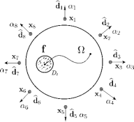
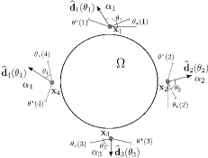
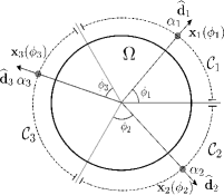
Figure 1: Left: Configuration of $n_{p}=8$ dipoles surrounding a computational domain $\Omega\subset\mathbb{R}^{2}$ and moving domain $D_{t}$. Here the target vector field $\mathbf{f}$, represented with arrows, is shown only in $D_{t}$. The center panel shows a configuration of $n_{p}=4$ dipoles with variable directions. On the right panel we show the positions $\{\bm{x}_{i}\}_{i=1}^{3}$ of the dipoles moving along the curves $\mathcal{C}_{i},i=1,2,3$, respectively. Each dipole is characterized by its position $\bm{x}_{i}$ (represented by a dot outside $\Omega$), direction ${\bm{d}}_{i}$ (represented by an arrow) and the magnitude ${\bm{\alpha}}_{i}$, for $i=1,\ldots,n_{p}$.

First we consider fixed dipole positions $\left\{\bm{x}_{i}\right\}_{i=1}^{n_{p}}$ and the controls are the magnitudes $\left\{\alpha_{i}\right\}_{i=1}^{n_{p}}$ and directions $\big{\{}\widehat{{\bm{d}}}_{i}\big{\}}_{i=1}^{n_{p}}$ parametrized by one degree of freedom per dipole (see Figure 1 (center)), namely, if ${\bm{\alpha}}(t)\mathrel{\mathop{\mathchar 58\relax}}=(\alpha_{1}(t),\ldots,\alpha_{n_{p}}(t))^{\top}\in\mathbb{R}^{n_{p}}$ and ${\bm{\theta}}(t)\mathrel{\mathop{\mathchar 58\relax}}=(\theta_{1}(t),\ldots,\theta_{n_{p}}(t))^{\top}\in\mathbb{R}^{n_{p}}$ denote the vectors of magnetic field’s magnitude and “angles”, such that $\widehat{{\bm{d}}}_{i}=\widehat{{\bm{d}}}_{i}(\theta_{i})$ for a regular function $\widehat{{\bm{d}}}_{i}$ (for instance, $\widehat{{\bm{d}}}_{i}(\theta_{i})=\left(\cos(\theta_{i}),\sin(\theta_{i})\right)$ when $d=2$), then we want to study the problem

$$\min_{({\bm{\alpha}},{\bm{\theta}})\in\mathcal{H}_{ad}\times\mathcal{V}_{ad}}\mathcal{J}({\bm{h}}({\bm{\alpha}},{\bm{\theta}}))$$ (3.1a)

with

$$\mathcal{J}({\bm{h}}({\bm{\alpha}},{\bm{\theta}}))=\dfrac{1}{2}\int_{0}^{T}\|\nabla|{\bm{h}}|^{2}-\mathbf{f}\|^{2}_{\mathrm{L}^{2}(D_{t})}+\dfrac{\lambda}{2}\int_{0}^{T}|\partial_{t}{\bm{\alpha}}|^{2}+\dfrac{\eta}{2}\int_{0}^{T}|\partial_{t}{\bm{\theta}}|^{2}$$ (3.1b)

and

$${\bm{h}}({\bm{\alpha}},{\bm{\theta}})=\sum_{i=1}^{n_{p}}\alpha_{i}(t)\mathinner{\left(d\dfrac{\bm{r}_{i}\bm{r}_{i}^{\top}}{|\bm{r}_{i}|^{2}}-\mathbb{I}\right)}\dfrac{\widehat{{\bm{d}}_{i}}(\theta_{i})}{|\bm{r}_{i}|^{d}},$$ (3.1c)

and where $({\bm{\alpha}},{\bm{\theta}})\in\mathcal{H}_{ad}\times\mathcal{V}_{ad}$ and $\lambda$ and $\eta$ are the costs of the control. For given constant vectors ${\bm{\alpha}}_{0},{\bm{\theta}}_{0},{\bm{\alpha}}_{*},{\bm{\theta}}_{*},{\bm{\alpha}}^{*},{\bm{\theta}}^{*}\in\mathbb{R}^{n_{p}}$, we seek $({\bm{\alpha}},{\bm{\theta}})$ in the following admissible convex sets:

$$\mathcal{H}_{ad}\mathrel{\mathop{\mathchar 58\relax}}=\left\{{\bm{\alpha}}\in[\mathrm{H}^{1}(0,T)]^{n_{p}}\mathrel{\mathop{\mathchar 58\relax}}{\bm{\alpha}}(0)={\bm{\alpha}}_{0},\,\,\mbox{and}\,\,{\bm{\alpha}}_{*}\leq{\bm{\alpha}}(t)\leq{\bm{\alpha}}^{*},\,\,\forall t\in[0,T]\right\}$$

and

$$\mathcal{V}_{ad}\mathrel{\mathop{\mathchar 58\relax}}=\left\{{\bm{\theta}}\in[\mathrm{H}^{1}(0,T)]^{n_{p}}\mathrel{\mathop{\mathchar 58\relax}}{\bm{\theta}}(0)={\bm{\theta}}_{0},\,\,\mbox{and}\,\,{\bm{\theta}}_{*}\leq{\bm{\theta}}(t)\leq{\bm{\theta}}^{*},\forall\,t\in[0,T]\right\}.$$

Notice that, in view of (3.1c), we can rewrite ${\bm{h}}$ as ${\bm{h}}({\bm{\alpha}},{\bm{\theta}})=\mathbb{D}({\bm{\theta}}){\bm{\alpha}}$ where

$$\mathbb{D}({\bm{\theta}})=\big{(}{\bm{D}}_{1}(\theta_{1})\,{\bm{D}}_{2}(\theta_{2})\,\ldots\,{\bm{D}}_{n_{p}}(\theta_{n_{p}})\big{)}\in[\mathrm{H}^{1}(0,T;C^{\infty}(\overline{\Omega}))]^{d\times{n_{p}}}$$

is such that

$${\bm{D}}_{i}(\theta_{i})\mathrel{\mathop{\mathchar 58\relax}}=\mathinner{\left(d\dfrac{(\bm{x}-\bm{x}_{i})(\bm{x}-\bm{x}_{i})^{\top}}{|\bm{x}-\bm{x}_{i}|^{2}}-\mathbb{I}\right)}\dfrac{\widehat{{\bm{d}}_{i}}(\theta_{i})}{|\bm{x}-\bm{x}_{i}|^{d}}=\mathbb{M}_{i}(\bm{x})\widehat{{\bm{d}}_{i}}(\theta_{i}).$$

Thus, the Kelvin force in terms of ${\bm{\alpha}}$ and ${\bm{\theta}}$ is given by

$$\nabla|{\bm{h}}|^{2} =\nabla\left({\bm{\alpha}}(t)^{\top}(\mathbb{D}({\bm{\theta}})^{\top}\mathbb{D}({\bm{\theta}})){\bm{\alpha}}(t)\right)$$

$$=\begin{pmatrix}{\bm{\alpha}}(t)^{\top}\partial_{x_{1}}(\mathbb{D}({\bm{\theta}})^{\top}\mathbb{D}({\bm{\theta}})){\bm{\alpha}}(t)\\ \vdots\\ {\bm{\alpha}}(t)^{\top}\partial_{x_{d}}(\mathbb{D}({\bm{\theta}})^{\top}\mathbb{D}({\bm{\theta}})){\bm{\alpha}}(t)\end{pmatrix}=\begin{pmatrix}{\bm{\alpha}}^{\top}\mathbb{B}_{1}({\bm{\theta}}){\bm{\alpha}}\\ \vdots\\ {\bm{\alpha}}^{\top}\mathbb{B}_{d}({\bm{\theta}}){\bm{\alpha}}\end{pmatrix}$$ (3.2)

with $\mathbb{B}_{k}({\bm{\theta}})\mathrel{\mathop{\mathchar 58\relax}}=\partial_{x_{k}}(\mathbb{D}^{\top}({\bm{\theta}})\mathbb{D}({\bm{\theta}}))\in[\mathrm{H}^{1}(0,T;C^{\infty}(\overline{\Omega}))]^{{n_{p}}\times{n_{p}}}$.

3.2 Controlling intensities and positions

For the second configuration we consider fixed dipole directions $\big{\{}\widehat{{\bm{d}}}_{i}\big{\}}_{i=1}^{n_{p}}$ and the controls are the magnitudes $\left\{\alpha_{i}\right\}_{i=1}^{n_{p}}$ and positions $\left\{\bm{x}_{i}\right\}_{i=1}^{n_{p}}$. In this case, we assume that each dipole $i$ moves along a prescribed trajectory $\mathcal{C}_{i}$ parameterized by a $C^{1}([0,T])$ curve $\bm{\rho}_{i}\mathrel{\mathop{\mathchar 58\relax}}[{\bm{\phi}}_{*}(i),{\bm{\phi}}^{*}(i)]\to\mathcal{C}_{i}$, $i=1,\ldots,n_{p}$ where ${\bm{\phi}}_{*},{\bm{\phi}}^{*}\in\mathbb{R}^{n_{p}}$ (see Figure 1 (right)). Thus, we study the problem

$$\min_{({\bm{\alpha}},{\bm{\phi}})\in\mathcal{H}_{ad}\times\mathcal{U}_{ad}}\mathcal{F}({\bm{h}}({\bm{\alpha}},{\bm{\phi}}))$$ (3.3a)

with

$$\mathcal{F}({\bm{h}}({\bm{\alpha}},{\bm{\phi}}))=\dfrac{1}{2}\int_{0}^{T}\|\nabla|{\bm{h}}|^{2}-\mathbf{f}\|^{2}_{\mathrm{L}^{2}(D_{t})}+\dfrac{\lambda}{2}\int_{0}^{T}|\partial_{t}{\bm{\alpha}}|^{2}+\dfrac{\beta}{2}\int_{0}^{T}|\partial_{t}{\bm{\phi}}|^{2}$$ (3.3b)

and

$${\bm{h}}({\bm{\alpha}},{\bm{\phi}})=\sum_{i=1}^{n_{p}}\alpha_{i}(t)\mathinner{\left(d\dfrac{\bm{r}_{i}(\phi_{i})\bm{r}_{i}(\phi_{i})^{\top}}{|\bm{r}_{i}(\phi_{i})|^{2}}-\mathbb{I}\right)}\dfrac{\widehat{{\bm{d}}_{i}}}{|\bm{r}_{i}(\phi_{i})|^{d}},$$ (3.3c)

where $\bm{r}_{i}(\phi_{i})=(\bm{x}-\bm{\rho}_{i}(\phi_{i}))$, ${\bm{\phi}}=(\phi_{1},\ldots,\phi_{n_{p}})$, $({\bm{\alpha}},{\bm{\phi}})\in\mathcal{H}_{ad}\times\mathcal{U}_{ad}$ and, for a given constant vector ${\bm{\phi}}_{0}\in\mathbb{R}^{n_{p}}$, we consider the admissible set $\mathcal{U}_{ad}\mathrel{\mathop{\mathchar 58\relax}}=\big{\{}{\bm{\phi}}\in[\mathrm{H}^{1}(0,T)]^{n_{p}}\mathrel{\mathop{\mathchar 58\relax}}{\bm{\phi}}(0)={\bm{\phi}}_{0},\,\,\mbox{and}\,\,{\bm{\phi}}_{*}\leq{\bm{\phi}}(t)\leq{\bm{\phi}}^{*},\,\,\forall t\in[0,T]\big{\}}$. We first notice that, in view of (3.3c), we can rewrite ${\bm{h}}$ as ${\bm{h}}({\bm{\alpha}},{\bm{\phi}})=\mathbb{R}({\bm{\phi}}){\bm{\alpha}}$ where $\mathbb{R}({\bm{\phi}})=\left({\bm{R}}_{1}(\phi_{1})\,{\bm{R}}_{2}(\phi_{2})\,\ldots\,{\bm{R}}_{n_{p}}(\phi_{n_{p}})\right)$ belongs to $[\mathrm{H}^{1}(0,T;C^{\infty}(\overline{\Omega}))]^{d\times{n_{p}}}$ and is given by

$${\bm{R}}_{i}(\phi_{i})\mathrel{\mathop{\mathchar 58\relax}}=\mathinner{\left(d\dfrac{\bm{r}_{i}(\phi_{i})\bm{r}_{i}(\phi_{i})^{\top}}{|\bm{r}_{i}(\phi_{i})|^{2}}-\mathbb{I}\right)}\dfrac{\widehat{{\bm{d}}_{i}}}{|\bm{r}_{i}(\phi_{i})|^{d}},$$

therefore, we can write the Kelvin force in terms of ${\bm{\alpha}}$ and ${\bm{\phi}}$ as follows

$$\nabla|{\bm{h}}|^{2} =\nabla\left({\bm{\alpha}}(t)^{\top}(\mathbb{R}({\bm{\phi}})^{\top}\mathbb{R}({\bm{\phi}})){\bm{\alpha}}(t)\right)$$

$$=\begin{pmatrix}{\bm{\alpha}}(t)^{\top}\partial_{x_{1}}(\mathbb{R}({\bm{\phi}})^{\top}\mathbb{R}({\bm{\phi}})){\bm{\alpha}}(t)\\ \vdots\\ {\bm{\alpha}}(t)^{\top}\partial_{x_{d}}(\mathbb{R}({\bm{\phi}})^{\top}\mathbb{R}({\bm{\phi}})){\bm{\alpha}}(t)\end{pmatrix}=\begin{pmatrix}{\bm{\alpha}}^{\top}\mathbb{G}_{1}({\bm{\phi}}){\bm{\alpha}}\\ \vdots\\ {\bm{\alpha}}^{\top}\mathbb{G}_{d}({\bm{\phi}}){\bm{\alpha}}\end{pmatrix}$$ (3.4)

with $\mathbb{G}_{k}({\bm{\phi}})\mathrel{\mathop{\mathchar 58\relax}}=\partial_{x_{k}}(\mathbb{R}^{\top}({\bm{\phi}})\mathbb{R}({\bm{\phi}}))\in[\mathrm{H}^{1}(0,T;C^{\infty}(\overline{\Omega}))]^{{n_{p}}\times{n_{p}}}$, $k=1,\ldots,d$. We will show existence of solution to problems (3.1) and (3.3) via a minimizing sequence argument (see, for instance, [29]). The feasibility of the dipole approximation can be studied with the first term of $\mathcal{J}({\bm{h}}({\bm{\alpha}},{\bm{\theta}}))$ and $\mathcal{F}({\bm{h}}({\bm{\alpha}},{\bm{\phi}}))$, because the computed Kelvin force can be used to control a desired concentration. On the other hand, the last two terms in (3.1b) (and (3.3b)) will enforce a smooth evolution of the intensities and angles (and positions).

3.3 Existence and optimality conditions

Next, we focus on the existence of a solution to the minimization problem (3.1), which is nonconvex. For notational simplicity, from now on we denote by $\mathrm{V}$ both a Banach space $\mathrm{V}$ and the Banach tensor product $\mathrm{V}^{n_{p}}$.

Theorem 1 (existence of minimizers).

There exist at least one solution $(\bar{{\bm{\alpha}}},\bar{{\bm{\theta}}})$ to the minimization problem (3.1).

Proof.

We apply the direct method of the calculus of variations. Given that $\mathcal{J}$ is bounded below by zero, we deduce that $j=\inf_{({\bm{\alpha}},{\bm{\theta}})\in\mathcal{H}_{ad}\times\mathcal{V}_{ad}}\mathcal{J}({\bm{\alpha}},{\bm{\theta}})$ is finite. We can thus construct a minimizing sequence $\{({\bm{\alpha}}_{n},{\bm{\theta}}_{n})\}_{n\in\mathbb{N}}$ such that

$$j=\lim_{n\rightarrow\infty}\mathcal{J}({\bm{\alpha}}_{n},{\bm{\theta}}_{n}).$$

As the sequence $\{({\bm{\alpha}}_{n},{\bm{\theta}}_{n})\}_{n\in\mathbb{N}}$ is uniformly bounded in $\mathcal{H}_{ad}\times\mathcal{V}_{ad}\subset[\mathrm{H}^{1}(0,T)]^{2}$, we can extract a (not relabeled) weakly convergent subsequence $\{{\bm{\alpha}}_{n}\}_{n\in\mathbb{N}}$ such that

$${\bm{\alpha}}_{n}\rightharpoonup\bar{{\bm{\alpha}}}\quad\mbox{in }\mathrm{H}^{1}(0,T),\quad\bar{{\bm{\alpha}}}\in\mathcal{H}_{ad}\quad\mbox{and}\quad{\bm{\theta}}_{n}\rightharpoonup\bar{{\bm{\theta}}}\quad\mbox{in }\mathrm{H}^{1}(0,T),\quad\bar{{\bm{\theta}}}\in\mathcal{V}_{ad}.$$ (3.5)

Moreover, according to [5, Theorem 9.16] we have

$${\bm{\alpha}}_{n}\to\bar{{\bm{\alpha}}}\quad\mbox{and }\quad{\bm{\theta}}_{n}\to\bar{{\bm{\theta}}}\quad\mbox{in }C([0,T]).$$ (3.6)

To show the optimality of $\bar{{\bm{\alpha}}}$, we first consider (3.6) to get that

$$\int_{0}^{T}\|\nabla|{\bm{h}}({\bm{\alpha}}_{n},{\bm{\theta}}_{n})|^{2}-\mathrm{f}_{i}\|^{2}_{\mathrm{L}^{2}(D_{t})}\to\int_{0}^{T}\|\nabla|{\bm{h}}(\bar{{\bm{\alpha}}},\bar{{\bm{\theta}}})|^{2}-\mathrm{f}_{i}\|^{2}_{\mathrm{L}^{2}(D_{t})}\qquad i=1,\ldots,d,$$ (3.7)

which follows from (3.1) and the fact that

$$\mathbb{B}_{k}({\bm{\theta}}_{n})_{i,j}-\mathbb{B}_{k}(\bar{{\bm{\theta}}})_{i,j}=(\widehat{{\bm{d}}}^{\top}_{i}({\bm{\theta}}_{n}(i))-\widehat{{\bm{d}}}^{\top}_{i}(\bar{{\bm{\theta}}}(i)))\left(\partial_{x_{k}}(\mathbb{M}_{i}(\bm{x})^{\top}\mathbb{M}_{j}(\bm{x}))\right)\widehat{{\bm{d}}}_{j}({\bm{\theta}}_{n}(j))\\ \widehat{{\bm{d}}}^{\top}_{i}(\bar{{\bm{\theta}}}(i))\left(\partial_{x_{k}}(\mathbb{M}_{i}(\bm{x})^{\top}\mathbb{M}_{j}(\bm{x}))\right)(\widehat{{\bm{d}}}_{j}({\bm{\theta}}_{n}(j))-\widehat{{\bm{d}}}_{j}(\bar{{\bm{\theta}}}(j))).$$

and $\widehat{{\bm{d}}_{i}}({\bm{\theta}}_{n}(i))\to\widehat{{\bm{d}}_{i}}(\bar{{\bm{\theta}}}(i))$ in $[C([0,T])]^{d}$, $i=1,\ldots,n_{p}$. Notice that here we have used, for instance, ${\bm{\theta}}(i)$ to denote the $i$-th component of vector ${\bm{\theta}}$. This and the fact that the last terms in $\mathcal{J}$ are weakly lower semicontinuous (see [29, Theorem 2.12]) yields

$$\min_{({\bm{\alpha}},{\bm{\theta}})\in\mathcal{H}_{ad}\times\mathcal{V}_{ad}}\mathcal{J}({\bm{\alpha}},{\bm{\theta}})=\liminf_{n\to\infty}\mathcal{J}({\bm{\alpha}}_{n},{\bm{\theta}}_{n})\geq\mathcal{J}(\bar{{\bm{\alpha}}},\bar{{\bm{\theta}}}),$$

which concludes the proof. ∎

By applying the same technique as above and using that $\bm{\rho}$ belongs to $C^{1}([0,T])$, we obtain the following existence result for problem (3.3).

Theorem 2 (existence of minimizers).

There exist at least one solution $(\bar{{\bm{\alpha}}},\bar{{\bm{\phi}}})$ to the minimization problem (3.3).

3.4 First order optimality conditions

To state first order optimality conditions we follow standard arguments because of the fact that $\mathcal{J}\mathrel{\mathop{\mathchar 58\relax}}[\mathrm{H}^{1}(0,T)]^{2}\rightarrow\mathbb{R}$ is Fréchet differentiable. We first notice that, in view of (2.2), we can also rewrite ${\bm{h}}$ as

$${\bm{h}}({\bm{\alpha}},{\bm{\theta}})=\sum_{i=1}^{n_{p}}\mathbb{{\bm{A}}}(\alpha_{j})\widehat{{\bm{d}}}_{j}(\theta_{j})$$

where $\mathbb{{\bm{A}}}(\alpha_{i})\in[\mathrm{H}^{1}(0,T;C^{\infty}(\overline{\Omega}))]^{d\times d}$ and is given by

$$\mathbb{{\bm{A}}}(\alpha_{i})\mathrel{\mathop{\mathchar 58\relax}}=\alpha_{i}\mathinner{\left(d\dfrac{(\bm{x}-\bm{x}_{i})(\bm{x}-\bm{x}_{i})^{\top}}{|\bm{x}-\bm{x}_{i}|^{2}}-\mathbb{I}\right)}\dfrac{1}{|\bm{x}-\bm{x}_{i}|^{d}},\quad i=1,\ldots,n_{p}.$$

Thus, the Kelvin force in terms of ${\bm{\alpha}}$ and ${\bm{\theta}}$ can be written as follows

$$\nabla|{\bm{h}}|^{2} =\sum_{m,n=1}^{n_{p}}\nabla\left(\widehat{{\bm{d}}}^{\top}_{m}(\theta_{m})(\mathbb{{\bm{A}}}^{\top}(\alpha_{m})\mathbb{{\bm{A}}}(\alpha_{n}))\widehat{{\bm{d}}}_{n}(\theta_{n})\right)$$

$$=\sum_{m,n=1}^{n_{p}}\begin{pmatrix}\widehat{{\bm{d}}}^{\top}_{m}(\theta_{m})\mathbb{Q}_{1}(\alpha_{m},\alpha_{n})\widehat{{\bm{d}}}_{n}(\theta_{n})\\ \vdots\\ \widehat{{\bm{d}}}^{\top}_{m}(\theta_{m})\mathbb{Q}_{d}(\alpha_{m},\alpha_{n})\widehat{{\bm{d}}}_{n}(\theta_{n})\end{pmatrix}$$

with $\mathbb{Q}_{k}(\alpha_{m},\alpha_{n})\mathrel{\mathop{\mathchar 58\relax}}=\partial_{x_{k}}(\mathbb{{\bm{A}}}^{\top}(\alpha_{m})\mathbb{{\bm{A}}}(\alpha_{n}))\in[\mathrm{H}^{1}(0,T;C^{\infty}(\overline{\Omega}))]^{d\times d}$ for $k=1,\ldots,d$.

Theorem 3 (first order optimality condition for $\mathcal{J}$).

If $(\bar{{\bm{\alpha}}},\bar{{\bm{\theta}}})\in\mathcal{H}_{ad}\times\mathcal{V}_{ad}$ denotes an optimal control, given by Theorem 1, then the first order necessary optimality condition satisfied by $(\bar{{\bm{\alpha}}},\bar{{\bm{\theta}}})$ is

$$\mathcal{J}^{\prime}(\bar{{\bm{\alpha}}},\bar{{\bm{\theta}}})\left\langle{\bm{\alpha}}-\bar{{\bm{\alpha}}},{\bm{\theta}}-\bar{{\bm{\theta}}}\right\rangle\geq 0\qquad\forall({\bm{\alpha}},{\bm{\theta}})\in\mathcal{H}_{ad}\times\mathcal{V}_{ad}$$

where, for $(\delta{\bm{\alpha}},\delta{\bm{\theta}})=({\bm{\alpha}}-\bar{{\bm{\alpha}}},{\bm{\theta}}-\bar{{\bm{\theta}}})$ we have

$$\mathcal{J}^{\prime}(\bar{{\bm{\alpha}}},\bar{{\bm{\theta}}}) \left\langle\delta{\bm{\alpha}},\delta{\bm{\theta}}\right\rangle=\int_{0}^{T}\Bigg{(}\sum_{i=1}^{d}\int_{D_{t}}\left(\bar{{\bm{\alpha}}}^{\top}\mathbb{B}_{i}(\bar{{\bm{\theta}}})\bar{{\bm{\alpha}}}-\mathrm{f}_{i}\right)\left(2\bar{{\bm{\alpha}}}^{\top}\mathbb{B}_{i}(\bar{{\bm{\theta}}})\delta{\bm{\alpha}}\right)d\bm{x}$$

$$+\sum_{i=1}^{d}\int_{D_{t}}\left(\bar{{\bm{\alpha}}}^{\top}\mathbb{B}_{i}(\bar{{\bm{\theta}}})\bar{{\bm{\alpha}}}-\mathrm{f}_{i}\right)\left(2\sum_{m,n=1}^{n_{p}}(\widehat{{\bm{d}}}^{\top}_{m})^{\prime}(\theta_{m})\mathbb{Q}_{i}(\alpha_{m},\alpha_{n})\widehat{{\bm{d}}}_{n}(\theta_{n})\delta\theta_{m}\right)d\bm{x}$$

$$+\lambda d_{t}\bar{{\bm{\alpha}}}^{\top}d_{t}\delta{\bm{\alpha}}+\eta d_{t}\bar{{\bm{\theta}}}^{\top}d_{t}\delta{\bm{\theta}}\Bigg{)}dt.$$

Similarly, we obtain the first order optmimality conditions for $\mathcal{F}$.

Theorem 4 (first order optimality condition for $\mathcal{F}$).

If $(\bar{{\bm{\alpha}}},\bar{{\bm{\phi}}})\in\mathcal{H}_{ad}\times\mathcal{U}_{ad}$ denotes an optimal control, given by Theorem 2, then the first order necessary optimality condition satisfied by $(\bar{{\bm{\alpha}}},\bar{{\bm{\phi}}})$ is

$$\mathcal{F}^{\prime}(\bar{{\bm{\alpha}}},\bar{{\bm{\phi}}})\left\langle{\bm{\alpha}}-\bar{{\bm{\alpha}}},{\bm{\phi}}-\bar{{\bm{\phi}}}\right\rangle\geq 0\qquad\forall({\bm{\alpha}},{\bm{\phi}})\in\mathcal{H}_{ad}\times\mathcal{V}_{ad}$$

where, for $(\delta{\bm{\alpha}},\delta{\bm{\phi}})=({\bm{\alpha}}-\bar{{\bm{\alpha}}},{\bm{\phi}}-\bar{{\bm{\phi}}})$ we have

$$\mathcal{F}^{\prime}(\bar{{\bm{\alpha}}},\bar{{\bm{\phi}}})\left\langle\delta{\bm{\alpha}},\delta{\bm{\phi}}\right\rangle= \int_{0}^{T}\Bigg{(}\sum_{i=1}^{d}\int_{D_{t}}\left(\bar{{\bm{\alpha}}}^{\top}\mathbb{G}_{i}(\bar{{\bm{\phi}}})\bar{{\bm{\alpha}}}-\mathrm{f}_{i}\right)\left(2\bar{{\bm{\alpha}}}^{\top}\mathbb{G}_{i}(\bar{{\bm{\phi}}})\delta{\bm{\alpha}}\right)d\bm{x}$$

$$+\sum_{i=1}^{d}\int_{D_{t}}\left(\bar{{\bm{\alpha}}}^{\top}\mathbb{G}_{i}(\bar{{\bm{\phi}}})\bar{{\bm{\alpha}}}-\mathrm{f}_{i}\right)\left(\sum_{l=1}^{n_{p}}\bar{{\bm{\alpha}}}^{\top}\mathbb{G}_{i}({\bm{\phi}})^{\prime}\left\langle\delta{\bm{\phi}}_{l}\right\rangle\bar{{\bm{\alpha}}}\right)d\bm{x}$$

$$+\lambda d_{t}\bar{{\bm{\alpha}}}^{\top}d_{t}\delta{\bm{\alpha}}+\beta d_{t}\bar{{\bm{\phi}}}^{\top}d_{t}\delta{\bm{\phi}}\Bigg{)}dt.$$

Remark 5 (unknown final time).

In some applications an important quantity to account for is the time it takes for $D_{t}$ to arrive at its final destination. In this case, the final time is an unknown. This problem can be handled, following [20], by reformulating the minimization in terms of the arc length which has a fixed final value. This approach can be applied to problems (3.1) and (3.3), for details see [2].

4 Discretization

In this section we propose and study a numerical approximation of minimization problems (3.1) and (3.3). We introduce a parametrization of the moving domain $D_{t}$ in terms of a fixed domain $\widehat{D}\subset\mathbb{R}^{d}$ (see also [2]). With this in mind, we define a map $\mathbf{X}\mathrel{\mathop{\mathchar 58\relax}}[0,T]\times\overline{\widehat{D}}\to\overline{\Omega}$, such that for all $t\in[0,T]$

$$\mathbf{X}(t,\cdot)\mathrel{\mathop{\mathchar 58\relax}} \overline{\widehat{D}}\to\overline{D}_{t}$$

$$\widehat{\bm{x}}\to\bm{x}=\mathbf{X}(t,\widehat{\bm{x}}),$$

is a one-to-one correspondence which satisfies $\mathbf{X}(t,\widehat{D})=D_{t}$. For simplicity, we assume

$$\mathbf{X}(t,\widehat{\bm{x}})=\bm{\varphi}(t)+\psi(t)\widehat{\bm{x}},$$

where

$$\bm{\varphi}\mathrel{\mathop{\mathchar 58\relax}}[0,T]\to\mathbb{R}^{d},\,\quad\psi\mathrel{\mathop{\mathchar 58\relax}}[0,T]\to(0,+\infty),\quad\bm{\varphi},\psi\in\mathrm{H}^{1}(0,T)$$ (4.1)

are functions such that $\bm{\varphi}(0)=\bm{0}$ and $\psi(0)=1$, namely $\widehat{D}=D_{0}$. In case $\psi(t)=\widehat{\psi}\in\mathbb{R}^{+}$ for all $t\in[0,T]$, $\bm{\varphi}$ can be viewed as a parameterization of a desired path that the scaled domain $\widehat{\psi}\widehat{D}$ traverses from an initial position to a final position.

4.1 Problem 1: Controlling intensities and directions

We consider the previous parametrization and rewrite the minimization problem (3.1) in terms of $\widehat{D}$. Therefore, for $i=1,\dots,d$

$$\int_{0}^{T}\int_{D_{t}} \left(\nabla|{\bm{h}}({\bm{\alpha}},{\bm{\theta}})|^{2}-\mathbf{f}(t,\bm{x})\right)^{2}d\bm{x}\,dt$$

$$= \sum_{i=1}^{d}\int_{0}^{T}\int_{D_{t}}\left({\bm{\alpha}}(t)^{\top}\mathbb{B}_{i}({\bm{\theta}},\bm{x}){\bm{\alpha}}(t)-\mathrm{f}_{i}(t,\bm{x})\right)^{2}d\bm{x}\,dt$$

$$= \sum_{i=1}^{d}\int_{0}^{T}\int_{\widehat{D}}\left({\bm{\alpha}}(t)^{\top}\mathbb{B}_{i}({\bm{\theta}},\mathbf{X}(t,\widehat{\bm{x}}))\psi(t)^{d/2}{\bm{\alpha}}(t)-\mathrm{f}_{i}(t,\mathbf{X}(t,\widehat{\bm{x}}))\psi(t)^{d/2}\right)^{2}d\widehat{\bm{x}}\,dt,$$

because $\det(\nabla_{\widehat{\bm{x}}}\mathbf{X}(t,\widehat{\bm{x}}))=\psi(t)^{d}$. Then, we rewrite $\mathcal{J}$ as

$$\mathcal{J}({\bm{\alpha}},{\bm{\theta}})= \dfrac{1}{2}\sum_{i=1}^{d}\int_{0}^{T}\|{\bm{\alpha}}^{\top}\widehat{\mathbb{B}}_{i}({\bm{\theta}}){\bm{\alpha}}-\widehat{\mathrm{f}}_{i}\|^{2}_{\mathrm{L}^{2}(\widehat{D})}+\dfrac{\lambda}{2}\int_{0}^{T}|d_{t}{\bm{\alpha}}|^{2}+\dfrac{\eta}{2}\int_{0}^{T}|d_{t}{\bm{\theta}}|^{2}$$

$$= \mathcal{J}^{1}({\bm{\alpha}},{\bm{\theta}})+\mathcal{J}^{2}({\bm{\alpha}})+\mathcal{J}^{3}({\bm{\theta}})$$ (4.2)

with $\widehat{\mathbb{B}}_{i}({\bm{\theta}},\widehat{\bm{x}})\mathrel{\mathop{\mathchar 58\relax}}=\mathbb{B}_{i}({\bm{\theta}},\mathbf{X}(t,\widehat{\bm{x}}))\psi(t)^{d/2}$ and $\widehat{\mathrm{f}}_{i}(t,\widehat{\bm{x}})=\mathrm{f}_{i}(t,\mathbf{X}(t,\widehat{\bm{x}}))\psi(t)^{d/2}$, $i=1,\dots,d$.

Next, we introduce a time discretization of problem (3.1) upon using $\mathcal{J}$ as defined in (4.1). Let us fix $N\in\mathbb{N}$ and let $\tau\mathrel{\mathop{\mathchar 58\relax}}=T/N$ be the time step. Now, for $n=1,\ldots,N$, we define $t^{n}\mathrel{\mathop{\mathchar 58\relax}}=n\tau$, $\widehat{\mathbb{B}}^{n}_{i}(\cdot)=\widehat{\mathbb{B}}_{i}(\cdot,\mathbf{X}(t^{n},\widehat{\bm{x}}))$ and $\widehat{\mathrm{f}}^{n}_{i}$ to be

$$\widehat{\mathrm{f}}^{n}_{i}(\cdot)=\dfrac{1}{\tau}\int_{t^{n-1}}^{t^{n}}\widehat{\mathrm{f}}_{i}(t,\cdot)dt,\qquad i=1,\ldots,d,$$ (4.3)

which in turn allows us to incorporate a general $\mathbf{f}$. Then we consider a time discrete version of (3.1): given the initial condition $({\bm{\alpha}}_{0},{\bm{\theta}}_{0})=\mathrel{\mathop{\mathchar 58\relax}}({\bm{\alpha}}_{\tau}(0),{\bm{\theta}}_{\tau}(0))$, find $(\bar{{\bm{\alpha}}}_{\tau},\bar{{\bm{\theta}}}_{\tau})\in\mathcal{H}^{\tau}_{ad}\times\mathcal{V}^{\tau}_{ad}$ solving

$$(\bar{{\bm{\alpha}}}_{\tau},\bar{{\bm{\theta}}}_{\tau})=\operatorname*{arg\,min}_{({\bm{\alpha}}_{\tau},{\bm{\theta}}_{\tau})\in\mathcal{H}^{\tau}_{ad}\times\mathcal{V}^{\tau}_{ad}}\mathcal{J}_{\tau}({\bm{\alpha}}_{\tau},{\bm{\theta}}_{\tau}),$$ (4.4)

where

$$\mathcal{J}_{\tau}({\bm{\alpha}}_{\tau},{\bm{\theta}}_{\tau})\mathrel{\mathop{\mathchar 58\relax}}=\mathcal{J}^{1}_{\tau}({\bm{\alpha}}_{\tau},{\bm{\theta}}_{\tau})+\mathcal{J}^{2}_{\tau}({\bm{\alpha}}_{\tau})+\mathcal{J}^{3}({\bm{\theta}}_{\tau})$$

and

$$\mathcal{J}^{1}_{\tau}({\bm{\alpha}}_{\tau},{\bm{\theta}}_{\tau})\mathrel{\mathop{\mathchar 58\relax}}=\tau\sum_{n=1}^{N}\dfrac{1}{2}\sum_{i=1}^{d}\|({\bm{\alpha}}^{n}_{\tau})^{\top}\widehat{\mathbb{B}}^{n}_{i}({\bm{\theta}}^{n}_{\tau}){\bm{\alpha}}^{n}_{\tau}-\widehat{\mathrm{f}}^{n}_{i}\|^{2}_{\mathrm{L}^{2}(\widehat{D})}$$

$$\mathcal{J}^{2}_{\tau}({\bm{\alpha}}_{\tau})\mathrel{\mathop{\mathchar 58\relax}}=\tau\sum_{n=1}^{N}\dfrac{\lambda}{2\tau^{2}}|{\bm{\alpha}}^{n}_{\tau}-{\bm{\alpha}}^{n-1}_{\tau}|^{2},\qquad\mathcal{J}^{3}_{\tau}({\bm{\theta}}_{\tau})\mathrel{\mathop{\mathchar 58\relax}}=\tau\sum_{n=1}^{N}\dfrac{\eta}{2\tau^{2}}|{\bm{\theta}}^{n}_{\tau}-{\bm{\theta}}^{n-1}_{\tau}|^{2}$$

and $\mathcal{H}^{\tau}_{ad}=\mathbb{P}^{1}_{\tau}\cap\mathcal{H}_{ad}$, $\mathcal{V}^{\tau}_{ad}=\mathbb{P}^{1}_{\tau}\cap\mathcal{V}_{ad}$ with $\mathbb{P}^{1}_{\tau}\mathrel{\mathop{\mathchar 58\relax}}=\{{\bm{v}}\in C[0,T]\mathrel{\mathop{\mathchar 58\relax}}{\bm{v}}|_{[t^{n-1},t^{n}]}\in\mathbb{P}^{1},\ n=1,\dots,N\}$. Hereafter $\mathbb{P}^{1}$ is the space of polynomials of degree at most 1. Moreover, by applying the same arguments of Theorem 1, it follows that there exists $(\bar{{\bm{\alpha}}}_{\tau},\bar{{\bm{\theta}}}_{\tau})\in\mathcal{H}^{\tau}_{ad}\times\mathcal{V}^{\tau}_{ad}$ a solution to problem (4.4).

Next we prove the convergence of the discrete problem to a minimizer of the continuous problem. Such a proof is motivated by $\Gamma$-convergence theory [9, 4].

Theorem 6 (Problem 1: convergence to a minimizer).

The family of minimizers $\left\{(\bar{{\bm{\alpha}}}_{\tau},\bar{{\bm{\theta}}}_{\tau})\right\}_{\tau>0}$ to (4.4) is uniformly bounded in $[\mathrm{H}^{1}(0,T)]^{2}$ and it contains a subsequence that converges weakly to $(\bar{{\bm{\alpha}}},\bar{{\bm{\theta}}})$ in $[\mathrm{H}^{1}(0,T)]^{2}$, a solution to the minimization problem (3.1), and $\lim_{\tau\to 0}\mathcal{J}_{\tau}(\bar{{\bm{\alpha}}}_{\tau},\bar{{\bm{\theta}}}_{\tau})=\mathcal{J}(\bar{{\bm{\alpha}}},\bar{{\bm{\theta}}})$.

Proof.

We proceed is several steps.

1. Boundedness of $\left\{(\bar{{\bm{\alpha}}}_{\tau},\bar{{\bm{\theta}}}_{\tau})\right\}_{\tau>0}$ in $[\mathrm{H}^{1}(0,T)]^{2}$: This follows immediately from the fact that $(\bar{{\bm{\alpha}}}_{\tau},\bar{{\bm{\theta}}}_{\tau})$ minimizes $\mathcal{J}_{\tau}$ and $\lambda,\eta>0$: given that the constant function $({\bm{\alpha}}_{0}(t),{\bm{\theta}}_{0}(t))=({\bm{\alpha}}_{0},{\bm{\theta}}_{0})$ belongs to $\mathcal{H}^{\tau}_{ad}$, we have

   $$\mathcal{J}_{\tau}(\bar{{\bm{\alpha}}}_{\tau},\bar{{\bm{\theta}}}_{\tau})\leq\mathcal{J}_{\tau}({\bm{\alpha}}_{0},{\bm{\theta}}_{0})\leq C\bigg{(}|{\bm{\alpha}}_{0}|^{4}\Big{(}\sum_{i=1}^{n_{p}}|\widehat{{\bm{d}}}_{i}({\bm{\theta}}_{0}(i))|^{4}\Big{)}+\|\mathbf{f}\|^{2}_{\mathrm{L}^{2}(0,T;\mathrm{L}^{2}(\Omega))}\bigg{)}.$$

   This implies the existence of a (not relabeled) weakly convergent subsequence such that $(\bar{{\bm{\alpha}}}_{\tau},\bar{{\bm{\theta}}}_{\tau})\rightharpoonup(\bar{{\bm{\alpha}}},\bar{{\bm{\theta}}})$ in $[\mathrm{H}^{1}(0,T)]^{2}$ and $(\bar{{\bm{\alpha}}},\bar{{\bm{\theta}}})\in\mathcal{H}_{ad}\times\mathcal{V}_{ad}$. It remains to prove that $(\bar{{\bm{\alpha}}},\bar{{\bm{\theta}}})$ solves (3.1) and $\lim_{\tau\to 0}\mathcal{J}_{\tau}(\bar{{\bm{\alpha}}}_{\tau},\bar{{\bm{\theta}}}_{\tau})=\mathcal{J}(\bar{{\bm{\alpha}}},\bar{{\bm{\theta}}})$.

2. Lower bound inequality: We show that

   $$\mathcal{J}({\bm{\alpha}},{\bm{\theta}})\leq\underset{\tau\to 0}{\lim\inf}\mathcal{J}_{\tau}({\bm{\alpha}}_{\tau},{\bm{\theta}}_{\tau})$$ (4.5)

   for all $\left\{({\bm{\alpha}}_{\tau},{\bm{\theta}}_{\tau})\right\}_{\tau>0}\subset\mathcal{H}^{\tau}_{ad}\times\mathcal{V}^{\tau}_{ad}$ converging to $({\bm{\alpha}},{\bm{\theta}})$ weakly in $[\mathrm{H}^{1}(0,T)]^{2}$. Consequently $({\bm{\alpha}}_{\tau},{\bm{\theta}}_{\tau})\to({\bm{\alpha}},{\bm{\theta}})$ strongly in $[\mathrm{L}^{2}(0,T)]^{2}$ for a subsequence (not relabeled). Let $\overline{\Pi}_{\tau}$ be the piecewise constant interpolation operator at the nodes $\left\{t^{n}\right\}_{n>0}$. Then by straightforward computations it follows that

   $$\|\overline{\Pi}_{\tau}{\bm{\alpha}}_{\tau}-{\bm{\alpha}}\|_{\mathrm{L}^{2}(0,T)}\rightarrow 0\quad\mbox{and}\quad\|\overline{\Pi}_{\tau}{\bm{\theta}}_{\tau}-{\bm{\theta}}\|_{\mathrm{L}^{2}(0,T)}\rightarrow 0.$$

   In view of the smoothness of $\widehat{{\bm{d}}}_{i}$, $i=1,\ldots,n_{p}$, then $\widehat{\mathbb{B}}_{j}(\overline{\Pi}_{\tau}{\bm{\theta}}_{\tau})\rightarrow\widehat{\mathbb{B}}_{j}({\bm{\theta}})$ in $\mathrm{L}^{2}(0,T;\mathrm{L}^{2}(\widehat{D}))$, $j=1,\dots,d$. Collecting these results and making use of the bounds $\|{\bm{\alpha}}_{\tau}\|_{\mathrm{L}^{\infty}(0,T)}\leq{\bm{\alpha}}^{*}$ and $\|{\bm{\theta}}_{\tau}\|_{\mathrm{L}^{\infty}(0,T)}\leq{\bm{\theta}}^{*}$ we obtain (cf (3.7))

   $$\overline{\Pi}_{\tau}{\bm{\alpha}}_{\tau}^{\top}\widehat{\mathbb{B}}_{i}(\overline{\Pi}_{\tau}{\bm{\theta}}_{\tau})\overline{\Pi}_{\tau}{\bm{\alpha}}_{\tau}\to{\bm{\alpha}}^{\top}\widehat{\mathbb{B}}_{i}({\bm{\theta}}){\bm{\alpha}}\quad\mbox{in }\mathrm{L}^{2}(0,T;\mathrm{L}^{2}(\widehat{D})),$$

   which in conjunction with the regularity of $\mathbf{f}$ leads to

   $$\mathcal{J}^{1}_{\tau}({\bm{\alpha}}_{\tau},{\bm{\theta}}_{\tau})\to\mathcal{J}^{1}({\bm{\alpha}},{\bm{\theta}}).$$ (4.6)

   On the other hand, given that $d_{t}{\bm{\alpha}}_{\tau}$ converges weakly to $d_{t}{\bm{\alpha}}$ in $\mathrm{L}^{2}(0,T)$, from the weak lower semi-continuity of the semi-norm it follows that

   $$\mathcal{J}^{2}({\bm{\alpha}})+\mathcal{J}^{3}({\bm{\theta}})\leq\underset{\tau\to 0}{\lim\inf}\mathcal{J}^{2}_{\tau}({\bm{\alpha}}_{\tau})+\underset{\tau\to 0}{\lim\inf}\mathcal{J}^{3}_{\tau}({\bm{\theta}}_{\tau}).$$ (4.7)

   From (4.6) and (4.7) we conclude

   $$\mathcal{J}({\bm{\alpha}},{\bm{\theta}})\leq\underset{\tau\to 0}{\lim}\mathcal{J}^{1}_{\tau}({\bm{\alpha}}_{\tau},{\bm{\theta}}_{\tau})+\underset{\tau\to 0}{\lim\inf}\mathcal{J}^{2}_{\tau}({\bm{\alpha}}_{\tau})+\underset{\tau\to 0}{\lim\inf}\mathcal{J}^{3}_{\tau}({\bm{\theta}}_{\tau})\leq\underset{\tau\to 0}{\lim\inf}\mathcal{J}_{\tau}({\bm{\alpha}}_{\tau}).$$

3. Existence of a recovery sequence: Let $({\bm{\alpha}},{\bm{\theta}})\in\mathcal{H}_{ad}\times\mathcal{V}_{ad}$ be given. Then, the piecewise linear Lagrange interpolant $(\Pi_{\tau}{\bm{\alpha}},\Pi_{\tau}{\bm{\theta}})$ of $({\bm{\alpha}},{\bm{\theta}}$) belongs to $(\mathcal{H}_{ad}^{\tau},\mathcal{V}_{ad}^{\tau})$. Since $d_{t}(\Pi_{\tau}{\bm{\alpha}})\rightarrow d_{t}{\bm{\alpha}}$, $d_{t}(\Pi_{\tau}{\bm{\theta}})\rightarrow d_{t}{\bm{\theta}}$ and $\Pi_{\tau}{\bm{\alpha}}^{\top}_{\tau}\widehat{\mathbb{B}}_{i}(\Pi_{\tau}{\bm{\theta}}_{\tau})\Pi_{\tau}{\bm{\alpha}}_{\tau}\to{\bm{\alpha}}^{\top}\widehat{\mathbb{B}}_{i}({\bm{\theta}}){\bm{\alpha}}$ in $\mathrm{L}^{2}(0,T;\mathrm{L}^{2}(\widehat{D}))$ because of the box constrains, we obtain

   $$\underset{\tau\to 0}{\limsup}\mathcal{J}_{\tau}(\Pi_{\tau}{\bm{\alpha}},\Pi_{\tau}{\bm{\theta}})\\ \leq\underset{\tau\to 0}{\limsup}\mathcal{J}^{1}_{\tau}(\Pi_{\tau}{\bm{\alpha}},\Pi_{\tau}{\bm{\theta}})+\underset{\tau\to 0}{\limsup}\mathcal{J}^{2}_{\tau}(\Pi_{\tau}{\bm{\alpha}})+\underset{\tau\to 0}{\limsup}\mathcal{J}^{3}_{\tau}(\Pi_{\tau}{\bm{\theta}})\leq\mathcal{J}({\bm{\alpha}},{\bm{\theta}}).$$

4. $(\bar{{\bm{\alpha}}},\bar{{\bm{\theta}}})$ is a minimizer for problem (3.1) : We need to show

   $$\mathcal{J}({\bm{v}},{\bm{w}})\geq\mathcal{J}(\bar{{\bm{\alpha}}},\bar{{\bm{\theta}}})\qquad\forall({\bm{v}},{\bm{w}})\in\mathcal{H}_{ad}\times\mathcal{V}_{ad}.$$ (4.8)

   From step 3 there exists $\{({\bm{v}}_{\tau},{\bm{w}}_{\tau})\}_{\tau>0}$ such that ${\bm{v}}_{\tau}\rightharpoonup{\bm{v}}$ and ${\bm{w}}_{\tau}\rightharpoonup{\bm{w}}$ in $\mathrm{H}^{1}(0,T)$ and

   $$\mathcal{J}({\bm{v}},{\bm{w}}) \geq\underset{\tau\to 0}{\lim\sup}\mathcal{J}_{\tau}({\bm{v}}_{\tau},{\bm{w}}_{\tau})$$

   $$\geq\underset{\tau\to 0}{\liminf}\mathcal{J}_{\tau}({\bm{v}}_{\tau},{\bm{w}}_{\tau})\geq\underset{\tau\to 0}{\liminf}\mathcal{J}_{\tau}(\bar{{\bm{\alpha}}}_{\tau},{\bm{w}}_{\tau})\geq\mathcal{J}(\bar{{\bm{\alpha}}},\bar{{\bm{\theta}}})$$

   where we have used that $\bar{{\bm{\alpha}}}_{\tau}$ is a minimizer for $\mathcal{J}_{\tau}$ together with (4.5).

5. Convergence: Since $(\bar{{\bm{\alpha}}}_{\tau},\bar{{\bm{\theta}}}_{\tau})$ is a minimizer we deduce the inequality $\mathcal{J}_{\tau}(\bar{{\bm{\alpha}}}_{\tau},\bar{{\bm{\theta}}}_{\tau})\leq\mathcal{J}_{\tau}(\Pi_{\tau}\bar{{\bm{\alpha}}},\Pi_{\tau}\bar{{\bm{\theta}}})$, whence applying first step 3 and next step 2 we see that

   $$\underset{\tau\to 0}{\lim\sup}\mathcal{J}_{\tau}(\bar{{\bm{\alpha}}}_{\tau},\bar{{\bm{\theta}}}_{\tau})\leq\underset{\tau\to 0}{\lim\sup}\mathcal{J}_{\tau}(\Pi_{\tau}\bar{{\bm{\alpha}}},\Pi_{\tau}\bar{{\bm{\theta}}})\leq\mathcal{J}(\bar{{\bm{\alpha}}},\bar{{\bm{\theta}}})\leq\underset{\tau\to 0}{\liminf}\mathcal{J}_{\tau}(\bar{{\bm{\alpha}}}_{\tau},\bar{{\bm{\theta}}}_{\tau}).$$

   This implies $\lim_{\tau\to 0}\mathcal{J}_{\tau}(\bar{{\bm{\alpha}}}_{\tau},\bar{{\bm{\theta}}}_{\tau})=\mathcal{J}(\bar{{\bm{\alpha}}},\bar{{\bm{\theta}}})$. In addition $\left\{\bar{{\bm{\alpha}}}_{\tau},\bar{{\bm{\theta}}}_{\tau}\right\}_{\tau>0}$ converges $\mathrm{L}^{2}$-strongly and $\mathrm{H}^{1}$-weakly to $(\bar{{\bm{\alpha}}},\bar{{\bm{\theta}}})$, a minimizer of (3.1).

This concludes the proof. ∎

4.2 Problem 2: Controlling intensities and positions

Like in the previous section, we consider the fixed domain $\widehat{D}$ and rewrite $\mathcal{F}$ (cf. (3.3b)) as

$$\mathcal{F}({\bm{\alpha}},{\bm{\phi}})= \dfrac{1}{2}\sum_{i=1}^{d}\int_{0}^{T}\|{\bm{\alpha}}^{\top}\widehat{\mathbb{G}}_{i}({\bm{\phi}}){\bm{\alpha}}-\widehat{\mathrm{f}}_{i}\|^{2}_{\mathrm{L}^{2}(\widehat{D})}+\dfrac{\lambda}{2}\int_{0}^{T}|d_{t}{\bm{\alpha}}|^{2}+\dfrac{\beta}{2}\int_{0}^{T}|d_{t}{\bm{\phi}}|^{2}$$ (4.9)

with $\widehat{\mathbb{G}}_{i}({\bm{\phi}},\widehat{\bm{x}})\mathrel{\mathop{\mathchar 58\relax}}=\mathbb{G}_{i}({\bm{\phi}},\mathbf{X}(t,\widehat{\bm{x}}))\psi(t)^{d/2}$, $i=1,\dots,d$.

Next, we consider the previous definition $\mathcal{F}$ in order to introduce a time discretization of problem (3.3). Let us fix $N\in\mathbb{N}$ and let $\tau\mathrel{\mathop{\mathchar 58\relax}}=T/N$ be the time step. Then we consider the following time discrete version of (3.3): given the initial condition $({\bm{\alpha}}_{0},{\bm{\phi}}_{0})=\mathrel{\mathop{\mathchar 58\relax}}(\bar{{\bm{\alpha}}}_{\tau}(0),\bar{{\bm{\phi}}}_{\tau}(0))$, find $(\bar{{\bm{\alpha}}}_{\tau},\bar{{\bm{\phi}}}_{\tau})\in\mathcal{H}^{\tau}_{ad}\times\mathcal{U}^{\tau}_{ad}$ solving

$$(\bar{{\bm{\alpha}}}_{\tau},\bar{{\bm{\phi}}}_{\tau})=\operatorname*{arg\,min}_{({\bm{\alpha}}_{\tau},{\bm{\phi}}_{\tau})\in\mathcal{H}^{\tau}_{ad}\times\mathcal{U}^{\tau}_{ad}}\mathcal{F}_{\tau}({\bm{\alpha}}_{\tau},{\bm{\theta}}_{\tau}),$$ (4.10)

where $\mathcal{U}^{\tau}_{ad}=\mathbb{P}^{1}_{\tau}\cap\mathcal{U}_{ad}$,

$$\mathcal{F}_{\tau}({\bm{\alpha}}_{\tau},{\bm{\theta}}_{\tau})\mathrel{\mathop{\mathchar 58\relax}}=\mathcal{F}^{1}_{\tau}({\bm{\alpha}}_{\tau},{\bm{\phi}}_{\tau})+\mathcal{F}^{2}_{\tau}({\bm{\alpha}}_{\tau})+\mathcal{F}^{3}{\bm{\phi}}_{\tau}),$$

and

$$\mathcal{F}^{1}_{\tau}({\bm{\alpha}}_{\tau},{\bm{\theta}}_{\tau})\mathrel{\mathop{\mathchar 58\relax}}=\tau\sum_{n=1}^{N}\dfrac{1}{2}\sum_{i=1}^{d}\|({\bm{\alpha}}^{n}_{\tau})^{\top}\widehat{\mathbb{G}}^{n}_{i}({\bm{\theta}}^{n}_{\tau}){\bm{\alpha}}^{n}_{\tau}-\widehat{\mathrm{f}}^{n}_{i}\|^{2}_{\mathrm{L}^{2}(\widehat{D})}$$

$$\mathcal{F}^{2}_{\tau}({\bm{\alpha}}_{\tau})\mathrel{\mathop{\mathchar 58\relax}}=\tau\sum_{n=1}^{N}\dfrac{\lambda}{2\tau^{2}}|{\bm{\alpha}}^{n}_{\tau}-{\bm{\alpha}}^{n-1}_{\tau}|^{2},\qquad\mathcal{F}^{3}_{\tau}({\bm{\theta}}_{\tau})\mathrel{\mathop{\mathchar 58\relax}}=\tau\sum_{n=1}^{N}\dfrac{\eta}{2\tau^{2}}|{\bm{\phi}}^{n}_{\tau}-{\bm{\phi}}^{n-1}_{\tau}|^{2}.$$

Moreover, it is straightforward to prove the following convergence result.

Theorem 7 (Problem 2: convergence to minimizers).

The family of minimizers $\left\{(\bar{{\bm{\alpha}}}_{\tau},\bar{{\bm{\phi}}}_{\tau})\right\}_{\tau>0}$ to (4.10) is uniformly bounded in $[\mathrm{H}^{1}(0,T)]^{2}$ and it contains a subsequence that converges weakly to $(\bar{{\bm{\alpha}}},\bar{{\bm{\phi}}})$ in $[\mathrm{H}^{1}(0,T)]^{2}$, a solution to the minimization problem (3.3), and $\lim_{\tau\to 0}\mathcal{F}_{\tau}(\bar{{\bm{\alpha}}}_{\tau},\bar{{\bm{\phi}}}_{\tau})=\mathcal{F}(\bar{{\bm{\alpha}}},\bar{{\bm{\phi}}})$.

5 Numerical example

In this section we illustrate the performance of the proposed discrete schemes (4.4) and (4.10). We consider the approximation of two constant vector fields $\mathbf{f}$ on $D_{t}$. For all examples $\Omega\subset\mathbb{R}^{2}$ is a ball of unit radius centered at $(0,0)$ and the dipoles belong to a ball of radius 1.2 centered at $(0,0)$.

To solve the minimization problem, we use projected BFGS with Armijo line search [19]; alternative strategies such as semi-smooth Newton [16] can be immediately applied as well. The algorithm terminates when the $l^{2}$-norm of the projected gradient is less or equal to $10^{-6}$. In addition to the initial condition $({\bm{\alpha}}_{0},{\bm{\theta}}_{0})\in\mathbb{R}^{2n_{p}}$ for problem (4.4) or $({\bm{\alpha}}_{0},{\bm{\phi}}_{0})\in\mathbb{R}^{2n_{p}}$ for (4.10), the optimization algorithm requires an initial guess $(\bar{{\bm{\alpha}}},\bar{{\bm{\theta}}})$ and $(\bar{{\bm{\alpha}}},\bar{{\bm{\phi}}})\in\mathbb{R}^{2Nn_{p}}$, for (4.4) and (4.10), respectively. Following [2] we propose below Algorithm 1 in order to compute an initial guess $({\bm{\alpha}}_{int},{\bm{\theta}}_{int})\in\mathcal{H}^{\tau}_{ad}\times\mathcal{V}^{\tau}_{ad}$ for problem (4.4). A similar strategy can be used for problem (4.10).

Given ${\bm{a}}_{*},{\bm{a}}^{*},{\bm{b}}_{*},{\bm{b}}^{*}\in\mathbb{R}^{2Nn_{p}}$ , by $\mbox{Proj}_{[{\bm{a}}_{*},{\bm{a}}^{*},{\bm{b}}_{*},{\bm{b}}^{*}]}$ we denote pointwise projection on the interval $[{\bm{a}}_{*},{\bm{a}}^{*}]\times[{\bm{b}}_{*},{\bm{b}}^{*}]$

$$\mbox{Proj}_{[{\bm{a}}_{*},{\bm{a}}^{*},{\bm{b}}_{*},{\bm{b}}^{*}]}(\mathbf{x},\mathbf{y})=\min\left\{({\bm{a}}^{*},{\bm{b}}^{*}),\max\left\{(\mathbf{x},\mathbf{y}),({\bm{a}}_{*},{\bm{b}}_{*})\right\}\right\},$$

where $\min$ and $\max$ are interpreted componentwise. Notice that the above algorithm, related to model predictive control (MPC), is the so-called finite horizon model predictive or instantaneous optimization algorithm [8, 7, 17, 1]: the minimization takes place over one time step only. This cheaper strategy provide us an “accurate” initial guess to solve (4.4).

Algorithm 1 : Initialization algorithm

1:  $\textbf{Input:}\,{\bm{\alpha}}_{0},\,{\bm{\theta}}_{0},\,{\bm{\alpha}}_{*},\,{\bm{\theta}}_{*},\,{\bm{\alpha}}^{*},\,{\bm{\theta}}^{*},\,\lambda,\,\kappa,\,\eta,\,\widehat{D},\,\verb"tol",\,\widehat{\mathbb{B}}^{n}_{i},\,\widehat{\mathrm{f}}^{n}_{i},\,n=1,\ldots,N,\,i=1,\ldots,d$

2:  Set $(\mathbf{x}^{0},\mathbf{y}^{0})\mathrel{\mathop{\mathchar 58\relax}}=({\bm{\alpha}}_{0},{\bm{\theta}}_{0})$

3:  for $n=1,\ldots,N$ do

4:     Solve for $(\mathbf{x},\mathbf{y})\in\mathbb{R}^{2Nn_{p}}$

$$\underset{({\bm{\alpha}}_{*},{\bm{\theta}}_{*})\leq(\mathbf{x},\mathbf{y})\leq({\bm{\alpha}}^{*},{\bm{\theta}}^{*})}{\min_{(\mathbf{x},\mathbf{y})\in\mathbb{R}^{2Nn_{p}}}}F(\mathbf{x},\mathbf{y})$$

$$F(\mathbf{x},\mathbf{y})=\dfrac{1}{2}\sum_{i=1}^{d}\|\mathbf{x}^{\top}\widehat{\mathbb{B}}^{n}_{i}(\mathbf{y})\mathbf{x}-\widehat{\mathrm{f}}^{n}_{i}\|^{2}_{\mathrm{L}^{2}(\widehat{D})}+\dfrac{\lambda}{2\kappa^{2}}|\mathbf{x}-\mathbf{x}^{0}|^{2}+\dfrac{\eta}{2\kappa^{2}}|\mathbf{y}-\mathbf{y}^{0}|^{2}$$

with termination criterion: $|(\mathbf{x},\mathbf{y})-\mbox{Proj}_{[{\bm{\alpha}}_{*},{\bm{\alpha}}^{*},{\bm{\theta}}_{*},{\bm{\theta}}^{*}]}((\mathbf{x},\mathbf{y})-\nabla F(\mathbf{x},\mathbf{y}))|<\verb"tol"$.

5:     ${\bm{\alpha}}_{int}(n\kappa)=\mathbf{x}$,  ${\bm{\theta}}_{int}(n\kappa)=\mathbf{y}$

6:     $\mathbf{x}^{0}\leftarrow\mathbf{x}$,  $\mathbf{y}^{0}\leftarrow\mathbf{y}$

7:  end for

5.1 Approximation of a vector field

In this section we focus on the approximation of two vectors fields $\mathbf{f}$ defined on moving domains $D_{t}$. With this aim we solve the discrete minimization problems (4.4) and (4.10). We will achieve our goal by creating a magnetic force which allows us to “magnetically inject” nanoparticles inside the domain. We first consider the approximation of a constant vector field $\mathbf{f}_{1}(\bm{x},t)=(\frac{1}{\sqrt{2}},-\frac{1}{\sqrt{2}})^{\top}$ by controlling the directions and intensities of the $4$ dipoles. For the second example we are interested in the approximation of the field given by $\mathbf{f}_{2}(\bm{x},t)=(1,0)^{\top}$ by controlling the positions and intensities of $3$ dipoles. The moving domains $D_{i,t}$ are such that $D_{i,t}=\bm{x}(t,\widehat{D})$, with $\bm{x}(t,\widehat{\bm{x}})=\bm{\varphi}_{i}(t)+\widehat{\bm{x}}$, $i=1,2$. Here $\bm{\varphi}_{1}(t)=\frac{0.6}{T}(t,-t)^{\top}$ and $\bm{\varphi}_{2}(t)=(t,0)^{\top}$. The trajectories of the barycenters of $D_{1,t}$ and $D_{2,t}$ are shown in Figure 2 (left and right). For both examples we consider final time $T=0.75$. In the first case the reference domain $\widehat{D}$ is a ball of radius $0.2$ centered at $\bm{x}_{I}=(-0.6,0.6)$ whereas for the second one, $\widehat{D}$ is a ball of radius $0.2$ centered at $\bm{x}_{I}=(-0.75,0)$. In both cases, $D_{i,t}$ moves from $\bm{x}_{I}$ to $\bm{x}_{F}=(0,0)$.

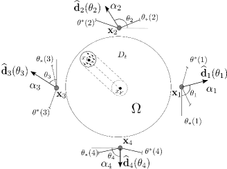
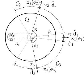
Figure 2: Dipole configuration and two different moving subdomains $D_{t}$ within $\Omega\subset\mathbb{R}^{2}$. These domains, $D_{1,t}$ (left) and $D_{2,t}$ (right), do not deform, are initialized at $\bm{x}_{I}$ and travel to their destinations $\bm{x}_{F}$ along different curves. The target vector fields $\left\{\mathbf{f}_{i}\right\}_{i=1}^{2}$, which are tangent to the curve $\mathcal{C}$, are represented by arrows for the initial configuration.

For each of these configurations we have solved the discrete problems with $N=100$ time intervals and $\lambda=\eta=10^{-5}$. In order to solve (4.4), we consider an admissible set characterized by initial conditions ${\bm{\alpha}}_{0}=(2,0,0,2),{\bm{\theta}}_{0}=(0,\pi/2,3\pi/2,3\pi/2)\in\mathbb{R}^{4}$, and by upper and lower bounds for the intensities and angles given by: ${\bm{\alpha}}^{*}=(2,\ldots,2),{\bm{\alpha}}_{*}=(-2,\ldots,-2),{\bm{\theta}}^{*}=(2\pi,\ldots,2\pi),{\bm{\theta}}_{*}=(0,\ldots,0)\in\mathbb{R}^{4}$, respectively. The initial guesses $({\bm{\alpha}}_{int},{\bm{\theta}}_{int})$ are computed by Algorithm 1 with $\verb"tol"=10^{-3}$ with a total of 525 iterations. Notice that, at each time step $n$, the iterations of the minimization problem in Algorithm 1 depends on $n_{p}$ unknowns. We recall that, due to the non-convexity of the cost functional $\mathcal{J}$ (and $\mathcal{J}_{\tau}$), we may converge to different local minima depending on the choice of the initial guess.

The solution $\bar{{\bm{\alpha}}}_{\tau}(t)=(\bar{\alpha}_{i,\tau}(t))_{i=1}^{4},\bar{{\bm{\theta}}}_{\tau}(t)=(\bar{\theta}_{i,\tau}(t))_{i=1}^{4}$ of problem (4.4) with initial guesses given by $({\bm{\alpha}}_{int},{\bm{\theta}}_{int})$ is depicted in Figure 3.

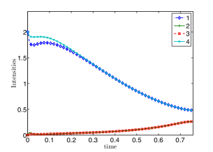
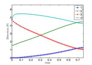
Figure 3: Optimal solution $(\bar{{\bm{\alpha}}}_{\tau},\bar{{\bm{\theta}}}_{\tau})=(\bar{\alpha}_{i,\tau},\bar{\theta}_{i,\tau})_{i=1}^{4}$ to problem (4.4). The evolution of the intensities (left) and direction, characterized by the angle $\theta$(right) are shown for each dipole $i=1,\ldots,4$.

From Figure 3 (left) we observe that the optimal intensity ${\bm{\alpha}}_{i}$ due to $i^{th}$ dipole, is smaller when $D_{t}$ is close to the $i^{th}$ dipole and $\mathbf{f}$ is pointing in a direction opposite to the dipole position. This is due to the fact that the magnetic forces on the boundary of the domain $\Omega$ are much higher than inside $\Omega$, thus making it difficult to approximate the magnetic force when $D_{t}$ is close to the boundary. In particular, it can be seen that the intensities of dipole 2 and 3 are small when $t$ is close to 0. Such a behavior is expected because $D_{1,t}$ is close to the boundary of $\Omega$, where the magnetic field generated by these dipoles is large, thus it is difficult for dipoles 2 and 3 to “push” in the $\mathbf{f}_{1}$ direction. We also notice that dipoles 1 and 4, which can create an attractive field in the $\mathbf{f}_{1}$ direction, have the largest intensities at initial times and decrease when the time is close to $0.75$. Figure 3 (right) shows the dynamics of the angles $(\bar{\theta}_{i,\tau}(t))_{i=1}^{4}$.

Figure 4 shows the approximate field and dipole configuration for three time instances $t=0.007,0.375,0.75$. Here, the magnitude of magnetic force $|\nabla|{\bm{h}}|^{2}|$ in logarithmic scale (in the background) and the magnetic force represented by arrows are depicted. The bottom figures show the dipoles direction represented by the arrows outside the domain $\Omega$. The top figures illustrate the normalized magnetic force in $\Omega$, but in the bottom figures the force is restricted to $D_{t}$. It can be seen that the magnetic force is close (i.e., almost constant) to $\mathbf{f}_{1}$ in $D_{1,t}$ as expected whereas it is quite far from constant in the entire domain.

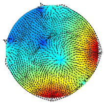
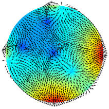
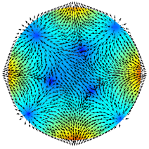
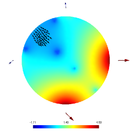
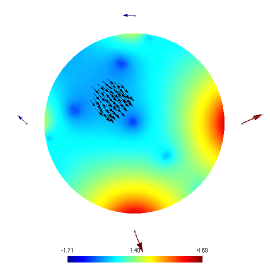
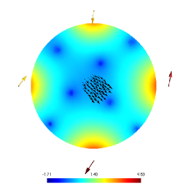
Figure 4: Magnetic force solution to the minimization problem (4.4) with $D_{1,t}$ and vector field $\mathbf{f}_{1}$ (force fields shown by black arrows). Top figure shows the normalized force at three different times $t=0.007,0.375$ and $0.75$ from left to right, respectively. In the bottom figure the magnetic forces are shown only on $D_{1,t}$ for the same time instances. The arrows outside $\Omega$ represent the dipoles with fixed position and variable direction. The magnetic force magnitude $|\nabla|{\bm{h}}|^{2}|$ is shown by the background coloring on a logarithmic scale.

Next, we approximate the vector field $\mathbf{f}_{2}$ defined on $D_{2,t}$. Here, given that we want to create a uniform field $\mathbf{f}_{2}(\bm{x},t)=(1,0)^{\top}$ on a domain which moves from left to the center of $\Omega$ (see Figure 2 (right)), we restrict the position of the dipoles to the right of the domain. Namely, we assume that each dipole $i$ moves along a prescribed trajectory $\mathcal{C}_{i}=1.2[\cos(\phi_{i}),\sin(\phi_{i})],i=1,2,3$, where $\phi_{1}(t)\in(-\pi/90,\pi/90)$, $\phi_{2}(t)\in(\pi/90,3\pi/4)$ and $\phi_{3}(t)\in(-3\pi/4,-\pi/90)$. We solve (4.10) for an admissible set characterized by initial conditions ${\bm{\alpha}}_{0}=(-2,0,0),{\bm{\phi}}_{0}=(0,2\pi/3,4\pi/3)\in\mathbb{R}^{3}$, and by upper and lower bounds for the intensities and angles given by: ${\bm{\alpha}}^{*}=(2,2,2),{\bm{\alpha}}_{*}=(-2,-2,-2),{\bm{\phi}}^{*}=(\pi/90,3\pi/4,2\pi),{\bm{\theta}}_{*}=(-\pi/90,\pi/90,5\pi/4)\in\mathbb{R}^{3}$, respectively.

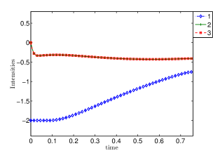
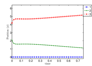
Figure 5: Optimal solution $(\bar{{\bm{\alpha}}}_{\tau},\bar{{\bm{\phi}}}_{\tau})=(\bar{\alpha}_{i,\tau},\bar{\phi}_{i,\tau})_{i=1}^{3}$ to problem (4.10). The evolution of the intensities (left) and position, characterized by the angle $\phi$, (right) are shown for each dipole $i=1,\ldots,3$.

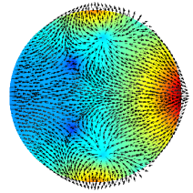
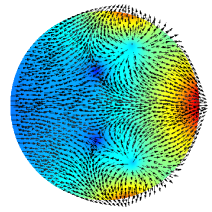
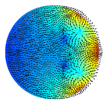
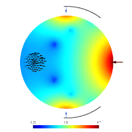
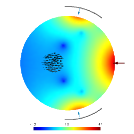
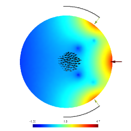
Figure 6: Magnetic force solution to the minimization problem (4.10) with $D_{2,t}$ and vector field $\mathbf{f}_{2}$ (force fields shown by black arrows). Top figures shows the normalized force at three different times $t=0.007,0.375$ and $0.75$ from left to right, respectively. In the bottom figures the magnetic forces is defined only on $D_{2,t}$ for the same time instances. The arrows outside $\Omega$ represent the dipoles with fixed direction and variable position. The path covered by each dipole is depicted by the line outside $\Omega$. The magnetic force magnitude $|\nabla|{\bm{h}}|^{2}|$ is shown by the background coloring on a logarithmic scale.

The vector intensities $(\bar{\alpha}_{i,\tau})_{i=1}^{3}$ and the parametrization of the position $(\bar{\phi}_{i,\tau})_{i=1}^{3}$ solutions to the minimization problem (4.10) are shown in Figure 5 left and right, respectively . We notice that the first dipole attains a fixed position and intensity (the maximum intensity), whereas dipoles 2 and 3 are moving but their intensity is almost constant. Given that we want to approximate a uniform and unitary vector field on $D_{1,t}$, the intensity of dipole 1 decreases as the domain approaches dipole 1. This is due to the fact that the force applied to the edge of $D_{1,t}$, close to dipole 1, is larger than the one applied to the farther edge, and this difference increases as $D_{1,t}$ is close to the source.

The magnetic force and dipole positions are shown for three time instances $t=0.007,0.375$ and $0.75$ in Figures 6. Here dipoles 2 and 3 “follows” the trajectory of $D_{2,t}$ which allows to obtain an almost constant field on the moving domain. From the previous figures it can be seen that our proposed minimization procedure produces a vector field that is close to the target field.

6 Numerical solution of the convection-dominated diffusion equation

From the previous section it follows that an almost uniform magnetic force field can be attained in a small region for two different dipole configurations. In this section we move a concentration of ferrofluid modeled by (1.1)-(1.3) where the advection term is computed either by solving the minimization problem (3.1) or (3.3) depending on the dipole configuration. The aim of these examples is to study the feasibility of the dipole configurations to create a magnetic force that allow us to “push” the concentration inside the domain.

For simplicity, we assume $\gamma=\nu=1$, ${\bm{u}}={\bm{0}}$. To further minimize the spreading we choose a small diffusion coefficient, in particular, we set $A=\varepsilon\mathbb{I}$, with $\varepsilon\ll 1$. As a result the advection diffusion equation (1.1) and (1.2) can be written as

$$\partial_{t}c+\mathop{\mathrm{div}}\nolimits\left(-\varepsilon\nabla c+c\nabla|{\bm{h}}|^{2}\right)=0\quad\mbox{in }\widetilde{\Omega}\times(0,T)$$ (6.1a)

$$(-\varepsilon\nabla c+c\nabla|{\bm{h}}|^{2})\cdot\bm{n}=0\quad\mbox{on }\partial\widetilde{\Omega}\times(0,T)\qquad c(x,0)=c_{0}\quad\mbox{in }\widetilde{\Omega}$$ (6.1b)

Multiplying (6.1a) by a test function $v\in\mathrm{H}^{1}(\widetilde{\Omega})$, integrating by parts, and using the boundary condition in (6.1b) leads us to the following problem: Given $c_{0}\in\mathrm{L}^{2}(\widetilde{\Omega})$, find $c\in\mathrm{L}^{2}(0,T;\mathrm{H}^{1}(\widetilde{\Omega}))\cap\mathrm{H}^{1}(0,T;\mathrm{H}^{1}(\widetilde{\Omega})^{\prime})$ such that

$$\langle\partial_{t}c,v\rangle+\left(\varepsilon\nabla c-c\nabla|{\bm{h}}|^{2},\nabla v\right) =0\quad\forall v\in\mathrm{H}^{1}(\widetilde{\Omega}),$$ (6.2a)

$$c(x,0) =c_{0}\quad\mbox{in }\widetilde{\Omega},$$ (6.2b)

here $\langle\cdot,\cdot\rangle$ is the duality product between $\mathrm{H}^{1}(\widetilde{\Omega})$ and $\mathrm{H}^{1}(\widetilde{\Omega})^{\prime}$. The existence and uniqueness of solution to this problems follows, for instance, from [11, Theorem 6.6]. Notice that in case of the Dirichlet boundary condition $c=0$ we must replace $\mathrm{H}^{1}(\widetilde{\Omega})$ by $\mathrm{H}^{1}_{0}(\widetilde{\Omega})$ in the above calculations.

Below we present two numerical examples. In the first example we consider a simplified $\widetilde{\Omega}$ whose size is comparable to $\Omega$ where the goal is to magnetically inject the concentration of nanoparticles. With the current configuration, the concentration may reach the boundary and, as is mentioned in [25] for a similar problem, boundary layers may appear. On the other hand, given that we are interested in the case $\varepsilon\ll 1$, a proper space discretization has to be considered in order to avoid numerical oscillations. We adopt a monotone scheme for space discretization: edge-averaged finite element (EAFE) [30]. Other alternatives such as SUPG stabilization are equally valid. Given that the EAFE scheme is a type of upwinding scheme, we observe a significant diffusion in all cases. Thus making it difficult to control the concentration in case of complicated geometries, for instance the flow around an obstacle.

As a second example we study the feasibility of moving the concentration around an obstacle. In order to ensure the uniformity of the field we consider a small, but complex, domain $\widetilde{\Omega}$ (see Figure 7 (right)). Moreover, it is shown that Dirichlet boundary condition $c=0$ on $\partial\widetilde{\Omega}$ in (6.1b) is meaningful in this example. For the numerical approximation we consider piecewise linear finite element space discretization and explicit Euler scheme for time discretization. In order to avoid having to solve a linear system at each time step we consider mass lumping with a correction technique to account for the dispersive effects (see [15]). In section 6.1 we discuss the EAFE scheme and in section 6.2 we discuss the explicit scheme. Numerical examples are presented in each case.

6.1 Edge-averaged Finite Element (EAFE) Method and Magnetic Injection

It is well–known that the standard finite element method applied to problem (6.2), yields solution oscillations when $\varepsilon\ll\|\nabla|{\bm{h}}|^{2}\|_{L^{\infty}(0,T;\widetilde{\Omega})}$. However, there is no universal approach to treat such problems. In order to choose a numerical scheme to approximate problem (6.2) first notice an interesting feature of the flux $J(c)$ of (6.1a):

$$J(c)\mathrel{\mathop{\mathchar 58\relax}}=\varepsilon\nabla c-\nabla|{\bm{h}}|^{2}c=e^{|{\bm{h}}|^{2}\varepsilon^{-1}}\nabla\left(\varepsilon\,e^{-|{\bm{h}}|^{2}\varepsilon^{-1}}c\right)=a\nabla u$$ (6.3)

i.e., it is symmetrizable. Here

$$a=e^{|{\bm{h}}|^{2}\varepsilon^{-1}},\quad\psi=-|{\bm{h}}|^{2}\varepsilon^{-1},\quad u=\varepsilon e^{\psi}c.$$ (6.4)

Equations with the above property have been studied by many authors (see, for instance, [6, 24]). They also appear in applications such as semiconductors device simulation. In order to exploit the structure of the equation, for the numerical approximation we consider the edge-average finite element (EAFE), a monotone scheme introduced in [30] for stationary advection-diffusion equations. It was later extended to time-dependent advection-diffusion equations in [3] and compared with SUPG, another well-known stabilization technique. With this in mind we adapt the scheme presented in [3] to our particular case.

We begin by recalling the EAFE scheme of [30] and apply it to the symmetric operator in (6.3). We denote by $\mathcal{T}_{h}$ a shape regular triangulation of $\widetilde{\Omega}$ and by $\mathrm{H}_{h}\subset\mathrm{H}^{1}(\Omega)$ the space of piecewise linear finite elements with hat basis $\{\phi_{i}\}_{i=1}^{N}$. Notice that the scheme proposed below is equally applicable to both the Neumann and the Dirichlet problems. We designate by $E=E_{ij}$ the edge connecting the nodes $x_{i}$ and $x_{j}$. The discrete weak form of $-\textrm{div }(a\nabla u)$ reads

$$\int_{\Omega}a\nabla u_{h}\cdot\nabla v_{h}=\sum_{T\in\mathcal{T}_{h}}\int_{\Omega}a\nabla u_{h}\cdot\nabla v_{h}=-\sum_{T\in\mathcal{T}_{h}}\sum_{E\subset\partial T}a_{E}^{T}\delta_{E}(e^{\psi}c_{h})\delta_{E}v_{h},$$ (6.5)

where $\delta_{E}(w_{h})=w_{i}-w_{j}$ and

$$a_{E}^{T}=\left(\ \int_{T}\varepsilon a\nabla\phi_{i}\cdot\nabla\phi_{j}\,dx\right)=\left(\frac{1}{|T|}\int_{T}\varepsilon e^{-\psi}\,dx\right)\left(\int_{T}\nabla\phi_{i}\cdot\nabla\phi_{j}\,dx\right)$$

because $\nabla\phi_{i}$ is piecewise constant. We now replace the first factor by the so-called harmonic average over the edge $E$, namely

$$\alpha_{E}\mathrel{\mathop{\mathchar 58\relax}}=\left(\frac{1}{|E|}\int_{E}\varepsilon^{-1}e^{\psi}\,dx\right)^{-1}\approx\frac{1}{|T|}\int_{T}\varepsilon e^{-\psi}\,dx.$$

Upon setting $\omega_{E}^{T}\mathrel{\mathop{\mathchar 58\relax}}=\int_{T}\nabla\phi_{i}\cdot\nabla\phi_{j}$, we realize that (6.5) can be approximated by

$$\mathcal{B}_{h}(c_{h},v_{h})\mathrel{\mathop{\mathchar 58\relax}}=-\sum_{T\in\mathcal{T}_{h}}\left(\sum_{E\subset\partial T}\omega_{E}^{T}\alpha_{E}\delta_{E}(e^{\psi}c_{h})\delta_{E}(v_{h})\right)\quad\forall\,c_{h},v_{h}\in\mathrm{H}_{h},$$ (6.6)

which is the bilinear form corresponding to the EAFE scheme of [30].

For the time interval $[0,T]$ we introduce a uniform partition $0=t_{0}<t_{1}<\ldots<t_{N}=T$, with $N\geq 1$, and denote by $\Delta t=T/N$ the time step size. By applying the implicit Euler scheme for time discretization, we obtain the following fully discrete scheme of problem $\eqref{eq:weak}$: Given $c_{0}\in\mathrm{L}^{2}(\widetilde{\Omega})$, for $n=1,\ldots,N$ find $c^{n}_{h}\in\mathrm{H}_{h}$ such that

$$(c^{n}_{h},v_{h})+\Delta t\mathcal{B}_{h}(c^{n}_{h},v_{h}) =(c^{n-1}_{h},v_{h})\quad\forall v_{h}\in\mathrm{H}_{h}$$ (6.7a)

$$c^{0}_{h} =c_{0}$$ (6.7b)

Error estimates of a similar discrete problem can be found in [3].

In the following subsections we will study the feasibility of the manipulation of nanoparticles concentration by controlling the dipole intensity and direction. To fix ideas, let $\Omega$ be a ball of unit radius centered at $(0,0)$. The configuration of the 4 dipoles is same as in the previous example (cf. Section 5.1).

In our first example we focus on magnetically injecting the initial concentration $c_{0}$ of nanoparticles so that it arrives at a desired location. Instead of just the intensity (cf. [2, 20]) the control variables here are both the intensities and the directions of the dipoles. Additionally, the concentration is close to the boundary for certain time instances. A standard Galerkin scheme in space usually leads to oscillations in this case. We assume that the domain $\widetilde{\Omega}\subset\Omega$ is a $\pi/4$ clockwise rotation of the rectangle $[-0.9,0.9]\times[-0.3,0.3]$ (cf. Figure 7, left). We set the final time $T=0.75$ and $c_{0}(x,y)=\exp\left(3\times 10^{-5}((x+0.53)^{2}+(y-0.53)^{2})\right)$ (cf. Figures 7 and 8 (left)).

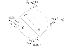
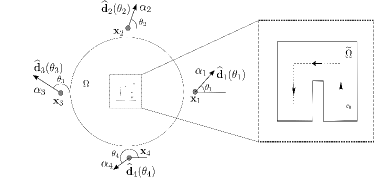
Figure 7: Computational domain $\widetilde{\Omega}\subset\Omega$ and dipole configuration with fixed position and variable direction and intensity.

We use the optimal magnetic force computed in the first example of Section 5.1 (cf.  Figure 4) as an input to (6.7). Here we have set $\varepsilon=10^{-5}$, $\Delta t=7.5\times 10^{-3}$ and $h=0.0065$. The initial concentration is located at $(-0.53,0.53)$ and the final location is $(0,0)$, see Figure 7 (left). Figure 8 shows the snapshots of concentration at three time instances.

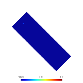
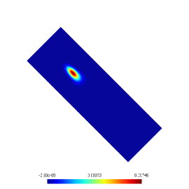
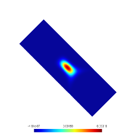
Figure 8: Evolution of the concentration in $\widetilde{\Omega}$ at times $t=0,0.375,0.75$ with $\varepsilon=10^{-5}$

Notice that (cf. Figure 8) the concentration reaches the desired location. Since we are using 4 dipoles instead of 8 dipoles used in (cf. [2, 20]) we find it difficult to control the diffusion, also notice that we have Neumann boundary conditions here. Indeed the spikes in Figure 8 (right) can be explained by the behavior of the magnetic force given in Figures 3 (left) and 4 (right).

6.2 Explicit Scheme and Magnetic Injection Around an Obstacle

Our next example explores the possibility of moving the concentration around an obstacle. Indeed a larger $\varepsilon$ leads to significant diffusion and it is not possible to accomplish our goal. On the other hand, a smaller $\varepsilon$ can computationally lead to an ill-posed problem; recall the Neumann boundary condition:

$$(-\varepsilon\nabla c+c\nabla|{\bm{h}}|^{2})\cdot\bm{n}=0\quad\mbox{on }\partial\widetilde{\Omega}\times(0,T).$$

So when $\varepsilon$ is small then an appropriate boundary condition is Dirichlet (assuming that $\nabla|{\bm{h}}|^{2}\cdot\bm{n}\neq 0$).

Motivated by this, we consider the advection-diffusion equation (6.1a) but with the Dirichlet boundary condition $c=0$ on $\partial\widetilde{\Omega}\times(0,T)$. The latter is also physically meaningful if the concentration stays away from the boundary at all times. Even for small parameter $\varepsilon$ we observe a relatively large diffusion both in case of EAFE scheme and stabilized implicit (in time) scheme [2]. For that reason and, in order to ensure that the concentration is far from the boundary, we have adopted a piecewise linear finite element scheme for the space approximation and the explicit Euler scheme for the time discretization.

The fully discrete problem is: Given $c_{0}\in\mathrm{L}^{2}(\widetilde{\Omega})$, for $n=1,\ldots,N$ find $c^{n}_{h}\in\mathrm{H}_{h,0}\subset\mathrm{H}_{0}^{1}(\widetilde{\Omega})$ such that

$$(c^{n}_{h},v_{h}) =(c^{n-1}_{h},v_{h})-\Delta ta(c^{n-1}_{h},v_{h})\quad\forall v_{h}\in\mathrm{H}_{h,0}$$ (6.8a)

$$(c^{0}_{h},\phi) =(c_{0},\phi)\quad\forall\phi\in\mathrm{H}_{h,0},$$ (6.8b)

with $a(c^{n-1}_{h},v_{h})=\int_{\Omega}\varepsilon\nabla c_{h}^{n-1}\cdot\nabla v_{h}-c_{h}^{n-1}\nabla|{\bm{h}}|^{2}\cdot\nabla v_{h}\;dx$.

In the matrix vector notation the system in (6.8) is given by

$${\bm{M}}{\bm{c}}^{n} ={\bm{M}}{\bm{c}}^{n-1}-\Delta t{\bm{A}}{\bm{c}}^{n-1}$$ (6.9a)

$${\bm{M}}{\bm{c}}^{0} ={\bm{M}}{\bm{c}}_{0},$$ (6.9b)

where ${\bm{M}}=(m_{ij})_{i,j}$ with $m_{ij}=\int_{\Omega}\phi_{i}\phi_{j}$ and ${\bm{A}}$ are the mass and the stiffness matrices, respectively. Moreover, for every $k\in\{1,\dots,N\}$ the vector ${\bm{c}}^{k}$ contains the finite element nodal values. Clearly (6.9) requires solving a linear system at every time. To avoid such a linear solve we employ the mass lumping (with correction) of [15]. Let $\overline{\bm{M}}=(\overline{m}_{ij})_{i,j}$ denotes a diagonal lumped mass matrix with diagonal entries given by $\overline{m}_{ii}=\sum_{j}m_{ij}$. Then we approximate ${\bm{M}}^{-1}$ by replacing the inverse of the lumped mass matrix by $(\mathbb{I}+{\bm{B}}_{r})\overline{\bm{M}}^{-1}$ where ${\bm{B}}_{r}=\overline{\bm{M}}^{-1}(\overline{\bm{M}}-{\bm{M}})$.

Our domain of interest is $\widetilde{\Omega}=[-0.18,0.18]^{2}\setminus[-0.02,0.02]\times[-0.18,0]$ depicted on Figure 7 (right) where the path traversed by the concentration is given by the dotted line. Our aim is to move the initial concentration

$$c_{0}(x,y)=\exp\left(10^{-4}((x-0.1)^{2}+(y+0.1)^{2})\right)$$

from the initial location $(0.1,-0.1)$ at $t=0$ to the final location $(-0.1,-0.1)$ at $t=T=0.6$. With this in mind, we first solve the optimal control problem (4.4) with a ball of radius $0.2$ centered at $(0.1,-0.1)$ as a reference domain $\widehat{D}$. We approximate a time dependent vector field given by $\mathbf{f}(\bm{x},t)$ such that: $\mathbf{f}(\bm{x},t)=(0,1)^{\top}$ if $0\leq t<0.2$, $\mathbf{f}(\bm{x},t)=(-1,0)^{\top}$ if $0.2\leq t<0.4$ and $\mathbf{f}(\bm{x},t)=(0,-1)^{\top}$ if $0.4\leq t\leq 0.6$. The moving domains $D_{t}$ is such that $D_{t}=\bm{x}_{I}(t,\widehat{D})$, with $\bm{x}_{I}(t,\widehat{\bm{x}})=\bm{\varphi}(t)+\widehat{\bm{x}}$. Here $\bm{\varphi}(t)$, which represents the trajectory of the barycenter of $D_{t}$, is defined as: $\bm{\varphi}(t)=(0.1,-0.1)+t(0,1)^{\top}$ if $0\leq t<0.2$, $\bm{\varphi}(t)=(0.1,0.1)+(t-0.2)(-1,0)^{\top}$ if $0.2\leq t<0.4$ and $\bm{\varphi}(t)=(-0.1,0.1)+(t-0.4)(0,-1)^{\top}$ if $0.4\leq t\leq 0.6$. Figure 9 (top row) shows the resulting magnetic force at four different times.

In order to steer $c_{0}$ around the obstacle shown in Figure 9, we use the above optimal force as input to (6.8). The bottom row in Figure 9 shows the concentration snapshots at four different times. Here we have set $\varepsilon=10^{-8}$, $\Delta t=3\times 10^{-5}$ and mesh size $h=0.0016$.

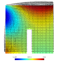
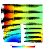
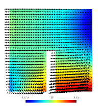
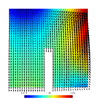
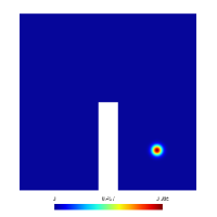
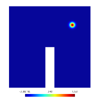
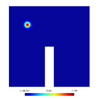
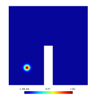
Figure 9: Top figures: optimal magnetic force computed by solving (4.4). The magnitude the magnetic force is shown by the background color. Bottom figures: Evolution of the concentration in $\widetilde{\Omega}$ when the optimal magnetic force is used as an input to (6.8). The columns correspond to $t=0,0.2,0.4$ and $0.6$ from left to right, respectively.

The top row in Figure 9 shows the optimal magnetic force obtained by solving (4.4). The bottom row shows the evolution of the concentration at four different time instances. Notice that the magnetic forces prevent the concentration from reaching the boundary $\partial\widetilde{\Omega}$ and enables the concentration to reach the final location at $(-0.1,0.1)$ while avoiding the obstacle.

References

- [1] H. Antil, M. Hintermueller, R. H. Nochetto, T. M. Surowiec, and D. Wegner. Finite horizon model predictive control of electrowetting on dielectric with pinning. 2017. (accepted).
- [2] H. Antil, R.H. Nochetto, and P. Venegas. Optimal control of kelvin force in a bounded domain. 2016. (submitted) http://arxiv.org/abs/1612.07763.
- [3] N.R. Bayramov and J.K. Kraus. On the stable solution of transient convection–diffusion equations. Journal of Computational and Applied Mathematics, 280:275 – 293, 2015.
- [4] A. Braides. Local minimization, variational evolution and -convergence, volume 2094 of Lecture Notes in Mathematics. Springer, Cham, 2014.
- [5] H. Brezis. Functional Analysis, Sobolev Spaces and Partial Differential Equations. Springer, 2011.
- [6] F. Brezzi, L. D. Marini, and P. Pietra. Two-dimensional exponential fitting and applications to drift-diffusion models. SIAM Journal on Numerical Analysis, 26(6):1342–1355, 1989.
- [7] H. Choi, M. Hinze, and K. Kunisch. Instantaneous control of backward-facing step flows. Appl. Numer. Math., 31(2):133–158, 1999.
- [8] H. Choi, R. Temam, P. Moin, and J. Kim. Feedback control for unsteady flow and its application to the stochastic Burgers equation. J. Fluid Mech., 253:509–543, 1993.
- [9] G. Dal Maso. An introduction to -convergence. Progress in Nonlinear Differential Equations and their Applications, 8. Birkhäuser Boston, Inc., Boston, MA, 1993.
- [10] J. Dobson. Gene therapy progress and prospects: Magnetic nanoparticle-based gene delivery. Gene Ther, 13:283–287, 2006.
- [11] A. Ern and J.-L. Guermond. Theory and Practice of Finite Elements, volume 159 of Applied Mathematical Sciences. Springer–Verlag, New York, 2004.
- [12] T.W.R. Fountain, P.V. Kailat, and J.J. Abbott. Wireless control of magnetic helical microrobots using a rotating-permanent-magnet manipulator. In Robotics and Automation (ICRA), 2010 IEEE International Conference on, pages 576–581, 2010.
- [13] M.A.M. Gijs, F. Lacharme, and U. Lehmann. Microfluidic applications of magnetic particles for biological analysis and catalysis. Chem. Rev., 110(3):1518–1563, 2010.
- [14] A. D. Grief and G. Richardson. Mathematical modelling of magnetically targeted drug delivery. Journal of Magnetism and Magnetic Materials, 293:455 – 463, 2005. Proceedings of the Fifth International Conference on Scientific and Clinical Apllications of Magnetic Carriers.
- [15] Jean-Luc Guermond and Richard Pasquetti. A correction technique for the dispersive effects of mass lumping for transport problems. Computer Methods in Applied Mechanics and Engineering, 253:186 – 198, 2013.
- [16] M. Hintermüller, K. Ito, and K. Kunisch. The primal-dual active set strategy as a semismooth newton method. SIAM J. on Optimization, 13(3):865–888, August 2002.
- [17] M. Hinze and A. Kauffmann. On a distributed control law with an application to the control of unsteady flow around a cylinder. In Optimal Control of Partial Differential Equations, volume 133 of ISNM International Series of Numerical Mathematics, pages 177–190. Birkhäuser Basel, 1999.
- [18] B. G. Hosu, K. Jakab, P. Bánki, F. I. Tóth, and G. Forgacs. Magnetic tweezers for intracellular applications. Review of Scientific Instruments, 74(9):4158–4163, 2003.
- [19] C. T. Kelley. Iterative methods for optimization. Number 18 in Frontiers in Applied Mathematics. SIAM, 1999.
- [20] A. Komaee and B. Shapiro. Magnetic steering of a distributed ferrofluid spot towards a deep target with minimal spreading. In Decision and Control and European Control Conference (CDC-ECC), 2011 50th IEEE Conference on, pages 7950–7955, Dec 2011.
- [21] J.K. Lim, S. P. Yeap, and S. C. Low. Challenges associated to magnetic separation of nanomaterials at low field gradient. Separation and Purification Technology, 123:171 – 174, 2014.
- [22] AS. Lübbe, C. Bergemann, H. Riess, F. Schriever, P. Reichardt, K. Possinger, M. Matthias, B. Dörken, F. Herrmann, and R. Gürtler. Clinical experiences with magnetic drug targeting: A phase I study with 4’-Epidoxorubicin in 14 patients with advanced solid tumors. Cancer Research, 56(20):4686–4693, 1996.
- [23] A. W. Mahoney and J.J. Abbott. Managing magnetic force applied to a magnetic device by a rotating dipole field. Applied Physics Letters, 99, 2011.
- [24] P. A. Markowich and M. A. Zlámal. Inverse-average-type finite element discretizations of selfadjoint second-order elliptic problems. Mathematics of Computation, 51(184):431–449, 1988.
- [25] A. Nacev, C. Beni, O. Bruno, and B. Shapiro. The behaviors of ferro-magnetic nano-particles in and around blood vessels under applied magnetic fields. Journal of magnetism and magnetic materials, 323(6):651–668, 2011.
- [26] B. J. Nelson, I. K. Kaliakatsos, and J.J. Abbott. Microrobots for minimally invasive medicine. Annual Review of Biomedical Engineering, 12:55–85, 2010.
- [27] A.J. Petruska and J.J. Abbott. Optimal permanent-magnet geometries for dipole field approximation. Magnetics, IEEE Transactions on, 49:811–819, 2013.
- [28] A. Solanki, J. D. Kim, and K.-B. Lee. Nanotechnology for regenerative medicine: nanomaterials for stem cell imaging. Nanomedicine, 3(4):567–578, 2008.
- [29] F. Tröltzsch. Optimal Control of Partial Differential Equations: Theory, Methods and Applications. Grad. Stud. Math. 112, AMS, Providence, 2010.
- [30] J. Xu and L. Zikatanov. A monotone finite element scheme for convection-diffusion equations. Mathematics of Computation, 68(228):1429–1446, 1999.