Algorithms for Covering Multiple Barriers

Abstract

In this paper, we consider the problems for covering multiple intervals on a line. Given a set $B$ of $m$ line segments (called “barriers”) on a horizontal line $L$ and another set $S$ of $n$ horizontal line segments of the same length in the plane, we want to move all segments of $S$ to $L$ so that their union covers all barriers and the maximum movement of all segments of $S$ is minimized. Previously, an $O(n^{3}\log n)$-time algorithm was given for the case $m=1$. In this paper, we propose an $O(n^{2}\log n\log\log n+nm\log m)$-time algorithm for a more general setting with any $m\geq 1$, which also improves the previous work when $m=1$. We then consider a line-constrained version of the problem in which the segments of $S$ are all initially on the line $L$. Previously, an $O(n\log n)$-time algorithm was known for the case $m=1$. We present an algorithm of $O(m\log m+n\log m\log n)$ time for any $m\geq 1$. These problems may have applications in mobile sensor barrier coverage in wireless sensor networks.

arrier coverage, geometric coverage, mobile sensors, algorithms, data structures, computational geometry

1 Introduction

In this paper, we study algorithms for the problems for covering multiple barriers. These are basic geometric problems and may have applications in barrier coverage of mobile sensors in wireless sensor networks. For convenience, in the following we introduce and discuss the problems from the mobile sensor barrier coverage point of view.

Let $L$ be a line, say, the $x$-axis. Let $\mathcal{B}$ be a set of $m$ pairwise disjoint segments, called barriers, sorted on $L$ from left to right. Let $S$ be a set of $n$ sensors in the plane, and each sensor $s_{i}\in S$ is represented by a point with coordinate $(x_{i},y_{i})$. If a sensor is moved on $L$, it has a sensing/covering range of length $r$, i.e., if a sensor $s$ is located at $x$ on $L$, then all points of $L$ in the interval $[x-r,x+r]$ are covered by $s$ and the interval is called the covering interval of $s$. The problem is to move all sensors of $S$ onto $L$ such that each point of every barrier is covered by at least one sensor and the maximum movement of all sensors of $S$ is minimized, i.e., the value $\max_{s_{i}\in S}\sqrt{(x_{i}-x_{i}^{\prime})^{2}+y_{i}^{2}}$ is minimized, where $x_{i}^{\prime}$ is the location of $s_{i}$ on $L$ in the solution (its $y$-coordinate is $0$ since $L$ is the $x$-axis). We call it the multiple-barrier coverage problem, denoted by MBC.

We assume that covering range of the sensors is long enough so that a coverage of all barriers is always possible. Note that we can check whether a coverage is possible in $O(m+n)$ time by an easy greedy algorithm (e.g., try to cover all barriers one by one from left to right using sensors in such a way that their covering intervals do not overlap except at their endpoints).

Previously, the case $m=1$ was studied and the problem was solved in $O(n^{3}\log n)$ time [16]. In this paper, we propose an $O(n^{2}\log n\log\log n+nm\log m)$-time algorithm for any $m\geq 1$, which also improves the algorithm in [16] by almost a linear factor when $m=1$.

We further consider a line-constrained version of the problem where all sensors of $S$ are initially on $L$. Previously, the case $m=1$ was studied and the problem was solved in $O(n\log n)$ time [4]. We present an $O(m\log m+n\log m\log n)$ time algorithm for any $m\geq 1$, and the running time matches that of the algorithm in [4] when $m=1$.

1.1 Related Work

Sensors are basic units in wireless sensor networks. The advantage of allowing the sensors to be mobile increases monitoring capability compared to those static ones. One of the most important applications in mobile wireless sensor networks is to monitor a barrier to detect intruders in an attempt to cross a specific region. Barrier coverage [14, 16], which guarantees that every movement crossing a barrier of sensors will be detected, is known to be an appropriate model of coverage for such applications. Mobile sensors normally have limited battery power and therefore their movements should be as small as possible.

Dobrev et al. [9] studies several problems on covering multiple barriers in the plane. They showed that these problems are generally NP-hard when sensors have different ranges. They also proposed polynomial-time algorithms for several special cases of the problems, e.g., barriers are parallel or perpendicular to each other, and sensors have some constrained movements. In fact, if sensors have different ranges, by an easy reduction from the Partition Problem as in [9], we can show that our problem MBC is NP-hard even for the line-constrained version and $m=2$.

Other previous work has been focused on the line-constrained problem with $m=1$. Czyzowicz et al. [7] first gave an $O(n^{2})$ time algorithm, and later, Chen et al. [4] solved the problem in $O(n\log n)$ time. If sensors have different ranges, Chen et al. [4] presented an $O(n^{2}\log n)$ time algorithm. For the weighted case where sensors have weights such that the moving cost of a sensor is its moving distance times its weight, Lee et al. [15] gave an $O(n^{2}\log n\log\log n)$ time algorithm for the case where sensors have the same range.

The min-sum version of the line-constrained problem with $m=1$ has also been studied, where the objective is to minimize the sum of the moving distances of all sensors. If sensors have different ranges, then the problem is NP-hard [8]. Otherwise, Czyzowicz et al. [8] gave an $O(n^{2})$ time algorithm, and Andrews and Wang [1] improved the algorithm to $O(n\log n)$ time. The min-num version of the problem was also studied, where the goal is to move the minimum number of sensors to form a barrier coverage. Mehrandish et al. [18, 19] proved that the problem is NP-hard if sensors have different ranges and gave polynomial time algorithms otherwise.

Bhattacharya et al. [3] studied a circular barrier coverage problem in which the barrier is a circle and the sensors are initially located inside the circle. The goal is to move sensors to the circle to form a regular $n$-gon (so as to cover the circle) such that the maximum sensor movement is minimized. An $O(n^{3.5}\log n)$-time algorithm was given in [3] and later Chen et al. [5] improved the algorithm to $O(n\log^{3}n)$ time. The min-sum version of the problem was also studied [3, 5].

1.2 Our Approach

To solve the problem MBC, one major difficulty is that we do not know the order of the sensors of $S$ on $L$ in an optimal solution. Therefore, our main effort is to find such an order. To this end, we first develop a decision algorithm that can determine whether $\lambda\geq\lambda^{*}$ for any value $\lambda$, where $\lambda^{*}$ is the maximum sensor movement in an optimal solution. Our decision algorithm runs in $O(m+n\log n)$ time. Then, we solve the problem MBC by “parameterizing” the decision algorithm in a way similar in spirit to parametric search [17]. The high-level scheme of our algorithm is very similar to those in [4, 15], but many low-level computations are different.

The line-constrained version of the problem is much easier due to an order preserving property: there exists an optimal solution in which the order of the sensors is the same as in the input. This leads to a linear-time decision algorithm using the greedy strategy. Also based on this property, we can find a set $\Lambda$ of $O(n^{2}m)$ “candidate values” such that $\Lambda$ contains $\lambda^{*}$. To avoid computing $\Lambda$ explicitly, we implicitly organize the elements of $\Lambda$ into $O(n)$ sorted arrays such that each array element can be found in $O(\log m)$ time. Finally, by applying the matrix search technique in [12], along with our linear-time decision algorithm, we compute $\lambda^{*}$ in $O(m\log m+n\log m\log n)$ time. We should point out that implicitly organizing the elements of $\Lambda$ into sorted arrays is the key and also the major difficulty for solving the problem, and our technique may be interesting in its own right.

The rest of the paper is organized as follows. We introduce some notation in Section 2. In Section 3, we present our algorithm for the line-constrained problem. In Section 4, we present our decision algorithm for the problem MBC. Section 5 solves the problem MBC. We conclude the paper in Section 6, with remarks that our techniques can be used to reduce the space complexities of some previous algorithms in [15].

2 Preliminaries

We denote the barriers of $\mathcal{B}$ by $B_{1},B_{2},\ldots,B_{m}$ sorted on $L$ from left to right. For each $B_{i}$, let $a_{i}$ and $b_{i}$ denote the left and right endpoints of $B_{i}$, respectively. For ease of exposition, we make a general position assumption that $a_{i}\neq b_{i}$ for each $B_{i}$. The degenerated case can also be handled by our techniques, but the discussions would be more tedious.

With a little abuse of notation, for any point $x$ on $L$ (the $x$-axis), we also use $x$ to denote its $x$-coordinate, and vice versa. We assume that the left endpoint of $B_{1}$ is at $0$, i.e., $a_{1}=0$. Let $\beta$ denote the right endpoint of $B_{m}$, i.e., $\beta=b_{m}$.

We denote the sensors of $S$ by $s_{1},s_{2},\ldots,s_{n}$ sorted by their $x$-coordinates. For each sensor $s_{i}$ located on a point $x$ of $L$, $x-r$ and $x+r$ are the left and right endpoints of the covering interval of $s_{i}$, respectively, and we call them the left and right extensions of $s_{i}$, respectively.

Again, let $\lambda^{*}$ be the maximum sensor movement in an optimal solution. Given $\lambda$, the decision problem is to determine whether $\lambda\geq\lambda^{*}$, or equivalently, whether we can move each sensor with distance at most $\lambda$ such that all barriers can be covered. If yes, we say that $\lambda$ is a feasible value. Thus, we also call it a feasibility test on $\lambda$.

In the following, we assume that $\lambda^{*}>0$, i.e., we have to move at least one sensor to produce a solution. This can be easily verified in $O((m+n)\log(m+n))$ time by checking whether all barriers can be covered by all sensors in the input.

3 The Line-Constrained Version of MBC

In this section, we present our algorithm for the line-constrained MBC. As in the special case $m=1$ [7], since the sensing ranges of all sensors are equal, a useful observation is that the order preserving property holds: There exists an optimal solution in which the order of the sensors is the same as in the input. Due to this property, we first give a linear-time greedy algorithm for feasibility tests.

Lemma 1

Given any $\lambda>0$, we can determine whether $\lambda$ is a feasible value in $O(n+m)$ time.

Proof

We first move every sensor rightwards for distance $\lambda$. Then, every sensor is allowed to move leftwards at most $2\lambda$ but is not allowed to move rightwards any more. Next we use a greedy strategy to move sensors leftwards as little as possible to cover the currently uncovered leftmost barrier. To this end, we maintain a point $p$ on a barrier that we need to cover such that all barrier points to the left of $p$ are covered but the barrier points to the right of $p$ are not. We consider the sensors $s_{i}$ and the barriers $B_{j}$ from left to right.

Initially, $i=j=1$ and $p=a_{1}$. In general, suppose $p$ is located at a barrier $B_{j}$ and we are currently considering $s_{i}$. If $p$ is at $\beta$, then we are done and $\lambda$ is feasible. If $p$ is located at $b_{j}$ and $j\neq m$, then we move $p$ rightwards to $a_{j+1}$ and proceed with $j=j+1$. In the following, we assume that $p$ is not at $b_{j}$. Let $x_{i}^{r}=x_{i}+\lambda$, i.e., the location of $s_{i}$ after it is initially moved rightwards by $\lambda$.

1. If $x_{i}^{r}+r\leq p$, then we proceed with $i=i+1$.

2. If $x_{i}^{r}-r\leq p<x_{i}^{r}+r$, we move $p$ rightwards to $x_{i}^{r}+r$.

3. If $x_{i}^{r}-2\lambda-r\leq p<x_{i}^{r}-r$, then we move $s_{i}$ leftwards such that the left extension of $s_{i}$ is at $p$, and we then move $p$ to the right extension of $s_{i}$.

4. If $p<x_{i}^{r}-2\lambda-r$, then we stop the algorithm and report that $\lambda$ is not feasible.

Suppose the above moved $p$ rightwards (i.e., in the second and third cases). Then, if $p\geq\beta$, we report that $\lambda$ is feasible. Otherwise, if $p$ is not on a barrier, then we move $p$ rightwards to the left endpoint of the next barrier. In either case, $p$ is now located at a barrier, denoted by $B_{j}$, and we increase $i$ by one. We proceed as above with $B_{j}$ and $s_{i}$. It is easy to see that the algorithm runs in $O(n+m)$ time. ∎

Let $OPT$ be an optimal solution that preserves the order of the sensors. For each $i\in[1,n]$, let $x^{\prime}_{i}$ be the position of $s_{i}$ in $OPT$. We say that a set of $k$ sensors are in attached positions if the union of their covering intervals is a single interval of length equal to $2rk$. The following lemma is an easy extension of a similar observation for the case $m=1$ in [7].

Lemma 2

There exists a sequence of sensors $s_{i},s_{i+1},\ldots,s_{j}$ in attached positions in $OPT$ such that one of the following three cases holds. (a) The sensor $s_{j}$ is moved to the left by distance $\lambda^{*}$ and $x^{\prime}_{i}=a_{k}+r$ for some barrier $B_{k}$ (i.e., the sensors from $s_{i}$ to $s_{j}$ together cover the interval $[a_{k},a_{k}+2r(j-i+1)]$). (b) The sensor $s_{i}$ is moved to the right by $\lambda^{*}$ and $x^{\prime}_{j}=b_{k}-r$ for some barrier $B_{k}$. (c) The sensor $s_{i}$ is moved rightwards by $\lambda^{*}$ and $s_{j}$ is moved leftwards by $\lambda^{*}$.

Cases (a) and (b) are symmetric in the above lemma. Let $\Lambda_{1}$ be the set of all possible distance values introduced by $s_{j}$ in Case (a). Specifically, for any pair $(i,j)$ with $1\leq i\leq j\leq n$ and any barrier $B_{k}$ with $1\leq k\leq m$, define $\lambda(i,j,k)=x_{j}-(a_{k}+2r(j-i)+r)$. Let $\Lambda_{1}$ consist of $\lambda(i,j,k)$ for all such triples $(i,j,k)$. We define $\Lambda_{2}$ symmetrically to be the set of all possible values introduced by $s_{i}$ in Case (b). We define $\Lambda_{3}$ as the set consisting of the values $[x_{j}-x_{i}-2r(j-i)]/2$ for all pairs $(i,j)$ with $1\leq i<j\leq n$. Clearly, $|\Lambda_{3}|=O(n^{2})$ and both $|\Lambda_{1}|$ and $|\Lambda_{2}|$ are $O(mn^{2})$. Let $\Lambda=\Lambda_{1}\cup\Lambda_{2}\cup\Lambda_{3}$.

By Lemma 2, $\lambda^{*}$ is in $\Lambda$, and more specifically, $\lambda^{*}$ is the smallest feasible value of $\Lambda$. Hence, we can first compute $\Lambda$ and then find the smallest feasible value in $\Lambda$ by using the decision algorithm. However, that would take $\Omega(mn^{2})$ time. To reduce the time, we will not compute $\Lambda$ explicitly, but implicitly organize the elements of $\Lambda$ into certain sorted arrays and then apply the matrix search technique proposed in [12], which has been widely used, e.g., [10, 11]. Since we only need to deal with sorted arrays instead of more general matrices, we review the technique with respect to arrays in the following lemma.

Lemma 3

[10, 11] Given a set of $N$ sorted arrays of size at most $M$ each, we can compute the smallest feasible value of these arrays with $O(\log N+\log M)$ feasibility tests and the total time of the algorithm excluding the feasibility tests is $O(\tau\cdot N\cdot\log M)$, where $\tau$ is the time for evaluating each array element (i.e., given the name of an array $A$ and an index $i$ of $A$, we can compute the value of the element $A[i]$ in $O(\tau)$ time).

With Lemma 3, we can compute the smallest feasible values in the three sets $\Lambda_{1}$, $\Lambda_{2}$, and $\Lambda_{3}$, respectively, and then return the smallest one as $\lambda^{*}$. For $\Lambda_{3}$, Chen et al. [4] (see Lemma 14) gave an approach to order in $O(n\log n)$ time the elements of $\Lambda_{3}$ into $O(n)$ sorted arrays of $O(n)$ elements each such that each array element can be evaluated in $O(1)$ time. Consequently, by applying Lemma 3, the smallest feasible value of $\Lambda_{3}$ can be computed in $O((n+m)\log n)$ time.

For $\Lambda_{1}$ and $\Lambda_{2}$, in the case $m=1$, the elements of each set can be easily ordered into $O(n)$ sorted arrays of $O(n)$ elements each [4]. However, in our problem setting, the problem becomes significantly more difficult if we want to obtain a subquadratic-time algorithm. Indeed, this is the main challenge of our method. In what follows, our main effort is to prove the following lemma.

Lemma 4

For the set $\Lambda_{1}$, in $O(m\log m)$ time, we can implicitly form a set $\mathcal{A}$ of $n$ sorted arrays of at most $(n+1)\cdot m^{2}$ elements each such that each array element can be evaluated in $O(\log m)$ time and every element of $\Lambda_{1}$ is contained in one of the arrays. The same applies to the set $\Lambda_{2}$.

We note that our technique for Lemma 4 might be interesting in its own right and may find other applications as well. We also remark that the set of all array elements of $\mathcal{A}$ in the lemma is a superset of $\Lambda_{1}$ that is much larger than $\Lambda_{1}$. Ideally, one may want to organize the elements of the same set $\Lambda_{1}$ (or a relatively smaller superset) into sorted arrays. However, we do not find a good way to do so. Fortunately, our approach of using a large superset still gives a good performance in both the preprocessing time and the query time (i.e., for evaluating an array element). In fact, as will be seen later, the reason we use a large superset is to make the query time small.

Before proving Lemma 4, we first prove the following result.

Theorem 3.1

The line-constrained version of MBC can be solved in $O(m\log m+n\log m\log n)$ time.

Proof

It is sufficient to compute $\lambda^{*}$, after which we can apply the decision algorithm on $\lambda^{*}$ to obtain an optimal solution.

Let $\Lambda_{1}^{\prime}$ denote the set of all elements in the arrays of $\mathcal{A}$ specified in Lemma 4. Define $\Lambda_{2}^{\prime}$ similarly with respect to $\Lambda_{2}$. By Lemma 4, $\Lambda_{1}\subseteq\Lambda_{1}^{\prime}$ and $\Lambda_{2}\subseteq\Lambda_{2}^{\prime}$. Since $\lambda^{*}\in\Lambda_{1}\cup\Lambda_{2}\cup\Lambda_{3}$, we also have $\lambda^{*}\in\Lambda_{1}^{\prime}\cup\Lambda_{2}^{\prime}\cup\Lambda_{3}$. Hence, $\lambda^{*}$ is the smallest feasible value in $\Lambda_{1}^{\prime}\cup\Lambda_{2}^{\prime}\cup\Lambda_{3}$. Let $\lambda_{1}$, $\lambda_{2}$, and $\lambda_{3}$ be the smallest feasible values in the sets $\Lambda_{1}^{\prime}$, $\Lambda_{2}^{\prime}$, and $\Lambda_{3}$, respectively. As discussed before, $\lambda_{3}$ can be computed in $O((n+m)\log n)$ time. By Lemma 4, applying the algorithm in Lemma 3 can compute both $\lambda_{1}$ and $\lambda_{2}$ in $O((n+m)(\log m+\log n)+n\log m\log nm)$ time.

We claim that $(n+m)(\log m+\log n)+n\log m\log nm=\Theta(m\log m+n\log m\log n)$. Note that $(n+m)(\log m+\log n)+n\log m\log nm=\Theta(m\log m+m\log n+n\log m\log n+n\log^{2}m)$. To prove the claim, it is sufficient to show that $m\log n+n\log^{2}m=O(m\log m+n\log m\log n)$, as follows. If $m\leq n$, then $m\log n=O(n\log m\log n)$; otherwise, $m\log n=O(m\log m)$. Therefore, we obtain $m\log n=O(m\log m+n\log m\log n)$. On the other hand, if $m\leq n^{2}$, then $\log m=O(\log n)$, and thus, $n\log^{2}m=O(n\log m\log n)$; otherwise, it holds that $n\log^{2}m=O(m)$ because both $n$ and $\log^{2}m$ are bounded by $O(\sqrt{m})$. Hence, we obtain $n\log^{2}m=O(m\log m+n\log m\log n)$. The claim thus follows. ∎

3.1 Proving Lemma 4

In this section, we prove Lemma 4. We will only prove the case for $\Lambda_{1}$, since the other case for $\Lambda_{2}$ is symmetric. Recall that $\Lambda_{1}=\{\lambda(i,j,k)\ |\ 1\leq i\leq j\leq n,1\leq k\leq m\}$, where $\lambda(i,j,k)=x_{j}-(a_{k}+2r(j-i)+r)$.

For any $j$ and $k$, let $A[j,k]$ denote the list $\lambda(i,j,k)$ for $i=1,2,\ldots,j$, which is sorted in increasing order. With a little abuse of notation, let $A[j]$ denote the union of the elements in $A[j,k]$ for all $k\in[1,m]$. Clearly, $\Lambda_{1}$ is the union of $A[j]$’s for all $1\leq j\leq n$. In the following, we will organize the elements in each $A[j]$ into a sorted array $B[j]$ of size $O(nm^{2})$ such that given any index $t$, the $t$-th element of $B[j]$ can be computed in $O(\log m)$ time, which will prove Lemma 4. Our technique replies on the following property: the difference of every two adjacent elements in each list $A[j,k]$ is the same, i.e., $2r$.

Notice that for any $k\in[1,m-1]$, the first element of $A[j,k]$ is larger than the first element of $A[j,k+1]$, and similarly, the last element of $A[j,k]$ is larger than the last element of $A[j,k+1]$. Hence, the first element of $A[j,m]$, i.e., $\lambda(1,j,m)$, is the smallest element of $A[j]$ and the last element of $A[j,1]$, i.e., $\lambda(j,j,1)$, is the largest element of $A[j]$. Let $\lambda_{min}[j]=\lambda(1,j,m)$ and $\lambda_{max}[j]=\lambda(j,j,1)$.

For each $k\in[1,m]$, we extend the list $A[j,k]$ to a new sorted list $B[j,k]$ with the following property: (1) $A[j,k]$ is a sublist of $B[j,k]$; (2) the difference of every two adjacent elements of $B[j,k]$ is $2r$; (3) the first element of $B[j,k]$ is in $[\lambda_{min}[j],\lambda_{min}[j]+2r)$; (4) the last element of $B[j,k]$ is in $(\lambda_{max}[j]-2r,\lambda_{max}[j]+2r)$. Specifically, $B[j,k]$ is defined as follows. Note that $\lambda(1,j,k)$ is the first element of $A[j,k]$. We let $\lambda(1,j,k)-\lfloor\frac{\lambda(1,j,k)-\lambda_{min}[j]}{2r}\rfloor\cdot 2r$ be the first element of $B[j,k]$. Then, the $h$-th element of $B[j,k]$ is equal to $\lambda(1,j,k)-\lfloor\frac{\lambda(1,j,k)-\lambda_{min}[j]}{2r}\rfloor\cdot 2r+2r\cdot(h-1)$ for any $h\in[1,\alpha[j]]$, where $\alpha[j]=1+\lfloor\frac{\lambda_{\max}[j]-\lambda_{min}[j]}{2r}\rfloor$. Hence, $B[j,k]$ has $\alpha[j]$ elements. One can verify that $B[j,k]$ has the above four properties. Note that we can implicitly create the list $B[j,k]$ in $O(1)$ time so that given any $k\in[1,m]$ and $h\in[1,\alpha[j]]$, we can obtain the $h$-th element of $B[j,k]$ in $O(1)$ time. Let $B[j]$ be the sorted list of all elements of $B[j,k]$ for all $1\leq k\leq m$. Hence, $B[j]$ has $\alpha[j]\cdot m$ elements.

Let $\sigma_{j}$ be the permutation of $1,2,\ldots,m$ following the sorted order of the first elements of $B[j,k]$ for all $k\in[1,m]$. For any $k\in[1,m]$, let $\sigma_{j}(k)$ be the $k$-th index in $\sigma_{j}$. We have the following lemma.

Lemma 5

For any $t$ with $1\leq t\leq\alpha[j]\cdot m$, the $t$-th smallest element of $B[j]$ is the $h_{t}$-th element of the list $B[j,\sigma_{j}(k_{t})]$, where $h_{t}=\lceil\frac{t}{m}\rceil$ and $k_{t}=t\mod m$.

Proof

Consider any $h$ with $1\leq h\leq\alpha[j]$. Denote by $B_{h}[j,k]$ the $h$-th element of $B[j,k]$ for each $k\in[1,m]$. By our definition of $B[j,k]$, $B_{h}[j,k]\in[\lambda_{\min}[j]+2r(h-1),\lambda_{\min}[j]+2rh)$. Therefore, for any $h^{\prime}<h$, it holds that $B_{h^{\prime}}[j,k]<B_{h}[j,k^{\prime}]$ for any $k$ and $k^{\prime}$ in $[1,m]$. On the other hand, by the definition of $\sigma_{j}$, $B_{h}[j,\sigma(k)]<B_{h}[j,\sigma(k^{\prime})]$ for any $1\leq k<k^{\prime}\leq m$.

Based on the above discussion, one can verify that the lemma statement holds. ∎

By the preceding lemma, if the permutation $\sigma_{j}$ is known, we can obtain the $t$-th smallest element of $B[j]$ in $O(1)$ time for any index $t$. Computing $\sigma_{j}$ can be done in $O(m\log m)$ time by sorting. If we apply the sorting algorithm on every $j\in[1,n]$, then we would need $O(nm\log m)$ time. Fortunately, the following lemma implies that we only need to do the sorting once.

Lemma 6

The permutation $\sigma_{j}$ is unique for all $j\in[1,n]$.

Proof

Consider any $j_{1},j_{2}$ in $[1,n]$ with $j_{1}\neq j_{2}$ and any $k_{1},k_{2}$ in $[1,m]$ with $k_{1}\neq k_{2}$. For any $j$ and $k$, let $B_{1}[j,k]$ denote the first element of $B[j,k]$. To prove the lemma, it is sufficient to show that $B_{1}[j_{1},k_{1}]<B_{1}[j_{1},k_{2}]$ if and only if $B_{1}[j_{2},k_{1}]<B_{1}[j_{2},k_{2}]$.

Recall that $B_{1}[j,k]=\lambda(1,j,k)-\lfloor\frac{\lambda(1,j,k)-\lambda_{min}[j]}{2r}\rfloor\cdot 2r$ and $\lambda(1,j,k)=x_{j}-(a_{k}+2rj-r)$. Thus, $B_{1}[j,k]=x_{j}-a_{k}+r-\lfloor\frac{x_{j}-a_{k}+r-\lambda_{min}[j]}{2r}\rfloor\cdot 2r$. Further, since $\lambda_{min}[j]=\lambda(1,j,m)=x_{j}-(a_{m}+2rj-r)$, $B_{1}[j,k]=x_{j}-a_{k}+r-\lfloor\frac{a_{m}-a_{k}+2rj}{2r}\rfloor\cdot 2r=x_{j}-a_{k}+r-\lfloor\frac{a_{m}-a_{k}}{2r}\rfloor\cdot 2r-2rj$.

Therefore, $B_{1}[j_{1},k_{1}]-B_{1}[j_{1},k_{2}]=a_{k_{2}}-a_{k_{1}}+(\lfloor\frac{a_{m}-a_{k_{2}}}{2r}\rfloor-\lfloor\frac{a_{m}-a_{k_{1}}}{2r}\rfloor)\cdot 2r$ and $B_{1}[j_{2},k_{1}]-B_{1}[j_{2},k_{2}]=a_{k_{2}}-a_{k_{1}}+(\lfloor\frac{a_{m}-a_{k_{2}}}{2r}\rfloor-\lfloor\frac{a_{m}-a_{k_{1}}}{2r}\rfloor)\cdot 2r$. Hence, $B_{1}[j_{1},k_{1}]-B_{1}[j_{1},k_{2}]=B_{1}[j_{2},k_{1}]-B_{1}[j_{2},k_{2}]$, which implies that $B_{1}[j_{1},k_{1}]<B_{1}[j_{1},k_{2}]$ if and only if $B_{1}[j_{2},k_{1}]<B_{1}[j_{2},k_{2}]$. ∎

In summary, after $O(m\log m)$ time preprocessing to compute the permutation $\sigma_{j}$ for any $j$, we can form the arrays $B[j]$ for all $j\in[1,n]$ such that given any $j\in[1,n]$ and $t\in[1,\alpha[j]\cdot m]$, we can compute the $t$-th smallest element of $B[j]$ in $O(1)$ time. However, we are not done yet, because we do not have a reasonable upper bound for $\alpha[j]$, which is equal to $1+\lfloor\frac{\lambda_{\max}[j]-\lambda_{min}[j]}{2r}\rfloor=1+\lfloor\frac{\lambda(j,j,1)-\lambda(1,j,m)}{2r}\rfloor=j+\lfloor\frac{a_{m}-a_{1}}{2r}\rfloor$. To address the issue, in the sequel, we will partition the indices $k\in[1,m]$ into groups and then apply our above approach to each group so that the $\alpha[j]$ values can be bounded, e.g., by $O(mn)$.

The Group Partition Technique.

We consider any index $j\in[1,m]$.

We partition the indices $1,2,\ldots,m$ into groups each consisting of a sequence of consecutive indices, such that each group has the following intra-group overlapping property: For any index $k$ that is not the largest index in the group, the first element of $A[j,k]$ is smaller than or equal to the last element of $A[j,k+1]$ plus $2r$, i.e., $\lambda(1,j,k)\leq\lambda(j,j,k+1)+2r$. Further, the groups have the following inter-group non-overlapping property: For the largest index $k$ in a group that is not the last group, the first element of $A[j,k]$ is larger than the last element of $A[j,k+1]$ plus $2r$, i.e., $\lambda(1,j,k)>\lambda(j,j,k+1)+2r$.

We compute the groups in $O(m)$ time as follows. Initially, add $1$ into the first group $G_{1}$. Let $k=1$. While the first element of $A[j,k]$ is smaller than or equal to the last element of $A[j,k+1]$ plus $2r$, we add $k+1$ into $G_{1}$ and reset $k=k+1$. After the while loop, $G_{1}$ is computed. Then, starting from $k+1$, we compute $G_{2}$ and so on until index $m$ is included in the last group. Let $G_{1},G_{2},\ldots,G_{l}$ be the $l$ groups we have computed. Note that $l\leq m$.

Consider any group $G_{g}$ with $1\leq g\leq l$. We process the lists $A[j,k]$ for all $k\in G_{g}$ in the same way as discussed before. Specifically, for each $k\in G_{g}$, we create a new list $B[j,k]$ from $A[j,k]$. Based on the new lists in the group $G_{g}$, we form the sorted array $B_{g}[j]$ with a total of $|G_{g}|\cdot\alpha_{g}[j]$ elements, where $|G_{g}|$ is the number of indices of $G_{g}$ and $\alpha_{g}[j]$ is corresponding $\alpha[j]$ value as defined before but only on the group $G_{g}$, i.e., if $k_{1}$ and $k_{2}$ are the smallest and largest indices of $G_{g}$ respectively, then $\alpha_{g}[j]=1+\lfloor\frac{\lambda(j,j,k_{1})-\lambda(1,j,k_{2})}{2r}\rfloor$. Let $B[j]$ be the sorted list of all elements in the lists $B_{g}[j]$ for all groups. Due to the intra-group overlapping property of each group, it holds that $\alpha_{g}[j]\leq|G_{g}|\cdot(n+1)$. Thus, the size of $B[j]$ is at most $\sum_{g=1}^{l}|G_{g}|^{2}\cdot(n+1)$, which is at most $m^{2}(n+1)$ since $\sum_{g=1}^{l}|G_{g}|=m$.

Suppose we want to find the $t$-th smallest element of $B[j]$. As preprocessing, we compute a sequence of values $\beta_{g}[j]$ for $g=1,2,\ldots,l$, where $\beta_{g}[j]=\sum_{g^{\prime}=1}^{g}\alpha_{g^{\prime}}[j]\cdot|G_{g^{\prime}}|$, in $O(m)$ time. To compute the $t$-th smallest element of $B[j]$, we first do binary search on the sequence $\beta_{1}[j],\beta_{2}[j],\ldots,\beta_{l}[j]$ to find in $O(\log l)$ time the index $g$ such that $t\in(\beta_{g-1}[j],\beta_{g}[j]]$. Due to the inter-group non-overlapping property of the groups, the $t$-th smallest element of $B[j]$ is the $(t-\beta_{g-1}[j])$-th element in the array $B_{g}[j]$, which can be found in $O(1)$ time. As $l\leq m$, the total time for computing the $t$-th smallest element of $B[j]$ is $O(\log m)$.

The above discussion is on any single index $j\in[1,n]$. With $O(m\log m)$ time preprocessing, given any $t$, we can find the $t$-th smallest value of $B[j]$ in $O(\log m)$ time.

For all indices $j\in[1,n]$, it appears that we have to do the group partition for every $j\in[1,n]$, which would take quadratic time. To resolve the problem, we show that it is sufficient to only use the group partition based on $j=n$ for all other $j\in[1,n-1]$. The details are given below.

Suppose from now on $G_{1},G_{2},\ldots,G_{l}$ are the groups computed as above with respect to $j=n$. We know that the inter-group non-overlapping property holds with respect to the index $n$. The following lemma shows that the property also holds with respect to any other index $j\in[1,n-1]$.

Lemma 7

The inter-group non-overlapping property holds for any $j\in[1,n-1]$.

Proof

Consider any $j\in[1,n-1]$ and any $k$ that is the largest index in a group $G_{g}$ with $g\in[1,l-1]$. The goal is to show that the first element of $A[j,k]$ is larger than the last element of $A[j,k+1]$ plus $2r$, i.e., $\lambda(1,j,k)>\lambda(j,j,k+1)+2r$. Since the groups are defined with respect to the index $n$, it holds that $\lambda(1,n,k)>\lambda(n,n,k+1)+2r$.

Recall that $\lambda(i,j,k)=x_{j}-(a_{k}+2r(j-i)+r)$. Therefore, $\lambda(1,j,k)-\lambda(j,j,k+1)=a_{k+1}-a_{k}+2r(1-j)$ and $\lambda(1,n,k)-\lambda(n,n,k+1)=a_{k+1}-a_{k}+2r(1-n)$. Since $\lambda(1,n,k)>\lambda(n,n,k+1)+2r$, $a_{k+1}-a_{k}+2r(1-n)>2r$. As $j<n$, $a_{k+1}-a_{k}+2r(1-j)>2r$, and thus $\lambda(1,j,k)>\lambda(j,j,k+1)+2r$. ∎

Consider any group $G_{g}$ with $1\leq g\leq l$ and any $j\in[1,n]$. For each $k\in G_{g}$, we create a new list $B[j,k]$ based on $A[j,k]$ in the same way as discussed before. Based on the new lists, we form the sorted array $B_{g}[j]$ of $|G_{g}|\cdot\alpha_{g}[j]$ elements. We also define the value $\beta_{g}[j]$ in the same way as before. The following lemma shows that $\alpha_{g}[j]$ and $\beta_{g}[j]$ can be computed based on $\alpha_{g}[n]$ and $\beta_{g}[n]$.

Lemma 8

For any $j\in[1,n-1]$ and $g\in[1,l]$, $\alpha_{g}[j]=\alpha_{g}[n]-n+j$ and $\beta_{g}[j]=\beta_{g}[n]+\delta_{g}\cdot(j-n)$, where $\delta_{g}=\sum_{g^{\prime}=1}^{g}|G_{g^{\prime}}|$.

Proof

Consider any $g\in[1,l]$. Let $k_{1}$ and $k_{2}$ be the smallest and largest indices in $G_{g}$, respectively. By definition, $\alpha_{g}[j]=1+\lfloor\frac{\lambda(j,j,k_{1})-\lambda(1,j,k_{2})}{2r}\rfloor=1+\lfloor\frac{a_{k_{2}}-a_{k_{1}}+2r(j-1)}{2r}\rfloor=j+\lfloor\frac{a_{k_{2}}-a_{k_{1}}}{2r}\rfloor$. Therefore, for any $j\in[1,n-1]$, $\alpha_{g}[j]=\alpha_{g}[n]-n+j$.

By definition, $\beta_{g}[j]=\alpha_{1}[j]\cdot|G_{1}|+\alpha_{2}[j]\cdot|G_{2}|+\cdots+\alpha_{g}[j]\cdot|G_{g}|=(\alpha_{1}[n]-n+j)\cdot|G_{1}|+(\alpha_{2}[n]-n+j)\cdot|G_{2}|+\cdots+(\alpha_{g}[n]-n+j)\cdot|G_{g}|=\beta_{g}[n]+(j-n)\cdot(|G_{1}|+|G_{2}|+\cdots+|G_{g}|)=\beta_{g}[n]+\delta_{g}\cdot(j-n)$. ∎

For each group $G_{g}$, we compute the permutation for the lists $B[n,k]$ for all $k$ in the group. Computing the permutations for all groups takes $O(m\log m)$ time. Also as preprocessing, we first compute $\delta_{g}$, $\alpha_{g}(n)$ and $\beta_{g}(n)$ for all $g\in[1,l]$ in $O(m)$ time. By Lemma 8, for any $j\in[1,n]$ and any $g\in[1,l]$, we can compute $\alpha_{g}[j]$ and $\beta_{g}[j]$ in $O(1)$ time. Because the lists $B[n,k]$ for all $k$ in each group $G_{g}$ have the intra-group overlapping property, it holds that $\alpha_{g}[n]\leq|G_{g}|\cdot(n+1)$. Hence, $\sum_{g=1}^{l}\alpha_{g}[n]\leq m(n+1)$. For any $j\in[1,n-1]$, by Lemma 8, $\alpha_{g}[j]<\alpha_{g}[n]$, and thus $\sum_{g=1}^{l}\alpha_{g}[j]\leq m(n+1)$. Recall that $B[j]$ is the sorted array of all elements in $B_{g}[j]$ for $g\in[1,l]$. Thus, $B[j]$ has at most $m^{2}(n+1)$ elements.

For any $j\in[1,n]$ and any $t\in[1,\sum_{g=1}^{l}|G_{g}|\cdot\alpha_{g}[j]]$, suppose we want to compute the $t$-th smallest element of $B[j]$. Due to the inter-group non-overlapping property in Lemma 7, we can still use the previous binary search approach. For the running time, since we can obtain each $\beta_{g}[j]$ for any $g\in[1,l]$ in $O(1)$ time by Lemma 8, we can still compute the $t$-th smallest element of $B[j]$ in $O(\log m)$ time.

This completes the proof of Lemma 4.

4 The Decision Problem of MBC

In this section, we present an $O(m+n\log n)$-time algorithm for the decision problem of MBC: given any value $\lambda>0$, determine whether $\lambda\geq\lambda^{*}$. Our algorithm for MBC in Section 5 will make use of this decision algorithm. The decision problem may have independent interest because in some applications each sensor has a limited energy $\lambda$ and we want to know whether their energy is enough for them to move to cover all barriers.

Consider any value $\lambda>0$. We assume that $\lambda\geq\max_{1\leq i\leq n}|y_{i}|$ since otherwise some sensor cannot reach $L$ by moving $\lambda$ (and thus $\lambda$ is not feasible). For any sensor $s_{i}\in S$, define $x_{i}^{r}=x_{i}+\sqrt{\lambda^{2}-y_{i}^{2}}$ and $x_{i}^{l}=x_{i}-\sqrt{\lambda^{2}-y_{i}^{2}}$. Note that $x_{i}^{r}$ and $x_{i}^{l}$ are respectively the rightmost and leftmost points of $L$ $s_{i}$ can reach with respect to $\lambda$. We call $x_{i}^{r}$ the rightmost (resp., leftmost) $\lambda$-reachable location of $s_{i}$ on $L$. For any point $x$ on $L$, we use $p^{+}(x)$ to denote a point $x^{\prime}$ such that $x^{\prime}>x$ and $x^{\prime}$ is infinitesimally close to $x$.

The high-level scheme of our algorithm is similar to that in [15]. A major difference is that we need to handle the gaps between barriers. In the following, while we will emphasize the difference between our algorithm with that in [15], to make the paper more self-contained, we will also include certain details that may overlap with those in [15]. We first describe the algorithm and then show its correctness. The implementation of the algorithm will be discussed afterwards.

4.1 The Algorithm Description

We use a configuration to refer to a specification on where each sensor $s_{i}\in S$ is located. For example, in the input configuration, each $s_{i}$ is at $(x_{i},y_{i})$.

We begin with moving each sensor $s_{i}$ to $x_{i}^{r}$ on $L$. Let $C_{0}$ denote the resulting configuration. In $C_{0}$, each sensor $s_{i}$ is not allowed to move rightwards but can move leftwards on $L$ by a maximum distance $2\sqrt{\lambda^{2}-y_{i}^{2}}$.

If $\lambda\geq\lambda^{*}$, our algorithm will compute a subset of sensors with their new locations to cover all barriers of $\mathcal{B}$ and the maximum movement of each sensor in the subset is at most $\lambda$.

For each step $i$ with $i\geq 1$, let $C_{i-1}$ be the configuration right before the $i$-th step. Our algorithm maintains the following invariants. (1) We have a subset of sensors $S_{i-1}=\{s_{g(1)},s_{g(2)},\ldots,s_{g(i-1)}\}$, where for each $1\leq j\leq i-1$, $g(j)$ is the index of the sensor $s_{g(j)}$ in $S$. (2) In $C_{i-1}$, each sensor $s_{k}$ of $S_{i-1}$ is at a new location $x^{\prime}_{k}\in[x^{l}_{k},x^{r}_{k}]$, and all other sensors are still in their locations of $C_{0}$. (3) A value $R_{i-1}$ is maintained such that $0\leq R_{i-1}<\beta$, $R_{i-1}$ is on a barrier, and every barrier point $x<R_{i-1}$ is covered by a sensor of $S_{i-1}$ in $C_{i-1}$. (4) If $R_{i-1}$ is not at the left endpoint of a barrier, then $R_{i-1}$ is covered by a sensor of $S_{i-1}$ in $C_{i-1}$. (5) The point $p^{+}(R_{i-1})$ is not covered by any sensor in $S_{i-1}$.

Initially when $i=1$, we let $S_{0}=\emptyset$ and $R_{0}=0$, and thus all algorithm invariants hold for $C_{0}$. The $i$-th step of the algorithm finds a sensor $s_{g(i)}\in S\setminus S_{i-1}$ and moves it to a new location $x^{\prime}_{g(i)}\in[x^{l}_{g(i)},x^{r}_{g(i)}]$ and thus obtains a new configuration $C_{i}$. The details are given below.

Define $S_{i1}$ to be the set of sensors that cover the point $p^{+}(R_{i-1})$ in $C_{i-1}$, i.e., $S_{i1}=\{s_{k}\ |\ x_{k}^{r}-r\leq R_{i-1}<x_{k}^{r}+r\}$. By the algorithm invariant (5), no sensor in $S_{i-1}$ covers $p^{+}(R_{i-1})$. Thus, $S_{i1}\subseteq S\setminus S_{i-1}$. If $S_{i1}\neq\emptyset$, then we choose an arbitrary sensor in $S_{i1}$ as $s_{g(i)}$ (e.g., see Fig. 2) and let $x^{\prime}_{g(i)}=x^{r}_{g(i)}$. We then set $R_{i}=x^{\prime}_{g(i)}+r$, i.e., $R_{i}$ is at the right endpoint of the covering interval of $s_{g(i)}$. Note that $C_{i}$ is identical to $C_{i-1}$ because $s_{g(i)}$ is not moved.

If $S_{i1}=\emptyset$, then we define $S_{i2}=\{s_{k}\ |\ x^{l}_{k}-r\leq R_{i-1}<x_{k}^{r}-r\}$ (i.e., $S_{i2}$ consists of those sensors $s_{k}$ that does not cover $R_{i-1}$ when it is at $x_{k}^{r}$ but is possible to do so when it is at some location in $[x_{k}^{l},x_{k}^{r}]$). If $S_{i2}\neq\emptyset$, we choose the leftmost sensor of $S_{i2}$ as $s_{g(i)}$ (i.e., sensor whose location in $C_{i-1}$ has the smallest $x$-coordinate; e.g., see Fig. 2), and let $x^{\prime}_{g(i)}=R_{i-1}+r$ (i.e., we move $s_{g(i)}$ to $x^{\prime}_{g(i)}$ and thus obtain $C_{i}$). If $S_{i2}=\emptyset$, then we conclude that $\lambda<\lambda^{*}$ and terminate the algorithm.

Hence, if $S_{i1}=S_{i2}=\emptyset$, the algorithm will stop and report $\lambda<\lambda^{*}$. Otherwise, a sensor $s_{g(i)}$ is found from either $S_{i1}$ or $S_{i2}$, and it is moved to $x^{\prime}_{g(i)}$. In either case, $R_{i}=x^{\prime}_{g(i)}+r$ and $S_{i}=S_{i-1}\cup\{s_{g(i)}\}$. If $R_{i}\geq\beta$, then we terminate the algorithm and report $\lambda\geq\lambda^{*}$. Otherwise, we further perform the following jump-over procedure: We check whether $R_{i}$ is located at the interior of any barrier; if not, then we set $R_{i}$ to the left endpoint of the barrier right after $R_{i}$.

This finishes the $i$-th step of our algorithm. One can verify that all algorithm invariants are maintained. As there are $n$ sensors in $S$, the algorithm will finish in at most $n$ steps.

Figure 1: Illustrating the set $S_{i1}$. The covering intervals of sensors are shown with segments (the red thick segments correspond to the sensors in $S_{i1}$). Every sensor in $S_{i1}$ can be $s_{g(i)}$.

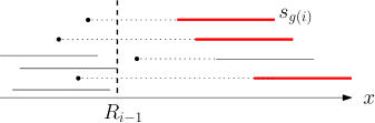
Figure 2: Illustrating the set $S_{i2}$. The segments are the covering intervals of sensors. The red thick segments correspond to the sensors in $S_{i2}$. The four black points corresponding to the values $x_{k}^{l}-r$ of the four sensors $x_{k}$ to the right of $R_{i-1}$. The sensor $s_{g(i)}$ is labeled.

4.2 The Algorithm Correctness

The correctness proof is similar to that for the algorithm in [15], so we briefly discuss it.

If the decision algorithm reports $\lambda\geq\lambda^{*}$, say, in the $i$-th step, then according to our algorithm, the configuration $C_{i}$ is a feasible solution. Below, we show that if the algorithm reports $\lambda<\lambda^{*}$, then $\lambda$ is indeed not a feasible value.

We first note that due to our jump-over procedure and our general position assumption, $R_{i}$ cannot be at the right endpoint of a barrier, and thus $p^{+}(R_{i})$ must be a point of a barrier.

An interval on $L$ is said to be left-aligned if its left side is closed and equal to $0$ and its right side is open. The algorithm correctness will be easily shown with the following Lemma 9. The proof of the lemma is very similar to Lemma 1 in [15], so we omit it.

Lemma 9

Consider any configuration $C_{i}$. Suppose $S^{\prime}_{i}$ is the set of sensors in $S$ whose right extensions are at most $R_{i}$ in $C_{i}$. Then, the interval $[0,R_{i})$ is the largest possible left-aligned interval such that all barrier points in the interval can be covered by the sensors of $S^{\prime}_{i}$ with respect to $\lambda$ (i.e., the moving distance of each sensor of $S^{\prime}_{i}$ is at most $\lambda$).

Suppose our algorithm reports $\lambda<\lambda^{*}$ in the $i$-th step. We show that $\lambda$ is not a feasible value. Indeed, according to our algorithm, $R_{i-1}<\beta$ and $S_{i1}=S_{i2}=\emptyset$ in the configuration $C_{i-1}$. Let $S_{i-1}^{\prime}$ be the set of sensors whose right extensions are at most $R_{i-1}$ in $C_{i-1}$. On the one hand, by Lemma 9 (replacing index $i$ in the lemma by $i-1$), $[0,R_{i-1})$ is the largest left-aligned interval such that all barrier points in the interval that can be covered by the sensors in $S^{\prime}_{i-1}$. On the other hand, since both $S_{i1}$ and $S_{i2}$ are empty, no sensor in $S\setminus S^{\prime}_{i-1}$ can cover the point $p^{+}(R_{i-1})$. Recall that $p^{+}(R_{i-1})$ is a barrier point not covered by any sensor in $S_{i-1}$. Due to $R_{i-1}<\beta$, we conclude that sensors of $S$ cannot cover all barrier points in the interval $[0,p^{+}(R_{i-1})]\subseteq[0,\beta]$ with respect to $\lambda$. Thus, $\lambda$ is not a feasible value. This establishes the correctness of our decision algorithm.

4.3 The Algorithm Implementation

The implementation is similar to that in [15] and we briefly discuss it. We first implement the algorithm in $O(m+n\log n)$ time, and then we reduce the time to $O(m+n\log\log n)$ under certain assumption. Then latter result will be useful in Section 5.

We first move each sensor $s_{i}$ to $x_{i}^{r}$ and thus obtain the configuration $C_{0}$. Then, we sort the extensions of all sensors in $C_{0}$, and merge the sorted list with the sorted sequence of the endpoints of all barriers. To maintain the set $S_{i1}$ during the algorithm, we sweep a point $p$ on $L$ from left to right. During the sweeping, when $p$ encounters the left (resp., right) extension of a sensor, we insert the sensor into $S_{i1}$ (resp., delete it from $S_{i1}$). In this way, in each $i$-th step of the algorithm, when $p$ is at $R_{i-1}$, $S_{i1}$ is available.

If $S_{i1}\neq\emptyset$, we pick an arbitrary sensor in $S_{i1}$ as $s_{g(i)}$. To store the set $S_{i1}$, since sensors have the same range, the earlier a sensor is inserted into $S_{i1}$, the earlier it is deleted from $S_{i1}$. Thus, we can simply use a first-in-first-out queue to store $S_{i1}$ such that each insertion/deletion can be done in constant time. We can always take the front sensor in the queue as $s_{g(i)}$.

If $S_{i1}=\emptyset$, then we need to compute $S_{i2}$. To maintain $S_{i2}$ during the sweeping of $p$, we do the following. Initially when we do the sorting as discussed above, we also sort the $n$ values $x_{i}^{l}-r$ for all $1\leq i\leq n$. During the sweeping of $p$, if $p$ encounters a point $x_{k}^{l}-r$ for some sensor $s_{k}$, we insert $s_{k}$ to $S_{i2}$, and if $p$ encounters a left extension of some sensor $s_{k}$, we delete $s_{k}$ from $S_{i2}$. In this way, when $p$ is at $R_{i-1}$, $S_{i2}$ is available. If $S_{i2}\neq\emptyset$, we need to find the leftmost sensor in $S_{i2}$ as $s_{g(i)}$, for which we use a balanced binary search tree $T$ to store all sensors of $S_{i2}$ where the “key” of each sensor $s_{k}$ is the value $x_{k}^{r}$. $T$ can support each of the following operations on $S_{i2}$ in $O(\log n)$ time: inserting a sensor, deleting a sensor, finding the leftmost sensor.

If $s_{g(i)}$ is from $S_{i1}$, then we do not need to move $s_{g(i)}$. We proceed to sweep $p$ as usual. If $s_{g(i)}$ is from $S_{i2}$, we need to move $s_{g(i)}$ leftwards to $x^{\prime}_{g(i)}=R_{i-1}+r$. Since $s_{g(i)}$ is moved, we should also update the original sorted list including the extensions of all sensors in $C_{0}$ to guide the future sweeping of $p$. To avoid the explicit update, we use a flag table for all sensor extensions in $C_{0}$. Initially, every table entry is valid. If $s_{g(i)}$ is moved, then we set the table entries of the two extensions of the sensor invalid. During the sweeping of $p$, when $p$ encounters a sensor extension, we first check the table to see whether the extension is still valid. If yes, then we proceed as usual; otherwise we ignore the event. This only costs extra constant time for each event. In addition, we calculate $R_{i}$ as discussed before, and the jump-over procedure can be implemented in $O(1)$ time since the barrier endpoints are also sorted.

To analyze the running time, since the barriers are given sorted on $L$, the sorting step takes $O(m+n\log n)$. Since there are $O(n)$ operations on the tree $T$, the total time of the algorithm is $O(m+n\log n)$. Thus we obtain the following result.

Theorem 4.1

Given any value $\lambda$, we can determine whether $\lambda\geq\lambda^{*}$ in $O(m+n\log n)$ time.

Our algorithm in Section 5 will perform feasibility tests multiple times, for which we have the following result.

Lemma 10

Suppose the values $x_{i}^{r}$ for all $i=1,2,\ldots,n$ are already sorted. We can determine whether $\lambda\geq\lambda^{*}$ in $O(m+n\log\log n)$ time for any $\lambda$.

Proof

Our $O(m+n\log n)$ time implementation is dominated by two parts. The first part is the sorting. The second part is on performing the operations on the set $S_{i2}$, each taking $O(\log n)$ time by using the tree $T$. The rest of the algorithm together takes $O(n+m)$ time. Because the values $x_{i}^{r}$ for all $i=1,2,\ldots,n$ are already sorted and the barriers are also given sorted, the sorting step takes $O(n+m)$ time.

Recall that the keys of the sensors of $T$ are the values $x_{k}^{r}$. Let $Q=\{x_{k}^{r}\ |\ 1\leq k\leq n\}$. For each sensor $s_{k}$, we use $rank(s_{k})$ to denote the rank of $x_{k}^{r}$ in $Q$ (i.e., $rank(s_{k})=t$ if $x_{k}^{r}$ is the $t$-th smallest value in $Q$). Since $Q$ is already sorted, all sensor ranks can be computed in $O(n)$ time. It is easy to see that the leftmost sensor of $T$ is the sensor with the smallest rank. Therefore, we can also use the ranks as the keys of sensors of $T$, and the advantage of doing so is that the rank of each sensor is an integer in $[1,n]$. Hence, instead of using a balanced binary search tree, we can use an integer data structure, e.g., the van Emde Boas Tree (or vEB tree for short) [6], to maintain $S_{i2}$. The vEB tree can support each of the following operations on $S_{i2}$ in $O(\log\log n)$ time [6]: inserting a sensor, deleting a sensor, and finding the sensor with the smallest rank. Using a vEB tree, all operations on $S_{i2}$ in the algorithm can be performed in $O(n\log\log n)$ time. The lemma thus follows. ∎

5 Solving the Problem MBC

In this section, we solve the problem MBC. It suffices to compute $\lambda^{*}$.

It might be tempting to use the similar algorithm scheme as that for the line-constrained version of the problem in Section 3, i.e., first identify a set of candidate values for $\lambda^{*}$ and then search the set to find $\lambda^{*}$ by using the decision algorithm. However, we find some obstacles to do so. For example, as mentioned in Section 1.2, one major difficulty of the problem is that we do not know the order of the sensors of $S$ on $L$ in an optimal solution. Because of that, it is not clear how to identify a relatively small set (e.g., of polynomial size) of candidate values for $\lambda^{*}$. Therefore, we have to resort to other techniques to tackle the problem. The high-level scheme of our algorithm is similar to that in [15], although some low-level details are different.

In this section, we use $x_{i}^{r}(\lambda)$ to refer to $x_{i}^{r}$ for any $\lambda$, so that we consider $x_{i}^{r}(\lambda)$ as a function on $\lambda\in[0,\infty]$, which actually defines a half of the upper branch (on the right side of the $y$-axis) of a hyperbola (in contrast, the corresponding function in [15] is linear, and thus our result is more general than that in [15]). Let $\sigma$ be the order of the values $x_{i}^{r}(\lambda^{*})$ for all $i\in[1,n]$. To make use of Lemma 10, we first run a preprocessing step in Lemma 11. Note that Lemma 11 is not from [15], and we will discuss in Section 6 that the technique can be used to reduce the space complexity of the algorithm in [15].

Lemma 11

With $O(n\log^{3}n+m\log^{2}n)$ time preprocessing, we can compute $\sigma$ and an interval $(\lambda^{*}_{1},\lambda^{*}_{2}]$ containing $\lambda^{*}$ such that $\sigma$ is also the order of the values $x_{i}^{r}(\lambda)$ for any $\lambda\in(\lambda^{*}_{1},\lambda^{*}_{2}]$.

Proof

To compute $\sigma$, we apply Megiddo’s parametric search [17] to sort the values $x_{i}^{r}(\lambda^{*})$ for $i\in[1,n]$, using the decision algorithm in Theorem 4.1. Indeed, recall that $x_{i}^{r}(\lambda)=x_{i}+\sqrt{\lambda^{2}-y_{i}^{2}}$. Hence, as $\lambda$ increases, $x_{i}^{r}(\lambda)$ is a (strictly) increasing function. For any two indices $i$ and $j$, there is at most one root on $\lambda\in[0,\infty)$ for the equation: $x_{i}^{r}(\lambda)=x_{j}^{r}(\lambda)$. Therefore, we can apply Megiddo’s parametric search [17] to do the sorting. The total time is $O((\tau+n)\log^{2}n)$, where $\tau$ is the running time of the decision algorithm. By Theorem 4.1, $\tau=O(m+n\log n)$. Hence, the total time for computing $\sigma$ is $O(m\log^{2}n+n\log^{3}n)$.

In addition, Megiddo’s parametric search [17] will return an interval $(\lambda^{*}_{1},\lambda^{*}_{2}]$ such that it contains $\lambda^{*}$ and $\sigma$ is also the order of the values $x_{i}^{r}(\lambda)$ for any $\lambda\in(\lambda^{*}_{1},\lambda^{*}_{2}]$. ∎

Note that $\lambda^{*}$ is the smallest feasible value. As $\lambda^{*}\in(\lambda^{*}_{1},\lambda^{*}_{2}]$, our subsequent feasible tests will be only on values $\lambda\in(\lambda^{*}_{1},\lambda^{*}_{2})$ because if $\lambda\leq\lambda^{*}_{1}$, then $\lambda$ is not feasible and if $\lambda\geq\lambda^{*}_{2}$, then $\lambda$ is feasible. Lemmas 10 and 11 together lead to the following result.

Lemma 12

Each feasibility test can be done in $O(m+n\log\log n)$ time for any $\lambda\in(\lambda^{*}_{1},\lambda^{*}_{2})$.

To compute $\lambda^{*}$, we “parameterize” our decision algorithm with $\lambda$ as a parameter. Although we do not know $\lambda^{*}$, we execute the decision algorithm in such a way that it computes the same subset of sensors $s_{g(1)},s_{g(2)},\ldots$ as would be obtained if we ran the decision algorithm on $\lambda=\lambda^{*}$.

Recall that for any $\lambda$, step $i$ of our decision algorithm computes the sensor $s_{g(i)}$, the set $S_{i}=\{s_{g(1)},s_{g(2)},\ldots,s_{g(i)}\}$, and the value $R_{i}$, and obtains the configuration $C_{i}$. In the following, we often consider $\lambda$ as a variable rather than a fixed value. Thus, we will use $S_{i}(\lambda)$ (resp., $R_{i}(\lambda)$, $s_{g(i)}(\lambda)$, $C_{i}(\lambda)$, $x_{i}^{r}(\lambda)$) to refer to the corresponding $S_{i}$ (resp., $R_{i}$, $s_{g(i)}$, $C_{i}$, $x_{i}^{r}$). Our algorithm has at most $n$ steps. Consider a general $i$-th step for $i\geq 1$. Right before the step, we have an interval $(\lambda^{1}_{i-1},\lambda_{i-1}^{2}]$ and a sensor set $S_{i-1}(\lambda)$, such that the following algorithm invariants hold.

1. $\lambda^{*}\in(\lambda^{1}_{i-1},\lambda_{i-1}^{2}]$.

2. The set $S_{i-1}(\lambda)$ is the same (with the same order) for all values $\lambda\in(\lambda^{1}_{i-1},\lambda_{i-1}^{2})$.

3. $R_{i-1}(\lambda)$ on $\lambda\in(\lambda^{1}_{i-1},\lambda_{i-1}^{2})$ is either constant or equal to $x_{j}+\sqrt{\lambda^{2}-y_{j}^{2}}+c$ for some constant $c$ and some sensor $s_{j}$, and the function $R_{i-1}(\lambda)$ is explicitly maintained by the algorithm.

4. $R_{i-1}(\lambda)<\beta$ for all $\lambda\in(\lambda^{1}_{i-1},\lambda_{i-1}^{2})$.

Initially when $i=1$, we let $\lambda_{0}^{1}=\lambda^{*}_{1}$ and $\lambda_{0}^{2}=\lambda^{*}_{2}$. Since $S_{0}(\lambda)=\emptyset$ and $R_{0}(\lambda)=0$ for any $\lambda$, by Lemma 11, all invariants hold for $i=1$. In general, the $i$-th step will either compute $\lambda^{*}$, or obtain an interval $(\lambda^{1}_{i},\lambda_{i}^{2}]\subseteq(\lambda^{1}_{i-1},\lambda_{i-1}^{2}]$ and a sensor $s_{g(i)}(\lambda)$ with $S_{i}(\lambda)=S_{i-1}(\lambda)\cup\{s_{g(i)}(\lambda)\}$. The running time of the step is $O((m+n\log\log n)(\log n+\log m))$. The details are given below.

5.1 The Algorithm

We assume $\lambda^{*}\neq\lambda_{i-1}^{2}$ and thus $\lambda^{*}$ is in $(\lambda_{i-1}^{1},\lambda_{i-1}^{2})$. Our following algorithm can proceed without this assumption and we make the assumption only for explaining the rationale of our approach. Since $\lambda^{*}\in(\lambda_{i-1}^{1},\lambda_{i-1}^{2})$, according to our algorithm invariants, for all $\lambda\in(\lambda_{i-1}^{1},\lambda_{i-1}^{2})$, $S_{i-1}(\lambda)$ is the same as $S_{i-1}(\lambda^{*})$. We simulate the decision algorithm on $\lambda=\lambda^{*}$. To determine the sensor $s_{g(i)}(\lambda^{*})$, we first compute the set $S_{i1}(\lambda^{*})$, as follows.

Consider any sensor $s_{k}$ in $S\setminus S_{i-1}(\lambda)$. Its position in $C_{i-1}(\lambda)$ is $x_{k}^{r}(\lambda)=x_{k}+\sqrt{\lambda^{2}-y_{k}^{2}}$, which is an increasing function of $\lambda$. Thus, both the left and the right extensions of $s_{k}$ in $C_{i-1}(\lambda)$ are increasing functions of $\lambda$. Suppose $f(\lambda)$ is either the left or the right extension of $s_{k}$ in $C_{i-1}(\lambda)$. According to our algorithm invariants, $R_{i-1}(\lambda)$ on $\lambda\in(\lambda^{1}_{i-1},\lambda_{i-1}^{2})$ is either constant or equal to $x_{j}+\sqrt{\lambda^{2}-y_{j}^{2}}+c$ for some constant $c$ and some sensor $s_{j}$. We claim that there is at most one value $\lambda$ in $(\lambda^{1}_{i-1},\lambda_{i-1}^{2})$ such that $R_{i-1}(\lambda)=f(\lambda)$. Indeed, if $R_{i-1}(\lambda)$ is constant, then this is obviously true; otherwise, this is also true because each of $f(\lambda)$ and $R_{i-1}(\lambda)$ on $\lambda\in[0,\infty)$ defines a half branch of a hyperbola (and thus they have at most one intersection in $(\lambda^{1}_{i-1},\lambda_{i-1}^{2})$).

Let $S^{\prime}=S\setminus S_{i-1}(\lambda)$. If we increase $\lambda$ from $\lambda^{1}_{i-1}$ to $\lambda^{2}_{i-1}$, an “event” happens if $R_{i-1}(\lambda)$ is equal to the left or right extension value of a sensor $s_{k}\in S^{\prime}$ at some value of $\lambda$ (called an event value). Note that $S_{i1}(\lambda)$ does not change between any two adjacent events. To compute $S_{i1}(\lambda^{*})$, we first compute all event values, and this can be done in $O(n)$ time by using the function $R_{i-1}(\lambda)$ and all left and right extension functions of the sensors in $S^{\prime}$. Let $\Lambda$ denote the set of all event values, and we also add $\lambda^{1}_{i-1}$ and $\lambda^{2}_{i-1}$ to $\Lambda$. We then sort all values in $\Lambda$. Using the feasibility test in Lemma 12, we do binary search to find two adjacent values $\lambda_{1}$ and $\lambda_{2}$ in the sorted list of $\Lambda$ such that $\lambda^{*}\in(\lambda_{1},\lambda_{2}]$. Note that $(\lambda_{1},\lambda_{2}]\subseteq(\lambda^{1}_{i-1},\lambda_{i-1}^{2}]$. Since $|\Lambda|=O(n)$, the binary search uses $O(\log n)$ feasibility tests, which takes overall $O(m\log n+n\log n\log\log n)$ time.

We make another assumption that $\lambda^{*}\neq\lambda_{2}$. Again, this assumption is only for the explanation and the following algorithm can proceed without this assumption. Under the assumption, for any $\lambda\in(\lambda_{1},\lambda_{2})$, the set $S_{i1}(\lambda)$ is exactly $S_{i1}(\lambda^{*})$. Hence, we can compute $S_{i1}(\lambda^{*})$ by taking any $\lambda\in(\lambda_{1},\lambda_{2})$ and explicitly computing $S_{i1}(\lambda)$ in $O(n)$ time.

The above has computed $S_{i1}(\lambda^{*})$. If $S_{i1}(\lambda^{*})\neq\emptyset$, we take an arbitrary sensor of $S_{i1}(\lambda^{*})$ as $s_{g(i)}(\lambda^{*})$. Further, we let $\lambda_{i}^{1}=\lambda_{1}$, $\lambda_{i}^{2}=\lambda_{2}$, and $S_{i}(\lambda)=S_{i-1}(\lambda)\cup\{s_{g(i)}(\lambda^{*})\}$.

If $S_{i1}(\lambda^{*})=\emptyset$, then we need to compute the set $S_{i2}(\lambda^{*})$. Since $\lambda^{*}\in(\lambda_{1},\lambda_{2})\subseteq(\lambda^{1}_{i-1},\lambda_{i-1}^{2})$, according to our algorithm invariants, $R_{i-1}(\lambda)$ is a nondecreasing function on $\lambda\in(\lambda_{1},\lambda_{2})$. For each sensor $s_{k}\in S$, $x_{k}-\sqrt{\lambda^{2}-y_{k}^{2}}-r$ is a decreasing function on $\lambda\in(\lambda_{1},\lambda_{2})$. Therefore, the interval $(\lambda_{1},\lambda_{2})$ contains at most one value $\lambda$ such that $R_{i-1}(\lambda)=x_{k}-\sqrt{\lambda^{2}-y_{k}^{2}}-r$. If we increase $\lambda$ from $\lambda_{1}$ to $\lambda_{2}$, an “event” happens when $R_{i-1}(\lambda)$ is equal to $x_{k}-\sqrt{\lambda^{2}-y_{k}^{2}}-r$ for some sensor $s_{k}\in S^{\prime}$ at some event value $\lambda$. Also, the set $S_{i2}(\lambda)$ is fixed between any two adjacent events. Hence, we use the following way to compute $S_{i2}(\lambda^{*})$.

We first compute the set $\Lambda$ of all event values, and also add $\lambda_{1}$ and $\lambda_{2}$ to $\Lambda$. After sorting all values of $\Lambda$, by using our decision algorithm, we do binary search to find two adjacent values $\lambda_{1}^{\prime}$ and $\lambda_{2}^{\prime}$ in the sorted list of $\Lambda$ with $\lambda^{*}\in(\lambda_{1}^{\prime},\lambda_{2}^{\prime}]$. Note that $(\lambda_{1}^{\prime},\lambda_{2}^{\prime}]\subseteq(\lambda_{1},\lambda_{2}]$. Since $|\Lambda|=O(n)$, the binary search calls the decision algorithm $O(\log n)$ times, which takes $O(m\log n+n\log n\log\log n)$ time in total. Since $S_{i2}(\lambda)$ is the same for all $\lambda\in(\lambda_{1}^{\prime},\lambda_{2}^{\prime})$, we take an arbitrary value $\lambda\in(\lambda^{\prime}_{1},\lambda^{\prime}_{2})$ and compute $S_{i2}(\lambda)$ explicitly in $O(n)$ time.

Lemma 13

If $S_{i2}(\lambda)=\emptyset$, then $\lambda^{*}$ is in $\{\lambda_{i-1}^{2},\lambda_{2},\lambda_{2}^{\prime}\}$.

Proof

Assume to the contrary that $\lambda^{*}\not\in\{\lambda_{i-1}^{2},\lambda_{2},\lambda_{2}^{\prime}\}$. Then, our previous two assumptions on $\lambda^{*}$ are true and $\lambda^{*}\in(\lambda_{1}^{\prime},\lambda_{2}^{\prime})$. According to our algorithm, $S_{i2}(\lambda^{*})=S_{i2}(\lambda)=\emptyset$ (and $S_{i1}(\lambda^{*})=S_{i1}(\lambda)=\emptyset$). This means that if we applied the decision algorithm on $\lambda=\lambda^{*}$, the sensor $s_{g(i)}(\lambda^{*})$ would not exist. In other words, the decision algorithm would stop after the first $i-1$ steps, i.e., the decision algorithm would only use sensors in $S_{i-1}(\lambda^{*})$ to cover all barriers.

On the other hand, according to our algorithm invariants, $R_{i-1}(\lambda)<\beta$ for all $\lambda\in(\lambda_{i-1}^{1},\lambda_{i-1}^{2})$. Since $\lambda^{*}\in(\lambda_{1}^{\prime},\lambda_{2}^{\prime})\subseteq(\lambda_{i-1}^{1},\lambda_{i-1}^{2})$, $R_{i-1}(\lambda^{*})<\beta$, but this contradicts with that all barriers are covered by the sensors of $S_{i-1}(\lambda^{*})$ after the first $i-1$ steps of the decision algorithm. ∎

By Lemma 13, if $S_{i2}(\lambda)=\emptyset$, then $\lambda^{*}$ is the smallest feasible value of $\{\lambda_{i-1}^{2},\lambda_{2},\lambda_{2}^{\prime}\}$, which can be found by performing three feasibility tests. Otherwise, we proceed as follows.

We make the third assumption that $\lambda^{*}\neq\lambda_{2}^{\prime}$. Thus, $\lambda^{*}\in(\lambda_{1}^{\prime},\lambda_{2}^{\prime})$ and $S_{i2}(\lambda^{*})=S_{i2}(\lambda)$ for any $\lambda\in(\lambda_{1}^{\prime},\lambda_{2}^{\prime})$. Next, we compute $s_{g(i)}(\lambda^{*})$, i.e., the leftmost sensor of $S_{i2}(\lambda^{*})$. Although $S_{i2}(\lambda)$ is the same for all $\lambda\in(\lambda_{1}^{\prime},\lambda_{2}^{\prime})$, the leftmost sensor of $S_{i2}(\lambda)$ may not be the same for all $\lambda\in(\lambda_{1}^{\prime},\lambda_{2}^{\prime})$. For each sensor $s_{k}\in S_{i2}(\lambda)$ and any $\lambda\in(\lambda_{1}^{\prime},\lambda_{2}^{\prime})$, the location of $s_{k}$ in the configuration $C_{i-1}(\lambda)$ is $x_{k}^{r}(\lambda)$. As discussed before, $x_{k}^{r}(\lambda)$ for $\lambda\in(\lambda_{1}^{\prime},\lambda_{2}^{\prime})$ defines a piece of the upper branch of a hyperbola in the 2D coordinate system in which the $x$-coordinates correspond to the $\lambda$ values and the $y$-coordinates correspond to $x_{k}^{r}(\lambda)$ values. We consider the lower envelope $\mathcal{L}$ of the functions $x_{k}^{r}(\lambda)$ defined by all sensors $s_{k}$ of $S_{i2}(\lambda)$. For each point $q$ of $\mathcal{L}$, suppose $q$ lies on the function defined by a sensor $s_{k}$ and $q$’s $x$-coordinate is $\lambda_{q}$. If $\lambda=\lambda_{q}$, then the leftmost sensor of $S_{i2}(\lambda)$ is $s_{k}$. This means that each curve segment of $\mathcal{L}$ defined by one sensor corresponds to the same leftmost sensor of $S_{i2}(\lambda)$. Based on this observation, we compute $s_{g(i)}(\lambda^{*})$ as follows.

Since the functions $x_{k}^{r}(\lambda)$ and $x_{j}^{r}(\lambda)$ of two sensors $s_{k}$ and $s_{j}$ have at most one intersection in $(\lambda_{1}^{\prime},\lambda_{2}^{\prime})$, the number of vertices of the lower envelope $\mathcal{L}$ is $O(n)$ and $\mathcal{L}$ can be computed in $O(n\log n)$ time [2, 13, 20]. Let $\Lambda$ be the set of the $x$-coordinates of the vertices of $\mathcal{L}$. We also add $\lambda_{1}^{\prime}$ and $\lambda_{2}^{\prime}$ to $\Lambda$. After sorting all values of $\Lambda$, by using our decision algorithm, we do binary search on the sorted list of $\Lambda$ to find two adjacent values $\lambda_{1}^{\prime\prime}$ and $\lambda_{2}^{\prime\prime}$ such that $\lambda^{*}\in(\lambda_{1}^{\prime\prime},\lambda_{2}^{\prime\prime}]$. Note that $(\lambda_{1}^{\prime\prime},\lambda_{2}^{\prime\prime}]\subseteq(\lambda_{1}^{\prime},\lambda_{2}^{\prime}]$. Since $\lambda_{1}^{\prime\prime}$ and $\lambda_{2}^{\prime\prime}$ are two adjacent values of the sorted $\Lambda$, by our above analysis, there is a sensor that is always the leftmost sensor of $S_{i2}(\lambda)$ for all $\lambda\in(\lambda_{1}^{\prime\prime},\lambda_{2}^{\prime\prime}]$. To find the sensor, we can take any value $\lambda$ in $(\lambda_{1}^{\prime\prime},\lambda_{2}^{\prime\prime})$ and explicitly compute the locations of sensors in $S_{i2}(\lambda)$. The above computes $s_{g(i)}(\lambda^{*})$ in $O(m\log n+n\log n\log\log n)$ time.

Finally, we let $\lambda_{i}^{1}=\lambda_{1}^{\prime\prime}$, $\lambda_{i}^{2}=\lambda_{2}^{\prime\prime}$, and $S_{i}(\lambda)=S_{i-1}(\lambda)\cup\{s_{g(i)}(\lambda^{*})\}$.

If the above computes $\lambda^{*}$, then we terminate the algorithm. Otherwise, we obtain an interval $(\lambda_{i}^{1},\lambda_{i}^{2}]\subseteq(\lambda_{i-1}^{1},\lambda_{i-1}^{2}]$ that contains $\lambda^{*}$ and the set $S_{i}(\lambda)$. If $s_{g(i)}(\lambda)\in S_{i1}(\lambda)$, then $R_{i}(\lambda)$ is equal to $x_{g(i)}+\sqrt{\lambda^{2}-y_{g(i)}^{2}}+r$. If $s_{g(i)}(\lambda)\in S_{i2}(\lambda)$, then $R_{i}(\lambda)=R_{i-1}(\lambda)+2r$. According to the third algorithm invariant, $R_{i-1}(\lambda)$ is either constant or equal to $x_{j}+\sqrt{\lambda^{2}-y_{j}^{2}}+c$ for some constant $c$ and some sensor $s_{j}$. Therefore, regardless of $s_{g(i)}(\lambda)\in S_{i1}(\lambda)$ or $s_{g(i)}(\lambda)\in S_{i2}(\lambda)$, $R_{i}(\lambda)$ is either constant or equal to $x_{j^{\prime}}+\sqrt{\lambda^{2}-y_{j^{\prime}}^{2}}+c^{\prime}$ for some constant $c^{\prime}$ and some sensor $s_{j^{\prime}}$, which establishes the third algorithm invariant for $R_{i}(\lambda)$.

If it is not true that $R_{i}(\lambda)<\beta$ for all $\lambda\in(\lambda_{i}^{1},\lambda_{i}^{2})$, then we preform some additional processing as follows. We first have the following lemma.

Lemma 14

If it is not true that $R_{i}(\lambda)<\beta$ for all $\lambda\in(\lambda_{i}^{1},\lambda_{i}^{2})$, then $R_{i}(\lambda)$ is strictly increasing on $(\lambda_{i}^{1},\lambda_{i}^{2})$ and there is a single value $\lambda^{\prime}\in(\lambda_{i}^{1},\lambda_{i}^{2})$ such that $R_{i}(\lambda^{\prime})=\beta$.

Proof

The proof is almost the same as that of Lemma 4 in [15] and we include it here for the sake of completeness.

Since it is not true that $R_{i}(\lambda)<\beta$ for all $\lambda\in(\lambda_{i}^{1},\lambda_{i}^{2})$, either $R_{i}(\lambda)>\beta$ for all $\lambda\in(\lambda_{i}^{1},\lambda_{i}^{2})$, or there is a value $\lambda^{\prime}\in(\lambda_{i}^{1},\lambda_{i}^{2})$ with $R_{i}(\lambda^{\prime})=\beta$. We first argue that the former case cannot happen.

Assume to the contrary that $R_{i}(\lambda)>\beta$ for all $\lambda\in(\lambda_{i}^{1},\lambda_{i}^{2})$. Then, $R_{i}(\lambda^{\prime})>\beta$ for any $\lambda^{\prime}\in(\lambda_{i}^{1},\lambda^{*})$ since $\lambda^{*}\in(\lambda_{i}^{1},\lambda_{i}^{2}]$. But this would imply that we have found a feasible solution using only sensors in $S_{i}(\lambda)$ and the maximum movement of all sensors in $S_{i}(\lambda)$ is at most $\lambda^{\prime}<\lambda^{*}$, contradicting with that $\lambda^{*}$ is the maximum moving distance in an optimal solution.

Hence, there is a value $\lambda^{\prime}\in(\lambda_{i}^{1},\lambda_{i}^{2})$ with $R_{i}(\lambda^{\prime})=\beta$. Next, we show that $R_{i}(\lambda)$ must be a strictly increasing function. Assume to the contrary this is not true. Then, $R_{i}(\lambda)$ must be constant on $(\lambda_{i}^{1},\lambda_{i}^{2})$. Thus, $R_{i}(\lambda)=\beta$ for all $\lambda\in(\lambda_{i}^{1},\lambda_{i}^{2})$. Since $\lambda^{*}\in(\lambda_{i}^{1},\lambda_{i}^{2}]$, let $\lambda^{\prime}$ be any value in $(\lambda_{i}^{1},\lambda^{*})$. Hence, $R_{i}(\lambda^{\prime})=\beta$, and as above, $\lambda^{\prime}$ is a feasible value. However, $\lambda^{\prime}<\lambda^{*}$ incurs contradiction. ∎

By Lemma 14, we compute the value $\lambda^{\prime}\in(\lambda_{i}^{1},\lambda_{i}^{2})$ such that $R_{i}(\lambda^{\prime})=\beta$. This means that all barriers are covered by the sensors of $S_{i}(\lambda^{\prime})$ in $C_{i}(\lambda^{\prime})$, and thus $\lambda^{\prime}$ is a feasible value and $\lambda^{*}\in(\lambda_{i}^{1},\lambda^{\prime}]$. Because $R_{i}(\lambda)$ is strictly increasing, $R_{i}(\lambda)<\beta$ for all $\lambda\in(\lambda_{i}^{1},\lambda^{\prime})$. We update $\lambda_{i}^{2}$ to $\lambda^{\prime}$.

In either case, $R_{i}(\lambda)<\beta$ now holds for all $\lambda\in(\lambda_{i}^{1},\lambda_{i}^{2})$. Finally, we perform the jump-over procedure, as follows (this step is not needed in [15]).

If $R_{i}(\lambda)$ is a constant and $R_{i}(\lambda)$ is not in the interior of a barrier, then we set $R_{i}(\lambda)$ to the left endpoint of the next barrier. If $R_{i}(\lambda)$ is an increasing function, then we do the following. If we increase $\lambda$ from $\lambda_{i}^{1}$ to $\lambda_{i}^{2}$, an event happens if $R_{i}(\lambda)$ is equal to the left or right endpoint of a barrier at some event value of $\lambda$. During the increasing of $\lambda$, between any two adjacent events, $R_{i}(\lambda)$ is either always in the interior of a barrier or is always between two barriers. We compute all event values in $O(m)$ time by using the function $R_{i}(\lambda)$ and the endpoints of all barriers. Let $\Lambda$ denote the set of all event values, and we also add $\lambda^{1}_{i}$ and $\lambda^{2}_{i}$ to $\Lambda$. After sorting all values in $\Lambda$, using the decision algorithm in Lemma 12, we do binary search on the sorted list of $\Lambda$ to find two adjacent values $\lambda_{1}$ and $\lambda_{2}$ such that $\lambda^{*}\in(\lambda_{1},\lambda_{2}]$. Note that $(\lambda_{1},\lambda_{2}]\subseteq(\lambda^{1}_{i},\lambda_{i}^{2}]$. Since $|\Lambda|=O(m)$, the binary search calls the decision algorithm $O(\log m)$ times, which takes overall $O(m\log m+n\log\log n\log m)$ time. Finally, we reset $\lambda_{i}^{1}=\lambda_{1}$ and $\lambda_{i}^{2}=\lambda_{2}$.

This completes the $i$-th step of the algorithm, which runs in $O((m+n\log\log n)\cdot(\log m+\log n))$ time. If $\lambda^{*}$ is not computed in this step, then it can be verified that all algorithm variants are maintained (the analysis is similar to that in [15], so we omit it). The algorithm will compute $\lambda^{*}$ after at most $n$ steps as there are $n$ sensors. The total time of the algorithm is $O(n\cdot(m+n\log\log n)\cdot(\log m+\log n))$, which is bounded by $O(nm\log m+n^{2}\log n\log\log n)$ as shown in the following theorem. Note that the space of the algorithm is $O(n)$.

Theorem 5.1

The problem MBC can be solved in $O(nm\log m+n^{2}\log n\log\log n)$ time and $O(n)$ space.

Proof

As discussed before, the running time of the algorithm is $O(n\cdot(m+n\log\log n)\cdot(\log m+\log n))$, which is $O(nm\log m+n^{2}\log n\log\log n+nm\log n+n^{2}\log m\log\log n)$. We claim that $nm\log n+n^{2}\log m\log\log n=O(nm\log m+n^{2}\log n\log\log n)$. Indeed, if $m\leq n\log\log n$, then $nm\log n=O(n^{2}\log n\log\log n)$ and $n^{2}\log m\log\log n=O(n^{2}\log n\log\log n)$; otherwise, $nm\log n=O(nm\log m)$ and $n^{2}\log m\log\log n=O(nm\log m)$. ∎

6 Concluding Remarks

As mentioned before, the high-level scheme of our algorithm for MBC is similar to those in [15]. However, a new technique we propose in this paper can help reduce the space complexity of the algorithm in [15]. Specifically, Lee et al. [15] solved the line-constrained problem in $O(n^{2}\log n\log\log n)$ time and $O(n^{2})$ space for the case where $m=1$, sensors have the same range, and sensors have weights. If we apply the similar preprocessing as in Lemma 11, then the space complexity of the algorithm [15] can be reduced to $O(n)$ while the time complexity does not change asymptotically.

References

- [1] A.M. Andrews and H. Wang. Minimizing the aggregate movements for interval coverage. Algorithmica, 78:47–85, 2017.
- [2] M.J. Atallah. Some dynamic computational geometry problems. Computers and Mathematics with Applications, 11:1171–1181, 1985.
- [3] B. Bhattacharya, B. Burmester, Y. Hu, E. Kranakis, Q. Shi, and A. Wiese. Optimal movement of mobile sensors for barrier coverage of a planar region. Theoretical Computer Science, 410(52):5515–5528, 2009.
- [4] D.Z. Chen, Y. Gu, J. Li, and H. Wang. Algorithms on minimizing the maximum sensor movement for barrier coverage of a linear domain. Discrete and Computational Geometry, 50:374–408, 2013.
- [5] D.Z. Chen, X. Tan, H. Wang, and G. Wu. Optimal point movement for covering circular regions. Algorithmica, 72:379–399, 2015.
- [6] T. Cormen, C. Leiserson, R. Rivest, and C. Stein. Introduction to Algorithms. MIT Press, 3nd edition, 2009.
- [7] J. Czyzowicz, E. Kranakis, D. Krizanc, I. Lambadaris, L. Narayanan, J. Opatrny, L. Stacho, J. Urrutia, and M. Yazdani. On minimizing the maximum sensor movement for barrier coverage of a line segment. In Proceedings of the 8th International Conference on Ad-Hoc, Mobile and Wireless Networks, pages 194–212, 2009.
- [8] J. Czyzowicz, E. Kranakis, D. Krizanc, I. Lambadaris, L. Narayanan, J. Opatrny, L. Stacho, J. Urrutia, and M. Yazdani. On minimizing the sum of sensor movements for barrier coverage of a line segment. In Proceedings of the 9th International Conference on Ad-Hoc, Mobile and Wireless Networks, pages 29–42, 2010.
- [9] S. Dobrev, S. Durocher, M. Eftekhari, K. Georgiou, E. Kranakis, D. Krizanc, L. Narayanan, J. Opatrny, S. Shende, and J. Urrutia. Complexity of barrier coverage with relocatable sensors in the plane. Theoretical Computer Science, 579:64–73, 2015.
- [10] G.N. Frederickson. Optimal algorithms for tree partitioning. In Proceedings of the 2nd Annual ACM-SIAM Symposium of Discrete Algorithms (SODA), pages 168–177, 1991.
- [11] G.N. Frederickson. Parametric search and locating supply centers in trees. In Proceedings of the 2nd International Workshop on Algorithms and Data Structures (WADS), pages 299–319, 1991.
- [12] G.N. Frederickson and D.B. Johnson. Generalized selection and ranking: Sorted matrices. SIAM Journal on Computing, 13(1):14–30, 1984.
- [13] J. Hershberger. Finding the upper envelope of line segments in time. Information Processing Letters, 33:169–174, 1989.
- [14] S. Kumar, T.H. Lai, and A. Arora. Barrier coverage with wireless sensors. In Proceedings of the 11th Annual International Conference on Mobile Computing and Networking (MobiCom), pages 284–298, 2005.
- [15] V.C.S Lee, H. Wang, and X. Zhang. Minimizing the maximum moving cost of interval coverage. International Journal of Computational Geometry and Applications, 27:187–205, 2017.
- [16] S. Li and H. Shen. Minimizing the maximum sensor movement for barrier coverage in the plane. In Proceedings of the 2015 IEEE Conference on Computer Communications (INFOCOM), pages 244–252, 2015.
- [17] N. Megiddo. Applying parallel computation algorithms in the design of serial algorithms. Journal of the ACM, 30(4):852–865, 1983.
- [18] M. Mehrandish. On Routing, Backbone Formation and Barrier Coverage in Wireless Ad Doc and Sensor Networks. PhD thesis, Concordia University, Montreal, Quebec, Canada, 2011.
- [19] M. Mehrandish, L. Narayanan, and J. Opatrny. Minimizing the number of sensors moved on line barriers. In Proceedings of IEEE Wireless Communications and Networking Conference (WCNC), pages 653–658, 2011.
- [20] M. Sharir and P.K. Agarwal. Davenport-Schinzel Sequences and Their Geometric Applications. Cambridge University Press, New York, 1996.