The finite density scaling laws of condensation phase transition in zero range processes on scale-free networks

Abstract

The dynamics of zero-range processes on complex networks is expected to be influenced by the topological structure of underlying networks. A real space complete condensation phase transition in the stationary state may occur. We have studied the finite density effects of the condensation transition in both the stationary and dynamical zero-range process on scale-free networks. By means of grand canonical ensemble method, we predict analytically the scaling laws of the average occupation number with respect to the finite density for the steady state. We further explore the relaxation dynamics of the condensation phase transition. By applying the hierarchical evolution and scaling ansatz, a scaling law for the relaxation dynamics is predicted. Monte Carlo simulations are performed and the predicted density scaling laws are nicely validated.

I Introduction

Condensation phase transitions are abundant phenomena in nature and observed in various physical circumstances and stochastic processes. For instance, the Bose-Einstein condensation (BEC) in cold dilute atomic gases BEC , jamming in traffic flow Chow00 and granular flow Meer02 ; Meer04 , condensation of links in complex networks Krap00 ; Bian01 ; Zhang12 , to name a few. Although the equilibrium condensation phase transitions can be well described in the framework of equilibrium statistical mechanics Path11 , building a consistent theory of nonequilibrium (condensation) phase transitions remains a big challenge. How such transitions arise and what dynamical nature they may have are particularly intriguing questions to be answered. The long lasting efforts have been paid on the investigation of interacting particle systems Ligg99 . One of the important categories is so-called driven diffusive systems Schm95 . These systems are driven away from equilibrium by external forces, and may evolve toward a nonequilibrium steady state. In addition, they exhibit non-trivial behavior such like phase separation Evans98 or phase transitions (even in one spatial dimension) Evans06 .

Among above mentioned systems, the zero range processes (ZRPs), introduced by F. Spitzer Spitz70 roughly half century ago, has attracted considerable attention due to the fact that it is one of few rare examples of analytically tractable nonequilibrium models. For recent reviews, see e.g., Evans05 ; Godre07 and references therein. The prototype of ZRP is a stochastic particle system defined on one dimensional regular lattice of given number of sites and particles hop onto the nearest neighbours (NNs) with some transition rate, say, $u(n)$. This rate function depends only on the occupation number $n$ of its current position, not that of the other sites – this defines the zero-range property of the process. If $u(n)$ is decreasing in $n$, then an effective attraction between particles is presented. As a result, a condensation transition occurs if $\rho$ exceeds some critical density $\rho_{c}$, and a macroscopically finite fraction of particles condense on a single site. The condensation phase transitions in ZRPs have been studied based on periodic lattices in Evans00 ; Gross03 ; Majum05 ; Godre12 .

From the perspective of complex networks, the underlying periodic lattice of ZRPs is simply regular fully connected network. However, many natural and manmade networks are self-organized as the scale-free (SF) networks (see e.g., BA02 ; Eguil05 ; Bocca06 and references therein). The SF networks are strongly inhomogeneous and highly clustering in architecture BA99 . They also typically possess a power-law degree distribution, $\mathscr{P}_{deg}(k)\sim k^{-\gamma}$, where $k$ is the degree (i.e. number of links) of a node and the constant $\gamma$ is degree exponent. It has been demonstrated that these significant features of SF networks are important factors affected a multitude of critical phenomena Golt08 , and as well as dynamical processes Barth04 ; Sood05 ; Noh05a ; Noh05b ; Tang06 defined on them. It was found when the power exponent $\delta$ in the hopping rate $u(n)=n^{\delta}$ is smaller than a critical value $\delta_{c}$, that is, when $\delta<\delta_{c}=1/(\gamma-1)$, a finite fraction of particles are condensed into the node with the maximum degree, or the hub Noh05a . Such condensation phase transitions are driven by the interplay of the (effective) interaction between particles and the topological structure disorder of the underlying SF networks. However, to the author’ knowledge, so far the analysis of the possible effects of the finite density are still absent. In fact, one naturally expects the density plays an important role in condensation transition of ZRPs on SF networks.

In current paper we then focus on the finite density aspect of the condensation transition of the static and dynamical ZRP defined on SF networks. As we will show in the following, based on the grand canonical ensemble (GCE) approach, we predict a novel scaling law in the condensation phase transition with respect to (w.r.t.) the finite density. Another important issue we addressed in this paper is the relaxation dynamics in the condensed phase transition. A hierarchical evolution occurs in relaxation dynamics, i.e., the relaxation proceeds from small degree nodes to larger and larger degree nodes. We predict that there exist the scaling laws of the average occupation number and the inverse participation ratio (IPR) w.r.t. the finite density in both steady state and relaxation dynamics. To verify our analytical predictions, Monte Carlo simulations are fulfilled for steady state and the relaxation dynamics, respectively. These predicted finite density scaling laws are nicely confirmed.

The rest of the paper is organized as follows: in Sec. II, we present the ZRP model on SF network, and the corresponding GCE theoretical formalism. In Sec. III, we first argue the existence of the condensation phase transition, and then predicted the finite density scaling laws for such transition. Monte Carlo simulations are followed and fully confirmed previous analytical results. In Sec. IV, we explore the relaxation dynamics both analytically and numerically. Predictions on the finite density scaling law for relaxation dynamics are presented and simulated. Finally in Sec. V, we conclude the paper with the summary of our findings and some remarks.

II ZRP on SF Network

II.1 The Model

Let us now consider the ZRP with $N=\rho L$ particles hopping on an SF network, with $\rho$ being the density of the particles, and $L$ the number of nodes of the underlying SF networks. One has to keep in mind that in current situation, the density $\rho$ is not fixed but variable. The degree (probability) distribution of the SF networks is characterized by power-law distribution,

$$\mathscr{P}_{deg}(k)=ck^{-\gamma}\,,~{}k_{\mathrm{min}}\leq k\leq k_{\mathrm{max}},$$ (1)

where $c$ is some appropriate normalization constant. For any finite network, the minimum degree $k_{\mathrm{min}}$ sets up the smallest possible degree and is a constant of order one, $k_{\mathrm{min}}\sim\mathscr{O}(1)$. Recall that the node with the maximum degree is called hub, and its degree $k_{\mathrm{max}}$ satisfies Cohen00

$$\int_{k_{max}}^{\infty}\mathscr{P}_{deg}(k)~{}dk=\frac{1}{L}\,,$$ (2)

such that $k_{\mathrm{max}}\approx k_{min}L^{1/(\gamma-1)}$. In general, one has $1\leq k_{min}\ll k_{max}$. We use $w_{i}$ to represent the weight of the $i$-th node of the network and $w_{i}=k_{i}/\sum_{i}k_{i}\equiv k_{i}/\sum k$, where a shorthand notation $\sum k$ is used for convenience (the same below). The average degree $\overline{k}$ of SF networks is defined as

$$\overline{k}\equiv\int dk~{}k~{}\mathscr{P}_{deg}(k)\,.$$ (3)

To keep $\overline{k}$ finite, the degree exponent $\gamma>2$ is required.

One of the important properties of the ZRP stationary state probability $\mathscr{P}(\{n_{i}\})$, i.e., the probability of finding particles in a microscopic configuration $\{n_{i}\}$, is that $\mathscr{P}(\{n_{i}\})$ takes the factorized form Evans04 ; Zia04 , i.e.,

$$\mathscr{P}(\{n_{i}\})=\frac{1}{Z_{L,N}}\prod_{i=1}^{L}f(n_{i})\,,$$ (4)

in which the microscopic configuration $\{n_{i}\}=$ {$n_{1}$, $n_{2}$, $\cdots$, $n_{L}$}, $n_{i}$ is the number of particles on the $i$-th node of the network. The normalization factor $Z_{L,N}$ plays the role of partition function, and can be computed by summing the product $\prod_{i=1}^{L}f(n_{i})$ over all microscopic configurations $\{n_{i}\}$,

$$Z_{L,N}=\sum_{\{n_{i}\}}~{}\prod_{i=1}^{L}f(n_{i})\delta\Bigg{(}\sum_{i=1}^{L}n_{i}-N\Bigg{)}\,.$$ (5)

The $\delta$ function introduced in Eq.(5) guarantees the conservation of total number of particles by the dynamics, i.e., $\sum n=N$. The factors appeared in the product form $f(n_{j})$’s are the single-site (the $j$-th node) statistical weights, and can be expressed in terms of hopping rate functions $u(n_{j})$,

$$f(n_{j})=\left\{\begin{array}[]{rl}\prod_{j=1}^{n}\left[\frac{W_{j}}{u(j)}\right]\,,&\text{if}~{}~{}j\geq 1\,,\\ 1\,,&\text{if}~{}~{}j=0\,.\end{array}\right.$$ (6)

where $W_{j}$ is the single particle stationary state probability distribution, associated with the jumping probability $T_{i\rightarrow j}$. It can be written as

$$T_{i\rightarrow j}=\left\{\begin{array}[]{rl}1/k_{i}\,,&\text{if i and j are connected},\\ 0\,,&\text{otherwise}.\end{array}\right.$$ (7)

The subscript $i\rightarrow j$ in jumping probability means that particles hop from the $i$-th (departure) node to the $j$-th (arrival) node. The detailed balance equations fully determine the $W_{j}$’s:

$$\sum_{i}~{}W_{i}T_{i\rightarrow j}=\sum_{j}W_{j}T_{j\rightarrow i}\,\,,i=1,2,\cdots,L\,,$$ (8)

i.e., the outgoing probability flux exactly matches the incoming probability flux. The solution to Eq.(8) is $W_{i}=k_{i}/\sum k=w_{i}$ Noh04 , i.e., the stationary state probability distribution just equals to the weight of the node: the more weights a node has, the more often it will be visited by a random hopper. For the ZRP on the SF networks, the hopping rate function of particles out of the $j$-th node takes the form

$$u(n_{j})=n_{j}^{\delta}\,,$$ (9)

where $n_{j}$ represents the number of particles located in the current ($j$-th) node, and $\delta$ is a global parameter controlling the interaction strength between particles. For particles with (effective) attractive interaction, $u(n)$ grows sub-linearly w.r.t the number of particles $n$, while for (effective) repulsive interaction, $u(n)$ grows super-linearly w.r.t $n$. As a result, the $f(n_{j})$ turns out to be

$$f(n_{j})=\left\{\begin{array}[]{rl}\prod_{j=1}^{n}\left[\frac{w_{j}}{j^{\delta}}\right]\,,&\text{if}~{}~{}j\geq 1\,,\\ 1\,,&\text{if}~{}~{}j=0\,.\end{array}\right.$$ (10)

II.2 Grand Canonical Ensemble Formalism

We now present the general GCE approach that deal with the condensation phase transition in ZRPs Evans00 . The grand canonical partition function is defined by

$$Z_{L}(z)=\sum_{n=0}^{\infty}z^{n}Z_{L,n}\,.$$ (11)

where $z$ is the fugacity. Physically it is the average hopping rate. Applying Eq.(5) to Eq.(11) one obtains

$$Z_{L}(z)=\sum_{\{n_{l}=0\}}^{\infty}z^{\sum n}~{}\prod_{l=1}^{L}f(n_{l})=\prod_{l=1}^{L}\mathscr{F}_{l}(z)\,,$$ (12)

where $\mathscr{F}_{l}(z)$ is

$$\mathscr{F}_{l}(z)=\sum_{n=0}^{\infty}z^{n}~{}f_{l}(n)\,.$$ (13)

The average occupation number of the $i$-th node $m_{i}$ reads

$$m_{i}\equiv\langle n_{i}\rangle=\sum_{\{n_{i}\}}n_{i}\mathscr{P}(\{n_{i}\})\,.$$ (14)

The self-consistent equation $\rho=\sum m/L$ determines the fugacity.

By introducing the effective fugacity $x_{i}$,

$$x_{i}\equiv zw_{i}=zk_{i}/\sum k\,,$$ (15)

and with the help of Eq.-s (4), (10), and (13), $m_{i}$ can be written as

$$m_{i}=x_{i}\frac{\partial}{\partial x_{i}}\ln\mathscr{F}(x_{i})\,,$$ (16)

in which

$$\mathscr{F}(x_{i})=\sum_{n=0}^{\infty}\frac{x_{i}^{n}}{(n!)^{\delta}}\,.$$ (17)

We will apply the above GEC approach to the ZRP on SF networks, and this is the major task in the following sections.

III Finite Density Scaling Law of The Steady State

III.1 Analytical Results

The so-called complete condensation phase transition in ZRPs on SF network with a given density $\rho$ had been revealed in recent studies Noh05a . The structural inhomogeneity of SF networks plays an important role. To summarize, when the complete condensation occurs, almost a whole fraction of particles are condensed onto a few high-degree nodes. As we will see in the following, a variable finite density have some nontrivial effects on the condensation phase transitions.

Although the inter-particle interactions are determined by the parameter $\delta$ in hopping rate function, only the case of $0<\delta<1$ is what we are concerned in current paper. For when $\delta=0$, the model is equivalent to the disordered ZRP with $n$-independent hopping rate functions, and had already been studied in Krug00 ; Evans96 ; Jain03 . The analytical solution in this case is simply $m_{i}=x_{i}/(1-x_{i})$. When $\delta=1$, the hopping rate function becomes $u(n)=n$, which is proportional to the number of particles. Physically this corresponds to fully independent motion of particles, and the system consists of $N$ non-interacting random particles. One may solve the occupation number distribution $m_{i}(z)=zk_{i}$ Noh05a , as expected.

We then pay our attention on $0<\delta<1$. To solve the average occupation number $m_{i}$ in this general case, one has to resort to the approximate expression of $\mathscr{F}(x_{i})$ in Eq. (17), since in this case the analytically closed form does not exist. The saddle-point approximations can be borrowed to finish the task for the series in Eq.(17). For large $x$, it can be shown Noh05a that

$$\mathscr{F}(x)\approx x^{(1-\delta)/2\delta}e^{\delta x^{1/\delta}}\,.$$ (18)

For small $x$, the series in Eq.(17) can be approximated by summing over a few lowest order terms. As a result, one obtains $m_{i}\simeq x_{i}$ for $x_{i}\ll 1$, and $m_{i}\simeq x_{i}^{1/\delta}$ for $x_{i}\gtrsim 1$.

The hub owns the most links to another nodes, its fugacity is $z=m_{\mathrm{hub}}^{\delta}\sum k/k_{\mathrm{max}}$. The effective fugacities of the rest of nodes are $x_{i}\equiv zk_{i}/\sum k=k_{i}/k_{c}$, where $k_{c}$ is the crossover degree, and defined as

$$k_{c}=k_{\mathrm{max}}/m_{\mathrm{hub}}^{\delta}\,.$$ (19)

The minimum effective fugacity is obviously $x_{min}=k_{min}/k_{c}$. The $k_{c}$ is determined by the self-consistency condition $\rho=\sum m/L$ and the possible form of the minimum effective fugacity $x_{min}$. Let us assume at first $x_{min}\gtrsim 1$, then the self-consistency condition reads

$$\rho=\overline{k^{1/\delta}}/k_{c}^{1/\delta}\,.$$ (20)

The $\overline{(\cdots)}$ in above equation represents the average of $(\cdots)$, $\overline{k^{1/\delta}}$ is just

$$\overline{k^{1/\delta}}\equiv\sum k^{1/\delta}/L\,,$$ (21)

by definition. In thermodynamic limit $L\rightarrow\infty$, the summation (over all nodes) in Eq.(21) can be replaced by integral, hence

$$\overline{k^{1/\delta}}=\int dk~{}k^{1/\delta}~{}\mathscr{P}_{deg}(k)\,,$$ (22)

By means of Eq.(20), the crossover degree $k_{c}$ w.r.t. the density can be obtained, i.e.,

$$k_{c}\sim\Big{(}\overline{k^{1/\delta}}/\rho\Big{)}^{\delta}\,,~{}~{}\delta>\delta_{c}\,.$$ (23)

Note that $k_{c}$ is density dependent and scales as $k_{c}\sim\rho^{-\delta}$. The average occupation number $m_{k}$ on a node with degree $k>k_{c}$ for steady state becomes

$$m_{k>k_{c}}=\rho k^{1/\delta}/\overline{k^{1/\delta}}\,.$$ (24)

On the hub, it scales as

$$m_{\mathrm{hub}}\sim\rho k_{\mathrm{max}}^{1/\delta}/\overline{k^{1/\delta}}\sim\rho L^{\delta_{c}/\delta}\,,$$ (25)

where the last relationship comes from the fact that $k_{\mathrm{max}}\approx k_{min}L^{1/(\gamma-1)}\sim L^{\delta_{c}}$ for the SF network. Since $\delta_{c}/\delta<1$, the sub-linear increasing of $m_{\mathrm{hub}}$ on $L$ suggests that no condensation transition occurs, the whole system is in a single non-condensation phase. Physically, this is due to the existence of the lower bound degree $k_{\mathrm{min}}$. When $k_{c}<k_{\mathrm{min}}$, the condensation transition is fully suppressed and only a single fluid-like phase exists for $\delta>\delta_{c}$.

On the other hand, if we assume $x_{min}\ll 1$, or equivalently $k_{c}\gg k_{\mathrm{min}}$, the density can be decomposed into a fluid part $\rho_{f}$ and a condensed part $\rho_{c}$:

$$\rho=\rho_{f}+\rho_{c}\,,$$ (26)

with

$$\rho_{f}=L^{-1}\sum_{k_{i}<k_{c}}x_{i}\,\,\,,\rho_{c}=L^{-1}\sum_{k_{i}>k_{c}}x_{i}^{1/\delta}\,.$$ (27)

In the thermodynamic limit $L\rightarrow\infty$, the summands in $\rho_{c}$ and $\rho_{f}$ read respectively,

$$\rho_{f} = k_{c}^{-1}\int_{k_{\mathrm{min}}}^{k_{c}}dk~{}k~{}\mathscr{P}_{deg}(k)\,,$$ (28)

$$\rho_{c} = k_{c}^{-1/\delta}\int_{k_{c}}^{k_{\mathrm{max}}}dk~{}k^{1/\delta}~{}\mathscr{P}_{deg}(k)\,.$$ (29)

The integral $\int_{k_{\mathrm{min}}}^{k_{c}}dk~{}k~{}\mathscr{P}_{deg}(k)$ is finite such that a condensation phase transition may occur if $\rho_{f}$ vanishes as $\sim k_{c}^{-1}$. As a result,

$$\rho_{c}\rightarrow\rho=k_{c}^{-1/\delta}\int_{k_{c}}^{k_{\mathrm{max}}}dk~{}k^{1/\delta-\gamma}\,.$$ (30)

The self-consistency condition requires the integral in Eq. (30) divergent as $L\rightarrow\infty$. This is to require the exponent part in above integral, $1/\delta-\gamma>-1$, such that $\delta\leq\delta_{c}$. One sees that $k_{c}$ is the degree at which the fluid-like phase crossovers to the condensation phase, and scales as $k_{c}\sim(\ln k_{\mathrm{max}}/\rho)^{\delta_{c}}$ for $\delta=\delta_{c}$. For $\delta<\delta_{c}$, it scales as

$$k_{c}\sim k_{\mathrm{max}}^{1-\delta/\delta_{c}}/\rho^{\delta},~{}~{}\delta<\delta_{c}\,.$$ (31)

For an SF network with finite size $L$, Eq. (31) is reduced to $k_{c}\sim L^{\delta_{c}-\delta}/\rho^{\delta}$ for $\delta<\delta_{c}$. Note that the presence of the factor $\rho^{-\delta}$ implies a decreasing of $k_{c}$ as the density increases. Further, the average occupation number scales as $m_{k}\sim\rho^{\delta_{c}}k/\left(\ln k_{\mathrm{max}}\right)^{\delta_{c}}$ ($k<k_{c}$), and $m_{k}\sim\rho k^{1/\delta_{c}}/\ln k_{\mathrm{max}}$ ($k>k_{c}$) for $\delta=\delta_{c}$.

For $\delta<\delta_{c}$, we have

$$m_{k}\sim\left\{\begin{array}[]{rl}\rho^{\delta}k/k^{1-\delta/\delta_{c}}_{\mathrm{max}},&\mbox{$k<k_{c}$},\\ \rho k^{1/\delta}/k^{1/\delta-1/\delta_{c}}_{\mathrm{max}},&\mbox{$k>k_{c}$}\ ,\end{array}\right.$$ (32)

For a finite number of nodes $L$, Eq. (32) becomes

$$m_{k}\sim\left\{\begin{array}[]{rl}\rho^{\delta}k/L^{\delta_{c}-\delta}\,,&\mbox{$k<k_{c}$}\,,\\ \rho k^{1/\delta}/L^{\delta_{c}/\delta-1}\,,&\mbox{$k>k_{c}$}\,,\end{array}\right.$$ (33)

for the fluid-like phase ($k<k_{c}$) and the condensation phase ($k>k_{c}$), respectively. In contrast to the case with a fixed density, now the density $\rho$ comes in and has effects on the average occupation number and hence the condensation phase transition.

We summarize our predicted results in Table 1 for readability. The finite density scaling relations are explicitly presented.

Table 1: The scaling relations of the crossover degree $k_{c}$ and the average degree occupation number $m_{k}$ w.r.t. the finite density $\rho$ and the parameter $\delta$.

$\delta$	$m_{k<k_{c}}$	$k_{c}$	$m_{k>k_{c}}$
$\delta>\delta_{c}$	—	$\Big{(}\overline{k^{1/\delta}}/\rho\Big{)}^{\delta}$	$\rho k^{1/\delta}/\overline{k^{1/\delta}}$
$\delta=\delta_{c}$	$\rho^{\delta_{c}}k/\left(\ln k_{\mathrm{max}}\right)^{\delta_{c}}$	$\left(\ln k_{\mathrm{max}}/\rho\right)^{\delta_{c}}$	$\rho k^{1/\delta_{c}}/\ln k_{\mathrm{max}}$
$\delta<\delta_{c}$	$\rho^{\delta}k/k^{1-\delta/\delta_{c}}_{\mathrm{max}}$	$k^{1-\delta/\delta_{c}}_{\mathrm{max}}/\rho^{\delta}$	$\rho k^{1/\delta}/k^{1/\delta-1/\delta_{c}}_{\mathrm{max}}$

III.2 Numerical Simulations for Condensation Transition at Steady State

In order to verify the theoretical predictions of the scaling laws by previous GCE analysis, we perform the following Monte Carlo (MC) simulations. The underlying SF network is generated using the Barábasi-Albert model BA99 , with a degree distribution $\mathscr{P}(k)\sim k^{-\gamma}$ with $\gamma=3$, and hence leads to a critical value $\delta_{c}=0.5$. The initial conditions for the simulations are random distribution. After the realization of the steady state, we keep the system running many times and then measure the quantities interested.

To see the presence of the finite density effect, in Fig. 1, the scaling relations of $m_{k}$ versus $k\rho^{\delta}$ are shown at $\delta=0.2<\delta_{c}$ for different network sizes $L=1000$, $2000$, $4000$, and $8000$, and various densities, $\rho=0.5$ (purple open diamonds), $\rho=2$ (blue open triangles), $\rho=5$ (red open squares), $\rho=10$ (green open circles), respectively. As expected from Eq.(33), for $k<k_{c}$ (i.e., on the left hand side of the crossover degree $k_{c}$), it is obvious that $m_{k}\sim k\rho^{\delta}L^{\delta-\delta_{c}}$, hence for given network with size $L$, $m_{k}\propto k\rho^{\delta}$ for a fixed $\delta$; while for $k>k_{c}$ (i.e. the right hand side of the crossover degree $k_{c}$), $m_{k}\sim k^{1/\delta}\rho L^{1-\delta_{c}/\delta}$, for a given network with size $L$, $m_{k}\sim k^{1/\delta}\rho\propto(k\rho^{\delta})^{1/\delta}$. In other words, in both cases, the average occupation number is an scaling function of $k\rho^{\delta}$ at given $L$, namely, $m_{k}\sim\mathscr{G}(k\rho^{\delta})$, where $\mathscr{G}$ is some scaling function. One finds in Fig. 1 the simulation data nicely collapse onto the same curve, hence fully support our theoretical predictions.

The predicted finite density effects can be viewed from the other perspective. From Eq.-s (23) and (31), a $\rho$-dependent ratio can be derived, i.e., $k_{c}(\rho_{2})/k_{c}(\rho_{1})=(\rho_{1}/\rho_{2})^{\delta}$. This ratio eliminates the effect of the proportional constants in $k_{c}$. We have to emphasize at this point that, without taking into consideration of the variable density, this ratio should be a density independent constant, i.e., $k_{c}(\rho_{2})/k_{c}(\rho_{1})=1$. In Fig. 2 we use $k_{c}$ at $\rho_{1}=2$ as a benchmark, plotted theoretical ratios $k_{c}(\rho)/k_{c}(\rho=2)$ with various densities, $\rho=1$ (black solid line), $\rho=5$ (blue solid line), and $\rho=10$ (red solid line), respectively, as a function of $\delta$ at given network size $L=4000$. The purple dashed horizontal line shown in Fig. 2 just corresponds to the density independent ratio, which is unity obviously. However, MC simulations show the density dependent ratios for $\rho=1$ (open black diamonds), $\rho=5$ (open blue triangles), and $\rho=10$ (open red squares), respectively, and agree with our theoretical predictions very well. In principle, $k_{c}$’s in $\delta>\delta_{c}$ regime do not exist due to the existence of lower bound $k_{\mathrm{min}}$ for densities $\rho=5$ and $\rho=10$, hence we formally draw the theoretical results by blue ($\rho=5$) and red ($\rho=10$) dashed lines.

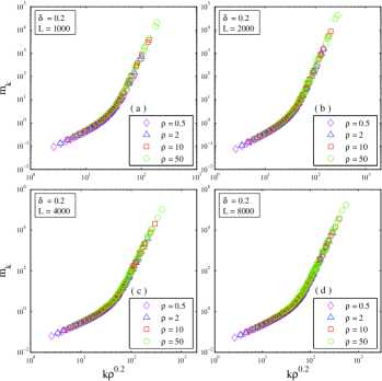
Figure 1: (Color online) The scaling relations of the average occupation number $m_{k}$ versus $k\rho^{\delta}$ at $\delta=0.2$ for different SF network sizes: (a) $L=1000$, (b) $L=2000$, (c) $L=4000$, (d) $L=8000$, at various densities $\rho=0.5$ (purple open diamonds), $\rho=2$ (blue open triangles), $\rho=10$ (red open squares), $\rho=50$ (green open circles), respectively.

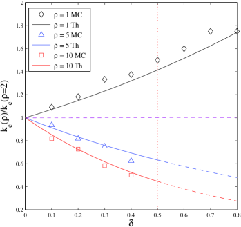
Figure 2: (Color online) The presence of the finite density effect in the crossover degree ratios $k_{c}(\rho)/k_{c}(\rho=2)$ versus the parameter $\delta$ with an SF network size $L=4000$, for various densities $\rho=1$ (black open diamonds and solid line), $5$ (blue open triangles and solid line), and $10$ (red open squares and solid line), respectively. The solid lines correspond to the theoretical calculation and the symbols to the MC simulation data. Note that $k_{c}$’s do not exist in regime $\delta>\delta_{c}$ ($\delta_{c}=0.5$ is the vertical red dotted dash line) for $\rho=5$ and $\rho=10$ due to the lower bound of degree $k_{\mathrm{min}}$, two theoretical dashed lines are only formally drawn in that region.

IV Finite Density Scaling Law of Relaxation Dynamics

The preceding theoretical predictions show that the occupation number distribution in the steady state is determined not only by the degree distribution $\mathscr{P}_{deg}(k)$ being independent of any other characteristics of underlying networks, but also the density of the particles hopping on the networks. However, the relaxation dynamics of ZRP is getting more complicated due to the effects of both the structure of underlying networks and the density.

So far only has a little been known about the dynamics of condensation in ZRP Godre03 ; Gross03 ; Godre17 . The finite density effects on the relaxation dynamics is hence one of the important issues to be addressed. In the following we only consider the case of $\delta<\delta_{c}$, in which a condensation phase transition occurs.we rely on the MC simulations and the scaling ansatz in order to understand the dynamical scaling properties.

Scaling ansatz is helpful for obtaining the qualitative features of relaxation dynamics. Previous studies Godre03 ; Gross03 revealed that, particles form macroscopic condensate by successive coarsening processes of the small clusters. The smaller clusters merge into larger ones, and grow until a single macroscopic condensate forms. The scaling hypothesis leads to the power-law growth of the relaxation time with the system size as $t_{R}\sim L^{\beta}$, where $\beta=1-\delta$ is the dynamic exponent.

The highly heterogeneous structure of SF networks deeply affect the relaxation dynamics of interacting particles system defined on them. It was hypothesized in Noh05a that the relaxation process follows some hierarchical dynamics. There exist two characteristic time-dependent degree scales $k_{\Omega c}(t)$ and $k_{\Omega}(t)$, which plays the role of the crossover degree $k_{c}$, and the role of $k_{max}$, respectively. During transient time $t$, a subnetwork of small degree nodes is equilibrated first and the equilibrated subnetwork keep expanding until $k_{\Omega}(t)$ grows in time and eventually reaches $k_{max}$.

It is natural to assume that a similar hierarchical dynamics occurs in a variable finite density situation. Starting from a fully random distribution at initial time, all particles behave as random walkers without interaction in a short period of time. Later on the distribution of particles further evolves and eventually approaches the steady state. Suppose there exist two characteristic degree scales in hierarchical relaxation dynamics. Those nodes with degree $k\leq k_{\Omega}$ consist of a smaller equilibrated subnetwork, denoted below by, say, $\Omega$, of size $L_{\Omega}<L$ in a transient time $t\ll t_{R}$, where $t_{R}$ is the relaxation time. Inside this subnetwork, the other characteristic degree $k_{\Omega\mathrm{c}}$ plays the role of crossover degree $k_{c}$ of the whole network. The equilibrated subnetwork keeps growing to proceed to the higher hierarchy until $k_{\Omega}$ reaches $k_{\mathrm{max}}$ of the network, the steady state of the ZRP is then formed. We may refer to those nodes with $k_{\Omega}$ as the temporary hub Noh05b . The average occupation number $m_{k_{\Omega}}$ versus the transient time $t$, according to the hierarchical dynamics, scales as

$$m_{k_{\Omega}}\sim\rho k_{\Omega}^{1/\delta_{c}}\sim t^{1/\nu}\,,$$ (34)

with $\nu=1-\delta$ being the dynamic exponent Noh05b . Clearly $k_{\Omega}$ evolves with time, however, we emphasize at this moment that $k_{\Omega}$ is also density dependent, i.e.,

$$k_{\Omega}\sim t^{\delta_{c}/\nu}/\rho^{\delta_{c}}\,.$$ (35)

We now turn to the other scale in the transient state: the crossover degree $k_{\Omega c}$. Just like $k_{c}$’s scaling in the steady state of the network, it scales as

$$k_{\Omega c}\sim k_{\Omega}^{1-\delta/\delta_{c}}/\rho^{\delta}\,,$$ (36)

and again, a density dependent factor $\rho^{-\delta}$ comes in.

The average occupation number of a node within the equilibrated network $m_{k}$ reads

$$m_{k}\sim\left\{\begin{array}[]{rl}\rho^{\delta}k/k^{1-\delta/\delta_{c}}_{\Omega},&\mbox{$k<k_{\Omega\mathrm{c}}$}\,,\\ \rho k^{1/\delta}/k^{1/\delta-1/\delta_{c}}_{\Omega},&\mbox{$k_{\Omega\mathrm{c}}<k<k_{\Omega}$}\,.\end{array}\right.$$ (37)

As a result, by applying Eq. (35), the scaling law of time- and density-dependent $m_{k}$ can be obtained as

$$m_{k}\sim\left\{\begin{array}[]{rl}k\rho^{\delta_{c}}/t^{(\delta_{c}-\delta)/\nu}\,,&\mbox{$k<k_{\Omega\mathrm{c}}$}\,,\\ (k\rho^{\delta_{c}})^{1/\delta}/t^{(\delta_{c}-\delta)/\delta\nu}\,,&\mbox{$k_{\Omega\mathrm{c}}<k<k_{\Omega}$}\,.\end{array}\right.$$ (38)

These explicit scaling laws of $m_{k}(t)$ versus $k\rho^{\delta_{c}}$ for some transient time $t$ can be unified in a single relation $m_{k}\sim\mathscr{H}(k\rho^{\delta_{c}})$, in which $\mathscr{H}$ is some scaling function, for given $t$ and $\delta$. MC simulations have to be performed to verify the above analytical predictions.

The results of MC simulations on the finite density effects of the relaxation dynamics are shown in Fig. 3(a). Note the different time scales involved in our relaxation dynamics simulations: the transient time scale $t$, the relaxation time scale $t_{R}$, the evolution time scale of the system $\tau$, and $t\ll t_{R}\ll\tau$. We took the evolution time $\tau=2^{20}$, which is long enough for system to evolve towards the steady state. The average occupation number $m_{k}(t)$ at transient time $t=2^{10}$, versus $k\rho^{\delta_{c}}$ with a given network size $L=4000$, but with various densities $\rho=0.5$ (purple open diamonds), $\rho=2$ (blue open triangles), $\rho=10$ (red open squares), and $\rho=50$ (green open circles), respectively, are shown.

As one can see from the left panel in the figure, the collapse of simulation data of $m_{k}$ w.r.t. $k\rho^{\delta_{c}}$ indicates the scaling law in the evolution of the relaxation for different densities. To understand the condensation dynamics, an appropriate characteristic order parameter is the infinity time limit of inverse participation ratio (IPR) $I_{t}$ Noh05a , which is defined as

$$I_{\infty}\equiv\lim_{t\rightarrow\infty}I_{t}=\lim_{t\rightarrow\infty}\frac{1}{N^{2}}\sum_{i=1}^{L}n^{2}_{i}(t)\,.$$ (39)

According to the hierarchical dynamics ansatz in condensation processes, the occupation number of particles on the temporary hub dominates in an equilibrated sub-network, note that the degree of the temporary hub $k_{\Omega}$ scales as $t^{\delta_{c}/\nu}/\rho^{\delta_{c}}$ as in Eq. (35), combining with $L_{\Omega}\sim k_{\Omega}^{1/\delta_{c}}$, the size of the equilibrated sub-network satisfies $L_{\Omega}\sim t/\rho^{\nu}$ for a given transient time $t$. Hence the IPR ratio, describing the extent of condensation for a given network size $L$, possesses the same scaling relation $I_{t}/I_{\infty}\sim t/\rho^{\nu}$, while for the long run $\tau\gg t_{R}$ the steady state is reached and the particles on the hub dominate.

In Fig. 3(b), we plot the scaling relations of $I_{t}/I_{\infty}$ versus $t/\rho^{\nu}$ at $\delta=0.2$ for $\rho=0.5$, $\rho=2$, $\rho=10$, and $\rho=50$, respectively. A total $\tau=2^{20}$ time-step evolution has been fulfilled to ensure the realization of the steady state, i.e., $I_{\tau}\rightarrow I_{\infty}$. One immediately sees that the increasing density naturally postpones the occurrence of the condensation transition, and the collapse of data of different densities nicely confirms our prediction.

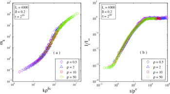
Figure 3: (Color online) Data collapse plot of (a) the average occupation number $m_{k}$ versus $k\rho^{\delta_{c}}$ at the transient time $t=2^{10}$, (b) the evolution of ratio of IPR to its steady state limit, $I_{t}/I_{\infty}$, versus $t/\rho^{\nu}$, with $\nu={1-\delta}$ being the dynamic exponent in the relaxation dynamics, at $\delta=0.2$ for network size $L=4000$, and various densities $\rho=0.5$ (purple open diamonds), $\rho=2$ (blue open triangles), $\rho=10$ (red open squares), and $\rho=50$ (green open circles), respectively.

V Summary

In summary, we explored the finite density effects on both the steady and dynamical properties of the ZRP on SF network with hopping rate function $u(n)=n^{\delta}$. By means of the GCE method, we discovered that the steady state condensation phase transition is driven not only by the disorder of the underlying SF network, but also by the finite density of the interacting particles. The crossover degree $k_{c}$ and the average occupation number $m_{k}$ were found to be both density dependent, and satisfy the corresponding scaling laws. In contrast to the ZRP on SF network with fixed density, the ratios of the crossover degree $k_{c}$ for two different densities at given size of network exhibit a non-constant behavior.

The influences of the density on the relaxation dynamics was also analytically investigated. The hierarchical characteristics of the relaxation dynamics renders the process proceeding from nodes with lower degrees toward those with higher degrees. With the help of the scaling ansatz, the scaling laws of the condensation transition (to the steady state) were predicted. At a specific time $t\ll t_{R}$ the average occupation number scales as $m_{k}\sim k\rho^{\delta_{c}}$ for various densities. The evolution of the ratio of IPR to its steady state limit follows a scaling law $I_{t}/I_{\infty}\sim t/\rho^{\nu}$ with dynamical exponent $\nu=1-\delta$. To verify our analytically derived scaling laws, we have performed the Monte Carlo simulations for varied densities. The corresponding scaling relations are validated very well by numerical experiments.

- (1) See, e.g., M. H. Anderson, J. R. Ensher, M. R. Matthews, C. E. Wieman, and E. A. Cornell, Science 269, 198 (1995); K. B. Davis, M.-O. Mewes, M. R. Andrews, N. J. van Druten, D. S. Durfee, D. M. Kurn, and W. Ketterle, Phys. Rev. Lett. 75,3969 (1995); C. C. Bradley, C. A. Sackett, J. J. Tollett, and R. G. Hulet, Phys. Rev. Lett. 75, 1687 (1995).
- (2) D. Chowdhury, L. Santen, and A. Schadschneider, Phys. Rep. 329, 199 (2000).
- (3) D. van der Meer, K. van der Weele, and D. Lohse, Phys. Rev. Lett. 88, 174302 (2002).
- (4) D. van der Meer, K. van der Weele, and D. Lohse, J. Stat. Mech. Theor. Exp. 04, P 04004 (2004).
- (5) P. L. Krapivsky, S. Redner, and F. Leyvraz, Phys. Rev. Lett. 85, 4629 (2000).
- (6) G. Bianconi and A.-L. Barabási, Phys. Rev. Lett. 86, 5632 (2001).
- (7) G. Su, X. Zhang and Y. Zhang, Euro. Phys. Lett. 100, 38003 (2012).
- (8) R. K. Pathria and P. D. Beale, Statistical Mechanics, 3rd. ed. (Academic Press, 2011).
- (9) T. M. Liggett, Stochastic interacting systems: contact, voter, and exclusion processes (Springer Berlin, 1999).
- (10) B. Schmittmann and R. K. P. Zia, Statistical Mechanics of Driven Diffusive Systems, ed. C. Domb and J. L. Lebowitz (Academic Press, New York, 1995)
- (11) M. R. Evans, Y. Kafri, H. M. Koduvely, and D. Mukamel, Phys. Rev. Lett. 80, 425 (1998).
- (12) M. R. Evans, T. Hanney, and S. N. Majumdar, Phys. Rev. Lett. 97, 010602 (2006).
- (13) F. Spitzer, Adv. Math. 5, 246 (1970).
- (14) M. R. Evans and T. Hanney, J. Phys. A: Math. Gen. 38, R195 (2005).
- (15) C. Godrèche, Lect. Notes Phys. 716, 261 (2007).
- (16) M. R. Evans, Braz. J. Phys. 30, 42 (2000).
- (17) S. Großkinsky, G. M. Schütz, and H. Spohn, J. Stat. Phys. 113, 389 (2003).
- (18) S. N. Majumdar, M. R. Evans, and R. K. P. Zia, Phys. Rev. Lett. 94, 180601 (2005).
- (19) C. Godrèche, and J. M. Luck, J. Stat. Mech. P12013 (2012).
- (20) R. Albert and A.-L. Barábasi, Rev. Mod. Phys. 74, 47 (2002).
- (21) V. M. Eguiluz, D. R. Chialvo, G. A. Cecchi, M. Baliki, and A. V. Apkarian, Phys. Rev. Lett. 94, 018102 (2005).
- (22) S. Boccaletti, V. Latora, Y. Moreno, M. Chavez, and D.-U. Hwang, Phys. Rep. 424, 175 (2006).
- (23) A.-L. Barabási and R. Albert, Science 286, 509 (1999); A.-L. Barabási, R. Albert, and H. Jeong, Physica A 272, 173 (1999).
- (24) A. V. Goltsev, S. N. Dorogovtesev, and J. F. F. Mendes, Rev. Mod. Phys. 80, 1275 (2008).
- (25) M. Barthelemy, A. Barrat, R. Pastor-Satorras, and A. Vespignani, Phys. Rev. Lett. 92, 178701 (2004).
- (26) V. Sood and S. Redner, Phys. Rev. Lett. 94, 178701 (2005).
- (27) J. D. Noh, G. M. Shim, and H. Lee, Phys. Rev. Lett. 94, 198701 (2005).
- (28) J. D. Noh, Phys. Rev. E 72, 056123 (2005).
- (29) M. Tang, Z. Liu, and J. Zhou, Phys. Rev. E 74, 036101 (2006).
- (30) R. Cohen, K. Erez, D. ben-Avraham, and S. Havlin, Phys. Rev. Lett. 85, 198701 (2000).
- (31) J. D. Noh and H. Rieger, Phys. Rev. Lett. 92, 118701 (2004).
- (32) J. Krug and P. A. Ferrari, J. Phys. A 29, L465 (1996); J. Krug, Braz. J. Phys. 30, 97 (2000).
- (33) M. R. Evans, Europhys. Lett. 36, 13 (1996).
- (34) K. Jain and M. Barma, Phys. Rev. Lett. 91, 135701 (2003).
- (35) M. R. Evans, S. N. Majumdar, and R. K. P. Zia, J. Phys. A 37, L275 (2004).
- (36) R. K. P. Zia, M. R. Evans, and S. N. Majumdar, J. Stat. Mech.: Theor. Exp. L10001 (2004).
- (37) C. Godrèche, J. Phys. A: Math. Theor. 36 6313 (2003).
- (38) S. Großkinsky, and T. Hanney, Phys. Rev. E 72, 016129 (2005).
- (39) C. Godrèche and J. M. Drouffe, J. Phys. A: Math. Theor. 50, 015005 (2017).