A Theory of Nonlinear Signal-Noise Interactions in Wavelength Division Multiplexed Coherent Systems

Abstract

a general theory of nonlinear signal-noise interactions for wavelength division multiplexed fiber-optic coherent transmission systems is presented. This theory is based on the regular perturbation treatment of the nonlinear Schrödinger equation, which governs the wave propagation in the optical fiber, and is exact up to the first order in the fiber nonlinear coefficient. It takes into account all cross-channel nonlinear four-wave mixing contributions to the total variance of nonlinear distortions, dependency on modulation format, erbium-doped fiber and and backward Raman amplification schemes, heterogeneous spans, and chromatic dispersion to all orders; moreover, it is computationally efficient, being 2-3 orders of magnitude faster than the available alternative treatments in the literature. This theory is used to estimate the impact of signal-noise interaction on uncompensated, as well as on nonlinearity-compensated systems with ideal multi-channel digital-backpropagation.

I Introduction

The spectral efficiency of fiber-optic wavelength division multiplexed (WDM) transmission systems is fundamentally limited by intra- and inter-channel four-wave mixing (FWM) processes stemming from the optical fiber intensity-dependent nonlinear Kerr refractive index [1, 2]. Many of the recent high-capacity ultra long-haul “hero experiments” exploited single-channel digital nonlinear compensation (NLC) to deal with fiber nonlinear impairments and to push the transmission limits imposed by such FWM terms [3, 4, 5, 6, 7, 8, 9, 10].

The propagation of the perfectly polarized electromagnetic field in the optical fiber is modeled by the nonlinear Schrödinger equation (NLS). In order to account for the random birefringence in fiber optics, it is common to use the Manakov approximation of the system of two coupled NLS equations governing the transverse components of the total electromagnetic field[1].

Since 2010, much progress has been made in developing analytical models for polarization-multiplexed (PM) WDM coherent transmission systems. These models have been proved to be particularly successful in predicting the performance of dispersion un-managed (DU) systems, and have been validated numerically and experimentally many times by various groups. (for instance cf. [11]). Most of these analytical models are based on the regular perturbation (RP) approximation of the solutions of NLS and/or Manakov equation, where only terms up to the first-order in fiber nonlinear coefficient are kept.

The first attempts in developing a complete theory of nonlinear propagation in the modern coherent PM-WDM DU systems, by Chen, Poggiolini and Carena, resulted in the so-called Gaussian noise model (GNM)[12, 13, 14, 15]. An independent derivation was published by Johannisson and Karlsson [16]. In the GNM, the WDM signal is modeled as a Gaussian random process all along the link, i.e., from the injection point into fiber at the transmitter side up to the receiver side front-end. This Gaussian random process is represented as a grid of Dirac delta functions in the frequency domain at the channel input. The amplitude of each delta function is modulated by a Gaussian random variable. All FWM terms among these spectral lines are then computed at channel output, and finally the power spectral density (PSD) of the nonlinear distortions, considered as additive Gaussian noise in absence of nonlinear compensation, is computed. The GNM relies on the hypothesis that large accumulated dispersions scramble the symbols such that according to the central limit theorem, sampled signal’s probability density function at the receiver tends to a circular complex Gaussian distribution per polarization, independent of the modulation format; therefore, The domain of validity of GNM is limited as the modulation-dependent contributions are absent, and the low-dispersion regime cannot be modeled.

The second approach was laid down in a seminal paper by Mecozzi and Essiambre, [17], where the RP method was rigorously applied to the equivalent nonlinear fiber channel comprising the multi-span amplified fiber-optic link and the matched-filtered sampled ideal coherent receiver. This work was based on the pioneering work of Mecozzi in 2000 [18], where the FWM of optical Gaussian pulses in an optical fiber was rigorously studied for the first time. The main result of this work is computing the third-order time-domain Volterra series coefficients of the equivalent nonlinear fiber channel, which are sufficient to exactly express nonlinear distortions up to the first-order of fiber nonlinear coefficient. Based on [17], a general more accurate theory of nonlinear impairments was developed by Dar [19, 20, 21, 22], where the impact of modulation format was properly taken into account, and the passage to the high dispersion regime is no more a requirement. He was able to transform the summation over the magnitude square of all Volterra coefficients, which is necessary to obtain the variance of the nonlinear impairments when considered as noise, into equivalent integral representations, and then efficiently compute those integrals by standard Monte Carlo sampling. Following this work, the GNM was upgraded to the enhanced Gaussian noise model (EGN) [23]. Recently, the full second-order statistics of the nonlinear impairments, i.e., not just the variance, but the whole autocorrelation of the nonlinear distortions was computed[24].

The third approach, also inspired by[17], as well as[25], was suggested by Serena and Bononi [26, 27], where they proposed to consider the evolution of the time-domain autocorrelation function of the nonlinear distortions along the fiber-optic link. The dependence on modulation formats, and dispersion management could be taken into account. Monte Carlo simulations are necessary to compute the propagation of the autocorrelation function along the link.

All the above-mentioned works only addressed FWM processes among signal waves. They did not account for the FWM between the signal and the co-propagating distributed noise waves injected by the optical amplifiers along the link, sometimes referred to as nonlinear signal-noise interaction (NSNI). Developing a rigorous theory for NSNI is important for at least two reasons: first, it can accurately quantify the amount by which the performance is degraded in various system configurations, (i.e., for different symbol rates, modulation formats, channel spacings, channel counts, number of spans, dispersion maps, fiber types, amplification schemes, etc.); second, it can contribute to answering the questions regarding the fundamental limits of performance improvements provided by nonlinear compensation (NLC).

The two most studied digital NLC algorithms are the digital backpropagation (DBP) [28, 29], and the less complex, but less accurate perturbation-based NLC (PNLC) [30], [31], which is based on the theoretical analysis in[17, 18]. The performance of the single-channel NLC, where only the intra-channel nonlinear impairments are partially equalized, either by DBP or by PNLC, is limited by the cross-channel nonlinear interference (NLI)[32]. Recently many researchers have investigated multi-channel DBP [33, 34, 35, 36, 37, 38]. In the absence of stochastic fluctuations due to distributed noise, or random birefringence, NLS and Manakov equations have space-reversal symmetry, thus zero-forcing (ZF) full-field equalization by DBP fully compensates the nonlinear fiber channel. On the other hand, the presence of NSNI, and/or polarization effects in the channel breaks the space-reversal symmetry, consequently full-field DBP equalization gain is reduced. It is important to assess the achievable signal-to-noise ratio (SNR) improvement due to multi-channel DBP in presence of real irreversible physical phenomena like NSNI and or random polarization effects, in order to determine the fundamental limits of information transmission in optical fibers, and in order to compare multi-channel DBP with other NLC techniques that are currently being investigated, most importantly, optical phase conjugation[40] and nonlinear Fourier transform [41, 42]. The theory presented in this work contributes to answering the questions regarding the constraints imposed on multi-channel DBP by NSNI.

The interaction between signal and noise in nonlinear optics has been studied since 1960’s. Since 2010, a few authors studied NSNI in the context of modern coherent fiber-optic transmission systems. Ref. [43] presents a complete numerical investigation of various nonlinear impairments in coherent and non-coherent dispersion-managed (DM) systems, with OOK, BPSK and QPSK formats, where, for each scenario the dominant nonlinear impairment is identified. The impact of NSNI on the performance degradation of DBP for 100G coherent PDM-QPSK systems is studied in[33] by numerical simulations. Ref.[44] investigates NSNI in 100G coherent systems for both DU and DM systems, both numerically and experimentally, and shows that dispersion management significantly enhances the degrading effect of NSNI. The impact of PMD on NSNI in 100G coherent systems is studied in[45] by means of numerical simulations. The first theoretical treatment of NSNI for coherent transmission systems is presented in[46], where a discrete channel model is introduced to calculate the impact of NSNI on the performance of single-channel coherent DU systems either without or with DBP, but the derivations are based on many simplifying assumptions. Ref.[47] numerically examines NSNI-induced system reach degradations, which in some cases amount to 15-20% in DU PDM-QPSK transmissions, and demonstrates that this reach degradation can be explained by a simple phenomenological modification of the GNM, by taking into account signal depletion by noise. The first detailed model of NSNI for coherent systems, is by Serena[48], which is based on [27]. The variance of the NSNI is computed by propagating the autocorrelation of nonlinear distortions along the link by means of numerical simulations. DBP can be included in the analysis. Although this approach is general, the numerical computations necessary to calculate the evolution of the autocorrelation functions are still time consuming.

In this paper, we present a general theory of NSNI for coherent WDM transmission systems, which is exact up to the first-order in fiber nonlinear coefficient, assuming RP, and has the advantage that it is 2-3 orders of magnitude faster than the approach proposed in[48]. Although perturbation approximations other than RP have been used to deal with nonlinear effects in the fiber-optic systems[49], we adopt RP in this work, as the previously discussed analytical treatments of fiber nonlinearity for modeling signal-signal FWM in coherent WDM transmission systems, which are all based on RP, have been proved to be adequate in practice. Our derivation is based on[17], and the summation technique introduced in [19, 20, 21, 22]. The theory developed here applies to both DM and DU systems, with heterogeneous spans, and both EDFA and Raman amplification schemes. It can deal with chromatic dispersion to all orders; however, the explicit formulas we present in the last sections only include the second-order dispersion, which is to avoid a too cumbersome presentation. The implications of higher order chromatic dispersion terms beyond the second-order is left for future (cf.[16] for a discussion of the impact of the third-order dispersion on signal-signal nonlinear distortions). We will then use the developed theory to compute the SNR for systems compensated by ideal multi-channel DBP. This computation is useful in providing an estimate on the achievable information rate with ideal ZF DBP compensation. We do not address more sophisticated nonlinear equalization schemes like stochastic DBP[50]. The paper is organized as follows. In section II we present the preliminary materials; the notation is introduced, and the basic equations describing the transmitted signal, channel, and the coherent receiver are written down. In section III we present the first-order regular perturbation theory of WDM propagation, containing both signal-signal and signal-noise FWM contributions. Section V concludes the paper. The detailed derivation of the integrals that appear in the expressions of the formulas for the variance of nonlinear distortions, as well as efficient numerical integration technique to compute those integrals are discussed in the appendix.

II Preliminaries

In this section we give an exact mathematical description of the multi-span WDM coherent fiber-optic transmission systems, which is the subject of the investigation of this paper. In II.A we define the basic notations and remind some mathematical relations that will be frequently used in the later derivations. In II.B we describe the multi-span single-polarization optically-amplified fiber-optic channel model based on NLS. We assume that noisy erbium-doped fiber amplifiers (EDFA) are placed at the end of each span. We assume heterogeneous spans, with position-dependent dispersion and loss coefficients, so, if necessary, dispersion management, and/or backward Raman amplification can be included in the analysis. The NLS is transformed to a normalized NLS, derived with amplified spontaneous emission (ASE) noise process, and also with the third-order nonlinear term scaled by an effective power profile. The impact of signal depletion by ASE noise is exactly accounted for in deriving the power profile, and the spatio-temporal autocorrelation function of ASE is calculated. In II.C, we describe the ideal matched-filtered coherent receiver, with ideal front-end, and where symbol-by-symbol detection is assumed and no digital signal processing, except for matched filtering, is applied. All the developments in this and the subsequent sections are for perfectly polarized electromagnetic field and NLS. The extension to double polarization and Manakov equation is made in III.H. The notation introduced in this section is faithful to that of [17].

II-A Notations and basic definitions

We start by reviewing a few relations and introducing some notational devices that prove to be useful in the sequel. In this work we are dealing with stochastic processes that are functions of propagation distance $z$ and time $t$. The randomness is due to information symbols and amplifier noise. Let’s denote a sample waveform by $x(z,t)$. The Fourier transform pair is

$$\tilde{x}\left({z,\omega}\right)=\mathcal{F}\left[{x\left({z,t}\right)}\right]=\int_{-\infty}^{+\infty}{dt\exp\left({i\omega t}\right)x\left({z,t}\right),}$$ (1)

$$x\left({z,t}\right)={\mathcal{F}^{-1}}\left[{\tilde{x}\left({z,\omega}\right)}\right]=\frac{1}{{2\pi}}\int_{-\infty}^{+\infty}{d\omega\exp\left({-i\omega t}\right)\tilde{x}\left({z,\omega}\right),}$$ (2)

where, $\mathcal{F}$ stands for Fourier transform, $\mathcal{F}^{-1}$ stands for inverse Fourier transform, $\omega=2\pi f$ is the angular frequency, and $f$ is the frequency. Throughout this paper, a waveform with a tilde on top is the Fourier transform of the waveform denoted by the same symbol but without tilde. We have:

$$\mathcal{F}\left[{x\left({z,t-{t_{0}}}\right)}\right]=\exp\left({+i\omega{t_{0}}}\right)\tilde{x}\left({z,\omega}\right),$$ (3)

$$\mathcal{F}\left[{\exp\left({-i{\omega_{0}}t}\right)x\left({z,t}\right)}\right]=\tilde{x}\left({z,\omega-{\omega_{0}}}\right),$$ (4)

and

$$\mathcal{F}\left[{\exp\left({-i{\omega_{0}}t}\right)x\left({z,t-{t_{0}}}\right)}\right]=\\ \exp\left[{i\left({\omega-{\omega_{0}}}\right){t_{0}}}\right]\tilde{x}\left({z,\omega-{\omega_{0}}}\right).$$ (5)

In this work we consider only the second-order group velocity dispersion (GVD) for simplicity, but, if necessary, higher order dispersion terms can be included in the analysis without posing any problem. We introduce the following notation for the dispersion operator in frequency domain

$${\hat{\mathcal{D}}_{z^{\prime}}}\left[{\tilde{x}\left({z,\omega}\right)}\right]={\exp\left({i\frac{{{\omega^{2}}}}{2}}{\int_{0}}^{z^{\prime}}dz^{\prime\prime}{\beta_{2}}(z^{\prime\prime})\right)}\tilde{x}\left({z,\omega}\right),$$ (6)

and in the time domain

$${\hat{\mathcal{D}}_{z^{\prime}}}\left[{x\left({z,t}\right)}\right]=\\ {\mathcal{F}^{-1}}\left[{\exp\left({i\frac{{{\omega^{2}}}}{2}}{\int_{0}}^{z^{\prime}}dz^{\prime\prime}{\beta_{2}}(z^{\prime\prime})\right)\tilde{x}\left({z,\omega}\right)}\right].$$ (7)

Note that, for simplicity, we use the same notation for the dispersion operator, notwithstanding whether it is applied to a frequency-domain signal, as per (6), or to a time-domain signal, as per (7). Given the context, this should not cause any ambiguity. We define the following notations for waveforms crosscorrelations in time domain

$$\left\langle{x\left({z,t}\right),y\left({z^{\prime},t^{\prime}}\right)}\right\rangle=\int_{-\infty}^{+\infty}{d\tau}{x^{*}}\left({z,t+\tau}\right)y\left({z^{\prime},t^{\prime}+\tau}\right),$$ (8)

and in frequency domain

$$\left\langle{\tilde{x}\left({z,\omega}\right),\tilde{y}\left({z^{\prime},\omega^{\prime}}\right)}\right\rangle=\int_{-\infty}^{+\infty}{d\nu}{\tilde{x}^{*}}\left({z,\omega+\nu}\right)\tilde{y}\left({z^{\prime},\omega^{\prime}+\nu}\right),$$ (9)

where, the superscript $*$ stands for complex conjugation. On the other hand, we use the notation $\left\langle{x\left({z,t}\right)}\right\rangle$ to denote the ensemble average over the space of all sample waveforms of the stochastic process $x(z,t)$. The randomness of the processes in this work is due to information symbols, which are assumed to be independent identically distributed (i.i.d.) discrete random variables with phase-isotropic distributions, and also due to amplifier noise.

In our notation, the Parseval’s theorem is stated as follows

$$\left\langle{x\left({z,t}\right),y\left({z^{\prime},t}\right)}\right\rangle=\frac{1}{{2\pi}}\left\langle{\tilde{x}\left({z,\omega}\right),\tilde{y}\left({z^{\prime},\omega}\right)}\right\rangle.$$ (10)

The following dispersion exchange formula (DEF), which is easily proven by Parseval’s theorem, will be extensively used in this work:

$$\left\langle{x\left({z,t}\right),{{\hat{\mathcal{D}}}_{z^{\prime}}}\left[{y\left({z,t}\right)}\right]}\right\rangle=\left\langle{{{{\hat{\mathcal{D}}}^{\dagger}}_{z^{\prime}}}\left[{x\left({z,t}\right)}\right],y\left({z,t}\right)}\right\rangle,$$ (11)

where, $\hat{\mathcal{D}}^{{\dagger}}_{z^{\prime}}$ is the adjoint of the dispersion operator $\hat{\mathcal{D}}_{z^{\prime}}$, which is defined to be

$${{\hat{\mathcal{D}}^{\dagger}}_{z^{\prime}}}\left[{\tilde{x}\left({z,\omega}\right)}\right]={\exp\left(-{i\frac{{{\omega^{2}}}}{2}}{\int_{0}}^{z^{\prime}}dz^{\prime\prime}{\beta_{2}}(z^{\prime\prime})\right)}\tilde{x}\left({z,\omega}\right).$$ (12)

All waveforms are assumed to be base-band analytical signals. We use the first subscript for continuous waveforms to denote time-shifts by multiples of symbol duration, i.e.,

$${x_{k}}\left({z,t}\right)=x\left({z,t-{T_{k}}}\right),$$ (13)

where, $T_{k}=kT$, $T$ is the symbol duration and $k$ is an arbitrary integer. When used to decorate a discrete random variable, the first subscript $k$ denotes the $k$’th symbol. The second subscript, both for continuous waveforms, and for discrete random variables, denotes the WDM channel index. Thus $a_{k,s}$ denotes the $k$’th symbol of the $s$’th channel, and $x_{k,s}(z,t)$ denotes the base-band waveform of the $s$’th channel time shifted by $kT$. The channel of interest (COI) is indexed $s=0$. If the second index is zero it can be optionally dropped in order to simplify the notation, therefore: $a_{k}=a_{k,0}$, and $x_{k}(z,t)=x_{k,0}(z,t)$. The total optical field at distance $z$ and time $t$ is denoted by $E(z,t)$. The total optical field at fiber input ($z=0$) is written as

$$E\left({0,t}\right)=\sum\limits_{k}{{a_{k}}{A_{k}}\left({0,t}\right)}+\\ \sum\limits_{k,s\neq 0}{{a_{k,s}}{A_{k,s}}\left({0,t-\delta{T_{s}}}\right)\exp\left[{-i{\Omega_{s}}t+i{\phi_{s}}\left(0\right)}\right]},$$ (14)

where, as mentioned above, $a_{k}$ is the $k$’th symbol of the COI, $a_{k,s}$ is the $k$’th symbol of the $s$’th adjacent channel, $\Omega_{s}$ is the center frequency detuning of the $s$’th adjacent channel with respect to COI, $\delta T_{s}$ is the time offset of the $s$’th adjacent channel with respect to COI, $\phi_{s}(0)$ is the initial, i.e., $z=0$, phase offset of the $s$’th adjacent channel with respect to COI, $A_{0}(0,t)$ is the pulseshape of the COI, and $A_{0,s}(0,t)$ is the pulseshape of the $s$’th channel. In this work, we suppose that $A_{0,s}(0,t)=A_{0}(0,t)$ for all $s$. The energy, $\mathcal{E}$, of the pulseshapes is given by the following integral

$$\mathcal{E}=\int_{-\infty}^{+\infty}{{{\left|{{A_{0}}\left({0,t}\right)}\right|}^{2}}dt}.$$ (15)

The normalized pulseshape is defined as

$${U_{0}}\left({0,t}\right)=\frac{{{A_{0}}\left({0,t}\right)}}{{\sqrt{\mathcal{E}}}}.$$ (16)

In this work we w assume Nyquist pulse-shaping is applied to all channels. As a consequence, the following orthogonality relation holds for the pulses

$$\left\langle{{A_{k}}\left({0,t}\right),{A_{h}}\left({0,t}\right)}\right\rangle={\mathcal{E}}{\delta_{hk}},$$ (17)

which is equivalent to the following orthonormality condition for the normalized pulses

$$\left\langle{{U_{k}}\left({0,t}\right),{U_{h}}\left({0,t}\right)}\right\rangle={\delta_{hk}},$$ (18)

where, $\delta_{hk}$ is the Kronecker delta function.

II-B Nonlinear Schrödinger equation (NLS)

If polarization effects are ignored, the total optical field satisfies the the NLS, i.e.,

$${\partial_{z}}E=\frac{{g\left(z\right)-\alpha(z)}}{2}E-i\frac{{{\beta_{2}(z)}}}{2}\partial_{t}^{2}E+i\gamma(z){\left|E\right|^{2}}E+n\left({z,t}\right),$$ (19)

where, $g(z)$ is the local power gain coefficient, $\alpha(z)$ is the local fiber attenuation coefficient, $\beta_{2}(z)$ is the local GVD coefficient, $\gamma(z)$ is the local fiber nonlinear Kerr coefficient, and $n(z,t)$ is the amplified spontaneous emission (ASE) noise source. Let’s denote the COI wavelength by $\lambda_{0}$. The measured channel carrier angular frequency is $\omega_{0}=2\pi c/\lambda_{0}$, where $c$ is the speed of light. Note that, $\gamma=2\pi n_{2}/\lambda_{0}A_{eff}$, where $n_{2}$ is the fiber nonlinear Kerr refractive index, and $A_{eff}$ is the fiber effective area.

In writing (19) we assumed that the local power gain coefficient is frequency-independent, i.e.,

$$g\left({z,{\omega}}\right)=g\left({z,{\omega_{0}}}\right)=g\left(z\right).$$ (20)

The frequency-independent local power gain coefficient can be explicitly written as

$$g\left(z\right)=\sum\limits_{n=1}^{{N_{s}}}{{g_{n}}\delta\left({z-{z_{n}}}\right)},$$ (21)

where, $\delta(\cdot)$ is the Dirac delta function, $g_{n}$ is the local gain coefficient of the EDFA placed at the end of the $n$’th span, $N_{s}$ is the total number of spans, and $z_{n}$ is the coordinate of the end of the $n$’th span. We also define

$$z_{0}=0.$$ (22)

The ASE noise source in (19) is a complex circular Gaussian random process with zero mean and the following time-domain autocorrelation function

$$\left\langle{{n^{*}}\left({z,t}\right)n\left({z^{\prime},t^{\prime}}\right)}\right\rangle=C\left({z,t-t^{\prime}}\right)\delta\left({z-z^{\prime}}\right).$$ (23)

The Fourier transform of the noise source autocorrelation, i.e., the space-dependent power spectral density of the ASE source is

$$\left\langle{{{\tilde{n}}^{*}}\left({z,\omega}\right)\tilde{n}\left({z^{\prime},\omega^{\prime}}\right)}\right\rangle=2\pi\tilde{C}\left({z,\omega}\right)\delta\left({z-z^{\prime}}\right)\delta\left({\omega-\omega^{\prime}}\right),$$ (24)

where, we have

$$\tilde{C}(z,\omega)=\hbar\omega_{0}\sum\limits_{n=1}^{{N_{s}}}{{g_{n}}{n_{\text{sp},n}}(\omega)\delta(z-z_{n})},$$ (25)

where, $n_{\text{sp},n}(\omega)$ is the noise figure of the $n$’th amplifier, and $\hbar$ is Planck’s constant divided by $2\pi$.

Now, in order to simplify further developments, we derive a normalized version of NLS by factoring out the power profile. Let’s define the normalized total optical field $U(z,t)$ as follows

$$E\left({z,t}\right)=\Psi\left(z\right)U\left({z,t}\right),$$ (26)

where, the power envelop function $\Psi(z)$ satisfies the following equation by definition

$$\frac{d}{{dz}}\Psi\left(z\right)=\frac{{g\left(z\right)-\alpha(z)}}{2}\Psi\left(z\right),$$ (27)

with the initial condition

$$\Psi\left(0\right)=\sqrt{\mathcal{E}}.$$ (28)

Now, we define the normalized power profile function $f(z)$ as

$$f(z)=\frac{1}{\sqrt{\mathcal{E}}}\Psi(z).$$ (29)

We can solve (27) and apply the initial condition (28) and the definition (29) to obtain

$$f\left(z\right)=\exp\left\{{\int_{0}^{z}{dz^{\prime}\left[{g\left({z^{\prime}}\right)-\alpha\left({z^{\prime}}\right)}\right]}}\right\}.$$ (30)

After substituting (26) into (19) and using (27) and (29), we can derive the following normalized NLS

$${\partial_{z}}U=-i\frac{{{\beta_{2}(z)}}}{2}\partial_{t}^{2}U+i{\mathcal{E}}\gamma(z)f\left(z\right){\left|U\right|^{2}}U+\frac{{n\left({z,t}\right)}}{{\sqrt{{\mathcal{E}}f\left(z\right)}}},$$ (31)

In this work, for simplicity, we assume that all channels have the same average launch power per channel, which is denoted by $P$; we have

$${P}=\frac{\mathcal{E}}{T};$$ (32)

Moreover, we assume that all EDFAs operate in the constant output power mode. Let’s denote the ASE power at the output of the $n^{\text{th}}$ EDFA, i.e., the EDFA placed at the end of the $n^{\text{th}}$ span, by $N_{n}$, and the optical power transferred from the $(n-1)^{\text{th}}$ span to the $n^{\text{th}}$ span, after amplification by the $n^{\text{th}}$ EDFA, by $S_{n}$. We have

$$\begin{array}[]{*{20}{c}}{N_{n}=(e^{g_{n}}-1)\sigma_{n}^{2}}&{n=1,\ldots,{N_{s}}},\end{array}$$ (33)

where

$$\sigma_{n}^{2}=\hbar\omega_{0}\int_{-\infty}^{+\infty}{d\omega n_{\text{sp},n}}(\omega).$$ (34)

Note that $N_{0}=0$, and $S_{0}=P$. We have

$$\begin{array}[]{*{20}{c}}{S_{n}=e^{g_{n-1}-l_{n-1}}(S_{n-1}+N_{n-1})}&{n=1,\ldots,{N_{s}}},\end{array}$$ (35)

where, the $l_{n}$ is the loss exponent of the $n^{\text{th}}$ span, which is

$${l_{n}}=\int_{{z_{n-1}}}^{{z_{n}}}{dz\alpha\left(z\right)}.$$ (36)

The constant output power assumption for EDFAs amounts to

$$\begin{array}[]{*{20}{c}}{{S_{n}}+{N_{n}}={P}}&{n=1,\ldots,{N_{s}}}.\end{array}$$ (37)

Note that the noise figure function $n_{\text{sp},n}(\omega)$ is dimensionless; therefore, the noise variance $\sigma_{n}^{2}$ in (34) has the dimension of power. Now, let’s define the following dimensionless parameter

$${\zeta_{n}}=\frac{{\sigma_{n}^{2}}}{{{P}}},$$ (38)

as well as

$${d_{n}}={l_{n}}-{g_{n}},$$ (39)

where, the $d_{n}$ is the signal gain depletion exponent in the $n^{\text{th}}$ by the ASE power generated at that span. Using (33), (35), (37), (38), and (39), we have

$$d_{n}=\ln(\frac{1+e^{l_{n}}\zeta_{n}}{1+\zeta_{n}}),$$ (40)

where $n=1,\ldots,N_{s}$. We also define

$$d_{0}=0.$$ (41)

The accumulated signal depletion exponent is denoted by $\delta_{n}$, and is given by

$${\delta_{n}}=\sum\limits_{m=0}^{n}{{d_{m}}}.$$ (42)

Using these definitions we find the following expression for the normalized power profile

$$f\left(z\right)=\begin{array}[]{*{20}{c}}{\exp\left[{-{\delta_{n-1}}-\int_{{z_{n-1}}}^{z}{dz^{\prime}\alpha\left({z^{\prime}}\right)}}\right],}&{{z_{n-1}}\leq z<{z_{n}}},\end{array}$$ (43)

for ${n=1,\ldots,{N_{s}}}$. This expression for the normalized power profile is general, in that spans with arbitrary length and loss coefficients can be modeled, the noise figure of the EDFAs are different; moreover, backward Raman amplification can be modeled by properly defining a $z$-dependent loss coefficient function $\alpha(z)$. Finally note that, in order to model the system when the EDFAs operate in the constant gain mode, we only need to force $d_{n}=0$ for $n=0,\ldots,N_{s}$.

II-C Coherent Receiver

We assume ideal matched-filter symbol-by-symbol coherent receiver. The total transmission distance is denoted by $L$. The impulse response of the matched filter is denoted by $u_{f}(t)$. We have

$${u_{f}}\left(t\right)={{D_{0}}^{*}}\left({-t}\right),$$ (44)

where,

$${D_{0}}\left(t\right)={{\hat{\mathcal{D}}}_{L}}\left[{{U_{0}}\left({0,t}\right)}\right].$$ (45)

The photocurrent at the output of the matched filter is denoted by ${\mathcal{I}}$, and is given by the following equation

$${\mathcal{I}}\left(t\right)={u_{f}}\left(t\right)\otimes U\left({L,t}\right),$$ (46)

where, the symbol $\otimes$ stands for the convolution operation in time domain. The sampled photocurrent at time $t=kT$ is

$${\mathcal{I}}_{k}={\mathcal{I}}\left({kT}\right)=\int_{-\infty}^{+\infty}{dt^{\prime}D_{0}^{*}\left({t^{\prime}-kT}\right)U\left({L,t^{\prime}}\right)}.$$ (47)

Using the notation introduced in (8) and (45), the (47) can be rewritten as

$${\mathcal{I}}_{k}=\left\langle{{{\hat{\mathcal{D}}}_{L}}\left[{{U_{k}}\left({0,t}\right)}\right],U\left({L,t}\right)}\right\rangle.$$ (48)

III First-order regular perturbation

In this section, we build upon the material developed in the previous section to lay down the complete first-order RP treatment of the multi-span coherent WDM systems, including signal-signal and signal-noise FWM terms. The general formulation of RP is presented in III.A. The zeroth order, (or linear), solution is presented in III.B. This solution is composed of dispersed signal terms and additive ASE noise terms. In III.C we express the ASE term appearing in the zeroth order solution as a Karhunen-Loève expansion series in the signal basis. This step is crucial for the further development of the theory. In III.D the first-order RP solution containing both signal-signal and signal-noise FWM contributions to the sampled photo-current at the receiver side is derived. In III.E the variance of the ASE noise is calculated. In III.F the variance of the nonlinear signal-signal distortions is calculated. In III.G the variance of the NSNI distortions is calculated. In III.H the results are extended to the double-polarization case assuming the physics is governed by the Manakov equation. The variance of signal-signal and signal-noise distortions are expressed as sums over the so-called $\mathcal{X}$- and $\chi-$coefficients. These coefficients are represented as multi-dimensional integrals, and have to be numerically computed by Monte Carlo integrations. The detailed derivation of $\mathcal{X}$- and $\chi-$coefficients is the subject of the appendix.

III-A General formulation

From now on we suppose that the fiber nonlinear coefficient $\gamma$ is not a function of $z$. Let’s write the total normalized optical field as a regular perturbation series with respect to the fiber nonlinear coefficient $\gamma$

$$U\left({z,t}\right)=\sum\limits_{n=0}^{\infty}{{\gamma^{n}}{u^{\left(n\right)}}\left({z,t}\right)},$$ (49)

where, the ${{u^{\left(n\right)}}\left({z,t}\right)}$ is the $n$’th order perturbation correction to the total normalized optical field $U(z,t)$. Let’s denote the regular perturbation approximation of $U(z,t)$, when only zeroth order and first order terms are kept in the expansion (49), by $U_{FRP}(z,t)$. We have

$$U_{FRP}\left({z,t}\right)={u^{\left(0\right)}}\left({z,t}\right)+\gamma{u^{\left(1\right)}}\left({z,t}\right).$$ (50)

Note that

$$U\left({z,t}\right)={U_{FRP}}\left({z,t}\right)+{\mathcal{O}}\left({{\gamma^{2}}}\right).$$ (51)

In order to calculate the $U_{FRP}(z,t)$ as per (50), we need to find $u^{(0)}(z,t)$ and $u^{(1)}(z,t)$. To do so, we substitute (49) into (31), and separate the zeroth order and the first order terms. For the zeroth order term we obtain

$${\partial_{z}}{u^{\left(0\right)}}\left({z,t}\right)=-i\frac{{{\beta_{2}}}(z)}{2}\partial_{t}^{2}{u^{\left(0\right)}}\left({z,t}\right)+\frac{{n\left({z,t}\right)}}{{\sqrt{{\mathcal{E}}f\left(z\right)}}},$$ (52)

and for the first-order we obtain

$${\partial_{z}}{u^{\left(1\right)}}\left({z,t}\right)=-i\frac{{{\beta_{2}}}(z)}{2}\partial_{t}^{2}{u^{\left(1\right)}}\left({z,t}\right)+\\ i{\mathcal{E}}f\left(z\right){\left|{{u^{\left(0\right)}}\left({z,t}\right)}\right|^{2}}{u^{\left(0\right)}}\left({z,t}\right).$$ (53)

III-B Zeroth-order solution

The initial condition for the zeroth-order equation, (52), is

$${u^{\left(0\right)}}\left({0,t}\right)=s\left(t\right)+\frac{{n\left({0,t}\right)}}{{\sqrt{\mathcal{E}}}}=s\left(t\right),$$ (54)

where, we assumed the optical signal-to-noise ratio (OSNR) at the transmitter side is infinite, therefore $n(0,t)=0$. The waveform $s(t)$ is the total WDM signal injected into the fiber channel at the transmitter side. It can be explicitly written as

$$s\left(t\right)=\sum\limits_{k}{{a_{k}}u_{k}^{\left(0\right)}\left({0,t}\right)}+\\ \sum\limits_{k,s\neq 0}{{a_{k,s}}u_{k,s}^{\left(0\right)}\left({0,t-\delta{T_{s}}}\right)\exp\left[{-i{\Omega_{s}}t+i{\phi_{s}}\left(0\right)}\right]},$$ (55)

where, the noramlized base-band pulses for all channels are assumed to be the Nyquist pulses, i.e.,

$$u_{0}^{\left(0\right)}\left({0,t}\right)=u_{0,s}^{\left(0\right)}\left({0,t}\right)={\frac{1}{\sqrt{T}}}{\rm{sinc}}\left({\frac{t}{T}}\right),$$ (56)

where,

$${\rm{sinc}}\left(x\right)=\frac{{\sin\left({\pi x}\right)}}{{\pi x}}.$$ (57)

The Fourier transform of (56) is

$$\tilde{u}_{0}^{\left(0\right)}\left({0,\omega}\right)=\left\{{\begin{array}[]{*{20}{c}}{\begin{array}[]{*{20}{c}}{\sqrt{T}}&{\left|\omega\right|<\frac{\pi}{T}}\end{array}}\\ {\begin{array}[]{*{20}{c}}0&{\left|\omega\right|\geq\frac{\pi}{T}}\end{array}}\end{array}}\right..$$ (58)

As mentioned previously, the information symbols in all channels are assumed to be i.i.d. random variables. Furthermore, given the normalization conventions adopted in this work, their second moment is equal to unity, i.e.,

$$\left\langle{{{\left|{{a_{k}}}\right|}^{2}}}\right\rangle=\left\langle{{{\left|{{a_{k,s}}}\right|}^{2}}}\right\rangle=1.$$ (59)

The solution of the zeroth order equation (52) is

$$u^{(0)}({z,t})={{\hat{\mathcal{D}}}_{z}}[s(t)+{{u^{\prime}}_{{\rm{ASE}}}}({z,t})].$$ (60)

This zeroth order solution is the sum of dispersed transmitted pulses and the additive ASE field, which is

$${{u^{\prime}}_{{\rm{ASE}}}}\left({z,t}\right)=\int_{0}^{z}{dz^{\prime}}{\hat{\mathcal{D}}_{z^{\prime}}}^{\dagger}\left[{\frac{{n\left({z^{\prime},t}\right)}}{{\sqrt{{\mathcal{E}}f\left({z^{\prime}}\right)}}}}\right].$$ (61)

The total ASE field is a complex circular Gaussian random process, with zero mean and the following frequency-domain autocorrelation function

$$\left\langle{\tilde{u^{\prime}}_{ASE}^{*}({z,\omega})\tilde{u}^{\prime}_{ASE}({z^{\prime},\omega^{\prime}})}\right\rangle=2\pi\kappa({z,z^{\prime};\omega})\delta({\omega-\omega^{\prime}}),$$ (62)

where,

$$\kappa\left({z,z^{\prime};\omega}\right)=\int_{0}^{\min\left({z,z^{\prime}}\right)}{dz^{\prime\prime}}\frac{{\tilde{C}\left({z^{\prime\prime},\omega}\right)}}{{{\mathcal{E}}f\left({z^{\prime\prime}}\right)}}.$$ (63)

For later convenience, we define

$$\xi({z;\omega})=\frac{1}{\hbar\omega_{0}}\int_{0}^{z}{dz^{\prime\prime}}\frac{{\tilde{C}({z^{\prime\prime},\omega})}}{{f({z^{\prime\prime}})}};$$ (64)

therefore, the normalized PSD of the ASE field, $\kappa$, can be rewritten as

$$\kappa(z,z^{\prime};\omega)=\frac{\hbar\omega_{0}}{\mathcal{E}}\xi(\min(z,z^{\prime});\omega).$$ (65)

After substituting (25) and (43) into (64), and carrying out the integration, we obtain

$$\xi(z,\omega)=\sum\limits_{n=1}^{N_{s}}{g_{n}e^{\delta_{n}}n_{\text{sp},n}(\omega)\theta(z-z_{n})},$$ (66)

where, the function $\theta(\cdot)$ is the Heaviside step function, i.e.,

$$\theta\left(x\right)=\left\{{\begin{array}[]{*{20}{c}}0&{x\geq 0}\\ 1&{x<0}\end{array}}\right..$$ (67)

For later convenience, let’s define ${\xi_{n}}\left(\omega\right)={g_{n}}{e^{{\delta_{n}}}}{n_{{\rm{sp}},n}}\left(\omega\right)$, for $n=1,\ldots,{N_{s}}$, and define ${\xi_{0}}\left(\omega\right)=0$. Using this notation, the (66) can be written as

$$\xi\left({z,\omega}\right)=\sum\limits_{n=0}^{{N_{s}}}{{\xi_{n}}\left(\omega\right)\theta\left({z-{z_{n}}}\right)}.$$ (68)

Note from (63) that the autocorrelation of ${{u^{\prime}}_{{\rm{ASE}}}}$ is independent of dispersion. This is normal, since the all-phase linear filtering of a complex circular Gaussian process does not change its second-order statistical properties. We can therefore replace ${{{u^{\prime}}_{{\rm{ASE}}}}\left({z,t}\right)}$ in (60) by an equivalent ASE field ${u_{{\rm{ASE}}}}\left({z,t}\right)$, defined as

$${u_{{\rm{ASE}}}}\left({z,t}\right)=\int_{0}^{z}{dz^{\prime}}\frac{{n\left({z^{\prime},t}\right)}}{{\sqrt{{\mathcal{E}}f\left({z^{\prime}}\right)}}}.$$ (69)

Note that the ${u_{{\rm{ASE}}}}\left({z,t}\right)$ is also a complex circular Gaussian random process with zero mean and the same autocorrelation function as that of ${u^{\prime}_{{\rm{ASE}}}}\left({z,t}\right)$, i.e.,

$$\left\langle{\tilde{u}_{ASE}^{*}\left({z,\omega}\right)\tilde{u}_{ASE}\left({z^{\prime},\omega^{\prime}}\right)}\right\rangle=2\pi\kappa\left({z,z^{\prime};\omega}\right)\delta\left({\omega-\omega^{\prime}}\right).$$ (70)

From now on, instead of (60) we use the following equation

$$u^{(0)}({z,t})={{\hat{\mathcal{D}}}_{z}}[s(t)+{u_{{\rm{ASE}}}}({z,t})].$$ (71)

Using (55), equation (71) can be developed as

$${u^{\left(0\right)}}\left({z,t}\right)=\sum\limits_{k}{{a_{k}}u_{k}^{\left(0\right)}\left({z,t}\right)}+\\ \sum\limits_{k,s\neq 0}{{a_{k,s}}u_{k,s}^{\left(0\right)}\left({z,t-t_{s}(z)}\right)\exp\left[{-i{\Omega_{s}}t+i{\phi_{s}}\left(z\right)}\right]}+\\ {{\hat{\mathcal{D}}}_{z}}\left[{{u_{{\rm{ASE}}}}\left({z,t}\right)}\right],$$ (72)

where, the zeroth order dispersed pulse of the $k$’th symbol of the $s$’th channel after propagating up to distance $z$ is

$$u_{k,s}^{\left(0\right)}\left({z,t}\right)={\hat{\mathcal{D}}_{z}}\left[{u_{k,s}^{\left(0\right)}\left({0,t}\right)}\right].$$ (73)

The walk-off time shift between COI and the $s$’th channel is

$${t_{s}}\left(z\right)=\delta{T_{s}}+{\Omega_{s}}\int_{0}^{z}{dz^{\prime}{\beta_{2}}\left({z^{\prime}}\right)}.$$ (74)

The relative phase shift between COI and the $s$’th channel is

$${\phi_{s}}\left(z\right)={\phi_{s}}\left(0\right)+\frac{{\Omega_{s}^{2}}}{2}\int_{0}^{z}{dz^{\prime}{\beta_{2}}\left({z^{\prime}}\right)}.$$ (75)

In the rest of this work we suppose that $\delta T_{s}=0$, and that the WDM channels are uniformly spaced, with channel spacing equal to $\Delta\Omega$; therefore, $\Omega_{s}=s\Delta\Omega$, and $\Omega_{s+s^{\prime}}=\Omega_{s}+\Omega_{s^{\prime}}$.

III-C Karhunen-Loève (KL) expansion of the ASE field

In order to simplify modeling the signal-noise interaction in the next section, we can put signal and noise on equal footing. To do so, we consider the Karhunen-Loève (KL) expansion, [51], of the ASE term in (72), on the basis of the zeroth order dispersed Nyquist pulses as follows

$${{\hat{\mathcal{D}}}_{z}}\left[{{u_{{\rm{ASE}}}}\left({z,t}\right)}\right]=\sum\limits_{k}{{w_{k}}\left(z\right)u_{k}^{\left(0\right)}\left({z,t}\right)}\\ +\sum\limits_{k,s\neq 0}{{w_{k,s}}\left(z\right)u_{k,s}^{\left(0\right)}\left(z,t-t_{s}(z)\right)\exp\left[{-i{\Omega_{s}}t+i{\phi_{s}}\left(z\right)}\right]},$$ (76)

where, the $w_{k}(z)$ and $w_{k,s}(z)$ are $z$-dependent random variables, which are the KL expansion coefficients of the ASE field, in the orthonormal basis of the time-shifted WDM Nyquist pulses. Note that, we have ignored the ASE degrees of freedom that fall outside the signal band. This approximation is justified by numerical simulations in [48]. The KL expansion coefficients of the ASE field of the COI are explicitly written as

$${w_{k}}\left(z\right)=\left\langle{u_{k}^{\left(0\right)}\left({z,t}\right),{{\hat{\mathcal{D}}}_{z}}\left[{{u_{{\rm{ASE}}}}\left({z,t}\right)}\right]}\right\rangle;$$ (77)

similarly, the KL expansion coefficients of the ASE field added to the $s$’th adjacent channel signal are

$$w_{k,s}(z)=\langle u_{k,s}^{(0)}(z,t-t_{s}(z))\exp[-i\Omega_{s}t+i\phi_{s}(z)]\\ {,\hat{\mathcal{D}}_{z}[u_{\rm{ASE}}(z,t)]}\rangle.$$ (78)

We can substitute (76) into (72) to obtain

$${u^{\left(0\right)}}\left({z,t}\right)=\sum\limits_{k}{\left({{a_{k}}+{w_{k}}}\right)u_{k}^{\left(0\right)}\left({z,t}\right)}+\\ \sum\limits_{k,s\neq 0}{\left({{a_{k,s}}+{w_{k,s}}}\right)u_{k,s}^{\left(0\right)}\left({z,t-t_{s}}\right)\exp\left[{-i{\Omega_{s}}t+i{\phi_{s}}}\right]},$$ (79)

where, in order to simplify the notation, we have dropped the $z$-dependence of $w_{k}(z)$, $w_{k,s}(z)$, $t_{s}(z)$, and $\phi_{s}(z)$ in writing (79). Using the DEF, as per (11), (77) can be rewritten as

$${w_{k}}\left(z\right)=\left\langle{u_{k}^{\left(0\right)}\left({0,t}\right),{u_{{\rm{ASE}}}}\left({z,t}\right)}\right\rangle;$$ (80)

similarly, (78) can be written as

$$w_{k,s}(z)=\langle u_{k,s}^{(0)}(0,t-\delta{T_{s}})\exp[-i\Omega_{s}t+i\phi_{s}(0)]\\ ,u_{\rm{ASE}}(z,t)\rangle.$$ (81)

The KL expansion coefficients ${w_{k}}\left(z\right)$ and ${w_{k,s}}\left(z\right)$ are zero-mean complex circular Gaussian random variables. The $w_{k}(z)$ is independent from $w_{k,s}(z)$, which is independent from $w_{k,s^{\prime}}(z)$ if $s\neq s^{\prime}$. The following expressions can be derived for the autocorrelations of the KL expansions of the ASE field added to the COI signals

$$\left\langle{w_{k}^{*}\left({z^{\prime}}\right){w_{k}}\left(z\right)}\right\rangle=\frac{1}{{2\pi}}\int_{-\infty}^{+\infty}{{{d\omega\left|{{{\tilde{u}}^{\left(0\right)}}\left({0,\omega}\right)}\right|}^{2}}\kappa\left({z,z^{\prime};\omega}\right)}.$$ (82)

For the ASE field added to the $s$’th adjacaent channel, we have

$$\left\langle{w_{k,s}^{*}\left({z^{\prime}}\right){w_{k,s}}\left(z\right)}\right\rangle=\\ \frac{1}{{2\pi}}\int_{-\infty}^{+\infty}{{{d\omega\left|{{{\tilde{u}}^{\left(0\right)}}\left({0,\omega-{\Omega_{s}}}\right)}\right|}^{2}}\kappa\left({z,z^{\prime};\omega}\right)}.$$ (83)

Assuming that the ASE spectrum is flat over signal bandwidth, we can approximate the above autocorrelation functions as follows: for the COI we have

$$\left\langle{w_{k}^{*}\left({z^{\prime}}\right){w_{k}}\left(z\right)}\right\rangle\sim\kappa\left({z,z^{\prime};0}\right),$$ (84)

and for the $s$’th adjacent channel we have

$$\left\langle{w_{k,s}^{*}\left({z^{\prime}}\right){w_{k,s}}\left(z\right)}\right\rangle\sim\kappa\left({z,z^{\prime};{\Omega_{s}}}\right).$$ (85)

III-D First-order solution

The boundary condition for the first-order solution at $z=0$ is

$$u^{(1)}(0,t)=0.$$ (86)

Having solved the zeroth order equation, we now use (53) together with (86) to find the first-order regular perturbation correction to the normalized optical field as follows

$${u^{\left(1\right)}}\left({z,t}\right)=\\ i{\mathcal{E}}{\hat{\mathcal{D}}_{z}}{\int_{0}^{z}{dz^{\prime}}{f\left({z^{\prime}}\right)}{\hat{\mathcal{D}}_{z^{\prime}}}^{\dagger}\left[{{{\left|{{u^{\left(0\right)}}\left({z^{\prime},t}\right)}\right|}^{2}}{u^{\left(0\right)}}\left({z^{\prime},t}\right)}\right]}.$$ (87)

We denote the first-order RP approximation to the sampled photocurrent ${\mathcal{I}}_{k}$ by ${\mathcal{J}}_{k}$. using (48) and (50) we have

$${\mathcal{J}}_{k}=\left\langle{{{\hat{\mathcal{D}}}_{L}}\left[{{U_{k}}\left({0,t}\right)}\right],{U_{FRP}}\left({L,t}\right)}\right\rangle.$$ (88)

Note that due to (51) we have

$${\mathcal{I}}_{k}={\mathcal{J}}_{k}+{\mathcal{O}}\left({{\gamma^{2}}}\right).$$ (89)

In the rest of the work, we only compute ${\mathcal{J}}_{k}$. We have

$${U_{k}}\left({0,t}\right)=u_{k}^{\left(0\right)}\left({0,t}\right).$$ (90)

Now, we substitute (90) and (50) into (88), to obtain

$${\mathcal{J}}_{k}=\left\langle{{{\hat{\mathcal{D}}}_{L}}\left[{u_{k}^{(0)}\left({0,t}\right)}\right],u^{(0)}\left({L,t}\right)+\gamma u^{(1)}\left({L,t}\right)}\right\rangle.$$ (91)

Now, we write ${\mathcal{J}}_{k}$ as the sum of the signal, nonlinear signal-signal distortions, NSNI distortions and ASE,

$${\mathcal{J}}_{k}={a_{k}}+{b_{k}}+{c_{k}}+{n_{k}},$$ (92)

where, $a_{k}$ is the $k$’th symbol of the COI (cf. (14)), $b_{k}$ is the nonlinear signal-signal distortion on the $k$’th symbol of the COI, $c_{k}$ is the nonlinear signal-noise distortion term on the $k$’th symbol of COI, and $n_{k}$ is the ASE noise added to the $k$’th symbol of COI. Note that, given Nyquist pulseshaping and normalized matched filtering, the $k$’th received symbol of COI is equal to the $k$’th transmitted symbol of the COI, i.e., $a_{k}$. Based on the central limit theorem, $b_{k}$, $c_{k}$, and $n_{k}$ are zero-mean Gaussian random variables, i.e., $b_{k}\sim\mathcal{N}(0,\sigma_{SS}^{2})$, $c_{k}\sim\mathcal{N}(0,\sigma_{NS}^{2})$, $n_{k}\sim\mathcal{N}(0,\sigma_{ASE}^{2})$, where, $\sigma_{SS}^{2}$, $\sigma_{NS}^{2}$, and, $\sigma_{ASE}^{2}$, stand for signal-signal, noise-signal, and ASE noise variance respectively. Note that throughout this work, in order to simplify the analysis, we neglect noise-noise interactions in computing $c_{k}$, although including those terms is straightforward (cf. also (102)).

III-E ASE noise variance

In order to compute the variance of the sampled ASE noise, $n_{k}$, we can substitute (72) into (91) and use the DEF. We have

$${n_{k}}=\left\langle{u_{k}^{\left(0\right)}\left({0,t}\right),{u_{ASE}}\left({L,t}\right)}\right\rangle.$$ (93)

Using (65)-(70) together with (93) we obtain

$$\sigma_{ASE}^{2}=\frac{1}{2\pi}\frac{\hbar\omega_{0}}{\mathcal{E}}\int_{-\infty}^{+\infty}{{{d\omega|{{{\tilde{u}}^{(0)}}(0,\omega)}|}^{2}}\xi(L;\omega)}.$$ (94)

Now we assume that the ASE spectrum is flat over signal bandwidth, i.e., $\xi(L;\omega)\approx\xi(L;0)$. We have

$$\sigma_{ASE}^{2}(P)=\frac{\sigma_{\text{qn}}^{2}}{P}\sum\limits_{n=1}^{N_{s}}{g_{n}e^{\delta_{n}}n_{\text{sp},n}(0)},$$ (95)

where, $\sigma_{\text{qn}}^{2}$ is the quantum noise variance over the COI signal bandwidth, i.e.,

$$\sigma_{\text{qn}}^{2}=\frac{\hbar\omega_{0}}{T}.$$ (96)

III-F Nonlinear signal-signal distortions

We can substitute (87) into (91), and apply the DEF, in order to derive the following expression for the total nonlinear distortion of the sampled photocurrent ${\mathcal{J}}_{k}$, i.e., $b_{k}+c_{k}$. We have

$${b_{k}}+{c_{k}}=\\ i\gamma{\mathcal{E}}\int_{0}^{L}{dzf\left(z\right){{\left|{{u^{\left(0\right)}}\left({z,t}\right)}\right|}^{2}}{u^{\left(0\right)}}\left({z,t}\right)u{{{}_{k}^{\left(0\right)}}^{*}}\left({z,t}\right)}.$$ (97)

Equation (97) provides an integral representation of the total nonlinear distortions up to first-order in $\gamma$. There exists an abundant literature on computing the variance of signal-signal interactions, $\sigma_{SS}^{2}$. Our main task in the rest of this paper is to single out contributions to $c_{k}$ from the right hand side of (97), in order to compute the variance of the NSNI distortions, $\sigma_{NS}^{2}$; however, for the sake of completeness we first consider signal-signal distortions.

Now, we substitute the zeroth-order solution, (79) into (97). After Collecting all signal-signal product terms we find the following expression for the total nonlinear signal-signal distortions

$${b_{k}}=\sum\limits_{m,n,p}{{a_{m+k}}{a_{n+k}}a_{p+k}^{*}X_{m,n,p}^{\left({0,0}\right)}}+\\ 2\sum\limits_{s}{\sum\limits_{m,n,p}{{a_{m+k}}{a_{n+k,s}}a_{p+k,s}^{*}X_{m,n,p}^{\left({0,s}\right)}}}+\\ \sum\limits_{\mathop{s,s^{\prime}}\limits_{s\neq s^{\prime}}}{\sum\limits_{m,n,p}{{a_{m+k,s}}{a_{n+k,s^{\prime}}}a_{p+k,s+s^{\prime}}^{*}X_{m,n,p}^{\left({s,s^{\prime}}\right)}}}.$$ (98)

In (98) the symbol $\sum\limits_{m,n,p}$ is a short-hand notation for $\sum\limits_{m=-\infty}^{+\infty}{\sum\limits_{n=-\infty}^{+\infty}{\sum\limits_{p=-\infty}^{+\infty}}}$. By $\sum\limits_{s}$ we mean $\sum\limits_{s,s\neq 0}$. The same convention holds for the double sum on $s$ and $s^{\prime}$. The perturbative coefficients in the expansion (98) are

$$X_{m,n,p}^{\left({s,s^{\prime}}\right)}=i\gamma{\mathcal{E}}\int_{0}^{L}{dzK_{m,n,p}^{\left({s,s^{\prime}}\right)}\left(z\right)},$$ (99)

where, the integral kernels are explicitly written as

$$K_{m,n,p}^{(s,s^{\prime})}(z)=f(z)e^{i[\phi_{s}(z)+\phi_{s^{\prime}}(z)-\phi_{s+s^{\prime}}(z)]}\langle u_{0}^{(0)}(z,t),\\ u_{m,s}^{(0)}(z,t-t_{s})u_{n,s^{\prime}}^{(0)}(z,t-t_{s^{\prime}})u_{p}^{(0)*}(z,t-t_{s+s^{\prime}})\rangle.$$ (100)

The first, second and third sums in (98) correspond to intra-channel, degenerate inter-channel and non-degenerate inter-channel signal-signal FWM terms. At high symbol-rates (say 28 GBaud and beyond) the contribution of the non-degenerate FWM (NDFWM) terms to the total variance of nonlinear distortions is smaller than the other two terms in (98); however, at low symbol-rates, e.g., in the case of subcarrier multiplexing, [52], the NDFWM becomes important. In this paper we keep the NDFWM terms for the sake of completeness. We will examine the impact of NDFWM on the performance of both uncompensated and compensated system performance in the next section. The derivation of the variance of the signal-signal terms is discussed in [19, 20, 21, 22]. Here for the reference we write only the end result, which is

$$\sigma_{SS}^{2}(P)=\\ \gamma^{2}P^{2}\{2\mathcal{X}_{1}+(\frac{\mu_{4}}{\mu_{2}^{2}}-2)[\mathcal{X}_{2}+4\mathcal{X}_{3}+4\mathcal{X}_{4}]+\\ (\frac{\mu_{6}}{\mu_{2}^{3}}-9\frac{\mu_{4}}{\mu_{2}^{2}}+12)\mathcal{X}_{5}+4\sum\limits_{s}[\mathcal{X}_{1,s}+(\frac{\mu_{4}}{\mu_{2}^{2}}-2)\mathcal{X}_{3,s}]+\\ \sum\limits_{s}\sum\limits_{s^{\prime}}\mathcal{X}_{1,s,s^{\prime}}\}$$ (101)

The various $\mathcal{X}$-coefficients appearing in (101) are calculated in the Appendix. Note that $\mathcal{X}_{2}$ and $\mathcal{X}_{4}$ turn out to be respectively one and two orders of magnitude smaller than $\mathcal{X}_{3}$, and can be neglected in computing the signal-signal variance without impacting its numerical value.

III-G Nonlinear signal-noise distortions

When (79) is substituted into (97), many product terms are resulted. All the terms that are expressed as the product of three symbols contribute to the signal-signal distortions, and are taken into account in (98). All the other terms, which are the products of either one or two symbols with either two or one ASE KL coefficients model the parametric amplification of noise by signal, and contribute to the NSNI. These product terms are first-order, or second-order in noise respectively. There are also product terms among three ASE noise coefficients, which contribute to the nonlinear noise-noise interactions. In the following we are considering only the leading NSNI terms that are first-order in ASE coefficients. We have

$${{c}_{k}}=i\gamma{\mathcal{E}}\int_{0}^{L}{dz}\sum\limits_{m,n,p}\{\\ {[{{a_{m+k}}{a_{n+k}}w_{p+k}^{*}\left(z\right)+2{a_{m+k}}a_{p+k}^{*}{w_{n+k}}(z)}]K_{m,n,p}^{(0,0)}(z)}\\ +2\sum\limits_{s}[{a_{m+k}}{a_{n+k,s}}w_{p+k,s}^{*}(z)+{a_{m+k}}a_{p+k,s}^{*}{w_{n+k,s}}(z)\\ +{a_{n+k,s}}a_{p+k,s}^{*}{w_{m+k}}(z)]K_{m,n,p}^{(0,s)}(z)\\ +\sum\limits_{s,s^{\prime}}[{a_{m+k,s}}{a_{n+k,s^{\prime}}}w_{p+k,s+s^{\prime}}^{*}(z)\\ +{a_{m+k,s}}a_{p+k,s+s^{\prime}}^{*}{w_{n+k,s^{\prime}}}(z)\\ +{a_{n+k,s^{\prime}}}a_{p+k,s+s^{\prime}}^{*}{w_{m+k,s}}(z)]K_{m,n,p}^{(s,s^{\prime})}(z)\}.$$ (102)

In writing (102) we have used the fact that, (cf. (100)),

$$K_{m,n,p}^{\left({0,0}\right)}\left(z\right)=K_{n,m,p}^{\left({0,0}\right)}\left(z\right).$$ (103)

Now we use the detailed expression for $c_{k}$, as per (102), to compute $\sigma_{NS}^{2}=\langle|c_{k}|^{2}\rangle=\langle|c_{0}|^{2}\rangle$. After some straightforward algebra we derive

$$\sigma_{NS}^{2}=\gamma^{2}\mathcal{E}^{2}\int_{0}^{L}{dz}\int_{0}^{L}{dz^{\prime}}\sum\limits_{m,n,p}\sum\limits_{m^{\prime},n^{\prime},p^{\prime}}\{\\ {\mathcal{W}}_{m^{\prime},n^{\prime},p^{\prime}}^{m,n,p}(z,z^{\prime})K_{m,n,p}^{(0,0)}(z)K{{}_{m^{\prime},n^{\prime},p^{\prime}}^{(0,0)*}}(z^{\prime})\\ +\sum\limits_{s}{}{\mathcal{W}}_{m^{\prime},n^{\prime},p^{\prime},s}^{m,n,p}(z,z^{\prime})K_{m,n,p}^{(0,s)}(z)K{{}_{m^{\prime},n^{\prime},p^{\prime}}^{(0,s)*}}(z^{\prime})\\ +\sum\limits_{s,s^{\prime}}{}{\mathcal{W}}_{m^{\prime},n^{\prime},p^{\prime},s,s^{\prime}}^{m,n,p}(z,z^{\prime})K_{m,n,p}^{(s,s^{\prime})}(z)K{{}_{m^{\prime},n^{\prime},p^{\prime}}^{(s,s^{\prime})*}}(z^{\prime})\},$$ (104)

where, the nonlinear kernels are multiplied with the weight functions, which are space-dependent ensemble averages over WDM symbols and ASE noise coefficients. The weight function for the intra-channel FWM of the COI is

$${\mathcal{W}}_{m^{\prime},n^{\prime},p^{\prime}}^{m,n,p}\left({z,z^{\prime}}\right)=4\left\langle{{a_{m}}a_{p}^{*}{a_{m^{\prime}}}^{*}a_{p^{\prime}}}\right\rangle\left\langle{{w_{n}}\left(z\right)w_{n^{\prime}}^{*}\left({z^{\prime}}\right)}\right\rangle\\ +\left\langle{{a_{m}}{a_{m^{\prime}}}^{*}{a_{n}}{a_{n^{\prime}}}^{*}}\right\rangle\left\langle{w_{p}^{*}\left(z\right)w_{p^{\prime}}\left({z^{\prime}}\right)}\right\rangle,$$ (105)

For the degenrate FWM between COI and the $s^{\text{th}}$ channel the weight function is

$${\mathcal{W}}_{m^{\prime},n^{\prime},p^{\prime},s}^{m,n,p}\left({z,z^{\prime}}\right)=\\ 4\left\langle{{a_{m}}{a_{m^{\prime}}}^{*}}\right\rangle\left\langle{a_{p,s}^{*}a_{p^{\prime},s}}\right\rangle\left\langle{{w_{n,s}}\left(z\right)w_{n^{\prime},s}^{*}\left({z^{\prime}}\right)}\right\rangle\\ +4\left\langle{{a_{m}}{a_{m^{\prime}}}^{*}}\right\rangle\left\langle{{a_{n,s}}{a_{n^{\prime},s}}^{*}}\right\rangle\left\langle{w_{p,s}^{*}\left(z\right)w_{p^{\prime},s}\left({z^{\prime}}\right)}\right\rangle\\ +4\left\langle{{a_{n,s}}{a_{n^{\prime},s}}^{*}}{a_{p,s}^{*}a_{p^{\prime},s}}\right\rangle\left\langle{{w_{m}}\left(z\right)w_{m^{\prime}}^{*}\left({z^{\prime}}\right)}\right\rangle\\ ,$$ (106)

and finally, for the NDFWM among COI, $s^{\text{th}}$ and $s^{\prime\text{th}}$ channel the weight function is

$${\mathcal{W}}_{m^{\prime},n^{\prime},p^{\prime},s,s^{\prime}}^{m,n,p}\left({z,z^{\prime}}\right)=\\ \left\langle{{a_{m,s}}{a_{m^{\prime},s}}^{*}}\right\rangle\left\langle{a_{p,s+s^{\prime}}^{*}a_{p^{\prime},s+s^{\prime}}}\right\rangle\left\langle{{w_{n,s^{\prime}}}\left(z\right)w_{n^{\prime},s^{\prime}}^{*}\left({z^{\prime}}\right)}\right\rangle\\ +\left\langle{{a_{m,s}}{a_{m^{\prime},s}}^{*}}\right\rangle\left\langle{{a_{n,s^{\prime}}}{a_{n^{\prime},s^{\prime}}}^{*}}\right\rangle\left\langle{w_{p,s+s^{\prime}}^{*}\left(z\right)w_{p^{\prime},s+s^{\prime}}\left({z^{\prime}}\right)}\right\rangle\\ +\left\langle{{a_{n,s^{\prime}}}{a_{n^{\prime},s^{\prime}}}^{*}}\rangle\langle{a_{p,s+s^{\prime}}^{*}a_{p^{\prime},s+s^{\prime}}}\right\rangle\left\langle{{w_{m,s}}\left(z\right)w_{m^{\prime},s}^{*}\left({z^{\prime}}\right)}\right\rangle\\ .$$ (107)

In order to calculate these weights the ensemble averages should be computed. In order to do so, we assume that the WDM symbols are zero-mean random variables, and that symbols at different symbol time intervals are i.i.d. The $n^{\text{th}}$ moment of the symbols is denoted by $\mu_{n}$. We assume that all WDM channels are modulated with the same modulation format. The $n^{\text{th}}$ moment of the constellation is

$${\mu_{n}}=\left\langle{{{\left|{{a_{m}}}\right|}^{n}}}\right\rangle=\left\langle{{{\left|{{a_{m,s}}}\right|}^{n}}}\right\rangle.$$ (108)

In this work, we assume that $\mu_{1}=0$. Given the symbols are i.i.d., the four-times moment of the COI symbol is

$$\left\langle{{a_{m}}a_{p}^{*}{a_{m^{\prime}}}^{*}a_{p^{\prime}}}\right\rangle=\\ \mu_{2}^{2}{\delta_{mm^{\prime}}}{\delta_{pp^{\prime}}}+\mu_{2}^{2}{\delta_{mp}}{\delta_{m^{\prime}p^{\prime}}}+\left({{\mu_{4}}-2\mu_{2}^{2}}\right){\delta_{mm^{\prime}}}{\delta_{pp^{\prime}}}{\delta_{mp}},$$ (109)

and similarly, the four-time moment of the $s^{\text{th}}$ channel is

$$\left\langle{{a_{n,s}}a_{p,s}^{*}{a_{n^{\prime},s}}^{*}a_{p^{\prime},s}}\right\rangle=\\ \mu_{2}^{2}{\delta_{nn^{\prime}}}{\delta_{pp^{\prime}}}+\mu_{2}^{2}{\delta_{np}}{\delta_{n^{\prime}p^{\prime}}}+\left({{\mu_{4}}-2\mu_{2}^{2}}\right){\delta_{nn^{\prime}}}{\delta_{pp^{\prime}}}{\delta_{np}}.$$ (110)

The variance of the KL expansion coefficients of the ASE stochastic process was computed in (84) and (85). Here we write again the explicit expressions for two-times ensembale average of the ASE KL expansion coefficients with arbitrary indices. For the ASE coefficients added to the COI we have

$$\left\langle{{w_{m}}\left(z\right)w_{m^{\prime}}^{*}\left({z^{\prime}}\right)}\right\rangle={\delta_{mm^{\prime}}}\kappa\left({z,z^{\prime};0}\right),$$ (111)

and, for the ASE coefficients added to the $s^{\text{th}}$ channel we obtain

$$\left\langle{{w_{m,s}}\left(z\right)w_{m^{\prime},s}^{*}\left({z^{\prime}}\right)}\right\rangle={\delta_{mm^{\prime}}}\kappa\left({z,z^{\prime};{\Omega_{s}}}\right).$$ (112)

Now we substitute (109)-(112) into the expressions for the kernel wieghtrs, i.e., equations (105), (106), and (107). The resulting expressions for the kernel weights are then substituted into (104). After simplifications we finally find the following expression for the total variance of the NSNI distortions

$$\sigma_{NS}^{2}(P)=\gamma^{2}\sigma_{\text{qn}}^{2}P\{6\chi_{1}+(\frac{\mu_{4}}{\mu_{2}^{2}}-2)(\chi_{2}+4\chi_{3})\\ +4\sum\limits_{s}(\chi_{1,s}+2\chi^{\prime}_{1,s})+(\frac{\mu_{4}}{\mu_{2}^{2}}-2)\sum\limits_{s}\chi_{3,s}\\ +\sum\limits_{s}\sum\limits_{s^{\prime}}(\chi^{\prime}_{1,s}+\chi^{\prime}_{1,s^{\prime}}+\chi^{\prime}_{1,s+s^{\prime}})\}.$$ (113)

The various $\chi$-coefficients in (113) are discussed in detail in the appendix, where, in the first step they are represented as multi-dimensional integrals, and then those integrals are cast in a form that can be efficiently computed by Monte Carlo integration.

III-H Extension to dual polarization

Up to here, we assumed that the WDM field in the fiber is perfectly polarized, and that its propagation is governed by the NLS. In this subsection we show how the expressions derived previously for the the variance of the ASE, signal-signal, and signal-noise distortions can be extended to the case of dual-polarization signals. We assume that signal propagation in the dual-polarization case is modeled by the Manakov equation, which is

$$\partial_{z}\mathbf{E}=\frac{{g\left(z\right)-\alpha\left(z\right)}}{2}{\mathbf{E}}-i\frac{{{\beta_{2}}\left(z\right)}}{2}\partial_{t}^{2}{\mathbf{E}}+i\frac{8}{9}\gamma{{\mathbf{E}}^{\dagger}}{\mathbf{EE}}+{\mathbf{n}}\left({z,t}\right),$$ (114)

where, $\mathbf{E}=[E_{x}(z,t),E_{y}(z,t)]^{T}$ and $\mathbf{n}(z,t)=[n_{x}(z,t),n_{y}(z,t)]^{T}$. The subscripts $x$ and $y$ refer to the two transverse components of the electromagnetic field, the superscript $T$ stands for matrix transpose operation and the superscript ${\dagger}$ stands for Hermitian conjugation operation, i.e., complex conjugation followed by matrix transpose. In order to extend the results of the previous sections to the case of a dual-polarization electromagnetic field obeying the Manakov equation, first, we have to change $\gamma$ to $\frac{8}{9}\gamma$, and $P$, to $\frac{1}{2}P$ everywhere in the derivations of the formulae for the single-polarization case, next, we have to take into account additional contributions from cross-polarization terms, i.e., $|E_{y}|^{2}E_{x}$ and $|E_{x}|^{2}E_{y}$ in Manakov equation to the variance of nonlinear distortions. Let’s denote the dual-polarization variance of the ASE, which, in this paper is normalized to the signal power, by $\sigma_{ASE,DP}^{2}(P)$. Based on (95) we have

$$\sigma_{ASE,DP}^{2}(P)=2\sigma_{ASE}^{2}(P).$$ (115)

The variance of nonlinear signal-signal distortions assuming dual polarizations is denoted by $\sigma_{SS,DP}^{2}(P)$. We have

$$\sigma_{SS,DP}^{2}\left(P\right)=\frac{{16}}{{81}}\left[{\sigma_{SS}^{2}\left(P\right)+\sigma_{SS,XP}^{2}\left(P\right)}\right],$$ (116)

where, $\sigma_{SS,XP}^{2}$ is the variance of the signal-signal cross-polarization distortions, which is

$$\sigma_{SS,XP}^{2}\left(P\right)={\gamma^{2}}{P^{2}}\left[{{\mathcal{X}_{1}}+\left({\frac{{{\mu_{4}}}}{{\mu_{2}^{2}}}-2}\right){\mathcal{X}_{3}}+\sum\limits_{s}{{\mathcal{X}_{1,s}}}+}\right.\\ \left.{\left({\frac{{{\mu_{4}}}}{{\mu_{2}^{2}}}-2}\right)\sum\limits_{s}{{\mathcal{X}_{3,s}}}+\sum\limits_{s,}{\sum\limits_{s^{\prime}}{{\mathcal{X}_{1,s,s^{\prime}}}}}}\right].$$ (117)

Similarly, let’s denote the variance of the total NSNI distortions assuming dual polarizations by $\sigma_{NS,DP}^{2}(P)$. We have

$$\sigma_{NS,DP}^{2}\left(P\right)=\frac{{32}}{{81}}\left[{\sigma_{NS}^{2}\left(P\right)+\sigma_{NS,XP}^{2}\left(P\right)}\right],$$ (118)

where, $\sigma_{SN,XP}^{2}$ is the variance of the signal-noise cross-polarization distortions

$$\sigma_{NS,XP}^{2}\left(P\right)={\gamma^{2}}\sigma_{{\text{qn}}}^{2}P\left[{3{\chi_{1}}+\left({\frac{{{\mu_{4}}}}{{\mu_{2}^{2}}}-2}\right){\chi_{3}}+}\right.\\ \left.{3\sum\limits_{s}{{\chi_{1,s}}}+\left({\frac{{{\mu_{4}}}}{{\mu_{2}^{2}}}-2}\right)\sum\limits_{s}{{\chi_{3,s}}}+3\sum\limits_{s,}{\sum\limits_{s^{\prime}}{{\chi_{1,s,s^{\prime}}}}}}\right].$$ (119)

Finally, putting it all together, the variance terms computed so far have to be substituted in the expressions for the uncompensated, i.e., when no nonlinear compensation equalization is applied, as well as the full-field compensated signal-to-noise ratios (SNR). The uncompensated SNR, denoted by $SNR_{U}$ is

$$SN{R_{U}}\left(P\right)=\frac{1}{{\sigma_{ASE,DP}^{2}\left(P\right)+\sigma_{SS,DP}^{2}\left(P\right)+\sigma_{NS,DP}^{2}\left(P\right)}},$$ (120)

and the compensated SNR, denoted by $SNR_{C}$ is

$$SN{R_{C}}\left(P\right)=\frac{1}{{\sigma_{ASE,DP}^{2}\left(P\right)+\sigma_{NS,DP}^{2}\left(P\right)}}.$$ (121)

IV Numerical results

In this section we present numerical results to validate the theory developed in the previous sections. We performed standard PDM WDM numerical simulations using split-step Fourier method (SSFM), and computed $SNR_{U}(P)$, and $SNR_{C}(P)$ as a function of channel launch power $P$, and compared the numerical results with the analytical curves, i.e., Eqs. (120) and (121). Two link configurations are considered. The first configuration, which is 40 spans of 120 km NZDSF fiber and 49 GBd PDM-QPSK, with 50 GHz spacing, is similar to [47], where the impact of in-line ASE is considerable even without nonlinear compensation. The second configuration is a typical terrestrial scenario, where the link is composed of 20 spans of 100 km SMF fiber, and 49 GBd PDM-16QAM with 50 GHz spacing is assumed. Tab.I contains all the relevant system parameters for these two simulations scenarios. For each configuration we considered WDM transmission with 1, 5, and 15 channels. For the second configuration we also examined WDM transmission with 89 channels.

TABLE I: Simulation parameters

	Config. 1	Config. 2
Fiber type	NZDSF	SMF
Span length	120 km	100 km
No. spans	40	20
No. WDM channels	1, 5, 15	1, 5, 15, 89
Modulation format	PDM-QPSK	PDM-16QAM
Symbol-rate	49 GBd	49 GBd
Channel spacing	50 GHz	50 GHz
Attenuation coeff. $\alpha$	0.22 [dB/km]	0.20 [dB/km]
Dispersion coeff. $D$	3.8 [ps/nm/km]	16.5 [ps/nm/km]
Fiber slope	0	0
Effective area $A_{eff}$	70.26 [$\mu m^{2}$]	80 [$\mu m^{2}$]
Central wavelength $\lambda_{0}$	1550 [nm]	1550 [nm]
EDFA noise figure	5 dB	5 dB
pulse shape	RRC, roll-off 0.001	RRC roll-off 0.001

In all cases full-field DBP was applied at the receiver side. Other configurations of DBP, e.g., pre-compensation, or mixed pre-and post-compensation will be examined in future. Transmitter and receiver are assumed ideal with zero quantization noise. The receiver consisted only of matched filter, constellation rotation, and SNR computation by comparing transmitted and received signals. The pulse-shape was root-raised-cosine (RRC) with roll-off 0.001. In order to calibrate the numerical simulator noiseless transmission followed by full-field DBP was performed at channel power equal to 8 dBm, which was far beyond the nonlinear threshold. With roll-off 0.001 we measured SNRs about 400 dB (instead of infinite) whereas roll-off 0 resulted in an SNR around 40 dB. We therefore decided to set the roll-off to 0.001 in all numerical simulations to guarantee that the residual numerical error is negligible and does not influence the numerical results.

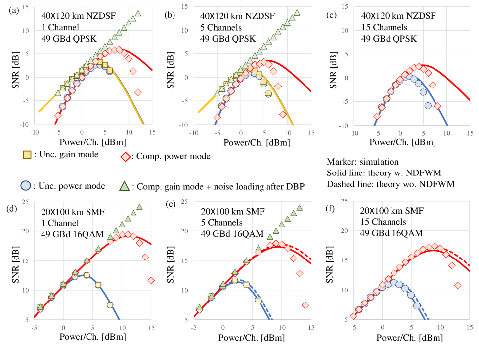
Figure 1: Comparison between numerical simulations (markers), and theoretical curves (lines), top row: configuration 1, bottom row configuration. 2. For each configuration, PDM WDM transmission with 1, 5, and 15 channels are considered. Unc.: uncompensated (i.e. no full-field DBP), Comp.: compensated (i.e. full-field DBP applied at receiver side). For 1- and 5-channel scenarios uncompensated transmission is performed both in gain mode and in power mode.

Figure 1 illustrates the numerical and theoretical SNR vs. per channel lunch power for the two configurations, and for 1, 5, and 15 WDM channels. Fig. 1 top row corresponds to configuration 1, and Fig. 1 bottom row corresponds to configuration 2. Fig. 1a shows the SNR curves of single-channel transmission of configuration 1. The blue circles are numerical results corresponding to the uncompensated (Unc.) transmission where all EDFAs operate at constant output power (power mode), and the yellow squares correspond to the uncompensated transmission case where EDFAs deliver constant signal gain to fully compensate the span loss (gain mode). The solid lines are the theoretical SNR vs. channel power curves as per Eqs. (120) and (121). Red diamonds are numerical results when full-field DBP is applied at the receiver side to the waveforms in the power mode. We also applied full-field compensation to the waveforms in the gain mode, but the results are not shown here in order to avoid cluttering the figures. For sanity check we also did numerical simulations with noiseless transmission followed by full-field DBP, and then loaded the noise after the DBP. This case was simulated to make sure that in absence of noise the nonlinear channel is perfectly inverted. The results of this case are shown in green triangles, and confirm that in the absence of in-line noise, the full-field zero-forcing DBP nonlinear compensation is perfect. In configuration 1 signal depletion by ASE is not negligible, and that is why the uncompensated curves assuming gain mode and power mode are different specially in the linear regime. Both of these uncompensated numerical curves match very well with the corresponding theoretical curves. As to the compensated case, we observe that the theoretical (solid red) curve, Eq. (121), matches the numerical results (red diamonds) up to the optimum power, but then there is a discrepancy between the theoretical and the numerical curves. The same behavior is observed (but not shown in Fig. 1) when compensation is applied to waveforms transmitted the gain mode. The explanation of this divergence is the following: if the nonlinear channel is perfectly inverted, signal-signal interactions are canceled to all orders. We have verified that this is so in noiseless transmission followed by full-field DBP (green triangles), which corresponds to when the compensated SNR would be $SNR_{C}(P)=\sigma^{-2}_{ASE,DP}$ instead of (121); however, if in-line noise is present, the power profile applied in the backpropagation is not exactly the inverted version of the power profile of the forward propagation part, and this asymmetry in the forward and backward portions of signal propagation results in the presence of the residual signal-signal nonlinear distortions, whereas the theoretical curve based on (121) assumes signal-signal nonlinear distortions are perfectly compensated to all orders. Interestingly, our theory well approximates the compensated performance up to the optimum point, and is sufficient to evaluate the fundamental zero-forcing limit of full-field DBP. Figs. 1b and 1c illustrate numerical and theoretical SNR vs. power curves assuming configuration 1, but with 5 and 15 WDM transmitted channels. Figs. 1b and 1c show the SNRs of the third among five, and eight among fifteen channels respectively. similar trends are observed in Figs. 1a, 1b, and 1c. We have thus verified that our theory successfully predicts the performance of the uncompensated transmission in a case where signal depletion by in-line ASE is significant. We also verified that our theory is sufficient to predict system performance assuming full-field DBP up to the optimum power. Figs. 1d, 1e, and 1f illustrate numerical and theoretical SNR vs. power curves in configuration 2. In this scenario signal depletion by ASE is negligible, and uncompensated performance in gain mode and power mode are essentially the same. For configuration 2, we plotted the theoretical curves, both with NDFWM contributions included, solid lines, and with NDFWM terms excluded, dashed lines, in order to assess the importance of NDFWM. the NDFWM terms do not exist in single-channel transmission, Fig. 1d. We observed in Fig. 1e and 1f that excluding NDFWM results in over-estimating the SNR by 0.5 dB and 0.7 dB respectively. We also observe that the red solid curves corresponding to the complete theory with NDFWM included slightly underestimate the numerical curves although the underestimation is about 0.5 dB. This might be partly due to the statistical uncertainty of the estimate numerical SNR, and the limited accuracy of the numerical simulator, and partly due to the inherent approximations in our theory. This issue will be explored further in future research.

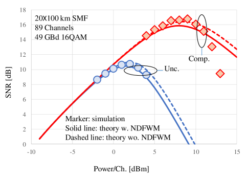
Figure 2: SNR vs. power of the central channel in 89-channel transmission simulation of configuration 2.

Fig.2 illustrates numerical and theoretical SNR vs. power curves in configuration 2, but when 89 WDM channels are transmitted. The COI is the central, i.e., the forty fifth channel. The massive WDM simulations in the compensated case took two weeks to finish using an NVIDIA Tesla K40 GPU card.

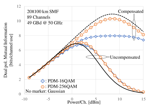
Figure 3: Dual polarization mutual information of 16QAM, 256QAM and Gaussian constellations in configuration two, with and without full-field digital-back propagation post-compensation.

Fig.3 illustrates the mutual information (MI) vs. channel power in configuration 2 with and without full-field nonlinear compensation. We examined 16QAM, 256QAM and constellation, and for the reference, also computed the MI of a Gaussian source. In the uncompensated case the optimum MI of the Gaussian source is less than that of 16QAM and 256 QAM, due to its higher fourth and sixth moments. In the fully-compensated case 16QAM optimum MI saturates to its dual polarization maximum constrained capacity, i.e., 8 bits/channel use, 256QAM optimum MI is 10.3 bits/channel use, and Gaussian source optimum MI is 10.9 bits/channel use.

V Conclusions

In this work we presented a rigorous derivation of a general theory of nonlinear signal-noise interactions in WDM fiber-optic coherent transmission systems. This theory is based on the regular perturbation approximation of the nonlinear Schrödinger equation, and is exact up to the first-order. The theory is general in that, it is valid for dispersion-managed/un-managed systems, all cross-channel nonlinear FWM terms, and the impact of modulation format are taken into account. Heterogeneous spans with both erbium-doped fiber and Raman amplification are allowed, and chromatic dispersion to all-orders can be included. This theory was applied to compute the total variance of the signal distortions at the receiver. Ideal multi-channel digital backpropagation was optionally included in the receiver side. The variance of the signal distortion was expressed as a sum of various signal-signal and signal-noise contributions. First, integral representations were derived for these contributions, and then these representations were further manipulated to obtain equivalent forms, which could be efficiently computed by Standard Monte Carlo integration. The validity of the developed theory was examined by comparing the theoretical signal-to-noise ratio vs. launched power curves with the corresponding numerical curves from WDM transmission simulations using split-step Fourier method. Two link configurations and four channel counts, (1, 5, 15, and 89) were examined. In all the scenarios the theory could predict the optimum uncompensated and compensated performance up to 0.5 dB of discrepancy.

In this appendix the $\mathcal{X}$-coefficients appearing in the formula for the variance of nonlinear signal-signals distortions in (101), and the $\chi$-coefficients appearing in the formula for the variance of NSNI in (113) are computed. In -A we derive integral representations for $\mathcal{X}$ and $\chi$-coefficients. In -B we simplify these integral representations. In -C, the simplified integral representations are further manipulated to do efficient numerical computations.

-A Integral representation of $\mathcal{X}$- and $\chi$-coefficients

Consider the following spectral-domain integral representation of the kernel integrals in (100)

$$K_{m,n,p}^{\left({s,s^{\prime}}\right)}\left(z\right)=\int_{{\rm I\!R}^{3}}{\frac{{{d^{3}}\omega}}{{{{\left({2\pi}\right)}^{3}}}}}{H_{{\vec{\omega}},s,s^{\prime}}}\left(z\right){e^{i\left({m{\omega_{1}}-p{\omega_{2}}+n{\omega_{3}}}\right)T}}.$$ (122)

Throughout this work the symbol $d^{n}\omega$ stands for $d\omega_{1}d\omega_{2}\cdots d\omega_{n}$ for any positive integer $n$, and the following notational convention is used

$$\vec{\omega}=\left({{\omega_{1}},{\omega_{2}},{\omega_{3}}}\right).$$ (123)

The integrand function in (122) is

$$H_{\vec{\omega},s,s^{\prime}}(z)=\Pi_{\vec{\omega},s,s^{\prime}}f(z)e^{i\beta_{2}(z)(\omega_{2}-\omega_{3})(\omega_{2}-\omega_{1})},$$ (124)

where, the function $\Pi_{\vec{\omega},s,s^{\prime}}$ is defined to be

$$\Pi_{\vec{\omega},s,s^{\prime}}=\tilde{u}_{0}^{(0)}(0,\omega_{1}-\Omega_{s})\tilde{u}{{}_{0}^{(0)*}}(0,\omega_{2}-\Omega_{s+s^{\prime}})\times\\ \tilde{u}_{0}^{(0)}(0,\omega_{3}-\Omega_{s^{\prime}})\tilde{u}{{}_{0}^{(0)*}}\left({0,{\omega_{1}}-{\omega_{2}}+{\omega_{3}}}\right).$$ (125)

Note that the following notional simplifications are used in the following: $H_{\vec{\omega},s}=H_{\vec{\omega},0,s}$, $\Pi_{\vec{\omega},s}=\Pi_{\vec{\omega},0,s}$, $H_{\vec{\omega}}=H_{\vec{\omega},0,0}$, and $\Pi_{\vec{\omega}}=\Pi_{\vec{\omega},0,0}$. For the $\mathcal{X}$-coefficients contributing to the variance of nonlinear signal-signal distortions, the following expressions are derived, [19, 20, 21, 22],

$$\mathcal{X}_{1}=\sum\limits_{m,n,p}{{{\left|{X_{m,n,p}^{\left({0,0}\right)}}\right|}^{2}}},$$ (126)

$$\mathcal{X}_{2}=\sum\limits_{m,n}{{{\left|{X_{m,m,n}^{\left({0,0}\right)}}\right|}^{2}}},$$ (127)

$$\mathcal{X}_{3}=\sum\limits_{m,n}{{{\left|{X_{m,n,n}^{\left({0,0}\right)}}\right|}^{2}}},$$ (128)

$$\mathcal{X}_{4}=\operatorname{Re}\left\{{\sum\limits_{m,n}{X_{m,n,n}^{\left({0,0}\right)}X{{{}_{m,m,m}^{\left({0,0}\right)}}^{*}}}}\right\},$$ (129)

$$\mathcal{X}_{5}=\sum\limits_{m}{{{\left|{X_{m,m,m}^{\left({0,0}\right)}}\right|}^{2}}},$$ (130)

$$\mathcal{X}_{1,s}=\sum\limits_{m,n,p}{{{\left|{X_{m,n,p}^{\left({0,s}\right)}}\right|}^{2}}},$$ (131)

$$\mathcal{X}_{3,s}=\sum\limits_{m,n}{{{\left|{X_{m,n,n}^{\left({0,s}\right)}}\right|}^{2}}},$$ (132)

$$\mathcal{X}_{1,s,s^{\prime}}=\sum\limits_{m,n,p}{{{\left|{X_{m,n,p}^{\left({s,s^{\prime}}\right)}}\right|}^{2}}}.$$ (133)

We can replace (122) into (126) to obtain an integral representation for $\mathcal{X}_{1}$, which is written as follows

$$\mathcal{X}_{1}=T^{2}\int_{0}^{L}{dz}\int_{0}^{L}{dz^{\prime}}\sum\limits_{m,n,p}{K_{m,n,p}^{\left({0,0}\right)}\left(z\right)K{{{}_{m,n,p}^{\left({0,0}\right)}}^{*}}\left({z^{\prime}}\right)}.$$ (134)

Similar expressions can be obtained for all other $\mathcal{X}$-coefficients.

In order to simplify the $\chi$-coefficients contributing to the variance of nonlinear signal-noise distortions, we start from (104) and (113), and Eqns. (105)-(112). The following simplified integral representations are resulted

$${\chi_{0}}=T^{2}\int_{0}^{L}{dz}\int_{0}^{L}{dz^{\prime}}\xi(\min(z,z^{\prime});0)\times\\ \sum\limits_{m,n,p}{}K_{m,n,n}^{\left({0,0}\right)}\left(z\right)K_{m,p,p}^{(0,0)*}\left({z^{\prime}}\right),$$ (135)

$${\chi_{1}}=T^{2}\int_{0}^{L}{dz}\int_{0}^{L}{dz^{\prime}}\xi(\min(z,z^{\prime});0)\times\\ \sum\limits_{m,n,p}K_{m,n,p}^{(0,0)}(z)K{{}_{m,n,p}^{(0,0)*}}(z^{\prime}),$$ (136)

$${\chi_{2}}=T^{2}\int_{0}^{L}{dz}\int_{0}^{L}{dz^{\prime}}\xi(\min(z,z^{\prime});0)\times\\ \sum\limits_{m,n}{}K_{m,m,n}^{\left({0,0}\right)}\left(z\right)K{{}_{m,m,n}^{(0,0)*}}\left({z^{\prime}}\right),$$ (137)

$${\chi_{3}}=T^{2}\int_{0}^{L}{dz}\int_{0}^{L}{dz^{\prime}}\xi(\min(z,z^{\prime});0)\times\\ \sum\limits_{m,n}{}K_{m,n,n}^{\left({0,0}\right)}\left(z\right)K{{}_{m,n,n}^{(0,0)*}}\left({z^{\prime}}\right),$$ (138)

$${\chi_{0,s}}=T^{2}\int_{0}^{L}{dz}\int_{0}^{L}{dz^{\prime}}\xi(\min(z,z^{\prime});0)\times\\ \sum\limits_{m,n,p}{}K_{m,n,n}^{\left({0,s}\right)}\left(z\right)K{{}_{m,p,p}^{(0,s)*}}\left({z^{\prime}}\right),$$ (139)

$${\chi_{1,s}}=T^{2}\int_{0}^{L}{dz}\int_{0}^{L}{dz^{\prime}}\xi(\min(z,z^{\prime});0)\times\\ \sum\limits_{m,n,p}{}K_{m,n,p}^{\left({0,s}\right)}\left(z\right)K{{}_{m,n,p}^{(0,s)*}}\left({z^{\prime}}\right),$$ (140)

$${\chi^{\prime}_{1,s}}=T^{2}\int_{0}^{L}{dz}\int_{0}^{L}{dz^{\prime}}\xi(\min(z,z^{\prime});\Omega_{s})\times\\ \sum\limits_{m,n,p}{}K_{m,n,p}^{\left({0,s}\right)}\left(z\right)K{{}_{m,n,p}^{(0,s)*}}\left({z^{\prime}}\right)$$ (141)

$${\chi_{3,s}}=T^{2}\int_{0}^{L}{dz}\int_{0}^{L}{dz^{\prime}}\xi(\min(z,z^{\prime});0)\times\\ \sum\limits_{m,n}{}K_{m,n,n}^{\left({0,s}\right)}\left(z\right)K{{}_{m,n,n}^{(0,s)*}}\left({z^{\prime}}\right),$$ (142)

-B Simplifying integral representations

The goal of this subsection is to simplify the integral representation of the $\mathcal{X}$- and $\chi$-coefficients derived in the previous subsection, i.e., Eqs. (134)-(142), by carrying out the discrete sums over symbol indices. Following the idea introduced in[19, 20, 21, 22] let’s consider the the following identity

$$\sum\limits_{m=-\infty}^{+\infty}{{e^{im\omega T}}}=\frac{{2\pi}}{T}\sum\limits_{m=-\infty}^{+\infty}{\delta\left({\omega-\frac{{2\pi m}}{T}}\right)},$$ (143)

as well as the following orthogonality condition, which holds for Nyquist pulses

$$\tilde{u}_{0}^{\left(0\right)}\left({0,\omega}\right)\tilde{u}{{}_{0}^{(0)*}}\left({0,\omega-\frac{{2\pi n}}{T}}\right)={\left|{\tilde{u}_{0}^{\left(0\right)}\left({0,\omega}\right)}\right|^{2}}{\delta_{0n}}.$$ (144)

Using these two basic relations, the discrete summations can be carried out in Eqs. (134)-(142). The following simplified integral representations are found for the $\mathcal{X}$-coefficients appearing in the variance of the signal-signal distortions, (101),

$$\mathcal{X}_{1}=\frac{1}{T}\int_{{\rm I\!R}^{4}}{\frac{{{d^{3}}\omega}}{{{{\left({2\pi}\right)}^{3}}}}\int_{0}^{L}{dz{H_{\vec{\omega}}}\left(z\right)}}\int_{0}^{L}{dz^{\prime}}H_{\vec{\omega}}^{*}\left({z^{\prime}}\right),$$ (145)

$$\mathcal{X}_{2}=\int_{{\rm I\!R}^{4}}{\frac{{{d^{4}}\omega}}{{{{\left({2\pi}\right)}^{4}}}}\int_{0}^{L}{dz{H_{\vec{\omega}}}\left(z\right)\int_{0}^{L}{dz^{\prime}}H_{\vec{\omega}^{\prime}}^{*}\left({z^{\prime}}\right)}},$$ (146)

$$\mathcal{X}_{3}=\int_{{\rm I\!R}^{4}}{\frac{{{d^{4}}\omega}}{{{{\left({2\pi}\right)}^{4}}}}\int_{0}^{L}{dz{H_{\vec{\omega}}}\left(z\right)\int_{0}^{L}{dz^{\prime}}H_{\vec{\omega}^{\prime\prime}}^{*}\left({z^{\prime}}\right)}},$$ (147)

$$\mathcal{X}_{4}=\int_{{\rm I\!R}^{3}}{\frac{{{d^{3}}\omega}}{{{{\left({2\pi}\right)}^{3}}}}\int_{0}^{L}{dzH_{\vec{\omega}^{\prime\prime}}^{*}\left(z\right)}},$$ (148)

$$\mathcal{X}_{5}=T\int_{{\rm I\!R}^{4}}{\frac{{{d^{5}}\omega}}{{{{\left({2\pi}\right)}^{5}}}}\int_{0}^{L}{dz{H_{\vec{\omega}}}\left(z\right)\int_{0}^{L}{dz^{\prime}}H_{\vec{\omega}^{\prime\prime\prime}}^{*}\left({z^{\prime}}\right)}},$$ (149)

$$\mathcal{X}_{1,s}=\frac{1}{T}\int{\frac{{{d^{3}}\omega}}{{{{\left({2\pi}\right)}^{3}}}}\int_{0}^{L}{dz{H_{\vec{\omega},s}}\left(z\right)}}\int_{0}^{L}{dz^{\prime}}H_{\vec{\omega},s}^{*}\left({z^{\prime}}\right),$$ (150)

$$\mathcal{X}_{3,s}=\int{\frac{{{d^{4}}\omega}}{{{{\left({2\pi}\right)}^{4}}}}\int_{0}^{L}{dz{H_{\vec{\omega},s}}\left(z\right)\int_{0}^{L}{dz^{\prime}}H_{\vec{\omega}^{\prime\prime},s}^{*}\left({z^{\prime}}\right)}},$$ (151)

$$\mathcal{X}_{1,s,s^{\prime}}=\frac{1}{T}\int{\frac{{{d^{3}}\omega}}{{{{\left({2\pi}\right)}^{3}}}}\int_{0}^{L}{dz{H_{\vec{\omega},s,s^{\prime}}}\left(z\right)}}\int_{0}^{L}{dz^{\prime}}H_{\vec{\omega},s,s^{\prime}}^{*}\left({z^{\prime}}\right).$$ (152)

The following integral representations are found for the $\chi$-coefficients appearing in in the variance of NSNI distortions, (113),

$${\chi_{0}}=2\int_{0}^{L}{dzf(z)}\int_{0}^{z}{dz^{\prime}}f(z^{\prime})\xi(z^{\prime};0),$$ (153)

$${\chi_{1}}=\frac{2}{{T}}{\mathop{\rm Re}\nolimits}\left\{\int_{{\rm I\!R}^{3}}\frac{d^{3}\omega}{{(2\pi)}^{3}}\times\right.\\ \left.{\int_{0}^{L}{dz{H_{\vec{\omega}}}\left(z\right)}\int_{0}^{z}{dz^{\prime}H_{\vec{\omega}}^{*}\left({z^{\prime}}\right)}\xi(z^{\prime};0)}\right\},$$ (154)

$${\chi_{2}}=2{\mathop{\rm Re}\nolimits}\left\{\int_{{\rm I\!R}^{4}}\frac{d^{4}\omega}{{(2\pi)}^{4}}\times\right.\\ \left.{\int_{0}^{L}{dz{H_{\vec{\omega}}}\left(z\right)}\int_{0}^{z}{dz^{\prime}H_{\vec{\omega}^{\prime}}^{*}\left({z^{\prime}}\right)}\xi(z^{\prime};0)}\right\},$$ (155)

$${\chi_{3}}=2{\mathop{\rm Re}\nolimits}\left\{\int_{{\rm I\!R}^{4}}\frac{d^{4}\omega}{{(2\pi)}^{4}}\times\right.\\ \left.{\int_{0}^{L}{dz{H_{\vec{\omega}}}\left(z\right)}\int_{0}^{z}{dz^{\prime}H_{\vec{\omega}^{\prime\prime}}^{*}\left({z^{\prime}}\right)}\xi(z^{\prime};0)}\right\},$$ (156)

$${\chi_{1,s}}={\frac{2}{{{T}}}}{\mathop{\rm Re}\nolimits}\left\{\int_{{\rm I\!R}^{3}}\frac{d^{3}\omega}{{(2\pi)}^{3}}\times\right.\\ \left.{\int_{0}^{L}{dz{H_{\vec{\omega},s}}\left(z\right)}\int_{0}^{z}{dz^{\prime}H_{\vec{\omega},s}^{*}\left({z^{\prime}}\right)}\xi(z^{\prime};0)}\right\},$$ (157)

$${{\chi^{\prime}}_{1,s}}={\frac{2}{{{T}}}}{\mathop{\rm Re}\nolimits}\left\{\int_{{\rm I\!R}^{3}}\frac{d^{3}\omega}{{(2\pi)}^{3}}\times\right.\\ \left.{\int_{0}^{L}{dz{H_{\vec{\omega},s}}\left(z\right)}\int_{0}^{z}{dz^{\prime}H_{\vec{\omega},s}^{*}\left({z^{\prime}}\right)}\xi(z^{\prime};\Omega_{s})}\right\},$$ (158)

$${\chi_{3,s}}=2{\mathop{\rm Re}\nolimits}\left\{\int_{{\rm I\!R}^{4}}\frac{d^{4}\omega}{{(2\pi)}^{4}}\times\right.\\ \left.{\int_{0}^{L}{dz{H_{\vec{\omega},s}}\left(z\right)}\int_{0}^{z}{dz^{\prime}H_{\vec{\omega}^{\prime\prime},s}^{*}\left({z^{\prime}}\right)}\xi(z^{\prime};0)}\right\},$$ (159)

where, we have used the shorthand notations

$$\vec{\omega}^{\prime}=\left({{\omega_{4}},{\omega_{2}},{\omega_{1}}+{\omega_{3}}-{\omega_{4}}}\right),$$ (160)

and

$$\vec{\omega}^{\prime\prime}=\left({{\omega_{1}},{\omega_{4}},{\omega_{3}}-{\omega_{2}}+{\omega_{4}}}\right).$$ (161)

Note that $\chi_{0,s}=\chi_{0}$. The coefficients $\chi_{0}$ and $\chi_{0,s}$ model the average phase rotation due to nonlinear-signal-noise interactions and will not contribute to the variance of the nonlinear distortions.

-C Efficient integration

The integral representations derived in the previous subsection for $\mathcal{X}$-coefficients, Eqns. (145)-(152), and for $\chi$-coefficients, Eqns. (153)-(159), have to be evaluated numerically; however, numerical integration of those equations can be still time consuming. In this subsection, we assume EDFA-only optical amplification, and carry out the $z$-integrals. The remaining multidimensional $\omega$ integrals can be efficiently computed by standard Monte Carlo integration. We present the detailed computation only for $\chi_{2}$ and $\mathcal{X}_{2}$ to save space. The same procedure can be applied to all other $\mathcal{X}$ and $\chi$-coefficients.

Let’s consider the integral representation of $\chi_{2}$ as per (155), which is rewritten in a slightly different form as

$$\chi_{2}=2\mathop{\rm Re}\nolimits\{\int_{{\rm I\!R}^{4}}\frac{d^{4}\omega}{{(2\pi)}^{4}}{R_{\vec{\omega},\vec{\omega}^{\prime}}}\},$$ (162)

where, the integrand function $R_{\vec{\omega},\vec{\omega}^{\prime}}$ is

$${R_{\vec{\omega},\vec{\omega}^{\prime}}}=\int_{0}^{L}{dz}{H_{\vec{\omega}}}\left(z\right){h_{\vec{\omega}^{\prime}}}\left(z\right),$$ (163)

The function $h_{\vec{\omega}^{\prime}}(z)$ in (163) is

$${h_{\vec{\omega}^{\prime}}}\left(z\right)=\int_{0}^{z}{dz^{\prime}}H_{\vec{\omega}^{\prime}}^{*}\left({z^{\prime}}\right)\xi\left({z^{\prime};0}\right).$$ (164)

We also define the set of auxiliary variables $\{\psi_{n}\}$, for $n=1,\cdots,N_{s}$ as

$${\psi_{n}}=\sum\limits_{j=0}^{n-1}{{\xi_{j}(0)}}.$$ (165)

Now we substitute (68) into (164), and use (165). After doing some algebra we obtain

$${h_{\vec{\omega}^{\prime}}}\left(z\right)={h_{\vec{\omega}^{\prime},m}}+{\psi_{m}}\int_{{z_{m-1}}}^{z}{dz^{\prime}}H_{\vec{\omega}^{\prime}}^{*}\left({z^{\prime}}\right)\\ {z_{m-1}}\leq z<{z_{m}},m=1,\ldots,{N_{s}},$$ (166)

where,

$${h_{\vec{\omega}^{\prime},m}}=\sum\limits_{j=0}^{m-1}{{\psi_{j}}r_{\vec{\omega}^{\prime},j}^{*}},$$ (167)

and

$${r_{\vec{\omega},m}}=\int_{{z_{m-1}}}^{{z_{m}}}{dz^{\prime}{H_{\vec{\omega}}}\left({z^{\prime}}\right)}.$$ (168)

If we assume that $\beta_{2}(z)={\beta_{2,m}}$, and $\alpha(z)={\alpha_{m}}$ for $z_{m-1}\leq z<{z_{m}}$, The integration in (168) can be carried out to obtain

$$r_{\vec{\omega},m}=e^{-\delta_{m-1}}\frac{{{e^{i{\varphi_{\vec{\omega},m}}{z_{m-1}}}}-{\eta_{m}}{e^{i{\varphi_{\vec{\omega},m}}{z_{m}}}}}}{{{\alpha_{m}}-i{\varphi_{\vec{\omega},m}}}}{\Pi_{\vec{\omega}}},$$ (169)

where, the phase factor due to dispersion is

$$\varphi_{\vec{\omega},m}={\beta_{2,m}}\left({{\omega_{2}}-{\omega_{1}}}\right)\left({{\omega_{2}}-{\omega_{3}}}\right).$$ (170)

The field span loss is

$$\eta_{m}={e^{-{\alpha_{m}}({{z_{m}}-{z_{m-1}}})}}.$$ (171)

Now we rewrite (163) as a sum over spans as follows

$$R_{\vec{\omega},\vec{\omega}^{\prime}}=\sum\limits_{m=1}^{{N_{s}}}{\int_{{z_{m-1}}}^{{z_{m}}}{dz}{H_{\vec{\omega}}}\left(z\right){h_{\vec{\omega}^{\prime}}}\left(z\right)},$$ (172)

and substitute (166) into (172). The following formula is derived for $R_{\vec{\omega},\vec{\omega}^{\prime}}$

$${R_{\vec{\omega},\vec{\omega}^{\prime}}}=\sum\limits_{m=1}^{{N_{s}}}{{r_{\vec{\omega},m}}}{h_{\vec{\omega}^{\prime},m}}+\sum\limits_{m=1}^{{N_{s}}}{{\psi_{m}}}{I_{\vec{\omega},\vec{\omega}^{\prime},m}},$$ (173)

where,

$$I_{\vec{\omega},\vec{\omega}^{\prime},m}=\int_{{z_{m-1}}}^{{z_{m}}}{dz}{H_{\vec{\omega}}}\left(z\right)\int_{{z_{m-1}}}^{z}{dz^{\prime}}H_{\vec{\omega}^{\prime}}^{*}(z^{\prime}).$$ (174)

The integral in the right hand side of (174) is calculated in a straightforward manner, to obtain

$${I_{\vec{\omega},\vec{\omega}^{\prime},m}}={\Pi_{\vec{\omega}}}{\Pi_{\vec{\omega}^{\prime}}}\frac{{{e^{-2{\delta_{m-1}}+i\left({{\varphi_{\vec{\omega},m}}-{\varphi_{\vec{\omega}^{\prime},m}}}\right){z_{m-1}}}}}}{{{\alpha_{m}}+i{\varphi_{\vec{\omega}^{\prime},m}}}}\times\\ \{\frac{{1-{\eta_{m}}{e^{i{\varphi_{\vec{\omega},m}}\left({{z_{m}}-{z_{m-1}}}\right)}}}}{{{\alpha_{m}}-i{\varphi_{\vec{\omega},m}}}}-\\ \frac{{1-\eta_{m}^{2}{e^{i(\varphi_{\vec{\omega},m}-\varphi_{\vec{\omega}^{\prime},m})(z_{m}-z_{m-1})}}}}{{2{\alpha_{m}}-({\varphi_{\vec{\omega},m}}-\varphi_{\vec{\omega}^{\prime},m})}}\}.$$ (175)

Putting it all together, the coefficient $\chi_{2}$ can be evaluated by the following four-dimensional integral

$$\chi_{2}=\\ 2\operatorname{Re}\left\{{\int_{V}{\frac{{{d^{4}}\omega}}{{{{\left({2\pi}\right)}^{4}}}}}}\right.\left.{\left[{\sum\limits_{m=1}^{{N_{s}}}{{r_{\vec{\omega},m}}}{h_{\vec{\omega}^{\prime},m}}+\sum\limits_{m=1}^{{N_{s}}}{{\psi_{m}}}{I_{\vec{\omega},\vec{\omega}^{\prime},m}}}\right]}\right\},$$ (176)

where, $V=\left\{{\left({{\omega_{1}},{\omega_{2}},{\omega_{3}},{\omega_{4}}}\right)\in{{\rm I\!R}^{4}}\left|{{\Pi_{\vec{\omega}}}{\Pi_{\vec{\omega}^{\prime}}}\neq 0}\right.}\right\}$ is a four-dimensional subset of the four-dimensional real space. The integral in (176) can be efficiently computed by Monte Carlo sampling of the four-dimensional region $V$.

A similar procedure can be applied to efficiently compute all other $\chi$-coefficients. In order to compute $\chi_{3}$ and $\chi_{3,s}$, we have to replace $\vec{\omega}^{\prime}$ with $\vec{\omega}^{\prime\prime}$ in (176). To compute $\chi_{3,s}$, we also have to replace $H_{\vec{\omega}}$ in (168) with $H_{\vec{\omega},s}$. In order to compute $\chi_{1}$, $\chi_{1,s}$ and $\chi^{\prime}_{1,s}$ we have to replace $\vec{\omega}^{\prime}$ with $\vec{\omega}$ in (163)-(176). In this case the right hnd side of (175) is considerbaly simplified, and we obtain

$$\operatorname{Re}\left\{{{I_{\vec{\omega},\vec{\omega},m}}}\right\}=\frac{1}{2}{\left|{{r_{\vec{\omega},m}}}\right|^{2}}.$$ (177)

For computing $\chi^{\prime}_{1,s}$ we also have to replace $\xi_{j}(0)$ with $\xi_{j}(\Omega_{s})$ in (165).

The same approach can be applied, with much less pain, to efficiently integrate $\mathcal{X}$-coefficients. For instance, the following expression is derived for $\mathcal{X}_{2}$

$$\mathcal{X}_{2}=\int_{{\rm I\!R}^{4}}{\frac{{{d^{4}}\omega}}{{{{\left({2\pi}\right)}^{4}}}}}\left({\sum\limits_{m=1}^{{N_{s}}}{{r_{\vec{\omega},m}}}}\right)\left({\sum\limits_{m=1}^{{N_{s}}}{r_{\vec{\omega}^{\prime},m}^{*}}}\right).$$ (178)

References

• [1] G. P. Agrawal, “Nonlinear Fiber Optics”, Academic Press, 2007.
• [2] R. -J. Essiambre, G. Kramer, P. J. Winzer, G. J. Foschini, B. Goebel, “Capacity Limits of Optical Fiber Networks”,IEEE J. Lightwave.Technol., vol. 28, no. 4, Feb., 2010.
• [3] A. Ghazisaeidi, L. Schmalen, I. Fernandez de Jauregui, P. Tran, C. Simonneau, P. Brindel, and G. Charlet, “52.9 Tb/s Transmission over Transoceanic Distances using Adaptive Multi-Rate FEC”,in Proc. ECOC, Paper PD.3.4, Cannes, France, 2014.
• [4] A. Ghazisaeidi, L. Schmalen, I. Fernandez de Jauregui Ruiz, P. Tran, C. Simonneau, P. Brindel, and G. Charlet, “Transoceanic Transmission Systems Using Adaptive Multirate FECs”, IEEE J. Lightw. Technol., vol. 33, no.7, pp. 1479-1487, Apr. 2015.
• [5] A. Ghazisaeidi, L. Schmalen, P. Tran, C. Simonneau, E. Awwad, B. Uscumlic, P. Brindel, and G. Charlet, “54.2 Tb/s transoceanic transmission using ultra low loss fiber, multi-rate FEC and digital nonlinear mitigation” , in Proc. ECOC, Paper Th.2.2.3, Valencia, Spain, 2015.
• [6] A. Ghazisaeidi, I. Fernandez de Jauregui Ruiz, L. Schmalen, P. Tran, C. Simonneau, E. Awwad, B. Uscumlic, P. Brindel, and G. Charlet., “Submarine Transmission Systems Using Digital Nonlinear Compensation and Adaptive Rate Forward Error Correction”,IEEE, J. Lightwave Technol., Vol. 34, no. 8, p. 188 (2016).
• [7] A. Ghazisaeidi, I. Fernandez de Jauregui Ruiz, R. Rios-Müller, L. Schmalen, P. Tran, P. Brindel, A. Carbo Meseguer, Q. Hua, F. Buchali, G. Charlet, and J. Renaudier, “65Tb/s Transoceanic Transmission Using Probabilistically-Shaped PDM-64QAM”,in Proc. ECOC, Paper Th.3.C.4, Düsseldorf, Germany, 2016.
• [8] A. Ghazisaeidi, I. Fernandez de Jauregui Ruiz, R. Rios-Müller, L. Schmalen, P. Tran, P. Brindel, A. Carbo Meseguer, Q. Hu, F. Buchali, G. Charlet and J. Renaudier, “Advanced C+L-Band Transoceanic Transmission Systems Based on Probabilistically-Shaped PDM-64QAM”, IEEE, J. Lightwave Technol., early access (2017).
• [9] S. Zhang, F. Yaman, Y. -K. Huang, J. D. Downie, D. Zou, W. A. Wood, A. Zakharian, R. Khrapko, S. Mishra, V. Nazarov, J. Hurley, I. B. Djordjevic, E. Mateo, and Y. Inada., “Capacity-Approaching Transmission over 6375 km at Spectral Efficiency of 8.3 bit/s/Hz”, Proc. OFC, Th5C.2, Anaheim (2016).
• [10] J. -X. Cai, H. G. Batshon, M. V. Mazurczyk, O. V. Sinkin, D. Wang, M. Paskov, W. Patterson, C. R. Davidson, P. Corbett, G. Wolter, T. Hammon, M. Bolshtyansky, D. Foursa and A. Pilipetskii, “70.4 Tb/s Capacity over 7,600 km in C+L Band Using Coded Modulation with Hybrid Constellation Shaping and Nonlinearity Compensation”, Proc. OFC, Th5B.2, Los Angeles (2017).
• [11] F. Vacondio, O. Rival, C. Simonneau, E. Grellier, A. Bononi, L. Lorcy, J. -C. Antona, and S. Bigo, “On nonlinear distortions of highly dispersive optical coherent systems”, Opt. Express 20, 1022-1032 (2012).
• [12] X. Chen and W. Shieh, “Closed-form expressions for nonlinear transmission performance of densely spaced coherent optical OFDM systems”’, Opt. Exp., vol. 18, pp. 19039–19054, Aug. 2010.
• [13] P. Poggiolini, A. Carena, V. Curri, G. Bosco, and F. Forghieri, “Analytical Modeling of Nonlinear Propagation in Uncompensated Optical Transmission Links”,IEEE Photon. Technol. Lett., vol. 23, no. 11, pp. 742-744, June 2011.
• [14] A. Carena, V. Curri, G. Bosco, P. Poggiolini, and F. Forghieri, “Modeling of the Impact of Nonlinear Propagation Effects in Uncompensated Optical Coherent Transmission Links”, IEEE J. Lightwave Technol. Vol. 30, no. 10, pp. 1524-1539, May 2012.
• [15] P. Poggiolini, G. Bosco, A. Carena, V. Curri, Y. Jiang, and F. Forghieri, “The GN-Model of Fiber Non-Linear Propagation and its Applications”, IEEE J. Lightwave Technol. Vol. 32, no. 4, pp. 694-721, February 2014.
• [16] P. Johannisson and M. Karlsson, “Perturbation Analysis of Nonlinear Propagation in a Strongly Dispersive Optical Communication Systems”, IEEE J. Lightwave Technol. Vol. 31, no. 8, pp. 1273-1282, April 2013.
• [17] A. Mecozzi and R. -J. Essiambre, “Nonlinear Shannon Limit in Pseudolinear Coherent Limit”,J. Lightwave Technol. vol. 30, no. 12, pp. 2011-2014 (2012).
• [18] A. Mecozzi, C. B. Clausen, and M. Shtaif, “System impact of intra-channel nonlinear effects in highly dispersed optical pulse transmission”, IEEE Photon. Technol. Lett. . Vol. 12, no. 12, pp. 1633-1635, December 2000.
• [19] R. Dar, M. Feder, A. Mecozzi, and M Shtaif, “Properties of nonlinear noise in long dispersion-uncompensated fiber links”, Optics Express, vol. 21, no. 22, pp. 25685-25699, October 2013.
• [20] R. Dar, M. Feder, A. Mecozzi, and M Shtaif, “Accumulation of nonlinear interference noise in fiber-optic systems”, Optics. Express, vol. 22, no. 12 pp.14199-14211, May. 2014.
• [21] R. Dar, M. Feder, A. Mecozzi, and M Shtaif, “Inter-Channel Nonlinear Interference Noise in WDM Systems: Modeling and Mitigation”, IEEE J. Lightwave Technol., vol. 33, no. 5, pp. 1044-1053, March 2015.
• [22] R. Dar, M. Feder, A. Mecozzi, and M Shtaif, “Pulse Collision Picture of Inter-Channel Nonlinear Interference in Fiber-Optic Communications”, IEEE J. Lightwave Technol., vol. 34, no. 2, pp. 593-607, January 2016.
• [23] A. Carena, G. Bosco, V. Curri, Y. Jiang, P. Poggiolini, and F. Forghieri, “EGN model of non-linear fiber propagation”, Optics. Express, vol. 22, no. 13 pp.16335-16362, May. 2014.
• [24] O. Golani, R. Dar, M. Feder, A. Mecozzi, and M. Shtaif, “Modeling the Bit-Error-Rate Performance of Nonlinear Fiber-Optic Systems”, J. Lightwave Technol. 34, 3482-3489 (2016).
• [25] A. Vannucci, P. Serena, and A. Bononi, “The RP method: A new tool for the iterative solution of the nonlinear Schroedinger equation”, J. Lightw. Technol., vol. 20, no. 7, pp. 1102–1112, Jul. 2002.
• [26] P. Serena and A. Bononi, “An Alternative Approach to the Gaussian Noise Model and its System Implications”, IEEE J. Lightwave Technol. Vol. 31, no. 22, pp. 3489-3499, November 2013.
• [27] P. Serena and A. Bononi, “A Time-Domain Extended Gaussian Noise Model”, IEEE J. Lightwave Technol. Vol. 33, no. 7, pp. 1459-1472, April 2015.
• [28] E. Ip and J. Kahn, “Compensation of Dispersion and Nonlinear Impairments Using Digital Backpropagation”, J. Lightwave. Technol., vol. 26, n° 20 pp3416-3425 (2008).
• [29] I. Fernandez de Jauregui Ruiz, A. Ghazisaeidi, and G. Charlet, “Optimization Rules and Performance Analysis of Filtered Digital Backpropagation ”, in Proc. ECOC, Paper , Valencia, Spain, 2015.
• [30] Z. Tao, L. Dou, W. Yan, H. Hoshida, and J. -C. Rasmussen, “Multiplier-Free Intrachannel Nonlinearity Compensating Algorithm Operating at Symbol Rate”, IEEE J. Lightwave Technol. Vol. 29, no. 17, pp. 2570, (2011).
• [31] A. Ghazisaeidi and R. -J. Essiambre, “Calculation of Coefficients of Perturbative Nonlinear Pre-Compensation for Nyquist Pulses”, in Proc. ECOC, Paper We.1.3.3, Cannes, France, 2014.
• [32] R. Dar and P. J. Winzer, “Nonlinear Interference Mitigation: Methods and Potential Gain”, J. Lightwave Technol. (2017).
• [33] D. Rafique and A. D. Ellis, “Impact of signal-ASE four-wave mixing on the effectiveness of digital back-propagation in 112 Gb/s PM-QPSK systems”, Optics. Express, vol. 16, no. 2, pp. 73-85, March. 2011.
• [34] E. Temprana, E. Myslivets, L. Liu, V. Ataie, A. Wiberg, BPP. Kuo, N.. Alic, S. Radic, “Two-fold transmission reach enhancement enabled by transmitter-side digital backpropagation and optical frequency comb-derived information carriers”, Optics. Express, vol. 23, no. 16, pp. 20774-20783, 2015.
• [35] L. Galdino, D. Semrau, D. Lavery, G. Saavedra, C. B. Czegledi, E. Agrell, R. I. Killey, and P. Bayvel, “On the limits of digital back-propagation in the presence of transceiver noise”, Opt. Express 25, 4564-4578 (2017).
• [36] G. Liga, T. Xu, A. Alvarado, R. I. Killey, and P. Bayvel, “On the performance of multichannel digital backpropagation in high-capacity long-haul optical transmission”, Opt. Express 22, 30053-30062 (2014).
• [37] D. Lavery, R. Maher, G. Liga, D. Semrau, L. Galdino, and P. Bayvel, “On the bandwidth dependent performance of split transmitter-receiver optical fiber nonlinearity compensation”, Opt. Express 25, 4554-4563 (2017).
• [38] C. B. Czegledi, G. Liga, D. Lavery, M. Karlsson, E. Agrell, S. J. Savory, and P. Bayvel, “Digital backpropagation accounting for polarization-mode dispersion”, Opt. Express 25, 1903-1915 (2017).
• [39] I. Fernandez de Jauregui Ruiz, A. Ghazisaeidi, E. Awwad, P. Tran, G. Charlet, “Polarization Effects in Nonlinearity Compensated Links”, in Proc. ECOC, Paper , Dusseldorf, Germany, 2016.
• [40] A. D. Ellis, M. A. Z. Al Khateeb, and M. E. McCarthy, “Impact of Optical Phase Conjugation on the Nonlinear Shannon Limit”, in Proc. Optical Fiber Conference, Anaheim, CA, US, 2016, Paper Th4F.2.
• [41] M. I. Yousefi and F. R. Kschischang, “Information Transmission Using the Nonlinear Fourier Transform, Part I: Mathematical Tools”, IEEE Trans Information theory, vol. 60, no. 7, pp. 4312-4328, 2014.
• [42] V. Aref, S. T. Le, and H. Buelow, “Demonstration of Fully Nonlinear Spectrum Modulated System in the Highly Nonlinear Optical Transmission Regime“, in Proc. ECOC, Paper PD.3.4, Dusseldorf, Germany, 2016.
• [43] A. Bononi, P. Serena, and N. Rossi, “Nonlinear signal–noise interactions in dispersion-managed links with various modulation formats”, Optical Fiber Technology, vol. 16, no. 2, pp. 73-85, March 2010.
• [44] D. G. Foursa, O. V. Sinkin, A. Lucero, J. Cai, G. Mohs, and A. Pilipetskii, “Nonlinear interaction between signal and amplified spontaneous emission in coherent systems”, in Proc. Optical Fiber Communication Conf., Anaheim, CA, USA, 2013, Paper JTh2A.35.
• [45] X. Yi, J. Wu, Y. Li, W. Li, X. Hong, H. Guo, Y. Zuo, and J. Lin, “Nonlinear signal-noise interactions in dispersion managed coherent PM-QPSK systems in the presence of PMD”, Opt. Exp., vol. 20, no. 25, pp. 27596–27602, Dec. 2012.
• [46] L. Beygi, N. V. Irukulapati, E. Agrell, P. Johannisson, M. Karlsson, H. Wymeersch, P. Serena, and A. Bononi, “On nonlinearly-induced noise in single-channel optical links with digital backpropagation”, Optics. Express, vol. 21, no. 22, pp. 26376-26386, November. 2013.
• [47] P. Poggiolini, A. Carena, Y. Jiang, G. Bosco, V. Curri, and F. Forghieri, “Impact of low-OSNR operation on the performance of advanced coherent optical transmission systems”, in Proc. European Conference on Optical Communication, Cannes, France, Jul. 2014, Paper Mo.4.3.2.
• [48] P. Serena, “Nonlinear Signal–Noise Interaction in Optical Links With Nonlinear Equalization”, IEEE J. Lightwave Technol. Vol. 34, no. 6, pp. 1476-1483, March 2016.
• [49] M. Secondini, E. Forestieri, and G. Prati, “Achievable Information Rate in Nonlinear WDM Fiber-Optic Systems With Arbitrary Modulation Formats and Dispersion Maps”, IEEE J. Lightwave Technol. Vol. 31, no. 23, pp. 3839-3852, December 2013.
• [50] N. V. Irukulapati, H. Wymeersch, P. Johannisson, and E. Agrell, “Stochastic Digital Backpropagation”, IEEE Trans. Communication. Theory., vol. 62, no. 11, pp. 3956-3968, November 2014.
• [51] A. Papoulis and S. U. Pillai, “Probability, random variables, and stochastic processes”, McGraw-Hill, 2002.
• [52] F. P. Guiomar, A. Carena, G. Bosco, L. Bertignono, A. Nespola, and P. Poggiolini, “Nonlinear mitigation on subcarrier-multiplexed PM-16QAM optical systems”, Opt. Express 25, 4298-4311 (2017).