Lithium abundance and ⁶Li/⁷Li ratio in the active giant HD 123351

Abstract

Context. Current three-dimensional (3D) hydrodynamical model atmospheres together with detailed spectrum synthesis, accounting for departures from Local Thermodynamic Equilibrium (LTE), permit to derive reliable atomic and isotopic chemical abundances from high-resolution stellar spectra. Not much is known about the presence of the fragile $\mathrm{{}^{6}Li}$ isotope in evolved solar-metallicity red giant branch (RGB) stars, not to mention its production in magnetically active targets like HD 123351.

Aims. A detailed spectroscopic investigation of the lithium resonance doublet in HD 123351 in terms of both abundance and isotopic ratio is presented. From fits of the observed spectrum, taken at the Canada-France-Hawaii telescope, with synthetic line profiles based on 1D and 3D model atmospheres, we seek to estimate the abundance of the $\mathrm{{}^{6}Li}$ isotope and to place constraints on its origin.

Methods. We derive the lithium abundance $A$(Li) and the $\mathrm{{}^{6}Li/^{7}Li}$ isotopic ratio by fitting different synthetic spectra to the Li-line region of a high-resolution CFHT spectrum ($R$=120 000, S/R=400). The synthetic spectra are computed with four different line lists, using in parallel 3D hydrodynamical CO⁵BOLD and 1D LHD model atmospheres and treating the line formation of the lithium components in non-LTE (NLTE). The fitting procedure is repeated with different assumptions and wavelength ranges to obtain a reasonable estimate of the involved uncertainties.

Results. We find $A$(Li)$\mathrm{=1.69\pm 0.11\leavevmode\nobreak\ dex}$ and $\mathrm{{}^{6}Li/^{7}Li=}$  8.0 $\pm$ 4.4% in 3D-NLTE, using the line list of Meléndez et al. (2012), updated with new atomic data for V i, which results in the best fit of the lithium line profile of HD 123351. Two other line lists lead to similar results but with inferior fit qualities.

Conclusions. Our $2\,\sigma$ detection of the $\mathrm{{}^{6}Li}$ isotope is the result of a careful statistical analysis and the visual inspection of each achieved fit. Since the presence of a significant amount of $\mathrm{{}^{6}Li}$ in the atmosphere of a cool evolved star is not expected in the framework of standard stellar evolution theory, non-standard, external lithium production mechanisms, possibly related to stellar activity or a recent accretion of rocky material, need to be invoked to explain the detection of $\mathrm{{}^{6}Li}$ in HD 123351.

1 Introduction

All stellar evolution models predict a significant depletion of the surface abundance of the fragile lithium isotopes ⁶Li and ⁷Li with time, because mixing processes expose the bulk of the convective envelope, including the surface layers, to the higher temperature of deeper layers: ⁷Li is efficiently destroyed at temperatures $T\gtrsim 2.5\cdot 10^{6}$ K, and ⁶Li at even lower temperatures (Pinsonneault, 1997).

In standard stellar evolution models, the only source of mixing is convection. In stars of mass 0.35 $\lesssim M/M_{\odot}$ $\lesssim$ 1.3, the bottom of the outer convection zone begins to recede from the center towards the surface during the late pre-main sequence (pre-MS). As a consequence, lithium depletion eventually stops as the temperature at the base of the convection zone becomes too low for significant nuclear burning of this element. Standard models therefore predict significant lithium depletion during the pre-MS phase, whereas little or no depletion is expected during the main sequence (Iben, 1965; Forestini, 1994). For this reason, the standard models overestimate the present-day solar lithium abundance by about a factor of $\approx 100$, and are at odds with the main sequence lithium depletion pattern observed in open clusters (e.g., the Pleiades, the Hyades, and M67, see Somers & Pinsonneault 2014 and references therein). This discrepancy is usually reconciled by introducing into the models non-standard sources of extra mixing, for example, rotationally induced, and/or related to early mass loss  (Schatzman, 1977; Chaboyer et al., 1995; Eggenberger et al., 2010).

During the post-main sequence, Li depletion resumes as the star approaches the red giant branch (RGB). As the convection zone deepens, both further destruction and dilution of the residual Li occurs due to convective mixing. A star located at the ascent of the RGB possesses already a significantly expanded convective envelope. Consequently, not much surface lithium should be left on a giant star, and therefore practically no $\mathrm{{}^{6}Li}$, being the more fragile of the two isotopes. However, Sackmann & Boothroyd (1999) demonstrated that fresh $\mathrm{{}^{7}Li}$ can be created by means of the Cameron-Fowler mechanism (Cameron & Fowler, 1971) not only in massive asymptotic giant branch (AGB) stars but also in low-mass red giants on the RGB. This requires deep extra mixing by circulation below the base of the standard convective envelope, which transports the products of p-p and CNO nuclear processing from different parts of the hydrogen burning shell to the stellar surface layers (see also Denissenkov & Herwig, 2004). This so-called cool-bottom processing can also reproduce the trend with stellar mass of the $\mathrm{{}^{12}C/^{13}C}$ observations in low-mass red giants (Charbonnel & Do Nascimento 1998, Boothroyd & Sackmann 1999).

Not much is known about the $\mathrm{{}^{6}Li/^{7}Li}$ (and the $\mathrm{{}^{12}C/^{13}C}$) isotopic ratio in evolved stars, but knowledge of this plays an important role in stellar evolution (Lambert & Ries, 1981) and helps to constrain or even exclude some mixing mechanisms (Charbonnel & Balachandran, 2000). In magnetically active stars, extra $\mathrm{{}^{7}Li}$ (and $\mathrm{{}^{6}Li}$) is likely produced in energetic flares due to accelerated ³He reactions with ⁴He (Montes & Ramsey, 1998; Ramaty et al., 2000). Investigating a possible connection between the lithium abundance of a star and its level of magnetic activity is evidently worthwhile.

The measurement of isotopic ratios from stellar spectra is more challenging than the normal lithium and carbon abundance determinations because, for example, the less abundant $\mathrm{{}^{6}Li}$ isotope in the stellar photosphere only manifests itself as a subtle extra depression in the red wing of the lithium resonance doublet. Very high quality, high-resolution data and reliable model atmospheres are mandatory ingredients for such an analysis of the lithium isotopic ratio. Although the use of three-dimensional (3D) model atmospheres and line formation in non-local thermodynamic equilibrium (NLTE) is computationally demanding, it has recently become a viable approach in studying isotopic abundances in cool stars (e.g., Steffen et al., 2012; Lind et al., 2013) and is usually preferred to the local thermodynamic equilibrium (LTE) assumption.

HD 123351 is a K0 RGB star on its first ascent on the RGB, showing a strong Li i feature at 670.8 nm, indicating a significantly higher lithium abundance than in the Sun. The star is magnetically active and is a component of a binary system in a highly eccentric orbit ($e=0.81$) with an orbital period of 148 d (Strassmeier et al., 2011). Its rotation period is 58 d and thus not synchronized to the orbital motion (rotating five times faster than the expected pseudo-synchronous rotation rate). This situation leaves room for the speculation that some non-standard lithium production and/or dredge-up mechanism, whose role is still not fully understood, may be at work. A possible production channel supporting the presence of both $\mathrm{{}^{6}Li}$ and $\mathrm{{}^{7}Li}$ in evolved post-main sequence objects is represented by energetic phenomena occurring on the surface of magnetically active stars, such as stellar flares (Tatischeff & Thibaud, 2007). In addition, extra dredge-up by enhanced mixing during the periastron passages in eccentric close binaries might give rise to enhanced (non-standard) lithium abundances by cool-bottom burning via the Cameron-Fowler mechanism (see above). Alternatively, the detection of $\mathrm{{}^{6}Li}$ might indicate the existence of an extrasolar planetary system, part of which has been accreted during the expansion of the red giant’s envelope and thus contaminated its atmosphere with $\mathrm{{}^{6}Li}$-rich material (e.g., Siess & Livio 1999, Israelian et al. 2001, 2003).

In the following, Section 2 describes our target star, Section 3 presents our inventory of the different blending line lists and their impact on the measurable Li feature, Section 4 describes the computation of model atmospheres and the spectrum synthesis applied in this paper, whose results are presented in Sect. 5. We discuss possible interpretations of the $\mathrm{{}^{6}Li}$ detection in Sect. 6, while our conclusions are summarized in Sect. 7.

2 HD 123351 – HIP 68904

2.1 Properties of the target star

The target is a recently studied example of a moderately Li-rich K0 III-IV giant (Strassmeier et al., 2011). It is heavily covered by spots and exhibits a disk-averaged surface magnetic field of $\approx$540 G. This star was previously found to exhibit strong Ca ii H&K core emission (Strassmeier et al., 2000) which is known to be a fingerprint of chromospheric magnetic activity. In Fig. 1 we show a new spectrum of the Ca ii H&K lines, part of a SOPHIE high-resolution échelle spectrum (resolving power R=40 000, signal-to-noise ratio S/R=300 around $\lambda$670.8 nm), taken in March 2014.

Figure 1: Ca II H&K lines in HD 123351, taken from a SOPHIE spectrum with $R$=40 000. The emission lines in the cores of the strong resonance lines are evident, revealing this star to be magnetically very active.

The HD 123351 spectrum is characterized by a very low projected rotational velocity ($v\sin i$ = 1.8 $\mathrm{km\leavevmode\nobreak\ s}^{-1}$) and a prominent lithium line at 670.8 nm ($\mathrm{EW_{Li}\approx 73\,m}$Å). The one-dimensional (1D)-NLTE analysis of Strassmeier et al. (2011) led to a lithium abundance of $A\mathrm{(Li)=1.70\pm 0.05}$ dex, but without information about a potential contribution from the $\mathrm{{}^{6}Li}$ isotope. As mentioned above, standard stellar models are not able to explain a significant $\mathrm{{}^{6}Li}$ content in RGB stars. They find that this isotope is completely destroyed during the early stages of evolution (pre-MS phase) as shown in Fig. 2b. On the other hand, its presence was suggested by Strassmeier et al. (2011) who noted an enhanced asymmetry of the Li line profile, which was found to be broader than expected for the low $v\sin i$ of HD123351. A detailed investigation of the lithium resonance doublet through NLTE spectral synthesis is presented in this work, with the parallel use of classical 1D and dedicated 3D hydrodynamical model atmospheres.

2.2 Comparison with stellar evolution models

The position of the target star in the HR diagram, together with evolutionary tracks and isochrones of appropriate (solar) metallicity, are shown in Fig. 2a. The tracks were constructed using the Yale Rotational stellar Evolution Code (YREC) in its non-rotational configuration (see, e.g., Demarque et al., 2008), assuming a solar chemical composition (Grevesse & Sauval, 1998) and a solar-calibrated value of the mixing length parameter ($\alpha_{\rm MLT}$ = $1.82$). Microscopic diffusion of helium and heavy elements (not including Li) is taken into account whereas convective core overshooting is not included in the models, not to mention any other non-standard mixing processes.

a.
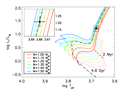
b.

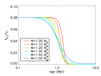
Figure 2: a. Position of the target star in the HR diagram compared with evolutionary tracks and isochrones of solar metallicity. Tracks are shown in dotted (pre-MS) and solid (main sequence onwards) colored lines; isochrones at $2$ Myr and $4.6$ Gyr are plotted as short-dashed and long-dashed black lines, respectively. b. $\mathrm{{}^{6}Li/^{7}Li}$ ratio as a function of age for the same models showing that $\mathrm{{}^{6}Li}$ is completely destroyed within approximately the first two million years of pre-MS evolution.

We adopted the values of metallicity, effective temperature, and luminosity from Table 3 of Strassmeier et al. (2011); the luminosity has been slightly revised in consideration of the new parallax now available from the first Gaia data release (Gaia Collaboration et al., 2016), which leads to smaller error bars on this quantity ($L/L_{\odot}=16.1\pm 1.3$). The best-fitting YREC track has a mass of $1.3\,M_{\sun}$, from which we derive an age of $\approx 5$ Gyr, slightly younger than the 6-7 Gyr range given by Strassmeier et al. (2011), relying on evolutionary models with core overshooting.

Our standard models predict that ⁶Li is completely destroyed early in the pre-MS, within the first two million years. As Figure 2b shows, this result is quite robust with respect to varying the stellar mass within a reasonable range.

Turning to $\mathrm{{}^{7}Li}$, we obtain $A(^{7}\rm Li)\approx 1.2$ at the age of $4.6$ Gyr for the $1.3\,M_{\odot}$ model (for reference, our adopted initial isotopic lithium abundances are $A(^{6}\rm Li)=2.2$, $A(^{7}\rm Li)=3.3$; cf. Anders & Grevesse 1989). As mentioned before, the only source of mixing in our models is convection; as a consequence, our predicted lithium abundance will be larger, in general, than that obtained with models including additional sources of mixing (for example, due to rotation). The value of $\mathrm{{}^{7}Li}$ predicted by our standard models should therefore be considered as an upper limit (see Sect. 6 for further discussion of this issue).

2.3 Observations

The spectrum used for the present Li study was taken at the Canada-France-Hawaii telescope (CFHT) with the coudé echelle spectrograph (Gecko) and is the same as analyzed in Strassmeier et al. (2011). It consists of three consecutive exposures taken on one night in May 2000. The average-combined CFHT spectrum is characterized by a resolving power of R=120 000 and a peak signal-to-noise ratio (S/R) of 400:1 per resolution element. The very high quality of this spectrum allowed us to perform a detailed spectral analysis of the Li i resonance feature in terms of both abundance and $\mathrm{{}^{6}Li/^{7}Li}$ isotopic ratio.

3 Atomic and molecular data

The main difficulty in deriving atomic and isotopic lithium abundances in a star with solar-like metal content is represented by the blends arising from various atomic and molecular lines overlapping with the lithium feature. A complete laboratory atlas of the lines that populate this spectral region around 670.8 nm still does not exist. An example for possible artifacts is the fictitious line at 670.8025 nm, first noted in the solar spectrum by Müller et al. (1975), and subsequently attributed to different elements by different authors without reaching a definite conclusion. It is thus of general interest to identify an optimal line list that is able to fit satisfactorily the lithium doublet together with the blends from the other chemical species.

We address this idea by analyzing HD 123351 with four lists of blending lines, some of which have been previously used in lithium-related work: Reddy et al. (2002), Ghezzi et al. (2009), Meléndez et al. (2012) and Israelian (2014, priv. comm.) (hereafter R02, G09, M12 and I14, respectively). To each set of blend lines we added the lithium atomic data as elaborated by Kurucz (1995) which we simplified to 12 components that account for the full lithium isotopic and hyper-fine splitting. A table of the lines of each line list, and the list of lithium components used in this work are given in Appendix A. The damping parameters were taken from the VALD-v3 database (Kupka et al., 2011).

Figure 3 visualizes the main differences between the four line lists. We plot the individual line contributions, computed separately for each element, so that their influence can be compared with the resulting full Li blend (dotted black line in Fig. 3). For this exercise, we adopted model A from Table 1 for all four panels, that is, the 3D-NLTE synthetic Li-line profile (magenta in Fig. 3 for $A$(Li) = 1.65 and $\mathrm{{}^{6}Li/^{7}Li}$ = 0.082), and 3D-LTE profiles of the blend lines (color coded for each element). We note the different line identifications in the red wing of the Li doublet where the blends interfere with the $\mathrm{{}^{6}Li}$ components.

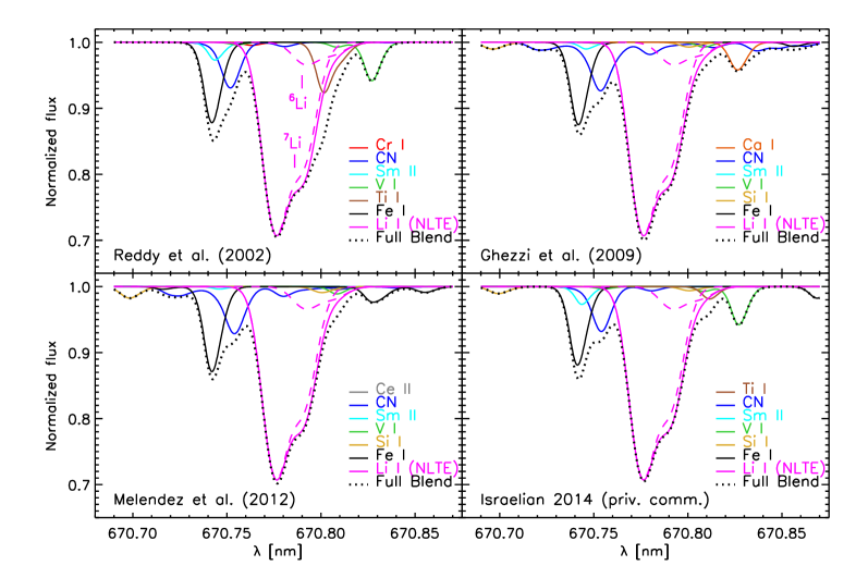
Figure 3: Visualization of the four line lists used for the grid of synthetic Li line profiles (flux). Each chemical species is synthesized in 3D separately and shown in a different color for easy identification. We adopted model A of Table 1 with parameters closest to what was found by Strassmeier et al. (2011). The lithium line (magenta, dashed lines showing the contributions due to $\mathrm{{}^{6}Li}$ and $\mathrm{{}^{7}Li}$) is computed in NLTE, whereas we assumed LTE for the blend lines. The full blend is shown as the dotted black line. No further broadening, except the 3D hydro-velocity field arising from the convective motions, has been applied to the spectra. The line lists differ in wavelength positions and $\log gf$-values, and in some cases even in the chemical element assigned to a particular line, especially in the critical red wing of the Li doublet where the $\mathrm{{}^{6}Li}$ components lie.

4 Stellar atmospheres and spectrum synthesis

4.1 3D CO⁵BOLD and 1D LHD model atmospheres

We utilized a sub-set from the CIFIST 3D hydrodynamical model atmosphere grid (Ludwig et al., 2009) computed with the CO⁵BOLD code (Freytag et al., 2012), specifically tailored around the stellar parameters of HD 123351. These models are summarized in Table 1. The adopted values of ${T_{\rm eff}}$, $\log g$ , and [Fe/H] of model A are in accordance with what was derived by Strassmeier et al. (2011), whereas models B and C allow us to estimate the sensitivity of the derived $A$(Li) and $\mathrm{{}^{6}Li/^{7}Li}$ ratio to ${T_{\rm eff}}$ and $\log g$ of the input model atmosphere. For each of these models, we also computed the corresponding 1D LHD model (Caffau & Ludwig, 2007) (labeled as a, b, and c respectively). In addition to the stellar parameters of the CO⁵BOLD models, the LHD models also share the micro-physics (opacity table, equation-of-state) and the numerics involved in treating the radiative-transfer. As such, these 1D models are differentially comparable to the related 3D hydrodynamical models.

Table 1: List of 3D CO⁵BOLD models and associated 1D LHD model atmospheres used for the analysis of HD 123351.

Model name	Label	Type	${T_{\rm eff}}$	$\log g$	$\mathrm{[Fe/H]}$	Box size	Geom. size	#	#
			[K]	cgs	dex	X$\times$Y$\times$Z	X$\times$Y$\times$Z [Mm]	Snaps	Bins
d3t48g32mm00n01	A	3D	4777$\pm$10	3.20	0.00	200${}^{2}\times$140	109.7${}^{2}\times$35.2	20	5
t4780g32mm00a05cifist	a	1D LHD	4780	3.20	0.00	–	–	–	5
d3t46g32mm00n01	B	3D	4583$\pm$13	3.20	0.00	200${}^{2}\times$140	109.7${}^{2}\times$35.2	22	5
t4580g32mm00a05	b	1D LHD	4580	3.20	0.00	–	–	–	5
d3gt46g35n03	C	3D	4552$\pm$10	3.50	0.00	200${}^{2}\times$140	109.7${}^{2}\times$35.2	12	5
t4550g35mm00ml3a05	c	1D LHD	4550	3.50	0.00	–	–	–	5

In Fig. 4, we show the thermal structure of the model atmospheres, including the uppermost part of the underlying stellar convection zone. The temperature structure of the adopted 3D model A is plotted as a probability-density distribution in orange, while the 1D LHD models with three different mixing-length parameters ($\mathrm{\alpha_{MLT}}$) are shown as solid lines, and the averaged $\langle\mathrm{3D}\rangle$ model as a dashed line. The latter is the result of a temporal and horizontal average of all the snapshots of the 3D model over surfaces of equal Rosseland optical depth. By definition, this 1D model represents the average temperature structure $\langle T^{4}(\tau_{\rm ROSS})\rangle^{1/4}$ of the 3D model. Significant temperature deviations exist especially in the subphotospheric layers ($\tau_{\rm ROSS}>1$) where the role of $\mathrm{\alpha_{MLT}}$ becomes relevant for the LHD models, leading to considerable temperature differences between the LHD model with $\mathrm{\alpha_{MLT}=0.5}$ and the $\langle\mathrm{3D}\rangle$ atmosphere.

In the photosphere ($\tau_{\rm ROSS}\leq 1$), the temperature structures of the three LHD models are indistinguishable and almost perfectly coincide with the $\langle\mathrm{3D}\rangle$ model. As we shall see in the next section, this is the line forming region of the Li resonance line in HD 123351, for which the choice of the mixing-length parameter is thus completely irrelevant. In the 1D spectrum synthesis, we therefore fix the efficiency of convection arbitrarily to $\mathrm{\alpha_{MLT}=0.5}$, keeping in mind that adopting any other value would not affect the derived $A$(Li) and $\mathrm{{}^{6}Li/^{7}Li}$ isotopic ratio.

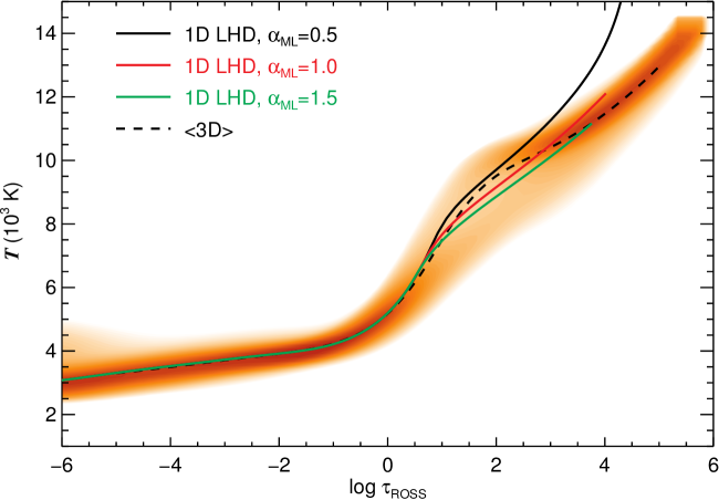
Figure 4: Temperature structure of our 3D and 1D models on the Rosseland optical depth scale $\tau_{\mathrm{ROSS}}$. The adopted 3D model A (Table 1) is shown as a probability density distribution (orange). The $\langle\mathrm{3D}\rangle$ mean model is obtained by averaging the 20 snapshots of the 3D model over surfaces of equal Rosseland optical depth (black dashed line). The three 1D LHD models with $\alpha_{\mathrm{MLT}}=0.5$ (black), $1.0$ (red), and $1.5$ (green) are shown as solid lines. The 3D model reveals photospheric temperature fluctuations in layers of fixed $\tau_{\mathrm{ROSS}}$ of several $100$ K (darker shaded regions are indicative of more likely temperatures).

4.2 3D and 1D NLTE spectrum synthesis

For each model and line list, a grid of synthetic spectra has been computed with the package Linfor3D (Steffen et al., 2015) for a predefined sample of $A$(Li) and $\mathrm{{}^{6}Li/^{7}Li}$ values, covering the wavelength range [670.69 – 670.87] nm.

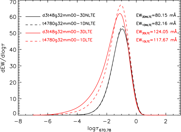
Figure 5: Equivalent-width flux contribution function for the Li I resonance line. Shown are the results for the 1D LHD model a (dashed curves, black for NLTE, red for LTE) and for the full 3D model A (interpolated to a common $\log\tau_{\mathrm{cont}}$ scale at 670.8 nm, solid curves). The lithium abundance is set to $A\rm(Li)=1.70$, and the parameter $\alpha_{\mathrm{MLT}}$ of the LHD model is 0.5.

The micro-turbulence parameter required for the 1D line formation has been derived from a set of Fe i lines in the CFHT spectrum, such that any correlation between reduced 1D-LTE equivalent widths and iron abundances measured from these lines is eliminated. For HD 123351 we found the value $\mathrm{\xi_{micro}=1.42}$ $\mathrm{km\leavevmode\nobreak\ s}^{-1}$ , which has been adopted in the 1D spectrum synthesis. The rotational profile was applied afterwards by adopting the fixed value of $v\sin i$=1.8 $\mathrm{km\leavevmode\nobreak\ s}^{-1}$ for both 3D and 1D fits (Sect. 4.3).

The lithium line formation was treated in non-LTE, using a grid of departure coefficients precomputed for each Li abundance with the code NLTE3D. The code relies on an upgraded version of the Li model atom developed by Cayrel et al. (2007) and described in Sbordone et al. (2010). Our updated model atom consists of 17 energy levels and accounts for 34 bound-bound radiative transitions. For a few test cases, we compared the results obtained with this model atom to those obtained with an even more recent lithium model atom, with 26 levels and 96 radiative transitions (see details in Klevas et al., 2016), and did not find any appreciable differences in the line profiles. We therefore decided to proceed with the already initialized computation of the grid of synthetic spectra for HD 123351 with the 17 level model atom.

Cayrel et al. (2007) showed that NLTE effects are particularly important for the lithium line formation in metal-poor stars where they strongly reduce the height range of line formation such that the Li 3D NLTE equivalent width (EW) is reduced by a factor of two compared to the 3D LTE case. For the stellar parameters of HD 123351, the NLTE effects are smaller but still substantial. Over-ionization of the ground level and, to a somewhat lesser extent, of the first excited level of the Li i resonance line is the dominant NLTE effect. The reduced line opacity and increased line source function, relative to the LTE case, both lead to a weakening of the line. The magnitude of the (positive) NLTE abundance correction is very similar in 1D and 3D ($\sim$ 0.2 dex) and is in good agreement with the results of Lind et al. (2009).

A useful way to check the impact of NLTE line formation is to compare the so-called equivalent-width Contribution Function (CF) in LTE and NLTE. This also allows us to clarify at which depth in the stellar atmosphere specific spectral lines are being formed; CF$(\tau)$ gives the relative contribution of each atmospheric layer to the equivalent width of the line.

For the 3D CO⁵BOLD model A (Table 1) and the corresponding 1D LHD model, synthetic spectra were computed for the Li feature only, assuming both LTE and NLTE. In addition to synthetic line profiles, Linfor3D also provides the equivalent-width flux CF, following the formalism described in Magain (1986). Figure 5 illustrates the result for the Li i $\lambda$ 670.8 nm line, assuming a logarithmic lithium abundance of $A$(Li)=1.70 dex according to the 1D-NLTE value derived by Strassmeier et al. (2011). The CF is constructed in units of d$\mathrm{EW}$/d$\log\tau$ over the continuum optical depth ($\log\tau_{\rm cont}$) scale at 670.8 nm, such that the integration of the curve over $\log\tau_{\rm cont}$ gives the total equivalent width of the line. In this way, the CF allows an immediate estimate of the strength of the lithium line in HD 123351 together with an indication at which atmospheric depth the line is formed.

If we consider the range of optical depth including, say, 80% of the contribution function as the line forming region, we may conclude that the lithium resonance line is mainly formed between $-3<\log\tau_{\mathrm{cont}}<0$ in NLTE. In the LTE case, there are some layers above the stellar surface that contribute more to the formation of the lithium line, causing the CF to move slightly higher in the atmosphere. This causes an increase of the EW of the Li i line of roughly 55% from 80.15 mÅ in NLTE, to 124.05 mÅ in LTE using the 3D hydrodynamical model. A similar change in EW is appreciated using 1D model atmospheres, for which neglecting departures from LTE leads to an EW that is 43% larger with respect to the NLTE assumption. In NLTE, the overall shapes of the CFs in 1D and 3D are quite similar among each other, and we expect that 3D effects in HD 123351 have only a small (but non-negligible) impact on the EW of the lithium line. However, the point of using 3D synthetic spectra is that the intrinsic shape of the 3D line profiles are supposedly more realistic (slightly asymmetric) than in 1D (intrinsically symmetric). We thus emphasize that the combined 3D NLTE effect, which can alter not only the strength but also the shape and wavelength shift of a spectral profile by appreciable amounts, should be taken into account in the determination of reliable isotopic lithium abundances.

For synthesizing the blend lines in the lithium region, we have to assume LTE, lacking the capabilities to take into account non-LTE effects for the heavier elements with more complex atomic structures. We argue, however, that non-LTE effects of the blend lines are second-order corrections that have only a minor impact on the analysis of the Li profile.

The abundance of all metals (excluding Li) is assumed to be solar according to Grevesse & Sauval (1998), except for C, N, and O, for which we adopted the values recommended by Asplund et al. (2005). A detailed abundance analysis of the relevant chemical elements based on recently observed SOPHIE spectra is presented in Appendix B.1. The results shown in Table 9 confirm that the chemical composition of HD 123351 is consistent with the adopted solar abundance mix.

4.3 Fitting procedure

We derived the lithium abundance $A$(Li) and the $\mathrm{{}^{6}Li/^{7}Li}$ isotopic ratio by fitting the CFHT spectrum of HD 123351 with synthetic spectra obtained by interpolation from the pre-computed grid of synthetic Li line profiles. For this purpose, we employ the least-squares fitting algorithm MPFIT (Markwardt, 2009) (implemented as an Interactive Data Language (IDL) routine described in more detail in Steffen et al. 2015). It adjusts iteratively four fitting parameters until the best fit (minimum $\chi^{2}$) is achieved. The set of free parameters includes $A$(Li), $\mathrm{{}^{6}Li/^{7}Li}$, a global wavelength adjustment ($\Delta v$), and a global Gaussian line broadening ($FWHM$), which are applied in velocity space to the synthetic interpolated line profile to match the observational data as closely as possible. $FWHM$ represents the full width half maximum of the applied Gaussian kernel and, in the 3D case, it includes the instrumental broadening plus an additional broadening which might have been missing from the fixed rotational broadening of $v\sin i=1.8$ $\mathrm{km\leavevmode\nobreak\ s}^{-1}$. In the 1D case, it also includes the fudge parameter known as macroturbulence that is omitted in the 3D case where both micro and macro velocity fields are already provided by the 3D model atmospheres. We relied on the original normalization of the CFHT spectrum, fixing the level of the continuum ($clevel$) to 1.00 throughout the fitting procedure.

We fit the Li doublet using two different wavelength windows:

• Full range. It covers the full synthesized spectral region between 670.69 and 670.87 nm, including all the lines belonging both to lithium and to the blends of each particular line list.

• Li range. It excludes from the fit the majority of the blends located outside the Li line (which are instead only included in the Full range). This restricted range ($\approx$ 670.76 – 670.82 nm) is helpful in understanding to what extent the blend lines beyond the Li feature, in particular the dominant Fe i line at 670.74 nm, are responsible for any change in the resulting $A$(Li) and $\mathrm{{}^{6}Li/^{7}Li}$ ratio.

5 Results

5.1 Evaluation of ${}^{6}Li/^{7}Li$ isotopic ratio

We performed the $\chi^{2}$ analysis described in Sect. 4.3 to find the best fit between the observed CFHT spectrum and the interpolated synthetic spectra for the whole set of model atmospheres (Table 1), line lists (Fig. 3), and different fitting setups (Full, Li range). Focusing on the resulting $A$(Li) and $\mathrm{{}^{6}Li/^{7}Li}$ ratio, we firstly found that, among the four line lists, R02 was not able to reproduce correctly the lithium line profile of HD 123351 using any of the fitting setups and model atmospheres, leading in general to overall bad-quality fits and even negative values for the $\mathrm{{}^{6}Li/^{7}Li}$ ratio. A negative content of $\mathrm{{}^{6}Li}$ would mean that the synthetic line profile is too depressed at the wavelength position of this isotope ($\approx$ 670.81 nm), indicating a likely erroneous blend around the $\mathrm{{}^{6}Li}$ line in R02. Referring to Fig. 3 this blend is obviously the relatively strong line of Ti i, which is absent or dramatically weaker in the other line lists for which a better agreement with the data is found.

We plot in Fig. 6 the results for the isotopic ratios derived with all combinations of models and the three remaining line lists. The 3D model atmospheres are shown in the left half of the figure and the respective 1D LHD models in the right half. The quality of each fit is expressed by the reduced $\mathrm{\chi^{2}_{red}}$ in the lower panel.

Figure 6: Results of the analysis of the lithium resonance doublet in the CFHT spectrum of HD 123351. The upper panel shows the $\mathrm{{}^{6}Li/^{7}Li}$ ratio for each line list derived with 3D CO⁵BOLD and 1D LHD model atmospheres (left and right part respectively). The model parameters are indicated on the bottom axis. Different symbols correspond to different fitting ranges; squares for the Full range, stars for the Li range. The error bars are the formal 1$\sigma$ internal fitting errors on the free parameter $\mathrm{{}^{6}Li/^{7}Li}$ and do not indicate the final uncertainty of the measurement. The quality of each fit is shown in the lower panel where the bars represent the reduced $\chi^{2}$ value.

Proving or disproving the detection of an isotope of very low abundance, such as $\mathrm{{}^{6}Li}$ in a solar metallicity star, is a delicate task which requires a pondered discussion. Referring to Fig. 6, we can summarize the following findings.

• Using model A, we detect $\mathrm{{}^{6}Li}$ with all three line lists. Its value ranges between 7% and 13% in 3D, depending on the adopted list of blend lines and fitting range.

• With the 1D LHD models, we find $\mathrm{{}^{6}Li/^{7}Li}$ to be systematically slightly larger than in the 3D case. As suggested by Cayrel et al. (2007) (see also Steffen et al., 2010), this is imputable to the fact that the asymmetry arising from convective motions is not modeled in 1D, for which reason more $\mathrm{{}^{6}Li}$ is needed to reproduce the correct asymmetric line profile. Because of the more realistic treatment of the convection, the results from 3D models are considered to be more reliable.

• The option of fitting the Li range only (star symbols) provides, in most cases, a $\mathrm{{}^{6}Li/^{7}Li}$ ratio up to 3% larger than for the Full range (squares). This is an important effect caused by the Fe i line at 670.74 nm. This line does not directly affect the lithium doublet in HD 123351 like, for example, a spurious blend; it rather intervenes, when included in the fitting range, in shifting the synthetic profile towards the red to better match the full blend, reducing the $\mathrm{{}^{6}Li}$ content needed to reproduce the asymmetry. The $\mathrm{\chi^{2}_{red}}$ obtained in fitting the Full range is considerably larger due to the fact that the blends outside the Li range (especially the dominant Fe i line) are not well fitted.

• The line list of M12 seems to be the most suitable in fitting the full doublet region of HD 123351, providing $A\rm(Li)=1.69\leavevmode\nobreak\ dex$ and $\rm{}^{6}Li/^{7}Li=10.56\leavevmode\nobreak\ \%$ using the model A with parameters closest to what was found by Strassmeier et al. (2011). Model B gives a fit of comparable quality but finds a lithium abundance that is 0.25 dex lower, as expected for the lower ${T_{\rm eff}}$ of this model.

• Using the line list of I14, we note a clear decline of $\mathrm{{}^{6}Li/^{7}Li}$ towards the models with lower ${T_{\rm eff}}$  both in 3D and in 1D. This is due to the fact that the temperature sensitive Ti i line, located close to the position of the $\mathrm{{}^{6}Li}$ isotope (see Fig. 3), is stronger with the cooler models B and C, leading to a smaller $\mathrm{{}^{6}Li}$ content. This blend is not present in M12 and G09, that both provide better fits (lower $\mathrm{\chi^{2}_{red}}$), suggesting that the Ti i blend in I14 is probably incorrect. However, should this line identification prove to be correct, it would make a reliable detection of $\mathrm{{}^{6}Li}$ in cool solar-type stars extremely challenging.

5.2 Updated $\log gf$ value for the V i line at 670.81 nm

Recently, Lawler et al. (2014) provided improved values of both oscillator strength and wavelength for, among the others, the V i line that lies very close to one of the $\mathrm{{}^{6}Li}$ components and is present in all the line lists considered in this work (see Fig. 3). These new parameters ($\lambda=670.81096$ nm, $\log gf=-2.63$) are significantly different from the values in the lists of blends available in the literature and used in this work. Depending on the line list considered, the new oscillator strength is 0.3 to 0.5 dex larger (cf.  Tables in Appendix A).

To investigate how this affects our $\mathrm{{}^{6}Li}$ detection in HD 123351, we updated the wavelength and $\log gf$ value of the V i line with the new measurements of Lawler et al. (2014) in all of our line lists. After fully re-computing the grids of synthetic 1D and 3D NLTE spectra with the modified line lists, we proceeded with fitting the CFHT spectrum as described in Sect. 4.3. The results of the best fits obtained with model atmospheres A and a (Table 1) and line lists G09, M12, and I14, are presented in Table 2, together with the results derived with the original line lists for direct comparison.

Table 2: Results of the NLTE best fits to the CFHT spectrum adopting the 3D model A and the 1D LHD model a, the line lists of Ghezzi et al. (2009), Meléndez et al. (2012), Israelian (priv. comm. 2014), and the two versions of the V i line at $\sim$670.81 nm.

Original V i line - Full range
	3D model A			1D model a
	G09	M12	I14	G09	M12	I14
$A$(Li)	1.688	1.689	1.701	1.671	1.672	1.683
$\mathrm{{}^{6}Li/^{7}Li}$	11.352	10.556	6.964	11.898	11.065	8.354
$\mathrm{\chi^{2}_{red}}$	15.178	12.082	22.828	10.590	5.898	15.589
V i line from Lawler et al. (2014) - Full range
	3D model A			1D model a
	G09	M12	I14	G09	M12	I14
$A$(Li)	1.685	1.687	1.698	1.668	1.670	1.680
$\mathrm{{}^{6}Li/^{7}Li}$	7.816	7.984	3.624	8.889	8.863	5.523
$\mathrm{\chi^{2}_{red}}$	15.578	11.856	23.827	10.961	5.669	16.358

As expected, a stronger contribution from the V i blend at this critical wavelength position has the natural effect of decreasing the amount of $\mathrm{{}^{6}Li}$ needed to best fit the data. For the line lists G09 and I14, the change in $\log gf$ is roughly $+0.5$ dex with respect to the original oscillator strength, and has the effect of lowering the lithium isotopic ratio by up to $\sim$3.5 percentage points. For M12, the smaller difference in the oscillator strength ($\Delta\log gf$ $=$ $+0.3$ dex) leads to a $\mathrm{{}^{6}Li/^{7}Li}$ ratio which is lower by 2.6 (2.2) percentage points in 3D (1D). Due to the vicinity of this V i line to one of the $\mathrm{{}^{6}Li}$ components, its impact on the $\mathrm{{}^{6}Li/^{7}Li}$ ratio is non-negligible. On the other hand, the lithium abundances $A$(Li) obtained with the modified V i line are basically unchanged for the three lists of blend lines. We also note that the modified line list M12 is still the best choice to reproduce the lithium doublet region around 670.8 nm, as indicated by the $\mathrm{\chi^{2}_{red}}$ values listed in Table 2, while the update of the V i line does not significantly improve the quality of each best fit.

a.                                                                                 b.

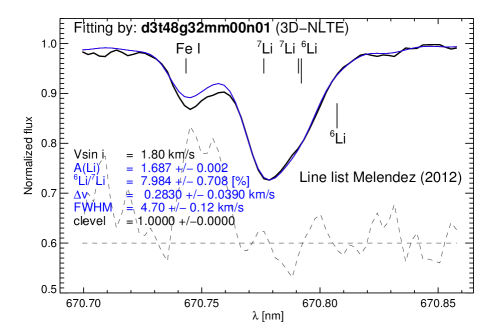
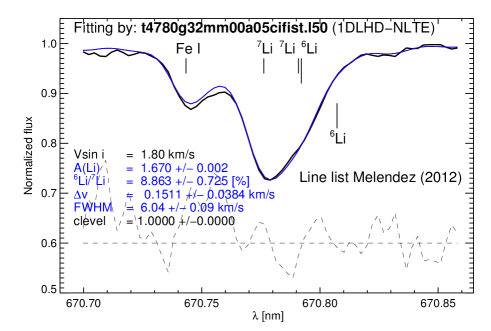
Figure 7: Best fit (thin blue line) to the CFHT spectrum (black line) obtained with line list M12+L14 in the Full range setup. (a): The fit with the 3D NLTE model A and (b): the respective 1D NLTE fit with model a. The four free parameters controlled during the fit are highlighted in the plot legend in blue, whereas $v\sin i$ and the level of the continuum were kept fixed. The residuals (dashed lines) are enhanced by a factor of ten for better visibility, and offset by $+0.6$ units in flux. The uncertainties are the formal 1$\sigma$ internal fitting errors for the given S/R = 400 of the CFHT spectrum.

Table 3: Results with the line list of M12+L14 in the Full range setup, using 3D model A and 1D LHD model a.

Models (A) and (a) - Full range			$\sigma_{\mathrm{T_{eff}}}$	$\sigma_{\mathrm{\log g}}$	$\sigma_{\mathrm{[Fe/H]}}$	$\sigma_{\mathrm{fit}}$	$\sigma_{\mathrm{blend}}$	$\sigma_{\mathrm{cont.}}$
3D-NLTE	$A$(Li)	1.687$\pm$0.114	0.111	0.018	0.010	0.002	0.007	0.012
	$\mathrm{{}^{6}Li/^{7}Li}$ [%]	7.984$\pm$4.431	0.124	1.228	2.811	0.708	2.338	2.060
1D-NLTE	$A$(Li)	1.670$\pm$0.116	0.114	0.017	0.010	0.002	0.007	0.007
	$\mathrm{{}^{6}Li/^{7}Li}$ [%]	8.863$\pm$4.108	0.015	1.177	3.121	0.725	1.853	1.338

5.3 Best fit

We cross checked the quality of our fits by visual inspection of the interpolated synthetic spectra. This, in turn, allows us to better understand the source of the magnitude of the $\mathrm{\chi^{2}_{red}}$. It is particularly useful when comparing 3D and 1D results. In Fig. 7 we show the results obtained with the list of atomic data by M12+L14 (= M12 with the V i line corrected according to Lawler et al. 2014) and model A, which best fits the lithium region around 670.8 nm, as indicated by the $\mathrm{\chi^{2}_{red}}$ in Table 2 and in the lower panel of Fig 6.

Panels (a) and (b) of Fig. 7 show the best fit from the 3D and the 1D LHD models, respectively, superimposed on the observed CFHT spectrum. We report the final results using the M12+L14 line list in Table 3 in the Full range setup, because including all the blends in the wavelength window is more objective than limiting the analysis to the Li part only.

The errors given in the Table consider six sources of uncertainty: $\sigma_{{T_{\rm eff}}}$ denotes the error due to systematic uncertainty in the effective temperature of the input model atmospheres of $\Delta{T_{\rm eff}}=\pm 100$ K, which is consistent with the ${T_{\rm eff}}$ error given by Strassmeier et al. (2011) ($\pm 70$ K, in their Table 3). Having access to the fitting results obtained with the 3D model B and the 1D LHD model b of Table 1, which are 200 K cooler than the master models A and a, $\sigma_{{T_{\rm eff}}}$ is defined as the semi-difference of the corresponding $A$(Li) and $\mathrm{{}^{6}Li/^{7}Li}$ ratio, respectively. Similarly, $\sigma_{\log g}$ and $\sigma_{\rm[Fe/H]}$ are the errors due to a variation of the surface gravity by $\Delta\log g=\pm 0.15$ dex and of the metallicity by $\Delta\rm[Fe/H]=\pm 0.10$ dex, respectively. The internal fitting error (shown as error bars in Fig. 6) is $\sigma_{\rm fit}$, whereas $\sigma_{\rm blend}$ is the error estimate related to the uncertainty of the blend modeling (which is the standard deviation of $A$(Li) and $\mathrm{{}^{6}Li/^{7}Li}$, respectively, predicted by line lists G09, M12, and I14). Finally, $\sigma_{\rm cont}$, the error related to the uncertainty of continuum placement, is defined as the semi-difference between the results obtained when treating the continuum level as a fixed and a free fitting parameter, respectively. These statistically independent contributions are summed up in quadrature to produce the final error bars given in the third column of Table  3.

Our best estimates of the lithium abundance, $\mathrm{A(Li)_{3D-NLTE}}=1.69\pm 0.11$ dex and $\mathrm{A(Li)_{1D-NLTE}}=1.67\pm 0.12$ dex, are both in excellent agreement with the earlier determination by Strassmeier et al. (2011) ($1.70\pm 0.05$ dex) based on equivalent widths. A considerable $\mathrm{{}^{6}Li}$ content is detected using both 3D and 1D models with values of 8.0 $\pm$ 4.4% (3D-NLTE) and 8.9 $\pm$ 4.1% (1D-NLTE). The similarity of these isotopic ratios indicates that the 3D effects are relatively small for HD 123351, as expected from the discussion in Sect. 4.2.

Some uncertainty remains with the dominant Fe i + CN feature at 670.74 nm that causes the enhancement in $\mathrm{\chi^{2}_{red}}$ when including this line in the fitting range. Curiously, for this line the 1D fit shows a slightly better agreement with the data (see Fig. 7). We believe that this is not related to the quality of the 3D model, but either to a 1D calibrated $\log gf$ value of this line or to a possible uncertainty in the metallicity of this star.

We demonstrate in Appendix B.2 that a slight increase of the C and/or N abundance leads to an almost perfect fit of the Fe i + CN feature without significantly changing the derived atmospheric $\mathrm{{}^{6}Li}$ content of HD 123351.

6 Discussion

As shown by Strassmeier et al. (2011), and confirmed in Sect. 2.2, our target star, HD 123351, has a mass of about 1.2–1.3 solar masses and is located on the lower part of the red giant branch, probably experiencing its first dredge-up. In this phase of evolution, it is expected to show only a very low lithium abundance at the surface, since the lithium that survived during the main-sequence evolution is diluted by a large factor when the convective envelope deepens along the lower RGB. At the same time, the temperature at the base of the outer convection zone increases to values above $2.5\times 10^{6}$ K, which leads to further destruction of lithium due to nuclear burning, even in standard models without extra mixing. For solar metallicity, the first dredge-up reduces the lithium abundance by roughly a factor of $100$ with respect to its value at the end of the main sequence (e.g., Sackmann & Boothroyd, 1999, Fig. 5).

Since our best model of HD 123351 has an age of approximately $4.5$ Gyr, its lithium abundance can be meaningfully compared to that observed in members of the open cluster M67, whose age is $\approx$ $4$ Gyr (e.g., Demarque et al. 1992; see also Barnes et al. 2016), provided that only members in an appropriate evolutionary phase are considered, that is, subgiants and/or red giant branch stars.

In Figure 8, our star is positioned in the color magnitude diagram (CMD) of M67, where cluster members have been color-coded according to their Li abundance (based on data from Pace et al. 2012). It is clear from this diagram that, in this cluster, a lithium abundance of $A\rm(^{7}Li)\lesssim 1.0$ is typical of stars that have evolved past the main sequence turnoff and populate the red giant branch. This is also in reasonably good agreement with the results of our standard model discussed in Section 2.2, where we have argued that the abundance of $A\rm(Li)=1.2$ dex predicted for our star should be interpreted as an upper limit.

With this background, it is rather surprising that we find a relatively high lithium abundance of $A$(Li) $\approx$ 1.7 in the photosphere of this star. Apparently, this result calls for a non-standard source of Li production. In the following, we discuss possible lithium production mechanisms which may explain the high content of $\mathrm{{}^{7}Li}$ and $\mathrm{{}^{6}Li}$ found in HD 123351.

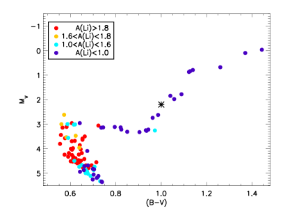
Figure 8: CMD of M67 (circles, data from Pace et al. 2012), together with HD 123351 (asterisk). The symbols representing cluster members are color-coded to reflect their lithium abundance.

6.1 Cameron-Fowler mechanism

As mentioned in the Introduction, the synthesis of fresh lithium can occur in low-mass red giants via the so-called Cameron & Fowler (1971) $\rm{}^{7}Be$ transport mechanism, if a sufficiently effective deep circulation connects the convective envelope with the hydrogen-burning shell in the stellar interior, as demonstrated by Sackmann & Boothroyd (1999). In the layers that are hot enough to support partial p-p processing, beryllium is produced by the nuclear reaction $\rm{}^{3}He(\alpha,\gamma)^{7}Be$. If mixing is fast enough, part of the ⁷Be is carried away by the circulation towards cooler regions before the $pp2$ chain can complete. Subsequently, beryllium is converted to $\mathrm{{}^{7}Li}$ by electron capture in a cooler environment where temperatures are too low for burning $\mathrm{{}^{7}Li}$. Finally, convection efficiently distributes the fresh lithium throughout the convective envelope, whereby it finally reaches the surface layers including the stellar photosphere.

In this context, it is worth recalling that HD 123351 has a binary companion in a highly eccentric orbit, which may be responsible for enhanced tidal interaction during periastron. This, in turn, may provide the physical mechanism inducing the deep circulation required for the Cameron-Fowler process to work.

Although this scenario represents a viable way to explain the presence of a considerable amount of $\mathrm{{}^{7}Li}$ in HD 123351, the Cameron-Fowler mechanism produces only $\mathrm{{}^{7}Li}$ and no $\mathrm{{}^{6}Li}$. In view of the rather high $\mathrm{{}^{6}Li/^{7}Li}$ isotopic ratio of $\approx 8\%$ derived in this work, it appears unlikely that the Cameron-Fowler mechanism is the source of Li in our target star.

6.2 Stellar flares

Another source of $\mathrm{{}^{6}Li}$ and $\mathrm{{}^{7}Li}$ production, occurring in the atmospheric layers of stars, is represented by low energy spallation reactions with C, N, and O in stellar flares (Fowler et al. 1955, Canal 1974, Canal et al. 1975, Pallavicini et al. 1992). The Sun itself seems to be producing some lithium in flares, as suggested by measurements of the $\mathrm{{}^{6}Li/^{7}Li}$ ratio in the solar wind obtained by analyzing the lunar soil ($\rm{}^{6}Li/^{7}Li\approx 3\%$, Chaussidon & Robert 1999). According to Ramaty et al. (2000), solar flares produce much more $\mathrm{{}^{6}Li}$ than $\mathrm{{}^{7}Li}$ through the ³He induced reaction ⁴He(³He,p)⁶Li. Assuming that the bulk of the $\mathrm{{}^{6}Li}$ created in the flares at the solar surface is transported away by flares or by coronal mass ejections, they find an order-of-magnitude agreement with the $\mathrm{{}^{6}Li/^{7}Li}$ measurement in the solar wind.

Even if not all the $\mathrm{{}^{6}Li}$ is expected to be carried away from the atmosphere, but is partly retained by the photospheric layers of the Sun, this contribution would not be detectable by spectroscopic observations, since the additional lithium is quickly diluted within the mass of the convective envelope: if a large solar flare produces $10^{30}$ $\mathrm{{}^{6}Li}$ atoms, of which 10% are deposited in the photosphere, it would take an enormous number of $10^{14}$ flare events to produce a detectable signature in the solar spectrum. In this sense, the scenario proposed by Ramaty et al. (2000) is also in agreement with the fact that no $\mathrm{{}^{6}Li}$ is measured in the photosphere of the Sun.

The most energetic flaring phenomena are known as superflares and have been investigated in a sample of 34 solar-type stars by Honda et al. (2015). They found that flares can occur not only in very young pre-MS objects, where the enhanced rotation and the activity tend to generate superflares, but also in older stars with lower $v\sin i$. However, they could not find any empirical evidence of lithium production by such superflares and no contribution to the $\mathrm{{}^{6}Li}$ isotope at all. Other authors have reported a strengthening of the lithium line at $\lambda$ 670.8 nm during flares in stars other than the Sun, together with an increased $\mathrm{{}^{6}Li/^{7}Li}$ ratio (Montes & Ramsey 1998, Flores Soriano et al. 2015). Clearly, more observations of such phenomena are needed to understand whether or not flares are a viable site for producing substantial amounts of lithium in stars.

In the context of Population II stars ($M_{\ast}\approx 0.8$ M_⊙), it was estimated by Tatischeff & Thibaud (2007) that the accumulated effect of flare activity during the evolution along the main sequence (MS; $\approx 10$ Gyr) can yield significant amounts of $\mathrm{{}^{6}Li}$ (and $\mathrm{{}^{7}Li}$). Under favorable assumptions, the $\mathrm{{}^{6}Li}$ concentration may reach detectable levels of ⁶Li/H $\approx 10^{-11}$ after several Gyrs of MS evolution. Although for such reasons the lithium production via stellar flares is also possible in solar-metallicity stars (the nuclear reaction rate is independent of metallicity), it is impossible to explain the amount of $\mathrm{{}^{6}Li}$ (and $\mathrm{{}^{7}Li}$) detected in HD 123351 as being a result of flare production. This is simply because the mass of the convection zone of this star ($M_{\rm CZ}\approx 1$ M_⊙) is larger by orders of magnitude compared that of the metal-poor halo stars considered by Tatischeff & Thibaud (2007). Therefore, even though HD 123351 is a particularly active star, it appears very unlikely that the lithium detected in its atmosphere is a result of flare production.

6.3 Accretion of rocky material

Another possible scenario for explaining the $\mathrm{{}^{6}Li}$ content presented in this work is linked to the external lithium enrichment being a consequence of the ingestion of planets, rocky material, or brown dwarfs that have preserved their initial lithium. This scenario was first proposed by Alexander (1967) considering evolved red giant stars and afterwards taken up by Israelian et al. (2001) to explain the $\mathrm{{}^{6}Li}$ content of the metal-rich solar-type star HD 82943 (Israelian et al., 2003). Melendez et al. (2016) studied the solar-twin star HIP 68468 hosting a 26 $\rm M_{\oplus}$ planet orbiting close to the star, suggesting some planetary migration from its original position. With an estimated age of 6 Gyr and a NLTE lithium abundance of $1.52\pm 0.03$ dex, this target can be classified as a good example of lithium enrichment due to planetary ingestion. In this framework, Melendez et al. (2016) estimated that a planet with 6 $\rm M_{\oplus}$ is necessary to reproduce the measured lithium abundance, which is higher than expected for the evolutionary stage of their target star.

In principle, a similar event could have occurred in HD 123351 when it expanded during its ascent along the RGB. The advantage of this scenario is that it would explain the observed (nearly meteoritic) $\mathrm{{}^{6}Li/^{7}Li}$ isotopic ratio of about $8$%, assuming that the total observed Li content is of planetary origin. However, we realize that the required amount of accreted planetary matter is enormous, since the mass of the convective envelope of HD 123351 is estimated to be about one solar mass (containing $\approx$ $10^{57}$ hydrogen particles) at its present stage of evolution. To explain the observed $A$(Li) $\approx$ 1.7, a total of $5\times 10^{46}$ Li particles or $5\times 10^{23}$ g of Li would need to be supplied by the external source. Assuming that the fractional lithium abundance of rocky material is $1.6\times 10^{-6}$ (McDonough, 2001), this corresponds to $3\times 10^{29}$ g or $\approx$ $53$ Earth masses of rocky material. An additional constraint is that the material must have been ingested recently (during the last few $100$ Myrs), since any previously accreted lithium would have been destroyed in the meantime by nuclear reactions at the base of the expanding convective envelope.

In view of these tight constraints, the hypothesis of planet engulfment or accretion of rocky material appears very unlikely. It is even possible that the accretion mechanism would not lead to the desired Li enrichment, but to an additional destruction of lithium (see Deal et al., 2015).

6.4 Spurious ⁶Li detection

Even though we performed the spectroscopic analysis of the Li feature with great care and attention, we cannot entirely rule out the possibility that our detection of $\mathrm{{}^{6}Li}$ in HD 123351 is spurious. For example, a weak blend that is assigned a too small $\log gf$ value (or is simply missing) in all of the line lists would be compensated by an artificial amount of $\mathrm{{}^{6}Li}$. A case in point is the V i line discussed in Sect. 5.2.

Moreover, we recall that HD 123351 is a heavily spotted star that harbors surface magnetic fields of considerable strength. The related physics is so far ignored in our model atmospheres and line formation calculations. Taking these additional complications into account might lead to subtle changes in the synthetic line profiles and to different values of the derived $\mathrm{{}^{6}Li}$ abundance. In particular, it is conceivable that the surface magnetic fields affect the Li feature through Zeeman broadening. In this case, our non-magnetic models would spuriously overestimate the abundance of $\mathrm{{}^{6}Li}$ to compensate for the missing Zeeman broadening.

7 Conclusions

We performed a full 3D NLTE analysis of the lithium resonance line at 670.8 nm in a high-resolution CFHT spectrum of the magnetically active RGB star HD 123351. We derived the lithium abundance $A$(Li) and the $\mathrm{{}^{6}Li/^{7}Li}$ isotopic ratio using different fitting techniques, model atmospheres, and a sample of blend line lists with atomic and molecular data available in the literature. Particularly good fits of the wavelength region bracketing the Li doublet were achieved with the line list of Meléndez et al. (2012), modified to account for the new $\log gf$ value measured by Lawler et al. (2014). It provides the best fit solution $\mathrm{A(Li)_{3D-NLTE}}$ = 1.69 $\pm$ 0.11 dex and $\rm{}^{6}Li/^{7}Li$ = 8.0 $\pm$ 4.4% with a 3D model atmosphere whose parameters are in accordance with the earlier analysis by Strassmeier et al. (2011), ${T_{\rm eff}}$/$\log g$/[Fe/H] = 4780/3.20/0.00. The error bars include different sources of systematic uncertainty, ensuring the robustness of our result. On the other hand, the older line list of Reddy et al. (2002) seems to include erroneous blends that lead to non-physical results in terms of a negative $\mathrm{{}^{6}Li/^{7}Li}$ ratio in HD 123351. The relatively high $\mathrm{{}^{6}Li/^{7}Li}$ isotopic ratio agrees with the values found in the solar-neighborhood interstellar medium (e.g., Lemoine et al. 1995) but challenges standard stellar evolution theory, which predicts a much lower $\mathrm{{}^{7}Li}$ abundance and the absence of $\mathrm{{}^{6}Li}$ in an RGB star that experiences the first dredge-up.

We have discussed a number of scenarios that might explain the remarkable isotopic lithium abundances found in this evolved target. The Cameron-Fowler mechanism could explain the relatively high $\mathrm{{}^{7}Li}$ abundance of HD 123351, where the required extra mixing might be provided by tidal interaction during periastron passage of the binary companion. However, this scenario cannot account for the presence of $\mathrm{{}^{6}Li}$. A possible source of $\mathrm{{}^{6}Li}$ production is represented by low energy spallation reactions in stellar flares. Even though our target star is known for its high level of magnetic activity, it appears unlikely that a sufficient amount of $\mathrm{{}^{6}Li}$ can be produced by this mechanism. The planet engulfment hypothesis would naturally explain the essentially meteoritic $\mathrm{{}^{6}Li/^{7}Li}$ isotopic ratio, but would require the recent accretion of about 50 Earth masses of rocky material.

This work underlines the need for improved atomic and molecular data to establish a complete and reliable identification of the various blends at the position of the $\mathrm{{}^{6}Li}$ isotopic absorption line. The present work relies on published lists of blend lines that have previously been used in Li-related work, with some modification accounting for recently updated atomic data for a critical V i line. In contrast to the total Li abundance $A$(Li), the derived $\mathrm{{}^{6}Li/^{7}Li}$ isotopic ratio depends critically on the details of the blending lines. A weak blend missing in these line lists might easily lead to a substantial downward revision of the derived $\mathrm{{}^{6}Li/^{7}Li}$ isotopic ratio.

In a follow-up paper, we plan to analyze very high resolution PEPSI spectra of HD 123351 to verify the Li isotopic abundances derived in the present work from a CFHT spectrum. The PEPSI spectra will also allow us to derive the $\mathrm{{}^{12}C/^{13}C}$ isotopic ratio to better constrain the evolutionary state of HD 123351. In addition, the PEPSI observations will give us the opportunity to study the spectrum of the target at different epochs.

Appendix A Atomic and molecular data

Tables 4, 5, 6, and 7 present the list of atomic and molecular data adopted for synthesizing the lithium doublet region. The Li transitions accounting for hyper-fine splitting and isotopic shifts are listed in Table 8.

Table 4: Line list by Reddy et al. (2002).

Reddy et al. (2002)
Wavelength	Chemical	Excitation	log $gf$
$\lambda$ (Å)	species	potential (eV)	(dex)
6707.381	CN	1.830	-2.170
6707.433	Fe i	4.607	-2.283
6707.450	Sm ii	0.930	-1.040
6707.464	CN	0.792	-3.012
6707.521	CN	2.169	-1.428
6707.529	CN	0.956	-1.609
6707.529	CN	2.009	-1.785
6707.529	CN	2.022	-1.785
6707.563	V i	2.743	-1.530
6707.644	Cr i	4.207	-2.140
6707.740	Ce ii	0.500	-3.810
6707.752	Ti i	4.050	-2.654
6707.771	Ca i	5.796	-4.015
6707.816	CN	1.206	-2.317
6708.025	Ti i	1.880	-2.252
6708.094	V i	1.220	-3.113
6708.125	Ti i	1.880	-2.886
6708.280	V i	1.218	-2.178
6708.375	CN	2.100	-2.252

Table 5: Line list by Ghezzi et al. (2009).

Ghezzi et al. (2009)
Wavelength	Chemical	Excitation	log $gf$
$\lambda$ (Å)	species	potential (eV)	(dex)
6706.980	Si i	5.954	-2.797
6707.205	CN	1.970	-1.222
6707.282	CN	2.040	-1.333
6707.371	CN	3.050	-0.522
6707.431	Fe i	4.608	-2.268
6707.457	CN	0.790	-3.055
6707.470	CN	1.880	-1.451
6707.473	Sm ii	0.933	-1.477
6707.518	V i	2.743	-1.995
6707.545	CN	0.960	-1.548
6707.595	CN	1.890	-1.851
6707.596	Cr i	4.208	-2.767
6707.645	CN	0.960	-2.460
6707.740	Ce ii	0.500	-3.810
6707.752	Sc i	4.049	-2.672
6707.771	Ca i	5.796	-4.015
6707.807	CN	1.210	-1.853
6707.848	CN	3.600	-2.417
6707.899	CN	3.360	-3.110
6707.930	CN	1.980	-1.651
6707.964	Ti i	1.879	-6.903
6707.980	CN	2.390	-2.027
6708.023	Si i	6.000	-2.910
6708.026	CN	1.980	-2.031
6708.094	V i	1.218	-3.113
6708.147	CN	1.870	-1.434
6708.275	Ca i	2.710	-3.377
6708.375	CN	1.979	-1.097
6708.499	CN	1.868	-1.423
6708.577	Fe i	5.446	-2.728
6708.635	CN	1.870	-1.584

Table 6: Line list by Meléndez et al. (2012).

Melendez et al. (2012)
Wavelength	Chemical	Excitation	log $gf$
$\lambda$ (Å)	species	potential (eV)	(dex)
6707.000	Si i	5.954	-2.560
6707.172	Fe i	5.538	-2.810
6707.205	CN	1.970	-1.222
6707.272	CN	2.177	-1.416
6707.282	CN	2.055	-1.349
6707.300	C2	0.933	-1.717
6707.371	CN	3.050	-0.522
6707.433	Fe i	4.608	-2.250
6707.460	CN	0.788	-3.094
6707.461	CN	0.542	-3.730
6707.470	CN	1.880	-1.581
6707.473	Sm ii	0.933	-1.910
6707.548	CN	0.946	-1.588
6707.595	CN	1.890	-1.451
6707.596	Cr i	4.208	-2.667
6707.645	CN	0.946	-3.330
6707.660	C2	0.926	-1.743
6707.809	CN	1.221	-1.935
6707.848	CN	3.600	-2.417
6707.899	CN	3.360	-3.110
6707.930	CN	1.980	-1.651
6707.970	C2	0.920	-1.771
6707.980	CN	2.372	-3.527
6708.023	Si i	6.000	-2.800
6708.026	CN	1.980	-2.031
6708.094	V i	1.218	-2.922
6708.099	Ce ii	0.701	-2.120
6708.147	CN	1.870	-1.884
6708.282	Fe i	4.988	-2.700
6708.315	CN	2.640	-1.719
6708.347	Fe i	5.486	-2.580
6708.370	CN	2.640	-2.540
6708.420	CN	0.768	-3.358
6708.534	Fe i	5.558	-2.936
6708.541	CN	2.500	-1.876
6708.577	Fe i	5.446	-2.684

Table 7: Line list by Israelian (2014, priv. comm.).

Israelian (2014, priv. comm.)
Wavelength	Chemical	Excitation	log $gf$
$\lambda$ (Å)	species	potential (eV)	(dex)
6707.010	Si i	5.954	-2.784
6707.381	CN	1.830	-2.170
6707.426	Fe i	4.610	-2.293
6707.450	Sm ii	0.930	-1.040
6707.464	CN	0.792	-3.012
6707.521	CN	2.169	-1.428
6707.551	CN	0.956	-1.609
6707.551	CN	2.009	-1.785
6707.551	CN	2.022	-1.785
6707.563	V i	2.743	-1.530
6707.604	Cr i	4.208	-2.410
6707.740	Ce ii	0.500	-3.810
6707.752	Ti i	4.050	-2.654
6707.771	Ca i	5.800	-4.015
6707.816	CN	1.206	-2.317
6708.025	Si i	6.000	-2.970
6708.094	V i	1.218	-3.113
6708.125	Ti i	1.880	-2.886
6708.280	V i	1.220	-2.178
6708.375	CN	2.100	-2.252
6708.700	Fe i	4.220	-3.658

Table 8: The twelve components ($\mathrm{{}^{7}Li}$ and $\mathrm{{}^{6}Li}$) representing the lithium hyper-fine structure (HFS) and isotopic shifts, regrouped from the original sample of 19 components given by Kurucz (1995).

Lithium HFS
Wavelength	Lithium	Excitation	log $gf$
$\lambda$ (Å)	isotope	potential (eV)	(dex)
6707.756	$\mathrm{{}^{7}Li}$	0.000	-0.428
6707.768	$\mathrm{{}^{7}Li}$	0.000	-0.206
6707.907	$\mathrm{{}^{7}Li}$	0.000	-0.808
6707.908	$\mathrm{{}^{7}Li}$	0.000	-1.507
6707.919	$\mathrm{{}^{7}Li}$	0.000	-0.808
6707.920	$\mathrm{{}^{7}Li}$	0.000	-0.808
6707.920	$\mathrm{{}^{6}Li}$	0.000	-0.479
6707.923	$\mathrm{{}^{6}Li}$	0.000	-0.178
6708.069	$\mathrm{{}^{6}Li}$	0.000	-0.831
6708.070	$\mathrm{{}^{6}Li}$	0.000	-1.734
6708.074	$\mathrm{{}^{6}Li}$	0.000	-0.734
6708.075	$\mathrm{{}^{6}Li}$	0.000	-0.831

Appendix B The chemical composition of HD 123351

B.1 Abundance analysis of SOPHIE spectra

We verified the chemical composition of the star by analyzing three spectra observed with the SOPHIE spectrograph mounted at the 1.93 m telescope of the Observatory de Haute-Provence. Two spectra were observed on 28.01.2009 (S09) and 05.03.2014 (S14) at high efficiency (resolving power $R$ $\sim$ $40\,000$) and one was taken on 21.01.2017 (S17) at high spectral resolution ($R$ $\sim$ $75\,000$).

Table 9: Solar chemical composition used for the spectrum synthesis (Col. 2) and chemical abundances of available elements (Col. 7) derived with MyGIsFOS from three SOPHIE spectra (S09, S14, S17). Columns (4)–(6) give the number of lines analyzed of each spectrum.

Chemical composition HD 123351
Element	$A\rm(X)_{\odot}$	Ionization	N lines			$A\rm(X)_{\star}$
	[dex]	stage	S09	S14	S17	[dex]
C	8.39	I	1	1	1	$8.46\pm 0.15$
N	7.80	-	-	-	-	-
O	8.66	I	-	-	1	$8.60\pm 0.10$
Si	7.55	I	5	-	6	$7.49\pm 0.13$
Ca	6.36	I	1	1	-	$6.38\pm 0.15$
Sc	3.17	I	4	4	4	$3.22\pm 0.10$
Ti	5.02	I	11	9	4	$4.88\pm 0.10$
V	4.00	I	3	3	2	$3.95\pm 0.10$
Cr	5.67	I	3	3	3	$5.62\pm 0.15$
Fe	7.50	I	63	60	44	$7.44\pm 0.10$
Ce	1.58	-	-	-	-	-
Sm	1.01	-	-	-	-	-

Individual chemical abundances were derived with the automated analysis pipeline MyGIsFOS (Sbordone et al. 2014), assuming the stellar parameters ${T_{\rm eff}}=4780$ K, $\log g=3.2$, and $\xi_{\rm micro}=1.4$ $\mathrm{km\leavevmode\nobreak\ s}^{-1}$. We report the resulting abundances of importance for the blends in the Li range in Table 9. The carbon abundance of $A({\rm C})=8.46\pm 0.15$ is based on the analysis of a single atomic line at 538.0 nm. We also investigated the G-band, but could not determine a reliable carbon abundance from this molecular band because the CH lines are saturated and the region is contaminated by saturated atomic lines, which makes the definition of the continuum difficult. The oxygen abundance of $A({\rm O})=8.60\pm 0.10$ is derived from the forbidden [OI] line. Unfortunately, we could not derive a nitrogen abundance since the relevant atomic lines are located in the infrared, outside the SOPHIE spectral range.

Nevertheless, for all the major elements whose lines are present in the various blends around the lithium doublet, our chemical analysis indicates that, within the error bars, the metallicity of this star is consistent with a solar chemical composition, thus confirming the value of $\rm[Fe/H]=0.00\pm 0.08$ obtained by Strassmeier et al. (2011). We also confirm that their stellar parameters, adopted in this work, yield an optimal consistency of excitation and ionization equilibria.

Throughout this work, we used the CIFIST2006 solar abundances (Col. 2 of Table 9) as the input chemical composition for the spectrum synthesis calculations. The above analysis shows that this choice is fully justified.

B.2 Fine-tuning the fit of the Fe i + CN blend

As discussed in Section 5.3, the quality of the fit of the dominant Fe i + CN blend around $\lambda\,670.74$ nm is relatively poor. Here we describe some further tests to investigate to what extent an improved fit of this feature would affect our $\mathrm{{}^{6}Li}$ detection in HD 123351.

From the best fits shown in Fig. 7, it is obvious that some opacity is missing in the vicinity of the Fe i+CN blend at $\lambda\,670.74$ nm. Considering the line list M12 with the updated V i line at $\lambda\,670.81$ nm, we additionally experimented with changing the $\log gf$ value of the dominant Fe i line at $\lambda\,670.7433$ nm. We recomputed the grid of 1D NLTE synthetic spectra, increasing $\log gf$ of this particular line by different amounts. Following this procedure, a reasonable fit of the Fe i feature was achieved with $\Delta\log gf$ $=$ $+0.07$ dex. At the same time, the best fit required a significant redshift of the whole synthetic spectrum. This effect was expected, as previously discussed in Section 5, and leads to a reduction of the $\mathrm{{}^{6}Li/^{7}Li}$ isotopic ratio by about 2.6 percentage points with respect to the values listed in Table 2. However, we also noticed that increasing the strength of the Fe i line could not fully compensate for some missing opacity near the position of the CN blend. Even though the overall fit of the Full range is significantly improved by enhancing the Fe i absorption, the fit to the lithium line profile (Li range) deteriorates. Therefore, we looked for an alternative solution.

As clearly shown in Fig. 3, the CN blend at 670.755 nm should not to be considered less important than the dominant iron line, since it contributes significantly to the opacity on the blue part of the Li i doublet. Manipulating the $\log gf$ values of the CN band is not as convenient as for the Fe i case, since there are several CN lines in this region. We instead applied some small changes in carbon abundance $A\rm(C)$. Considering the line list M12 with the updated V i line and recomputing once again the grid of 1D NLTE synthetic spectra with different $A$(C), we found a best fit assuming $A\rm(C)=8.45$ (Fig. 9). This carbon abundance is $0.06$ dex larger than the solar value ($A\rm(C)$ $=$ $8.39$) adopted in all our previous spectrum synthesis calculations, and perfectly in agreement with the carbon abundance derived from the atomic line at $\lambda\,538.0$ nm (Appendix B.1). Alternatively, the same result is obtained when increasing the abundance of both carbon and nitrogen by $0.04$ dex.

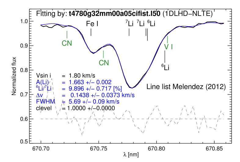
Figure 9: 1D NLTE best-fit of the CFHT spectrum using the 1D LHD model a of Table 1 and the list of atomic and molecular data M12, modified to account for the new $\log gf$ value measured by Lawler et al. (2014) for the V i blend line. For the synthetic spectra, we assumed an enhancement in $A$(C) by $+0.06$ dex with respect to the solar value. The wavelength positions of the V i line and of the main contribution to the CN band are indicated in green.

With this fine-tuning of the carbon abundance, we were not only able to improve the fit of the CN feature ($\lambda$670.755 nm, see Fig. 9) but also to match the nearby Fe i feature almost perfectly. The improvement of the fit is a consequence of the fact that by adjusting the CN blend, the required broadening, expressed by the free parameter $FWHM$, is lower, leading to a narrower iron feature which naturally reproduces the observed data. With this slight change of the chemical setup, the measured $\mathrm{{}^{6}Li/^{7}Li}$ ratio is hardly affected (increasing from $8.9$ to $9.9$%), corroborating our previous results.

This analysis could in principle be repeated in 3D NLTE, but with a much higher computational cost. From Fig. 7 (panel $a$) it appears that in 3D the opacity missing is larger than in 1D. Presumably, a 3D fit of the same quality as achieved in 1D would require a slight adjustment of both the $\log gf$ value of the Fe i line and an increase of the C and/or N abundance, with all changes well within the uncertainties. Extrapolating from the 1D experience, it seems reasonable to say that the $\mathrm{{}^{6}Li/^{7}Li}$ ratio is only marginally affected by the fine-tuning of the Fe i + CN blend, thus leaving our 3D NLTE $\mathrm{{}^{6}Li}$ detection of $\approx 8$% unchallenged.