ADMM Penalty Parameter Selection by Residual Balancing

Abstract

Appropriate selection of the penalty parameter is crucial to obtaining good performance from the Alternating Direction Method of Multipliers (ADMM). While analytic results for optimal selection of this parameter are very limited, there is a heuristic method that appears to be relatively successful in a number of different problems. The contribution of this paper is to demonstrate that their is a potentially serious flaw in this heuristic approach, and to propose a modification that at least partially addresses it.

I Introduction

The Alternating Direction Method of Multipliers (ADMM) has become a very popular approach to solving a broad variety of optimization problems in signal and image processing, prominent examples including Total Variation regularization and sparse representation problems [1], [2, Sec. 6],  [3]. This method introduces an additional parameter, the penalty parameter, on which the rate of convergence is strongly dependent, but for which there are no analytic results to guide selection other than for a very specific set of problems [4, 5], [6, Sec. 5]. There is, however, a heuristic method for automatically adapting the penalty parameter [7] that appears to becoming quite popular [8, 9, 10, 11, 12, 13]. The present paper demonstrates a serious flaw in this heuristic approach, and proposes a modification that at least partially addresses it.

II ADMM

The notation and exposition in this section follows that of the influential tutorial by Boyd et al. [2]. The Lagrangian for the constrained problem

$$\operatorname*{arg\,min}_{\mathbf{x}}f(\mathbf{x})\;\text{ such that }\;A\mathbf{x}=\mathbf{b}\;,$$ (1)

is

$$L(\mathbf{x},\mathbf{y})=f(\mathbf{x})+\mathbf{y}^{T}(A\mathbf{x}-\mathbf{b})\;,$$ (2)

where $\mathbf{x}$ and $\mathbf{y}$ are referred to as the primal and dual variables respectively. The primal and dual feasibility conditions

$$0=\nabla L(\mathbf{x}^{*},\cdot)\;\;\Rightarrow\;\; A\mathbf{x}^{*}-\mathbf{b}=0$$ (3)

$$0\in\partial L(\cdot,\mathbf{y}^{*})\;\;\Rightarrow\;\; 0\in\partial f(\mathbf{x}^{*})+A^{T}\mathbf{y}^{*}\;,$$ (4)

where $\partial$ denotes the subdifferential operator [14, Ch. D], provide conditions on the optimal primal and dual variables $\mathbf{x}^{*}$ and $\mathbf{y}^{*}$. The method of multipliers solves this problem via dual ascent

$$\mathbf{x}^{(k+1)} =\operatorname*{arg\,min}_{\mathbf{x}}L_{\rho}(\mathbf{x},\mathbf{y}^{(k)})$$ (5)

$$\mathbf{y}^{(k+1)} =\mathbf{y}^{(k)}+\rho(A\mathbf{x}^{(k+1)}-\mathbf{b})\;,$$ (6)

where $L_{\rho}$ is the augmented Lagrangian

$$L_{\rho}(\mathbf{x},\mathbf{y})=f(\mathbf{x})+\mathbf{y}^{T}(A\mathbf{x}-\mathbf{b})+\frac{\rho}{2}\left\|A\mathbf{x}-\mathbf{b}\right\|_{2}^{2}$$ (7)

with penalty parameter $\rho$.

ADMM can be viewed as a variant of this method applied to the problem

$$\operatorname*{arg\,min}_{\mathbf{x},\mathbf{z}}f(\mathbf{x})+g(\mathbf{z})\;\text{ such that }\;A\mathbf{x}+B\mathbf{z}=\mathbf{c}\;,$$ (8)

where $\mathbf{x}\in\mathbb{R}^{n}$, $\mathbf{z}\in\mathbb{R}^{m}$, and $\mathbf{c}\in\mathbb{R}^{p}$, and the Lagrangian and augmented Lagrangian are, respectively,

$$L(\mathbf{x},\mathbf{z},\mathbf{y})= f(\mathbf{x})+g(\mathbf{z})+\mathbf{y}^{T}(A\mathbf{x}+B\mathbf{z}-\mathbf{c})$$ (9)

$$L_{\rho}(\mathbf{x},\mathbf{z},\mathbf{y})= L(\mathbf{x},\mathbf{z},\mathbf{y})+\frac{\rho}{2}\left\|A\mathbf{x}+B\mathbf{z}-\mathbf{c}\right\|_{2}^{2}\;.$$ (10)

Instead of jointly solving for $\mathbf{x}$ and $\mathbf{z}$, ADMM alternates the $\mathbf{x}$ and $\mathbf{z}$ updates (thus the alternating direction)

$$\mathbf{x}^{(k+1)} =\operatorname*{arg\,min}_{\mathbf{x}}L_{\rho}(\mathbf{x},\mathbf{z}^{(k)},\mathbf{y}^{(k)})$$ (11)

$$\mathbf{z}^{(k+1)} =\operatorname*{arg\,min}_{\mathbf{z}}L_{\rho}(\mathbf{x}^{(k+1)},\mathbf{z},\mathbf{y}^{(k)})$$ (12)

$$\mathbf{y}^{(k+1)} =\mathbf{y}^{(k)}+\rho(A\mathbf{x}^{(k+1)}+B\mathbf{z}^{(k+1)}-\mathbf{c})\;.$$ (13)

It is often more convenient to work with the scaled form of ADMM, which is obtained by the change of variable to the scaled dual variable $\mathbf{u}=\rho^{-1}\mathbf{y}$. Defining the residual

$$\mathbf{r}=A\mathbf{x}+B\mathbf{z}-\mathbf{c}$$ (14)

and replacing $\mathbf{y}$ with $\mathbf{u}$ we have

$$L_{\rho}(\mathbf{x},\mathbf{z},\mathbf{u}) =f(\mathbf{x})+g(\mathbf{z})+\frac{\rho}{2}\left\|\mathbf{r}+\mathbf{u}\right\|_{2}^{2}-\frac{\rho}{2}\left\|\mathbf{u}\right\|_{2}^{2}\;.$$ (15)

Since the minimisers of $L_{\rho}(\mathbf{x},\mathbf{z},\mathbf{u})$ with respect to $\mathbf{x}$ and $\mathbf{z}$ do not depend on the final $\frac{\rho}{2}\left\|\mathbf{u}\right\|_{2}^{2}$ term, the iterations can be written as

$$\mathbf{x}^{(k+1)} =\operatorname*{arg\,min}_{\mathbf{x}}f(\mathbf{x})+\frac{\rho}{2}\left\|A\mathbf{x}+B\mathbf{z}^{(k)}-\mathbf{c}+\mathbf{u}^{(k)}\right\|_{2}^{2}$$ (16)

$$\mathbf{z}^{(k+1)} =\operatorname*{arg\,min}_{\mathbf{z}}g(\mathbf{z})+\frac{\rho}{2}\left\|A\mathbf{x}^{(k+1)}+B\mathbf{z}-\mathbf{c}+\mathbf{u}^{(k)}\right\|_{2}^{2}$$ (17)

$$\mathbf{u}^{(k+1)} =\mathbf{u}^{(k)}+A\mathbf{x}^{(k+1)}+B\mathbf{z}^{(k+1)}-\mathbf{c}\;.$$ (18)

II-A ADMM Residuals

Denote optimal primal variables by $\mathbf{x}^{*}$ and $\mathbf{z}^{*}$, and the optimal dual variable by $\mathbf{y}^{*}$. It will also be useful to define $p^{*}=f(\mathbf{x}^{*})+g(\mathbf{z}^{*})$ and $p^{(k)}=f(\mathbf{x}^{(k)})+g(\mathbf{z}^{(k)})$. The primal feasibility condition

$$A\mathbf{x}^{*}+B\mathbf{z}^{*}-\mathbf{c}=0\;,$$ (19)

and dual feasibility conditions

$$0\in\partial L(\cdot,\mathbf{z}^{*},\mathbf{y}^{*})\;\Rightarrow\;\; 0\in\partial f(\mathbf{x}^{*})+A^{T}\mathbf{y}^{*}$$ (20)

$$0\in\partial L(\mathbf{x}^{*},\cdot,\mathbf{y}^{*})\;\Rightarrow\;\; 0\in\partial g(\mathbf{z}^{*})+B^{T}\mathbf{y}^{*}$$ (21)

for Eq. (8) hold at the problem solution $(\mathbf{x}^{*},\mathbf{z}^{*},\mathbf{y}^{*})$. These conditions can be used to derive convergence measures for ADMM algorithm iterates $(\mathbf{x}^{(k)},\mathbf{z}^{(k)},\mathbf{y}^{(k)})$.

A natural measure of primal feasibility based on Eq. (19) is the primal residual

$$\mathbf{r}^{(k+1)}=A\mathbf{x}^{(k+1)}+B\mathbf{z}^{(k+1)}-\mathbf{c}\;.$$ (22)

Now, since $\mathbf{z}^{(k+1)}$ minimises $L_{\rho}(\mathbf{x}^{(k+1)},\mathbf{z},\mathbf{y}^{(k)})$ (see Eq. (12)), we have

$$0 \in[\partial L_{\rho}(\mathbf{x}^{(k+1)},\cdot,\mathbf{y}^{(k)})](\mathbf{z}^{(k+1)})$$

$$=\partial g(\mathbf{z}^{(k+1)})+B^{T}\mathbf{y}^{(k)}$$

$$\qquad\qquad\;\;\;\;\;\;\,+\rho B^{T}(A\mathbf{x}^{(k+1)}+B\mathbf{z}^{(k+1)}-\mathbf{c})$$

$$=\partial g(\mathbf{z}^{(k+1)})+B^{T}\mathbf{y}^{(k)}+\rho B^{T}\mathbf{r}^{(k+1)}$$

$$=\partial g(\mathbf{z}^{(k+1)})+B^{T}(\mathbf{y}^{(k)}+\rho\mathbf{r}^{(k+1)})$$

$$=\partial g(\mathbf{z}^{(k+1)})+B^{T}\mathbf{y}^{(k+1)}\;,$$ (23)

so that iterates $\mathbf{z}^{(k+1)}$ and $\mathbf{y}^{(k+1)}$ always satisfy dual feasibility condition Eq. (21), leaving Eq. (20) as the remaining optimality criteria to be satisfied. Following a similar derivation, since $\mathbf{x}^{(k+1)}$ minimises $L_{\rho}(\mathbf{x},\mathbf{z}^{(k)},\mathbf{y}^{(k)})$ (see Eq. (11)), we have

$$0 \in[\partial L_{\rho}(\cdot,\mathbf{z}^{(k)},\mathbf{y}^{(k)})](\mathbf{x}^{(k+1)})$$

$$=\partial f(\mathbf{x}^{(k+1)})+A^{T}\mathbf{y}^{(k)}+\rho A^{T}(A\mathbf{x}^{(k+1)}+B\mathbf{z}^{(k)}-\mathbf{c})$$

$$=\partial f(\mathbf{x}^{(k+1)})+A^{T}\mathbf{y}^{(k)}+\rho A^{T}(A\mathbf{x}^{(k+1)}+B\mathbf{z}^{(k+1)}$$

$$\qquad\qquad\qquad\qquad\qquad\;\;\;\;\;-\mathbf{c}+B\mathbf{z}^{(k)}-B\mathbf{z}^{(k+1)})$$

$$=\partial f(\mathbf{x}^{(k+1)})+A^{T}\mathbf{y}^{(k)}$$

$$\qquad\qquad\qquad+\rho A^{T}(\mathbf{r}^{(k+1)}+B\mathbf{z}^{(k)}-B\mathbf{z}^{(k+1)})$$

$$=\partial f(\mathbf{x}^{(k+1)})+A^{T}(\mathbf{y}^{(k)}$$

$$\qquad\qquad\qquad+\rho\mathbf{r}^{(k+1)})+\rho A^{T}B(\mathbf{z}^{(k)}-\mathbf{z}^{(k+1)})$$

$$=\partial f(\mathbf{x}^{(k+1)})+A^{T}\mathbf{y}^{(k+1)}\!+\!\rho A^{T}B(\mathbf{z}^{(k)}\!-\!\mathbf{z}^{(k+1)})\;.$$ (24)

Setting $\rho A^{T}B(\mathbf{z}^{(k+1)}-\mathbf{z}^{(k)})=0$ in Eq. (24) implies that $\mathbf{x}^{(k+1)},\mathbf{y}^{(k+1)}$ satisfy dual feasibility condition Eq. (20), which suggests defining

$$\mathbf{s}^{(k+1)}=\rho A^{T}B(\mathbf{z}^{(k+1)}-\mathbf{z}^{(k)})$$ (25)

as the dual residual based on dual feasibility condition Eq. (20).

Since both primal and dual residuals converge to zero as the ADMM algorithm progresses [2, Sec. 3.3], they can be used to define ADMM algorithm convergence measures. It is also worth noting that Eq. (11) and Eq. (12) suggest that the norm of the primal residual decreases with increasing $\rho$ (and vice versa), and the definition of the dual residual suggests that it increases with increasing $\rho$ (and vice versa).

II-B Adaptive Penalty Parameter

As discussed in Sec. I, the correct choice of the penalty parameter plays a vital role in obtaining good convergence. He et al. [7] define the distance from convergence as $\|\mathbf{r}^{(k+1)}\|_{2}^{2}+\|\mathbf{s}^{(k+1)}\|_{2}^{2}$, and argue that adaptively choosing the penalty parameter to balance these two terms is a reasonable heuristic for minimising this distance. This heuristic is implemented as the update scheme

$$\rho^{(k+1)}=\left\{\ \begin{array}[]{ll}\tau\rho^{(k)}&\text{ if }\big{\lVert}\mathbf{r}^{(k)}\big{\rVert}_{2}>\mu\big{\lVert}\mathbf{s}^{(k)}\big{\rVert}_{2}\\[3.0pt] \tau^{-1}\rho^{(k)}&\text{ if }\big{\lVert}\mathbf{s}^{(k)}\big{\rVert}_{2}>\mu\big{\lVert}\mathbf{r}^{(k)}\big{\rVert}_{2}\\[3.0pt] \rho^{(k)}&\text{ otherwise }\;,\end{array}\right.$$ (26)

where $\tau$ and $\mu$ are constants, the usual values being $\tau=2$ and $\mu=10$ [7, 16], [2, Sec 3.4.1].

This scheme has has been found to be effective for a variety of problems [8, 9, 10, 11, 12, 13], but it will be demonstrated that it suffers from a potentially serious flaw.

II-C Stopping Criteria

The residuals can be used to define stopping criteria for the ADMM iterations; e.g. Boyd et al. [2, Sec. 3.3.1] recommend stopping criteria

$$\big{\lVert}\mathbf{r}^{(k)}\big{\rVert}_{2}\leq\epsilon_{\mathrm{pri}}^{(k)}\;\;\text{ and }\big{\lVert}\mathbf{s}^{(k)}\big{\rVert}_{2}\leq\epsilon_{\mathrm{dua}}^{(k)}$$ (27)

where

$$\epsilon_{\mathrm{pri}}^{(k)} \!=\!\sqrt{p}\epsilon_{\mathrm{abs}}\!+\!\epsilon_{\mathrm{rel}}\max\left\{\big{\lVert}A\mathbf{x}^{(k)}\big{\rVert}_{2},\big{\lVert}B\mathbf{z}^{(k)}\big{\rVert}_{2},\big{\lVert}\mathbf{c}\big{\rVert}_{2}\right\}$$ (28)

$$\epsilon_{\mathrm{dua}}^{(k)}\! \!=\sqrt{n}\epsilon_{\mathrm{abs}}+\epsilon_{\mathrm{rel}}\big{\lVert}A^{T}\mathbf{y}^{(k)}\big{\rVert}_{2}\;,$$ (29)

$\epsilon_{\mathrm{abs}}$ and $\epsilon_{\mathrm{rel}}$ are absolute and relative tolerances respectively, and $n$ and $p$ are the dimensionalities of $\mathbf{x}$ and $\mathbf{c}$ respectively (i.e. $\mathbf{x}\in\mathbb{R}^{n}$ and $\mathbf{c}\in\mathbb{R}^{p}$).

III ADMM Problem Scaling Properties

Let us consider the behaviour of ADMM under scaling of the optimization problem being addressed, denoting Eq. (8) as problem $P$, and defining $\tilde{P}$ as

$$\operatorname*{arg\,min}_{\mathbf{x},{\mathbf{z}}}\alpha f(\gamma\mathbf{x})+\alpha g(\gamma\mathbf{z})\;\text{ s.t. }\;\beta A\gamma\mathbf{x}+\beta B\gamma\mathbf{z}=\beta\mathbf{c}\;.$$ (30)

In this problem $\alpha$ represents a scaling of the objective function, $\beta$ represents a scaling of the constraint, and $\gamma$ represents a scaling of the problem variables. These scalings are chosen to parameterise the family of scalings of an ADMM problem under which the solution is invariant, modulo a scaling. It is important to emphasise that these scalings can represent both explicit scaling of a problem and the implicit scaling with respect to alternative possible choices inherent in choosing functional, constraints, and variables. Problem $\tilde{P}$ can be expressed in the standard form as

$$\operatorname*{arg\,min}_{\mathbf{x},{\mathbf{z}}}\tilde{f}(\mathbf{x})+\tilde{g}(\mathbf{z})\;\text{ such that }\;\tilde{A}\mathbf{x}+\tilde{B}\mathbf{z}=\tilde{\mathbf{c}}$$ (31)

with

$$\tilde{f}(\mathbf{x})=\alpha f(\gamma\mathbf{x})\quad\tilde{g}(\mathbf{z})=\alpha g(\gamma\mathbf{z})\quad$$

$$\tilde{A}=\beta\gamma A\quad\tilde{B}=\beta\gamma B\quad\tilde{\mathbf{c}}=\beta\mathbf{c}\;.$$ (32)

The Lagrangian is

$$\tilde{L}({\mathbf{x}},{\mathbf{z}},{\mathbf{y}})=\alpha f(\gamma\mathbf{x}) +\alpha g(\gamma\mathbf{z})$$

$$+\mathbf{y}^{T}(\beta\gamma A\mathbf{x}+\beta\gamma B\mathbf{z}-\beta\mathbf{c})\;,$$ (33)

and the primal and dual feasibility conditions are

$$\beta A\gamma\tilde{\mathbf{x}}^{*}+\beta B\gamma\tilde{\mathbf{z}}^{*}-\beta\tilde{\mathbf{c}}=0\;,$$ (34)

and

$$0\in\partial\tilde{L}(\cdot,\tilde{\mathbf{z}}^{*},\tilde{\mathbf{y}}^{*})\;\Rightarrow\; 0\!\in\!\alpha\gamma[\partial f(\cdot)](\gamma\tilde{\mathbf{x}}^{*})+\beta\gamma A^{T}\tilde{\mathbf{y}}^{*}=0$$ (35)

$$0\in\partial\tilde{L}(\tilde{\mathbf{x}}^{*},\cdot,\tilde{\mathbf{y}}^{*})\;\Rightarrow\; 0\!\in\!\alpha\gamma[\partial g(\cdot)](\gamma\tilde{\mathbf{z}}^{*})+\beta\gamma B^{T}\tilde{\mathbf{y}}^{*}=0$$ (36)

respectively. It is easily verified that if $\mathbf{x}^{*}$, $\mathbf{z}^{*}$, and $\mathbf{y}^{*}$ satisfy the optimality criteria Eq. (19), (20), and (21) for problem $P$, then

$$\tilde{\mathbf{x}}^{*}=\gamma^{-1}\mathbf{x}^{*}\quad\;\;\tilde{\mathbf{z}}^{*}=\gamma^{-1}\mathbf{z}^{*}\quad\;\;\tilde{\mathbf{y}}^{*}=\frac{\alpha}{\beta}\mathbf{y}^{*}$$ (37)

satisfy the primal and dual feasibility criteria for $\tilde{P}$. The augmented Lagrangian for $\tilde{P}$ is

$$\tilde{L}_{\tilde{\rho}}(\mathbf{x},\mathbf{z},\mathbf{y}) =\alpha f(\gamma\mathbf{x})+\alpha g(\gamma\mathbf{z})$$

$$+\alpha\left(\frac{\beta}{\alpha}\mathbf{y}^{T}\right)(\gamma A\mathbf{x}+\gamma B\mathbf{z}-\mathbf{c})$$

$$+\alpha\left(\frac{\beta^{2}}{\alpha}\tilde{\rho}\right)\frac{1}{2}\left\|\gamma A\mathbf{x}+\gamma B\mathbf{z}-\mathbf{c}\right\|_{2}^{2}\;,$$ (38)

so that setting

$$\tilde{\rho}=\frac{\alpha}{\beta^{2}}\rho$$ (39)

gives

$$\tilde{L}_{\tilde{\rho}}(\mathbf{x},\mathbf{z},\mathbf{y})=\alpha L_{\rho}\left(\gamma\mathbf{x},\gamma\mathbf{z},\frac{\beta}{\alpha}\mathbf{y}\right)\;.$$ (40)

The iterates $\mathbf{x}^{(k+1)}$, $\mathbf{z}^{(k+1)}$, and $\mathbf{y}^{(k+1)}$ for iteration $k$ of the ADMM algorithm for $P$ are given by Eq. (11), (12), and (13). We now consider the corresponding iterates for $\tilde{P}$, assuming that

$$\tilde{\mathbf{z}}^{(k)}=\gamma^{-1}\mathbf{z}^{(k)}\quad\quad\tilde{\mathbf{y}}^{(k)}=\frac{\alpha}{\beta}\mathbf{y}^{(k)}\;.$$ (41)

The $\mathbf{x}$ update is

$$\tilde{\mathbf{x}}^{(k+1)} =\operatorname*{arg\,min}_{\mathbf{x}}\tilde{L}_{\tilde{\rho}}(\mathbf{x},\tilde{\mathbf{z}}^{(k)},\tilde{\mathbf{y}}^{(k)})$$

$$=\operatorname*{arg\,min}_{\mathbf{x}}\tilde{L}_{\tilde{\rho}}(\mathbf{x},\gamma^{-1}\mathbf{z}^{(k)},\frac{\alpha}{\beta}\mathbf{y}^{(k)})$$

$$=\operatorname*{arg\,min}_{\mathbf{x}}\alpha L_{\rho}(\gamma\mathbf{x},\mathbf{z}^{(k)},\mathbf{y}^{(k)})\;.$$ (42)

For convex $f$ we have that if $\mathbf{x}^{*}$ minimises $f(\mathbf{x})$ then $\gamma^{-1}\mathbf{x}^{*}$ minimises $\tilde{f}(\mathbf{x})=\alpha f(\gamma\mathbf{x})$, so

$$\tilde{\mathbf{x}}^{(k+1)}=\gamma^{-1}\mathbf{x}^{(k+1)}\;,$$ (43)

and similarly it can be shown that

$$\tilde{\mathbf{z}}^{(k+1)}=\gamma^{-1}\mathbf{z}^{(k+1)}\;.$$ (44)

For the $\mathbf{y}$ update we have

$$\tilde{\mathbf{y}}^{(k+1)} =\tilde{\mathbf{y}}^{(k)}+\tilde{\rho}(\beta\gamma A\tilde{\mathbf{x}}^{(k+1)}+\beta\gamma B\tilde{\mathbf{z}}^{(k+1)}-\beta\mathbf{c})$$

$$=\frac{\alpha}{\beta}\left(\mathbf{y}^{(k)}+\rho(A\mathbf{x}^{(k+1)}+B\mathbf{z}^{(k+1)}-\mathbf{c})\right)$$

$$=\frac{\alpha}{\beta}\mathbf{y}^{(k+1)}\;.$$ (45)

Finally, the primal and dual residuals for $\tilde{P}$ have the following scaling relationship with those of $P$:

$$\tilde{\mathbf{r}}^{(k+1)} =\tilde{A}\tilde{\mathbf{x}}^{(k+1)}+\tilde{B}\tilde{\mathbf{z}}^{(k+1)}-\tilde{\mathbf{c}}$$

$$=\beta A\mathbf{x}^{(k+1)}+\beta B\mathbf{z}^{(k+1)}-\beta\mathbf{c}$$

$$=\beta\mathbf{r}^{(k+1)}$$ (46)

$$\tilde{\mathbf{s}}^{(k+1)} =\tilde{\rho}\tilde{A}^{T}\tilde{B}(\tilde{\mathbf{z}}^{(k+1)}-\tilde{\mathbf{z}}^{(k)})$$

$$=\alpha\gamma\rho A^{T}B(\mathbf{z}^{(k+1)}-\mathbf{z}^{(k)})$$

$$=\alpha\gamma\mathbf{s}^{(k+1)}\;.$$ (47)

In summary, the parameters $\alpha$, $\beta$, and $\gamma$ in problem $\tilde{P}$ generate families of ADMM problems with the same solutions (modulo a scaling, in the case of $\gamma$), as expressed in Eq. (37), but the iterates of the corresponding ADMM algorithms are only similarly invariant if the initial iterates (see Eq. (41)) and constant penalty parameter (see Eq. (39)) are appropriately scaled.

IV Residual Balancing

The scaling properties described in the previous section have a major impact on the residuals and their use within the residual balancing scheme for penalty parameter selection.

IV-A Adaptive Penalty Parameter

It was demonstrated above that ADMM algorithm iterates can be made invariant to problem scaling by a suitable choice of fixed penalty parameter. It is easily verified that invariance can be maintained with a varying penalty parameter $\rho^{(k)}$ as long as the required relationship is also maintained, i.e. $\tilde{\rho}^{(k)}=\frac{\alpha}{\beta^{2}}\rho^{(k)}$. If an adaptive update rule such as Eq. (26), that operates by multiplying the penalty parameter by some factor, is to preserve this relationship, it is necessary that (i) $\tilde{\rho}^{(0)}=\frac{\alpha}{\beta^{2}}\rho^{(0)}$, and (ii) the choice of multiplier and when to apply it must be invariant to problem scaling. But it is clear from Eq. (46) and Eq. (46) that the primal and dual residuals do not share the same scaling factors, so that the update rule Eq. (26) based on these residuals does not, in general, preserve the scaling behaviour of the penalty parameter required to maintain invariance of the algorithm iterates. It follows that if the adaptive penalty parameter method of Sec. II-B performs well for some problem $P$, it should not be expected to do so for problem $\tilde{P}$ as the scaling parameters $\alpha$, $\beta$, and $\gamma$ deviate from unity.

If update rule Eq. (26) is known to provide good performance for a reference problem $P$, and it becomes necessary to modify the problem formulation in a way that corresponds to switching to a scaled problem $\tilde{P}$ (e.g. a change of physical units), then the same performance can be achieved by using a modified update rule

$$\rho^{(k+1)}=\left\{\ \begin{array}[]{ll}\tau\rho^{(k)}&\text{ if }\big{\lVert}\mathbf{r}^{(k)}\big{\rVert}_{2}>\xi\mu\big{\lVert}\mathbf{s}^{(k)}\big{\rVert}_{2}\\[3.0pt] \tau^{-1}\rho^{(k)}&\text{ if }\big{\lVert}\mathbf{s}^{(k)}\big{\rVert}_{2}>\xi^{-1}\mu\big{\lVert}\mathbf{r}^{(k)}\big{\rVert}_{2}\\[3.0pt] \rho^{(k)}&\text{ otherwise }\;,\end{array}\right.$$ (48)

with $\xi=\beta^{-1}\alpha\gamma$ chosen to compensate for the scaling of the ratio of residuals with the problem scaling.

It is important to emphasise, however, that this issue is not only relevant to the practitioner considering explicitly scaling an existing ADMM problem: problem $\tilde{P}$ merely makes explicit the implicit choices involved in setting up any ADMM problem, and there is no reason to believe that the often-arbitrary choices made in setting up the problem correspond to an optimal or even a good choice of scaling with respect to the convergence of the ADMM iterates subject to update rule Eq. (26), or subject to update rule Eq. (48) with $\xi=1$.

IV-B Relative Residuals

A simple approach that avoids the need for explicit compensation for problem scaling when the formulation is modified is to base the adaptive penalty parameter policy on residuals that represent relative instead of absolute error. If the normalisations required for relative error measures are selected appropriately, they will cancel the scaling with $\beta$ and $\alpha\gamma$, making them invariant to problem scaling. A reasonable normalisation to make the primal residual $\mathbf{r}^{(k+1)}=A\mathbf{x}^{(k+1)}+B\mathbf{z}^{(k+1)}-\mathbf{c}$ a relative residual is

$$\max\left\{\big{\lVert}A\mathbf{x}^{(k+1)}\big{\rVert}_{2},\big{\lVert}B\mathbf{z}^{(k+1)}\big{\rVert}_{2},\big{\lVert}\mathbf{c}\big{\rVert}_{2}\right\}\;,$$

allowing us to define the relative primal residual

$$\mathbf{r}_{\mathrm{rel}}^{(k+1)}=\frac{A\mathbf{x}^{(k+1)}+B\mathbf{z}^{(k+1)}-\mathbf{c}}{\max\left\{\big{\lVert}A\mathbf{x}^{(k+1)}\big{\rVert}_{2},\big{\lVert}B\mathbf{z}^{(k+1)}\big{\rVert}_{2},\big{\lVert}\mathbf{c}\big{\rVert}_{2}\right\}}\;,$$ (49)

which is invariant to problem scaling since the normalisation factor has the same scaling as the absolute residual,

$$\max\left\{\big{\lVert}\tilde{A}\tilde{\mathbf{x}}^{(k+1)}\big{\rVert}_{2},\big{\lVert}\tilde{B}\tilde{\mathbf{z}}^{(k+1)}\big{\rVert}_{2},\big{\lVert}\tilde{\mathbf{c}}\big{\rVert}_{2}\right\}\\ =\max\left\{\big{\lVert}\beta\gamma A\gamma^{-1}\mathbf{x}^{(k+1)}\big{\rVert}_{2},\big{\lVert}\beta\gamma B\gamma^{-1}\mathbf{z}^{(k+1)}\big{\rVert}_{2},\big{\lVert}\beta\mathbf{c}\big{\rVert}_{2}\right\}\\ =\beta\max\left\{\big{\lVert}A\mathbf{x}^{(k+1)}\big{\rVert}_{2},\big{\lVert}B\mathbf{z}^{(k+1)}\big{\rVert}_{2},\big{\lVert}\mathbf{c}\big{\rVert}_{2}\right\}\;.$$ (50)

A suitable normalisation for the dual residual $\mathbf{s}^{(k+1)}=\rho A^{T}B(\mathbf{z}^{(k+1)}-\mathbf{z}^{(k)})$ can be obtained from Eq. (24). When $f$ is differentiable and the gradient is easily computable, a reasonable choice of the normalisation would be $\max\left\{\big{\lVert}\nabla f(\mathbf{x}^{(k+1)})\big{\rVert}_{2},\big{\lVert}A^{T}\mathbf{y}^{(k+1)}\big{\rVert}_{2}\right\}$, but since this is often not the case, we simply use $\big{\lVert}A^{T}\mathbf{y}^{(k+1)}\big{\rVert}_{2}$ as the normalisation factor, giving the relative dual residual

which is again invariant to problem scaling since the normalisation factor has the same scaling as the absolute residual,

Using these definitions, $\tilde{\mathbf{r}}_{\mathrm{rel}}^{(k+1)}=\mathbf{r}_{\mathrm{rel}}^{(k+1)}$ and $\tilde{\mathbf{s}}_{\mathrm{rel}}^{(k+1)}=\mathbf{s}_{\mathrm{rel}}^{(k+1)}$; i.e. the residuals are invariant to problem scaling. The corresponding penalty parameter update policy becomes

$$\rho^{(k+1)}=\left\{\ \begin{array}[]{ll}\tau\rho^{(k)}&\text{ if }\big{\lVert}\mathbf{r}_{\mathrm{rel}}^{(k)}\big{\rVert}_{2}>\xi\mu\big{\lVert}\mathbf{s}_{\mathrm{rel}}^{(k)}\big{\rVert}_{2}\\[3.0pt] \tau^{-1}\rho^{(k)}&\text{ if }\big{\lVert}\mathbf{s}_{\mathrm{rel}}^{(k)}\big{\rVert}_{2}>\xi^{-1}\mu\big{\lVert}\mathbf{r}_{\mathrm{rel}}^{(k)}\big{\rVert}_{2}\\[3.0pt] \rho^{(k)}&\text{ otherwise }\;,\end{array}\right.$$ (53)

where the parameter $\xi$ is retained for reasons that will be made apparent shortly.

The convergence proof [7] of the standard adaptive scheme (i.e. Eq. (26) with the standard definitions of the residuals) depends only on bounds on the sequences $\rho^{(k)}$ and $\eta_{k}=\sqrt{(\rho^{(k+1)}/\rho^{(k)})^{2}-1}$, neither of which is affected by the change in the definition of the residuals, so the convergence results still hold under the modified definitions of the residuals.

IV-C Adaptive Multiplier Policy

The fixed multiplier $\tau$ is a potential weakness of the penalty update policies Eq. (26) and Eq. (53). If $\tau$ is small, then a large number of iterations may be required to reach an appropriate $\rho$ value if $\rho^{(0)}$ is poorly chosen (i.e., so that $\big{\lVert}\mathbf{r}^{(0)}\big{\rVert}_{2}\gg\xi\big{\lVert}\mathbf{s}^{(0)}\big{\rVert}_{2}$, or $\big{\lVert}\mathbf{r}^{(0)}\big{\rVert}_{2}\ll\xi\big{\lVert}\mathbf{s}^{(0)}\big{\rVert}_{2}$). On the other hand, if $\tau$ is large, the corrections to $\rho$ may be too large when $\rho$ is close to the optimal value.

A straightforward solution is to adapt $\tau$ at each iteration

where $\tau_{\mathrm{max}}$ provides a bound on $\tau$. Since $\tau$ is bounded, the convergence results [7] still hold for this extension.

IV-D Stopping Criteria

The stopping criteria in Sec. II-C can be expressed in terms of the relative residuals $\mathbf{r}_{\mathrm{rel}}$ and $\mathbf{s}_{\mathrm{rel}}$ as

$$\big{\lVert}\mathbf{r}_{\mathrm{rel}}^{(k)}\big{\rVert}_{2}\leq\epsilon_{\mathrm{pri}}^{(k)}\;\;\text{ and }\big{\lVert}\mathbf{s}_{\mathrm{rel}}^{(k)}\big{\rVert}_{2}\leq\epsilon_{\mathrm{dua}}^{(k)}$$ (55)

where

$$\epsilon_{\mathrm{pri}}^{(k)} \!=\!\sqrt{p}\epsilon_{\mathrm{abs}}/\max\left\{\big{\lVert}A\mathbf{x}^{(k)}\big{\rVert}_{2},\big{\lVert}B\mathbf{z}^{(k)}\big{\rVert}_{2},\big{\lVert}\mathbf{c}\big{\rVert}_{2}\right\}\!+\!\epsilon_{\mathrm{rel}}$$ (56)

$$\epsilon_{\mathrm{dua}}^{(k)}\! \!=\sqrt{n}\epsilon_{\mathrm{abs}}/\big{\lVert}A^{T}\mathbf{y}^{(k)}\big{\rVert}_{2}+\epsilon_{\mathrm{rel}}\;.$$ (57)

These stopping criteria are invariant to problem scaling when $\epsilon_{\mathrm{abs}}=0$.

IV-E Residual Ratio

While the relative residuals proposed in Sec. IV-B address the absence of scaling invariance in the adaptive penalty parameter strategy based on residual balancing, there is another even more serious deficiency that is not so easily remedied. As discussed in Sec. II-B, the target ratio of unity is motivated by representing the distance from convergence as $\|\mathbf{r}^{(k)}\|_{2}^{2}+\|\mathbf{s}^{(k)}\|_{2}^{2}$, but this greatly simplifies the true picture.

The ADMM convergence proof in [2] (see Sec. 3.3.1 and Appendix A) provides some insight into the relationship between the distance from convergence and the residuals, in the form of the inequality

$$f(\mathbf{x}^{(k)})+g(\mathbf{z}^{(k)})-p^{*}\leq\; -(\mathbf{y}^{(k)})^{T}\mathbf{r}^{(k)}$$

$$+(\mathbf{x}^{(k)}-\mathbf{x}^{*})^{T}\mathbf{s}^{(k)}\;,$$ (58)

which implies the looser inequality

$$f(\mathbf{x}^{(k)})+g(\mathbf{z}^{(k)})-p^{*}\leq\; \big{\lVert}\mathbf{y}^{(k)}\big{\rVert}\big{\lVert}\mathbf{r}^{(k)}\big{\rVert}+$$

$$\big{\lVert}\mathbf{x}^{(k)}-\mathbf{x}^{*}\big{\rVert}\big{\lVert}\mathbf{s}^{(k)}\big{\rVert}$$ (59)

in terms of the norms of the relevant vectors. Applying the original argument that led to unity as the appropriate target ratio to this inequality implies that the appropriate ratio is, in fact, approximately $\big{\lVert}\mathbf{y}^{(k)}\big{\rVert}/\big{\lVert}\mathbf{x}^{(k)}-\mathbf{x}^{*}\big{\rVert}$. This would explain why some authors have found the original residual balancing strategy of Eq. (26) to be effective [8, 9, 10, 11, 12, 13] and others have not [19, Sec. 2.4]: the method succeeds when this ratio happens to be relatively close to unity, and fails when it is not.

Unfortunately, since $\mathbf{x}^{*}$ is unknown while solving the problem, there is no obvious way to estimate this ratio, and we are left with the rather unsatisfactory solution of accepting $\xi$ in Eq. (53) as a user-selected parameter of the method. Since this approach essentially replaces one user parameter, $\rho$, with another, $\xi$, it is not clear that the residual balancing strategy has any real value as a parameter selection technique. One might argue that, since the residual balancing method has been found to be satisfactory in a variety of applications, it must often be the case that $\xi=1$ is not too far from the optimal setting, and that $\xi$ may be a more stable parameterisation than $\rho$, but further study is necessary before any reliable conclusions can be drawn.

Since Eq. (53) retains $\xi$, which can be used to compensate for explicit problem scaling as discussed in Sec. IV-A, it is reasonable to ask whether there is any real benefit to using Eq. (53) based on the relative residuals, i.e., since we have an unknown $\xi$ in both cases, what is the advantage of one scaling of this unknown quantity in comparison with another. Two arguments can be made in favour of the use of relative residuals as in Eq. (53):

• Ignoring the question of determining a good choice of $\xi$, once one has been found, Eq. (53) is invariant to problem scaling, while Eq. (26) is not.

• Since Eq. (53) is invariant to problem scaling, one might expect that the $\xi$ for this update rule is more stable than the $\xi$ for Eq. (53), in the sense that it varies across a smaller numerical range for different problem. (This important question is not explored in the experimental results presented here.)

It should also be noted that the unknown scalings of the residuals in Eq. (59) imply that neither the absolute nor relative stopping tolerances in Sec. IV-D can be viewed as providing an actual bound on the solution optimality, either in an absolute or a relative sense (e.g. a relative stopping criterion $\epsilon_{\mathrm{rel}}=10^{-3}$ does not imply that the final iterate is within $10^{-3}$ relative distance to the optimal solution).

V BPDN

To illustrate these issues, we will focus on Basis Pursuit DeNoising (BPDN) [20],

$$\operatorname*{arg\,min}_{\mathbf{x}}\frac{1}{2}\left\|D\mathbf{x}-\boldsymbol{\varsigma}\right\|_{2}^{2}+\lambda\left\|\mathbf{x}\right\|_{1}\;,$$ (60)

a standard problem in computing sparse representations corresponding to Eq. (8) with

$$f(\mathbf{x})=\frac{1}{2}\left\|D\mathbf{x}-\boldsymbol{\varsigma}\right\|_{2}^{2}\;\;\;\;g(\mathbf{z})=\lambda\left\|\mathbf{z}\right\|_{1}$$

$$A=I\;\;\;\;B=-I\;\;\;\;\mathbf{c}=0\;.$$ (61)

Solving via ADMM, we have problem $P$

$$\operatorname*{arg\,min}_{\mathbf{x}}\frac{1}{2}\left\|D\mathbf{x}-\boldsymbol{\varsigma}\right\|_{2}^{2}+\lambda\left\|\mathbf{z}\right\|_{1}\text{ s.t. }\mathbf{x}=\mathbf{z}$$ (62)

with Lagrangian

$$L(\mathbf{x},\mathbf{z},\mathbf{y})=\frac{1}{2}\left\|D\mathbf{x}-\boldsymbol{\varsigma}\right\|_{2}^{2}+\lambda\left\|\mathbf{z}\right\|_{1}+\mathbf{y}^{T}(\mathbf{x}-\mathbf{z})\;.$$ (63)

We also consider Convolutional BPDN (CBPDN), a variant of BPDN constructed by replacing the linear combination of a set of dictionary vectors by the sum of a set of convolutions with dictionary filters [21, Sec. II]

$$\operatorname*{arg\,min}_{\{\mathbf{x}_{m}\}}\frac{1}{2}\Big{\lVert}\sum_{m}\mathbf{d}_{m}\ast\mathbf{x}_{m}-\boldsymbol{\varsigma}\Big{\rVert}_{2}^{2}+\lambda\sum_{m}\left\|\mathbf{x}_{m}\right\|_{1}\;,$$ (64)

where $\{\mathbf{d}_{m}\}$ is a set of $M$ dictionary filters, $\ast$ denotes convolution, and $\{\mathbf{x}_{m}\}$ is a set of coefficient maps. Algebraically, this variant is a special case of standard BPDN, so that the same scaling properties apply, but since the dictionaries in this form are very highly overcomplete (the overcompleteness factor is equal to the number of filters $M$), one may expect that this variant might exhibit at least somewhat different behaviour in practice. A further difference is that the $\{\mathbf{x}_{m}\}$ can be efficiently computed without any factorisation of system matrices [13], so in this case the penalty update policy is applied at every iteration instead of at every 10 iterations.

VI Results

In this section the issues discussed above are illustrated via a number of computational experiments. Many of these experiments compare the effect of different penalty parameter selection methods on the number of iterations required to reach the stopping criteria. With respect to these experiments, it must be emphasised that:

• Since the relationship between the stopping criteria and the actual solution suboptimality is unknown (see Sec. IV-E), reaching the stopping criteria faster does not imply faster convergence.

• These experiments all use relative stopping thresholds (i.e. $\epsilon_{\mathrm{abs}}=0$), which could be considered to confer an advantage on the relative residual balancing policy since it balances the residuals in a way that that is favourable to satisfying the relative stopping thresholds. Note, however, that the original goal of invariance to problem scaling cannot be achieved if $\epsilon_{\mathrm{abs}}\neq 0$.

VI-A BPDN with Random Dictionary

Figure 1: A comparison of functional value evolution for the same problem with adaptive $\rho$ based on standard and normalised residuals.

Figure 2: A comparison of primal and dual residual evolution for the same problem with adaptive $\rho$ based on standard and normalised residuals. For a meaningful comparison, the residuals are divided by their respective values of $\epsilon_{\mathrm{pri}}$ or $\epsilon_{\mathrm{dua}}$.

Figure 3: A comparison of selected $\rho$ values for the same problem with adaptive $\rho$ based on standard and normalised residuals.

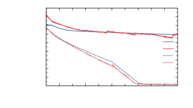
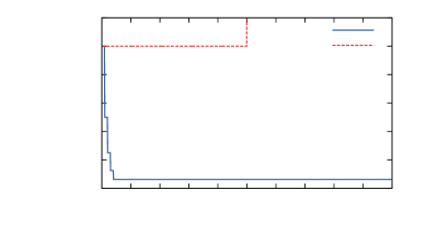
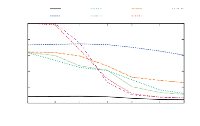
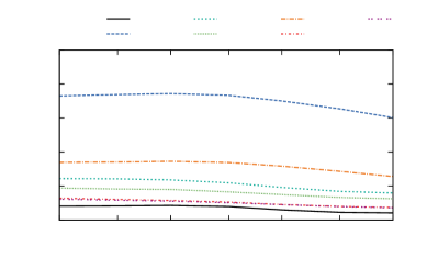
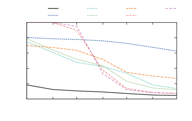
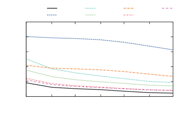
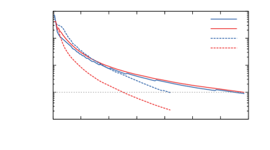
The first experiment involves sparse coefficient recovery on a random dictionary without normalisation. A dictionary $D\in\mathbb{R}^{512\times 4096}$ was generated with unit standard deviation i.i.d. entries with a Gaussian distribution, a corresponding reference coefficient vector $\mathbf{x}_{0}$ was constructed by assigning random values to 64 randomly selected coefficients, the remainder of which were zero, and a test signal was constructed by adding Gaussian white noise of standard deviation 0.5 to the product of $D$ and $\mathbf{x}_{0}$. The experiment involves using BPDN with $\lambda=40$ (selected for good support identification), $\xi=1$, $\epsilon_{\mathrm{abs}}=0$, and $\epsilon_{\mathrm{rel}}=10^{-4}$ to attempt to recover $\mathbf{x}_{0}$ from the signal, comparing performance with both standard and normalised residuals. It is clear from Figs. 1–3 that the adaptive $\rho$ policy gives very substantially better performance with normalised residuals than with the standard definition. The desired stopping tolerance is reached within 160 iterations when using normalised residuals, but has still not been attained when the maximum iteration limit of 1000 is reached in the case of standard residuals. The performance difference is even greater if random dictionary $D$ is generated with standard deviation greater than unity.

VI-B BPDN with Learned Dictionary

(a) Standard residuals

(b) Normalised residuals

Figure 4: Variation with $\rho^{(0)}$ of number of iterations required to reach a relative stopping tolerance of $\epsilon_{\mathrm{rel}}=10^{-3}$ for different variants of the adaptive $\rho$ policy, and for standard and normalised residuals, in a BPDN problem with $D\in\mathbb{R}^{64\times 128}$ and $\lambda=10^{-2}$. The variant labels are “Fixed”, indicating that $\rho$ is fixed at $\rho^{(0)}$ and is not adapted, of the form $\mu/\tau$, or of the form $\mu$/Auto, which indicates that $\tau$ is adapted as in Eq. (54), with $\tau_{\mathrm{max}}=100$ and $\xi=1$.

(a) Standard residuals

(b) Normalised residuals

Figure 5: Mean number of iterations (averaged over all values of $\rho^{(0)}$) required to reach a relative stopping tolerance of $\epsilon_{\mathrm{rel}}=10^{-3}$ for different variants of the adaptive $\rho$ policy, and for standard and normalised residuals, in a BPDN problem with $D\in\mathbb{R}^{64\times 64}$ and varying $\lambda$. The variant labels are “Fixed”, indicating that $\rho$ is fixed at $\rho^{(0)}$ and is not adapted, of the form $\mu/\tau$, or of the form $\mu$/Auto, which indicates that $\tau$ is adapted as in Eq. (54), with $\tau_{\mathrm{max}}=100$ and $\xi=1$. “Fixed (min)” denotes the minimum number of iterations (i.e. not the mean) obtained via the best fixed choice of $\rho^{(0)}$ at each value of $\lambda$.

(a) Standard residuals

(b) Normalised residuals

Figure 6: Mean number of iterations (averaged over all values of $\rho^{(0)}$) required to reach a relative stopping tolerance of $\epsilon_{\mathrm{rel}}=10^{-3}$ for different variants of the adaptive $\rho$ policy, and for standard and normalised residuals, in a BPDN problem with $D\in\mathbb{R}^{64\times 96}$ and varying $\lambda$. The variant labels are “Fixed”, indicating that $\rho$ is fixed at $\rho^{(0)}$ and is not adapted, of the form $\mu/\tau$, or of the form $\mu$/Auto, which indicates that $\tau$ is adapted as in Eq. (54), with $\tau_{\mathrm{max}}=100$ and $\xi=1$. “Fixed (min)” denotes the minimum number of iterations (i.e. not the mean) obtained via the best fixed choice of $\rho^{(0)}$ at each value of $\lambda$.

(a) Standard residuals

(b) Normalised residuals

Figure 7: Mean number of iterations (averaged over all values of $\rho^{(0)}$) required to reach a relative stopping tolerance of $\epsilon_{\mathrm{rel}}=10^{-3}$ for different variants of the adaptive $\rho$ policy, and for standard and normalised residuals, in a BPDN problem with $D\in\mathbb{R}^{64\times 128}$ and varying $\lambda$. The variant labels are “Fixed”, indicating that $\rho$ is fixed at $\rho^{(0)}$ and is not adapted, of the form $\mu/\tau$, or of the form $\mu$/Auto, which indicates that $\tau$ is adapted as in Eq. (54), with $\tau_{\mathrm{max}}=100$ and $\xi=1$. “Fixed (min)” denotes the minimum number of iterations (i.e. not the mean) obtained via the best fixed choice of $\rho^{(0)}$ at each value of $\lambda$.

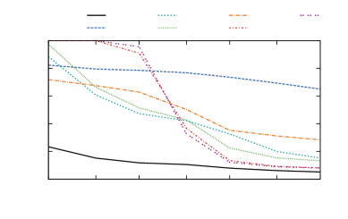
The second set of experiments compares the performance of a fixed $\rho$ and various adaptive $\rho$ parameter choices, using standard and normalised residuals, for a Multiple Measurement Vector (MMV) BPDN problem. Dictionaries $D\in\mathbb{R}^{64\times 64}$, $D\in\mathbb{R}^{64\times 96}$, and $D\in\mathbb{R}^{64\times 128}$ were learned on a large training set of $8\times 8$ image patches, and the test data consisted of 32558 zero-mean $8\times 8$ image patches represented as a matrix $S\in\mathbb{R}^{64\times 32258}$. The number of iterations required to attain a relative stopping tolerance of $\epsilon_{\mathrm{rel}}=10^{-3}$ for $D\in\mathbb{R}^{64\times 128}$ and $\lambda=10^{-2}$ is compared in Fig. 4. The following observations can be made with respect to the ability of the different methods to reduce the dependence of the number of iterations on the initial choice $\rho^{(0)}$:

• The best choice of fixed $\rho$ gives similar performance to the best adaptive strategy, but performance falloff is quite rapid as $\rho$ is changed away from the optimum. Given the absence of techniques for identifying the optimum $\rho$ a priori for most problems, it is clear that the adaptive strategy can play a valuable role in reducing computation time.

• When using normalised residuals, there is an overall improvement with smaller $\mu$. In particular, it appears that, at least for the BPDN problem, the standard choice of $\mu=10$ is too coarse, and benefit can be obtained from finer control of the residual ratio,

• When using standard residuals, the converse is true, performance decreasing with smaller $\mu$. This should not be surprising given the previously identified theoretical problems regarding the use of standard residuals in Eq. (26): the errors in the residual ratio that are masked by setting $\mu=10$ become increasingly apparent as $\mu$ is reduced in an attempt at exerting finer control over the residual ratio. In this case the performance of the adaptive $\tau$ methods based on Eq. (54) is particularly poor because the adaptive $\tau$ allows $\rho$ to be more rapidly adjusted to the incorrect value based on the incorrect residual ratios.

• The best overall performance is provided by the two automatic $\tau$ methods based on Eq. (54) with normalised residuals.

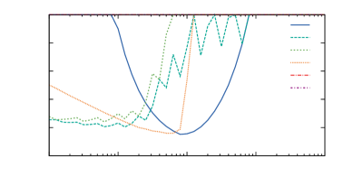
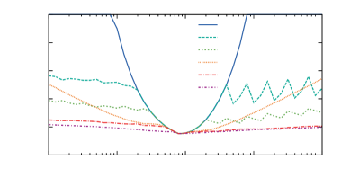
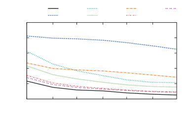
Comparisons of the different strategies over a wide range of $\lambda$ values and three different dictionary sizes are presented in Figs. 5–7. The mean number of iterations for all $\rho$ values is plotted against $\lambda$, and also compared with the minimum number of iterations obtained for the best fixed choice of $\rho$. The most important observations to be made are:

• The standard residuals give similar performance to the normalised residuals for the larger values of $\lambda$ since in this regime the normalisation quantities turn out to be close to unity.

• At smaller values of $\lambda$, the normalised residuals give much better performance.

• Considered over the entire range of $\lambda$ values, the normalised residuals all give better performance than their un-normalised counterparts.

• Of the methods using normalised residuals, the adaptive $\tau$ methods based on Eq. (54) gives substantially better performance than the standard methods.

VI-C Convolutional BPDN Problem

(a) Standard residuals

(b) Normalised residuals

Figure 8: Mean number of iterations (averaged over all values of $\rho^{(0)}$) required to reach a relative stopping tolerance of $\epsilon_{\mathrm{rel}}=10^{-3}$ for different variants of the adaptive $\rho$ policy, and for standard and normalised residuals, in a CBPDN problem with a $8\times 8\times 64$ dictionary and varying $\lambda$. The variant labels are “Fixed”, indicating that $\rho$ is fixed at $\rho^{(0)}$ and is not adapted, of the form $\mu/\tau$, or of the form $\mu$/Auto, which indicates that $\tau$ is adapted as in Eq. (54), with $\tau_{\mathrm{max}}=100$ and $\xi=1$. “Fixed (min)” denotes the minimum number of iterations (i.e. not the mean) obtained via the best fixed choice of $\rho^{(0)}$ at each value of $\lambda$.

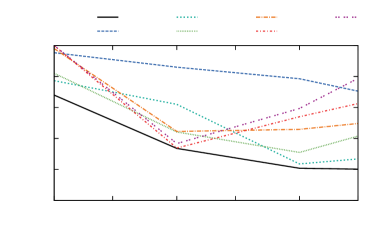
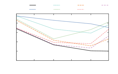
The penalty update strategies were also compared in application to a Convolutional BPDN problem consisting of jointly computing the representations of two $256\times 256$ pixel images (the well-known “Lena” and “Barbara” images), with a dictionary consisting of 64 filters of size $8\times 8$ samples and for a range of $\lambda$ and $\rho^{(0)}$ values. It can be seen from Fig. 8 that the normalised residuals give good performance for $\lambda\leq 0.1$, but for larger values of $\lambda$ neither standard nor normalised residuals provide performance close to that of the best fixed $\rho$.

Figure 9: Evolution of primal and dual residuals for two different choices of $\xi$ in a CBPDN problem with an $8\times 8\times 32$ dictionary, $\lambda=0.3$, and $\rho^{(0)}=251$. The $\rho$ update policy was as in Eq. (53), with normalised residuals, $\mu=1.2$, and with adaptive $\tau$ as in Eq. (54), with $\tau_{\mathrm{max}}=100$.

This is an indication that $\xi=1$ is not a suitable choice in this case, for which $\xi=5$ gives better performance, as illustrated in Fig. 9.

Figure 10: Mean number of iterations, averaged over all values of $\rho^{(0)}$, against $\lambda$ and $\xi$ for a CBPDN problem with an $8\times 8\times 64$ dictionary. The $\rho$ update policy was as in Eq. (53), with normalised residuals, $\mu=1.2$, and with adaptive $\tau$ as in Eq. (54), with $\tau_{\mathrm{max}}=1000$.

Figure 11: Standard deviation of number of iterations with respect to $\rho^{(0)}$ in Fig. 10. Note that the variation with respect to $\rho$ is small where the mean number of iterations is small. The standard deviation is zero for small $\lambda$ and large $\xi$ because the number of iterations is clipped to 500 by the maximum iteration limit in this region.

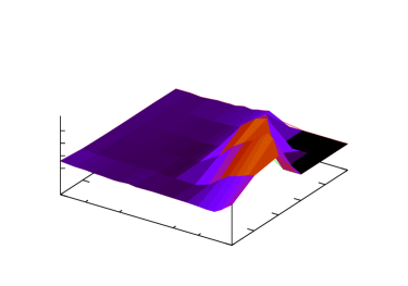
The effect of varying $\xi$ was investigated by running a large number of computational experiments for the CBPDN problem, with a $8\times 8\times 64$ dictionary and for different values of $\lambda$ (6 approximately logarithmically spaced values in the range $1\times 10^{-3}$ to $0.3$), $\rho$ (51 logarithmically spaced values in the range $10^{-1}\lambda$ to $10^{4}\lambda$), and $\xi$ (21 values in the range 0.3 to 10.0). The mean and standard deviation over $\rho^{(0)}$ of the number of iterations required to reach stopping tolerance $\epsilon_{\mathrm{abs}}=0,\epsilon_{\mathrm{rel}}=10^{-3}$ are displayed in Fig. 10 and 11 respectively. It can be observed that that the value of $\xi$ giving the minimum number of iterations varies with $\lambda$, and that considering the mean over $\rho^{(0)}$ of the number of iterations is a reasonable criterion since the variation with $\rho^{(0)}$ is small when $\xi$ is well chosen.

(a) Function fit to best values of $\xi$ for different $\lambda$.

(b) Mean iterations for different values of $\lambda$.

Figure 12: (a) shows the good fit of function $f(\lambda)=1+18.3^{\log_{10}(\lambda)+1}$ to the values of $\xi$ that minimise the mean (over all values of $\rho^{(0)}$) number of required iterations for different values of $\lambda$, determined by running a large number of simulations for different values of $\xi$, $\rho$, and $\lambda$. (b) shows the variation with $\lambda$ of the mean (over all values of $\rho^{(0)}$) number of iterations for the best choice of $\xi$ as in (a), for $\xi$ chosen according to the function $f(\lambda)$, and for three fixed choices of $\xi$. All simulations were for a CBPDN problem with a $8\times 8\times 64$ dictionary and $\epsilon_{\mathrm{abs}}=0,\epsilon_{\mathrm{rel}}=10^{-3}$. The $\rho$ update policy was as in Eq. (53), with normalised residuals, $\mu=1.2$, and with adaptive $\tau$ as in Eq. (54), with $\tau_{\mathrm{max}}=1000$.

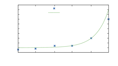
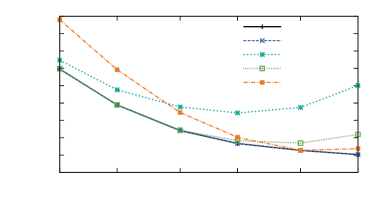
Since the best $\xi$ varies with $\lambda$, it is reasonable to ask, in the absence of any theory to guide the choice, whether there is a reliable way of making a good choice of $\xi$. By examining the data for the experiments used to generate Fig. 10 and 11, as well as for corresponding experiments with other dictionaries with 32, 96, and 128 filters of size $8\times 8$, it was determined that the function $f(\lambda)=1+a^{\log_{10}(\lambda)+1}$ with $a=18.3$ provides a reasonable fit to the best choice of $\xi$ for each $\lambda$, over all of these dictionaries. The fit of this function to the experimental data for the dictionary of 64 filters is shown in Fig. 12a, and a corresponding performance comparison in terms of mean iterations averaged over $\rho^{(0)}$ is displayed in Fig. 12b. Note that none of the fixed choices of $\xi$ provide good performance over the entire range of $\lambda$ values, while $\xi$ chosen according to $f(\lambda)$ gives the same performance as the best choices of $\xi$ at each $\lambda$.

Additional experiments using different test images (the “Kiel” and “Bridge” standard images) as well as different dictionary filters sizes ($12\times 12$) indicate that $f(\lambda)$ provides a good choice of $\xi$ over a wide range of conditions. While the choice of $a$ giving the best fit does vary with test images, filter size, and number of filters, the performance is not highly sensitive to the choice of $a$ (note that the mean iteration surface for large $\lambda$ is flat over a wide range of $\xi$ values in Fig. 10) and the choice of $a=18.3$ used in Fig. 12a was found to give performance at or close to the best choice of $\xi$ in all the cases considered.

VII Conclusion

The scaling properties of the standard definitions of the primal and dual residuals are shown to represent a potentially serious weakness in a popular adaptive penalty strategy [7] for ADMM algorithms. The proposed solution is to normalise these residuals so that they become invariant to scalings of the ADMM problem to which the solution is also invariant. The impact of this issue is demonstrated using BPDN sparse coding as an example problem. These experiments show that the standard adaptive penalty strategy [7] performs very poorly in certain cases, while the proposed modification based on normalised residuals is more robust.

There is, however, a more serious issue that is not so easily resolved: the unknown scaling relationship between the residuals and the solution distance from optimality implies that the correct residual ratio to target, $\xi$, is unknown, and not necessarily unity. In some cases it is possible to construct a heuristic estimate of this value, but it is yet to be demonstrated that such an approach offers any real benefit over directly estimating a suitable choice of a fixed $\rho$ parameter.

In the interests of reproducible research, software implementations of the main algorithms proposed here are made publicly available [22].

Appendix A Scaling of the Graph Form Problem

Many signal and image processing inverse problems can be expressed in terms of the graph form problem [23]

$$\operatorname*{arg\,min}_{\mathbf{x},\mathbf{z}}f(\mathbf{x})+g(\mathbf{z})\;\text{ such that }\;A\mathbf{x}=\mathbf{z}\;,$$ (65)

which is a special case of Eq. (8) with $B=-I$ and $\mathbf{c}=0$. In this case there is a slightly different set of scalings of the problem under which the solution is invariant, for which the most general scaled problem $\tilde{P}$ is

$$\operatorname*{arg\,min}_{\mathbf{x},{\mathbf{z}}}\alpha f(\gamma\mathbf{x})+\alpha g(\delta\mathbf{z})\;\text{ s.t. }\;A\gamma\mathbf{x}=\delta\mathbf{z}\;,$$ (66)

which can be expressed as graph form problem in standard form as

$$\operatorname*{arg\,min}_{\mathbf{x},{\mathbf{z}}}\tilde{f}(\mathbf{x})+\tilde{g}(\mathbf{z})\;\text{ such that }\;\tilde{A}\mathbf{x}=\mathbf{z}$$ (67)

with

$$\tilde{f}(\mathbf{x})=\alpha f(\gamma\mathbf{x})\quad\tilde{g}(\mathbf{z})=\alpha g(\delta\mathbf{z})\quad\tilde{A}=\delta^{-1}\gamma A\;.$$ (68)

The Lagrangian is

$$\tilde{L}({\mathbf{x}},{\mathbf{z}},{\mathbf{y}})=\alpha f(\gamma\mathbf{x}) +\alpha g(\delta\mathbf{z})+\mathbf{y}^{T}(\delta^{-1}\gamma A\mathbf{x}-\mathbf{z})\;,$$ (69)

and the primal and dual feasibility conditions are

$$\delta^{-1}\gamma A\tilde{\mathbf{x}}^{*}-\tilde{\mathbf{z}}^{*}=0\;,$$ (70)

and

$$0\in\partial\tilde{L}(\cdot,\tilde{\mathbf{z}}^{*},\tilde{\mathbf{y}}^{*})\;\Rightarrow\; 0\!\in\!\alpha\gamma[\partial f(\cdot)](\gamma\tilde{\mathbf{x}}^{*})+\delta^{-1}\gamma A^{T}\tilde{\mathbf{y}}^{*}=0$$ (71)

$$0\in\partial\tilde{L}(\tilde{\mathbf{x}}^{*},\cdot,\tilde{\mathbf{y}}^{*})\;\Rightarrow\; 0\!\in\!\alpha\delta[\partial g(\cdot)](\delta\tilde{\mathbf{z}}^{*})-\tilde{\mathbf{y}}^{*}=0$$ (72)

respectively. It is easily verified that if $\mathbf{x}^{*}$, $\mathbf{z}^{*}$, and $\mathbf{y}^{*}$ satisfy the optimality criteria Eq. (19), (20), and (21) for problem $P$, then

$$\tilde{\mathbf{x}}^{*}=\gamma^{-1}\mathbf{x}^{*}\quad\;\;\tilde{\mathbf{z}}^{*}=\delta^{-1}\mathbf{z}^{*}\quad\;\;\tilde{\mathbf{y}}^{*}=\alpha\delta\mathbf{y}^{*}$$ (73)

satisfy the primal and dual feasibility criteria for $\tilde{P}$.

The augmented Lagrangian for $\tilde{P}$ is

$$\tilde{L}_{\tilde{\rho}}(\mathbf{x},\mathbf{z},\mathbf{y}) =\alpha f(\gamma\mathbf{x})+\alpha g(\delta\mathbf{z})$$

$$+\alpha\left(\alpha^{-1}\delta^{-1}\mathbf{y}^{T}\right)(\gamma A\mathbf{x}-\delta\mathbf{z})$$

$$+\alpha\left(\alpha^{-1}\delta^{-2}\tilde{\rho}\right)\frac{1}{2}\left\|\gamma A\mathbf{x}-\delta\mathbf{z}\right\|_{2}^{2}\;,$$ (74)

so that setting

$$\tilde{\rho}=\alpha\delta^{2}\rho$$ (75)

gives

$$\tilde{L}_{\tilde{\rho}}(\mathbf{x},\mathbf{z},\mathbf{y})=\alpha L_{\rho}\left(\gamma\mathbf{x},\delta\mathbf{z},\alpha^{-1}\delta^{-1}\mathbf{y}\right)\;.$$ (76)

Appendix B BPDN Scaling Properties

The scaling properties of the BPDN problem with respect to the scalar multiplication of the input signal $\boldsymbol{\varsigma}$ depend on whether the dictionary is considered to have fixed scaling or scale with the signal. The former is the more common situation since the dictionary is usually normalised, but the latter situation does occur in an endogenous sparse representation [24], in which the signal is also used as the dictionary (with constraints on the sparse representation to avoid the trivial solution), usually without normalisation of the dictionary.

B-A Fixed Dictionary

First, define problem $\tilde{P}$ with signal $\boldsymbol{\varsigma}$ scaled by $\delta$

$$\operatorname*{arg\,min}_{\mathbf{x}}\frac{1}{2}\left\|D\mathbf{x}-\delta\boldsymbol{\varsigma}\right\|_{2}^{2}+\delta\lambda\left\|\mathbf{z}\right\|_{1}\text{ s.t. }\mathbf{x}=\mathbf{z}\;,$$ (77)

representing the most common case in which the columns of $D$ are normalised and $D$ does not scale with $\boldsymbol{\varsigma}$. The corresponding Lagrangian is

$$\tilde{L}(\mathbf{x},\mathbf{z},\mathbf{y}) =\frac{1}{2}\left\|D\mathbf{x}-\delta\boldsymbol{\varsigma}\right\|_{2}^{2}+\delta\lambda\left\|\mathbf{z}\right\|_{1}+\mathbf{y}^{T}(\mathbf{x}-\mathbf{z})$$

$$=\frac{1}{2}\left\|D\delta\delta^{-1}\mathbf{x}-\delta\boldsymbol{\varsigma}\right\|_{2}^{2}+\delta\lambda\left\|\delta\delta^{-1}\mathbf{z}\right\|_{1}$$

$$\hskip 95.00014pt+\mathbf{y}^{T}(\delta\delta^{-1}\mathbf{x}-\delta\delta^{-1}\mathbf{z})$$

$$=\delta^{2}L(\delta^{-1}\mathbf{x},\delta^{-1}\mathbf{z},\delta^{-1}\mathbf{y})\;.$$ (78)

Comparing with Eq. (40) it is clear that we need to set

$$\alpha=\delta^{2}\quad\gamma=\delta^{-1}\quad\beta=\delta$$ (79)

to use the ADMM scaling results of Sec. III. In this case the scaling behaviour is such that changing $\delta$ does not alter the ratio of primal and dual residuals. Note that this merely implies that the adaptive penalty parameter policy with standard residuals is not guaranteed to fail when the signal is scaled; it does not follow that the problem scaling is such that normalised residuals are not necessary.

B-B Dictionary Scales with Signal

In the second form of scaling, $D$ is not normalised, and scales linearly with $\boldsymbol{\varsigma}$. In this case problem $\tilde{P}$ with signal $\boldsymbol{\varsigma}$ and dictionary $D$ scaled by $\delta$ is

$$\operatorname*{arg\,min}_{\mathbf{x}}\frac{1}{2}\left\|\delta D\mathbf{x}-\delta\boldsymbol{\varsigma}\right\|_{2}^{2}+\delta^{2}\lambda\left\|\mathbf{z}\right\|_{1}\text{ s.t. }\mathbf{x}=\mathbf{z}\;.$$ (80)

The corresponding Lagrangian is

$$\tilde{L}(\mathbf{x},\mathbf{z},\mathbf{y}) =\frac{1}{2}\left\|\delta D\mathbf{x}-\delta\boldsymbol{\varsigma}\right\|_{2}^{2}+\delta^{2}\lambda\left\|\mathbf{z}\right\|_{1}+\mathbf{y}^{T}(\mathbf{x}-\mathbf{z})$$

$$=\frac{\delta^{2}}{2}\left\|D\mathbf{x}-\boldsymbol{\varsigma}\right\|_{2}^{2}+\delta^{2}\lambda\left\|\mathbf{z}\right\|_{1}$$

$$\hskip 73.00014pt+\delta^{2}\delta^{-2}\mathbf{y}^{T}(\mathbf{x}-\mathbf{z})$$

$$=\delta^{2}L(\mathbf{x},\mathbf{z},\delta^{-2}\mathbf{y})\;.$$ (81)

Comparing with Eq. (40) it is clear that we need to set

$$\alpha=\delta^{2}\quad\gamma=1\quad\beta=1$$ (82)

to use the ADMM scaling results of Sec. III. In this case the scaling behaviour is such that changing $\delta$ does alter the ratio of primal and dual residuals, and the adaptive penalty parameter policy with standard residuals is guaranteed to perform poorly for all but a restricted range of signal scaling values $\delta$.

Appendix C A Degenerate Case

An unusual degenerate case involving the TV-$\ell_{1}$ problem [25] illustrates that even the proposed normalised definitions of residuals cannot always be applied without analysis of the specific problem. This problem can be written as

$$\operatorname*{arg\,min}_{\mathbf{x}}\|\mathbf{x}-\mathbf{s}\|_{1}+\lambda\|\sqrt{(G_{0}\mathbf{x})^{2}+(G_{1}\mathbf{x})^{2}}\|_{1}\;,$$ (83)

which can be expressed in standard ADMM form Eq. (8) (see [26, Sec. 2.4.4]) with

$$\!\!\!f(\mathbf{x})=0\;\;\;\;\;g(\mathbf{z})=\|\mathbf{z}_{s}-\mathbf{s}\|_{1}+\lambda\|\sqrt{\mathbf{z}_{0}^{2}+\mathbf{z}_{1}^{2}}\|_{1}$$

$$A=\left(\begin{array}[]{c}G_{0}\\ G_{1}\\ I\end{array}\right)\;B=-I\;\;\;\mathbf{c}=\left(\begin{array}[]{c}0\\ 0\\ \mathbf{s}\end{array}\right)\;\mathbf{z}=\left(\begin{array}[]{c}\mathbf{z}_{0}\\ \mathbf{z}_{1}\\ \mathbf{z}_{s}\end{array}\right).$$ (93)

Since $f(\mathbf{x})=0$, dual feasibility condition Eq. (20) is simply $A^{T}\mathbf{y}^{*}=0$ and Eq. (24), from which the definition Eq. (25) is derived, degenerates to

$$\rho A^{T}B(\mathbf{z}^{(k+1)}-\mathbf{z}^{(k)})=A^{T}\mathbf{y}^{(k+1)}\;.$$ (94)

Clearly $A^{T}\mathbf{y}^{(k+1)}$ is unsuitable either as a normalisation term for the dual residual or as a factor in the stopping tolerance.

References

- [1] T. Goldstein and S. J. Osher, “The split Bregman method for l1-regularized problems,” SIAM Journal on Imaging Sciences, vol. 2, no. 2, pp. 323–343, 2009. doi:10.1137/080725891
- [2] S. Boyd, N. Parikh, E. Chu, B. Peleato, and J. Eckstein, “Distributed optimization and statistical learning via the alternating direction method of multipliers,” Foundations and Trends in Machine Learning, vol. 3, no. 1, pp. 1–122, 2010. doi:10.1561/2200000016
- [3] M. V. Afonso, J. M. Bioucas-Dias, and M. A. T. Figueiredo, “An Augmented Lagrangian approach to the constrained optimization formulation of imaging inverse problems,” IEEE Transactions on Image Processing, vol. 20, no. 3, pp. 681–695, Mar. 2011. doi:10.1109/tip.2010.2076294
- [4] E. Ghadimi, A. Teixeira, I. Shames, and M. Johansson, “Optimal parameter selection for the alternating direction method of multipliers (ADMM): Quadratic problems,” IEEE Transactions on Automatic Control, vol. 60, no. 3, pp. 644–658, Mar. 2015. doi:10.1109/TAC.2014.2354892
- [5] A. U. Raghunathan and S. Di Cairano, “Alternating direction method of multipliers for strictly convex quadratic programs: optimal parameter selection,” in American Control Conference (ACC), Jun. 2014, pp. 4324–4329. doi:10.1109/ACC.2014.6859093
- [6] ——, “ADMM for convex quadratic programs: Linear convergence and infeasibility detection,” arXiv, Tech. Rep. arXiv:1411.7288v2, 2015.
- [7] B.-S. He, H. Yang, and S.-L. Wang, “Alternating direction method with self-adaptive penalty parameters for monotone variational inequalities,” Journal of Optimization Theory and Applications, vol. 106, pp. 337–356, 2000. doi:10.1023/a:1004603514434
- [8] A. Hansson, Z. Liu, and L. Vandenberghe, “Subspace system identification via weighted nuclear norm optimization,” CoRR, vol. abs/1207.0023, 2012. [Online]. Available: http://arxiv.org/abs/1207.0023
- [9] Z. Liu, A. Hansson, and L. Vandenberghe, “Nuclear norm system identification with missing inputs and outputs,” Systems & Control Letters, vol. 62, no. 8, pp. 605 – 612, 2013. doi:10.1016/j.sysconle.2013.04.005
- [10] V. Q. Vu, J. Cho, J. Lei, and K. Rohe, “Fantope projection and selection: A near-optimal convex relaxation of sparse PCA,” in Advances in Neural Information Processing Systems 26, C. J. C. Burges, L. Bottou, M. Welling, Z. Ghahramani, and K. Q. Weinberger, Eds., 2013, pp. 2670–2678.
- [11] M.-D. Iordache, J. M. Bioucas-Dias, and A. Plaza, “Collaborative sparse regression for hyperspectral unmixing,” IEEE Transactions on Geoscience and Remote Sensing, vol. 52, no. 1, pp. 341–354, Jan. 2014. doi:10.1109/TGRS.2013.2240001
- [12] D. S. Weller, A. Pnueli, O. Radzyner, G. Divon, Y. C. Eldar, and J. A. Fessler, “Phase retrieval of sparse signals using optimization transfer and ADMM,” Proc. IEEE Intl. Conf. on Image Processing, pp. 1342–6, 2014.
- [13] B. Wohlberg, “Efficient convolutional sparse coding,” in Proceedings of IEEE International Conference on Acoustics, Speech, and Signal Processing (ICASSP), Florence, Italy, May 2014, pp. 7173–7177. doi:10.1109/ICASSP.2014.6854992
- [14] J.-B. Hiriart-Urruty and C. Lemaréchal, Fundamentals of Convex Analysis. Springer, 2004.
- [15] J. Eckstein, “Augmented Lagrangian and alternating direction methods for convex optimization: A tutorial and some illustrative computational results,” Rutgers Center for Operations Research, Rutgers University, Rutcor Research Report RRR 32-2012, December 2012. [Online]. Available: http://rutcor.rutgers.edu/pub/rrr/reports2012/32_2012.pdf
- [16] S.-L. Wang and L. Z. Liao, “Decomposition method with a variable parameter for a class of monotone variational inequality problems,” Journal of Optimization Theory and Applications, vol. 109, pp. 415–429, 2001. doi:10.1023/a:1017522623963
- [17] H. D. Mittelmann, “An independent benchmarking of SDP and SOCP solvers,” Mathematical Programming, vol. 95, no. 2, pp. 407–430, 2003. doi:10.1007/s10107-002-0355-5
- [18] A. Wächter and L. T. Biegler, “On the implementation of an interior-point filter line-search algorithm for large-scale nonlinear programming,” Mathematical Programming, vol. 106, no. 1, pp. 25–57, 2006. doi:10.1007/s10107-004-0559-y
- [19] A. Ramdas and R. J. Tibshirani, “Fast and flexible admm algorithms for trend filtering,” Journal of Computational and Graphical Statistics, vol. 25, no. 3, pp. 839–858, 2016. doi:10.1080/10618600.2015.1054033
- [20] S. S. Chen, D. L. Donoho, and M. A. Saunders, “Atomic decomposition by basis pursuit,” SIAM J. Sci. Comput., vol. 20, no. 1, pp. 33–61, 1998. doi:10.1137/S1064827596304010
- [21] B. Wohlberg, “Efficient algorithms for convolutional sparse representations,” IEEE Transactions on Image Processing, vol. 25, no. 1, pp. 301–315, Jan. 2016. doi:10.1109/TIP.2015.2495260
- [22] ——, “SParse Optimization Research COde (SPORCO),” Software library available from http://purl.org/brendt/software/sporco, 2016.
- [23] N. Parikh and S. Boyd, “Block splitting for distributed optimization,” Mathematical Programming Computation, vol. 6, no. 1, pp. 77–102, 2014. doi:10.1007/s12532-013-0061-8
- [24] E. L. Dyer, A. C. Sankaranarayanan, and R. G. Baraniuk, “Greedy feature selection for subspace clustering,” Journal of Machine Learning Research, vol. 14, pp. 2487–2517, 2013. [Online]. Available: http://jmlr.org/papers/v14/dyer13a.html
- [25] S. Alliney, “Digital filters as absolute norm regularizers,” IEEE Transactions on Signal Processing, vol. 40, no. 6, pp. 1548–1562, Jun. 1992. doi:10.1109/78.139258
- [26] E. Esser, “Primal dual algorithms for convex models and applications to image restoration, registration and nonlocal inpainting,” Ph.D. dissertation, University of California, Los Angeles, 2010.