A Model Order Reduction Algorithm for Estimating the Absorption Spectrum

Abstract

The ab initio description of the spectral interior of the absorption spectrum poses both a theoretical and computational challenge for modern electronic structure theory. Due to the often spectrally dense character of this domain in the quantum propagator’s eigenspectrum for medium-to-large sized systems, traditional approaches based on the partial diagonalization of the propagator often encounter oscillatory and stagnating convergence. Electronic structure methods which solve the molecular response problem through the solution of spectrally shifted linear systems, such as the complex polarization propagator, offer an alternative approach which is agnostic to the underlying spectral density or domain location. This generality comes at a seemingly high computational cost associated with solving a large linear system for each spectral shift in some discretization of the spectral domain of interest. In this work, we present a novel, adaptive solution to this high computational overhead based on model order reduction techniques via interpolation. Model order reduction reduces the computational complexity of mathematical models and is ubiquitous in the simulation of dynamical systems and control theory. The efficiency and effectiveness of the proposed algorithm in the ab initio prediction of X-Ray absorption spectra is demonstrated using a test set of challenging water clusters which are spectrally dense in the neighborhood of the oxygen $K$-edge. Based on a single, user defined tolerance we automatically determine the order of the reduced models and approximate the absorption spectrum up to the given tolerance. We also illustrate that, for the systems studied, the automatically determined model order increases logarithmically with the problem dimension, compared to a linear increase of the number of eigenvalues within the energy window. Furthermore, we observed that the computational cost of the proposed algorithm only scales quadratically with respect to the problem dimension.

1 Introduction

With recent advances in laser light source technology, X-ray absorption spectroscopy (XAS) has become an important probative tool in chemical physics.¹ The ability of XAS to simultaneously characterize both the electronic and geometrical structure of chemical systems has made it indispensable in the fields of catalysis and photophysics.^{2, 3, 4, 5, 6} However, despite the capability of XAS to obtain a wealth of chemically relevant information, the complexity of experimentally obtained XAS spectra often requires a theoretical supplement to obtain a meaningful interpretation of the query phenomenon.^{7, 8} Thus, the ability to properly describe the high-energy electronic excitations of molecular systems theoretically is critical in modern electronic structure theory.

In light of its importance in physical chemistry, the prediction of XAS properties poses an interesting challenge for traditional electronic structure methods. This challenge is rooted in the fact that the X-Ray region is buried deep within the eigenspectrum of the Hamiltonian and is often spectrally dense. For example, in near edge X-Ray absorption fine structure (NEXAFS) spectroscopy, the spectrum consists of many excited states that correspond to excitations of core electrons to diffuse quasi bound levels. Thus, as system sizes increase, the number of states in the given energy region increases dramatically. Further, it is important to note that, because very large basis sets are often required to properly describe the rather diffuse nature of these excited states, the increase in complexity leads to poor scaling with system size.

Many electronic structure methods have been extended to the description of high-energy, X-ray electronic excitations in recent years. In the time domain, real-time density functional theory^{9, 10, 11} has been shown to excellently reproduce the X-ray K-edge for molecules within relatively short simulation times.^{12, 13} For large systems, however, time-domain methods have difficulty taking full advantage of concurrency on modern computing architectures, and are thus not yet a sustainable avenue in routine theoretical inquiry of these phenomena. In contrast, frequency domain approaches are often favored in these types of calculations as they may be cast as computationally scalable linear algebra problems which are well suited for massive concurrency. Frequency domain approaches to treat electronic excitations may be separated into two categories which obtain equivalent information: methods which aim to obtain a spectral decomposition of the quantum propagator, i.e., eigenproblem based methods, and methods which solve the response problem directly through the solution of linear systems of equations.

Recasting electronic structure methods into eigenproblems has long been the de facto standard frequency domain method for electronically excited states. Through knowledge of the poles (eigenroots) of the quantum propagator, one has direct access to information regarding the electronic excitations (resonances) of the molecular system. In addition, such a spectral decomposition may be used to treat off-resonant perturbations through interpolation schemes known as sum-over-states expressions¹⁴. Much work has gone into the development of these methods in both wave function theory, such as those based on the coupled-cluster (CC)^{15, 16, 17, 18, 19} and algebraic diagrammatic construction (ADC)^{20, 21} expansions of the many-body wave function, and self-consistent field theory, such as the linear response time-dependent Hartree–Fock (TD-HF)^{22, 23, 24, 25} and density functional theory (TD-DFT)^{26, 27}. These methods have been shown to accurately predict and reproduce both low-^{28, 29} and high-energy^{30, 31, 32, 33, 34, 35, 12} electronic excitations in molecular systems. Despite their accuracy, however, eigenproblem based methods possess an inherent challenge in the description of high-energy excited states when the eigenroots of interest are buried deep in the eigenspectrum. Traditional methods used to partially diagonalize the propagator, such as the block-Davidson method^{36, 37, 38}, are designed to converge to the extreme ends of the eigenspectrum with no built-in mechanism to establish the spectrum’s interior. Several approaches have been described to overcome this problem ³⁹, including energy specific^{30, 32} and restricted energy window methods^{33, 34, 35} when the eigenroots of interest are well-separated. Further, in spectrally dense regions of the propagator’s eigenspectrum, iterative diagonalization algorithms require the resolution of many more roots than is often practical to ensure smooth convergence.

Methods which solve the response problem through the solutions of linear systems offer an attractive alternative to eigenproblem based approaches in the description of high-energy excitations because they have an intrinsic mechanism to probe the interior of the energy spectrum. In these methods, the probing frequency of the applied perturbation is a chosen parameter.^{22, 28} Thus, the interior of the spectrum is easily probed through a number of solutions of linear system of equations in the desired frequency domain. This simplicity does, however, come at a seemly significant computational cost compared to eigenproblem based methods. While eigenproblems are able to directly obtain many poles of the eigenspectrum simultaneously, one must solve the linear problem many times over some discretization of the frequency domain to obtain similar results. In general, this discretization must be quite dense to achieve a reasonable accuracy and thus can be more expensive than their eigenproblem based counterparts. Approaches using linear systems and based on the complex polarization propagator (CPP), such as CPP-CC^{40, 41, 42} and CPP-SCF,^{43, 28, 14, 44} have been shown to be successful in the description of both high^{45, 46, 47, 48, 49} and low⁵⁰ energy properties of molecular systems and have been extended to relativistic Hamiltonians as well⁵¹.

In this work, we introduce a general framework for the prediction of spectrally interior molecular response properties based on model order reduction (MOR) via interpolation. MOR techniques have been successfully applied in different fields of computation science and engineering, where it reduces the computational complexity of mathematical models in numerical simulations. Examples include structural dynamics, sound and vibration analysis, and control theory ⁵². The MOR algorithm proposed in this paper aims to overcome the large computational overhead associated with the spectral discretization required by linear system based methods while maintaining the accuracy associated with eigenproblem based methods. Further, the proposed algorithm will be shown to allow for the massively scalable parallelism that is well suited for modern computing architectures.

2 Linear response and absorption spectrum

In the semi-classical theory of molecular light-matter interaction within the electric dipole approximation, the isotropic absorption cross section for the interaction with plane-polarized light, $\sigma(\omega)$, at a particular perturbing frequency, $\omega$, is proportional to the trace of the dynamic polarizability tensor, $\boldsymbol{\alpha}(\omega)$,

$$\sigma(\omega)\propto\omega\operatorname{Im}\left(\operatorname{Tr}\left[\boldsymbol{\alpha}(\widetilde{\omega})\right]\right),\qquad\widetilde{\omega}=\omega+i\eta,$$ (1)

where $\eta>0$ is a small damping parameter to ensure the convergence of $\boldsymbol{\alpha}$ in the spectral neighborhoods of resonant perturbations. Within the linear response regime of the first-order polarization propagator approximation (FOPPA)¹⁴, the dynamic polarizability tensor may be written as

$$\boldsymbol{\alpha}(\widetilde{\omega})=\mathbf{d}^{\top}\mathbf{G}^{-1}(\widetilde{\omega})\mathbf{d},\qquad\mathbf{d}=\begin{bmatrix}\mathbf{d}_{x}&\mathbf{d}_{y}&\mathbf{d}_{z}\\ \mathbf{d}_{x}&\mathbf{d}_{y}&\mathbf{d}_{z}\end{bmatrix}.$$ (2)

Here, $\{\mathbf{d}_{i}\text{ }|\text{ }i\in\{x,y,z\}\}$ is the set of dipole operators expressed in the molecular orbital (MO) basis, and $\mathbf{G}(\widetilde{\omega})$ is the first-order polarization propagator. In the following algorithm developments, we restrict the discussion to the FOPPA using a Hartree–Fock reference (TD-HF), although the algorithm presented is completely general to any choice of propagator or reference. Within TD-HF, $\mathbf{G}(\widetilde{\omega})$ may be written as

$$\mathbf{G}(\widetilde{\omega})=\mathbf{H}-\widetilde{\omega}\mathbf{S},$$ (3)

where

$$\mathbf{H}=\begin{bmatrix}\mathbf{A}&\mathbf{B}\\ \mathbf{B}&\mathbf{A}\end{bmatrix},\qquad\mathbf{S}=\begin{bmatrix}[r]\mathbf{I}&\mathbf{0}\\ \mathbf{0}&-\mathbf{I}\end{bmatrix},$$ (4)

with $\mathbf{S}=\mathbf{S}^{\top}=\mathbf{S}^{-1}$ and

$$A_{ai,bj} =\delta_{ij}\delta_{ab}\left(\epsilon_{a}-\epsilon_{i}\right)+(ai||bj),$$ (5)

$$B_{ai,bj} =(ab||ij).$$ (6)

Here, we have adopted the convention of denoting occupied MOs with indices $i,j,k,\ldots$ and virtual (unoccupied) MOs with indices $a,b,c,\ldots$ $\{\epsilon_{p}\}$ is taken to be the set of canonical Hartree–Fock MO eigenenergies and the moieties $(\cdot||\cdot)$ are the MO basis representation of the anti-symmetrized electron-repulsion integrals in Mulliken notation. In this work, we restrict our treatment to the use of strictly real MOs to allow for further simplification of the working expressions.

In order to study the spectrum of the pencil $(\mathbf{H},\mathbf{S})$ let

$$\mathbf{\Omega}=\mathbf{S}^{-1}\mathbf{H}=\begin{bmatrix}[r]\mathbf{A}&\mathbf{B}\\ -\mathbf{B}&-\mathbf{A}\end{bmatrix}.$$ (7)

Although the matrix $\mathbf{\Omega}$ is non-symmetric, it has a number of special properties ^{15, 53, 54}. If $\mathbf{H}$ is positive definite, it may be shown that $\mathbf{\Omega}$ possesses a structured eigendecomposition ^{24, 55}, i.e.,

$$\begin{bmatrix}[r]\mathbf{A}&\mathbf{B}\\ -\mathbf{B}&-\mathbf{A}\end{bmatrix}=\begin{bmatrix}[r]\mathbf{U}&\mathbf{V}\\ \mathbf{V}&\mathbf{U}\end{bmatrix}\begin{bmatrix}[r]\mathbf{\Lambda}&\mathbf{0}\\ \mathbf{0}&-\mathbf{\Lambda}\end{bmatrix}\begin{bmatrix}[r]\mathbf{U}&-\mathbf{V}\\ -\mathbf{V}&\mathbf{U}\end{bmatrix}^{\top}$$ (8)

where $\mathbf{\Lambda}=\operatorname{diag}(\lambda_{1},\dotsc,\lambda_{n})$ consists of strictly positive eigenvalues, and the eigenvectors are normalized with respect to the metric $\mathbf{S}$,

$$\begin{bmatrix}[r]\mathbf{U}&-\mathbf{V}\\ -\mathbf{V}&\mathbf{U}\end{bmatrix}^{\top}\begin{bmatrix}[r]\mathbf{U}&\mathbf{V}\\ \mathbf{V}&\mathbf{U}\end{bmatrix}=\mathbf{I}.$$ (9)

As $\mathbf{H}$ is taken to be real in this work, it possesses additional properties that may be exploited in the development of efficient algorithms for estimating the absorption spectrum of the target system. In particular, we may apply the following similarity transformation

$$\mathbf{T}=\frac{1}{\sqrt{2}}\begin{bmatrix}[r]\mathbf{I}&\mathbf{I}\\ -\mathbf{I}&\mathbf{I}\end{bmatrix},\qquad\mathbf{T}^{-1}=\mathbf{T}^{\top},$$ (10)

to $\mathbf{G}(\widetilde{\omega})$, yielding

$$\mathbf{T}^{\top}\mathbf{G}(\widetilde{\omega})\mathbf{T}=\begin{bmatrix}\mathbf{K}&\mathbf{0}\\ \mathbf{0}&\mathbf{M}\end{bmatrix}-\widetilde{\omega}\begin{bmatrix}\mathbf{0}&\mathbf{I}\\ \mathbf{I}&\mathbf{0}\end{bmatrix},$$ (11)

where

$$\mathbf{M} \equiv\mathbf{A}+\mathbf{B},$$ (12)

$$\mathbf{K} \equiv\mathbf{A}-\mathbf{B},$$ (13)

which are, in most cases, positive definite. In this case, the polarizability tensor may be reformulated as

$$\boldsymbol{\alpha}(\widetilde{\omega})=\widetilde{\mathbf{d}}^{\top}\widetilde{\mathbf{G}}^{-1}(\widetilde{\omega})\widetilde{\mathbf{d}},\qquad\widetilde{\mathbf{d}}=\begin{bmatrix}\mathbf{d}_{x}&\mathbf{d}_{y}&\mathbf{d}_{z}\end{bmatrix},$$ (14)

where

$$\widetilde{\mathbf{G}}(\widetilde{\omega})=\mathbf{M}\mathbf{K}-\widetilde{\omega}^{2}\mathbf{I}.$$ (15)

Note that the dimension of $\widetilde{\mathbf{G}}(\widetilde{\omega})$ is only half the dimension of $\mathbf{G}(\widetilde{\omega})$. Furthermore, it can be shown that

$$\mathbf{M} =(\mathbf{X}-\mathbf{Y})\mathbf{\Lambda}(\mathbf{X}-\mathbf{Y})^{\top},$$ (16)

$$\mathbf{K} =(\mathbf{X}+\mathbf{Y})\mathbf{\Lambda}(\mathbf{X}+\mathbf{Y})^{\top},$$ (17)

and

$$(\mathbf{X}-\mathbf{Y})^{\top}(\mathbf{X}+\mathbf{Y})=\mathbf{I},$$ (18)

such that the eigenvalues $\pm\mathbf{\Lambda}$ may be computed by

$$\mathbf{M}\mathbf{K}=(\mathbf{X}-\mathbf{Y})\mathbf{\Lambda}^{2}(\mathbf{X}+\mathbf{Y})^{\top}.$$ (19)

Remark that by making use of $\mathbf{M}\mathbf{K}$, the dimension of the eigenvalue problem is also reduced by a factor of 2.^{56, 57}

3 Model order reduction of linear dynamical systems

In this section, we briefly review the theory of model order reduction for linear dynamical systems. The next section will examine its connection to the computation of the absorption spectrum within the FOPPA.

3.1 Linear dynamical systems

We consider the linear multiple-input multiple-output (MIMO) system

$$\mathbf{\Sigma}=\left\{\begin{aligned} \left(\mathbf{H}-s\mathbf{S}\right)\mathbf{x}(s)&=\mathbf{b}\,u(s)\\ \mathbf{y}(s)&=\mathbf{c}^{\top}\mathbf{x}(s)\end{aligned}\right.,$$ (20)

where $s$ is a derivative or shift operator, $\mathbf{H}\in\mathbb{R}^{n\times n}$ and $\mathbf{S}\in\mathbb{R}^{n\times n}$ are the system matrices, $\mathbf{b}\in\mathbb{R}^{n\times m}$, and $\mathbf{c}\in\mathbb{R}^{n\times p}$. We call $n$ the dimension (order) of the system $\mathbf{\Sigma}$, $\mathbf{x}\in\mathbb{R}^{n\times m}$ the state vector, $u\in\mathbb{R}$ the input, and $\mathbf{y}\in\mathbb{R}^{p\times m}$ the output ⁵². Note that the system $\mathbf{\Sigma}$ is completely characterized by the quadruple $(\mathbf{H},\mathbf{S},\mathbf{b},\mathbf{c})$.

The transfer function, $\boldsymbol{\gamma}(s)$, of $\mathbf{\Sigma}$ is defined as

$$\boldsymbol{\gamma}(s)=\mathbf{c}^{\top}\left(\mathbf{H}-s\mathbf{S}\right)^{-1}\mathbf{b},$$ (21)

and describes the relation between the input and output of $\mathbf{\Sigma}$, i.e., $\mathbf{y}(s)=\boldsymbol{\gamma}(s)u(s)$. For the remainder, we will assume that $n\gg 1$, $m\ll n$, $p\ll n$, and $u(s)\equiv 1$ for all $s$.

3.2 State space transformation

In some cases, it might be more advantageous to describe the system from a different point of view as the original one. In these cases, we may perform a non-singular state transformation $\mathbf{T}$, i.e., $\det(\mathbf{T})\neq 0$, yielding the transformed state

$$\widetilde{\mathbf{x}}=\mathbf{T}^{-1}\mathbf{x},$$ (22)

of the transformed system

$$\widetilde{\mathbf{\Sigma}}=\left\{\begin{aligned} \left(\widetilde{\mathbf{H}}-s\widetilde{\mathbf{S}}\right)\widetilde{\mathbf{x}}(s)&=\widetilde{\mathbf{b}}\,u(s)\\ \mathbf{y}(s)&=\widetilde{\mathbf{c}}^{\top}\widetilde{\mathbf{x}}(s)\end{aligned}\right.,$$ (23)

where $\widetilde{\mathbf{H}}=\mathbf{T}^{-1}\mathbf{H}\mathbf{T}$, $\widetilde{\mathbf{S}}=\mathbf{T}^{-1}\mathbf{S}\mathbf{T}$, $\widetilde{\mathbf{b}}=\mathbf{T}^{-1}\mathbf{b}$, and $\widetilde{\mathbf{c}}^{\top}=\mathbf{c}^{\top}\mathbf{T}$. Remark that $\mathbf{\Sigma}$ and $\widetilde{\mathbf{\Sigma}}$ admit the same transfer function as well as the same output. Therefore, we call the systems $\mathbf{\Sigma}$ and $\widetilde{\mathbf{\Sigma}}$ equivalent.

3.3 Reduced order models

The evaluation of the transfer function of a system $\mathbf{\Sigma}$ requires a linear system solve for every value of $s$. In cases where the system dimension $n$ is large and a high resolution is required, i.e., a high number of values of $s$, the evaluation of the transfer function is very expensive. In this work, we examine the effectiveness of model order reduction (MOR) techniques to circumvent this expense. MOR for linear dynamical systems is a technique that approximates a system $\mathbf{\Sigma}$ by another system $\widehat{\mathbf{\Sigma}}$ of the same form but of a much lower dimension (order) $k\ll n$. Consequently, evaluating the transfer function of $\widehat{\mathbf{\Sigma}}$ is relatively inexpensive as it only involves linear system solves of dimension $k$ instead of linear system solves of dimension $n$ for $\mathbf{\Sigma}$.

Let the system $\mathbf{\Sigma}$ be given by 20 and define a non-singular matrix $\mathbf{V}\in\mathbb{R}^{n\times k}$ with orthonormal columns, i.e., $\mathbf{V}^{\top}\mathbf{V}=\mathbf{I}$. Then, a reduced order model $\widehat{\mathbf{\Sigma}}$ can be constructed by applying a Galerkin projection $\mathbf{P}=\mathbf{V}\mathbf{V}^{\top}$ onto $\mathbf{\Sigma}$, yielding

$$\widehat{\mathbf{\Sigma}}=\left\{\begin{aligned} \left(\widehat{\mathbf{H}}-s\widehat{\mathbf{S}}\right)\widehat{\mathbf{x}}(s)&=\widehat{\mathbf{b}}\,u(s)\\ \widehat{\mathbf{y}}(s)&=\widehat{\mathbf{c}}^{\top}\widehat{\mathbf{x}}(s)\end{aligned}\right.,$$ (24)

where $\widehat{\mathbf{H}}=\mathbf{V}^{\top}\mathbf{H}\mathbf{V}$, $\widehat{\mathbf{S}}=\mathbf{V}^{\top}\mathbf{S}\mathbf{V}$, $\widehat{\mathbf{b}}=\mathbf{V}^{\top}\mathbf{b}$, and $\widehat{\mathbf{c}}^{\top}=\mathbf{c}^{\top}\mathbf{V}$. Note that the length of the state vector $\widehat{\mathbf{x}}$ and the dimension of $\widehat{\mathbf{\Sigma}}$ are only $k\ll n$. The purpose of MOR is to construct a $\mathbf{V}$ such that the transfer function of $\widehat{\mathbf{\Sigma}}$ approximates very well the one of $\mathbf{\Sigma}$,

$$\boldsymbol{\gamma}_{\mathbf{\Sigma}}(s)\approx\boldsymbol{\gamma}_{\widehat{\mathbf{\Sigma}}}(s),$$ (25)

for all query $s$.

3.4 Model order reduction via moment matching

One way to construct a matrix $\mathbf{V}$ such that 25 holds is by examining the concepts of moments and moment matching⁵². Let the transfer function $\boldsymbol{\gamma}$ of $\mathbf{\Sigma}$ be given by 21. Then the $\ell$th moment of $\boldsymbol{\gamma}$ around the point $s=s_{\star}$ is defined as the $\ell$th derivative of $\boldsymbol{\gamma}$ evaluated at $s_{\star}$, i.e.,

$$\mathbf{m}_{\ell}(s_{\star}):=(-1)^{\ell}\left.\frac{d^{\ell}}{ds^{\ell}}\boldsymbol{\gamma}(s)\right|_{s=s_{\star}},$$ (26)

for $\ell\geq 0$. Consequently, since $\boldsymbol{\gamma}(s)=\mathbf{c}^{\top}\left(\mathbf{H}-s\mathbf{S}\right)^{-1}\mathbf{b}$, the moments at $s_{\star}$ are

$$\mathbf{m}_{\ell}(s_{\star})=\mathbf{c}^{\top}\left(\mathbf{H}-s_{\star}\mathbf{S}\right)^{-(\ell+1)}\mathbf{b},\qquad\ell>0.$$

Note also that the moments determine the coefficients of the Taylor series expansion of the transfer function $\boldsymbol{\gamma}$ in the neighborhood of $s_{\star}$

$$\boldsymbol{\gamma}(s)=\mathbf{m}_{0}(s_{\star})+\mathbf{m}_{1}(s_{\star})\frac{s-s_{\star}}{1!}+\mathbf{m}_{2}(s_{\star})\frac{(s-s_{\star})^{2}}{2!}+\cdots$$ (27)

Model order reduction via moment matching consists of constructing a subspace $\mathbf{V}\in\mathbb{R}^{n\times km}$ such that the original and reduced order model match moments

$$\mathbf{m}_{i_{j}}(s_{j})=\widehat{\mathbf{m}}_{i_{j}}(s_{j}),\qquad j=1,\ldots,k.$$ (28)

If all moments to be matched are chosen at zero, i.e., $s_{j}=0$ for $j=1,2,\ldots,k$, the corresponding model is known as a Padé approximation. In the general case, the problem 28 is known as rational interpolation and can be solved by choosing the projection matrix $\mathbf{V}$ such that

$$\mathbf{V}=\operatorname{span}\Big{[}\left(\mathbf{H}-s_{1}\mathbf{S}\right)^{-1}\mathbf{b}\quad\left(\mathbf{H}-s_{2}\mathbf{S}\right)^{-1}\mathbf{b}\quad\cdots\quad\left(\mathbf{H}-s_{k}\mathbf{S}\right)^{-1}\mathbf{b}\Big{]}.$$ (29)

It can be shown that the matrix $\mathbf{V}$ defined in 29 spans a rational Krylov subspace and matches all the $0$th moments at $s_{j}$. For more information about the connections between moment matching and rational interpolation, we refer the interested reader to Section 11 of Antoulas’ model order reduction book ⁵².

4 Estimating absorption spectrum without explicitly computing eigenvalues and eigenvectors

The most straightforward way to evaluate the absorption spectrum is to compute eigenvalues and the corresponding eigenvectors of $(\mathbf{H},\mathbf{S})$. However, as we indicated earlier, when the dimension of $\mathbf{H}$ and $\mathbf{S}$ becomes large (spectrally dense), this approach can be prohibitively expensive (complicated).

It has been shown⁵⁸ that a special $\mathbf{K}$-inner product Lanczos algorithm can be used to provide a good approximation to the overall structure of the absorption spectrum without explicitly computing the eigenvalues and eigenvectors of $(\mathbf{H},\mathbf{S})$. In particular, the Lanczos algorithm can reveal major absorption peaks in the low frequency region of the spectrum without too many iterations. However, the algorithm gives limited resolution of the absorption spectrum in the spectral interior as the Krylov subspace constructed by the Lanczos iteration contains little spectral information associated with interior eigenvalues of $(\mathbf{H},\mathbf{S})$.

We now propose an alternative way to evaluate the absorption spectrum without explicitly computing the eigenvalues and eigenvectors of $(\mathbf{H},\mathbf{S})$. This scheme focuses on approximating the dynamic polarizability tensor $\boldsymbol{\alpha}(\widetilde{\omega})$ defined in 2 and the absorption spectrum $\sigma(\omega)$ defined in 1 within a specific energy window directly.

Firstly, observe that the dynamic polarizability tensor 2 may be viewed simply as the expectation value of the inverse of $\mathbf{H}-\widetilde{\omega}\mathbf{S}$. Hence, the evaluation of $\boldsymbol{\alpha}(\widetilde{\omega})$ may be recast into a problem of solving linear equations, i.e., for a specific frequency $\omega$, we can directly evaluate the absorption spectrum 1 as follows

$$\sigma(\omega)\propto\omega\operatorname{Im}\left(\operatorname{Tr}\left[\mathbf{d}^{\top}\mathbf{x}(\widetilde{\omega})\right]\right),$$ (30)

where $\mathbf{x}$ is the solution of the linear system

$$\left(\mathbf{H}-\widetilde{\omega}\mathbf{S}\right)\mathbf{x}(\widetilde{\omega})=\mathbf{d}.$$ (31)

Secondly, the dynamic polarizability tensor 2 may also be viewed as the transfer function, i.e., the relation between input and output, of the linear dynamical system (see section 3.1)

$$\left\{\begin{aligned} \left(\mathbf{H}-\widetilde{\omega}\mathbf{S}\right)\mathbf{x}(\widetilde{\omega})&=\mathbf{d}\\ \mathbf{y}(\omega)&=\mathbf{d}^{\top}\mathbf{x}(\widetilde{\omega})\end{aligned}\right..$$ (32)

Consequently, the absorption spectrum can directly be obtained from the output variable $\mathbf{y}$

$$\sigma(\omega)\propto\omega\operatorname{Im}\left(\operatorname{Tr}\left[\mathbf{y}(\omega)\right]\right).$$ (33)

In order to evaluate the output $\mathbf{y}$ of system 32 for a given frequency, we again need to solve a linear system of the form 31.

Finally, by exploiting the block structure of $\mathbf{H}$ and performing a state space transformation with 10 (see section 3.2), we obtain an equivalent linear dynamical system for 32, but with a halved order,

$$\left\{\begin{aligned} \left(\mathbf{M}\mathbf{K}-\widetilde{\omega}^{2}\mathbf{I}\right)\widetilde{\mathbf{x}}(\widetilde{\omega})&=\widetilde{\mathbf{d}}\\ \mathbf{y}(\omega)&=2\,\widetilde{\mathbf{d}}^{\top}\mathbf{K}\,\widetilde{\mathbf{x}}(\widetilde{\omega})\end{aligned}\right.,$$ (34)

such that we obtain the following, compact expressions for the dynamic polarizability tensor

$$\boldsymbol{\alpha}(\widetilde{\omega})=2\,\widetilde{\mathbf{d}}^{\top}\mathbf{K}\left(\mathbf{M}\mathbf{K}-\widetilde{\omega}^{2}\mathbf{I}\right)^{-1}\widetilde{\mathbf{d}},$$ (35)

and the absorption spectrum

$$\sigma(\omega)\propto\omega\operatorname{Im}\left(\operatorname{Tr}\left[\widetilde{\mathbf{d}}^{\top}\mathbf{K}\left(\mathbf{M}\mathbf{K}-\widetilde{\omega}^{2}\mathbf{I}\right)^{-1}\widetilde{\mathbf{d}}\right]\right).$$ (36)

Note that the dimension of the linear systems to be solved in 36 is only half of the dimension of the linear system shown in 31.

Clearly, we cannot afford to evaluate $\sigma(\omega)$ for all $\omega$’s of interest. However, this connection to linear dynamical systems allows us to employ MOR techniques (see section 3.3) to reduce the number of $\sigma(\omega)$ evaluations in the full dimension. More precisely, we construct a function $\hat{\sigma}(\omega)$ that approximates $\sigma(\omega)$ within a specific energy window $[\omega_{\mathrm{min}},\omega_{\mathrm{max}}]$, but is much cheaper to evaluate. The construction of such an approximate function only requires solving a few linear systems of the form 31 or 34 at a few selected frequencies $\tau_{j}$, $j=1,2,\ldots,k$. The solutions of these linear systems are then used to construct a reduced order model which interpolates the full dynamic polarizability at $\tau_{j}$, and provides an approximation to the dynamic polarizability tensor 2 at other frequencies within the predefined energy window. When $k$ is small, both the construction and the evaluation of the reduced order model is significantly lower than other approaches that are either based on solving an eigenvalue problem or 31 at many different frequencies.

5 Interpolation based algorithms

Let the dimension of the matrix $\mathbf{H}$ defined in 4 be $2n\times 2n$. The dimension of the lower dimensional matrix $\widehat{\mathbf{H}}$ that we construct for the reduced order model is $3k\times 3k$, where $k\ll n$. One way to construct such a matrix is to first construct a subspace spanned by orthonormal columns of a matrix $\mathbf{V}\in\mathbb{R}^{2n\times 3k}$ and then project $\mathbf{H}$ onto such a subspace $\mathbf{V}$, i.e.,

$$\widehat{\mathbf{H}}=\mathbf{V}^{\top}\mathbf{H}\mathbf{V}.$$ (37)

If we also let $\widehat{\mathbf{S}}=\mathbf{V}^{\top}\mathbf{S}\mathbf{V}$ and $\widehat{\mathbf{d}}=\mathbf{V}^{\top}\mathbf{d}$, then the absorption spectrum can be approximated by

$$\widehat{\sigma}(\omega)\propto\omega\operatorname{Im}\left(\operatorname{Tr}\left[\widehat{\mathbf{d}}^{\top}\left(\widehat{\mathbf{H}}-\widetilde{\omega}\widehat{\mathbf{S}}\right)^{-1}\widehat{\mathbf{d}}\right]\right).$$ (38)

Clearly, the choice of the subspace $\mathbf{V}$ is crucial in maintaining the fidelity of the reduced order model. The subspace we use to construct the reduced order model takes the form

$$\mathbf{V}=\operatorname{span}\Big{[}\left(\mathbf{H}-\tau_{1}\mathbf{S}\right)^{-1}\mathbf{d}\quad\left(\mathbf{H}-\tau_{2}\mathbf{S}\right)^{-1}\mathbf{d}\quad\cdots\quad\left(\mathbf{H}-\tau_{k}\mathbf{S}\right)^{-1}\mathbf{d}\Big{]},$$ (39)

where $\tau_{j}$, $j=1,2,\ldots,k$, are the interpolation frequencies carefully chosen within the energy window of interest to ensure that

$$\sigma(\omega)\approx\widehat{\sigma}(\omega),$$ (40)

for all $\omega$ in the energy window of interest. It follows from the way $\mathbf{V}$ is constructed in 39 that $\widehat{\boldsymbol{\alpha}}$ interpolates $\boldsymbol{\alpha}$ at the interpolation frequencies, i.e.,

$$\boldsymbol{\alpha}(\tau_{j})=\widehat{\boldsymbol{\alpha}}(\tau_{j}),\qquad j=1,2,\ldots,k.$$ (41)

Furthermore, since the linear systems 32 and 34 have symmetric system matrices $(\mathbf{H},\mathbf{S})$ and $\mathbf{M}\mathbf{K}$, respectively, and the input and output matrices $\mathbf{b}$ and $\mathbf{c}$ are linearly dependent, the Galerkin projection becomes a Petrov–Galerkin projection⁵². Hence, the original systems 32 and 34 and its corresponding reduced order systems of dimension $k$ match $2k$ moments instead of only $k$ moments in the general case⁵². In order words, we can obtain the same accuracy for the reduced order models with fewer interpolation frequencies than the general (non-linearly dependent) case.

Algorithm 1 summarizes the construction of the reduced order model and how it is used to obtain an approximation of the absorption spectrum within an energy window of interest. Clearly, the higher the model order $k$, the more accurate the approximation. In the next section, we will show that even for a relatively small $k$, we can obtain a quite accurate approximation for $\sigma(\omega)$ in an interior spectral window that contains thousands of eigenvalues.

Input : Matrices $\mathbf{H},\mathbf{S},\mathbf{d}$,

Interpolation frequencies $\tau_{1},\tau_{2}\ldots,\tau_{k}$,

Frequencies $\omega_{1},\omega_{2},\ldots,\omega_{N}$, and $\eta$.

Output : Absorption spectrum $\widehat{\sigma}(\omega_{1}),\widehat{\sigma}(\omega_{2}),\ldots,\widehat{\sigma}(\omega_{N})$.

for $j=1,2,\ldots,k$ do

      1 Linear system solve $\mathbf{x}_{j}=\left(\mathbf{H}-\tau_{j}\mathbf{S}\right)^{-1}\mathbf{d}$.

end for

2QR factorization $\mathbf{X}=\mathbf{V}\mathbf{R}$.

3 Construct $\widehat{\mathbf{H}}=\mathbf{V}^{\top}\mathbf{H}\mathbf{V}$, $\widehat{\mathbf{S}}=\mathbf{V}^{\top}\mathbf{S}\mathbf{V}$, and $\widehat{\mathbf{d}}=\mathbf{V}^{\top}\mathbf{d}$.

for $j=1,2,\ldots,N$ do

      4 Compute $\widehat{\sigma}(\omega_{j})=\omega\operatorname{Im}\left(\operatorname{Tr}\left[\widehat{\mathbf{d}}^{\top}\left(\widehat{\mathbf{H}}-(\omega_{j}+i\eta)\widehat{\mathbf{S}}\right)^{-1}\widehat{\mathbf{d}}\right]\right)$.

end for

Algorithm 1 Absorption spectrum via model order reduction

Although algorithm 1 provides a general framework for constructing a reduced order model for estimating the absorption spectrum defined by $(\mathbf{H},\mathbf{S})$, it is more efficient to exploit the structure of $(\mathbf{H},\mathbf{S})$ and construct a reduced order model for 34 instead. Such a reduced order model may be obtained by projecting 34 onto a subspace defined by

$$\widetilde{\mathbf{V}}=\operatorname{span}\Big{[}\left(\mathbf{M}\mathbf{K}-\tau_{1}^{2}\mathbf{I}\right)^{-1}\widetilde{\mathbf{d}}\quad\left(\mathbf{M}\mathbf{K}-\tau_{2}^{2}\mathbf{I}\right)^{-1}\widetilde{\mathbf{d}}\quad\cdots\quad\left(\mathbf{M}\mathbf{K}-\tau_{k}^{2}\mathbf{I}\right)^{-1}\widetilde{\mathbf{d}}\Big{]},$$ (42)

where $\tau_{j}$, $j=1,2,\ldots,k$, are again the interpolation frequencies. Because the matrix $\mathbf{M}\mathbf{K}$ is self-adjoint with respect to the $\mathbf{K}$-inner product, it is more convenient to carry out the projection using the $\mathbf{K}$-inner product and projecting $\mathbf{M}\mathbf{K}$ onto a subspace spanned by a $\mathbf{K}$-orthonormal basis, i.e., $\widetilde{\mathbf{V}}^{\top}\mathbf{K}\widetilde{\mathbf{V}}=\mathbf{I}$ is satisfied. If we let

$$\widehat{\mathbf{M}\mathbf{K}} =\widetilde{\mathbf{V}}^{\top}\mathbf{K}\mathbf{M}\mathbf{K}\widetilde{\mathbf{V}},$$ (43)

$$\widehat{\mathbf{d}} =\widetilde{\mathbf{V}}^{\top}\mathbf{K}\widetilde{\mathbf{d}},$$ (44)

then the approximation to the absorption spectrum provided by the structure exploiting reduced order model can be expressed by

$$\widehat{\sigma}(\omega)\propto\omega\operatorname{Im}\left(\operatorname{Tr}\left[\widehat{\mathbf{d}}^{\top}\left(\widehat{\mathbf{M}\mathbf{K}}-\widetilde{\omega}^{2}\mathbf{I}\right)^{-1}\widehat{\mathbf{d}}\right]\right).$$ (45)

By exploiting the block structure of $\mathbf{H}$, we can prove that 38 and 45 are equivalent. However, the latter is cheaper to construct, both in terms of the number of floating point operations and memory usage, since it only involves matrices of size $n\times n$ and vectors of size $n$. The structure exploiting model order reduction algorithm for approximating the absorption spectrum is outlined in algorithm 2.

Input : Matrices $\mathbf{M},\mathbf{K},\widetilde{\mathbf{d}}$,

Interpolation frequencies $\tau_{1},\tau_{2}\ldots,\tau_{k}$,

Frequencies $\omega_{1},\omega_{2},\ldots,\omega_{N}$, and $\eta$.

Output : Absorption spectrum $\widehat{\sigma}(\omega_{1}),\widehat{\sigma}(\omega_{2}),\ldots,\widehat{\sigma}(\omega_{N})$.

for $j=1,2,\ldots,k$ do

      1 Linear system solve $\widetilde{\mathbf{x}}_{j}=\left(\mathbf{M}\mathbf{K}-\tau_{j}^{2}\mathbf{I}\right)^{-1}\widetilde{\mathbf{d}}$.

end for

2QR factorization $\widetilde{\mathbf{X}}=\widetilde{\mathbf{V}}\widetilde{\mathbf{R}}$, with $\widetilde{\mathbf{V}}^{\top}\mathbf{K}\widetilde{\mathbf{V}}=\mathbf{I}$.

3 Construct $\widehat{\mathbf{M}\mathbf{K}}=\widetilde{\mathbf{V}}^{\top}\mathbf{K}\mathbf{M}\mathbf{K}\widetilde{\mathbf{V}}$ and $\widehat{\mathbf{d}}=\widetilde{\mathbf{V}}^{\top}\mathbf{K}\widetilde{\mathbf{d}}$.

for $j=1,2,\ldots,N$ do

      4 Compute $\widehat{\sigma}(\omega_{j})=\omega\operatorname{Im}\left(\operatorname{Tr}\left[\widehat{\mathbf{d}}^{\top}\left(\widehat{\mathbf{M}\mathbf{K}}-(\omega_{j}+i\eta)^{2}\mathbf{I}\right)^{-1}\widehat{\mathbf{d}}\right]\right)$.

end for

Algorithm 2 Absorption spectrum via structure exploiting model order reduction

Note that both algorithms 1 and 2 require a choice of the interpolation frequencies $\tau_{j}$. The number of these interpolation frequencies and their locations solely determine the quality of the absorption spectrum approximations. The simplest way to choose these interpolation frequencies is to partition the energy window of interest evenly by a uniform interpolation grid. However, because the absorption spectrum can be highly oscillatory in certain regions within the energy window, a very fine grid may be needed to resolve the high oscillation. As a result, the order of the reduced order model, which is proportional to the number of interpolation frequencies, can be exceedingly high.

Figure 1: Adaptive refinement strategy for selecting the interpolation frequencies.

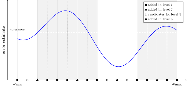
A more effective strategy for choosing the interpolation frequencies is to choose these frequencies in an adaptive fashion. We now propose a refinement strategy, which is graphically illustrated in fig. 1. To start this procedure, we choose in the first level a coarse, uniform grid of interpolation frequencies (marked by $\blacksquare$) to construct the level-1 reduced order model. The set of interpolation frequencies is refined by adding the midpoints (marked by $\blacktriangle$) between two adjacent level-1 interpolation frequencies. This enlarged set forms the second level of interpolation frequencies, yielding a more accurate level-2 reduced order model. Next, we choose the midpoints between two adjacent level-2 interpolation frequencies as candidates (marked by $\circ$) to enlarge the set in the third level. We also estimate the approximation error by computing the relative difference between the level-1 and level-2 reduced order models for the entire energy window. If the error estimate at an interval between two adjacent level-2 interpolation frequencies is above a prescribed error tolerance, the midpoint (marked by $\bullet$) is added to the existing set of interpolation frequencies. The enlarge set results in an even more accurate level-3 reduced order model. This refinement process continues until the error estimate at the entire energy window is below the threshold or when the refined model order exceeds an prescribed upper bound.

6 Computational results

The proposed automatic MOR algorithm has been implemented in the Chronus Quantum software package⁵⁹ and in MATLAB. The following numerical experiments were performed using a single Sandy–Bridge Intel Xeon compute node (E5-2650 v2 @ 2.60 GHz) with 16 cores and 512 GB DDR3 RAM. All of the water cluster test cases were performed using the 6-31G(d) basis set without the use of molecular symmetry and were chosen for their dense spectral character in the X-Ray spectral domain. All of the geometries for the water clusters used in this work may be found in the supplemental information.

The implementation of the MOR utilizes a synchronized approach to the Generalized Minimum Residual (GMRES)⁶⁰ algorithm for the solution of the linear systems. In this approach ⁶¹, each linear system is solved individually via the standard GMRES algorithm but its matrix-vector products (GEMVs), which constitutes the dominant cost, are synchronized and performed in batches. Hence, the GEMVs become matrix-matrix products (GEMMs) and allow for optimal efficiency and cache utilization through the use of Level 3 BLAS operations. In all experiments we used a block size of 12, coming from combining the 3 dipole vectors at 4 interpolation frequencies.

Several numerical experiments were performed to demonstrate the performance and accuracy of the proposed MOR algorithms. Since the interpolation points are merely used to construct a reduced order model, it is conceivable that we may choose them to be real numbers instead of complex numbers that contain a small imaginary damping factor. The advantage of choosing real interpolation points is that all linear systems can be solved in real arithmetic. However, as we will see below, this approach may not lead to any performance gain and can even lead to a performance degradation.

We also examined how the order of the reduced order model changes as the damping factor $\eta$ changes and as the size of the molecular system increases as well as the overall computational scaling of the proposed method using the aforementioned water clusters. Numerical comparisons are made to the Lorentzian broadened poles of the propagator using the oscillator strengths ^{62, 63, 64}. The eigenvalues and oscillator strengths were computed via BSEPACK^{65, 55} on a Cray XC40 with Haswell Intel Xeon compute nodes (E5-2698 v3 @2.3 GHz, 2x16 cores, 128 GB DDR4 RAM). The broadening factor was set equal to $\eta$ for comparison with the approximate MOR experiments.

6.1 Real versus complex interpolation frequencies

We start with a cluster of 5 water molecules and are interested in computing the absorption spectrum in the energy window $[540\,\mathrm{eV},600\,\mathrm{eV}]$. The dimension of the matrix $\mathbf{H}$ 4 was $2n=6$,500 and $\mathbf{H}$ had 394 eigenvalues in the energy window. The damping factor was $\eta=1\,\mathrm{eV}$ and the tolerance for solving the linear systems was set to $10^{-6}$. The damping factor was chosen to roughly mimic the effects of the core-hole lifetime of the $K$-edge transitions in oxygen and vibrational broadening⁶⁶. It is important to note that the broadening due to the damping parameter in these simulations is purely phenomenological, as no vibronic effects are being explicitly treated.

(a) Algorithm 1: real $\tau_{j}$

(b) Algorithm 1: complex $\tau_{j}$

(c) Algorithm 2: real $\tau_{j}$

(d) Algorithm 2: complex $\tau_{j}$

Figure 2: Numerical experiments for the evaluation of the XAS spectrum of 5 H₂O clusters by the proposed MOR algorithms using a fixed model order ($k=32$). The MOR results are compared to the Lorentzian broadened poles of the propagator, labelled Eigensystem. A damping parameter of $1\,\mathrm{eV}$ was chosen both for the MOR calculations and the broadening factor of the Lorentzians for the reference. It can be seen that the use of complex interpolation frequencies for the construction of the model basis is important in spectrally dense regions.

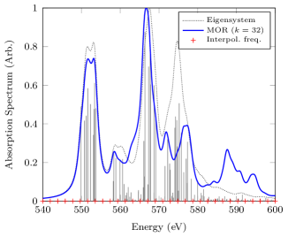
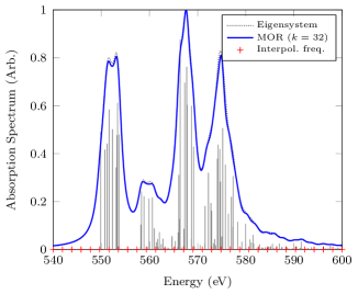
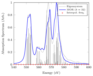
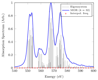
In the first experiment, we used a fixed order $k=32$ for the reduced order models and only changed the interpolation frequencies $\tau_{j}$, $j=1,2,\ldots,k$. We computed the absorption spectrum by algorithms 1 and 2 for both real $\tau_{j}=\omega_{j}$ and complex $\tau_{j}=\omega_{j}+i\eta$, where $\omega_{j}$ were uniformly selected in the energy window. The corresponding results are presented in fig. 2 and in the top part of table 1. Note that by using complex interpolation frequencies $\tau_{j}$, we obtained good approximations to the absorption spectrum from both algorithms 1 and 2 even with such a small model size. On the other hand, the use of real $\tau_{j}$ resulted in poor approximations for both algorithms. This is due to the fact that the (real) interpolation frequencies are often very close to the (real) eigenvalues of $(\mathbf{H},\mathbf{S})$ or $\mathbf{M}\mathbf{K}$, resulting in ill-conditioned linear systems to be solved. However, this can be avoided with complex interpolation frequencies.

Table 1: The effect of using real and complex interpolation frequencies $\tau_{j}$ on the MOR evaluation of XAS spectra for 5 H₂O clusters. Computational expense for algorithms 1 and 2. Here $k$ is the reduced order, GEMMs is the total number of matrix-matrix products, and the total wall-clock time is given in seconds.

Algorithm	$k$			GEMMs			Wall (s)
Algorithm 1: real $\tau_{j}$		32			1,052			19.76
Algorithm 1: complex $\tau_{j}$		32			776			40.97
Algorithm 2: real $\tau_{j}$		32			985			9.78
Algorithm 2: complex $\tau_{j}$		32			646			17.5
Algorithm 1: real $\tau_{j}$		218			7,440			137.01
Algorithm 1: complex $\tau_{j}$		87			2,285			115.50
Algorithm 2: real $\tau_{j}$		211			6,541			65.31
Algorithm 2: complex $\tau_{j}$		87			2,026			52.70
Conventional CPP (1,000 points)					18,126			538.90

Next, we repeated the previous experiment but chose the interpolation frequencies via the adaptive refinement strategy introduced in section 5. As the error estimates, we used the difference of the normalized absorption spectrum between two consecutive refinement levels. The tolerance was set to $0.01$, which corresponds to a 1 percent change in the overall absorption spectrum on the window $[540\,\mathrm{eV},600\,\mathrm{eV}]$. This resulted in reduced order models of different orders $k$, reported in the middle part of table 1. We observe that in terms of the order $k$, the use of complex interpolation frequencies has a significant advantage over the use of real frequencies. Further, we also observe that the adaptive refinement strategy for algorithms 1 and 2 resulted in very similar orders $k$ when the same type of interpolation frequencies are used.

The corresponding computational expense for the previous two experiments is reported in table 1 using various metrics. We observe that for both fixed and adaptive model orders, the computational cost required for algorithm 2 was significantly lower than that of algorithm 1. This is expected as both methods are mathematically equivalent and the former only deals with linear systems of half the dimension of the latter. Furthermore, although real interpolation frequencies allow us to solve only real linear systems, we observe that in case of adaptively chosen model orders, the drastic decrease in model order required for complex interpolation frequencies over real frequencies offsets this advantage. Finally, we note at the bottom of table 1 that the use of algorithm 2 with complex interpolation frequencies reduces the computational expense by a factor of almost 10 compared to conventional complex polarization propagator calculations on a fine grid.

6.2 Computational scaling

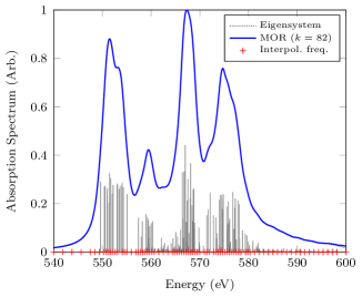
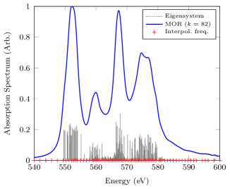
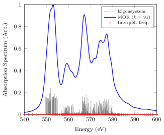
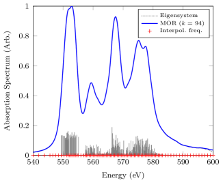
We now consider water clusters consisting of 5, 10, 15, 20, and 25 water molecules. The corresponding matrix dimensions are shown in table 2. The energy window $[540\,\mathrm{eV},600\,\mathrm{eV}]$ and damping factor $\eta=1\,\mathrm{eV}$ were the same as for the previous experiments. We computed the absorption spectrum via algorithm 2 with complex interpolation frequencies chosen adaptively. The obtained absorption spectra are shown in fig. 3.

(a) Water cluster 10 H₂O

(b) Water cluster 15 H₂O

(c) Water cluster 20 H₂O

(d) Water cluster 25 H₂O

Figure 3: Numerical experiments for the evaluation of the XAS spectrum of variably sized H₂O clusters via algorithm 2 with adaptively chosen complex interpolation frequencies. The MOR results are compared to the Lorentzian broadened poles of the propagator, labelled Eigensystem. A damping parameter of $1\,\mathrm{eV}$ was chosen both for the MOR calculations and the broadening factor of the Lorentzians for the reference.

Table 2: Numerical experiments for the evaluation of the XAS spectrum of variably sized H₂O clusters via algorithm 2 with adaptively chosen complex interpolation frequencies. Here, $\mathbf{M}\mathbf{K}$ is of dimension $n$ with $\#\lambda$ eigenvalues lying within the energy window $[540\,\mathrm{eV},600\,\mathrm{eV}]$. The comparisons are made for GMRES convergence tolerances of $10^{-4}$, $10^{-5}$, and $10^{-6}$, with $k$ as the reduced model order, GEMMs as the total number of matrix-matrix products, and the total wall-clock time is given in seconds.

Waters			GMRES tol = $10^{-4}$			GMRES tol = $10^{-5}$			GMRES tol = $10^{-6}$
#	$n$	#$\lambda$	$k$ GEMMs Wall (s)			$k$ GEMMs Wall (s)			$k$ GEMMs Wall (s)
5	3,250	394	76	968	27.2	87	1,654	43.4	87	2,025	52.7
10	13,000	1,456	99	1,749	636.2	83	2,404	867.1	82	3,235	1,157.0
15	29,250	3,183	99	2,221	4,141.8	82	2,946	5,511.9	82	4,018	7,534.4
20	52,000	5,524	123	2,742	14,665.8	89	3,317	17,807.0	91	4,594	25,656.5
25	81,250	8,530	123	2,610	34,128.8	95	3,694	47,697.1	94	5,020	65,284.1

The MOR results are given in table 2, where we present the orders $k$ of the reduced order models, the total number of GEMMs, and the total wall-clock time for different GMRES convergence tolerances. Firstly, we observe that the order $k$ of the reduced order models increases sub-linearly with the number of waters, whereas the number of eigenvalues inside the energy window, #$\lambda$, grows linearly with respect to the problem dimension. Secondly, the order $k$ decreases for increasing GMRES convergence tolerances. This is due to the fact that if we solve the linear systems less accurately, we match the moments less accurately and hence we need more interpolation points (a higher value of $k$) for the same accuracy of the reduced order model and the corresponding absorption spectra. Moreover, the order $k$ seems to stagnate around GMRES tolerance $10^{-5}$ and there were no visual differences any more between the obtained absorption spectra for GMRES tolerances $10^{-5}$ and $10^{-6}$.

(a) Wall time

(b) Total number of GEMMs

Figure 4: Cluster of H₂O molecules: MOR results for the absorption spectra computed via algorithm 2 with adaptively chosen complex interpolation frequencies. The comparisons are made for GMRES convergence tolerances of $10^{-4}$, $10^{-5}$, and $10^{-6}$.

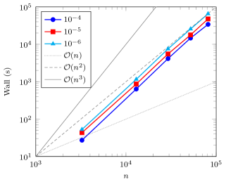
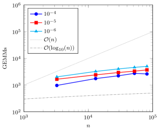
The total wall-clock time and number of GEMMs are also shown in fig. 4. The left figure illustrates that the wall-clock time scales quadratically with respect to the problem dimension, compared to a cubic scaling for a full diagonalization. Moreover, the right figure shows that the number of GEMMs only scales logarithmically, compared to an expected linear scaling for iterative eigensolvers since the number of eigenvalues inside the energy window grows linearly. It is worth noting that the vector space dimension of the linear problem also scales quadratically with system size.

6.3 Effect of damping factor

We examine the effect of the damping factor on the overall effectiveness of the proposed MOR algorithm in the low damping limit. We revisit the case of water clusters containing 5 water molecules from the previous subsections over the same energy widow. Specifically, we examine the effect on the damping parameter $\eta\in[0.1,1]\,\mathrm{eV}$ on the model order required to achieve a convergence of 1 percent in the absorption spectrum. The MOR results were obtains via algorithm 2 using adaptively chosen complex interpolation frequencies. The resulting spectra are presented in fig. 5(a)–(c).

(a) $\eta=0.5\,\mathrm{eV}$

(b) $\eta=0.3\,\mathrm{eV}$

(c) $\eta=0.1\,\mathrm{eV}$

(d) $k$ as a function of $\eta$

Figure 5: Numerical experiments for the evaluation of the XAS spectrum of 5 H₂O clusters by algorithm 2 using different damping factors $\eta$. (a)–(c) The MOR results are compared to the Lorentzian broadened poles of the propagator, labelled Eigensystem. (d) Effect of the damping factor $\eta$ on the reduced model order $k$.

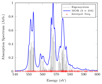
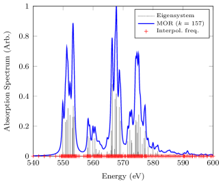
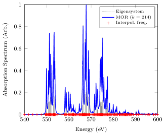
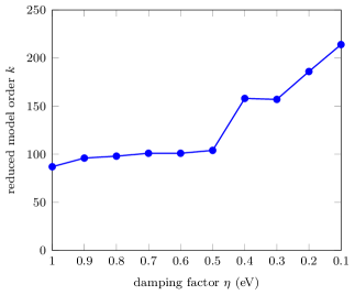
The effect of the damping factor on the automatically selected model order is illustrated in fig. 5(d). In this figure, we observe that by decreasing the damping factor the reduced model order $k$ first remains almost constant until $0.5\,\mathrm{eV}$ and then slightly starts to increase for smaller values of $\eta$. Even in the low damping limit ($0.1\,\mathrm{eV}$), when the obtained absorption spectrum is exceptionally complicated and oscillatory relative to the previous experiments ($1\,\mathrm{eV}$), the required model order is still well within the realm of practicality for routine calculations. Thus the proposed MOR algorithm may be used as a general procedure which requires no assumption of (the smoothness of) the underlying absorption spectrum.

7 Conclusion

In this work, we have presented a novel, adaptive algorithm for the ab initio prediction of the absorption spectrum based on model order reduction techniques applied to the quantum propagator. While this approach is general to any spectral domain, the power of the proposed method is in those spectral domains which are dense and interior in the propagator’s eigenspectrum. The accuracy and efficiency of this method to predict the X-Ray absorption spectrum have been demonstrated using a series of water clusters. Water clusters were chosen as an especially challenging case study as the propagator is spectrally dense in the spectral neighborhood of the water’s oxygen $K$-Edge. The numerical experiments have shown that complex interpolation frequencies should be preferred over real ones and that in this case the order of the reduced order models only slightly increases with the problem dimension, in contrast to the rapid growth of the number of eigenvalues inside the energy window. Moreover, the wall-clock time for the proposed model order reduction algorithm scales only quadratically with respect to the dimension of the problem, compared to cubic scaling for eigenvalue based algorithms. Further, it was shown that, even in the limit of highly oscillatory and low damping absorption spectra, the proposed algorithm remains practical and thus may be treated as agnostic to the underlying nature of the spectrum. While results were presented only for the TD-HF method, the proposed adaptive MOR algorithm is general to any choice reference, propagator, or perturbation. Further, although it is not expressly considered in this work, this technique is well suited for parallelism on a massive scale as each of the linear system solutions is completely independent from the other, thus allowing for minimal communication. With the proposed MOR algorithm, routine study of X-Ray absorption spectra for medium-to-large sized systems is simplified.

This work was partly supported by the Scientific Discovery through Advanced Computing (SciDAC) program (R. V. B., C. Y. and E. G. N.) and the IDREAM Energy Frontier Research Center (D. B. W.-Y., J. M. K. and X. L.), funded by U.S. Department of Energy, Office of Science, Advanced Scientific Computing Research and Basic Energy Sciences. R. V. B. is a Postdoctoral Fellow of the Research Foundation - Flanders (12J2217N). The development of the Chronus Quantum software is supported by the National Science Foundation (CHE-1565520 to X. L.). The authors thank the National Energy Research Scientific Computing (NERSC) center for making computational resources available to them. Further, this work was facilitated though the use of advanced computational, storage, and networking infrastructure provided by the Hyak supercomputer system at the University of Washington. The authors are also grateful to Dr. Meiyue Shao for helpful discussions.

References

- Stöhr 2013 Stöhr, J. NEXAFS spectroscopy; Springer Science & Business Media, 2013; Vol. 25
- Yannoulis et al. 1987 Yannoulis, P.; Dudde, R.; Frank, K.; Koch, E. Orientation of Aromatic Hydrocarbons on Metal Surfaces as Determined by NEXAFS. Surf. Sci. 1987, 189, 519–528
- Aygül et al. 2012 Aygül, U.; Batchelor, D.; Dettinger, U.; Yilmaz, S.; Allard, S.; Scherf, U.; Peisert, H.; Chassé, T. Molecular Orientation in Polymer Films for Organic Solar Cells Studied by NEXAFS. J. Phys. Chem. C 2012, 116, 4870–4874
- Shadle et al. 1995 Shadle, S. E.; Hedman, B.; Hodgson, K. O.; Solomon, E. I. Ligand K-Edge X-Ray Absorption Spectroscopic Studies. Metal-Ligand Covalency in a Series of Transition Metal Tetrachlorides. J. Am. Chem. Soc. 1995, 117, 2259–2272
- DuBois et al. 2000 DuBois, J. L.; Mukherjee, P.; Stack, T.; Hedman, B.; Solomon, E. I.; Hodgson, K. O. A Systematic K-Edge X-Ray Absorption Spectroscopic Study of Cu (III) Sites. J. Am. Chem. Soc. 2000, 122, 5775–5787
- Chen et al. 2001 Chen, L. X.; Jäger, W. J.; Jennings, G.; Gosztola, D. J.; Munkholm, A.; Hessler, J. P. Capturing a photoexcited molecular structure through time-domain X-ray absorption fine structure. Science 2001, 292, 262–264
- Chen et al. 2016 Chen, L. X.; Shelby, M. L.; Lestrange, P. J.; Jackson, N. E.; Haldrup, K.; Mara, M. W.; Stickrath, A. B.; Zhu, D.; Lemke, H.; Chollet, M.; Hoffman, B. M.; Li, X. Imaging Ultrafast Excited State Pathways in Transition Metal Complexes by X-ray Transient Absorption and Scattering using X-ray Free Electron Laser Source. Faraday Discuss. 2016, 194, 639–658
- Shelby et al. 2016 Shelby, M. L.; Lestrange, P. J.; Jackson, N. E.; Haldrup, K.; Mara, M. W.; Stickrath, A. B.; Zhu, D.; Lemke, H.; Chollet, M.; Hoffman, B. M.; Li, X.; Chen, L. X. Ultrafast Excited State Relaxation of a Metalloporphyrin Revealed by Femtosecond X-ray Absorption Spectroscopy. J. Am. Chem. Soc. 2016, 138, 8752–8764
- Li et al. 2005 Li, X.; Smith, S. M.; Markevitch, A. N.; Romanov, D. A.; Levis, R. J.; Schlegel, H. B. A Time-dependent Hartree-Fock Approach for Studying the Electronic Optical Response of Molecules in Intense Fields. Phys. Chem. Chem. Phys. 2005, 7, 233–239
- Li and Tully 2007 Li, X.; Tully, J. C. Ab initio Time-resolved Density Functional Theory for Lifetimes of Excited Adsorbate States at Metal Surfaces. Chem. Phys. Lett. 2007, 439, 199
- Liang et al. 2011 Liang, W.; Chapman, C. T.; Li, X. Efficient First-principles Electronic Dynamics. J. Chem. Phys. 2011, 134, 184102
- Lopata et al. 2012 Lopata, K.; Van Kuiken, B. E.; Khalil, M.; Govind, N. Linear-response and real-time time-dependent density functional theory studies of core-level near-edge x-ray absorption. J. Chem. Theor. Comput. 2012, 8, 3284–3292
- Bruner et al. 2016 Bruner, A.; LaMaster, D.; Lopata, K. Accelerated broadband spectra using transition dipole decomposition and Padé approximants. J. Chem. Theor. Comput. 2016, 12, 3741–3750
- Oddershede et al. 1984 Oddershede, J.; Jørgensen, P.; Yeager, D. L. Polarization Propagator Methods in Atomic and Molecular Calculations. Comp. Phys. Rep. 1984, 2, 33–92
- Olsen et al. 1988 Olsen, J.; Jensen, H. J. A.; Jørgensen, P. Solution of the large matrix equations which occur in response theory. J. Comput. Phys. 1988, 74, 265–282
- Monkhorst 1977 Monkhorst, H. J. Calculation of Properties with the Coupled-Cluster Method. Int. J. Quant. Chem. 1977, 12, 421–432
- Koch and Jørgensen 1990 Koch, H.; Jørgensen, P. Coupled Cluster Response Functions. J. Chem. Phys. 1990, 93, 3333–3344
- Stanton and Bartlett 1993 Stanton, J. F.; Bartlett, R. J. The Equation of Motion Coupled-Cluster Method. A Systematic Biorthogonal Approach to Molecular Excitation Energies, Transition Probabilities, and Excited State Properties. J. Chem. Phys. 1993, 98, 7029–7039
- Comeau and Bartlett 1993 Comeau, D. C.; Bartlett, R. J. The Equation-of-Motion Coupled-Cluster Method. Applications to Open-and Closed-Shell Reference States. Chem. Phys. Lett. 1993, 207, 414–423
- Wenzel et al. 2014 Wenzel, J.; Wormit, M.; Dreuw, A. Calculating X-ray absorption spectra of open-shell molecules with the unrestricted algebraic-diagrammatic construction scheme for the polarization propagator. J. Chem. Theor. Comput. 2014, 10, 4583
- Wenzel et al. 2014 Wenzel, J.; Wormit, M.; Dreuw, A. Calculating core-level excitations and X-ray absorption spectra of large and medium sized closed-shell molecules with the algebraic-diagrammatic construction scheme for the polarization propagator. J. Chem. Theor. Comput. 2014, 35, 1900
- Christiansen et al. 1998 Christiansen, O.; Jørgensen, P.; Hättig, C. Response Functions from Fourier Component Variational Perturbation Theory Applied to a Time-Averaged Quasienergy. Int. J. Quant. Chem. 1998, 68, 1–52
- Ring and Schuck 2004 Ring, P.; Schuck, P. The Nuclear Many-Body Problem; Springer Science & Business Media, 2004
- Jørgensen and Simmons 1981 Jørgensen, P.; Simmons, J. Second Quantization–Based Methods in Quantum Chemistry; Academic Press Inc., 1981
- Rowe 1968 Rowe, D. Equations-of-Motion Method and the Extended Shell Model. Rev. Mod. Phys. 1968, 40, 153
- Casida 1995 Casida, M. E. In Recent Advances in Density Functional Methods:(Part I); Chong, D. P., Ed.; World Scientific; Singapore, 1995; Vol. 1; pp 155–193
- Dreuw and Head-Gordon 2005 Dreuw, A.; Head-Gordon, M. Single-Reference Ab Initio Methods for the Calculation of Excited States of Large Molecules. Chem. Rev. 2005, 105, 4009–4037
- Helgaker et al. 2012 Helgaker, T.; Coriani, S.; Jørgensen, P.; Kristensen, K.; Olsen, J.; Ruud, K. Recent Advances in Wave Function-Based Methods of Molecular-Property Calculations. Chem. Rev. 2012, 112, 543–631
- Shavitt and Bartlett 2009 Shavitt, I.; Bartlett, R. J. Many-Body Methods in Chemistry and Physics: MBPT and Coupled-Cluster Theory; Cambridge university press, 2009
- Liang et al. 2011 Liang, W.; Fischer, S. A.; Frisch, M. J.; Li, X. Energy-Specific Linear Response TDHF/TDDFT for Calculating High-Energy Excited States. J. Chem. Theor. Comput. 2011, 7, 3540–3547
- Lestrange et al. 2015 Lestrange, P. J.; Nguyen, P. D.; Li, X. Calibration of Energy-Specific TDDFT for Modeling K-edge XAS Spectra of Light Elements. J. Chem. Theor. Comput. 2015, 11, 2994–2999
- Peng et al. 2015 Peng, B.; Lestrange, P. J.; Goings, J. J.; Caricato, M.; Li, X. Energy-Specific Equation-of-Motion Coupled-Cluster Methods for High-Energy Excited States: Application to K-edge X-ray Absorption Spectroscopy. J. Chem. Theor. Comput. 2015, 11, 4146–4153
- Stener et al. 2003 Stener, M.; Fronzoni, G.; De Simone, M. Time Dependent Density Functional Theory of Core Electrons Excitations. Chem. Phys. Lett. 2003, 373, 115–123
- Ray et al. 2007 Ray, K.; DeBeer George, S.; Solomon, E. I.; Wieghardt, K.; Neese, F. Description of the Ground-State Covalencies of the Bis (dithiolato) Transition-Metal Complexes from X-ray Absorption Spectroscopy and Time-Dependent Density-Functional Calculations. Chem. Eur. J. 2007, 13, 2783–2797
- Besley and Asmuruf 2010 Besley, N. A.; Asmuruf, F. A. Time-Dependent Density Functional Theory Calculations of the Spectroscopy of Core Electrons. Phys. Chem. Chem. Phys. 2010, 12, 12024–12039
- Davidson 1975 Davidson, E. R. The Iterative Calculation of a Few of the Lowest Eigenvalues and Corresponding Eigenvectors of Large Real–Symmetric Matricies. J. Comput. Phys. 1975, 17, 87
- Morgan and Scott 1986 Morgan, R. B.; Scott, D. S. Generalizations of Davidson’s Method for Computing Eigenvalues of Sparse Symmetric Matricies. SIAM J. Sci. Statist. Comput. 1986, 7, 817–825
- Morgan 1992 Morgan, R. B. Generalizations of Davidson’s Method for Computing Eigenvalues of Large Non–Symmetric Matricies. J. Comput. Phys. 1992, 101, 287–291
- Zuev et al. 2015 Zuev, D.; Vecharynski, E.; Yang, C.; Orms, N.; Krylov, A. I. New Algorithms for Iterative Matrix-Free Eigensolvers in Quantum Chemistry. J. Comput. Chem. 2015, 36, 273–284
- Coriani et al. 2012 Coriani, S.; Fransson, T.; Christiansen, O.; Norman, P. Asymmetric-Lanczos-chain-driven implementation of electronic resonance convergent coupled-cluster linear response theory. J. Chem. Theor. Comput. 2012, 8, 1616–1628
- Fransson et al. 2013 Fransson, T.; Coriani, S.; Christiansen, O.; Norman, P. Carbon X-ray Absorption Spectra of Fluoroethenes and Acetone: A Study at the Coupled Cluster, Density Functional, and Static-exchange Levels of Theory. J. Chem. Phys. 2013, 138, 124311
- Kauczor et al. 2013 Kauczor, J.; Norman, P.; Christiansen, O.; Coriani, S. Communication: A Reduced-Space Algorithm for the Solution of the Complex Linear Response Equations used in Coupled Cluster Damped Response Theory. 2013
- Marques et al. 2012 Marques, M. A.; Maitra, N. T.; Nogueira, F. M.; Gross, E. K.; Rubio, A. Fundamentals of Time-Dependent Density Functional Theory; Springer Science & Business Media, 2012; Vol. 837; Chapter 7
- Norman et al. 2001 Norman, P.; Bishop, D. M.; Jørgen Aa. Jensen, H.; Oddershede, J. Near-Resonant Absorption in the Time-Dependent Self-Consistent Field and Multiconfigurational Self-Consistent Field Approximations. J. Chem. Phys. 2001, 115, 10323–10334
- Fahleson et al. 2016 Fahleson, T.; Ågren, H.; Norman, P. A Polarization Propagator for Nonlinear X-ray Spectroscopies. J. Phys. Chem. Lett. 2016, 7, 1991–1995
- Coriani et al. 2012 Coriani, S.; Christiansen, O.; Fransson, T.; Norman, P. Coupled-Cluster Response Theory for Near-Edge X-Ray-Absorption Fine Structure of Atoms and Molecules. Phys. Rev. A 2012, 85, 022507
- Linares et al. 2010 Linares, M.; Stafström, S.; Rinkevicius, Z.; Ågren, H.; Norman, P. Complex Polarization Propagator Approach in the Restricted Open-Shell, Self-Consistent Field Approximation: The Near K-Edge X-ray Absorption Fine Structure Spectra of Allyl and Copper Phthalocyanine. J. Phys. Chem. B 2010, 115, 5096–5102
- Ekström et al. 2006 Ekström, U.; Norman, P.; Carravetta, V.; Ågren, H. Polarization Propagator for X-ray Spectra. Phys. Rev. Lett. 2006, 97, 143001
- Fransson et al. 2016 Fransson, T.; Burdakova, D.; Norman, P. K-and L-Edge X-Ray Absorption Spectrum Calculations of Closed-Shell Carbon, Silicon, Germanium, and Sulfur Compounds using Damped Four-Component Density Functional Response Theory. Phys. Chem. Chem. Phys. 2016, 18, 13591–13603
- Norman et al. 2015 Norman, P.; Parello, J.; Polavarapu, P. L.; Linares, M. Predicting Near-UV Electronic Circular Dichroism in Nucleosomal DNA by Means of DFT Response Theory. Phys. Chem. Chem. Phys. 2015, 17, 21866–21879
- Villaume et al. 2010 Villaume, S.; Saue, T.; Norman, P. Linear Complex Polarization Propagator in a Four-Component Kohn–Sham Framework. J. Chem. Phys. 2010, 133, 064105
- Antoulas 2005 Antoulas, A. C. In Advances in Design and Control 6; Ralph C. Smith North Carolina State University,, Ed.; Advances in Design and Control 6; SIAM, 2005; p 479
- Benner et al. 1998 Benner, P.; Mehrmann, V.; Xu, H. A numerically stable, structure preserving method for computing the eigenvalues of real Hamiltonian or symplectic pencils. Numer. Math. 1998, 78, 329–358
- Bai and Li 2012 Bai, Z.; Li, R.-C. Minimization principles for the linear response eigenvalue problem I: Theory. SIAM J. Mat. Anal. Appl. 2012, 33, 1075–1100
- Shao et al. 2016 Shao, M.; da Jornada, F. H.; Yang, C.; Deslippe, J.; Louie, S. G. Structure preserving parallel algorithms for solving the Bethe–Salpeter eigenvalue problem. Linear Algebra Appl. 2016, 488, 148–167
- Weiss et al. 1993 Weiss, H.; Ahlrichs, R.; Häser, M. A Direct Algorithm for Self-Consistent-Field Linear Response Theory and Application to C60: Excitation Energies, Oscillator Strengths, and Frequency-Dependent Polarizabilities. J. Chem. Phys. 1993, 99, 1262–1270
- Stratmann et al. 1998 Stratmann, R. E.; Scuseria, G. E.; Frisch, M. J. An Efficient Implementation of Time-Dependent Density-Functional Theory for the Calculation of Excitation Energies of Large Molecules. J. Chem. Phys. 1998, 109, 8218–8224
- 58 Brabec, J.; Lin, L.; Shao, M.; Govind, N.; Yang, C.; Saad, Y.; Ng, E. G. Efficient Algorithms for Estimating the Absorption Spectrum within Linear Response TDDFT. J. Chem. Theor. Comput. 11, 5197–5208
- Li et al. 2017 Li, X.; Valeev, E. F.; Williams-Young, D.; Ding, F.; Liu, H.; Goings, J.; Petrone, A.; Lestrange, P. Chronus Quantum, Beta Version. 2017; http://www.chronusquantum.org
- Walker 1988 Walker, H. F. Implementation of the GMRES Method using Householder Transformations. SIAM J. Sci. Stat. Comp. 1988, 9, 152–163
- Shao et al. 2016 Shao, M.; Aktulga, H. M.; Yang, C.; Ng, E. G.; Maris, P.; Vary, J. P. Accelerating Nuclear Configuration Interaction Calculations through a Preconditioned Block Iterative Eigensolver. arXiv 2016, abs/1609.01689
- McLachlan and Ball 1964 McLachlan, A.; Ball, M. Time-Dependent Hartree–Fock Theory for Molecules. Rev. Mod. Phys. 1964, 36, 844
- Harris 1969 Harris, R. A. Oscillator Strengths and Rotational Strengths in Hartree–Fock Theory. J. Chem. Phys. 1969, 50, 3947–3951
- Yeager et al. 1975 Yeager, D.; Nascimento, M.; McKoy, V. Some Applications of Excited-State-Excited-State Transition Densities. Phys. Rev. A 1975, 11, 1168
- Shao and Yang 2016 Shao, M.; Yang, C. BSEPACK User’s Guide. 2016; https://sites.google.com/a/lbl.gov/bsepack/
- Stöhr 2013 Stöhr, J. NEXAFS Spectroscopy; Springer Science & Business Media, 2013; Vol. 25