A multiple model and observation 10m wind climatology for the Gulf of California

Abstract

Seven data sources are analysed and combined to form a surface wind speed climatology for the Gulf of California.

CICESE (Centro de Investigación Científica y de Educación Superior de Ensenada), Departamento de Oceanografía Física, Carretera Ensenada-Tijuana 3918, Ensenada BC 22860, MEXICO, mgross@cicese.mx

Dataset

1. name of dataset: 10m Wind Speed Climatology for the Gulf of California
   data centre: figshare
   DOI:10.6084/m9.figshare.4037235
   Identifier: xxxxx
   Creator: Markus Gross
   Title: xxxxxx
   Publisher: xxxxxx
   Publication year: 2016
   Resource type: netcdf and ASCII files
   Version: 3.0

1 Introduction

Climatologically correct data for $10$m wind speeds are important for a variety of applications, such as forcing regional ocean models, which then in turn can be used to analyse tracer transport, biological activity, renewable energy resources and the analysis of climate anomalies, for example. However, for the Gulf of California (GOC) to date no single, reliable source of data exits to provide guidance for such studies. Therefore, in this work the data from seven data sources was combined to generate seasonal climatological means. These are then provided in two formats: A two dimensional gridded dataset of the temporally averaged data and temporally-spatially averaged values.

1.1 Geographic domains

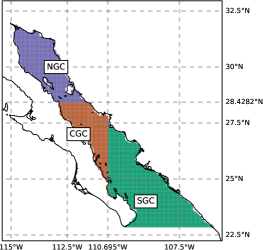
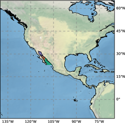
The geographic domain is limited in the west by the Baja California peninsular and in the east by the Mexican mainland. In the south the data is considered until the last land point in the Baja California peninsular. This domain is then further subdivided (sub-domains) into the Northern (NGC), Central (CGC) and Southern Gulf (SGC), as shown in Figure 1. The southern limit to the NGC domain is latitude $28.428207\degree$. CGC and SGC are divided by longitude $-110.695\degree$.

(a)

(b)

Figure 1: Geographic domains for spatial averages

2 Data production methods

In the following the individual source dataset are described. Then the processing steps to obtain the temporal and spatial mean dataset are presented.

2.1 Source datasets

Four numerical models and three observational products were combined in this study. The observational products were:

1. The Cross-Calibrated Multi-Platform observational product (CCMP),

2. Global Wind, L4 2007-2012 Climatology (WIND_GLO),

3. Global Ocean - Wind Analysis - Blended Advanced Scatterometer (ASCAT) - Special Sensor Microwave Imager (SSM/I) (CERSAT),

and the numerical models used were

1. UK Met Office Unified Model 8 UK on PRACE (the Partnership for Advanced Computing in Europe) - weather-resolving Simulations of Climate for global Environmental risk (UPSCALE),

2. Climate forecast system reanalysis (CFSR),

3. National Centers for Environmental Prediction (NCEP) North American Regional Reanalysis (NARR) and the

4. North American Mesoscale model (NAM).

The time coverage of the respective datasets is shown in Figure 2 and details about each dataset are provided below.

Figure 2: Data source time coverage

2.1.1 UPSCALE

The UPSCALE dataset is the result of a global N512 (512 is the number of 2 grid length waves that can be supported in the Eeast-West direction, hence N512 yields 1024x768 grid points East-West x North-South) UPSCALE project. It is based on the Hadley Centre Global Environment Model version 3 (HadGEM3) - Global Atmosphere (GA) 3.0 configuration of the Met Office Unified Model (MetUM) version 8.0, combined with the Global Land (GL) 3.0 configuration of the Joint UK Land Environment Simulator (JULES) community land surface model, as documented in Walters et al. (2011). The model was configured to reproduce the present climate for the period Feb 1985 to Dec 2011. More detailed information about the UPSCALE model simulations is available in Mizielinski et al. (2014); Donlon et al. (2012). Instantaneous winds, obtained every three hours, are averaged over the respective seasons. The resolution of the model was $0.23438\degree$ in latitude and $0.3516\degree$ degrees in longitude.

2.1.2 NAM-ANL

The North American Mesoscale Forecast System (NAM) dataset is a numerical weather prediction (NWP) dataset produced by the US National Weather Service - National Centers for Environmental Prediction (NCEP), for North America, using the MESO ETA Model, Black (1994). The grid resolution is 12km using the Advanced Weather Interactive Processing System (AWIPS) lambert conformal grid over the Contiguous United States (CONUS). The raw data was re-gridded (using bi-linear interpolation) onto a lat-long grid with uniform $0.05\degree$ grid spacing. Instantaneous winds, obtained every six hours, are averaged over the respective seasons.

2.1.3 NARR

NCEP North American Regional Analysis (NARR) dataset, Mesinger et al. (2006), is a regional reanalysis dataset. The monthly means of the original dataset are averaged over the respective seasons. 450 monthly mean winds at $10$m were used. The NARR model uses the NCEP Eta Model (32km Lambert Conformal/45 layer) combined with the Regional Data Assimilation System (RDAS). The resulting dataset improves significantly on the accuracy of temperature, winds and precipitation compared to the NCEP-DOE Global Reanalysis 2, Kanamitsu et al. (2002). Here the data was re-gridded onto a $0.2\degree$ uniform lat-long grid.

2.1.4 CCMP

The Cross-Calibrated Multi-Platform (CCMP) ocean surface wind vector analyses (Atlas et al. (2011, 1996)) provide a consistent, gap-free long-term time-series from July 1987 through June 2011. The CCMP datasets combine cross-calibrated satellite winds using a Variational Analysis Method (VAM), Hoffman et al. (2003), to produce a $0.25\degree$ gridded analysis. The CCMP dataset uses satellite winds derived by Remote Sensing Systems (RSS) from a number of microwave satellite instruments. RSS applies a sea-surface emissivity model and radiative transfer function to derive surface winds. Wind speeds and directions from microwave scatterometers (including NASA’s Quik Scatterometer (QuikScat) and its SeaWinds instrument) are also considered. Both radiometer and scatterometer data are validated against ocean moored buoys. The VAM combines the RSS data with in situ measurements and a starting estimate of the wind field. The European Center for Medium-Range Weather Forecasts (ECMWF) ERA-40 Reanalysis is used as the first-guess from 1987 to 1998. The ECMWF Operational analysis is used from January 1999 onward. All wind observations and analysis fields are referenced to a height of $10$ meters. The landmask for this dataset was generated from the topography of the UPSCALE dataset, re-gridded to the CCMP resolution.

2.1.5 CSFR- CLIMATE FORECAST SYSTEM REANALYSIS

The CFSR, Saha et al. (2010), includes coupling of atmosphere and ocean during the generation of the 6 hour guess field, an interactive sea-ice model, and assimilation of satellite radiances. The CFSR global atmosphere resolution is $\approx 38$ km (T382) with $64$ vertical levels. The global ocean is $0.25\degree$ at the equator, extending to a global $0.5\degree$ beyond the tropics, with $40$ vertical levels. Ocean-atmosphere interactions are not used directly. Rather the information is used for background information. The actual reanalysis is uncoupled. $117$ monthly averages of the six-hourly analyses were included in this study.

2.1.6 CERSAT (V5 and V3)

The CERSAT (Centre ERS d’Archivage et de Traitement) Global Blended Mean Wind Fields V5 include wind components (meridional and zonal), wind module and wind stress. They are estimated from scatterometers ASCAT and Oceansat-2 Scatterometer (OSCAT) retrievals and from ECMWF operational wind analysis with a horizontal resolution of $0.25\degree$ and $6$ hours in time. The estimation and calibration of the wind product made use of ASCAT and OSCAT scatterometer swath winds, ECMWF wind analysis, and moored buoy data. For the period 2012-2015 the V3 dataset was used.

2.1.7 GLO

The Global Ocean CERSAT surface wind climatology, covering the years 2007-2012, is estimated from ASCAT retrievals Bentamy and Fillon (2012). The analyses are estimated as monthly averaged data with spatial resolution of $0.25\degree$ in latitude and longitude.

2.2 Processing of source data

First the data was averaged in time. Individual netcdf files are provided with the seasonal temporal averages, for each source dataset. Then the spatial averages were computed. At first this averaging was performed individually for each dataset. Following a selection procedure outlined below the selected averages were then combined to form one single representative value for each season and geographic sub-domain, respectively.

2.2.1 Temporal-Spatial averages of the datasets

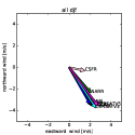
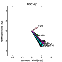
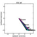
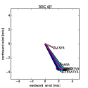
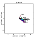
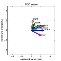
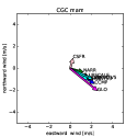
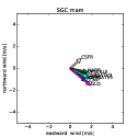
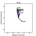
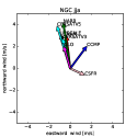
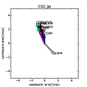
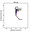
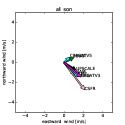
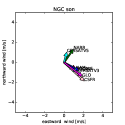
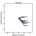
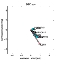
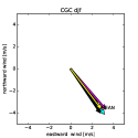
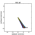
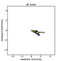
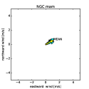
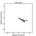
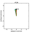
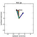
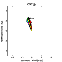
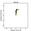
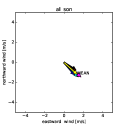
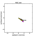
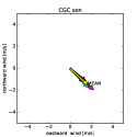
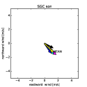
The datasets were averaged in space according to the three regions presented above. No particular weighting was applied as the difference in areas covered north to south is small. The resulting average wind speed and direction is illustrated in Figure 3 for each sub-domain and season.

(a)

(b)

(c)

(d)

(e)

(f)

(g)

(h)

(i)

(j)

(k)

(l)

(m)

(n)

(o)

(p)

Figure 3: Temporal-spatial averages

2.2.2 Data selection

From Figure 3 it is clear that whilst there is some similarity between the datasets there are also severe outliers. With the aim of generating “best data” temporal-spatial averages and recommending unique values the datasets were selected using two criteria:

1. Select the datasets with a wind direction, $\alpha$, of

   $$\overline{\alpha}-\sigma_{\alpha}<\alpha<\overline{\alpha}+\sigma,$$ (1)

   where $\sigma_{\alpha}$ is the standard deviation and $\overline{\alpha}$ is the mean of the wind direction of all datasets, for the particular sub-domain and season. This step eliminates the sever outliers apparent in Figure 3.

2. From this subset datasets which have wind velocity magnitudes (wind speeds), $v$, that are

   $$\overline{v}-\sigma_{v}<v<\overline{v}+\sigma_{v},$$ (2)

   where, as before, $\sigma_{v}$ is the standard deviation and $\overline{v}$ is the mean of the wind speed across all datasets selected by criteria one, were selected.

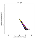
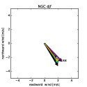
The result of this selection process is shown in Table 1, for all seasons and areas. The “X” entry denotes that the dataset was retained. First according to the angle criterion, Equation 1, and then subsequently by the speed criterion, Equation 2. The resulting means across the retained datasets are summarised in Table 2 and illustrated graphically in Figure 4.

Season	Area	crit	UPSCALE	NAM	NARR	CCMP	CSFR	CERSAT V5	CERSAT V3	GLO
djf	all	angle	X	X	X	X		X	X	X
		speed	X	X		X		X	X	X
	NGC	angle	X	X	X	X		X	X	X
		speed	X	X		X			X	X
	CGC	angle	X	X	X	X		X	X	X
		speed	X	X		X			X	X
	SGC	angle	X	X	X	X		X	X	X
		speed	X	X		X		X		X
mam	all	angle	X	X	X	X		X	X	X
		speed	X	X		X		X	X
	NGC	angle	X	X		X		X	X
		speed	X	X				X	X
	CGC	angle	X	X	X	X		X	X	X
		speed	X	X		X		X	X
	SGC	angle	X	X	X	X		X	X	X
		speed		X	X	X		X	X
jja	all	angle	X	X	X	X		X	X	X
		speed	X	X				X	X
	NGC	angle	X	X	X	X		X	X	X
		speed	X	X		X			X
	CGC	angle	X	X	X	X		X	X	X
		speed	X	X	X				X	X
	SGC	angle	X	X	X	X		X	X	X
		speed	X	X				X	X	X
son	all	angle	X	X		X	X		X	X
		speed	X	X		X			X	X
	NGC	angle	X	X		X	X		X	X
		speed		X		X			X	X
	CGC	angle	X	X		X	X		X	X
		speed	X	X		X			X	X
	SGC	angle	X	X		X	X		X	X
		speed	X	X		X			X	X

Table 1: Selected dataset according to the criteria (crit) Equation 1 (angle) and Equations 1 and 2 (speed subsequent to angle)

Season	Area	speed [m/s]	angle [deg]
djf	all	4.25	145.88
	NGC	3.3	142.38
	CGC	4.62	141.84
	SGC	4.42	148.27
mam	all	1.73	107.53
	NGC	1.31	61.63
	CGC	2.2	117.8
	SGC	1.89	115.74
jja	all	2.6	-6.51
	NGC	2.91	-0.01
	CGC	2.45	-17.39
	SGC	2.21	2.5
son	all	1.82	130.9
	NGC	1.79	121.68
	CGC	2.21	132.07
	SGC	1.85	133.93

Table 2: spatial temporal means

(a)

(b)

(c)

(d)

(e)

(f)

(g)

(h)

(i)

(j)

(k)

(l)

(m)

(n)

(o)

(p)

Figure 4: Temporal-spatial averages of selected dataset (same colors as in Figure 3) and mean (yellow)

3 Dataset location and format

The dataset is available from figshare. It comprises eight netcdf files, containing the temporally averaged fields alongside their lat-long coordinates. The temporal-spatial means are provided as plain ASCII file.

4 Dataset use and reuse

This dataset now enables the use for forcing data in oceanographic models, the analysis of climatological anomalies and their impacts on the gulf dynamics and transport processes. It also allows for a systematic analysis of the impact of wind forcing on the Gulf.

References

- Atlas et al. [1996] R. Atlas, R. N. Hoffman, S. C. Bloom, J. C. Jusem, and J. Ardizzone. A multiyear global surface wind velocity dataset using ssm/i wind observations. Bulletin of the American Meteorological Society, 77(5):869–882, 1996. doi: 10.1175/1520-0477(1996)077<0869:AMGSWV>2.0.CO;2. URL http://dx.doi.org/10.1175/1520-0477(1996)077<0869:AMGSWV>2.0.CO;2.
- Atlas et al. [2011] Robert Atlas, Ross N. Hoffman, Joseph Ardizzone, S. Mark Leidner, Juan Carlos Jusem, Deborah K. Smith, and Daniel Gombos. A cross-calibrated, multiplatform ocean surface wind velocity product for meteorological and oceanographic applications. Bulletin of the American Meteorological Society, 92(2):157–174, 2011. doi: 10.1175/2010BAMS2946.1. URL http://dx.doi.org/10.1175/2010BAMS2946.1.
- Bentamy and Fillon [2012] Abderrahim Bentamy and Denis Croize Fillon. Gridded surface wind fields from metop/ascat measurements. International Journal of Remote Sensing, 33(6):1729–1754, 2012. doi: 10.1080/01431161.2011.600348. URL http://dx.doi.org/10.1080/01431161.2011.600348.
- Black [1994] Thomas L. Black. The new nmc mesoscale eta model: Description and forecast examples. Weather and Forecasting, 9(2):265–278, 1994. doi: 10.1175/1520-0434(1994)009<0265:TNNMEM>2.0.CO;2. URL http://dx.doi.org/10.1175/1520-0434(1994)009<0265:TNNMEM>2.0.CO;2.
- Donlon et al. [2012] Craig J. Donlon, Matthew Martin, John Stark, Jonah Roberts-Jones, Emma Fiedler, and Werenfrid Wimmer. The operational sea surface temperature and sea ice analysis (ostia) system. Remote Sensing of Environment, 116(0):140 – 158, 2012. ISSN 0034-4257. doi: http://dx.doi.org/10.1016/j.rse.2010.10.017. URL http://www.sciencedirect.com/science/article/pii/S0034425711002197. Advanced Along Track Scanning Radiometer(AATSR) Special Issue.
- Hoffman et al. [2003] R. N. Hoffman, S. M. Leidner, J. M. Henderson, R. Atlas, J. V. Ardizzone, and S. C. Bloom. A two-dimensional variational analysis method for nscat ambiguity removal: Methodology, sensitivity, and tuning. Journal of Atmospheric and Oceanic Technology, 20(5):585–605, 2003. doi: 10.1175/1520-0426(2003)20<585:ATDVAM>2.0.CO;2. URL http://dx.doi.org/10.1175/1520-0426(2003)20<585:ATDVAM>2.0.CO;2.
- Kanamitsu et al. [2002] Masao Kanamitsu, Wesley Ebisuzaki, Jack Woollen, Shi-Keng Yang, J. J. Hnilo, M. Fiorino, and G. L. Potter. Ncep–doe amip-ii reanalysis (r-2). Bulletin of the American Meteorological Society, 83(11):1631–1643, 2002. doi: 10.1175/BAMS-83-11-1631. URL http://dx.doi.org/10.1175/BAMS-83-11-1631.
- Mesinger et al. [2006] Fedor Mesinger, Geoff DiMego, Eugenia Kalnay, Kenneth Mitchell, Perry C. Shafran, Wesley Ebisuzaki, Dušan Jović, Jack Woollen, Eric Rogers, Ernesto H. Berbery, Michael B. Ek, Yun Fan, Robert Grumbine, Wayne Higgins, Hong Li, Ying Lin, Geoff Manikin, David Parrish, and Wei Shi. North american regional reanalysis. Bulletin of the American Meteorological Society, 87(3):343–360, 2006. doi: 10.1175/BAMS-87-3-343. URL http://dx.doi.org/10.1175/BAMS-87-3-343.
- Mizielinski et al. [2014] M. S. Mizielinski, M. J. Roberts, P. L. Vidale, R. Schiemann, M.-E. Demory, J. Strachan, T. Edwards, A. Stephens, B. N. Lawrence, M. Pritchard, P. Chiu, A. Iwi, J. Churchill, C. del Cano Novales, J. Kettleborough, W. Roseblade, P. Selwood, M. Foster, M. Glover, and A. Malcolm. High-resolution global climate modelling: the upscale project, a large-simulation campaign. Geoscientific Model Development, 7(4):1629–1640, 2014. doi: 10.5194/gmd-7-1629-2014. URL http://www.geosci-model-dev.net/7/1629/2014/.
- Saha et al. [2010] Suranjana Saha, Shrinivas Moorthi, Hua-Lu Pan, Xingren Wu, Jiande Wang, Sudhir Nadiga, Patrick Tripp, Robert Kistler, John Woollen, David Behringer, Haixia Liu, Diane Stokes, Robert Grumbine, George Gayno, Jun Wang, Yu-Tai Hou, Hui-Ya Chuang, Hann-Ming H. Juang, Joe Sela, Mark Iredell, Russ Treadon, Daryl Kleist, Paul Van Delst, Dennis Keyser, John Derber, Michael Ek, Jesse Meng, Helin Wei, Rongqian Yang, Stephen Lord, Huug Van Den Dool, Arun Kumar, Wanqiu Wang, Craig Long, Muthuvel Chelliah, Yan Xue, Boyin Huang, Jae-Kyung Schemm, Wesley Ebisuzaki, Roger Lin, Pingping Xie, Mingyue Chen, Shuntai Zhou, Wayne Higgins, Cheng-Zhi Zou, Quanhua Liu, Yong Chen, Yong Han, Lidia Cucurull, Richard W. Reynolds, Glenn Rutledge, and Mitch Goldberg. The ncep climate forecast system reanalysis. Bulletin of the American Meteorological Society, 91(8):1015–1057, 2010. doi: 10.1175/2010BAMS3001.1. URL http://dx.doi.org/10.1175/2010BAMS3001.1.
- Staff" [2016] "NCAR Staff", editor. The Climate Data Guide: Climate Forecast System Reanalysis (CFSR). NCAR, 2016. Retrieved from https://climatedataguide.ucar.edu/climate-data/climate-forecast-system-reanalysis-cfsr. Last modified 05 Jul 2016.
- Walters et al. [2011] D. N. Walters, M. J. Best, A. C. Bushell, D. Copsey, J. M. Edwards, P. D. Falloon, C. M. Harris, A. P. Lock, J. C. Manners, C. J. Morcrette, M. J. Roberts, R. A. Stratton, S. Webster, J. M. Wilkinson, M. R. Willett, I. A. Boutle, P. D. Earnshaw, P. G. Hill, C. MacLachlan, G. M. Martin, W. Moufouma-Okia, M. D. Palmer, J. C. Petch, G. G. Rooney, A. A. Scaife, and K. D. Williams. The met office unified model global atmosphere 3.0/3.1 and jules global land 3.0/3.1 configurations. Geoscientific Model Development, 4(4):919–941, 2011. doi: 10.5194/gmd-4-919-2011. URL http://www.geosci-model-dev.net/4/919/2011/.