aainstitutetext: ARC Centre of Excellence for Particle Physics at the Terascale,
School of Physics, The University of Melbourne, Victoria 3010, Australia
bbinstitutetext: ARC Centre of Excellence for Particle Physics at the Terascale,
School of Physics, The University of Sydney, NSW 2006, Australia

Reconsidering the One Leptoquark solution: flavor anomalies and neutrino mass

Yi Cai a    John Gargalionis b    Michael A. Schmidt a    and Raymond R. Volkas yi.cai@unimelb.edu.au garj@student.unimelb.edu.au michael.schmidt@sydney.edu.au raymondv@unimelb.edu.au
Abstract

We reconsider a model introducing a scalar leptoquark ϕ(𝟑,𝟏,1/3)similar-toitalic-ϕ3113\phi\sim(\mathbf{3},\mathbf{1},-1/3) to explain recent deviations from the standard model in semileptonic B𝐵B decays. The leptoquark can accommodate the persistent tension in the decays B¯D()τν¯¯𝐵superscript𝐷𝜏¯𝜈\bar{B}\rightarrow D^{(*)}\tau\bar{\nu} as long as its mass is lower than approximately 10 TeV10 TeV10\text{ TeV}, and we show that a sizeable Yukawa coupling to the right-chiral tau lepton is necessary for an acceptable explanation. A characteristic prediction of this scenario is a value of RDsubscript𝑅superscript𝐷R_{D^{*}} slightly smaller than the current world average. Agreement with the measured B¯D()τν¯¯𝐵superscript𝐷𝜏¯𝜈\bar{B}\rightarrow D^{(*)}\tau\bar{\nu} rates is mildly compromised for parameter choices addressing the tensions in bsμμ𝑏𝑠𝜇𝜇b\to s\mu\mu, where the model can significantly reduce the discrepancies in angular observables, branching ratios and the lepton-flavor-universality observables RKsubscript𝑅𝐾R_{K} and RKsubscript𝑅superscript𝐾R_{K^{*}}. The leptoquark can also reconcile the predicted and measured value of the anomalous magnetic moment of the muon and appears naturally in models of radiative neutrino mass derived from lepton-number violating effective operators. As a representative example, we incorporate the particle into an existing two-loop neutrino mass scenario derived from a dimension-nine operator. In this specific model, the structure of the neutrino mass matrix provides enough freedom to explain the small masses of the neutrinos in the region of parameter space dictated by agreement with the anomalies in B¯D()τν¯¯𝐵superscript𝐷𝜏¯𝜈\bar{B}\rightarrow D^{(*)}\tau\bar{\nu}, but not the bs𝑏𝑠b\to s transition. This is achieved without excessive fine-tuning in the parameters important for neutrino mass.

1 Introduction

Recently, measurements in the decays of B𝐵B mesons have established a number of significant and unresolved deviations from the predictions of the standard model (SM). Many of these involve rare flavor changing neutral current (FCNC) bs𝑏𝑠b\rightarrow s transitions. An important example is the LHCb collaboration’s measured suppression in the ratios

RK()=Γ(B¯K¯()μ+μ)Γ(B¯K¯()e+e),subscript𝑅superscript𝐾Γ¯𝐵superscript¯𝐾superscript𝜇superscript𝜇Γ¯𝐵superscript¯𝐾superscript𝑒superscript𝑒R_{K^{(*)}}=\frac{\Gamma(\bar{B}\to\bar{K}^{(*)}\mu^{+}\mu^{-})}{\Gamma(\bar{B}\to\bar{K}^{(*)}e^{+}e^{-})}, (1)

hinting towards a violation of lepton flavor universality (LFU). Although the prediction of each individual decay rate is plagued by hadronic uncertainties, these cancel out in the ratios RKsubscript𝑅𝐾R_{K} and RKsubscript𝑅superscript𝐾R_{K^{*}} in the regime where new-physics effects are small Hiller:2003js ; Capdevila:2017bsm ; Capdevila:2016ivx . In the SM the prediction of the observables outside of the low-q2superscript𝑞2q^{2} region is determined by physics which is wholly independent of the flavor of the lepton pair in the final state, making RKsubscript𝑅𝐾R_{K} and RKsubscript𝑅superscript𝐾R_{K^{*}} finely sensitive to violations of LFU. LHCb finds Aaij:2014ora

RK=0.7450.074+0.090±0.036,subscript𝑅𝐾plus-or-minussuperscriptsubscript0.7450.0740.0900.036R_{K}=0.745\,_{-0.074}^{+0.090}\pm 0.036, (2)

for dilepton invariant mass squared range 1 GeV2<q2<6 GeV21superscript GeV2superscript𝑞26superscript GeV21\text{ GeV}^{2}<q^{2}<6\text{ GeV}^{2}, while the SM demands RKSM=1.0003±0.0001subscriptsuperscript𝑅SM𝐾plus-or-minus1.00030.0001R^{\text{SM}}_{K}=1.0003\pm 0.0001 Bobeth:2007dw . More recently, LHCb have also measured RKsubscript𝑅superscript𝐾R_{K^{*}} newRkstar :

RK={0.6600.070+0.110±0.024 for 0.045 GeV2<q2<1.1 GeV20.6850.069+0.113±0.047 for 1.1 GeV2<q2<6 GeV2,subscript𝑅superscript𝐾casesplus-or-minussuperscriptsubscript0.6600.0700.1100.024 for 0.045 GeV2<q2<1.1 GeV2plus-or-minussuperscriptsubscript0.6850.0690.1130.047 for 1.1 GeV2<q2<6 GeV2R_{K^{*}}=\begin{cases}0.660\,_{-0.070}^{+0.110}\pm 0.024&\text{ for $0.045\text{ GeV}^{2}<q^{2}<1.1\text{ GeV}^{2}$}\\ 0.685\,_{-0.069}^{+0.113}\pm 0.047&\text{ for $1.1\text{ GeV}^{2}<q^{2}<6\text{ GeV}^{2}$}\end{cases}, (3)

a deviation from the SM prediction Bordone:2016gaq at the 10%percent1010\% level and a clear signpost to new physics. A number of analyses have argued that each of these 2.5σsimilar-toabsent2.5𝜎\sim 2.5\sigma discrepancies can be eliminated through a four-fermion effective operator (s¯γμPLb)(μ¯γμPLμ)¯𝑠subscript𝛾𝜇subscript𝑃𝐿𝑏¯𝜇superscript𝛾𝜇subscript𝑃𝐿𝜇(\bar{s}\gamma_{\mu}P_{L}b)(\bar{\mu}\gamma^{\mu}P_{L}\mu), leading to new contributions to the muonic decay mode of the B𝐵B meson Descotes-Genon:2013wba ; Descotes-Genon:2015uva ; PhysRevLett.113.241802 ; Hiller:2014yaa ; Ghosh:2014awa ; Hurth:2014vma ; Altmannshofer:2014rta ; Glashow:2014iga ; Altmannshofer:2017yso ; Capdevila:2017bsm ; Ciuchini:2017mik ; Geng:2017svp ; DAmico:2017mtc . Such an effective operator can also ameliorate other tensions in the measurements of angular observables and branching ratios involving the bs𝑏𝑠b\rightarrow s transition, although these are subject to sizeable hadronic uncertainties Straub:2015ica ; Lyon:2014hpa ; Descotes-Genon:2014uoa ; Jager:2014rwa . Currently, global fits suggest new physics in (s¯γμPLb)(μ¯γμPLμ)¯𝑠subscript𝛾𝜇subscript𝑃𝐿𝑏¯𝜇superscript𝛾𝜇subscript𝑃𝐿𝜇(\bar{s}\gamma_{\mu}P_{L}b)(\bar{\mu}\gamma^{\mu}P_{L}\mu) is preferred at between 4.24.24.2 and 6.2σ6.2𝜎6.2\sigma Altmannshofer:2017yso ; Capdevila:2017bsm ; Ciuchini:2017mik ; Geng:2017svp ; DAmico:2017mtc over the SM, and many new-physics models attempting to explain this deviation exist.

Another intriguing anomaly is the long-standing deviation in the ratios

RD()τ/=Γ(B¯D()τν¯)Γ(B¯D()ν¯),subscriptsuperscript𝑅𝜏superscript𝐷Γ¯𝐵superscript𝐷𝜏¯𝜈Γ¯𝐵superscript𝐷¯𝜈R^{\tau/\ell}_{D^{(*)}}=\frac{\Gamma(\bar{B}\rightarrow D^{(*)}\tau\bar{\nu})}{\Gamma(\bar{B}\rightarrow D^{(*)}\ell\bar{\nu})}, (4)

where {e,μ}𝑒𝜇\ell\in\{e,\mu\}, reported by the BaBar Lees:2012xj ; Lees:2013uzd , Belle Huschle:2015rga ; Sato:2016svk ; Hirose:2016wfn and LHCb Aaij:2015yra collaborations. These measurements show a remarkable degree of self-consistency and together amount to a deviation larger than 4σ4𝜎4\sigma from the SM expectation Sakaki:2013bfa ; Bardhan:2016uhr ; Freytsis:2015qca ; Choudhury:2016ulr ; Bhattacharya:2016zcw ; Bhattacharya:2015ida . Measurements of the dilepton invariant mass distribution disfavor many popular new physics scenarios (e.g. type-II two Higgs doublet models Lees:2012xj ) as candidate explanations. We present a summary of the recent experimental results and SM predictions associated with bcτν𝑏𝑐𝜏𝜈b\to c\tau\nu in Table 1.

Experiment RDsubscript𝑅𝐷R_{D} RDsubscript𝑅superscript𝐷R_{D^{*}}
BaBar Lees:2012xj 0.440±0.058±0.042plus-or-minus0.4400.0580.0420.440\pm 0.058\pm 0.042 0.332±0.024±0.018plus-or-minus0.3320.0240.0180.332\pm 0.024\pm 0.018
Belle Huschle:2015rga ; Sato:2016svk ; Hirose:2016wfn 0.375±0.064±0.026plus-or-minus0.3750.0640.0260.375\pm 0.064\pm 0.026 0.293±0.038±0.015plus-or-minus0.2930.0380.0150.293\pm 0.038\pm 0.015
0.302±0.030±0.011plus-or-minus0.3020.0300.0110.302\pm 0.030\pm 0.011
0.270±0.0350.025+0.028plus-or-minus0.270subscriptsuperscript0.0350.0280.0250.270\pm 0.035^{+0.028}_{-0.025}
LHCb Aaij:2015yra 0.336±0.027±0.030plus-or-minus0.3360.0270.0300.336\pm 0.027\pm 0.030
HFAG average111The HFAG average does not include the most recent Belle measurement Hirose:2016wfn . Amhis:2012bh 0.397±0.040±0.028plus-or-minus0.3970.0400.0280.397\pm 0.040\pm 0.028 0.316±0.016±0.010plus-or-minus0.3160.0160.0100.316\pm 0.016\pm 0.010
Our average 0.311±0.016plus-or-minus0.3110.0160.311\pm 0.016
SM prediction 0.299±0.011plus-or-minus0.2990.0110.299\pm 0.011 Lattice:2015rga 0.252±0.003plus-or-minus0.2520.0030.252\pm 0.003 Tanaka:2012nw
Table 1: A summary of results associated with bcτν𝑏𝑐𝜏𝜈b\to c\tau\nu. Our average includes the most recent Belle measurements of RDsubscript𝑅superscript𝐷R_{D^{*}}, it is calculated by taking an error-weighted mean after summing statistical and systematic uncertainties in quadrature.

A common origin for RD()subscript𝑅superscript𝐷R_{D^{(*)}} and the anomalous bs𝑏𝑠b\rightarrow s data is suggested naturally if the former is explained by the effects of the operator (c¯γμPLb)(τ¯γμPLν)¯𝑐subscript𝛾𝜇subscript𝑃𝐿𝑏¯𝜏superscript𝛾𝜇subscript𝑃𝐿𝜈(\bar{c}\gamma_{\mu}P_{L}b)(\bar{\tau}\gamma^{\mu}P_{L}\nu), related in its general structure by SU(2)LSUsubscript2𝐿\mathrm{SU}(2)_{L} invariance to the aforementioned four-fermion effective operator accounting for the bs𝑏𝑠b\rightarrow s anomalies. A number of models exploring this idea have been suggested in the literature Alonso:2015sja ; Bauer:2015knc ; Becirevic:2016oho ; Becirevic:2016yqi ; Boucenna:2016wpr ; Boucenna:2016qad ; Calibbi:2015kma ; Crivellin:2017zlb ; Deppisch:2016qqd ; Deshpand:2016cpw ; Fajfer:2015ycq ; Feruglio:2016gvd ; Feruglio:2017rjo ; Megias:2017ove ; Popov:2016fzr (along with many others addressing one or the other anomaly, e.g. Becirevic:2015asa ; Becirevic:2017jtw ; Buras:2013qja ; Freytsis:2015qca ; Gauld:2013qba ; Glashow:2014iga ; Gripaios:2014tna ; Hiller:2014ula ; Hiller:2014yaa ; Mahmoudi:2014mja ; Megias:2016bde ; Pas:2015hca ; Sahoo:2015fla ; Sahoo:2015qha ; Sakaki:2013bfa ; Sierra:2015fma ; Varzielas:2015iva ; deBoer:2015boa ) and among these minimal explanations the Bauer–Neubert (BN) model Bauer:2015knc is one of notable simplicity and explanatory power: a TeV-scale scalar leptoquark protagonist mediating B¯D()τν¯¯𝐵superscript𝐷𝜏¯𝜈\bar{B}\rightarrow D^{(*)}\tau\bar{\nu} at tree-level and the bs𝑏𝑠b\rightarrow s decays through one-loop box diagrams. The leptoquark transforms under the SM gauge group like a right-handed down-type quark and its pattern of couplings to SM fermions can also reconcile the measured and predicted values of the anomalous magnetic moment of the muon, another enduring tension.

Taken together, these measurements paint a picture of new physics interacting more strongly with the second and third generations of SM fermions, introducing lepton flavor non-universality and FCNC interactions at energies not significantly higher than the electroweak scale. Interestingly, many of these phenomenological motifs arise naturally in radiative models of neutrino mass, hinting towards the attractive possibility of a common explanation for both phenomena.

The disparity in scale between the masses of the charged fermions and the sub-eV neutrinos is a well-established shortcoming of the SM. A distinguishing feature is that the neutrinos may be Majorana fermions whose mass term can be generated from suitable lepton number violating effective operators when the high-scale physics is integrated out. Effective operators that violate lepton number by two units (ΔL=2Δ𝐿2\Delta L=2) have been categorized and studied in the literature Babu:2001ex ; deGouvea:2007qla , and a diverse landscape of models emerges by considering different completions of these in the ultraviolet (UV). The process of opening up the operators and developing renormalizable models of neutrino mass has been formalized into a minimal model building prescription Angel:2012ug from which the canonical seesaw models and popular radiative scenarios emerge naturally. Previous work has also considered radiative neutrino mass models whose particle content addresses RKsubscript𝑅𝐾R_{K} Pas:2015hca ; Cheung:2016fjo ; Cheung:2017efc ; Cheung:2016frv ; Popov:2016fzr , RD()subscript𝑅superscript𝐷R_{D^{(*)}} Deppisch:2016qqd ; Popov:2016fzr and (g2)μsubscript𝑔2𝜇(g-2)_{\mu} Babu:2010vp ; Cheung:2016fjo ; Cheung:2017efc ; Cheung:2016frv ; Popov:2016fzr . In Refs. Pas:2015hca ; Deppisch:2016qqd the flavor anomalies are explained through two light scalar or vector leptoquarks whose couplings to the SM Higgs doublet and fermions prohibit a consistent assignment of lepton number to the leptoquarks such that the symmetry is respected. Thus U(1)LUsubscript1𝐿\mathrm{U}(1)_{L} is explicitly broken by two units and the neutrinos gain mass at the one-loop level AristizabalSierra:2007nf , apart from the imposition of any additional symmetries222Mass generation in Ref. Babu:2010vp occurs at the two-loop level because the Yukawa couplings of one of the leptoquarks to the left-chiral fermions is turned off.. A general feature of such models is that large amounts of fine-tuning are required to suppress the neutrino mass to the required scale with at least one set of leptoquark–fermion couplings sizeable enough to explain the anomalies.

Our aim in this work is twofold: (i) to study the scalar leptoquark model in the context of some previously unconsidered constraints and comment more definitely on its viability as an explanation of both RD()subscript𝑅superscript𝐷R_{D^{(*)}} and RK()subscript𝑅superscript𝐾R_{K^{(*)}}; and (ii) to build on previous work by considering a two-loop neutrino mass model (first presented in Ref. Angel:2013hla ) whose particle content includes the TeV-scale scalar leptoquark present in the BN scenario. In doing so we hope to establish the explanatory power of this simple extension of the SM, emphasizing the simplicity with which it can be embedded into a radiative model of Majorana neutrino mass. We find that the two-loop scheme heavily alleviates the fine-tuning present in the one-loop models, and we expect this result to be general for all two-loop topologies.

The remainder of this work is structured as follows. Section 2 outlines the scalar leptoquark model in which the phenomenological analysis of Section 3 takes place. Within this analysis, we present the regions of parameter space interesting for the flavor anomalies in Section 3.1, relevant constraints for the model in Section 3.2 and a general discussion of our results in Section 4. Finally, in Section 4.2 we incorporate the scalar leptoquark into a representative two-loop neutrino mass model.

2 The scalar leptoquark model

The leptoquark ϕitalic-ϕ\phi that features in the BN model transforms under the SM gauge group as ϕ(𝟑,𝟏,1/3)similar-toitalic-ϕ3113\phi\sim(\mathbf{3},\mathbf{1},-1/3), corresponding to the leptoquark S1subscript𝑆1S_{1} in the nomenclature of Ref. Dorsner:2016wpm . These transformation properties lead to generalized Yukawa couplings of the leptoquark to SM quarks and leptons as well as baryon number violating diquark couplings which we choose to turn off to avoid destabilizing the proton333This can be achieved through the imposition of an appropriate symmetry.. The part of the Lagrangian relevant to ϕitalic-ϕ\phi is444The correspondence between our Yukawa couplings and those of Ref. Bauer:2015knc is x^ij=λjiLsubscript^𝑥𝑖𝑗subscriptsuperscript𝜆𝐿𝑗𝑖\hat{x}_{ij}=-\lambda^{L}_{ji} and y^ij=λjiRsubscript^𝑦𝑖𝑗superscriptsubscriptsuperscript𝜆𝑅𝑗𝑖\hat{y}_{ij}={\lambda^{R}_{ji}}^{*}.

ϕ=(Dμϕ)(Dμϕ)+mϕ2|ϕ|2κ|H|2|ϕ|2+x^ijL^LiQ^Ljϕ+y^ije^Riu^Rjϕ+h.c.,subscriptitalic-ϕsuperscriptsubscript𝐷𝜇italic-ϕsuperscript𝐷𝜇italic-ϕsuperscriptsubscript𝑚italic-ϕ2superscriptitalic-ϕ2𝜅superscript𝐻2superscriptitalic-ϕ2subscript^𝑥𝑖𝑗superscriptsubscript^𝐿𝐿𝑖superscriptsubscript^𝑄𝐿𝑗superscriptitalic-ϕsubscript^𝑦𝑖𝑗superscriptsubscript^𝑒𝑅𝑖superscriptsubscript^𝑢𝑅𝑗italic-ϕh.c.\mathscr{L}_{\phi}=(D_{\mu}\phi)^{\dagger}(D^{\mu}\phi)+m_{\phi}^{2}|\phi|^{2}-\kappa|H|^{2}|\phi|^{2}+\hat{x}_{ij}{\hat{L}_{L}}^{i}{\hat{Q}_{L}}^{j}\phi^{\dagger}+\hat{y}_{ij}{\hat{e}_{R}}^{i}{\hat{u}_{R}}^{j}\phi+\text{h.c.}, (5)

where H𝐻H is the SM Higgs doublet, i,j{1,2,3}𝑖𝑗123i,j\in\{1,2,3\} are generational indices, interaction eigenstate fields are hatted and χψ=χc¯ψ𝜒𝜓¯superscript𝜒𝑐𝜓\chi\psi=\overline{\chi^{c}}\psi for spinor fields, while SU(2)LSUsubscript2𝐿\mathrm{SU}(2)_{L} indices have been suppressed. We move from the interaction to the charged-fermion mass basis through the unitary transformations

u^Li=(Lu)ijuLj,d^Li=(Ld)ijdLj,u^Ri=(Ru)ijuRj,e^Li=(Le)ijeLj,ν^Li=(Le)ijν˘Lj,e^Ri=(Re)ijeRj,\begin{split}\hat{u}_{L}^{i}=(L_{u})^{ij}u_{L}^{j},\quad\hat{d}_{L}^{i}=(L_{d})^{ij}d_{L}^{j},\quad\hat{u}^{i}_{R}=(R_{u})^{ij}u^{j}_{R},\\ \hat{e}_{L}^{i}=(L_{e})^{ij}e_{L}^{j},\quad\hat{\nu}_{L}^{i}=(L_{e})^{ij}\breve{\nu}_{L}^{j},\quad\hat{e}_{R}^{i}=(R_{e})^{ij}e_{R}^{j},\end{split} (6)

where 𝐕=𝐋u𝐋d𝐕superscriptsubscript𝐋𝑢subscript𝐋𝑑\mathbf{V}=\mathbf{L}_{u}^{\dagger}\mathbf{L}_{d} is the Cabibbo–Kobayashi–Maskawa (CKM) matrix and the Pontecorvo–Maki–Nakagawa–Sakata (PMNS) matrix 𝐔𝐔\mathbf{U} rotates the neutrino weak-eigenstate fields ν˘Lisuperscriptsubscript˘𝜈𝐿𝑖\breve{\nu}_{L}^{i} into the mass basis: νLi=Uijν˘Ljsuperscriptsubscript𝜈𝐿𝑖superscript𝑈𝑖𝑗superscriptsubscript˘𝜈𝐿𝑗\nu_{L}^{i}=U^{ij}\breve{\nu}_{L}^{j}. Applying these transformations, the pertinent parts of the Lagrangian can be written

ϕxijν˘LidLjϕ[𝐱𝐕]ijeLiuLjϕ+yijeRiuRjϕ+h.c.xijν˘LidLjϕzijeLiuLjϕ+yijeRiuRjϕ+h.c.superset-ofsubscriptitalic-ϕsubscript𝑥𝑖𝑗superscriptsubscript˘𝜈𝐿𝑖superscriptsubscript𝑑𝐿𝑗superscriptitalic-ϕsubscriptdelimited-[]superscript𝐱𝐕𝑖𝑗superscriptsubscript𝑒𝐿𝑖superscriptsubscript𝑢𝐿𝑗superscriptitalic-ϕsubscript𝑦𝑖𝑗superscriptsubscript𝑒𝑅𝑖superscriptsubscript𝑢𝑅𝑗italic-ϕh.c.subscript𝑥𝑖𝑗superscriptsubscript˘𝜈𝐿𝑖superscriptsubscript𝑑𝐿𝑗superscriptitalic-ϕsubscript𝑧𝑖𝑗superscriptsubscript𝑒𝐿𝑖superscriptsubscript𝑢𝐿𝑗superscriptitalic-ϕsubscript𝑦𝑖𝑗superscriptsubscript𝑒𝑅𝑖superscriptsubscript𝑢𝑅𝑗italic-ϕh.c.\begin{split}\mathscr{L}_{\phi}&\supset x_{ij}\breve{\nu}_{L}^{i}d_{L}^{j}\phi^{\dagger}-[\mathbf{x}\mathbf{V}^{\dagger}]_{ij}e_{L}^{i}u_{L}^{j}\phi^{\dagger}+y_{ij}e_{R}^{i}u_{R}^{j}\phi+\text{h.c.}\\ &\equiv x_{ij}\breve{\nu}_{L}^{i}d_{L}^{j}\phi^{\dagger}-z_{ij}e_{L}^{i}u_{L}^{j}\phi^{\dagger}+y_{ij}e_{R}^{i}u_{R}^{j}\phi+\text{h.c.}\end{split} (7)

where the Yukawa couplings to the left-handed fermions are related through

𝐳=𝐱𝐕.𝐳superscript𝐱𝐕\mathbf{z}=\mathbf{x}\mathbf{V}^{\dagger}\;. (8)

The xijsubscript𝑥𝑖𝑗x_{ij} and yijsubscript𝑦𝑖𝑗y_{ij} are free parameters in our model, with the zijsubscript𝑧𝑖𝑗z_{ij} fixed through Eq. (8). The Yukawa couplings of the leptoquark to the first generation of SM fermions are heavily constrained by a number of processes we discuss in Section 3.2. In general, constraints from processes involving the down-quark are more severe for this leptoquark, and for the sake of simplicity we therefore take

𝐱=(0000x22x230x32x33)𝐱matrix0000subscript𝑥22subscript𝑥230subscript𝑥32subscript𝑥33\mathbf{x}=\begin{pmatrix}0&0&0\\ 0&x_{22}&x_{23}\\ 0&x_{32}&x_{33}\end{pmatrix} (9)

throughout this work. Note that in our notation x22=xνμssubscript𝑥22subscript𝑥subscript𝜈𝜇𝑠x_{22}=x_{\nu_{\mu}s}, et cetera. We emphasize that even with such a texture, non-zero Yukawa couplings to the up-quark cannot be avoided since they are generated through the quark mixing of Eq. (8).

Approximate bounds on the mass of the ϕitalic-ϕ\phi can be inferred from collider searches. After pair-production, the final states of interest for this work are jj𝑗𝑗\ell\ell jj, jj+T𝑗𝑗subscriptitalic-E̸𝑇\ell jj+\not{E}_{T} and jj+T𝑗𝑗subscriptitalic-E̸𝑇jj+\not{E}_{T}, where {μ,τ}𝜇𝜏\ell\in\{\mu,\tau\}. The current most stringent results from these channels are presented here. Experimental limits are usually presented in (mLQ,β)subscript𝑚LQ𝛽(m_{\text{LQ}},\beta) space, where β𝛽\beta represents the branching ratio to the charged lepton and quark. The CMS collaboration places an upper limit of 1080 (760) GeV1080 (760) GeV1080\text{ (}760\text{)}\text{ GeV} on the mass of second generation scalar leptoquarks in the μμjj𝜇𝜇𝑗𝑗\mu\mu jj channel assuming β=1 (0.5)𝛽1 (0.5)\beta=1\text{ (}0.5\text{)}, while in the combined μμjj𝜇𝜇𝑗𝑗\mu\mu jj and μjj+T𝜇𝑗𝑗subscriptitalic-E̸𝑇\mu jj+\not{E}_{T} channel, the mass exclusion reach for β<1𝛽1\beta<1 is improved: for β=0.5𝛽0.5\beta=0.5, for example, second generation leptoquark masses below 800 GeV800 GeV800\text{ GeV} are excluded Khachatryan:2015vaa . The most stringent limits in the bb+T𝑏𝑏subscriptitalic-E̸𝑇bb+\not{E}_{T} channel come from ATLAS. Their analysis excludes third generation leptoquark masses below 625 GeV625 GeV625\text{ GeV} at 95% confidence for β=0𝛽0\beta=0 Aad:2015caa . Ref. Dumont:2016xpj finds a lower bound between 400 – 640 GeV400 – 640 GeV400\text{ -- }640\text{ GeV} for the BN leptoquark, although this range is specific to certain parameter choices.

3 Phenomenological analysis

The leptoquark ϕitalic-ϕ\phi supports a rich beyond-the-standard-model phenomenology which includes FCNC interactions as well as the possibility of lepton flavor violation and non-universality. The primary motivations for this work are charged current processes in the up-quark sector and FCNCs in the down-quark sector, since these are posited to explain the anomalous measurements in RD()subscript𝑅superscript𝐷R_{D^{(*)}} and the bs𝑏𝑠b\to s transition, respectively. The new physics essential to explain these anomalies also implies many heavily constrained exotic processes, whose adverse effects on the parameter space available to the model are also computed. Throughout this section, we account for the running of αssubscript𝛼𝑠\alpha_{s} from the leptoquark-mass scale to the scale appropriate to the process considered.

For notational convenience, we remove the breve from the neutrino flavor-eigenstate fields, since we work exclusively with these in this section. We also define

m^ϕ=mϕTeV.subscript^𝑚italic-ϕsubscript𝑚italic-ϕTeV\hat{m}_{\phi}=\frac{m_{\phi}}{\text{TeV}}. (10)

3.1 Signals

Below we study the ways in which the leptoquark can ameliorate the discrepancies in the charged current processes B¯Dτν¯¯𝐵𝐷𝜏¯𝜈\bar{B}\to D\tau\bar{\nu} and B¯Dτν¯¯𝐵superscript𝐷𝜏¯𝜈\bar{B}\to D^{*}\tau\bar{\nu} as well as the neutral current decays associated with the anomalous bs𝑏𝑠b\to s data. We also include the leptoquark’s contribution to the anomalous magnetic moment of the muon.

3.1.1 Charged current processes

The leptoquark’s role in decays of the form bciνj𝑏𝑐subscript𝑖subscript𝜈𝑗b\rightarrow c\ell_{i}\nu_{j} can be parameterized by the effective Lagrangian Sakaki:2013bfa

CCij=4GF2Vcb[CVij(c¯γμPLb)(¯iγμPLνj)+CSij(c¯PLb)(¯iPLνj)+CTij(c¯σμνPLb)(¯iσμνPLνj)]+ h.c.,subscriptsuperscript𝑖𝑗CC4subscript𝐺𝐹2subscript𝑉𝑐𝑏delimited-[]superscriptsubscript𝐶𝑉𝑖𝑗¯𝑐superscript𝛾𝜇subscript𝑃𝐿𝑏subscript¯𝑖subscript𝛾𝜇subscript𝑃𝐿subscript𝜈𝑗subscriptsuperscript𝐶𝑖𝑗𝑆¯𝑐subscript𝑃𝐿𝑏subscript¯𝑖subscript𝑃𝐿subscript𝜈𝑗subscriptsuperscript𝐶𝑖𝑗𝑇¯𝑐superscript𝜎𝜇𝜈subscript𝑃𝐿𝑏subscript¯𝑖subscript𝜎𝜇𝜈subscript𝑃𝐿subscript𝜈𝑗 h.c.\begin{split}\mathscr{L}^{ij}_{\text{CC}}&=-\frac{4G_{F}}{\sqrt{2}}V_{cb}\left[C_{V}^{ij}(\bar{c}\gamma^{\mu}P_{L}b)(\bar{\ell}_{i}\gamma_{\mu}P_{L}\nu_{j})+C^{ij}_{S}(\bar{c}P_{L}b)(\bar{\ell}_{i}P_{L}\nu_{j})\right.\\ &\quad\left.+C^{ij}_{T}(\bar{c}\sigma^{\mu\nu}P_{L}b)(\bar{\ell}_{i}\sigma_{\mu\nu}P_{L}\nu_{j})\right]+\text{ h.c.},\end{split} (11)

with the vector, scalar and tensor contributions generated after Fierz transformation, with Wilson coefficients at the leptoquark mass scale given by

CVijsuperscriptsubscript𝐶𝑉𝑖𝑗\displaystyle C_{V}^{ij} =122GFVcbzi2xj32mϕ2+δij,absent122subscript𝐺𝐹subscript𝑉𝑐𝑏superscriptsubscript𝑧𝑖2subscript𝑥𝑗32superscriptsubscript𝑚italic-ϕ2subscript𝛿𝑖𝑗\displaystyle=\frac{1}{2\sqrt{2}G_{F}V_{cb}}\frac{z_{i2}^{*}x_{j3}}{2m_{\phi}^{2}}+\delta_{ij}, (12a)
CSijsuperscriptsubscript𝐶𝑆𝑖𝑗\displaystyle C_{S}^{ij} =122GFVcbyi2xj32mϕ2,absent122subscript𝐺𝐹subscript𝑉𝑐𝑏subscript𝑦𝑖2subscript𝑥𝑗32superscriptsubscript𝑚italic-ϕ2\displaystyle=\frac{1}{2\sqrt{2}G_{F}V_{cb}}\frac{y_{i2}x_{j3}}{2m_{\phi}^{2}}, (12b)
CTijsuperscriptsubscript𝐶𝑇𝑖𝑗\displaystyle C_{T}^{ij} =14CSij.absent14superscriptsubscript𝐶𝑆𝑖𝑗\displaystyle=-\frac{1}{4}C_{S}^{ij}. (12c)

The values of these operators required for a good fit to the available RDsubscript𝑅𝐷R_{D} and RDsubscript𝑅superscript𝐷R_{D^{*}} data have been studied in the literature, e.g. Sakaki:2013bfa ; Bardhan:2016uhr ; Freytsis:2015qca ; Choudhury:2016ulr ; Bhattacharya:2016zcw ; Bhattacharya:2015ida , often under the assumption of lepton-flavor conservation—that is, new physics allowed only in CV,S,T33superscriptsubscript𝐶𝑉𝑆𝑇33C_{V,S,T}^{33}. One of the best-fit points suggested by Ref. Freytsis:2015qca :

z32x33m^ϕ20.35,y32x33m^ϕ20,formulae-sequencesuperscriptsubscript𝑧32subscript𝑥33superscriptsubscript^𝑚italic-ϕ20.35subscript𝑦32subscript𝑥33superscriptsubscript^𝑚italic-ϕ20\frac{z_{32}^{*}x_{33}}{\hat{m}_{\phi}^{2}}\approx 0.35,\quad\frac{y_{32}x_{33}}{\hat{m}_{\phi}^{2}}\approx 0, (13)

is compatible with new physics only in CV33superscriptsubscript𝐶𝑉33C_{V}^{33}, and this is the benchmark considered in the original conception of the BN model. The most recent measurements of RDsubscript𝑅superscript𝐷R_{D^{*}} Sato:2016svk ; Hirose:2016wfn could not have been included in their analysis.

We use these results to guide our study but proceed more generally. We evaluate RDsubscript𝑅𝐷R_{D} and RDsubscript𝑅superscript𝐷R_{D^{*}} by taking an incoherent sum over neutrino flavors in the final state while accounting for the interference between the SM and leptoquark contributions when the flavors of the charged lepton and neutrino coincide. The ratio RDsubscript𝑅𝐷R_{D} is evaluated using recently calculated form factors from lattice QCD Lattice:2015rga , and RDsubscript𝑅superscript𝐷R_{D^{*}} using form factors Amhis:2012bh extracted from experiments by BaBar Aubert:2007rs ; Aubert:2008yv and Belle Abe:2001yf ; Dungel:2010uk , since the lattice results are as yet unavailable. We stress that the BD𝐵superscript𝐷B\rightarrow D^{*} form factors are extracted from measurements of the decays B¯D(μ,e)ν¯𝐵superscript𝐷𝜇𝑒𝜈\bar{B}\rightarrow D^{*}(\mu,e)\nu assuming the SM, and therefore our calculation becomes unreliable when the leptoquark effects in the muonic mode are large. We implement the calculation presented in Ref. Bardhan:2016uhr and refer the reader there for further detail.

We account for the effects of the running of the strong coupling αssubscript𝛼𝑠\alpha_{s} down from the high scale (ΛΛ\Lambda) to the b𝑏b-quark mass scale (μbsubscript𝜇𝑏\mu_{b}) for the scalar and tensor currents. The vector coefficient CVsubscript𝐶𝑉C_{V} does not run due to the Ward identity of QCD. At leading logarithmic order

CS(μb)subscript𝐶𝑆subscript𝜇𝑏\displaystyle C_{S}(\mu_{b}) =[αs(mt)αs(μb)]γS2β0(5)[αs(Λ)αs(mt)]γS2β0(6)CS(Λ),absentsuperscriptdelimited-[]subscript𝛼𝑠subscript𝑚𝑡subscript𝛼𝑠subscript𝜇𝑏subscript𝛾𝑆2superscriptsubscript𝛽05superscriptdelimited-[]subscript𝛼𝑠Λsubscript𝛼𝑠subscript𝑚𝑡subscript𝛾𝑆2superscriptsubscript𝛽06subscript𝐶𝑆Λ\displaystyle=\left[\frac{\alpha_{s}(m_{t})}{\alpha_{s}(\mu_{b})}\right]^{\frac{\gamma_{S}}{2\beta_{0}^{(5)}}}\left[\frac{\alpha_{s}(\Lambda)}{\alpha_{s}(m_{t})}\right]^{\frac{\gamma_{S}}{2\beta_{0}^{(6)}}}C_{S}(\Lambda), (14a)
CT(μb)subscript𝐶𝑇subscript𝜇𝑏\displaystyle C_{T}(\mu_{b}) =[αs(mt)αs(μb)]γT2β0(5)[αs(Λ)αs(mt)]γT2β0(6)CT(Λ),absentsuperscriptdelimited-[]subscript𝛼𝑠subscript𝑚𝑡subscript𝛼𝑠subscript𝜇𝑏subscript𝛾𝑇2superscriptsubscript𝛽05superscriptdelimited-[]subscript𝛼𝑠Λsubscript𝛼𝑠subscript𝑚𝑡subscript𝛾𝑇2superscriptsubscript𝛽06subscript𝐶𝑇Λ\displaystyle=\left[\frac{\alpha_{s}(m_{t})}{\alpha_{s}(\mu_{b})}\right]^{\frac{\gamma_{T}}{2\beta_{0}^{(5)}}}\left[\frac{\alpha_{s}(\Lambda)}{\alpha_{s}(m_{t})}\right]^{\frac{\gamma_{T}}{2\beta_{0}^{(6)}}}C_{T}(\Lambda), (14b)

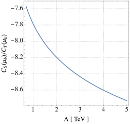
where γS=8subscript𝛾𝑆8\gamma_{S}=-8, γT=8/3subscript𝛾𝑇83\gamma_{T}=8/3 and β0(nf)=112nf/3superscriptsubscript𝛽0subscript𝑛𝑓112subscript𝑛𝑓3\beta_{0}^{(n_{f})}=11-2n_{f}/3 Dorsner:2013tla . We use the Mathematica package RunDec Chetyrkin:2000yt to run αssubscript𝛼𝑠\alpha_{s} from ΛTeVsimilar-toΛTeV\Lambda\sim\text{TeV} to μb=mb¯=4.2 GeVsubscript𝜇𝑏¯subscript𝑚𝑏4.2 GeV\mu_{b}=\overline{m_{b}}=4.2\text{ GeV}. This results in a modification of the relation between the scalar and tensor Wilson coefficients: CT(Λ)=14CS(Λ)subscript𝐶𝑇Λ14subscript𝐶𝑆ΛC_{T}(\Lambda)=-\frac{1}{4}C_{S}(\Lambda). Although most of the running occurs at the low scale (between μbsubscript𝜇𝑏\mu_{b} and mtsubscript𝑚𝑡m_{t}), the relationship between these coefficients still depends non-negligibly on the chosen high scale. To illustrate this dependence, we plot the ratio CS(μb)/CT(μb)subscript𝐶𝑆subscript𝜇𝑏subscript𝐶𝑇subscript𝜇𝑏C_{S}(\mu_{b})/C_{T}(\mu_{b}) against ΛΛ\Lambda in Fig. 1. Running down to μbsubscript𝜇𝑏\mu_{b} from higher scales increases the magnitude of the scalar coefficient relative to the tensor one.
Refer to caption
Figure 1: The dependence of the ratio of the tensor and scalar Wilson coefficients evaluated at μbsubscript𝜇𝑏\mu_{b} in bcν𝑏𝑐𝜈b\to c\ell\nu as a function of the new-physics scale ΛΛ\Lambda, at which the ratio is 44-4. The figure depicts the values down to which the ratio CS/CTsubscript𝐶𝑆subscript𝐶𝑇C_{S}/C_{T} evolves at μbsubscript𝜇𝑏\mu_{b}. For example, running from 1 TeV1 TeV1\text{ TeV} to μbsubscript𝜇𝑏\mu_{b} implies CS/CT=7.8subscript𝐶𝑆subscript𝐶𝑇7.8C_{S}/C_{T}=-7.8.

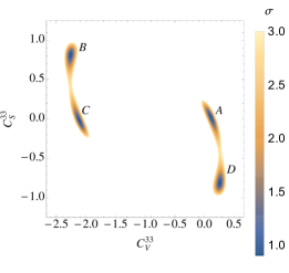
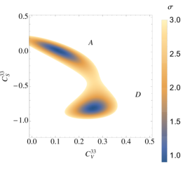
In Fig. 2 we present the results of our χ2superscript𝜒2\chi^{2} fit to the measured values of RDsubscript𝑅𝐷R_{D} and RDsubscript𝑅superscript𝐷R_{D^{*}} in CV33subscriptsuperscript𝐶33𝑉C^{33}_{V}CS33subscriptsuperscript𝐶33𝑆C^{33}_{S} space to elucidate the regions of interest. Our fit includes experimental uncertainties, but none from the theory side. We fit to our own experimental average: 0.311±0.016plus-or-minus0.3110.0160.311\pm 0.016 (an error-weighted mean calculated by adding statistical and systematic uncertainties in quadrature) which includes the most recent Belle measurements. For simplicity we assume that the phase of the operators is aligned with the SM contribution and we do not account for the experimental correlation between the measurements of RDsubscript𝑅𝐷R_{D} and RDsubscript𝑅superscript𝐷R_{D^{*}}. There exist four regions which provide a good fit to the data for Λ=1 TeVΛ1 TeV\Lambda=1\text{ TeV}, the most easily accessible has best-fit point (CV33,CS33)(0.11,0.034)superscriptsubscript𝐶𝑉33superscriptsubscript𝐶𝑆330.110.034(C_{V}^{33},C_{S}^{33})\approx(0.11,0.034), corresponding to the same region as that surrounding the point given in Eq. (13). Our results in this region are thus in good agreement with those of Ref. Freytsis:2015qca . The best-fit points of the four regions are summarized in Table 2.

Region best-fit point (CV33superscriptsubscript𝐶𝑉33C_{V}^{33}, CS33superscriptsubscript𝐶𝑆33C_{S}^{33})
A (0.11,0.034)0.110.034(0.11,0.034)
B (2.25,0.81)2.250.81(-2.25,0.81)
C (2.12,0.015)2.120.015(-2.12,-0.015)
D (0.26,0.81)0.260.81(0.26,-0.81)
Table 2: The best-fit points for our χ2superscript𝜒2\chi^{2} fit to the bcτν𝑏𝑐𝜏𝜈b\to c\tau\nu data for Λ=1 TeVΛ1 TeV\Lambda=1\text{ TeV}. Four distinct regions emerge from our analysis, of which region A𝐴A is the most convenient to attain in a UV complete model, since it involves small values of the Wilson coefficients and guarantees perturbative Yukawa couplings.
Refer to caption
Refer to caption
Figure 2: The values for CV33superscriptsubscript𝐶𝑉33C_{V}^{33} and CS33superscriptsubscript𝐶𝑆33C_{S}^{33} corresponding to a good fit to the RDsubscript𝑅𝐷R_{D} and RDsubscript𝑅superscript𝐷R_{D^{*}} data at Λ=1 TeVΛ1 TeV\Lambda=1\text{ TeV}. The colors indicate the σ𝜎\sigma values of our fit. The right plot is zoomed to the area around regions A𝐴A and D𝐷D.

3.1.2 Neutral current processes

The physics underlying the neutral current bs𝑏𝑠b\rightarrow s transitions in the model can be described by the effective Lagrangian NCsubscriptNC\mathscr{L}_{\text{NC}}:

NC=4GF2VtbVtsα4πIJCIJμ𝒪IJμ,subscriptNC4subscript𝐺𝐹2subscript𝑉𝑡𝑏subscriptsuperscript𝑉𝑡𝑠𝛼4𝜋subscript𝐼𝐽subscriptsuperscript𝐶𝜇𝐼𝐽subscriptsuperscript𝒪𝜇𝐼𝐽\mathscr{L}_{\text{NC}}=\frac{4G_{F}}{\sqrt{2}}V_{tb}V^{*}_{ts}\frac{\alpha}{4\pi}\sum_{IJ}C^{\mu}_{IJ}\mathscr{O}^{\mu}_{IJ}, (15)

where I,J{L,R}𝐼𝐽𝐿𝑅I,J\in\{L,R\} and the operators in this chiral basis are defined below in terms of 𝒪9,10subscript𝒪910\mathscr{O}_{9,10}. Following the matching procedure performed in Ref. Misiak:1992bc , we find that the field ϕitalic-ϕ\phi generates the operators

𝒪LLμ12(𝒪9μ𝒪10μ)=(s¯γμPLb)(μ¯γμPLμ),𝒪LRμ12(𝒪9μ+𝒪10μ)=(s¯γμPLb)(μ¯γμPRμ)formulae-sequencesuperscriptsubscript𝒪𝐿𝐿𝜇12superscriptsubscript𝒪9𝜇superscriptsubscript𝒪10𝜇¯𝑠superscript𝛾𝜇subscript𝑃𝐿𝑏¯𝜇subscript𝛾𝜇subscript𝑃𝐿𝜇superscriptsubscript𝒪𝐿𝑅𝜇12superscriptsubscript𝒪9𝜇superscriptsubscript𝒪10𝜇¯𝑠superscript𝛾𝜇subscript𝑃𝐿𝑏¯𝜇subscript𝛾𝜇subscript𝑃𝑅𝜇\begin{split}\mathscr{O}_{LL}^{\mu}\equiv\frac{1}{2}(\mathscr{O}_{9}^{\mu}-\mathscr{O}_{10}^{\mu})&=(\bar{s}\gamma^{\mu}P_{L}b)(\bar{\mu}\gamma_{\mu}P_{L}\mu),\\ \mathscr{O}_{LR}^{\mu}\equiv\frac{1}{2}(\mathscr{O}_{9}^{\mu}+\mathscr{O}_{10}^{\mu})&=(\bar{s}\gamma^{\mu}P_{L}b)(\bar{\mu}\gamma_{\mu}P_{R}\mu)\end{split} (16)

at the one-loop level with coefficients Bauer:2015knc

CLLϕ,μsuperscriptsubscript𝐶𝐿𝐿italic-ϕ𝜇\displaystyle C_{LL}^{\phi,\mu} =mt28παmϕ2|z23|2264παGFmϕ2VtbVtsixi3xi2j|z2j|2,absentsuperscriptsubscript𝑚𝑡28𝜋𝛼superscriptsubscript𝑚italic-ϕ2superscriptsubscript𝑧232264𝜋𝛼subscript𝐺𝐹superscriptsubscript𝑚italic-ϕ2subscript𝑉𝑡𝑏subscriptsuperscript𝑉𝑡𝑠subscript𝑖subscript𝑥𝑖3superscriptsubscript𝑥𝑖2subscript𝑗superscriptsubscript𝑧2𝑗2\displaystyle=\frac{m_{t}^{2}}{8\pi\alpha m_{\phi}^{2}}|z_{23}|^{2}-\frac{\sqrt{2}}{64\pi\alpha G_{F}m_{\phi}^{2}V_{tb}V^{*}_{ts}}\sum_{i}x_{i3}x_{i2}^{*}\sum_{j}|z_{2j}|^{2}, (17a)
CLRϕ,μ=mt216παmϕ2|y23|2[lnmϕ2mt2f(mt2mW2)]264παGFmϕ2VtbVtsixi3xi2j|y2j|2,superscriptsubscript𝐶𝐿𝑅italic-ϕ𝜇superscriptsubscript𝑚𝑡216𝜋𝛼superscriptsubscript𝑚italic-ϕ2superscriptsubscript𝑦232delimited-[]superscriptsubscript𝑚italic-ϕ2superscriptsubscript𝑚𝑡2𝑓superscriptsubscript𝑚𝑡2superscriptsubscript𝑚𝑊2264𝜋𝛼subscript𝐺𝐹superscriptsubscript𝑚italic-ϕ2subscript𝑉𝑡𝑏subscriptsuperscript𝑉𝑡𝑠subscript𝑖subscript𝑥𝑖3superscriptsubscript𝑥𝑖2subscript𝑗superscriptsubscript𝑦2𝑗2\displaystyle\begin{split}C_{LR}^{\phi,\mu}&=\frac{m_{t}^{2}}{16\pi\alpha m_{\phi}^{2}}|y_{23}|^{2}\left[\ln\frac{m_{\phi}^{2}}{m_{t}^{2}}-f\left(\frac{m_{t}^{2}}{m_{W}^{2}}\right)\right]\\ &\quad-\frac{\sqrt{2}}{64\pi\alpha G_{F}m_{\phi}^{2}V_{tb}V^{*}_{ts}}\sum_{i}x_{i3}x_{i2}^{*}\sum_{j}|y_{2j}|^{2},\end{split} (17b)

where

f(x)=13x1+3(x1)2lnx.𝑓𝑥13𝑥13superscript𝑥12𝑥f(x)=1-\frac{3}{x-1}+\frac{3}{(x-1)^{2}}\ln x. (18)

For the rest of the discussion we remove the μ𝜇\mu superscript from the Wilson coefficients and operators associated with bsμμ𝑏𝑠𝜇𝜇b\to s\mu\mu, since we only consider new-physics effects in the muonic mode. The dominant contributions are from the box diagrams shown in Fig. 3. There are additional lepton flavor universal contributions from γ𝛾\gamma and Z𝑍Z penguins, however these are subdominant: the Z𝑍Z penguins are suppressed by small neutrino masses and only the small short-range contribution from the γ𝛾\gamma penguins contributes to C9ϕsubscriptsuperscript𝐶italic-ϕ9C^{\phi}_{9}.

Refer to caption
Refer to caption
Figure 3: The box diagrams contributing to CLLϕsuperscriptsubscript𝐶𝐿𝐿italic-ϕC_{LL}^{\phi} and CLRϕsuperscriptsubscript𝐶𝐿𝑅italic-ϕC_{LR}^{\phi} in this scalar leptoquark model.
Refer to caption
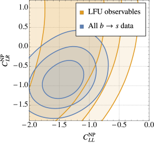
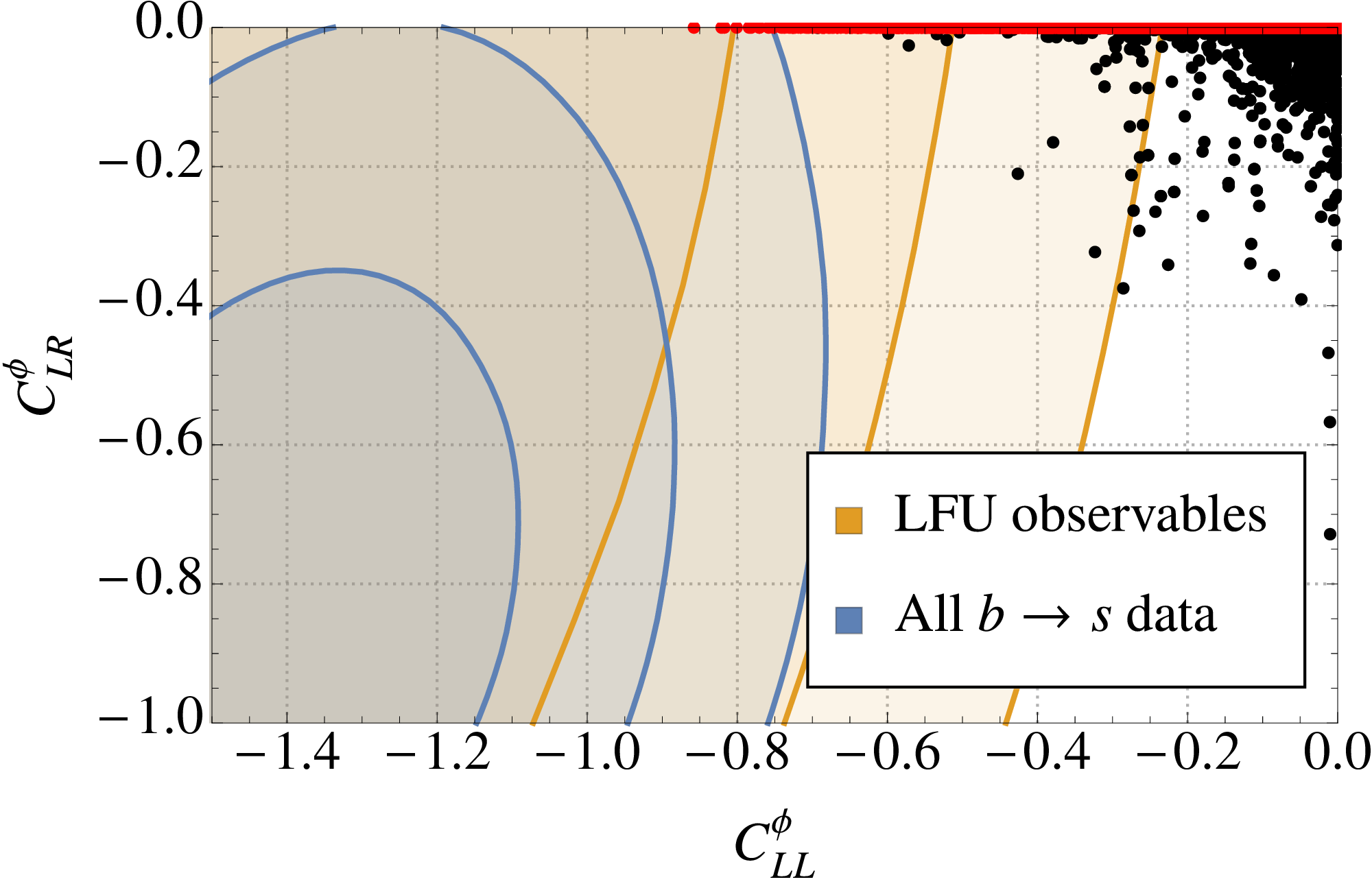
Figure 4: Fig. 1 in Ref. Altmannshofer:2017yso translated into the chiral basis. The figure shows the allowed 111, 222 and 3σ3𝜎3\sigma contours in the CLLNPsuperscriptsubscript𝐶𝐿𝐿NPC_{LL}^{\text{NP}}CLRNPsuperscriptsubscript𝐶𝐿𝑅NPC_{LR}^{\text{NP}} plane. The orange contours represent the fit to only LFU observables while the blue contours take into account all bs𝑏𝑠b\to s observables including the branching ratios of Bsμ+μsubscript𝐵𝑠superscript𝜇superscript𝜇B_{s}\to\mu^{+}\mu^{-} and the BaBar measurement of BXse+e𝐵subscript𝑋𝑠superscript𝑒superscript𝑒B\to X_{s}e^{+}e^{-} Lees:2013nxa .

The authors of Refs. Altmannshofer:2017yso ; Capdevila:2017bsm ; Ciuchini:2017mik ; Geng:2017svp ; DAmico:2017mtc conduct a global fit of all available experimental data on the bs𝑏𝑠b\rightarrow s decays. They find a good fit to the data for the chiral coefficients generated by the leptoquark for

CLLNP1.2 and CIJNP0 otherwise,superscriptsubscript𝐶𝐿𝐿NP1.2 and superscriptsubscript𝐶𝐼𝐽NP0 otherwiseC_{LL}^{\text{NP}}\approx-1.2\ \text{ and }\ C_{IJ}^{\text{NP}}\approx 0\ \text{ otherwise}, (19)

where new physics is assumed to significantly alter only the muonic mode and the fit is performed for CIJsubscript𝐶𝐼𝐽C_{IJ}\in\mathbb{R}. This choice of coefficients eliminates the tensions in RK()subscript𝑅superscript𝐾R_{K^{(*)}} and results in a significantly improved fit to all of the bs𝑏𝑠b\to s data, with a total 4.2σ4.2𝜎4.2\sigma pull from the SM Altmannshofer:2017yso . Although a better fit to all of the data can be achieved for CLRNP<0superscriptsubscript𝐶𝐿𝑅NP0C_{LR}^{\text{NP}}<0, the choice CLRNP0superscriptsubscript𝐶𝐿𝑅NP0C_{LR}^{\text{NP}}\approx 0 allows slightly smaller values of CLLNPsuperscriptsubscript𝐶𝐿𝐿NPC_{LL}^{\text{NP}} to explain the RK()subscript𝑅superscript𝐾R_{K^{(*)}} anomalies. We translate the top plot of Fig. 1 in Ref. Altmannshofer:2017yso into the chiral basis relevant for our leptoquark in Fig. 4 to elucidate the regions of interest. A good fit to the measurements of the LFU observables RKsubscript𝑅𝐾R_{K} and RKsubscript𝑅superscript𝐾R_{K^{*}} is implied for 1.8CLLϕ0.8less-than-or-similar-to1.8superscriptsubscript𝐶𝐿𝐿italic-ϕless-than-or-similar-to0.8-1.8\lesssim C_{LL}^{\phi}\lesssim-0.8 with CLRϕ=0superscriptsubscript𝐶𝐿𝑅italic-ϕ0C_{LR}^{\phi}=0 and values close to unity for the mixed-chirality contribution require smaller values for CLLϕsuperscriptsubscript𝐶𝐿𝐿italic-ϕC_{LL}^{\phi} to meet the central value of the LFU measurements. The condition CLRϕ0superscriptsubscript𝐶𝐿𝑅italic-ϕ0C_{LR}^{\phi}\approx 0 implies a suppression of the Yukawa couplings y2isubscript𝑦2𝑖y_{2i}, while CLLϕ1.2superscriptsubscript𝐶𝐿𝐿italic-ϕ1.2C_{LL}^{\phi}\approx-1.2 requires large leptoquark couplings to the second and third generation of left-handed quarks for the second term in Eq. (17a)—corresponding to the second diagram in Fig. 3—to dominate over the first, since it alone can be negative.

Throughout the text, we follow Ref. Becirevic:2016oho for the calculation of RKsubscript𝑅𝐾R_{K}.

3.1.3 Anomalous magnetic moment of the muon

The leptoquark also mediates one-loop corrections to the γμμ𝛾𝜇𝜇\gamma\mu\mu vertex, contributing to the muon anomalous magnetic moment. In the limit that mϕ2mt2much-greater-thansuperscriptsubscript𝑚italic-ϕ2superscriptsubscript𝑚𝑡2m_{\phi}^{2}\gg m_{t}^{2}, the contribution of ϕitalic-ϕ\phi to aμ=(g2)μ/2subscript𝑎𝜇subscript𝑔2𝜇2a_{\mu}=(g-2)_{\mu}/2 is given by Bauer:2015knc ; Djouadi:1989md ; Chakraverty:2001yg ; Cheung:2001ip

aμϕ=imμmui4π2mϕ2(74lnmϕ2mui2)Re(y2iz2i)mμ232π2mϕ2[i|z2i|2+i|y2i|2],superscriptsubscript𝑎𝜇italic-ϕsubscript𝑖subscript𝑚𝜇subscript𝑚subscript𝑢𝑖4superscript𝜋2superscriptsubscript𝑚italic-ϕ274superscriptsubscript𝑚italic-ϕ2superscriptsubscript𝑚subscript𝑢𝑖2Resubscript𝑦2𝑖subscript𝑧2𝑖superscriptsubscript𝑚𝜇232superscript𝜋2superscriptsubscript𝑚italic-ϕ2delimited-[]subscript𝑖superscriptsubscript𝑧2𝑖2subscript𝑖superscriptsubscript𝑦2𝑖2a_{\mu}^{\phi}=\sum_{i}\frac{m_{\mu}m_{u_{i}}}{4\pi^{2}m_{\phi}^{2}}\left(\frac{7}{4}-\ln\frac{m_{\phi}^{2}}{m_{u_{i}}^{2}}\right)\text{Re}(y_{2i}z_{2i})-\frac{m_{\mu}^{2}}{32\pi^{2}m_{\phi}^{2}}\left[\sum_{i}|z_{2i}|^{2}+\sum_{i}|y_{2i}|^{2}\right], (20)

and the same-chirality terms are suppressed relative to the mixed-chirality term by a factor of the muon mass, leading to the requirement of non-vanishing right-handed couplings for an adequate explanation. We require that the leptoquark contribution account for the measured anomaly, and thus that aμϕ=(287±80)1011superscriptsubscript𝑎𝜇italic-ϕplus-or-minus28780superscript1011a_{\mu}^{\phi}=(287\pm 80)\cdot 10^{-11} Davier:2010nc .

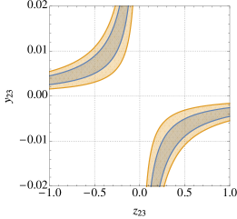
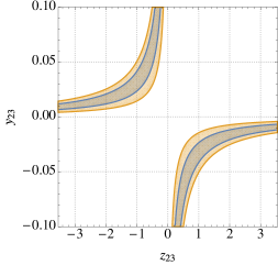
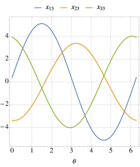
The top-mass enhancement in the first term makes this the dominant contribution in this model, and we illustrate the interesting values of y32subscript𝑦32y_{32} and z32subscript𝑧32z_{32} in Fig. 5 for leptoquark mass values of mϕ=1 TeVsubscript𝑚italic-ϕ1 TeVm_{\phi}=1\text{ TeV} and mϕ=5 TeVsubscript𝑚italic-ϕ5 TeVm_{\phi}=5\text{ TeV}. Large z23subscript𝑧23z_{23} values assist the model’s explanation of RK()subscript𝑅superscript𝐾R_{K^{(*)}}, hence a combined explanation of this and the (g2)μsubscript𝑔2𝜇(g-2)_{\mu} anomaly prefers a small y23subscript𝑦23y_{23}. Explicitly, the condition Bauer:2015knc

20.7(1+1.06lnm^ϕ)Re(y23z23)0.08m^ϕ220.711.06subscript^𝑚italic-ϕResubscript𝑦23subscript𝑧230.08superscriptsubscript^𝑚italic-ϕ2-20.7(1+1.06\ln\hat{m}_{\phi})\text{Re}(y_{23}z_{23})\approx 0.08\hat{m}_{\phi}^{2} (21)

must be satisfied to meet the central value of the measurements of aμsubscript𝑎𝜇a_{\mu} in this minimal case.

Refer to caption\phantomsubcaption
Figure 5: The 111 and 2σ2𝜎2\sigma allowed regions for aμsubscript𝑎𝜇a_{\mu} in the y23subscript𝑦23y_{23}z23subscript𝑧23z_{23} plane for leptoquark masses of mϕ=1 TeVsubscript𝑚italic-ϕ1 TeVm_{\phi}=1\text{ TeV} (left) and mϕ=5 TeVsubscript𝑚italic-ϕ5 TeVm_{\phi}=5\text{ TeV} (right). The top-mass enhancement in the first term of Eq. (20) allows the model to accommodate aμsubscript𝑎𝜇a_{\mu} with very small values for |y23|subscript𝑦23|y_{23}| with z230subscript𝑧230z_{23}\neq 0.

3.2 Constraints

We proceed by studying the constraints important for the leptoquark ϕitalic-ϕ\phi in the regions of parameter space dictated by the flavor anomalies. This analysis includes the constraints imposed by B𝐵B, K𝐾K and D𝐷D meson decays, Bssubscript𝐵𝑠B_{s}B¯ssubscript¯𝐵𝑠\bar{B}_{s} mixing, lepton-flavor violating processes and electroweak measurements.

Many of these processes are studied in the context of an effective-operator framework. Since much of the nomenclature for four-fermion operator coefficients is often only based on the Lorentz-structure of each term, keeping the naming conventions present in the flavor-physics literature for each process can lead to ambiguity. For this reason we index each effective Lagrangian appearing in this section and retain the common names for each term, with the Lagrangian’s index prepended to the label. For example, Ci,VLsubscript𝐶𝑖subscript𝑉𝐿C_{i,V_{L}} might correspond to the coefficient of an operator like (ϕ¯γμPLχ)(ψ¯γμPLω)¯italic-ϕsubscript𝛾𝜇subscript𝑃𝐿𝜒¯𝜓superscript𝛾𝜇subscript𝑃𝐿𝜔(\bar{\phi}\gamma_{\mu}P_{L}\chi)(\bar{\psi}\gamma^{\mu}P_{L}\omega) in isubscript𝑖\mathscr{L}_{i}, where ϕ,χ,ψ,ωitalic-ϕ𝜒𝜓𝜔\phi,\chi,\psi,\omega represent Fermion fields. For clarity we remind the reader that the coefficients of CCsubscriptCC\mathscr{L}_{\textsc{CC}} and NCsubscriptNC\mathscr{L}_{\textsc{NC}} from the previous section are left unindexed.

For the reader’s convenience, we signpost the important results of this section below.

Constraints on the left-handed couplings.

A feature of the BN model is that the effective operators mediating the bsμμ𝑏𝑠𝜇𝜇b\to s\mu\mu decays are generated through box diagrams, since ϕitalic-ϕ\phi only couples down-type quarks to neutrinos at tree-level. As a consequence, the large Yukawa couplings required to meet the bs𝑏𝑠b\to s measurements will mediate FCNC processes with a neutrino pair in the final state—processes to which they are related by SU(2)LSUsubscript2𝐿\textrm{SU}(2)_{L} invariance—at tree level. This makes the bsνν𝑏𝑠𝜈𝜈b\to s\nu\nu decays and K+π+ννsuperscript𝐾superscript𝜋𝜈𝜈K^{+}\to\pi^{+}\nu\nu very constraining for this model’s explanation of RK()subscript𝑅superscript𝐾R_{K^{(*)}}. The former decay is more important, since it involves the combination of left-handed couplings present in Eq. (17): ixi3xi2subscript𝑖subscript𝑥𝑖3subscriptsuperscript𝑥𝑖2\sum_{i}x_{i3}x^{*}_{i2}, and essential to ensure a negative value for CLLϕsubscriptsuperscript𝐶italic-ϕ𝐿𝐿C^{\phi}_{LL}. The leptoquark also contributes to Bssubscript𝐵𝑠B_{s}B¯ssubscript¯𝐵𝑠\bar{B}_{s} mixing through box diagrams similar to those given in Fig. 3 with neutrinos running through both internal fermion lines. We find measurements of Bssubscript𝐵𝑠B_{s}B¯ssubscript¯𝐵𝑠\bar{B}_{s} mixing to be more constraining than those of FCNC decays for leptoquark masses larger than a few TeV. For small leptoquark masses, precision electroweak measurements of the Z¯𝑍¯Z\ell\bar{\ell} couplings place upper bounds on the sum of the absolute squares of left-handed couplings, and a relative sign difference between couplings to the third-generation quarks and those to the second implies the possibility of a mild cancellation taming these effects. A very important constraint on the left-handed coupling |x22|subscript𝑥22|x_{22}| can be derived from the meson decay D0μμsuperscript𝐷0𝜇𝜇D^{0}\to\mu\mu, a large value of which aids the explanation of RK()subscript𝑅superscript𝐾R_{K^{(*)}} in this scenario. It has also recently been pointed out Becirevic:2016oho that the LFU evident in the ratio RDμ/e=Γ(B¯Dμν¯)/Γ(B¯Deν¯)superscriptsubscript𝑅𝐷𝜇𝑒Γ¯𝐵𝐷𝜇¯𝜈Γ¯𝐵𝐷𝑒¯𝜈R_{D}^{\mu/e}=\Gamma(\bar{B}\rightarrow D\mu\bar{\nu})/\Gamma(\bar{B}\rightarrow De\bar{\nu}) represents a significant hurdle to the leptoquark’s explanation of RKsubscript𝑅𝐾R_{K}, and we discuss this constraint below.

Constraints on the product of left-handed couplings discussed above also frustrate the model’s attempts to explain measurements of the ratios RDsubscript𝑅𝐷R_{D} and RDsubscript𝑅superscript𝐷R_{D^{*}}, specifically in those areas of parameter space suggested by new-physics effects only in CVijsuperscriptsubscript𝐶𝑉𝑖𝑗C_{V}^{ij}. This implies the need for non-vanishing right-handed couplings yijsubscript𝑦𝑖𝑗y_{ij}.

Constraints on the right-handed couplings.

The right-handed couplings yijsubscript𝑦𝑖𝑗y_{ij} are generally less constrained in this leptoquark model, since they mediate interactions involving fewer fermion species. The most stringent limits come from mixed-chirality contributions to tau decays such as τμμμ𝜏𝜇𝜇𝜇\tau\to\mu\mu\mu and τμγ𝜏𝜇𝛾\tau\to\mu\gamma, as well as the precision electroweak measurements mentioned above. Many right-handed couplings also feature in the model’s contributions to B𝐵B, D𝐷D, and K𝐾K decays.

3.2.1 Semileptonic charged current processes

Leptonic and semileptonic charged current processes are a sensitive probe of the model we study, since the leptoquark ϕitalic-ϕ\phi provides tree-level channels for leptonic pseudoscalar meson decays and semileptonic decays of the tau. In order to describe these processes, we generalize the Lagrangian presented in Eq. (11) to

1ijkl=4GF2Vuidj[C1,Vijkl(u¯iγμPLdj)(¯kγμPLνl)+C1,Sijkl(u¯iPLdj)(¯kPLνl)+C1,Tijkl(u¯iσμνPLdj)(¯kσμνPLνl)],subscriptsuperscript𝑖𝑗𝑘𝑙14subscript𝐺𝐹2subscript𝑉subscript𝑢𝑖subscript𝑑𝑗delimited-[]superscriptsubscript𝐶1𝑉𝑖𝑗𝑘𝑙subscript¯𝑢𝑖superscript𝛾𝜇subscript𝑃𝐿subscript𝑑𝑗subscript¯𝑘subscript𝛾𝜇subscript𝑃𝐿subscript𝜈𝑙subscriptsuperscript𝐶𝑖𝑗𝑘𝑙1𝑆subscript¯𝑢𝑖subscript𝑃𝐿subscript𝑑𝑗subscript¯𝑘subscript𝑃𝐿subscript𝜈𝑙subscriptsuperscript𝐶𝑖𝑗𝑘𝑙1𝑇subscript¯𝑢𝑖superscript𝜎𝜇𝜈subscript𝑃𝐿subscript𝑑𝑗subscript¯𝑘subscript𝜎𝜇𝜈subscript𝑃𝐿subscript𝜈𝑙\begin{split}\mathscr{L}^{ijkl}_{1}&=-\frac{4G_{F}}{\sqrt{2}}V_{u_{i}d_{j}}\left[C_{1,V}^{ijkl}(\bar{u}_{i}\gamma^{\mu}P_{L}d_{j})(\bar{\ell}_{k}\gamma_{\mu}P_{L}\nu_{l})+C^{ijkl}_{1,S}(\bar{u}_{i}P_{L}d_{j})(\bar{\ell}_{k}P_{L}\nu_{l})\right.\\ &\quad\left.+C^{ijkl}_{1,T}(\bar{u}_{i}\sigma^{\mu\nu}P_{L}d_{j})(\bar{\ell}_{k}\sigma_{\mu\nu}P_{L}\nu_{l})\right],\end{split} (22)

where the vector, scalar and tensor Wilson coefficients at the leptoquark mass scale now read

C1,Vijklsuperscriptsubscript𝐶1𝑉𝑖𝑗𝑘𝑙\displaystyle C_{1,V}^{ijkl} =122GFVuidjzkjxli2mϕ2+δkl,absent122subscript𝐺𝐹subscript𝑉subscript𝑢𝑖subscript𝑑𝑗superscriptsubscript𝑧𝑘𝑗subscript𝑥𝑙𝑖2superscriptsubscript𝑚italic-ϕ2subscript𝛿𝑘𝑙\displaystyle=\frac{1}{2\sqrt{2}G_{F}V_{u_{i}d_{j}}}\frac{z_{kj}^{*}x_{li}}{2m_{\phi}^{2}}+\delta_{kl}, (23a)
C1,Sijklsuperscriptsubscript𝐶1𝑆𝑖𝑗𝑘𝑙\displaystyle C_{1,S}^{ijkl} =122GFVuidjykjxli2mϕ2,absent122subscript𝐺𝐹subscript𝑉subscript𝑢𝑖subscript𝑑𝑗subscript𝑦𝑘𝑗subscript𝑥𝑙𝑖2superscriptsubscript𝑚italic-ϕ2\displaystyle=\frac{1}{2\sqrt{2}G_{F}V_{u_{i}d_{j}}}\frac{y_{kj}x_{li}}{2m_{\phi}^{2}}, (23b)
C1,Tijklsuperscriptsubscript𝐶1𝑇𝑖𝑗𝑘𝑙\displaystyle C_{1,T}^{ijkl} =14C1,Sijkl,absent14superscriptsubscript𝐶1𝑆𝑖𝑗𝑘𝑙\displaystyle=-\frac{1}{4}C_{1,S}^{ijkl}, (23c)

in analogy with Eqs. (12). The leptonic decay rate for a pseudoscalar meson Piju¯idjsimilar-tosubscript𝑃𝑖𝑗subscript¯𝑢𝑖subscript𝑑𝑗P_{ij}\sim\bar{u}_{i}d_{j} is then given by Becirevic:2016oho

Γ(Pijkνl)=GF2mP|Vuidj|28πfP2mk2(1ml2mP2)2|C1,VijklC1,SijklmP2mk(mui+mdj)|2,Γsubscript𝑃𝑖𝑗subscript𝑘subscript𝜈𝑙superscriptsubscript𝐺𝐹2subscript𝑚𝑃superscriptsubscript𝑉subscript𝑢𝑖subscript𝑑𝑗28𝜋superscriptsubscript𝑓𝑃2superscriptsubscript𝑚subscript𝑘2superscript1superscriptsubscript𝑚subscript𝑙2superscriptsubscript𝑚𝑃22superscriptsuperscriptsubscript𝐶1𝑉𝑖𝑗𝑘𝑙superscriptsubscript𝐶1𝑆𝑖𝑗𝑘𝑙superscriptsubscript𝑚𝑃2subscript𝑚subscript𝑘subscript𝑚subscript𝑢𝑖subscript𝑚subscript𝑑𝑗2\begin{split}\Gamma(P_{ij}\to\ell_{k}\nu_{l})&=\frac{G_{F}^{2}m_{P}|V_{u_{i}d_{j}}|^{2}}{8\pi}f_{P}^{2}m_{\ell_{k}}^{2}\left(1-\frac{m_{\ell_{l}}^{2}}{m_{P}^{2}}\right)^{2}\\ &\quad\cdot\left|C_{1,V}^{ijkl}-C_{1,S}^{ijkl}\frac{m_{P}^{2}}{m_{\ell_{k}}(m_{u_{i}}+m_{d_{j}})}\right|^{2},\end{split} (24)

where fPsubscript𝑓𝑃f_{P} is the pseudoscalar meson decay constant. As before, we account for the effect of the running of αssubscript𝛼𝑠\alpha_{s} from the high scale to the scales appropriate for each decay for the scalar operator. We take the relevant scale to be μ=mc¯=1.27 GeV𝜇¯subscript𝑚𝑐1.27 GeV\mu=\overline{m_{c}}=1.27\text{ GeV} for the D𝐷D meson decays and μ=2 GeV𝜇2 GeV\mu=2\text{ GeV} for the K𝐾K decays, since this is the matching scale used in Ref. Aoki:2016frl , from which we take the decay constants. Explicitly,

C1,S(μ)=[αs(mb)αs(μ)]γS2β0(4)[αs(mt)αs(mb)]γS2β0(5)[αs(Λ)αs(mt)]γS2β0(6)C1,S(Λ),subscript𝐶1𝑆𝜇superscriptdelimited-[]subscript𝛼𝑠subscript𝑚𝑏subscript𝛼𝑠𝜇subscript𝛾𝑆2superscriptsubscript𝛽04superscriptdelimited-[]subscript𝛼𝑠subscript𝑚𝑡subscript𝛼𝑠subscript𝑚𝑏subscript𝛾𝑆2superscriptsubscript𝛽05superscriptdelimited-[]subscript𝛼𝑠Λsubscript𝛼𝑠subscript𝑚𝑡subscript𝛾𝑆2superscriptsubscript𝛽06subscript𝐶1𝑆ΛC_{1,S}(\mu)=\left[\frac{\alpha_{s}(m_{b})}{\alpha_{s}(\mu)}\right]^{\frac{\gamma_{S}}{2\beta_{0}^{(4)}}}\left[\frac{\alpha_{s}(m_{t})}{\alpha_{s}(m_{b})}\right]^{\frac{\gamma_{S}}{2\beta_{0}^{(5)}}}\left[\frac{\alpha_{s}(\Lambda)}{\alpha_{s}(m_{t})}\right]^{\frac{\gamma_{S}}{2\beta_{0}^{(6)}}}C_{1,S}(\Lambda), (25)

while the running for the scalar operator featuring in the B𝐵B decays is the same as in Eq. (14). Eq. (24) is finely sensitive to the Wilson coefficient C1,Ssubscript𝐶1𝑆C_{1,S} since it has the effect of lifting the chiral suppression of the SM due to the charged lepton mass in the denominator of the last term. Recent work Becirevic:2016oho has pointed out the importance of considering the decays Bν¯𝐵¯𝜈B\to\ell\bar{\nu}, Kν¯𝐾¯𝜈K\to\ell\bar{\nu}, Dsν¯subscript𝐷𝑠¯𝜈D_{s}\to\ell\bar{\nu} and BD()ν𝐵superscript𝐷𝜈B\to D^{(*)}\ell\nu, to which we also add a discussion of τKν𝜏𝐾𝜈\tau\to K\nu and Bcν¯subscript𝐵𝑐¯𝜈B_{c}\to\ell\bar{\nu} below. In addition, for each relevant process we calculate a LFU ratio, since in many cases these are well measured quantities which constitute powerful probes of any new-physics attempting to explain RD()subscript𝑅superscript𝐷R_{D^{(*)}} or RK()subscript𝑅superscript𝐾R_{K^{(*)}}. We summarize the limits and values we take for these decays and their relevant ratios in Table 3. All values of the decay constants used throughout this discussion are taken from Ref. Aoki:2016frl .

Observable Experimental value
Br(Kμν)Br𝐾𝜇𝜈\text{Br}(K\to\mu\nu) (63.56±0.11)%percentplus-or-minus63.560.11(63.56\pm 0.11)\%
Br(Dsμν)Brsubscript𝐷𝑠𝜇𝜈\text{Br}(D_{s}\to\mu\nu) (0.556±0.025)%percentplus-or-minus0.5560.025(0.556\pm 0.025)\%
Br(Dsτν)Brsubscript𝐷𝑠𝜏𝜈\text{Br}(D_{s}\to\tau\nu) (5.55±0.24)%percentplus-or-minus5.550.24(5.55\pm 0.24)\%
Br(Bμν)Br𝐵𝜇𝜈\text{Br}(B\to\mu\nu) <1.0106absent1.0superscript106<1.0\cdot 10^{-6}
Br(Bτν)Br𝐵𝜏𝜈\text{Br}(B\to\tau\nu) (1.09±0.24)104plus-or-minus1.090.24superscript104(1.09\pm 0.24)\cdot 10^{-4}
Br(Bcτν)Brsubscript𝐵𝑐𝜏𝜈\text{Br}(B_{c}\to\tau\nu) 30%less-than-or-similar-toabsentpercent30\lesssim 30\% Alonso:2016oyd
rKe/μ=Γ(Keν)Γ(Kμν)superscriptsubscript𝑟𝐾𝑒𝜇Γ𝐾𝑒𝜈Γ𝐾𝜇𝜈r_{K}^{e/\mu}=\frac{\Gamma(K\to e\nu)}{\Gamma(K\to\mu\nu)} (2.488±0.009)105plus-or-minus2.4880.009superscript105(2.488\pm 0.009)\cdot 10^{-5}
RKτ/μ=Γ(τKν)Γ(Kμν)superscriptsubscript𝑅𝐾𝜏𝜇Γ𝜏𝐾𝜈Γ𝐾𝜇𝜈R_{K}^{\tau/\mu}=\frac{\Gamma(\tau\to K\nu)}{\Gamma(K\to\mu\nu)} (1.101±0.016)102plus-or-minus1.1010.016superscript102(1.101\pm 0.016)\cdot 10^{-2}
RDsτ/μ=Γ(Dsτν)Γ(Dsμν)superscriptsubscript𝑅subscript𝐷𝑠𝜏𝜇Γsubscript𝐷𝑠𝜏𝜈Γsubscript𝐷𝑠𝜇𝜈R_{D_{s}}^{\tau/\mu}=\frac{\Gamma(D_{s}\to\tau\nu)}{\Gamma(D_{s}\to\mu\nu)} 10.73±0.690.53+0.56plus-or-minus10.73subscriptsuperscript0.690.560.5310.73\pm 0.69^{+0.56}_{-0.53} Zupanc:2013byn
RDμ/e=Γ(BDμν)Γ(BDeν)superscriptsubscript𝑅𝐷𝜇𝑒Γ𝐵𝐷𝜇𝜈Γ𝐵𝐷𝑒𝜈R_{D}^{\mu/e}=\frac{\Gamma(B\to D\mu\nu)}{\Gamma(B\to De\nu)} 0.995±0.022±0.039plus-or-minus0.9950.0220.0390.995\pm 0.022\pm 0.039 Glattauer:2015teq
RDe/μ=Γ(BDeν)Γ(BDμν)superscriptsubscript𝑅superscript𝐷𝑒𝜇Γ𝐵superscript𝐷𝑒𝜈Γ𝐵superscript𝐷𝜇𝜈R_{D^{*}}^{e/\mu}=\frac{\Gamma(B\to D^{*}e\nu)}{\Gamma(B\to D^{*}\mu\nu)} 1.04±0.05±0.01plus-or-minus1.040.050.011.04\pm 0.05\pm 0.01 Abdesselam:2017kjf
Table 3: A table summarizing the experimental values we take for the various leptonic branching ratios and LFU ratios considered in this section. Measurements quoted without explicit citation are taken from Ref. Olive:2016xmw .

The ratio

rKe/μ=Γ(Keν)Γ(Kμν)superscriptsubscript𝑟𝐾𝑒𝜇Γ𝐾𝑒𝜈Γ𝐾𝜇𝜈r_{K}^{e/\mu}=\frac{\Gamma(K\to e\nu)}{\Gamma(K\to\mu\nu)} (26)

is one of the most precisely measured quantities in weak hadronic physics. As such, the consideration of next-to-leading-order corrections becomes important for our phenomenological analysis of the effects of the leptoquark ϕitalic-ϕ\phi on these decays. Electroweak effects contributing to rKe/μsuperscriptsubscript𝑟𝐾𝑒𝜇r_{K}^{e/\mu} have been calculated to order e2p4superscript𝑒2superscript𝑝4e^{2}p^{4} in chiral perturbation theory, e.g. Cirigliano:2007ga ; Finkemeier:1994ev . Higher order contributions to the quotient Eq. (26) are proportional to the lowest order contribution: rKe/μ,(0)superscriptsubscript𝑟𝐾𝑒𝜇0r_{K}^{e/\mu,(0)}, calculated directly from Eq. (24). Including the effects of leading higher-order logarithms through ΔLLsubscriptΔ𝐿𝐿\Delta_{LL}, Eq. (26) can be written

rKe/μ=rKe/μ,(0)(1+Δe2p2K+Δe2p4K+)(1+ΔLL)superscriptsubscript𝑟𝐾𝑒𝜇superscriptsubscript𝑟𝐾𝑒𝜇01subscriptsuperscriptΔ𝐾superscript𝑒2superscript𝑝2subscriptsuperscriptΔ𝐾superscript𝑒2superscript𝑝41subscriptΔ𝐿𝐿r_{K}^{e/\mu}=r_{K}^{e/\mu,(0)}\left(1+\Delta^{K}_{e^{2}p^{2}}+\Delta^{K}_{e^{2}p^{4}}+\cdots\right)\left(1+\Delta_{LL}\right) (27)

and we take ΔLL=0.055%subscriptΔ𝐿𝐿percent0.055\Delta_{LL}=0.055\%, Δe2p2K=3.786%superscriptsubscriptΔsuperscript𝑒2superscript𝑝2𝐾percent3.786\Delta_{e^{2}p^{2}}^{K}=-3.786\% and Δe2p4K=(0.135±0.011)%superscriptsubscriptΔsuperscript𝑒2superscript𝑝4𝐾percentplus-or-minus0.1350.011\Delta_{e^{2}p^{4}}^{K}=(0.135\pm 0.011)\% Cirigliano:2007ga in our calculation.

One can extend the study of lepton-flavor universality in leptonic kaon decays by considering the crossed process τKν𝜏𝐾𝜈\tau\to K\nu. More specifically, the ratio

RKτ/μ=Γ(τKν)Γ(Kμν)superscriptsubscript𝑅𝐾𝜏𝜇Γ𝜏𝐾𝜈Γ𝐾𝜇𝜈R_{K}^{\tau/\mu}=\frac{\Gamma(\tau\to K\nu)}{\Gamma(K\to\mu\nu)} (28)

can be used to derive constraints on the muon and tau couplings of the leptoquark ϕitalic-ϕ\phi, and a similar approach has been taken to constrain the couplings of a vector leptoquark in Ref. Fajfer:2015ycq . For the numerator, we find

Γ(τKν)=GF2|Vus|28πfK2mτ3(1mK2mτ2)2i|C1,V123iC1,S123imK2mτ(mu+ms)|2,Γ𝜏𝐾𝜈superscriptsubscript𝐺𝐹2superscriptsubscript𝑉𝑢𝑠28𝜋superscriptsubscript𝑓𝐾2superscriptsubscript𝑚𝜏3superscript1superscriptsubscript𝑚𝐾2superscriptsubscript𝑚𝜏22subscript𝑖superscriptsuperscriptsubscript𝐶1𝑉123𝑖superscriptsubscript𝐶1𝑆123𝑖superscriptsubscript𝑚𝐾2subscript𝑚𝜏subscript𝑚𝑢subscript𝑚𝑠2\Gamma(\tau\to K\nu)=\frac{G_{F}^{2}|V_{us}|^{2}}{8\pi}f_{K}^{2}m_{\tau}^{3}\left(1-\frac{m_{K}^{2}}{m_{\tau}^{2}}\right)^{2}\sum_{i}\left|C_{1,V}^{123i}-C_{1,S}^{123i}\frac{m_{K}^{2}}{m_{\tau}(m_{u}+m_{s})}\right|^{2}, (29)

and the ratio RKτ/μsuperscriptsubscript𝑅𝐾𝜏𝜇R_{K}^{\tau/\mu} is required to lie within 2σ2𝜎2\sigma of its experimental value: (1.101±0.016)102plus-or-minus1.1010.016superscript102(1.101\pm 0.016)\cdot 10^{-2} Olive:2016xmw .

Pion leptonic decays have been well-studied in the context of leptoquark models, and measurements of the ratio Rπμ/e=Γ(πμν)/Γ(πeν)superscriptsubscript𝑅𝜋𝜇𝑒Γ𝜋𝜇𝜈Γ𝜋𝑒𝜈R_{\pi}^{\mu/e}=\Gamma(\pi\to\mu\nu)/\Gamma(\pi\to e\nu) demand that leptoquark interactions with the electron and first-generation quarks are small555In the most minimal case, a non-zero x21subscript𝑥21x_{21} implies z21x21subscript𝑧21subscript𝑥21z_{21}\approx x_{21} and these couplings alone are sufficient to mediate the decay π+μ+νsuperscript𝜋superscript𝜇𝜈\pi^{+}\rightarrow\mu^{+}\nu. Buchmuller:1986iq ; Davidson:1993qk . The electron and down-quark couplings play no role in the anomalies we consider in this work, and we only require that the appropriate couplings are small enough to evade these constraints.

Comments on lepton flavor universality in BD()(e,μ)ν¯𝐵superscript𝐷𝑒𝜇¯𝜈B\to D^{(*)}(e,\mu)\bar{\nu}.

An additional constraint comes from the observation that LFU is respected in the ratio of decay rates

RD()μ/e=Γ(B¯D()μν¯)Γ(B¯D()eν¯),superscriptsubscript𝑅superscript𝐷𝜇𝑒Γ¯𝐵superscript𝐷𝜇¯𝜈Γ¯𝐵superscript𝐷𝑒¯𝜈R_{D^{(*)}}^{\mu/e}=\frac{\Gamma(\bar{B}\rightarrow D^{(*)}\mu\bar{\nu})}{\Gamma(\bar{B}\rightarrow D^{(*)}e\bar{\nu})}, (30)

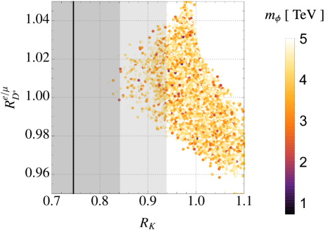
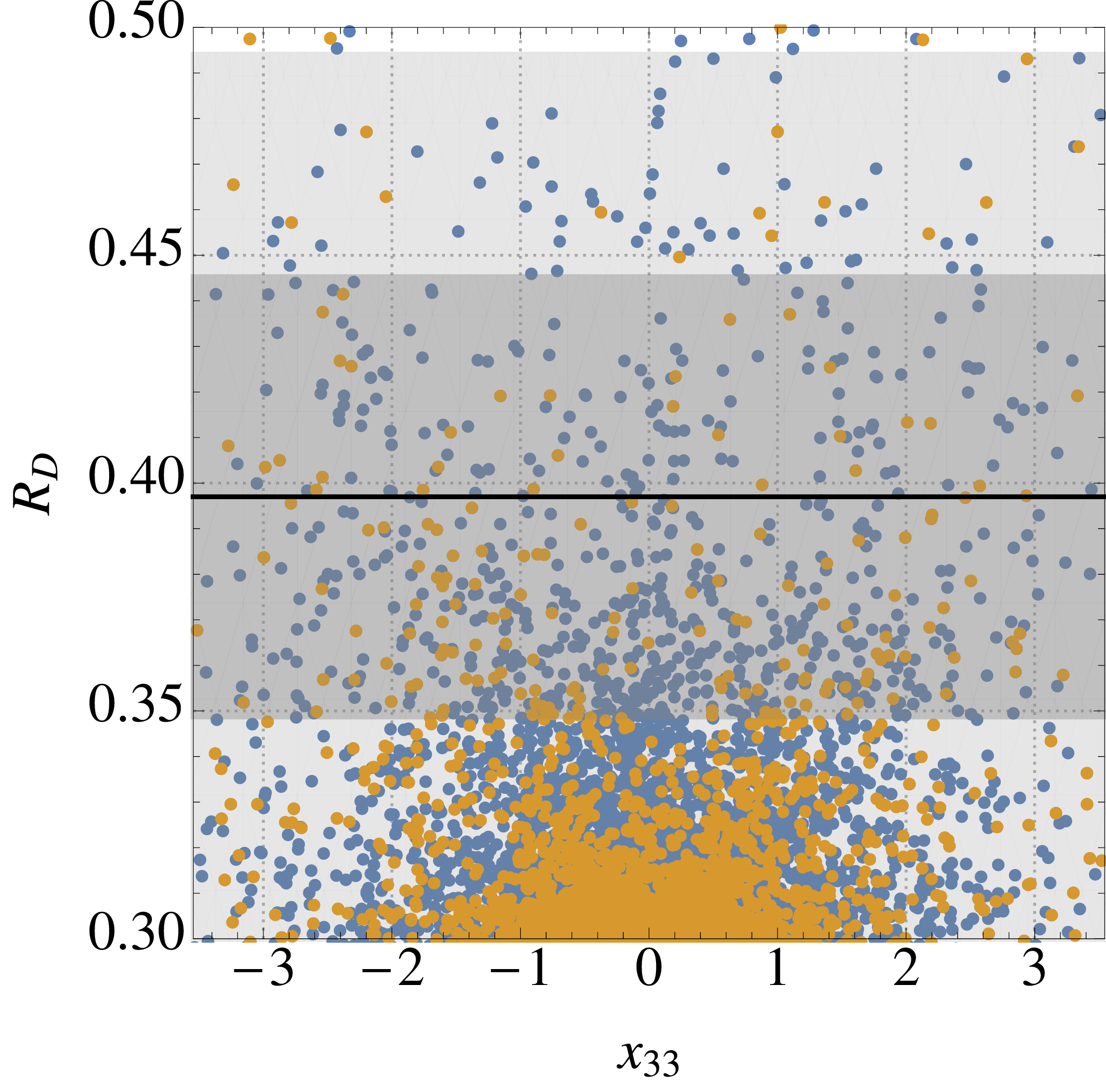
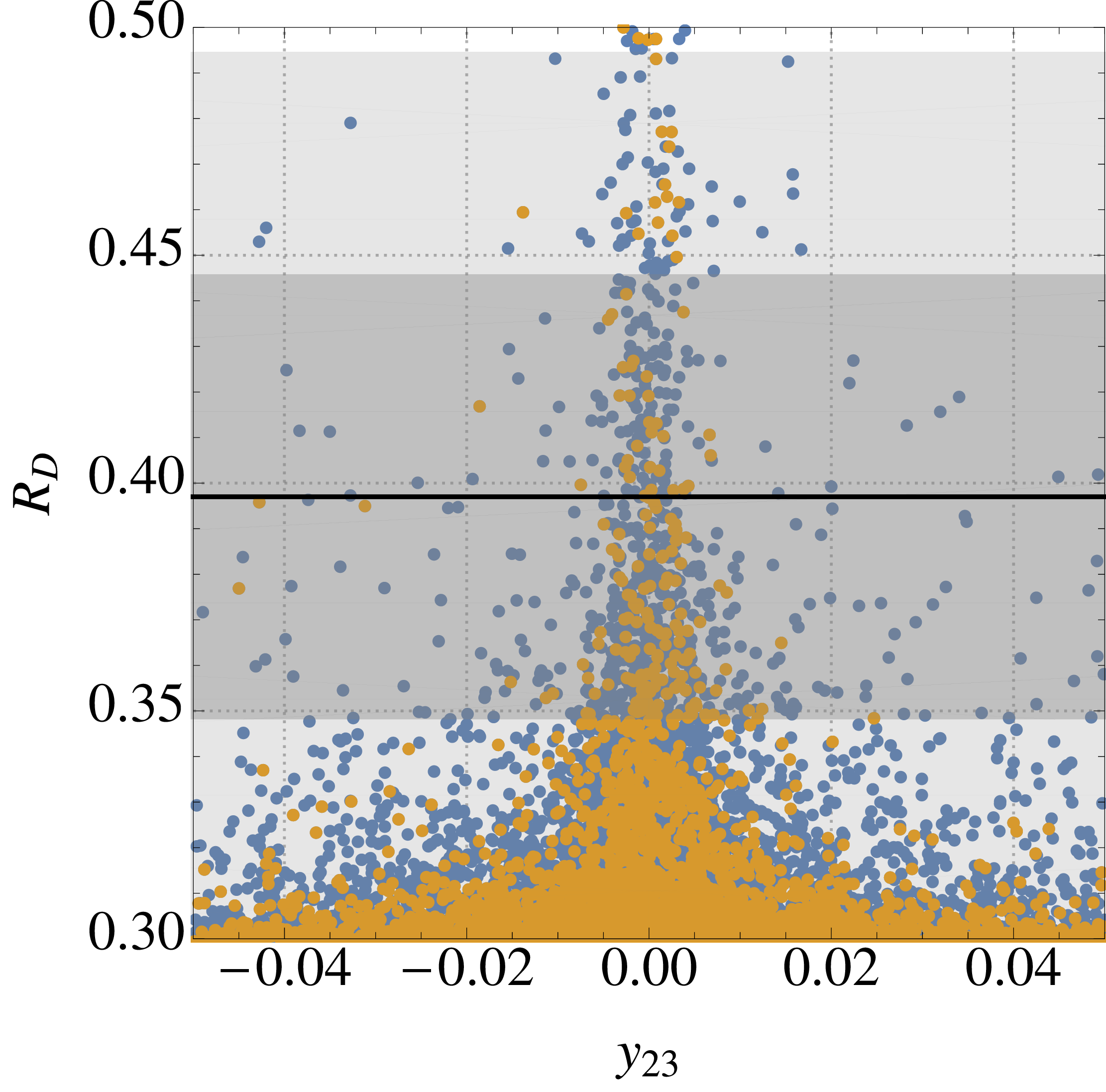
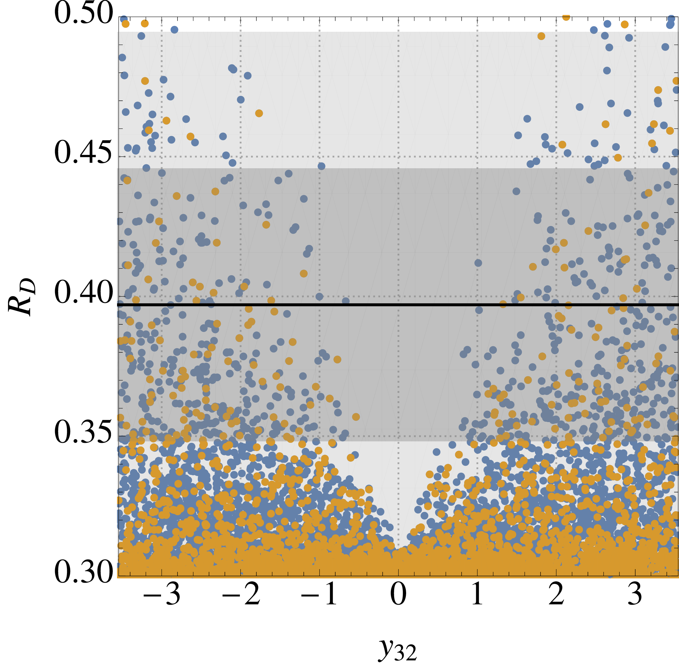
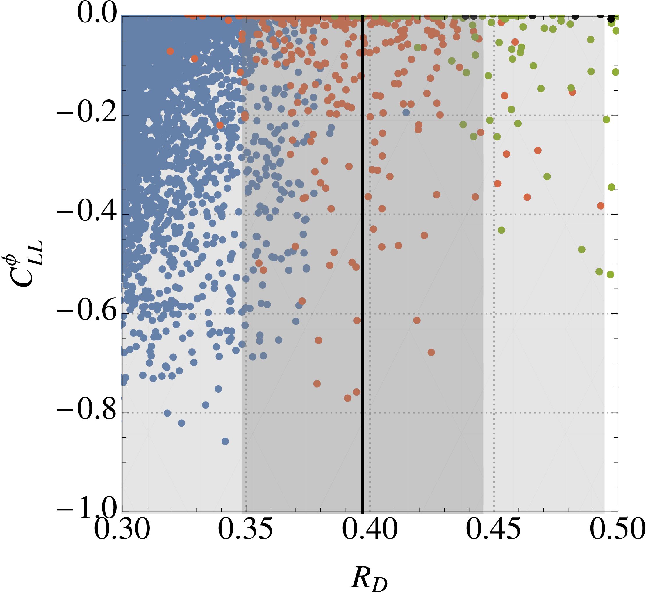
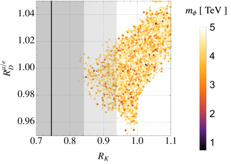
implying a tension with the purported violation in μ𝜇\mue𝑒e universality evident in RK()subscript𝑅superscript𝐾R_{K^{(*)}}. This constraint has been studied in Ref. Becirevic:2016oho , where it was concluded that the leptoquark model cannot respect this constraint while explaining the suppression of RKsubscript𝑅𝐾R_{K} in the absence of the right-handed couplings yijsubscript𝑦𝑖𝑗y_{ij}. The ratio has been measured to be RDμ/e=0.995±0.022±0.039superscriptsubscript𝑅𝐷𝜇𝑒plus-or-minus0.9950.0220.039R_{D}^{\mu/e}=0.995\pm 0.022\pm 0.039 Glattauer:2015teq , while the reciprocal is presented for the Dsuperscript𝐷D^{*} ratio: RDe/μ=1.04±0.05±0.01superscriptsubscript𝑅superscript𝐷𝑒𝜇plus-or-minus1.040.050.01R_{D^{*}}^{e/\mu}=1.04\pm 0.05\pm 0.01 Abdesselam:2017kjf . In the case of RDμ/esuperscriptsubscript𝑅𝐷𝜇𝑒R_{D}^{\mu/e}, 2σ2𝜎2\sigma consistency with the measurement allows for an approximately 10%percent1010\% deviation from the SM prediction, a weaker bound than that presented in Ref. Becirevic:2016oho , while the recent Belle result for RDe/μsuperscriptsubscript𝑅superscript𝐷𝑒𝜇R_{D^{*}}^{e/\mu} permits only a 4%percent44\% deviation for contributions to the muonic mode. We find that these constraints become less important for leptoquark masses larger than 1 TeV1 TeV1\text{ TeV}, permitting sizeable contributions to RKsubscript𝑅𝐾R_{K} in this model. We illustrate this point in the top plot of Fig. 6, where random points passing all of the constraints presented in our analysis except RDe/μsuperscriptsubscript𝑅superscript𝐷𝑒𝜇R_{D^{*}}^{e/\mu} are presented in the RKsubscript𝑅𝐾R_{K}RDμ/esuperscriptsubscript𝑅𝐷𝜇𝑒R_{D}^{\mu/e} plane. The parameters and ranges taken in our scan are the same as those of scan I in Sec. 4 in which masses are sampled randomly from the range [1,5] TeV15 TeV[1,5]\text{ TeV}. The complementary set-up for RDe/μsuperscriptsubscript𝑅superscript𝐷𝑒𝜇R_{D^{*}}^{e/\mu} is shown in the bottom figure of Fig. 6, mutatis mutandis.
Refer to caption
Refer to caption
Figure 6: The results of our random scan showing RKsubscript𝑅𝐾R_{K} against RDμ/esuperscriptsubscript𝑅𝐷𝜇𝑒R_{D}^{\mu/e} (top) and RDe/μsubscriptsuperscript𝑅𝑒𝜇superscript𝐷R^{e/\mu}_{D^{*}} (bottom) for the parameter choices detailed in Sec. 4 for ‘scan I’, in which the leptoquark mass is allowed to vary to values as large as 5 TeV5 TeV5\text{ TeV}. For leptoquark masses between 333 and 5 TeV5 TeV5\text{ TeV}, the tension in RKsubscript𝑅𝐾R_{K} can be significantly resolved while keeping LFU effects between electron and muon modes mild.
Comments on Bcτνsubscript𝐵𝑐𝜏𝜈B_{c}\to\tau\nu.

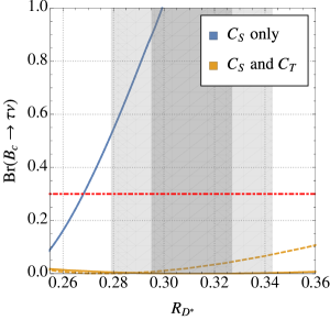
The leptonic decays of the charmed B𝐵B meson have not yet been measured—few Bcsubscript𝐵𝑐B_{c} mesons are produced at e+esuperscript𝑒superscript𝑒e^{+}e^{-} B𝐵B-factories and the leptonic mode cannot be reliably reconstructed at LHCb. Despite this, measurements of the Bcsubscript𝐵𝑐B_{c} lifetime have recently been shown to imply serious constraints Li:2016vvp ; Alonso:2016oyd for models explaining RD()subscript𝑅superscript𝐷R_{D^{(*)}} with contributions to the operator CS3isuperscriptsubscript𝐶𝑆3𝑖C_{S}^{3i} defined in Eq. (11). Here, we wish to point out that the Bcτνsubscript𝐵𝑐𝜏𝜈B_{c}\to\tau\nu rate remains SM-like in this leptoquark model due to the presence of the tensor contribution CT3isuperscriptsubscript𝐶𝑇3𝑖C_{T}^{3i}, and thus that measurements of the Bcsubscript𝐵𝑐B_{c} lifetime do not constitute a serious constraint on the model.

In Fig. 7 we plot the branching ratio Br(Bcτν)Brsubscript𝐵𝑐𝜏𝜈\text{Br}(B_{c}\to\tau\nu) in this leptoquark model against interesting values of RDsubscript𝑅superscript𝐷R_{D^{*}}, in the spirit of Fig. 1 of Ref. Alonso:2016oyd . The blue curve represents the contribution from only the Wilson coefficient CSsubscript𝐶𝑆C_{S}, while the orange curve represents the contribution from the scalar leptoquark ϕitalic-ϕ\phi where the scalar and tensor contributions are related through Eq. (23c). The presence of both the scalar and tensor contributions results renders the branching ratio SM-like, or slightly suppressed, in the region of interest.
Refer to caption
Figure 7: The branching ratio Br(Bcτν)Brsubscript𝐵𝑐𝜏𝜈\text{Br}(B_{c}\to\tau\nu) against RDsubscript𝑅superscript𝐷R_{D^{*}} with new physics only in CSsubscript𝐶𝑆C_{S} (solid blue) and new physics in both CSsubscript𝐶𝑆C_{S} and CTsubscript𝐶𝑇C_{T} satisfying CS/CT=4subscript𝐶𝑆subscript𝐶𝑇4C_{S}/C_{T}=-4 (solid orange) and CS/CT=7.8subscript𝐶𝑆subscript𝐶𝑇7.8C_{S}/C_{T}=-7.8 (dashed orange). The 30%percent3030\% limit is shown in red (dot-dashed). The dark and light grey regions represent the 111 and 2σ2𝜎2\sigma regions for RD()subscript𝑅superscript𝐷R_{D^{(*)}}. In this leptoquark model, Br(Bcτν)Brsubscript𝐵𝑐𝜏𝜈\text{Br}(B_{c}\to\tau\nu) remains SM-like in the region of interest.

3.2.2 Lepton flavor violating processes

The lepton-flavor symmetries present in the SM are broken by the Yukawa couplings of the leptoquark to the SM fermions. This implies that ϕitalic-ϕ\phi can mediate processes that do not conserve lepton flavor, of which those considered in our analysis are ijγsubscript𝑖subscript𝑗𝛾\ell_{i}\to\ell_{j}\gamma, ijklsubscript𝑖subscript𝑗subscript𝑘subscript𝑙\ell_{i}\to\ell_{j}\ell_{k}\ell_{l} and muon–electron conversion in nuclei: μ\ceNZAe\ceNZA𝜇\cesuperscriptsubscript𝑁𝑍𝐴𝑒\cesuperscriptsubscript𝑁𝑍𝐴\mu\ce{{}^{A}_{Z}N}\to e\ce{{}^{A}_{Z}N}. We use the expressions for these processes found in the Appendix of Ref. Angel:2013hla , adapted to the case of one leptoquark, and direct the reader there for more details. We impose the following limits for the constraints:

Br(τμγ)Br𝜏𝜇𝛾\displaystyle\text{Br}(\tau\to\mu\gamma) <4.4108Aubert:2009ag ,absent4.4superscript108Aubert:2009ag \displaystyle<4.4\cdot 10^{-8}~{}\text{\cite[cite]{\@@bibref{Authors Phrase1YearPhrase2}{Aubert:2009ag}{\@@citephrase{(}}{\@@citephrase{)}}}}, (31)
Br(τμμμ)Br𝜏𝜇𝜇𝜇\displaystyle\text{Br}(\tau\to\mu\mu\mu) <2.1108Miyazaki:2011xe ,absent2.1superscript108Miyazaki:2011xe \displaystyle<2.1\cdot 10^{-8}~{}\text{\cite[cite]{\@@bibref{Authors Phrase1YearPhrase2}{Miyazaki:2011xe}{\@@citephrase{(}}{\@@citephrase{)}}}}, (32)
Br(μ\ceA79197ue\ceA79197u)Br𝜇\cesuperscriptsubscript𝐴79197𝑢𝑒\cesuperscriptsubscript𝐴79197𝑢\displaystyle\text{Br}(\mu\ce{{}^{197}_{79}Au}\to e\ce{{}^{197}_{79}Au}) <7.01013Bertl:2006up .absent7.0superscript1013Bertl:2006up \displaystyle<7.0\cdot 10^{-13}~{}\text{\cite[cite]{\@@bibref{Authors Phrase1YearPhrase2}{Bertl:2006up}{\@@citephrase{(}}{\@@citephrase{)}}}}. (33)

In the μe𝜇𝑒\mu\to e transition, we only consider muon–electron conversion since this is the most stringent of the muon’s LFV decay modes that the leptoquark can mediate Angel:2013hla ; Babu:2010vp ; Cai:2014kra . The tree-level contributions to muon–electron conversion imply very strong constraints on the coupling combinations involved. Assuming no accidental cancellation between terms, the order-of-magnitude bounds Angel:2013hla

z21y11,y21z11subscript𝑧21superscriptsubscript𝑦11subscript𝑦21superscriptsubscript𝑧11\displaystyle z_{21}y_{11}^{*},y_{21}z_{11}^{*} (41097108)mϕ2mW2,less-than-or-similar-toabsent4superscript1097superscript108superscriptsubscript𝑚italic-ϕ2superscriptsubscript𝑚𝑊2\displaystyle\lesssim\left(4\cdot 10^{-9}-7\cdot 10^{-8}\right)\frac{m_{\phi}^{2}}{m_{W}^{2}}, (34)
z21z11,y21y11subscript𝑧21superscriptsubscript𝑧11subscript𝑦21superscriptsubscript𝑦11\displaystyle z_{21}z_{11}^{*},y_{21}y_{11}^{*} (108107)mϕ2mW2.less-than-or-similar-toabsentsuperscript108superscript107superscriptsubscript𝑚italic-ϕ2superscriptsubscript𝑚𝑊2\displaystyle\lesssim\left(10^{-8}-10^{-7}\right)\frac{m_{\phi}^{2}}{m_{W}^{2}}. (35)

can be evaded with small electron couplings.

3.2.3 Rare meson decays

The most important rare meson decays remain to be mentioned. We group them here and separate their discussion based on the species of lepton in the final state. The decays studied are: (1) BKνν𝐵𝐾𝜈𝜈B\to K\nu\nu and K+π+ννsuperscript𝐾superscript𝜋𝜈𝜈K^{+}\to\pi^{+}\nu\nu, involving neutrinos, and (2) D0μμsuperscript𝐷0𝜇𝜇D^{0}\to\mu\mu and D+π+μμsuperscript𝐷superscript𝜋𝜇𝜇D^{+}\to\pi^{+}\mu\mu, involving charged leptons.

The decays BKνν𝐵𝐾𝜈𝜈B\rightarrow K\nu\nu and K+π+ννsuperscript𝐾superscript𝜋𝜈𝜈K^{+}\rightarrow\pi^{+}\nu\nu heavily constrain the combination of Yukawa couplings xijsubscript𝑥𝑖𝑗x_{ij} in this model since the SM contributions proceed at loop-level, while our leptoquark mediates such neutral current quark decays at tree-level. The physics describing this class of decays is described by the effective Lagrangian Altmannshofer:2009ma ; Buras:2004uu

2ijkl=8GF2e216π2VtdiVtdj[C2,Lijkl(d¯iγμPLdj)(ν¯kγμPLνl)+C2,Rijkl(d¯iγμPRdj)(ν¯kγμPLνl)]+ h.c.superscriptsubscript2𝑖𝑗𝑘𝑙8subscript𝐺𝐹2superscript𝑒216superscript𝜋2subscript𝑉𝑡subscript𝑑𝑖subscriptsuperscript𝑉𝑡subscript𝑑𝑗delimited-[]subscriptsuperscript𝐶𝑖𝑗𝑘𝑙2𝐿subscript¯𝑑𝑖subscript𝛾𝜇subscript𝑃𝐿subscript𝑑𝑗subscript¯𝜈𝑘superscript𝛾𝜇subscript𝑃𝐿subscript𝜈𝑙subscriptsuperscript𝐶𝑖𝑗𝑘𝑙2𝑅subscript¯𝑑𝑖subscript𝛾𝜇subscript𝑃𝑅subscript𝑑𝑗subscript¯𝜈𝑘superscript𝛾𝜇subscript𝑃𝐿subscript𝜈𝑙 h.c.\begin{split}\mathscr{L}_{2}^{ijkl}&=\frac{8G_{F}}{\sqrt{2}}\frac{e^{2}}{16\pi^{2}}V_{td_{i}}V^{*}_{td_{j}}\left[C^{ijkl}_{2,L}(\bar{d}_{i}\gamma_{\mu}P_{L}d_{j})(\bar{\nu}_{k}\gamma^{\mu}P_{L}\nu_{l})\right.\\ &\quad\left.+C^{ijkl}_{2,R}(\bar{d}_{i}\gamma_{\mu}P_{R}d_{j})(\bar{\nu}_{k}\gamma^{\mu}P_{L}\nu_{l})\right]+\text{ h.c.}\end{split} (36)

and operator coefficients

C2,Lijkl=2π2e2GFmϕ2xkjxliVtdiVtdj+CLSMδkl,C2,Rijkl=0,formulae-sequencesuperscriptsubscript𝐶2𝐿𝑖𝑗𝑘𝑙2superscript𝜋2superscript𝑒2subscript𝐺𝐹superscriptsubscript𝑚italic-ϕ2subscriptsuperscript𝑥𝑘𝑗subscript𝑥𝑙𝑖subscript𝑉𝑡subscript𝑑𝑖superscriptsubscript𝑉𝑡subscript𝑑𝑗superscriptsubscript𝐶𝐿SMsubscript𝛿𝑘𝑙superscriptsubscript𝐶2𝑅𝑖𝑗𝑘𝑙0C_{2,L}^{ijkl}=-\frac{\sqrt{2}\pi^{2}}{e^{2}G_{F}m_{\phi}^{2}}\frac{x^{*}_{kj}x_{li}}{V_{td_{i}}V_{td_{j}}^{*}}+C_{L}^{\text{SM}}\delta_{kl},\quad C_{2,R}^{ijkl}=0, (37)

where CLSM=X(mt2/mW2)/sw2superscriptsubscript𝐶𝐿SM𝑋superscriptsubscript𝑚𝑡2superscriptsubscript𝑚𝑊2superscriptsubscript𝑠𝑤2C_{L}^{\text{SM}}=-X(m_{t}^{2}/m_{W}^{2})/s_{w}^{2}. The SM loop function X(x)𝑋𝑥X(x) is given by Buras:2004uu ; Altmannshofer:2009ma ; Buchalla:1998ba ; Misiak:1999yg

X(x)=x8[x+2x1+3x6(x1)2lnx],𝑋𝑥𝑥8delimited-[]𝑥2𝑥13𝑥6superscript𝑥12𝑥X(x)=\frac{x}{8}\left[\frac{x+2}{x-1}+\frac{3x-6}{(x-1)^{2}}\ln x\right], (38)

and the ratio RKννΓ(BKνν)/Γ(BKνν)SMsuperscriptsubscript𝑅𝐾𝜈𝜈Γ𝐵𝐾𝜈𝜈Γsubscript𝐵𝐾𝜈𝜈SMR_{K}^{\nu\nu}\equiv\Gamma(B\rightarrow K\nu\nu)/\Gamma(B\rightarrow K\nu\nu)_{\text{SM}} is constrained to satisfy RKνν<4.3superscriptsubscript𝑅𝐾𝜈𝜈4.3R_{K}^{\nu\nu}<4.3 at 90%percent9090\% C.L. Buras:2014fpa . We find

RKνν=13ij|C2,L32ij|2|CLSM|2=1+a23mϕ4ij|xi2xj3VtbVts|22a3mϕ2iRe(xi2xi3VtbVts),superscriptsubscript𝑅𝐾𝜈𝜈13subscript𝑖𝑗superscriptsuperscriptsubscript𝐶2𝐿32𝑖𝑗2superscriptsuperscriptsubscript𝐶𝐿SM21superscript𝑎23superscriptsubscript𝑚italic-ϕ4subscript𝑖𝑗superscriptsubscriptsuperscript𝑥𝑖2subscript𝑥𝑗3subscript𝑉𝑡𝑏subscriptsuperscript𝑉𝑡𝑠22𝑎3superscriptsubscript𝑚italic-ϕ2subscript𝑖Resubscriptsuperscript𝑥𝑖2subscript𝑥𝑖3subscript𝑉𝑡𝑏subscriptsuperscript𝑉𝑡𝑠\begin{split}R_{K}^{\nu\nu}&=\frac{1}{3}\sum_{ij}\frac{|C_{2,L}^{32ij}|^{2}}{|C_{L}^{\text{SM}}|^{2}}\\ &=1+\frac{a^{2}}{3m_{\phi}^{4}}\sum_{ij}\left|\frac{x^{*}_{i2}x_{j3}}{V_{tb}V^{*}_{ts}}\right|^{2}-\frac{2a}{3m_{\phi}^{2}}\sum_{i}\text{Re}\left(\frac{x^{*}_{i2}x_{i3}}{V_{tb}V^{*}_{ts}}\right),\end{split} (39)

where a=2π2/(e2GF|CLSM|)𝑎2superscript𝜋2superscript𝑒2subscript𝐺𝐹superscriptsubscript𝐶𝐿SMa=\sqrt{2}\pi^{2}/(e^{2}G_{F}|C_{L}^{\text{SM}}|). Due to the absence of right-handed currents, our model predicts RKνν=RKννsuperscriptsubscript𝑅𝐾𝜈𝜈superscriptsubscript𝑅superscript𝐾𝜈𝜈R_{K}^{\nu\nu}=R_{K^{*}}^{\nu\nu} although the bound on RKννsuperscriptsubscript𝑅superscript𝐾𝜈𝜈R_{K^{*}}^{\nu\nu} is slightly weaker, as is that for the inclusive decay. A conservative limit on the combination (xi2xi3)/m^ϕ2subscriptsuperscript𝑥𝑖2subscript𝑥𝑖3subscriptsuperscript^𝑚2italic-ϕ(\sum x^{*}_{i2}x_{i3})/\hat{m}^{2}_{\phi} can be derived using the Schwartz inequality Bauer:2015knc :

0.05[𝐱𝐱]23m^ϕ20.1,less-than-or-similar-to0.05subscriptdelimited-[]superscript𝐱𝐱23subscriptsuperscript^𝑚2italic-ϕless-than-or-similar-to0.1-0.05\lesssim\frac{[\mathbf{x}^{\dagger}\mathbf{x}]_{23}}{\hat{m}^{2}_{\phi}}\lesssim 0.1, (40)

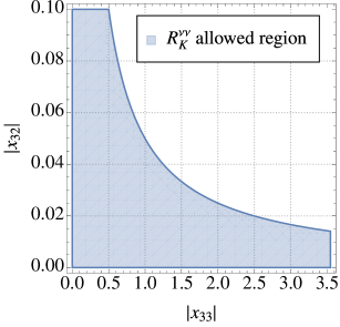
where we have assumed Arg(xi2xi3)=Arg(VtbVts)Argsuperscriptsubscript𝑥𝑖2subscript𝑥𝑖3Argsubscript𝑉𝑡𝑏superscriptsubscript𝑉𝑡𝑠\text{Arg}(x_{i2}^{*}x_{i3})=\text{Arg}(V_{tb}V_{ts}^{*}). We emphasize that this bound represents an insufficient condition for the model to respect the experimental limits. In Fig. 8 we present the allowed region for non-zero x32subscript𝑥32x_{32} and x33subscript𝑥33x_{33} and mϕ=1 TeVsubscript𝑚italic-ϕ1 TeVm_{\phi}=1\text{ TeV}—a coupling texture interesting for explaining RD()subscript𝑅superscript𝐷R_{D^{(*)}}, although heavily constrained by RKννsuperscriptsubscript𝑅𝐾𝜈𝜈R_{K}^{\nu\nu}.

Refer to caption
Figure 8: The region allowed by experimental limits on the decay BKνν𝐵𝐾𝜈𝜈B\to K\nu\nu in the |x33|subscript𝑥33|x_{33}||x32|subscript𝑥32|x_{32}| plane for mϕ=1 TeVsubscript𝑚italic-ϕ1 TeVm_{\phi}=1\text{ TeV}. All other couplings are switched off. A large value of |x33|subscript𝑥33|x_{33}| is essential to explaining RD()subscript𝑅superscript𝐷R_{D^{(*)}}, and the figure implies that such a requirement keeps |x32|subscript𝑥32|x_{32}| small.

The decay K+π+ννsuperscript𝐾superscript𝜋𝜈𝜈K^{+}\rightarrow\pi^{+}\nu\nu constitutes the most stringent constraint on our model from the kaon sector Kumar:2016omp . We find

Br(K+π+νν)=13ijκ+[(ImVtsVtdsw2C2,L21ijλ5)2+(ReVtbVtssw2C2,L21ijλ5+P(u,c)δij)2],Brsuperscript𝐾superscript𝜋𝜈𝜈13subscript𝑖𝑗subscript𝜅delimited-[]superscriptImsubscript𝑉𝑡𝑠superscriptsubscript𝑉𝑡𝑑superscriptsubscript𝑠𝑤2superscriptsubscript𝐶2𝐿21𝑖𝑗superscript𝜆52superscriptResubscript𝑉𝑡𝑏superscriptsubscript𝑉𝑡𝑠superscriptsubscript𝑠𝑤2superscriptsubscript𝐶2𝐿21𝑖𝑗superscript𝜆5subscript𝑃𝑢𝑐subscript𝛿𝑖𝑗2\begin{split}\text{Br}(K^{+}\rightarrow\pi^{+}\nu\nu)&=\frac{1}{3}\sum_{ij}\kappa_{+}\left[\left(\text{Im}\frac{V_{ts}V_{td}^{*}s_{w}^{2}C_{2,L}^{21ij}}{\lambda^{5}}\right)^{2}\right.\\ &\quad\left.+\left(\text{Re}\frac{V_{tb}V_{ts}^{*}s_{w}^{2}C_{2,L}^{21ij}}{\lambda^{5}}+P_{(u,c)}\delta_{ij}\right)^{2}\right],\end{split} (41)

by adapting Eq. (3.29) of Ref. Altmannshofer:2009ma , where the factor κ+=(5.27±0.03)1011subscript𝜅plus-or-minus5.270.03superscript1011\kappa_{+}=(5.27\pm 0.03)\cdot 10^{-11} is due mainly to hadronic matrix elements, λ𝜆\lambda is the CKM Wolfenstein parameter, P(u,c)=0.41±0.05subscript𝑃𝑢𝑐plus-or-minus0.410.05P_{(u,c)}=0.41\pm 0.05 accounts for the effects of light-quark loops, and the small electromagnetic corrections have been neglected. The branching ratio for the decay has most recently been measured by the E949 collaboration to be Br(K+π+νν)=(1.731.05+1.15)1010Brsuperscript𝐾superscript𝜋𝜈𝜈subscriptsuperscript1.731.151.05superscript1010\text{Br}(K^{+}\rightarrow\pi^{+}\nu\nu)=(1.73^{+1.15}_{-1.05})\cdot 10^{-10} Artamonov:2009sz . A conservative limit can be placed on the combination of new-physics couplings featuring in C2,L21ijsuperscriptsubscript𝐶2𝐿21𝑖𝑗C_{2,L}^{21ij} by considering only same-flavored neutrinos in the final state of the decay. Under the assumptions that the couplings involved are real and that only one combination dominates, we find

9.1104<[𝐱𝐱]21m^ϕ2<4.8104.9.1superscript104subscriptdelimited-[]superscript𝐱𝐱21superscriptsubscript^𝑚italic-ϕ24.8superscript104-9.1\cdot 10^{-4}<\frac{[\mathbf{x}^{\dagger}\mathbf{x}]_{21}}{\hat{m}_{\phi}^{2}}<4.8\cdot 10^{-4}. (42)

This bound can be avoided by considering a suppression of the leptoquark couplings to the first generation of quarks.

In this leptoquark model, the coupling of the c𝑐c-quark to the charged leptons is essential for the explanation of the bcτν𝑏𝑐𝜏𝜈b\to c\tau\nu anomalies. Also, as discussed earlier, the up-quark couplings cannot be entirely avoided due to the stringency of Eq. (42) and the mixing of Eq. (8). These factors make the physics of operators of the form 𝒪ijkl(uiΓuj)(kΓl)similar-tosubscript𝒪𝑖𝑗𝑘𝑙subscript𝑢𝑖Γsubscript𝑢𝑗subscript𝑘Γsubscript𝑙\mathscr{O}_{ijkl}\sim(u_{i}\Gamma u_{j})(\ell_{k}\Gamma\ell_{l}) an important source of constraint on this model. Additionally, in order to ensure CLLϕ1.2superscriptsubscript𝐶𝐿𝐿italic-ϕ1.2C_{LL}^{\phi}\approx-1.2 in the model’s original conception, an ansatz for zijsubscript𝑧𝑖𝑗z_{ij} was chosen such that |z22|subscript𝑧22|z_{22}| takes 𝒪(1)𝒪1\mathscr{O}(1) values. Constraints from the decays D0μμsuperscript𝐷0𝜇𝜇D^{0}\rightarrow\mu\mu and D+π+μμsuperscript𝐷superscript𝜋𝜇𝜇D^{+}\rightarrow\pi^{+}\mu\mu are especially worrying in this case, since the leptoquark mediates these processes at tree-level. Even within the context of vanishing first-generation couplings, one cannot avoid inducing new-physics interactions involving up quarks because of the mixing of Eq. (8). The new-physics contributions to decays of the form uiujklsubscript𝑢𝑖subscript𝑢𝑗subscript𝑘subscript𝑙u_{i}\to u_{j}\ell_{k}\ell_{l} can be contained within the effective Lagrangian

3ijkl=4GF2[C3,VRijkl(u¯iγμPRuj)(¯kγμPRl)+C3,VLijkl(u¯iγμPLuj)(¯kγμPLl)+C3,Tijkl(u¯iσμνPRuj)(¯kσμνPRl)+C3,SLijkl(u¯iPLuj)(¯kPLl)+C3,SRijkl(u¯iPRuj)(¯kPRl)+h.c.],superscriptsubscript3𝑖𝑗𝑘𝑙4subscript𝐺𝐹2delimited-[]subscriptsuperscript𝐶𝑖𝑗𝑘𝑙3subscript𝑉𝑅subscript¯𝑢𝑖subscript𝛾𝜇subscript𝑃𝑅subscript𝑢𝑗subscript¯𝑘superscript𝛾𝜇subscript𝑃𝑅subscript𝑙superscriptsubscript𝐶3subscript𝑉𝐿𝑖𝑗𝑘𝑙subscript¯𝑢𝑖subscript𝛾𝜇subscript𝑃𝐿subscript𝑢𝑗subscript¯𝑘superscript𝛾𝜇subscript𝑃𝐿subscript𝑙superscriptsubscript𝐶3𝑇𝑖𝑗𝑘𝑙subscript¯𝑢𝑖subscript𝜎𝜇𝜈subscript𝑃𝑅subscript𝑢𝑗subscript¯𝑘superscript𝜎𝜇𝜈subscript𝑃𝑅subscript𝑙superscriptsubscript𝐶3subscript𝑆𝐿𝑖𝑗𝑘𝑙subscript¯𝑢𝑖subscript𝑃𝐿subscript𝑢𝑗subscript¯𝑘subscript𝑃𝐿subscript𝑙superscriptsubscript𝐶3subscript𝑆𝑅𝑖𝑗𝑘𝑙subscript¯𝑢𝑖subscript𝑃𝑅subscript𝑢𝑗subscript¯𝑘subscript𝑃𝑅subscript𝑙h.c.\begin{split}\mathscr{L}_{3}^{ijkl}&=\frac{4G_{F}}{\sqrt{2}}\bigg{[}C^{ijkl}_{3,V_{R}}(\bar{u}_{i}\gamma_{\mu}P_{R}u_{j})(\bar{\ell}_{k}\gamma^{\mu}P_{R}\ell_{l})+C_{3,V_{L}}^{ijkl}(\bar{u}_{i}\gamma_{\mu}P_{L}u_{j})(\bar{\ell}_{k}\gamma^{\mu}P_{L}\ell_{l})\\ &\quad+C_{3,T}^{ijkl}(\bar{u}_{i}\sigma_{\mu\nu}P_{R}u_{j})(\bar{\ell}_{k}\sigma^{\mu\nu}P_{R}\ell_{l})+C_{3,S_{L}}^{ijkl}(\bar{u}_{i}P_{L}u_{j})(\bar{\ell}_{k}P_{L}\ell_{l})\\ &\quad+C_{3,S_{R}}^{ijkl}(\bar{u}_{i}P_{R}u_{j})(\bar{\ell}_{k}P_{R}\ell_{l})+\text{h.c.}\bigg{]},\end{split} (43)

with coefficients C3,isubscript𝐶3𝑖C_{3,i} at the leptoquark mass scale given by

C3,{VL,VR}ijklsuperscriptsubscript𝐶3subscript𝑉𝐿subscript𝑉𝑅𝑖𝑗𝑘𝑙\displaystyle C_{3,\{V_{L},V_{R}\}}^{ijkl} =122GF{zkjzliykjyli}12mϕ2,absent122subscript𝐺𝐹matrixsubscript𝑧𝑘𝑗superscriptsubscript𝑧𝑙𝑖subscriptsuperscript𝑦𝑘𝑗subscript𝑦𝑙𝑖12superscriptsubscript𝑚italic-ϕ2\displaystyle=\frac{1}{2\sqrt{2}G_{F}}\left\{\begin{matrix}z_{kj}z_{li}^{*}\\ y^{*}_{kj}y_{li}\end{matrix}\right\}\frac{1}{2m_{\phi}^{2}}, (44)
C3,{SL,SR}ijklsuperscriptsubscript𝐶3subscript𝑆𝐿subscript𝑆𝑅𝑖𝑗𝑘𝑙\displaystyle C_{3,\{S_{L},S_{R}\}}^{ijkl} =122GF{zkjyliykjzli}12mϕ2,absent122subscript𝐺𝐹matrixsubscript𝑧𝑘𝑗subscript𝑦𝑙𝑖subscriptsuperscript𝑦𝑘𝑗subscriptsuperscript𝑧𝑙𝑖12superscriptsubscript𝑚italic-ϕ2\displaystyle=\frac{1}{2\sqrt{2}G_{F}}\left\{\begin{matrix}z_{kj}y_{li}\\ y^{*}_{kj}z^{*}_{li}\end{matrix}\right\}\frac{1}{2m_{\phi}^{2}}, (45)
C3,Tijklsuperscriptsubscript𝐶3𝑇𝑖𝑗𝑘𝑙\displaystyle C_{3,T}^{ijkl} =14C3,SLijkl.absent14subscriptsuperscript𝐶𝑖𝑗𝑘𝑙3subscript𝑆𝐿\displaystyle=-\frac{1}{4}C^{ijkl}_{3,S_{L}}. (46)

For the scalar and tensor operators we account for the running of αssubscript𝛼𝑠\alpha_{s} down to the charm-quark mass scale as in Sec. 3.2.1.

For the leptonic decay, we find

Γ(D0μμ)=fD2mD3GF232π(mDmc)2βμ[|C3,SL2122C3,SR2122|2βμ2+|C3,SL2122+C3,SR21222mμmcmD2(C3,VL2122+C3,VR2122)|2]Γsuperscript𝐷0𝜇𝜇superscriptsubscript𝑓𝐷2superscriptsubscript𝑚𝐷3superscriptsubscript𝐺𝐹232𝜋superscriptsubscript𝑚𝐷subscript𝑚𝑐2subscript𝛽𝜇delimited-[]superscriptsuperscriptsubscript𝐶3subscript𝑆𝐿2122superscriptsubscript𝐶3subscript𝑆𝑅21222superscriptsubscript𝛽𝜇2superscriptsuperscriptsubscript𝐶3subscript𝑆𝐿2122superscriptsubscript𝐶3subscript𝑆𝑅21222subscript𝑚𝜇subscript𝑚𝑐superscriptsubscript𝑚𝐷2superscriptsubscript𝐶3subscript𝑉𝐿2122superscriptsubscript𝐶3subscript𝑉𝑅21222\displaystyle\begin{split}\Gamma(D^{0}\rightarrow\mu\mu)&=\frac{f_{D}^{2}m_{D}^{3}G_{F}^{2}}{32\pi}\left(\frac{m_{D}}{m_{c}}\right)^{2}\beta_{\mu}\Bigg{[}\left|C_{3,S_{L}}^{2122}-C_{3,S_{R}}^{2122}\right|^{2}\beta_{\mu}^{2}\\ &\quad+\left|C_{3,S_{L}}^{2122}+C_{3,S_{R}}^{2122}-\frac{2m_{\mu}m_{c}}{m_{D}^{2}}(C_{3,V_{L}}^{2122}+C_{3,V_{R}}^{2122})\right|^{2}\Bigg{]}\end{split} (47a)
=fD2mD3512πmϕ4(mDmc)2βμ[|y22z21z22y21|2βμ2η2+|η(y22z21+z22y21)2mμmcmD2(z22z21+y22y21)|2],absentsuperscriptsubscript𝑓𝐷2superscriptsubscript𝑚𝐷3512𝜋superscriptsubscript𝑚italic-ϕ4superscriptsubscript𝑚𝐷subscript𝑚𝑐2subscript𝛽𝜇delimited-[]superscriptsubscriptsuperscript𝑦22superscriptsubscript𝑧21subscript𝑧22subscript𝑦212superscriptsubscript𝛽𝜇2superscript𝜂2superscript𝜂superscriptsubscript𝑦22superscriptsubscript𝑧21subscript𝑧22subscript𝑦212subscript𝑚𝜇subscript𝑚𝑐superscriptsubscript𝑚𝐷2subscript𝑧22superscriptsubscript𝑧21superscriptsubscript𝑦22subscript𝑦212\displaystyle\begin{split}&=\frac{f_{D}^{2}m_{D}^{3}}{512\pi m_{\phi}^{4}}\left(\frac{m_{D}}{m_{c}}\right)^{2}\beta_{\mu}\left[\vphantom{\frac{2m_{\mu}m_{c}}{m_{D}^{2}}}|y^{*}_{22}z_{21}^{*}-z_{22}y_{21}|^{2}\beta_{\mu}^{2}\eta^{2}\right.\\ &\quad\left.+\left|\eta(y_{22}^{*}z_{21}^{*}+z_{22}y_{21})-\frac{2m_{\mu}m_{c}}{m_{D}^{2}}(z_{22}z_{21}^{*}+y_{22}^{*}y_{21})\right|^{2}\right]\;,\end{split} (47b)

where βμ=(14mμ2/mD2)1/20.99subscript𝛽𝜇superscript14superscriptsubscript𝑚𝜇2superscriptsubscript𝑚𝐷2120.99\beta_{\mu}=(1-4m_{\mu}^{2}/m_{D}^{2})^{1/2}\approx 0.99, fD=212(2) MeVsubscript𝑓𝐷2122 MeVf_{D}=212(2)\text{ MeV} Aoki:2016frl and η=C3,SL2122(mc¯)/C3,SL2122(mϕ)𝜂superscriptsubscript𝐶3subscript𝑆𝐿2122¯subscript𝑚𝑐superscriptsubscript𝐶3subscript𝑆𝐿2122subscript𝑚italic-ϕ\eta=C_{3,S_{L}}^{2122}(\overline{m_{c}})/C_{3,S_{L}}^{2122}(m_{\phi}). In the limit that the left-handed contribution dominates, the bound

|x22|<0.46m^ϕsubscript𝑥220.46subscript^𝑚italic-ϕ|x_{22}|<0.46\hat{m}_{\phi} (48)

can be derived from the experimental upper limit Br(D0μμ)<7.6109Brsuperscript𝐷0𝜇𝜇7.6superscript109\text{Br}(D^{0}\rightarrow\mu\mu)<7.6\cdot 10^{-9} Aaij:2013cza assuming x23x22much-less-thansubscript𝑥23subscript𝑥22x_{23}\ll x_{22}. One can arrange for a mild cancellation between the same- and mixed-chirality terms in Eq. (47) by allowing the right-handed couplings y2(1,2)subscript𝑦212y_{2(1,2)} to take 𝒪(0.1)𝒪0.1\mathscr{O}(0.1) values, however this creates tensions with other meson decays such as Dsμνsubscript𝐷𝑠𝜇𝜈D_{s}\rightarrow\mu\nu, Kμν𝐾𝜇𝜈K\rightarrow\mu\nu and D+π+μμsuperscript𝐷superscript𝜋𝜇𝜇D^{+}\rightarrow\pi^{+}\mu\mu, and we find no overlapping allowed region.

For the decay D+π+μμsuperscript𝐷superscript𝜋𝜇𝜇D^{+}\to\pi^{+}\mu\mu, we implement the calculation of Ref. Fajfer:2015mia . The branching ratio

Br(D+π+μ+μ)<8.3108,Brsuperscript𝐷superscript𝜋superscript𝜇superscript𝜇8.3superscript108\text{Br}(D^{+}\to\pi^{+}\mu^{+}\mu^{-})<8.3\cdot 10^{-8}, (49)

is measured by extrapolating spectra over the resonant region Aaij:2013sua , while the bounds on the separate high- and low-q2superscript𝑞2q^{2} bins are

Br(D+π+μ+μ)q2[1.56,4.00]Brsubscriptsuperscript𝐷superscript𝜋superscript𝜇superscript𝜇superscript𝑞21.564.00\displaystyle\text{Br}(D^{+}\to\pi^{+}\mu^{+}\mu^{-})_{q^{2}\in[1.56,4.00]} <2.9108,absent2.9superscript108\displaystyle<2.9\cdot 10^{-8}, (50)
Br(D+π+μ+μ)q2[0.0625,0.276]Brsubscriptsuperscript𝐷superscript𝜋superscript𝜇superscript𝜇superscript𝑞20.06250.276\displaystyle\text{Br}(D^{+}\to\pi^{+}\mu^{+}\mu^{-})_{q^{2}\in[0.0625,0.276]} <2.5108,absent2.5superscript108\displaystyle<2.5\cdot 10^{-8}, (51)

where q2superscript𝑞2q^{2} ranges are given in GeV2. Both Eq. (50) and Eq. (51) are imposed in our numerical scans.

3.2.4 Meson mixing

A complementary constraint on the left-handed couplings can be derived from Bssubscript𝐵𝑠B_{s}B¯ssubscript¯𝐵𝑠\bar{B}_{s} mixing, providing a stronger bound than RKννsuperscriptsubscript𝑅𝐾𝜈𝜈R_{K}^{\nu\nu} for leptoquark masses larger than a few TeV. The UTfit collaboration determines constraints on ΔF=2Δ𝐹2\Delta F=2 processes in terms of the quotient of the meson mixing amplitude and the SM prediction:

CBse2iϕBsBs|ΔF=2|B¯sBs|SMΔF=2|B¯s,subscript𝐶subscript𝐵𝑠superscript𝑒2𝑖subscriptitalic-ϕsubscript𝐵𝑠quantum-operator-productsubscript𝐵𝑠superscriptΔ𝐹2subscript¯𝐵𝑠quantum-operator-productsubscript𝐵𝑠subscriptsuperscriptΔ𝐹2SMsubscript¯𝐵𝑠C_{B_{s}}e^{2i\phi_{B_{s}}}\equiv\frac{\langle B_{s}|\mathscr{H}^{\Delta F=2}|\bar{B}_{s}\rangle}{\langle B_{s}|\mathscr{H}^{\Delta F=2}_{\text{SM}}|\bar{B}_{s}\rangle}, (52)

and the current best fit values for these parameters are CBs=1.052±0.084subscript𝐶subscript𝐵𝑠plus-or-minus1.0520.084C_{B_{s}}=1.052\pm 0.084 and ϕBs=(0.72±2.06)subscriptitalic-ϕsubscript𝐵𝑠superscriptplus-or-minus0.722.06\phi_{B_{s}}=(0.72\pm 2.06)^{\circ} Bona:2007vi . In the notation of Ref. Bona:2007vi , our leptoquark only generates the effective operator Q1ij=C1bs(q¯iαγμPLqjα)(q¯iβγμPLqjβ)subscriptsuperscript𝑄𝑖𝑗1subscriptsuperscript𝐶𝑏𝑠1subscriptsuperscript¯𝑞𝛼𝑖subscript𝛾𝜇subscript𝑃𝐿superscriptsubscript𝑞𝑗𝛼subscriptsuperscript¯𝑞𝛽𝑖superscript𝛾𝜇subscript𝑃𝐿superscriptsubscript𝑞𝑗𝛽Q^{ij}_{1}=C^{bs}_{1}(\bar{q}^{\alpha}_{i}\gamma_{\mu}P_{L}q_{j}^{\alpha})(\bar{q}^{\beta}_{i}\gamma^{\mu}P_{L}q_{j}^{\beta}), where α𝛼\alpha and β𝛽\beta are color indices, through box diagrams with neutrinos and leptoquarks in the loop. The relevant operator coefficient, defined at the high scale ΛΛ\Lambda, is

C1bs,ϕ(Λ)=1128π2(ixi3xi2mϕ)2,subscriptsuperscript𝐶𝑏𝑠italic-ϕ1Λ1128superscript𝜋2superscriptsubscript𝑖superscriptsubscript𝑥𝑖3subscript𝑥𝑖2subscript𝑚italic-ϕ2C^{bs,\phi}_{1}(\Lambda)=\frac{1}{128\pi^{2}}\left(\sum_{i}\frac{x_{i3}^{*}x_{i2}}{m_{\phi}}\right)^{2}, (53)

in the limit of vanishing SM fermion masses. The SM processes involve similar box diagrams with top quarks and W𝑊W bosons in the loop, inducing the Wilson coefficient (see e.g. Fleischer:2008uj )

C1bs,SM=GF2mW24π2(VtbVts)2S0(mt2/mW2),subscriptsuperscript𝐶𝑏𝑠SM1superscriptsubscript𝐺𝐹2superscriptsubscript𝑚𝑊24superscript𝜋2superscriptsuperscriptsubscript𝑉𝑡𝑏subscript𝑉𝑡𝑠2subscript𝑆0superscriptsubscript𝑚𝑡2superscriptsubscript𝑚𝑊2C^{bs,\text{SM}}_{1}=\frac{G_{F}^{2}m_{W}^{2}}{4\pi^{2}}(V_{tb}^{*}V_{ts})^{2}S_{0}(m_{t}^{2}/m_{W}^{2}), (54)

where S0(x)subscript𝑆0𝑥S_{0}(x) is the well-known Inami-Lim function Inami:1980fz :

S0(x)=x311x2+4x4(x1)23x32(x1)3lnx.subscript𝑆0𝑥superscript𝑥311superscript𝑥24𝑥4superscript𝑥123superscript𝑥32superscript𝑥13𝑥S_{0}(x)=\frac{x^{3}-11x^{2}+4x}{4(x-1)^{2}}-\frac{3x^{3}}{2(x-1)^{3}}\ln x. (55)

We account for the effect of the running of αssubscript𝛼𝑠\alpha_{s} down to mWsubscript𝑚𝑊m_{W} for the coefficient C1bs,ϕsubscriptsuperscript𝐶𝑏𝑠italic-ϕ1C^{bs,\phi}_{1} to compare with the SM result using Aebischer:2017gaw

C1bs,ϕ(mW)=[αs(mt)αs(mW)]γ2β0(5)[αs(Λ)αs(mt)]γ2β0(6)C1bs,ϕ(Λ),superscriptsubscript𝐶1𝑏𝑠italic-ϕsubscript𝑚𝑊superscriptdelimited-[]subscript𝛼𝑠subscript𝑚𝑡subscript𝛼𝑠subscript𝑚𝑊𝛾2superscriptsubscript𝛽05superscriptdelimited-[]subscript𝛼𝑠Λsubscript𝛼𝑠subscript𝑚𝑡𝛾2superscriptsubscript𝛽06superscriptsubscript𝐶1𝑏𝑠italic-ϕΛC_{1}^{bs,\phi}(m_{W})=\left[\frac{\alpha_{s}(m_{t})}{\alpha_{s}(m_{W})}\right]^{\frac{\gamma}{2\beta_{0}^{(5)}}}\left[\frac{\alpha_{s}(\Lambda)}{\alpha_{s}(m_{t})}\right]^{\frac{\gamma}{2\beta_{0}^{(6)}}}C_{1}^{bs,\phi}(\Lambda), (56)

where γ=4𝛾4\gamma=4 and β0(nf)=112nf/3superscriptsubscript𝛽0subscript𝑛𝑓112subscript𝑛𝑓3\beta_{0}^{(n_{f})}=11-2n_{f}/3. The combination of left-handed couplings in Eq. (53) is thus required to satisfy

CBse2iϕBs=1+132GF2mW2S0(mt2/mW2)(ηVtbVtsixi3xi2mϕ)2,subscript𝐶subscript𝐵𝑠superscript𝑒2𝑖subscriptitalic-ϕsubscript𝐵𝑠1132superscriptsubscript𝐺𝐹2superscriptsubscript𝑚𝑊2subscript𝑆0superscriptsubscript𝑚𝑡2superscriptsubscript𝑚𝑊2superscriptsuperscript𝜂superscriptsubscript𝑉𝑡𝑏subscript𝑉𝑡𝑠subscript𝑖superscriptsubscript𝑥𝑖3subscript𝑥𝑖2subscript𝑚italic-ϕ2C_{B_{s}}e^{2i\phi_{B_{s}}}=1+\frac{1}{32G_{F}^{2}m_{W}^{2}S_{0}(m_{t}^{2}/m_{W}^{2})}\left(\frac{\eta^{\prime}}{V_{tb}^{*}V_{ts}}\sum_{i}\frac{x_{i3}^{*}x_{i2}}{m_{\phi}}\right)^{2}, (57)

where η=C1bs,ϕ(mW)/C1bs,ϕ(mϕ)superscript𝜂superscriptsubscript𝐶1𝑏𝑠italic-ϕsubscript𝑚𝑊superscriptsubscript𝐶1𝑏𝑠italic-ϕsubscript𝑚italic-ϕ\eta^{\prime}=C_{1}^{bs,\phi}(m_{W})/C_{1}^{bs,\phi}(m_{\phi}).

3.2.5 Precision electroweak measurements

The Yukawa interactions of the leptoquark with both left- and right-handed SM fermions give corrections to many electroweak observables. Precision measurements of these have been translated into bounds on dimension-six operators in the literature, and we proceed by applying the results of a recent fit to the electroweak precision data Ciuchini:2013pca . Specifically, we consider the way in which the couplings xijsubscript𝑥𝑖𝑗x_{ij} and yijsubscript𝑦𝑖𝑗y_{ij} are constrained by precision electroweak measurements of the Z¯𝑍¯Z\ell\bar{\ell} couplings gLsubscript𝑔𝐿g_{L} and gRsubscript𝑔𝑅g_{R}. These receive corrections from leptoquark loops in our model Bauer:2015knc :

δgIi=(1)δIR332π2mt2mϕ2(lnmϕ2mt21)|λi3I|2132π2mZ2mϕ2j2|λijI|2[(δIL4sw23)(lnmϕ2mZ2+iπ+13)sw29],𝛿superscriptsubscript𝑔𝐼subscript𝑖superscript1subscript𝛿𝐼𝑅332superscript𝜋2superscriptsubscript𝑚𝑡2superscriptsubscript𝑚italic-ϕ2superscriptsubscript𝑚italic-ϕ2superscriptsubscript𝑚𝑡21superscriptsubscriptsuperscript𝜆𝐼𝑖32132superscript𝜋2superscriptsubscript𝑚𝑍2superscriptsubscript𝑚italic-ϕ2superscriptsubscript𝑗2superscriptsubscriptsuperscript𝜆𝐼𝑖𝑗2delimited-[]subscript𝛿𝐼𝐿4superscriptsubscript𝑠𝑤23superscriptsubscript𝑚italic-ϕ2superscriptsubscript𝑚𝑍2𝑖𝜋13superscriptsubscript𝑠𝑤29\begin{split}\delta g_{I}^{\ell_{i}}&=(-1)^{\delta_{IR}}\frac{3}{32\pi^{2}}\frac{m_{t}^{2}}{m_{\phi}^{2}}\left(\ln\frac{m_{\phi}^{2}}{m_{t}^{2}}-1\right)|\lambda^{I}_{i3}|^{2}\\ &\quad-\frac{1}{32\pi^{2}}\frac{m_{Z}^{2}}{m_{\phi}^{2}}\sum_{j}^{2}|\lambda^{I}_{ij}|^{2}\left[\left(\delta_{IL}-\frac{4s_{w}^{2}}{3}\right)\left(\ln\frac{m_{\phi}^{2}}{m_{Z}^{2}}+i\pi+\frac{1}{3}\right)-\frac{s_{w}^{2}}{9}\right],\end{split} (58)

where I{L,R}𝐼𝐿𝑅I\in\{L,R\}, λijL=zijsubscriptsuperscript𝜆𝐿𝑖𝑗subscript𝑧𝑖𝑗\lambda^{L}_{ij}=z_{ij} and λijR=yijsubscriptsuperscript𝜆𝑅𝑖𝑗subscript𝑦𝑖𝑗\lambda^{R}_{ij}=y_{ij}. From Eq. (3.28) and Table 10 of Ref. Ciuchini:2013pca , we calculate the conservative constraints

ReδgLi[8.5,12.0]104,ReδgRi[5.4,6.7]104formulae-sequenceRe𝛿superscriptsubscript𝑔𝐿subscript𝑖8.512.0superscript104Re𝛿superscriptsubscript𝑔𝑅subscript𝑖5.46.7superscript104\text{Re}\delta g_{L}^{\ell_{i}}\in[-8.5,12.0]\cdot 10^{-4},\quad\text{Re}\delta g_{R}^{\ell_{i}}\in[-5.4,6.7]\cdot 10^{-4} (59)

at 95%percent9595\% confidence from the fit results obtained using the large-mtsubscript𝑚𝑡m_{t} expansion. The expressions in Eq. (59) are conservative since we do not account for correlations between different operators but this does not affect our results in an important way. The results of the fit are sensitive to the interference between the SM and leptoquark contributions, hence only the real part of the δgIi𝛿superscriptsubscript𝑔𝐼subscript𝑖\delta g_{I}^{\ell_{i}} is constrained.

4 Results and discussion

Below we study the extent to which the experimental anomalies in RD()subscript𝑅superscript𝐷R_{D^{(*)}}, RK()subscript𝑅superscript𝐾R_{K^{(*)}} and (g2)μsubscript𝑔2𝜇(g-2)_{\mu} can be accommodated in light of the constraints presented in Sec. 3.2. We first consider each anomaly separately and then present the combined parameter space.

For all of the random scans in this section our Monte Carlo strategy proceeds as follows. We sample random real values of the free parameters xijsubscript𝑥𝑖𝑗x_{ij} for i,j1𝑖𝑗1i,j\neq 1 and leptoquark masses in the range m^ϕ[0.6,5]subscript^𝑚italic-ϕ0.65\hat{m}_{\phi}\in[0.6,5]. Values are sampled from the region described in Eq. (40)—a necessary condition for the xijsubscript𝑥𝑖𝑗x_{ij} to respect the bound from BKνν𝐵𝐾𝜈𝜈B\to K\nu\nu, discussed in Sec. 3.2.3—and the perturbativity bound |xij|4πsubscript𝑥𝑖𝑗4𝜋|x_{ij}|\leq\sqrt{4\pi} is imposed at sampling. The values chosen for the right-handed couplings yijsubscript𝑦𝑖𝑗y_{ij} depend on the process studied, although we find that only the y2isubscript𝑦2𝑖y_{2i} and y32subscript𝑦32y_{32} are important for our analysis. Two scans are performed, here labelled I and II. Scan I explores the parameter space associated with RK()subscript𝑅superscript𝐾R_{K^{(*)}} and thus only contains the couplings featuring in Eq. (17), while scan II is intended to elucidate the parameter space associated with both RK()subscript𝑅superscript𝐾R_{K^{(*)}} and RD()subscript𝑅superscript𝐷R_{D^{(*)}}, hence y32subscript𝑦32y_{32} is included. An important difference between scans I and II is that the former allows CLRϕ0superscriptsubscript𝐶𝐿𝑅italic-ϕ0C_{LR}^{\phi}\neq 0, although this comes at the expense of fewer points passing all of the constraints since the couplings y22subscript𝑦22y_{22} and y23subscript𝑦23y_{23} are heavily constrained by semileptonic charged current processes discussed in Sec. 3.2.1. Explicitly, the parameters and respective ranges over which they are scanned are as follows.

Scan I.

61066superscript1066\cdot 10^{6} points sampled from the region in Eq. (40) subject to

  • m^ϕ[0.6,5]subscript^𝑚italic-ϕ0.65\hat{m}_{\phi}\in[0.6,5],

  • |xij|4πsubscript𝑥𝑖𝑗4𝜋|x_{ij}|\leq\sqrt{4\pi} for i,j1𝑖𝑗1{i,j\neq 1},

  • |y22|,|y23|4πsubscript𝑦22subscript𝑦234𝜋|y_{22}|,|y_{23}|\leq\sqrt{4\pi},

  • All other couplings are set to zero.

Of the 61066superscript1066\cdot 10^{6} points, only 5103similar-toabsent5superscript103\sim 5\cdot 10^{3} pass all of the constraints.

Scan II.

61066superscript1066\cdot 10^{6} points sampled from the region in Eq. (40) subject to

  • m^ϕ[0.6,5]subscript^𝑚italic-ϕ0.65\hat{m}_{\phi}\in[0.6,5],

  • |xij|4πsubscript𝑥𝑖𝑗4𝜋|x_{ij}|\leq\sqrt{4\pi} for i,j1𝑖𝑗1{i,j\neq 1},

  • |y23|0.05subscript𝑦230.05|y_{23}|\leq 0.05, |y32|4πsubscript𝑦324𝜋|y_{32}|\leq\sqrt{4\pi},

  • All other couplings, including y22subscript𝑦22y_{22}, are set to zero.

We will see from the results of scan I that y220subscript𝑦220y_{22}\approx 0 is preferred for RK()subscript𝑅superscript𝐾R_{K^{(*)}}, hence we take it to vanish in scan II. The range |y23|0.05subscript𝑦230.05|y_{23}|\leq 0.05 is motivated a posteriori by the fit to (g2)μsubscript𝑔2𝜇(g-2)_{\mu} and the avoidance of a number of constraints. These relaxed requirements on the y2isubscript𝑦2𝑖y_{2i} mean that, of the 61066superscript1066\cdot 10^{6} generated points, 3.7104similar-toabsent3.7superscript104\sim 3.7\cdot 10^{4} pass all of the constraints.

For each of the points the relevant observables and operators RDsubscript𝑅𝐷R_{D}, RDsubscript𝑅superscript𝐷R_{D^{*}}, CLLϕsuperscriptsubscript𝐶𝐿𝐿italic-ϕC_{LL}^{\phi} and CLRϕsuperscriptsubscript𝐶𝐿𝑅italic-ϕC_{LR}^{\phi} are calculated and then the associated coupling constants are filtered through the constraints considered, including RKνν<4.3superscriptsubscript𝑅𝐾𝜈𝜈4.3R_{K}^{\nu\nu}<4.3.

Our analysis mainly focuses on answering the following questions: (1) To what extent can the present leptoquark model explain RK()subscript𝑅superscript𝐾R_{K^{(*)}} while maintaining a SM-like RD()subscript𝑅superscript𝐷R_{D^{(*)}}? (2) To what extent can it explain RD()subscript𝑅superscript𝐷R_{D^{(*)}} with a SM-like RK()subscript𝑅superscript𝐾R_{K^{(*)}}? (3) How well can all of the anomalies be explained together? (4) Can neutrino masses be explained in the regions relevant for the flavor anomalies? Questions (1)–(3) are addressed below in that order, while (4) is addressed in Sec. 4.2. Throughout this discussion, the relative ease with which this leptoquark model can explain the tension in (g2)μsubscript𝑔2𝜇(g-2)_{\mu} is exploited to simplify our study. We do not include its calculation in our numerical scans, since the values of x23subscript𝑥23x_{23} and y23subscript𝑦23y_{23} required—namely, those satisfying Eq. (21)—are such that no constraints are encountered.

4.1 Flavor anomalies

Explaining RK()subscript𝑅superscript𝐾R_{K^{(*)}}.

In order for the leptoquark model to explain the measured tensions in the bs𝑏𝑠b\to s transition the left-handed couplings of ϕitalic-ϕ\phi to the second and third generation of quarks are necessary to ensure a non-vanishing CLLϕsuperscriptsubscript𝐶𝐿𝐿italic-ϕC_{LL}^{\phi}, a parameter space very heavily constrained by the limits from rare meson decays discussed in Sec. 3.2.3. The necessary condition Eq. (40) imposed by the bound on RKννsuperscriptsubscript𝑅𝐾𝜈𝜈R_{K}^{\nu\nu} can be combined with Eq. (17a) to give Bauer:2015knc

i=12|z2i|2+(10.77m^ϕ2)|z23|2(|Vus|2+1)|z22|2+(10.8m^ϕ2)|z23|26CLLϕ.superscriptsubscript𝑖12superscriptsubscript𝑧2𝑖210.77superscriptsubscript^𝑚italic-ϕ2superscriptsubscript𝑧232superscriptsubscript𝑉𝑢𝑠21superscriptsubscript𝑧22210.8superscriptsubscript^𝑚italic-ϕ2superscriptsubscript𝑧232greater-than-or-equivalent-to6superscriptsubscript𝐶𝐿𝐿italic-ϕ\begin{split}\sum_{i=1}^{2}|z_{2i}|^{2}+\left(1-\frac{0.77}{\hat{m}_{\phi}^{2}}\right)|z_{23}|^{2}&\approx\left(|V_{us}|^{2}+1\right)|z_{22}|^{2}+\left(1-\frac{0.8}{\hat{m}_{\phi}^{2}}\right)|z_{23}|^{2}\\ &\gtrsim-6C_{LL}^{\phi}.\end{split} (60)

It follows that 𝒪(1)𝒪1\mathscr{O}(1) couplings to the muon are necessary for the model to meet the benchmark CLLϕ1.2superscriptsubscript𝐶𝐿𝐿italic-ϕ1.2C_{LL}^{\phi}\approx-1.2. For small leptoquark masses the model prefers a large |z22|subscript𝑧22|z_{22}| since the top contribution is suppressed through destructive interference between the box diagrams in Fig. 3, however the limit from D0μμsuperscript𝐷0𝜇𝜇D^{0}\to\mu\mu [see Eq. (48)] prohibits such a scenario. Indeed, the analysis of Ref. Becirevic:2016oho indicates that the constraint following from the LFU evident in RDμ/esuperscriptsubscript𝑅𝐷𝜇𝑒R_{D}^{\mu/e} also constitutes a very serious stumbling-block for the model’s explanation of the bs𝑏𝑠b\to s data for mϕ1 TeVless-than-or-similar-tosubscript𝑚italic-ϕ1 TeVm_{\phi}\lesssim 1\text{ TeV}. We make progress by performing a random scan in which the leptoquark mass is allowed to vary up to 5 TeV5 TeV5\text{ TeV}—such large masses have the effect of lifting the suppression on the last term in Eq. (60) and permitting larger values for z22subscript𝑧22z_{22} according to Eq. (48). In addition to the xijsubscript𝑥𝑖𝑗x_{ij}, we turn on the y2isubscript𝑦2𝑖y_{2i} with i1𝑖1i\neq 1 in order to study the extent to which CLRϕsuperscriptsubscript𝐶𝐿𝑅italic-ϕC_{LR}^{\phi} can contribute. These define the parameters of scan I, introduced above, and we present the results of this scan along with those of scan II, for which CLR=0subscript𝐶𝐿𝑅0C_{LR}=0, in Fig. 9 and Fig. 10. We highlight those points for which the RD()subscript𝑅superscript𝐷R_{D^{(*)}} observables remain SM-like, that is, within twice the theoretical error associated with the SM predictions we cite in Table 1. Consistent with our comments in Section 3.2.1, we find that any phenomenologically viable explanation of the anomalous bs𝑏𝑠b\to s data in this leptoquark model requires mϕ2.5 TeVgreater-than-or-equivalent-tosubscript𝑚italic-ϕ2.5 TeVm_{\phi}\gtrsim 2.5\text{ TeV}. Additionally, constraints from the τμ𝜏𝜇\tau\to\mu flavor-changing observables require |x32|>|x33|subscript𝑥32subscript𝑥33|x_{32}|>|x_{33}| for large |x32|subscript𝑥32|x_{32}|. Although the benchmark value CLLϕ1.2superscriptsubscript𝐶𝐿𝐿italic-ϕ1.2C_{LL}^{\phi}\approx-1.2 is unattainable in light of the constraints we have considered for a perturbative x23subscript𝑥23x_{23}, the model can reduce the tension in RK()subscript𝑅superscript𝐾R_{K^{(*)}} to within 1σ1𝜎1\sigma, a significant improvement on the SM. Points in parameter space implying such large, negative values for CLLϕsuperscriptsubscript𝐶𝐿𝐿italic-ϕC_{LL}^{\phi} also entail a vanishing CLRsubscript𝐶𝐿𝑅C_{LR}, although even in this region agreement with all of the bs𝑏𝑠b\to s data can be slightly better than 3σ3𝜎3\sigma.

Refer to caption
(a) The results of scan I (black) and scan II (red) projected onto the CLLϕsuperscriptsubscript𝐶𝐿𝐿italic-ϕC_{LL}^{\phi}CLRϕsuperscriptsubscript𝐶𝐿𝑅italic-ϕC_{LR}^{\phi} plane. The colored contours correspond to those in Fig. 4: the orange represent the fit to only LFU observables while the blue take into account all bs𝑏𝑠b\to s observables. The model can alleviate the tensions in LFU observables to just within the 1σ1𝜎1\sigma region, a significant improvement on the SM. In this region, CLRϕ0superscriptsubscript𝐶𝐿𝑅italic-ϕ0C_{LR}^{\phi}\approx 0, implying a suppression of the y2isubscript𝑦2𝑖y_{2i}. Agreement with all of the bs𝑏𝑠b\to s data is not as good.
Refer to caption
(b) A scatter plot showing the results of scan II projected onto the CLLϕsuperscriptsubscript𝐶𝐿𝐿italic-ϕC_{LL}^{\phi}m^ϕsubscript^𝑚italic-ϕ\hat{m}_{\phi} plane. Yellow points imply SM-like values for RDsubscript𝑅𝐷R_{D} and RDsubscript𝑅superscript𝐷R_{D^{*}}. The constraints imposed by D0μμsuperscript𝐷0𝜇𝜇D^{0}\to\mu\mu, D+π+μμsuperscript𝐷superscript𝜋𝜇𝜇D^{+}\to\pi^{+}\mu\mu and Zμμ¯𝑍𝜇¯𝜇Z\to\mu\bar{\mu} disfavor light leptoquark masses.
Refer to caption
(c) A scatter plot of CLLϕsuperscriptsubscript𝐶𝐿𝐿italic-ϕC_{LL}^{\phi} against the ratio x33/x23subscript𝑥33subscript𝑥23x_{33}/x_{23} for parameters subject to scan II. Again, yellow points correspond to SM-like RDsubscript𝑅𝐷R_{D} and RDsubscript𝑅superscript𝐷R_{D^{*}}. A large, negative value for CLLϕsuperscriptsubscript𝐶𝐿𝐿italic-ϕC_{LL}^{\phi} requires |x23|>|x33|subscript𝑥23subscript𝑥33|x_{23}|>|x_{33}| to keep LFV τμ𝜏𝜇\tau\to\mu observables at bay.
Figure 9: The key results probing the extent to which the model can explain the tensions in RK()subscript𝑅superscript𝐾R_{K^{(*)}}. Significant improvement from the SM is possible for leptoquark masses between 333 and 5 TeV5 TeV5\text{ TeV}, |x23|>|x33|subscript𝑥23subscript𝑥33|x_{23}|>|x_{33}| and suppressed y2isubscript𝑦2𝑖y_{2i}. The grey areas in (b) and (c) are the 111 and 2σ2𝜎2\sigma allowed regions for RK()subscript𝑅superscript𝐾R_{K^{(*)}}.
Refer to caption
Refer to caption
Refer to caption
Refer to caption
Refer to caption
Refer to caption
Figure 10: Slices through the parameter space investigated through scans I and II. The value of CLLϕsuperscriptsubscript𝐶𝐿𝐿italic-ϕC_{LL}^{\phi} is plotted against each Yukawa coupling scanned over. Plots agains the xijsubscript𝑥𝑖𝑗x_{ij} contain points from scan II and hence 111 and 2σ2𝜎2\sigma regions for RK()subscript𝑅superscript𝐾R_{K^{(*)}} can be specified since CLR=0subscript𝐶𝐿𝑅0C_{LR}=0, these are shaded grey, and points implying SM-like RD()subscript𝑅superscript𝐷R_{D^{(*)}} values are shown in yellow. Plots against the y2isubscript𝑦2𝑖y_{2i} are from scan I, for which all points predict SM-like RD()subscript𝑅superscript𝐷R_{D^{(*)}} since y32=0subscript𝑦320y_{32}=0. Large values of x23subscript𝑥23x_{23} are essential for an adequate explanation of the bs𝑏𝑠b\to s data in this model, while small, but non-zero, values for x22subscript𝑥22x_{22} are necessary to allow CLLϕsuperscriptsubscript𝐶𝐿𝐿italic-ϕC_{LL}^{\phi} to be negative. The values of x23subscript𝑥23x_{23} required to explain the LFU observables to 2σ2𝜎2\sigma begin to impinge on the perturbativity constraint |x23|<4πsubscript𝑥234𝜋|x_{23}|<\sqrt{4\pi}.
Explaining RD()subscript𝑅superscript𝐷R_{D^{(*)}}.

We move on to consider the extent to which the leptoquark can explain the anomalies in the bc𝑏𝑐b\to c transition. The fit presented in Fig. 2 suggests two scenarios for explaining the measured tensions in the bcν𝑏𝑐𝜈b\to c\ell\nu decays in the region A𝐴A: (i) new physics only in CV33superscriptsubscript𝐶𝑉33C_{V}^{33}, or (ii) new-physics in CV33superscriptsubscript𝐶𝑉33C_{V}^{33} along with contributions from CS33superscriptsubscript𝐶𝑆33C_{S}^{33} and CT33superscriptsubscript𝐶𝑇33C_{T}^{33}. Possibility (i) is consistent with the best-fit value, and this is the region of parameter space considered in the model’s original form. However, we emphasize that the conditions presented in Eq. (40) and Eq. (59) are sufficient to preclude that effects in CV33superscriptsubscript𝐶𝑉33C_{V}^{33} alone could be responsible for the enhancement of the RD()subscript𝑅superscript𝐷R_{D^{(*)}} ratios. The product x32x33superscriptsubscript𝑥32subscript𝑥33x_{32}^{*}x_{33} is heavily constrained from RKννsuperscriptsubscript𝑅𝐾𝜈𝜈R_{K}^{\nu\nu} and Bssubscript𝐵𝑠B_{s}B¯ssubscript¯𝐵𝑠\bar{B}_{s} mixing, as indicated in Fig. 8. One could consider generating z23subscript𝑧23z_{23}, and therefore CV33superscriptsubscript𝐶𝑉33C_{V}^{33}, through quark mixing, thus making do only with a non-zero x33subscript𝑥33x_{33} and avoiding these constraints. This set-up, however, requires excessively large values of x33subscript𝑥33x_{33} to explain RD()subscript𝑅superscript𝐷R_{D^{(*)}}, causing the leptoquark’s contributions to the Zττ¯𝑍𝜏¯𝜏Z\tau\bar{\tau} coupling to exceed current experimental limits—a result we illustrate in Fig. 11.
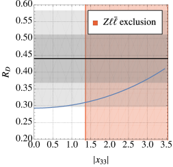
Refer to caption
Refer to caption
Figure 11: The solid blue lines represents the dependence of RDsubscript𝑅𝐷R_{D} (left) and RD()subscript𝑅superscript𝐷R_{D^{(*)}} (right) on |x33|subscript𝑥33|x_{33}| when all other couplings are set to zero and mϕ=1 TeVsubscript𝑚italic-ϕ1 TeVm_{\phi}=1\text{ TeV}. A non-zero x33subscript𝑥33x_{33} generates a small z32subscript𝑧32z_{32} through the quark mixing of Eq. (8), although the |x33|subscript𝑥33|x_{33}| values required to meet the anomalies become large enough to dangerously modify the Zττ𝑍𝜏𝜏Z\to\tau\tau rate. The values of |x33|subscript𝑥33|x_{33}| excluded by measurements of the Zττ𝑍𝜏𝜏Z\tau\tau coupling are shaded red. The solid black line represents the central values of the measurements for RDsubscript𝑅𝐷R_{D} and RD()subscript𝑅superscript𝐷R_{D^{(*)}}, and the grey areas are the 111 and 2σ2𝜎2\sigma regions.

In addition, we find the effects of lepton-flavor violation to be subdued, since such contributions add incoherently to the W𝑊W-mediated SM processes, and thus entail couplings large enough to conflict with measurements of Bssubscript𝐵𝑠B_{s}B¯ssubscript¯𝐵𝑠\bar{B}_{s} mixing and precision electroweak observables. Scenario (ii) involves new physics in CSijsuperscriptsubscript𝐶𝑆𝑖𝑗C_{S}^{ij} and CTijsuperscriptsubscript𝐶𝑇𝑖𝑗C_{T}^{ij}. The most minimal approach here is to turn on only the bottom–tau-neutrino interaction x33subscript𝑥33x_{33} and the right-handed tau–charm coupling y32subscript𝑦32y_{32}. A non-zero x33subscript𝑥33x_{33} will generate CV33superscriptsubscript𝐶𝑉33C_{V}^{33} through quark-mixing. We find the coupling y32subscript𝑦32y_{32} to be weakly constrained by the precision electroweak measurements discussed earlier: in the limit |y32||y3(1,3)|much-greater-thansubscript𝑦32subscript𝑦313|y_{32}|\gg|y_{3(1,3)}|, the bound

|y32|<3.69m^ϕ1+0.39lnm^ϕ,subscript𝑦323.69subscript^𝑚italic-ϕ10.39subscript^𝑚italic-ϕ|y_{32}|<\frac{3.69\hat{m}_{\phi}}{\sqrt{1+0.39\ln\hat{m}_{\phi}}}, (61)

follows from Eq. (59). In addition, small values of the muon–top coupling y23subscript𝑦23y_{23} will allow sizeable contributions to (g2)μsubscript𝑔2𝜇(g-2)_{\mu} in the presence of x230subscript𝑥230x_{23}\neq 0 because of the top-mass enhancement in the mixed-chirality term of Eq. (20). This minimal texture involving only third-generation couplings to left-handed quarks comes with the additional benefit that the leptoquark can evade the constraints from measurements of RKννsuperscriptsubscript𝑅𝐾𝜈𝜈R_{K}^{\nu\nu} and Bssubscript𝐵𝑠B_{s}B¯ssubscript¯𝐵𝑠\bar{B}_{s} mixing. In fact, the only serious constraint is that arising from the modification of the Zττ¯𝑍𝜏¯𝜏Z\tau\bar{\tau} coupling from a large x33subscript𝑥33x_{33}, a situation that can be remedied for y32𝒪(1)similar-tosubscript𝑦32𝒪1y_{32}\sim\mathscr{O}(1), allowing a good fit to the RD()subscript𝑅superscript𝐷R_{D^{(*)}} data for slightly smaller values of x33subscript𝑥33x_{33}. A sizeable y32subscript𝑦32y_{32} is thus a necessary requirement for this leptoquark model to explain the experimental anomalies in RDsubscript𝑅𝐷R_{D} and RDsubscript𝑅superscript𝐷R_{D^{*}}. For example, the parameter choices mϕ=1 TeVsubscript𝑚italic-ϕ1 TeVm_{\phi}=1\text{ TeV}, x33=1.3subscript𝑥331.3x_{33}=1.3 and y32=0.3subscript𝑦320.3y_{32}=0.3 are sufficient to explain RD()subscript𝑅superscript𝐷R_{D^{(*)}} to within 1σ1𝜎1\sigma, and this choice of couplings passes all the constraints we impose. Note also that the measured tension in (g2)μsubscript𝑔2𝜇(g-2)_{\mu} can be accommodated at the same time since the couplings involved are unimportant for bcτν𝑏𝑐𝜏𝜈b\to c\tau\nu. Saturating both x33subscript𝑥33x_{33} and y32subscript𝑦32y_{32} at the perturbativity bound 4π4𝜋\sqrt{4\pi}, we find that an explanation of RD()subscript𝑅superscript𝐷R_{D^{(*)}} loses viability at 10 TeVsimilar-toabsent10 TeV\sim 10\text{ TeV}.

In Fig. 12 we present the results of scan II in the RDsubscript𝑅𝐷R_{D}RDsubscript𝑅superscript𝐷R_{D^{*}} plane, while Fig. 13 displays the values of the Yukawa couplings from the same scan that lead to interesting RDsubscript𝑅𝐷R_{D} values. Limits on the BKνν𝐵𝐾𝜈𝜈B\to K\nu\nu rate and measurements of Bssubscript𝐵𝑠B_{s}B¯ssubscript¯𝐵𝑠\bar{B}_{s} mixing constrain the xi2subscript𝑥𝑖2x_{i2} to be small, while large values for x33subscript𝑥33x_{33} and y32subscript𝑦32y_{32} are necessary since their product appears in the expressions for CV33superscriptsubscript𝐶𝑉33C_{V}^{33}, CS33superscriptsubscript𝐶𝑆33C_{S}^{33} and CT33superscriptsubscript𝐶𝑇33C_{T}^{33}. As discussed above, these large x33subscript𝑥33x_{33} values imply dangerous contributions to Zττ𝑍𝜏𝜏Z\to\tau\tau, causing few points to stray into the 1σ1𝜎1\sigma region. The model can, however, significantly reduce the tension in the bcτν𝑏𝑐𝜏𝜈b\to c\tau\nu measurements in a large region of parameter space. Agreement with the Belle result from Ref. Huschle:2015rga is better than the combined fit, since this model predicts slightly smaller values of RDsubscript𝑅superscript𝐷R_{D^{*}} than those suggested by the BaBar and LHCb measurements.
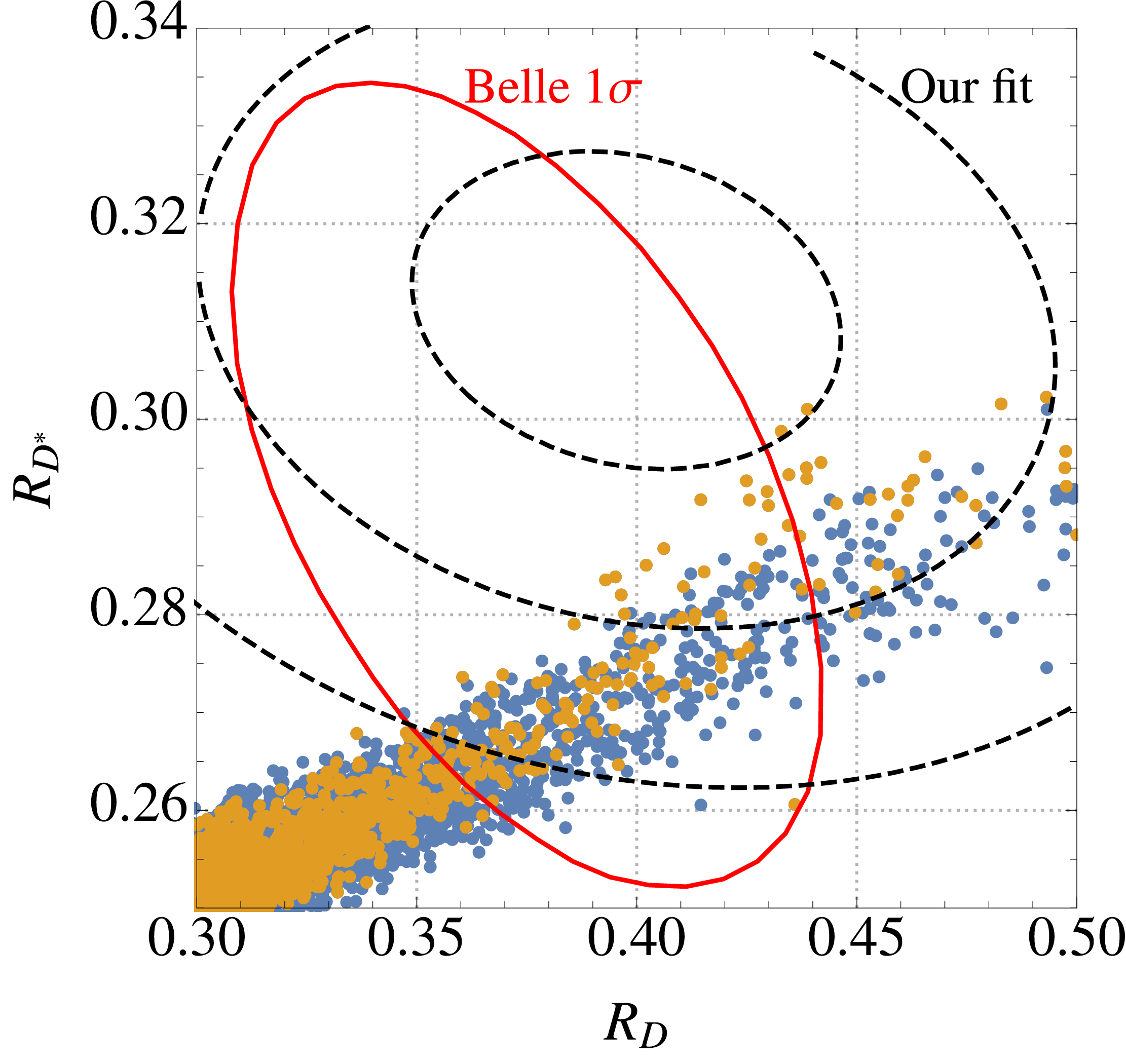
Refer to caption
Figure 12: The results of scan II presented as a scatter plot of RDsubscript𝑅𝐷R_{D} against RDsubscript𝑅superscript𝐷R_{D^{*}}. The orange points keep CLLsubscript𝐶𝐿𝐿C_{LL} SM-like, while blue points show a >1%absentpercent1>1\% deviation in CLLsubscript𝐶𝐿𝐿C_{LL} from the SM prediction. The dashed black ellipses represent the 111, 222 and 3σ3𝜎3\sigma contours from our fit with an assumed correlation ρ=0.2𝜌0.2\rho=-0.2, while the solid red curve indicates the 1σ1𝜎1\sigma allowed region implied by the Belle measurement from Ref. Huschle:2015rga . The anomalies in bcτν𝑏𝑐𝜏𝜈b\to c\tau\nu can be accommodated in this model, although even small, non-zero values for the xi2subscript𝑥𝑖2x_{i2} cause tension with limits from BKνν𝐵𝐾𝜈𝜈B\to K\nu\nu and measurements of Bssubscript𝐵𝑠B_{s}B¯ssubscript¯𝐵𝑠\bar{B}_{s} mixing, causing few points to stray into the 1σ1𝜎1\sigma region of our fit.
Refer to caption
Refer to caption
Refer to caption
Refer to caption
Refer to caption
Refer to caption
Figure 13: Slices through the parameter space of scan II. The solid black line represents the central value of the RDsubscript𝑅𝐷R_{D} measurement, and the grey bands correspond to the 111 and 2σ2𝜎2\sigma regions. The orange points keep CLLsubscript𝐶𝐿𝐿C_{LL} SM-like, while blue points show >1%absentpercent1>1\% deviation in CLLsubscript𝐶𝐿𝐿C_{LL} from the SM prediction. Large values x33subscript𝑥33x_{33} and y32subscript𝑦32y_{32} are necessary for an adequate explanation of RDsubscript𝑅𝐷R_{D} since these feature in CSsubscript𝐶𝑆C_{S} and CTsubscript𝐶𝑇C_{T}. Other left-handed couplings must be small to evade constraints from RKννsuperscriptsubscript𝑅𝐾𝜈𝜈R_{K}^{\nu\nu} and Bssubscript𝐵𝑠B_{s}B¯ssubscript¯𝐵𝑠\bar{B}_{s} mixing. The results for RDsubscript𝑅superscript𝐷R_{D^{*}} are qualitatively the same.
Explaining both RK()subscript𝑅superscript𝐾R_{K^{(*)}} and RD()subscript𝑅superscript𝐷R_{D^{(*)}}.

In order to establish the full power of the model to explain both RD()subscript𝑅superscript𝐷R_{D^{(*)}} and RK()subscript𝑅superscript𝐾R_{K^{(*)}}, we perform a complete scan over the 7-dimensional parameter space spanned by the leptoquark mass and the couplings xijsubscript𝑥𝑖𝑗x_{ij} for i,j1𝑖𝑗1i,j\neq 1, y23subscript𝑦23y_{23} and y32subscript𝑦32y_{32}—the parameters of scan II. Results from this scan have been presented above in the context of explaining one or the other anomaly separately, although in this case the blue points of Figs. 9, 9, 10, 12, 13 and red points of Fig. 9 are relevant. In addition to these, we present the results of scan II in CLLsubscript𝐶𝐿𝐿C_{LL}RDsubscript𝑅𝐷R_{D}RDsubscript𝑅superscript𝐷R_{D^{*}} space, where color is used as the third axis, in Fig. 13. This plot demonstrates a mild tension between RK()subscript𝑅superscript𝐾R_{K^{(*)}} and RD()subscript𝑅superscript𝐷R_{D^{(*)}} in this leptoquark model: points lying within the 1σ1𝜎1\sigma region for RK()subscript𝑅superscript𝐾R_{K^{(*)}} keep RDsubscript𝑅superscript𝐷R_{D^{*}} SM-like, while those breaching the 1σ1𝜎1\sigma boundary for RDsubscript𝑅𝐷R_{D} and RDsubscript𝑅superscript𝐷R_{D^{*}} imply CLLϕ0subscriptsuperscript𝐶italic-ϕ𝐿𝐿0C^{\phi}_{LL}\approx 0. This can be attributed to the behavior evident in Fig. 9: large, negative values of CLLϕsuperscriptsubscript𝐶𝐿𝐿italic-ϕC_{LL}^{\phi} require x330subscript𝑥330x_{33}\approx 0, but x33subscript𝑥33x_{33} is essential to this model’s explanation of RD()subscript𝑅superscript𝐷R_{D^{(*)}}, since it features in CV,S,T33subscriptsuperscript𝐶33𝑉𝑆𝑇C^{33}_{V,S,T}. At best, we find that the model can explain all of the discrepant measurements to within 2σ2𝜎2\sigma, a striking level of consistency with all constraints and anomalies. In both cases the (g2)μsubscript𝑔2𝜇(g-2)_{\mu} anomaly can also be accommodated.

Refer to caption
Figure 14: A projection of the random points subject to scan II onto the RDsubscript𝑅𝐷R_{D}CLLϕsuperscriptsubscript𝐶𝐿𝐿italic-ϕC_{LL}^{\phi} plane, with colors corresponding to σ𝜎\sigma-regions of the fit to RDsubscript𝑅superscript𝐷R_{D^{*}}: black, green, red and blue points lie in the 111, 222, 333 or >3σabsent3𝜎>3\sigma region for RDsubscript𝑅superscript𝐷R_{D^{*}}. The solid black line represents the central value of the RDsubscript𝑅𝐷R_{D} measurement, and the grey bands correspond to the 111 and 2σ2𝜎2\sigma regions. Parameter choices leading to the required large, negative value for CLLϕsuperscriptsubscript𝐶𝐿𝐿italic-ϕC_{LL}^{\phi} tend to compromise agreement with measurements of RDsubscript𝑅superscript𝐷R_{D^{*}}. A combined explanation of RD()subscript𝑅superscript𝐷R_{D^{(*)}} and RK()subscript𝑅superscript𝐾R_{K^{(*)}} is only possible at the 2σ2𝜎2\sigma level for both anomalies. This represents a significant improvement on the SM.

4.2 A representative neutrino mass realization

ν𝜈\nuν𝜈\nuϕasubscriptitalic-ϕ𝑎\phi_{a}b𝑏bb𝑏bϕasubscriptitalic-ϕ𝑎\phi_{a}f𝑓f
Figure 15: Two loop neutrino mass generation in the model of Ref. Angel:2013hla . For simplicity we consider the case where the leptoquark ϕitalic-ϕ\phi couples significantly only to the third generation of quarks. At least two flavors of ϕitalic-ϕ\phi are required to meet the neutrino data.

In this section we incorporate the BN leptoquark into the two-loop neutrino mass model developed and studied in detail in Ref. Angel:2013hla . We summarize the key features of the model below, and point the reader to the original paper for more detail.

Following Ref. Angel:2013hla we couple the leptoquark ϕitalic-ϕ\phi to the color-octet Majorana fermion f(𝟖,𝟏,0)similar-to𝑓810f\sim(\mathbf{8},\mathbf{1},0) in order to introduce the lepton-number violating terms mfffsubscript𝑚𝑓𝑓𝑓m_{f}ff and wid¯ifϕsubscript𝑤𝑖subscript¯𝑑𝑖𝑓italic-ϕw_{i}\bar{d}_{i}f\phi. The dimension-9 ΔL=2Δ𝐿2\Delta L=2 effective operator LLQdcQdc𝐿𝐿𝑄superscript𝑑𝑐𝑄superscript𝑑𝑐LLQd^{c}Qd^{c} is generated when the heavy fields f𝑓f and ϕitalic-ϕ\phi are integrated out. The neutrino mass is proportional to the product of down-type quark mass matrices, which is dominated by the bottom quark mass. We do not consider the case where a strong hierarchy in the wisubscript𝑤𝑖w_{i} undermines this dominance, and thus only the coupling to the third generation of quarks (w3subscript𝑤3w_{3}) is important for the neutrino mass generation. For this reason we set w1,2=0subscript𝑤120w_{1,2}=0 to simplify the calculation of the neutrino mass. In this limit the neutrino mass matrix will have unit rank and an additional generation of the leptoquark ϕitalic-ϕ\phi is needed to satisfy current oscillation data. Replacing ϕitalic-ϕ\phi with ϕa=(ϕ1,ϕ2)subscriptitalic-ϕ𝑎subscriptitalic-ϕ1subscriptitalic-ϕ2\phi_{a}=(\phi_{1},\phi_{2}) in Eq. (5), small neutrino masses are generated through the two-loop graph shown in Fig. 15 and the neutrino mass is given by

Mij4mfmb2(2π)8a,b2(xi3aw3a)Iab(xj3bw3b),subscript𝑀𝑖𝑗4subscript𝑚𝑓superscriptsubscript𝑚𝑏2superscript2𝜋8superscriptsubscript𝑎𝑏2subscript𝑥𝑖3𝑎subscript𝑤3𝑎subscript𝐼𝑎𝑏subscript𝑥𝑗3𝑏subscript𝑤3𝑏M_{ij}\approx 4\frac{m_{f}m_{b}^{2}}{(2\pi)^{8}}\sum_{a,b}^{2}(x_{i3a}w_{3a})I_{ab}(x_{j3b}w_{3b}), (62)

where 𝐈𝐈\mathbf{I} is the matrix of loop integrals in the leptoquark-generation space whose explicit form can be found in Ref. Angel:2013hla . This expression for the mass matrix can be solved for the xi3asubscript𝑥𝑖3𝑎x_{i3a} through the Casas–Ibarra procedure Casas:2001sr to give

xi3a=(2π)42w3ambmfUij[𝐌~1/2]jkRkb[𝐈~1/2𝐒]ba,subscript𝑥𝑖3𝑎superscript2𝜋42subscript𝑤3𝑎subscript𝑚𝑏subscript𝑚𝑓subscriptsuperscript𝑈𝑖𝑗subscriptdelimited-[]superscript~𝐌12𝑗𝑘subscript𝑅𝑘𝑏subscriptdelimited-[]superscript~𝐈12𝐒𝑏𝑎x_{i3a}=\frac{(2\pi)^{4}}{2w_{3a}m_{b}\sqrt{m_{f}}}U^{*}_{ij}[\tilde{\mathbf{M}}^{1/2}]_{jk}R_{kb}[\tilde{\mathbf{I}}^{-1/2}\mathbf{S}]_{ba}, (63)

where tildes denote real and positive diagonal matrices and 𝐒𝐒\mathbf{S} diagonalizes the matrix 𝐈𝐈\mathbf{I}. We use the best-fit values from the NuFIT collaboration for the neutrino mixing angles and mass-squared differences Esteban:2016qun ; nufitweb :

sin2θ12superscript2subscript𝜃12\displaystyle\sin^{2}\theta_{12} =0.306,absent0.306\displaystyle=0.306, Δm212Δsuperscriptsubscript𝑚212\displaystyle\Delta m_{21}^{2} =7.50105 eV2,absent7.50superscript105superscript eV2\displaystyle=7.50\cdot 10^{-5}\text{ eV}^{2}, (64)
sin2θ13superscript2subscript𝜃13\displaystyle\sin^{2}\theta_{13} =0.02166,absent0.02166\displaystyle=0.02166, Δm312Δsuperscriptsubscript𝑚312\displaystyle\Delta m_{31}^{2} =2.524103 eV2 (NO),absent2.524superscript103superscript eV2 (NO)\displaystyle=2.524\cdot 10^{-3}\text{ eV}^{2}\text{ (NO)},
sin2θ23superscript2subscript𝜃23\displaystyle\sin^{2}\theta_{23} =0.441 (NO),absent0.441 (NO)\displaystyle=0.441\text{ (NO)}, Δm322Δsuperscriptsubscript𝑚322\displaystyle\Delta m_{32}^{2} =2.514103 eV2 (IO),absent2.514superscript103superscript eV2 (IO)\displaystyle=-2.514\cdot 10^{-3}\text{ eV}^{2}\text{ (IO)},
sin2θ23superscript2subscript𝜃23\displaystyle\sin^{2}\theta_{23} =0.587 (IO).absent0.587 (IO)\displaystyle=0.587\text{ (IO)}.

The mass-squared differences fix the elements of 𝐌~~𝐌\tilde{\mathbf{M}}, since the lightest neutrino in this model is almost massless. In the cases of normal and inverted neutrino mass hierarchy,

𝐑NO=(00cosθsinθsinθcosθ),𝐑IO=(cosθsinθsinθcosθ00),formulae-sequencesuperscript𝐑NOmatrix00𝜃𝜃𝜃𝜃superscript𝐑IOmatrix𝜃𝜃𝜃𝜃00\mathbf{R}^{\textsc{NO}}=\begin{pmatrix}0&0\\ \cos\theta&-\sin\theta\\ \sin\theta&\cos\theta\end{pmatrix},\quad\mathbf{R}^{\textsc{IO}}=\begin{pmatrix}\cos\theta&-\sin\theta\\ \sin\theta&\cos\theta\\ 0&0\\ \end{pmatrix}, (65)

and θ𝜃\theta\in\mathbb{C} parameterizes the leptoquark–fermion Yukawa couplings through Eq. (63) in such a way that the correct pattern of neutrino masses and mixings is produced. Here we consider the region of parameter space where mϕ2,mfmϕ1much-greater-thansubscript𝑚subscriptitalic-ϕ2subscript𝑚𝑓subscript𝑚subscriptitalic-ϕ1m_{\phi_{2}},m_{f}\gg m_{\phi_{1}} so that ϕ1subscriptitalic-ϕ1\phi_{1} comes to be identified as the BN leptoquark, while ϕ2subscriptitalic-ϕ2\phi_{2} and f𝑓f are effectively divorced from the flavor anomalies. For this reason we refer to ϕ1subscriptitalic-ϕ1\phi_{1} simply as ϕitalic-ϕ\phi and suppress the leptoquark-flavor indices for the remainder of the discussion unless a distinction is necessary. The limit mϕ1mϕ2much-less-thansubscript𝑚subscriptitalic-ϕ1subscript𝑚subscriptitalic-ϕ2m_{\phi_{1}}\ll m_{\phi_{2}} also allows for a simplification in the matrix product 𝐈~1/2𝐒superscript~𝐈12𝐒\tilde{\mathbf{I}}^{-1/2}\mathbf{S} featuring in Eq. (63):

𝐈~1/2𝐒I111/2(ii/ϵ1ϵ),superscript~𝐈12𝐒superscriptsubscript𝐼1112matrix𝑖𝑖italic-ϵ1italic-ϵ\tilde{\mathbf{I}}^{-1/2}\mathbf{S}\approx I_{11}^{-1/2}\begin{pmatrix}-i&i/\epsilon\\ 1&\epsilon\\ \end{pmatrix}, (66)

where ϵI12/I111italic-ϵsubscript𝐼12subscript𝐼11much-less-than1\epsilon\equiv I_{12}/I_{11}\ll 1. This flavor structure implies that its contribution to neutrino mixing is small, and thus the PMNS parameters are principally determined by the Yukawa couplings xi3asubscript𝑥𝑖3𝑎x_{i3a}. We exploit this relative insensitivity to mfsubscript𝑚𝑓m_{f} and mϕ2subscript𝑚subscriptitalic-ϕ2m_{\phi_{2}} to simplify our analysis in the following.

The decoupling of f𝑓f and ϕ2subscriptitalic-ϕ2\phi_{2} from the relevant flavor physics makes w3subscript𝑤3w_{3} an effectively free parameter that acts as a lepton-flavor-blind scaling factor on the couplings of the leptoquark to the third generation of quarks, while θ𝜃\theta governs their relative sizes for a given leptoquark flavor. We plot the xi3subscript𝑥𝑖3x_{i3} against real θ𝜃\theta values in Fig. 16 for the mass choices mf=25 TeVsubscript𝑚𝑓25 TeVm_{f}=25\text{ TeV}, mϕ2=20 TeVsubscript𝑚subscriptitalic-ϕ220 TeVm_{\phi_{2}}=20\text{ TeV} and mϕ1=4 TeVsubscript𝑚subscriptitalic-ϕ14 TeVm_{\phi_{1}}=4\text{ TeV} with fixed w3=0.003subscript𝑤30.003w_{3}=0.003. Both the normal and inverted hierarchies are considered.
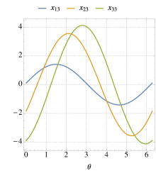
Refer to caption
(a) Normal neutrino mass hierarchy.
Refer to caption
(b) Inverted neutrino mass hierarchy.
Figure 16: Plots of the relative sizes of the couplings of the leptoquark ϕ1subscriptitalic-ϕ1\phi_{1} to the bottom quark and the i𝑖ith neutrino flavor against θ𝜃\theta, the Casas–Ibarra parameter, for mf=25 TeVsubscript𝑚𝑓25 TeVm_{f}=25\text{ TeV}, mϕ2=20 TeVsubscript𝑚subscriptitalic-ϕ220 TeVm_{\phi_{2}}=20\text{ TeV}, mϕ1=4 TeVsubscript𝑚subscriptitalic-ϕ14 TeVm_{\phi_{1}}=4\text{ TeV} and w3=0.003subscript𝑤30.003w_{3}=0.003. We only consider the case θ𝜃\theta\in\mathbb{R} here.

Both Fig. 16 and Eq. (63) indicate that, with the inclusion of neutrino mass, the couplings to the electron and electron-neutrino cannot be turned off ad libitum. Even a small electron coupling z130subscript𝑧130z_{13}\neq 0 can generate dangerous contributions to muon–electron conversion in nuclei in the presence of z230subscript𝑧230z_{23}\neq 0, necessary for the model to alleviate the tensions in the bs𝑏𝑠b\to s transition. We plot the current limit from muon–electron conversion experiments in gold nuclei Br(μ\ceAu79197e\ceAu79197)<7.01013Br𝜇\cesuperscriptsubscriptAu79197𝑒\cesuperscriptsubscriptAu791977.0superscript1013\text{Br}(\mu\ce{{}^{197}_{79}}\text{Au}\to e\ce{{}^{197}_{79}}\text{Au})<7.0\cdot 10^{-13} Olive:2016xmw against θ𝜃\theta and w3subscript𝑤3w_{3} in Fig. 17 for both the normal and inverted hierarchies and a range of masses mϕ1subscript𝑚subscriptitalic-ϕ1m_{\phi_{1}}. The prospective limit from the COMET experiment: Br1016similar-toBrsuperscript1016\text{Br}\sim 10^{-16} Kurup:2011zza , is also shown. A fit to the neutrino oscillation data while respecting measurements of muon–electron conversion implies a fine-tuning in θ𝜃\theta—or, equivalently, z31subscript𝑧31z_{31}—to arrange |z31||z33|much-less-thansubscript𝑧31subscript𝑧33|z_{31}|\ll|z_{33}|, pushing the model into a very specific region of parameter space. The required x310subscript𝑥310x_{31}\approx 0 can be arranged with θ3.08±nπ𝜃plus-or-minus3.08𝑛𝜋\theta\approx 3.08\pm n\pi, fixing the ratio x33/x32=1.96subscript𝑥33subscript𝑥321.96x_{33}/x_{32}=1.96 for the normal neutrino mass hierarchy, and x33/x32=0.85subscript𝑥33subscript𝑥320.85x_{33}/x_{32}=-0.85 for the inverted hierarchy. Comparison with Fig. 9, however, indicates that neither of the aforementioned ratios can allow large contributions to RK()subscript𝑅superscript𝐾R_{K^{(*)}} in the correct direction, although the inverted hierarchy does slightly better than the normal mass ordering. This makes a combined explanation of the bs𝑏𝑠b\to s anomalies and neutrino mass in this model problematic. If, instead, one required that this model explain RD()subscript𝑅superscript𝐷R_{D^{(*)}}, (g2)μsubscript𝑔2𝜇(g-2)_{\mu} and neutrino mass, the values of x33subscript𝑥33x_{33} required are compatible with both the normal and inverted hierarchies, and the model remains agnostic with respect to its preference.
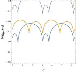
Refer to caption
Figure 17: The figure shows the current (solid) and expected Kurup:2011zza (dashed) limits from muon–electron conversion in nuclei in the θ𝜃\thetaw3subscript𝑤3w_{3} plane for normal mass ordering (blue) and inverted ordering (orange). The region below each curve is ruled out. The dips at θ3.08𝜃3.08\theta\approx 3.08 and θ6.22𝜃6.22\theta\approx 6.22 stretch to negative infinity. Aside from accidental cancellation, the values θ3.08,6.22𝜃3.086.22\theta\approx 3.08,6.22 ensure that the coupling to the electron vanishes. Only real values of θ𝜃\theta are considered.

5 Conclusions

We have reconsidered the potential of a scalar leptoquark ϕ(𝟑,𝟏,1/3)similar-toitalic-ϕ3113\phi\sim(\mathbf{3},\mathbf{1},-1/3) to explain recent B𝐵B-physics anomalies—the LFU ratios RK()subscript𝑅superscript𝐾R_{K^{(*)}} and RD()subscript𝑅superscript𝐷R_{D^{(*)}}, anomalies in branching ratio data and angular observables in the bs𝑏𝑠b\to s transition, as well as the anomalous magnetic moment of the muon.

The leptoquark can reduce the tension in the RD()subscript𝑅superscript𝐷R_{D^{(*)}} observables to within 1σ1𝜎1\sigma of their current experimental values at the price of a sizeable coupling to the right-handed tau and charm quark. The explanation loses viability for masses above about 10 TeV10 TeV10\text{ TeV}. The leptoquark can also reduce the tensions in the bs𝑏𝑠b\to s data, particularly the LFU observables RKsubscript𝑅𝐾R_{K} and RKsubscript𝑅superscript𝐾R_{K^{*}}, albeit at some expense to the explanation of RD()subscript𝑅superscript𝐷R_{D^{(*)}}. Explicitly, the region of parameter space in which RD()subscript𝑅superscript𝐷R_{D^{(*)}} is accommodated to within 1σ1𝜎1\sigma implies RK()subscript𝑅superscript𝐾R_{K^{(*)}} values differing from SM prediction by <1%absentpercent1<1\%, and coupling textures explaining RK()subscript𝑅superscript𝐾R_{K^{(*)}} to within 1σ1𝜎1\sigma keep RD()subscript𝑅superscript𝐷R_{D^{(*)}} within theoretical uncertainty from SM prediction. At best, we find that the model can accommodate the combined tension from both RK()subscript𝑅superscript𝐾R_{K^{(*)}} and RD()subscript𝑅superscript𝐷R_{D^{(*)}} to within 2σ2𝜎2\sigma as well as eliminate the tension in (g2)μsubscript𝑔2𝜇(g-2)_{\mu}, a remarkable feat for a single-particle extension of the SM.

A crucial new ingredient for this model’s explanation of RD()subscript𝑅superscript𝐷R_{D^{(*)}} is the consideration of the area of parameter space in which the coupling y32subscript𝑦32y_{32} is large. The combination of right- and left-handed couplings induces scalar and tensor operators, which lift the chirality suppression of the B𝐵B-meson decays and consequently produce a sizeable new-physics contribution. Moreover the tensor contribution resolves a possible tension induced by the scalar contribution to leptonic charmed B𝐵B-meson decays, Bcτνsubscript𝐵𝑐𝜏𝜈B_{c}\to\tau\nu. In our numerical scans we found that the right-handed Yukawa coupling y32subscript𝑦32y_{32} need take 𝒪(1)𝒪1\mathscr{O}(1) values, while the left-handed couplings x22subscript𝑥22x_{22} and x32subscript𝑥32x_{32} and the right-handed coupling y22subscript𝑦22y_{22} are required to be small. Interestingly, this model predicts a value of RDsubscript𝑅superscript𝐷R_{D^{*}} slightly smaller than that suggested by current data, consistent with the Belle results.

An explanation of RK()subscript𝑅superscript𝐾R_{K^{(*)}} requires 𝒪(1)𝒪1\mathscr{O}(1) couplings of the leptoquark to the muon, a scenario in conflict with the experimental measurements of the decays of the Z𝑍Z boson and D0superscript𝐷0D^{0} mesons in the context of this leptoquark model. Moreover, the tension between RK()subscript𝑅superscript𝐾R_{K^{(*)}} and the lepton universality ratio RD()μ/esuperscriptsubscript𝑅superscript𝐷𝜇𝑒R_{D^{(*)}}^{\mu/e}, pointed out in Ref. Becirevic:2016oho , is naturally relieved for leptoquark masses mϕ1 TeVgreater-than-or-equivalent-tosubscript𝑚italic-ϕ1 TeVm_{\phi}\gtrsim 1\text{ TeV}. Consequently, the best fit to RK()subscript𝑅superscript𝐾R_{K^{(*)}} (requiring large, negative values of CLLϕsuperscriptsubscript𝐶𝐿𝐿italic-ϕC_{LL}^{\phi}) is obtained for large leptoquark masses of 5 TeVsimilar-toabsent5 TeV\sim 5\text{ TeV} with a large hierarchy between the left-handed couplings |x32||x33|much-greater-thansubscript𝑥32subscript𝑥33|x_{32}|\gg|x_{33}| to avoid constraints from τμ𝜏𝜇\tau\to\mu LFV transitions.

Apart from the anomalies in lepton flavor universality ratios, the leptoquark can easily account for the anomalous magnetic moment of the muon by an appropriate choice of the product of couplings y23z23subscript𝑦23subscript𝑧23y_{23}z_{23}. Moreover, the leptoquark appears naturally in models of neutrino mass Mahanta:1999xd ; AristizabalSierra:2007nf ; Angel:2013hla ; Cai:2014kra . We explicitly demonstrate the possibility to explain RD()subscript𝑅superscript𝐷R_{D^{(*)}} in the two-loop neutrino mass model proposed in Ref. Angel:2013hla .

At a future 100 TeV100 TeV100\text{ TeV} proton–proton collider the pair-production cross section of the leptoquark will be substantially enhanced compared to the LHC with about 1 fb1 fb1\text{ fb} for a 5 TeV5 TeV5\text{ TeV} leptoquark Arkani-Hamed:2015vfh and thus will be able to probe most of the relevant parameter space for the B𝐵B-physics anomalies studied here.

Acknowledgments

This work was supported in part by the Australian Research Council. We thank Innes Bigaran, Alexander Ermakov and Phillip Urquijo for discussions on the flavor anomalies. We also thank Damir Bečirević, Christoph Bobeth, Jorge Camalich, Andreas Crivellin, Diptimoy Ghosh, Gudrun Hiller, Soumitra Nandi, Mariano Quiros, Olcyr Sumensari and Javier Virto for helpful correspondence. JG thanks the organisers of the ‘Instant workshop on B𝐵B-meson anomalies’ held at CERN for their hospitality and the many valuable discussions that took place there. All Feynman diagrams were generated using the TikZ-Feynman package for  Ellis:2016jkw .

References

  • (1) G. Hiller and F. Krüger, More model-independent analysis of bs𝑏𝑠b\to s processes, Phys. Rev. D69 (2004) 074020, [hep-ph/0310219].
  • (2) B. Capdevila, A. Crivellin, S. Descotes-Genon, J. Matias and J. Virto, Patterns of New Physics in bs+𝑏𝑠superscriptsuperscriptb\to s\ell^{+}\ell^{-} transitions in the light of recent data, 1704.05340.
  • (3) B. Capdevila, S. Descotes-Genon, J. Matias and J. Virto, Assessing lepton-flavour non-universality from BK𝐵superscript𝐾B\to K^{*}\ell\ell angular analyses, JHEP 10 (2016) 075, [1605.03156].
  • (4) LHCb collaboration, R. Aaij et al., Test of lepton universality using B+K++superscript𝐵superscript𝐾superscriptsuperscriptB^{+}\rightarrow K^{+}\ell^{+}\ell^{-} decays, Phys. Rev. Lett. 113 (2014) 151601, [1406.6482].
  • (5) C. Bobeth, G. Hiller and G. Piranishvili, Angular distributions of B¯K¯+¯𝐵¯𝐾superscriptsuperscript\bar{B}\to\bar{K}\ell^{+}\ell^{-} decays, JHEP 12 (2007) 040, [0709.4174].
  • (6) LHCb collaboration, S. Bifani, Search for new physics with bsl+l𝑏𝑠superscript𝑙superscript𝑙b\to sl^{+}l^{-} decays at lhcb, CERN Seminar 18 April, 2017.
  • (7) M. Bordone, G. Isidori and A. Pattori, On the Standard Model predictions for RKsubscript𝑅𝐾R_{K} and RKsubscript𝑅superscript𝐾R_{K^{*}}, Eur. Phys. J. C76 (2016) 440, [1605.07633].
  • (8) S. Descotes-Genon, J. Matias and J. Virto, Understanding the BKμ+μ𝐵superscript𝐾superscript𝜇superscript𝜇B\to K^{*}\mu^{+}\mu^{-} Anomaly, Phys. Rev. D88 (2013) 074002, [1307.5683].
  • (9) S. Descotes-Genon, L. Hofer, J. Matias and J. Virto, Global analysis of bs𝑏𝑠b\to s\ell\ell anomalies, JHEP 06 (2016) 092, [1510.04239].
  • (10) R. Alonso, B. Grinstein and J. Martin Camalich, SU(2)×U(1)SU2U1\mathrm{SU}(2)\times{}\mathrm{U}(1), Phys. Rev. Lett. 113 (Dec, 2014) 241802.
  • (11) G. Hiller and M. Schmaltz, RKsubscript𝑅𝐾R_{K} and future bs𝑏𝑠b\to s\ell\ell physics beyond the standard model opportunities, Phys. Rev. D90 (2014) 054014, [1408.1627].
  • (12) D. Ghosh, M. Nardecchia and S. A. Renner, Hint of Lepton Flavour Non-Universality in B𝐵B Meson Decays, JHEP 12 (2014) 131, [1408.4097].
  • (13) T. Hurth, F. Mahmoudi and S. Neshatpour, Global fits to bs𝑏𝑠b\to s\ell\ell data and signs for lepton non-universality, JHEP 12 (2014) 053, [1410.4545].
  • (14) W. Altmannshofer and D. M. Straub, New physics in bs𝑏𝑠b\rightarrow s transitions after LHC run 1, Eur. Phys. J. C75 (2015) 382, [1411.3161].
  • (15) S. L. Glashow, D. Guadagnoli and K. Lane, Lepton Flavor Violation in B𝐵B Decays?, Phys. Rev. Lett. 114 (2015) 091801, [1411.0565].
  • (16) W. Altmannshofer, P. Stangl and D. M. Straub, Interpreting Hints for Lepton Flavor Universality Violation, 1704.05435.
  • (17) M. Ciuchini, A. M. Coutinho, M. Fedele, E. Franco, A. Paul, L. Silvestrini et al., On Flavourful Easter eggs for New Physics hunger and Lepton Flavour Universality violation, 1704.05447.
  • (18) L.-S. Geng, B. Grinstein, S. Jäger, J. Martin Camalich, X.-L. Ren and R.-X. Shi, Towards the discovery of new physics with lepton-universality ratios of bs𝑏𝑠b\to s\ell\ell decays, 1704.05446.
  • (19) G. D’Amico, M. Nardecchia, P. Panci, F. Sannino, A. Strumia, R. Torre et al., Flavour anomalies after the RKsubscript𝑅superscript𝐾R_{K^{*}} measurement, 1704.05438.
  • (20) A. Bharucha, D. M. Straub and R. Zwicky, BV+𝐵𝑉superscriptsuperscriptB\to V\ell^{+}\ell^{-} in the Standard Model from light-cone sum rules, JHEP 08 (2016) 098, [1503.05534].
  • (21) J. Lyon and R. Zwicky, Resonances gone topsy turvy - the charm of QCD or new physics in bs+𝑏𝑠superscriptsuperscriptb\to s\ell^{+}\ell^{-}?, 1406.0566.
  • (22) S. Descotes-Genon, L. Hofer, J. Matias and J. Virto, On the impact of power corrections in the prediction of BKμ+μ𝐵superscript𝐾superscript𝜇superscript𝜇B\to K^{*}\mu^{+}\mu^{-} observables, JHEP 12 (2014) 125, [1407.8526].
  • (23) S. Jäger and J. Martin Camalich, Reassessing the discovery potential of the BK+𝐵superscript𝐾superscriptsuperscriptB\to K^{*}\ell^{+}\ell^{-} decays in the large-recoil region: SM challenges and BSM opportunities, Phys. Rev. D93 (2016) 014028, [1412.3183].
  • (24) BaBar collaboration, J. P. Lees et al., Evidence for an excess of B¯D()τν¯τ¯𝐵superscript𝐷superscript𝜏subscript¯𝜈𝜏\bar{B}\to D^{(*)}\tau^{-}\bar{\nu}_{\tau} decays, Phys. Rev. Lett. 109 (2012) 101802, [1205.5442].
  • (25) BaBar collaboration, J. P. Lees et al., Measurement of an Excess of B¯D()τν¯τ¯𝐵superscript𝐷superscript𝜏subscript¯𝜈𝜏\bar{B}\to D^{(*)}\tau^{-}\bar{\nu}_{\tau} Decays and Implications for Charged Higgs Bosons, Phys. Rev. D88 (2013) 072012, [1303.0571].
  • (26) Belle collaboration, M. Huschle et al., Measurement of the branching ratio of B¯D()τν¯τ¯𝐵superscript𝐷superscript𝜏subscript¯𝜈𝜏\bar{B}\to D^{(\ast)}\tau^{-}\bar{\nu}_{\tau} relative to B¯D()ν¯¯𝐵superscript𝐷superscriptsubscript¯𝜈\bar{B}\to D^{(\ast)}\ell^{-}\bar{\nu}_{\ell} decays with hadronic tagging at Belle, Phys. Rev. D92 (2015) 072014, [1507.03233].
  • (27) Belle collaboration, Y. Sato et al., Measurement of the branching ratio of B¯0D+τν¯τsuperscript¯𝐵0superscript𝐷absentsuperscript𝜏subscript¯𝜈𝜏\bar{B}^{0}\rightarrow D^{*+}\tau^{-}\bar{\nu}_{\tau} relative to B¯0D+ν¯superscript¯𝐵0superscript𝐷absentsuperscriptsubscript¯𝜈\bar{B}^{0}\rightarrow D^{*+}\ell^{-}\bar{\nu}_{\ell} decays with a semileptonic tagging method, Phys. Rev. D94 (2016) 072007, [1607.07923].
  • (28) Belle collaboration, S. Hirose et al., Measurement of the τ𝜏\tau lepton polarization and R(D)𝑅superscript𝐷R(D^{*}) in the decay B¯Dτν¯τ¯𝐵superscript𝐷superscript𝜏subscript¯𝜈𝜏\bar{B}\to D^{*}\tau^{-}\bar{\nu}_{\tau}, 1612.00529.
  • (29) LHCb collaboration, R. Aaij et al., Measurement of the ratio of branching fractions (B¯0D+τν¯τ)/(B¯0D+μν¯μ)superscript¯𝐵0superscript𝐷absentsuperscript𝜏subscript¯𝜈𝜏superscript¯𝐵0superscript𝐷absentsuperscript𝜇subscript¯𝜈𝜇\mathcal{B}(\bar{B}^{0}\to D^{*+}\tau^{-}\bar{\nu}_{\tau})/\mathcal{B}(\bar{B}^{0}\to D^{*+}\mu^{-}\bar{\nu}_{\mu}), Phys. Rev. Lett. 115 (2015) 111803, [1506.08614].
  • (30) Y. Sakaki, M. Tanaka, A. Tayduganov and R. Watanabe, Testing leptoquark models in B¯D()τν¯¯𝐵superscript𝐷𝜏¯𝜈\bar{B}\to D^{(*)}\tau\bar{\nu}, Phys. Rev. D88 (2013) 094012, [1309.0301].
  • (31) D. Bardhan, P. Byakti and D. Ghosh, A closer look at the RD and RDsuperscript𝐷{}_{D^{*}} anomalies, JHEP 01 (2017) 125, [1610.03038].
  • (32) M. Freytsis, Z. Ligeti and J. T. Ruderman, Flavor models for B¯D()τν¯¯𝐵superscript𝐷𝜏¯𝜈\bar{B}\to D^{(*)}\tau\bar{\nu}, Phys. Rev. D92 (2015) 054018, [1506.08896].
  • (33) D. Choudhury, A. Kundu, S. Nandi and S. K. Patra, Unified resolution of the R(D)𝑅𝐷R(D) and R(D)𝑅superscript𝐷R(D^{*}) anomalies and the lepton flavor violating decay hμτ𝜇𝜏h\to\mu\tau, Phys. Rev. D95 (2017) 035021, [1612.03517].
  • (34) S. Bhattacharya, S. Nandi and S. K. Patra, Looking for possible new physics in BD()τντ𝐵superscript𝐷𝜏subscript𝜈𝜏B\to D^{(\ast)}\tau\nu_{\tau} in light of recent data, Phys. Rev. D95 (2017) 075012, [1611.04605].
  • (35) S. Bhattacharya, S. Nandi and S. K. Patra, Optimal-observable analysis of possible new physics in BD()τντ𝐵superscript𝐷𝜏subscript𝜈𝜏B\to D^{(\ast)}\tau\nu_{\tau}, Phys. Rev. D93 (2016) 034011, [1509.07259].
  • (36) Heavy Flavor Averaging Group collaboration, Y. Amhis et al., Averages of B-Hadron, C-Hadron, and tau-lepton properties as of early 2012, 1207.1158.
  • (37) MILC collaboration, J. A. Bailey et al., BDν𝐵𝐷𝜈B\to D\ell\nu form factors at nonzero recoil and |Vcb| from 2+1-flavor lattice QCD, Phys. Rev. D92 (2015) 034506, [1503.07237].
  • (38) M. Tanaka and R. Watanabe, New physics in the weak interaction of B¯D()τν¯¯𝐵superscript𝐷𝜏¯𝜈\bar{B}\to D^{(*)}\tau\bar{\nu}, Phys. Rev. D87 (2013) 034028, [1212.1878].
  • (39) R. Alonso, B. Grinstein and J. Martin Camalich, Lepton universality violation and lepton flavor conservation in B𝐵B-meson decays, JHEP 10 (2015) 184, [1505.05164].
  • (40) M. Bauer and M. Neubert, Minimal Leptoquark Explanation for the RD()subscript𝑅superscript𝐷R_{D^{(*)}}, RKsubscript𝑅𝐾R_{K}, and (g2)μsubscript𝑔2𝜇(g-2)_{\mu} Anomalies, Phys. Rev. Lett. 116 (2016) 141802, [1511.01900].
  • (41) D. Bečirević, N. Košnik, O. Sumensari and R. Zukanovich Funchal, Palatable Leptoquark Scenarios for Lepton Flavor Violation in Exclusive bs12𝑏𝑠subscript1subscript2b\to s\ell_{1}\ell_{2} modes, JHEP 11 (2016) 035, [1608.07583].
  • (42) D. Bečirević, S. Fajfer, N. Košnik and O. Sumensari, Leptoquark model to explain the B𝐵B-physics anomalies, RKsubscript𝑅𝐾R_{K} and RDsubscript𝑅𝐷R_{D}, Phys. Rev. D94 (2016) 115021, [1608.08501].
  • (43) S. M. Boucenna, A. Celis, J. Fuentes-Martin, A. Vicente and J. Virto, Non-abelian gauge extensions for B-decay anomalies, Phys. Lett. B760 (2016) 214–219, [1604.03088].
  • (44) S. M. Boucenna, A. Celis, J. Fuentes-Martin, A. Vicente and J. Virto, Phenomenology of an SU(2)×SU(2)×U(1)𝑆𝑈2𝑆𝑈2𝑈1SU(2)\times SU(2)\times U(1) model with lepton-flavour non-universality, JHEP 12 (2016) 059, [1608.01349].
  • (45) L. Calibbi, A. Crivellin and T. Ota, Effective Field Theory Approach to bs()𝑏𝑠superscriptb\to s\ell\ell^{(\prime)}, BK()νν¯𝐵𝐾𝜈¯𝜈B\to K(*)\nu\overline{\nu} and BD()τν𝐵𝐷𝜏𝜈B\to D(*)\tau\nu with Third Generation Couplings, Phys. Rev. Lett. 115 (2015) 181801, [1506.02661].
  • (46) A. Crivellin, D. Müller and T. Ota, Simultaneous Explanation of R(D())𝑅superscript𝐷R(D^{(*)}) and bsμ+μ𝑏𝑠superscript𝜇superscript𝜇b\to s\mu^{+}\mu^{-}: The Last Scalar Leptoquarks Standing, 1703.09226.
  • (47) F. F. Deppisch, S. Kulkarni, H. Päs and E. Schumacher, Leptoquark patterns unifying neutrino masses, flavor anomalies, and the diphoton excess, Phys. Rev. D94 (2016) 013003, [1603.07672].
  • (48) N. G. Deshpande and X.-G. He, Consequences of R-parity violating interactions for anomalies in B¯D()τν¯¯𝐵superscript𝐷𝜏¯𝜈\bar{B}\to D^{(*)}\tau\bar{\nu} and bsμ+μ𝑏𝑠superscript𝜇superscript𝜇b\to s\mu^{+}\mu^{-}, Eur. Phys. J. C77 (2017) 134, [1608.04817].
  • (49) S. Fajfer and N. Košnik, Vector leptoquark resolution of RKsubscript𝑅𝐾R_{K} and RD()subscript𝑅superscript𝐷R_{D^{(*)}} puzzles, Phys. Lett. B755 (2016) 270–274, [1511.06024].
  • (50) F. Feruglio, P. Paradisi and A. Pattori, Revisiting Lepton Flavor Universality in B Decays, Phys. Rev. Lett. 118 (2017) 011801, [1606.00524].
  • (51) F. Feruglio, P. Paradisi and A. Pattori, On the Importance of Electroweak Corrections for B Anomalies, 1705.00929.
  • (52) E. Megias, M. Quiros and L. Salas, Lepton-flavor universality violation in RD()subscript𝑅superscript𝐷R_{D^{(*)}} and RKsubscript𝑅𝐾R_{K} from warped space, 1703.06019.
  • (53) O. Popov and G. A. White, One Leptoquark to unify them? Neutrino masses and unification in the light of (g2)μsubscript𝑔2𝜇(g-2)_{\mu}, RD()subscript𝑅superscript𝐷R_{D^{(\star)}} and RKsubscript𝑅𝐾R_{K} anomalies, 1611.04566.
  • (54) D. Bečirević, S. Fajfer and N. Košnik, Lepton flavor nonuniversality in bs+𝑏𝑠superscriptsuperscriptb\to s\ell^{+}\ell^{-} processes, Phys. Rev. D92 (2015) 014016, [1503.09024].
  • (55) D. Bečirević and O. Sumensari, A leptoquark model to accommodate RKexp<RKSMsuperscriptsubscript𝑅𝐾expsuperscriptsubscript𝑅𝐾SMR_{K}^{\mathrm{exp}}<R_{K}^{\mathrm{SM}} and RKexp<RKSMsuperscriptsubscript𝑅superscript𝐾expsuperscriptsubscript𝑅superscript𝐾SMR_{K^{\ast}}^{\mathrm{exp}}<R_{K^{\ast}}^{\mathrm{SM}}, 1704.05835.
  • (56) A. J. Buras and J. Girrbach, Left-handed Zsuperscript𝑍Z^{\prime} and Z𝑍Z FCNC quark couplings facing new bsμ+μ𝑏𝑠superscript𝜇superscript𝜇b\to s\mu^{+}\mu^{-} data, JHEP 12 (2013) 009, [1309.2466].
  • (57) R. Gauld, F. Goertz and U. Haisch, On minimal Zsuperscript𝑍Z^{\prime} explanations of the BKμ+μ𝐵superscript𝐾superscript𝜇superscript𝜇B\to K^{*}\mu^{+}\mu^{-} anomaly, Phys. Rev. D89 (2014) 015005, [1308.1959].
  • (58) B. Gripaios, M. Nardecchia and S. A. Renner, Composite leptoquarks and anomalies in B𝐵B-meson decays, JHEP 05 (2015) 006, [1412.1791].
  • (59) G. Hiller and M. Schmaltz, Diagnosing lepton-nonuniversality in bs𝑏𝑠b\to s\ell\ell, JHEP 02 (2015) 055, [1411.4773].
  • (60) F. Mahmoudi, S. Neshatpour and J. Virto, BKμ+μ𝐵superscript𝐾superscript𝜇superscript𝜇B\to K^{*}\mu^{+}\mu^{-} optimised observables in the MSSM, Eur. Phys. J. C74 (2014) 2927, [1401.2145].
  • (61) E. Megias, G. Panico, O. Pujolas and M. Quiros, A Natural origin for the LHCb anomalies, JHEP 09 (2016) 118, [1608.02362].
  • (62) H. Päs and E. Schumacher, Common origin of RKsubscript𝑅𝐾R_{K} and neutrino masses, Phys. Rev. D92 (2015) 114025, [1510.08757].
  • (63) S. Sahoo and R. Mohanta, Leptoquark effects on bsνν¯𝑏𝑠𝜈¯𝜈b\to s{{\nu}}\bar{{{\nu}}} and BK+𝐵𝐾superscriptsuperscriptB\to{{K}}\ell^{+}{\ell}^{-} decay processes, New J. Phys. 18 (2016) 013032, [1509.06248].
  • (64) S. Sahoo and R. Mohanta, Study of the rare semileptonic decays Bd0K+superscriptsubscript𝐵𝑑0superscript𝐾superscriptsuperscriptB_{d}^{0}\to K^{*}\ell^{+}\ell^{-} in scalar leptoquark model, Phys. Rev. D93 (2016) 034018, [1507.02070].
  • (65) D. Aristizabal Sierra, F. Staub and A. Vicente, Shedding light on the bs𝑏𝑠b\to s anomalies with a dark sector, Phys. Rev. D92 (2015) 015001, [1503.06077].
  • (66) I. de Medeiros Varzielas and G. Hiller, Clues for flavor from rare lepton and quark decays, JHEP 06 (2015) 072, [1503.01084].
  • (67) S. de Boer and G. Hiller, Flavor and new physics opportunities with rare charm decays into leptons, Phys. Rev. D93 (2016) 074001, [1510.00311].
  • (68) K. S. Babu and C. N. Leung, Classification of effective neutrino mass operators, Nucl. Phys. B619 (2001) 667–689, [hep-ph/0106054].
  • (69) A. de Gouvea and J. Jenkins, A Survey of Lepton Number Violation Via Effective Operators, Phys. Rev. D77 (2008) 013008, [0708.1344].
  • (70) P. W. Angel, N. L. Rodd and R. R. Volkas, Origin of neutrino masses at the LHC: ΔL=2Δ𝐿2\Delta L=2 effective operators and their ultraviolet completions, Phys. Rev. D87 (2013) 073007, [1212.6111].
  • (71) K. Cheung, T. Nomura and H. Okada, Testable radiative neutrino mass model without additional symmetries and explanation for the bs+𝑏𝑠superscriptsuperscriptb\to s\ell^{+}\ell^{-} anomaly, Phys. Rev. D94 (2016) 115024, [1610.02322].
  • (72) K. Cheung, T. Nomura and H. Okada, A Three-loop Neutrino Model with Leptoquark Triplet Scalars, Phys. Lett. B768 (2017) 359–364, [1701.01080].
  • (73) K. Cheung, T. Nomura and H. Okada, Three-loop neutrino mass model with a colored triplet scalar, Phys. Rev. D95 (2017) 015026, [1610.04986].
  • (74) K. S. Babu and J. Julio, Two-Loop Neutrino Mass Generation through Leptoquarks, Nucl. Phys. B841 (2010) 130–156, [1006.1092].
  • (75) D. Aristizabal Sierra, M. Hirsch and S. G. Kovalenko, Leptoquarks: Neutrino masses and accelerator phenomenology, Phys. Rev. D77 (2008) 055011, [0710.5699].
  • (76) P. W. Angel, Y. Cai, N. L. Rodd, M. A. Schmidt and R. R. Volkas, Testable two-loop radiative neutrino mass model based on an LLQdcQdc𝐿𝐿𝑄superscript𝑑𝑐𝑄superscript𝑑𝑐LLQd^{c}Qd^{c} effective operator, JHEP 10 (2013) 118, [1308.0463].
  • (77) I. Doršner, S. Fajfer, A. Greljo, J. F. Kamenik and N. Košnik, Physics of leptoquarks in precision experiments and at particle colliders, Phys. Rept. 641 (2016) 1–68, [1603.04993].
  • (78) CMS collaboration, V. Khachatryan et al., Search for pair production of first and second generation leptoquarks in proton-proton collisions at s=8𝑠8\sqrt{s}=8 TeV, Phys. Rev. D93 (2016) 032004, [1509.03744].
  • (79) ATLAS collaboration, G. Aad et al., Searches for scalar leptoquarks in pp collisions at s𝑠\sqrt{s} = 8 TeV with the ATLAS detector, Eur. Phys. J. C76 (2016) 5, [1508.04735].
  • (80) B. Dumont, K. Nishiwaki and R. Watanabe, LHC constraints and prospects for S1subscript𝑆1S_{1} scalar leptoquark explaining the B¯D()τν¯¯𝐵superscript𝐷𝜏¯𝜈\bar{B}\to D^{(*)}\tau\bar{\nu} anomaly, Phys. Rev. D94 (2016) 034001, [1603.05248].
  • (81) BaBar collaboration, B. Aubert et al., Determination of the form-factors for the decay B0D+νlsuperscript𝐵0superscript𝐷absentsuperscriptsubscript𝜈𝑙B^{0}\to D^{*-}\ell^{+}\nu_{l} and of the CKM matrix element |Vcb|subscript𝑉𝑐𝑏|V_{cb}|, Phys. Rev. D77 (2008) 032002, [0705.4008].
  • (82) BaBar collaboration, B. Aubert et al., Measurements of the Semileptonic Decays B¯Dν¯¯𝐵𝐷¯𝜈\bar{B}\to D\ell\bar{\nu} and B¯Dν¯¯𝐵superscript𝐷¯𝜈\bar{B}\to D^{*}\ell\bar{\nu} Using a Global Fit to DXν¯𝐷𝑋¯𝜈D\to X\ell\bar{\nu} Final States, Phys. Rev. D79 (2009) 012002, [0809.0828].
  • (83) Belle collaboration, K. Abe et al., Measurement of BR(B¯0D+ν¯)𝐵𝑅subscript¯𝐵0superscript𝐷superscript¯𝜈BR(\bar{B}_{0}\to D^{+}\ell^{-}\bar{\nu}) and determination of |Vcb|subscript𝑉𝑐𝑏|V_{cb}|, Phys. Lett. B526 (2002) 258–268, [hep-ex/0111082].
  • (84) Belle collaboration, W. Dungel et al., Measurement of the form factors of the decay B0D+νsubscript𝐵0superscript𝐷superscript𝜈B_{0}\to D^{*}-\ell^{+}\nu and determination of the CKM matrix element |Vcb|subscript𝑉𝑐𝑏|V_{cb}|, Phys. Rev. D82 (2010) 112007, [1010.5620].
  • (85) I. Doršner, S. Fajfer, N. Košnik and I. Nišandžić, Minimally flavored colored scalar in B¯D()τν¯¯𝐵superscript𝐷𝜏¯𝜈\bar{B}\to D^{(*)}\tau\bar{\nu} and the mass matrices constraints, JHEP 11 (2013) 084, [1306.6493].
  • (86) K. G. Chetyrkin, J. H. Kuhn and M. Steinhauser, RunDec: A Mathematica package for running and decoupling of the strong coupling and quark masses, Comput. Phys. Commun. 133 (2000) 43–65, [hep-ph/0004189].
  • (87) M. Misiak, The bse+e𝑏𝑠superscript𝑒superscript𝑒b\to se^{+}e^{-} and bsγ𝑏𝑠𝛾b\to s\gamma decays with next-to-leading logarithmic QCD corrections, Nucl. Phys. B393 (1993) 23–45.
  • (88) BaBar collaboration, J. P. Lees et al., Measurement of the BXs+𝐵subscript𝑋𝑠superscriptsuperscriptB\to X_{s}\ell^{+}\ell^{-} branching fraction and search for direct CP violation from a sum of exclusive final states, Phys. Rev. Lett. 112 (2014) 211802, [1312.5364].
  • (89) A. Djouadi, T. Kohler, M. Spira and J. Tutas, (e b), (e t) type leptoquarks at e p collider, Z. Phys. C46 (1990) 679–686.
  • (90) D. Chakraverty, D. Choudhury and A. Datta, A Nonsupersymmetric resolution of the anomalous muon magnetic moment, Phys. Lett. B506 (2001) 103–108, [hep-ph/0102180].
  • (91) K.-m. Cheung, Muon anomalous magnetic moment and leptoquark solutions, Phys. Rev. D64 (2001) 033001, [hep-ph/0102238].
  • (92) M. Davier, A. Hoecker, B. Malaescu and Z. Zhang, Reevaluation of the Hadronic Contributions to the Muon g2𝑔2g-2 and to α(MZ)𝛼subscript𝑀𝑍\alpha(M_{Z}), Eur. Phys. J. C71 (2011) 1515, [1010.4180].
  • (93) S. Aoki et al., Review of lattice results concerning low-energy particle physics, Eur. Phys. J. C77 (2017) 112, [1607.00299].
  • (94) R. Alonso, B. Grinstein and J. Martin Camalich, The lifetime of the Bcsuperscriptsubscript𝐵𝑐B_{c}^{-} meson and the anomalies in BD()τν𝐵superscript𝐷𝜏𝜈B\to D^{(*)}\tau\nu, Phys. Rev. Lett. 118 (2017) 081802, [1611.06676].
  • (95) Belle collaboration, A. Zupanc et al., Measurements of branching fractions of leptonic and hadronic Ds+superscriptsubscript𝐷𝑠D_{s}^{+} meson decays and extraction of the Ds+superscriptsubscript𝐷𝑠D_{s}^{+} meson decay constant, JHEP 09 (2013) 139, [1307.6240].
  • (96) Belle collaboration, R. Glattauer et al., Measurement of the decay BDν𝐵𝐷subscript𝜈B\to D\ell\nu_{\ell} in fully reconstructed events and determination of the Cabibbo-Kobayashi-Maskawa matrix element |Vcb|subscript𝑉𝑐𝑏|V_{cb}|, Phys. Rev. D93 (2016) 032006, [1510.03657].
  • (97) Belle collaboration, A. Abdesselam et al., Precise determination of the CKM matrix element |Vcb|subscript𝑉𝑐𝑏\left|V_{cb}\right| with B¯0D+ν¯superscript¯𝐵0superscript𝐷absentsuperscriptsubscript¯𝜈\bar{B}^{0}\to D^{*\,+}\,\ell^{-}\,\bar{\nu}_{\ell} decays with hadronic tagging at Belle, 1702.01521.
  • (98) Particle Data Group collaboration, C. Patrignani et al., Review of Particle Physics, Chin. Phys. C40 (2016) 100001.
  • (99) V. Cirigliano and I. Rosell, π/Keν¯e𝜋𝐾𝑒subscript¯𝜈𝑒\pi/K\to e\bar{\nu}_{e} branching ratios to O(e2p4superscript𝑒2superscript𝑝4e^{2}p^{4}) in Chiral Perturbation Theory, JHEP 10 (2007) 005, [0707.4464].
  • (100) M. Finkemeier, Radiative corrections to πl2subscript𝜋𝑙2\pi_{l2} and Kl2subscript𝐾𝑙2K_{l2} decays, hep-ph/9501286.
  • (101) W. Buchmuller and D. Wyler, Constraints on SU(5) Type Leptoquarks, Phys. Lett. B177 (1986) 377–382.
  • (102) S. Davidson, D. C. Bailey and B. A. Campbell, Model independent constraints on leptoquarks from rare processes, Z. Phys. C61 (1994) 613–644, [hep-ph/9309310].
  • (103) X.-Q. Li, Y.-D. Yang and X. Zhang, Revisiting the one leptoquark solution to the R(D())𝑅superscript𝐷R(D^{(*)}) anomalies and its phenomenological implications, JHEP 08 (2016) 054, [1605.09308].
  • (104) BaBar collaboration, B. Aubert et al., Searches for Lepton Flavor Violation in the Decays τ+e+γsuperscript𝜏superscript𝑒𝛾\tau^{+}\to e^{+}\gamma and τ+μ+γsuperscript𝜏superscript𝜇𝛾\tau^{+}\to\mu^{+}\gamma, Phys. Rev. Lett. 104 (2010) 021802, [0908.2381].
  • (105) Belle collaboration, Y. Miyazaki et al., Search for Lepton-Flavor-Violating tau Decays into a Lepton and a Vector Meson, Phys. Lett. B699 (2011) 251–257, [1101.0755].
  • (106) SINDRUM II collaboration, W. H. Bertl et al., A Search for muon to electron conversion in muonic gold, Eur. Phys. J. C47 (2006) 337–346.
  • (107) Y. Cai, J. D. Clarke, M. A. Schmidt and R. R. Volkas, Testing Radiative Neutrino Mass Models at the LHC, JHEP 02 (2015) 161, [1410.0689].
  • (108) W. Altmannshofer, A. J. Buras, D. M. Straub and M. Wick, New strategies for New Physics search in BKνν¯𝐵superscript𝐾𝜈¯𝜈B\to K^{*}\nu\bar{\nu}, BKνν¯𝐵𝐾𝜈¯𝜈B\to K\nu\bar{\nu} and BXsνν¯𝐵subscript𝑋𝑠𝜈¯𝜈B\to X_{s}\nu\bar{\nu} decays, JHEP 04 (2009) 022, [0902.0160].
  • (109) A. J. Buras, F. Schwab and S. Uhlig, Waiting for precise measurements of K+π+νν¯superscript𝐾superscript𝜋𝜈¯𝜈K^{+}\to\pi^{+}\nu\bar{\nu} and KLπ0νν¯subscript𝐾𝐿superscript𝜋0𝜈¯𝜈K_{L}\to\pi^{0}\nu\bar{\nu}, Rev. Mod. Phys. 80 (2008) 965–1007, [hep-ph/0405132].
  • (110) G. Buchalla and A. J. Buras, The rare decays Kπνν¯𝐾𝜋𝜈¯𝜈K\to\pi\nu\bar{\nu}, BXνν¯𝐵𝑋𝜈¯𝜈B\to X\nu\bar{\nu} and B+𝐵superscriptsuperscriptB\to\ell^{+}\ell^{-}: An Update, Nucl. Phys. B548 (1999) 309–327, [hep-ph/9901288].
  • (111) M. Misiak and J. Urban, QCD corrections to FCNC decays mediated by Z penguins and W boxes, Phys. Lett. B451 (1999) 161–169, [hep-ph/9901278].
  • (112) A. J. Buras, J. Girrbach-Noe, C. Niehoff and D. M. Straub, BK()νν¯𝐵superscript𝐾𝜈¯𝜈B\to{K}^{\left(\ast\right)}\nu\overline{\nu} decays in the Standard Model and beyond, JHEP 02 (2015) 184, [1409.4557].
  • (113) G. Kumar, Constraints on a scalar leptoquark from the kaon sector, Phys. Rev. D94 (2016) 014022, [1603.00346].
  • (114) BNL-E949 collaboration, A. V. Artamonov et al., Study of the decay K+π+νν¯superscript𝐾superscript𝜋𝜈¯𝜈K^{+}\to\pi^{+}\nu\bar{\nu} in the momentum region 140<Pπ<199140subscript𝑃𝜋199140<P_{\pi}<199 MeV/c, Phys. Rev. D79 (2009) 092004, [0903.0030].
  • (115) LHCb collaboration, R. Aaij et al., Search for the rare decay D0μ+μsuperscript𝐷0superscript𝜇superscript𝜇D^{0}\to\mu^{+}\mu^{-}, Phys. Lett. B725 (2013) 15–24, [1305.5059].
  • (116) S. Fajfer and N. Košnik, Prospects of discovering new physics in rare charm decays, Eur. Phys. J. C75 (2015) 567, [1510.00965].
  • (117) LHCb collaboration, R. Aaij et al., Search for Ds+π+μ+μsubscriptsuperscript𝐷𝑠superscript𝜋superscript𝜇superscript𝜇D^{+}_{s}\to\pi^{+}\mu^{+}\mu^{-} and Ds+πμ+μ+subscriptsuperscript𝐷𝑠superscript𝜋superscript𝜇superscript𝜇D^{+}_{s}\to\pi^{-}\mu^{+}\mu^{+} decays, Phys. Lett. B724 (2013) 203–212, [1304.6365].
  • (118) UTfit collaboration, M. Bona et al., Model-independent constraints on ΔF=2Δ𝐹2\Delta F=2 operators and the scale of new physics, JHEP 03 (2008) 049, [0707.0636].
  • (119) R. Fleischer, Flavour Physics and CP Violation: Expecting the LHC, in High-energy physics. Proceedings, 4th Latin American CERN-CLAF School, Vina del Mar, Chile, February 18-March 3, 2007, pp. 105–157, 2008. 0802.2882.
  • (120) T. Inami and C. S. Lim, Effects of Superheavy Quarks and Leptons in Low-Energy Weak Processes KLμμ¯subscript𝐾𝐿𝜇¯𝜇K_{L}\to\mu\bar{\mu}, K+π+νν¯superscript𝐾superscript𝜋𝜈¯𝜈K^{+}\to\pi^{+}\nu\bar{\nu} and K0K¯0superscript𝐾0superscript¯𝐾0K^{0}\leftrightarrow\bar{K}^{0}, Prog. Theor. Phys. 65 (1981) 297.
  • (121) J. Aebischer, M. Fael, C. Greub and J. Virto, B physics Beyond the Standard Model at One Loop: Complete Renormalization Group Evolution below the Electroweak Scale, 1704.06639.
  • (122) M. Ciuchini, E. Franco, S. Mishima and L. Silvestrini, Electroweak Precision Observables, New Physics and the Nature of a 126 GeV Higgs Boson, JHEP 08 (2013) 106, [1306.4644].
  • (123) J. A. Casas and A. Ibarra, Oscillating neutrinos and μeγ𝜇𝑒𝛾\mu\to e\gamma, Nucl. Phys. B618 (2001) 171–204, [hep-ph/0103065].
  • (124) I. Esteban, M. C. Gonzalez-Garcia, M. Maltoni, I. Martinez-Soler and T. Schwetz, Updated fit to three neutrino mixing: exploring the accelerator-reactor complementarity, JHEP 01 (2017) 087, [1611.01514].
  • (125) “Nufit 3.0 (2016).” www.nu-fit.org.
  • (126) COMET collaboration, A. Kurup, The COherent Muon to Electron Transition (COMET) experiment, Nucl. Phys. Proc. Suppl. 218 (2011) 38–43.
  • (127) U. Mahanta, Neutrino masses and mixing angles from leptoquark interactions, Phys. Rev. D62 (2000) 073009, [hep-ph/9909518].
  • (128) N. Arkani-Hamed, T. Han, M. Mangano and L.-T. Wang, Physics opportunities of a 100 TeV proton-proton collider, Phys. Rept. 652 (2016) 1–49, [1511.06495].
  • (129) J. Ellis, TikZ-Feynman: Feynman diagrams with TikZ, Comput. Phys. Commun. 210 (2017) 103–123, [1601.05437].