Kernel methods for interpretable machine learning of order parameters
Abstract
Machine learning is capable of discriminating phases of matter, and finding associated phase transitions, directly from large data sets of raw state configurations. In the context of condensed matter physics, most progress in the field of supervised learning has come from employing neural networks as classifiers. Although very powerful, such algorithms suffer from a lack of interpretability, which is usually desired in scientific applications in order to associate learned features with physical phenomena. In this paper, we explore support vector machines (SVMs) which are a class of supervised kernel methods that provide interpretable decision functions. We find that SVMs can learn the mathematical form of physical discriminators, such as order parameters and Hamiltonian constraints, for a set of two-dimensional spin models: the ferromagnetic Ising model, a conserved-order-parameter Ising model, and the Ising gauge theory. The ability of SVMs to provide interpretable classification highlights their potential for automating feature detection in both synthetic and experimental data sets for condensed matter and other many-body systems.
I Introduction
Pattern recognition, the task of automatic discovery of features and regularities in data, is a major focus of machine learning, which now powers many different tools in our daily lives Bishop (2006); Murphy (2012). From a physics perspective, the problem of searching for patterns in experimental data has long driven theoretical progress which, by definition, relates the patterns to underlying postulates of our physical theories. Hence, in the modern push to automate the discovery of important and novel physical features in data Li et al. (2015); Carrasquilla and Melko (2017); Wang (2016); Carleo and Troyer (2017); Torlai and Melko (2016a); Broecker et al. (2016); Ch’ng et al. (2016); Tanaka and Tomiya (2016); Ohtsuki and Ohtsuki (2016); Li et al. (2016); Deng et al. (2016); Huang and Wang (2017); Liu et al. (2017); Torlai and Melko (2016b); van Nieuwenburg et al. (2017); Zhang and Kim (2016); Portman and Tamblyn (2016); Liu et al. (2017); Crawford et al. (2016); Aoki and Kobayashi (2016); Deng et al. (2017); Gao and Duan (2017); Chen et al. (2017); Huang and Moore (2017); Wetzel (2017); Torlai et al. (2017); Hu et al. (2017); Schindler et al. (2017), physicists must be mindful of the interpretability of machine learning results if they are truly meant to drive theoretical process.
In condensed matter, physicists face the ultimate big-data challenge. One must search practical measurements, obtained from the exponentially-large state space of a system or model, for patterns which relate to underlying theoretical paradigms. The recent success of neural networks in classifying phases of matter Carrasquilla and Melko (2017); Broecker et al. (2016); Zhang and Kim (2016); Torlai and Melko (2016a); Carleo and Troyer (2017); Ch’ng et al. (2016); Schindler et al. (2017) has been encouraging, in that it demonstrates how relatively standard supervised learning tools can be repurposed for calculations in condensed matter physics. However, contrary to industry applications of machine learning, where performance is the prime metric of success, in physics it is generally desirable to further tie the outcome to some theoretical structure, which can eventually be used e.g. to make predictions. Neural network behavior can indeed be interpreted on the simplest models of statistical mechanics, such as the demonstration in Ref. Carrasquilla and Melko (2017) that the magnetization order parameter of the two-dimensional (2d) Ising model is learned by the weights of the hidden units. However, in general for more complicated models, similar success in relating network structure to non-linear or non-local order parameters is challenging, especially in the case of deep neural networks. This lack of interpretability presents a challenge for the goal of driving theoretical progress with machine learning. It is therefore crucial that the condensed matter community survey the performance of interpretable machine learning algorithms on data obtained from models of interest to condensed matter physics.
In this paper we study interpretable supervised learning algorithms applied to the discrimination of phases of matter in large synthetic data sets produced by numerical simulation. We focus on a particular class of machine learning algorithms called support vector machines (SVMs). In particular, we ask whether SVMs in the supervised learning setting are able to discover the mathematical structure of physical order parameters. We first introduce the SVM algorithm and describe its general properties, with particular focus on the kernel trick. This trick allows us to perform linear regression on non-linear features of the data, without explicitly generating the features. In particular, this is relevant when applied to Monte Carlo data from many-body systems, which typically have high-dimensional physical states. Without the kernel trick, it would be unpractical to generate a set of non-linear features, which could be exponentially large. In section III, we perform phase classification on Monte Carlo configurations produced from the 2d Ising model, a conserved-order-parameter Ising model (COP) Wang (2016), and the 2d Ising gauge theory. We find that SVMs with a quadratic polynomial kernel can discriminate the phases of the 2d Ising model by learning the correct physical order parameter (the squared magnetization per spin). In the case of COP model, we find that SVMs are able to discover the non-trivial order parameter, devised by Wang Wang (2016) through visualization of dimensionally-reduced data, with less human intervention. Finally, we show that the 2d Ising gauge theory, whose ground state is defined by local plaquette constraints but no conventional order parameter, can be discriminated by SVMs with polynomial kernels. In this case, no polynomial with order less than four can identify the ground state, indicating that the SVM is able to learn the original Hamiltonian in order to evaluate whether the local constraints on four Ising degrees of freedom are satisfied for each plaquette.
II Support Vector Machines
Linear support vector machines Murphy (2012) were initially designed to perform binary classification. They belong to the class of supervised learning algorithms that, given an input , predict the class in which it is most likely to belong. In the context of this paper, the input will represent a spin configuration from a statistical mechanical model of interest in condensed matter physics, in which the different components of , called features in the machine learning literature, correspond to the spins at different lattice sites. The output will label the thermodynamic phase it was sampled from. The main idea behind SVMs is to find the hyperplane, defined by , that best separates the two classes. Formally, this is achieved by solving the optimization problem:
| (1) |
Here, is a constant, are “slack” variables (described more below) and is the number of input samples, called the training set. Finding optimal parameters and , which can then be used to make predictions on a test set, is the goal of supervised learning with SVMs. Unlike say a feed-forward neural network Carrasquilla and Melko (2017), this model does not provide probabilistic predictions. However, the optimization problem Eq. (II) is equivalent to with . Because the hinge function approximates the misclassification error Bishop (2006), this can be viewed as an approximation to minimizing the misclassification error with a so-called -norm regularization (which penalizes unnecessary coefficients of ). This analogy also explicitly shows that can be interpreted as a regularization parameter.
When the variables are constrained to be zero in Eq. (II), this corresponds to the hard margin case and the optimization algorithm has a solution only for linearly separable classes. In this case, the solution corresponds to the hyperplane for which the margin, defined as the minimum distance of the data samples to the hyperplane, is maximum. Thus, this algorithm finds the hyperplane which maximizes the training set margin and provides the most confident predictions on new inputs. On the other hand, perfectly separable data is not a typical property of datasets and in general the constraints are not feasible. Hence, it is necessary to introduce the slack variables which allow a training set input to violate the margin at a cost of . For a given training sample, the slack variable can take different values. if the margin is not violated; if it is on the correct side of the hyperplane but violates the margin; and if the sample is misclassified. In general it is necessary to use a test set to find the optimal parameter . This will provide the best trade-off between minimizing training errors and the model complexity.
After optimization (i.e. training), the class to which a new input belongs is predicted as , hence is referred to as the decision function in the machine learning literature. Even though the previous optimization problem can be solved by quadratic programming Murphy (2012), it also admits a dual formulation whereby the primal variables , , are eliminated and the optimization is performed over dual variables , which are the Lagrange multipliers associated with each constraint in Eq. (II). The optimal parameter is then expressed as . A crucial feature of this dual formulation is that the optimization algorithm only depends on inner products of the training samples . In addition, at prediction time, one only needs to calculate the inner product between the training samples and new samples. Because the algorithm is formulated such that the input vector enters only in the form of a scalar product, this allows us to employ the kernel trick, whereby we replace with some other choice of kernel function, . Then, at prediction time the decision function has the form
| (2) |
whereby we can learn more complex decision functions depending on the choice of the kernel without explicitly generating more features in our input . For example, the kernel corresponds to the mapping to a dimensional feature space corresponding to all the monomials of the form (ignoring permutations) that are up to order where is the number of raw features.
III Results
In this section, we perform supervised learning with SVMs on data sets generated by sampling spin configurations of classical Hamiltonians, where Ising degrees of freedom (“spins” taking binary values) will serve as our input . Finite size lattices with spins are considered. In the below, we use the most efficient training algorithm for SVMs by means of the scikit-learn library Pedregosa et al. (2011) – the Sequential Minimal Optimization algorithm Platt (1998) – known to scale as , or with a smaller power, for several kernels and types of data. We find, in practice, training on a single core is generally slow for samples or more. We explore the behaviour of different polynomial kernels and perform grid search to find the optimal regularization parameter . In general, the results are averaged over several choices of training and test sets for the same hyperparameters in order to obtain more reliable statistics.
III.1 2d Ising Model
We first consider the nearest-neighbor Ising model in two dimensions, , where , and are the euclidean coordinates of a given lattice site. Monte Carlo simulations using the Wolff algorithm were performed to collect spin configurations where identifies each configuration collected at different temperatures from to . The 2d Ising phase transition occurs at the critical temperature Onsager (1944) and separates a ferromagnetic (FM) phase, characterized by a non-zero total magnetization per spin, from a featureless paramagnetic (PM) phase at high temperatures. For a given size lattice, each sample is labeled with its corresponding phase in the binary class . We train SVMs to learn to discriminate between the two phases for different numbers of samples in the training set. For the Ising model, we limit our survey to a linear and a quadratic kernel of general form with and . Note that in general, it might be necessary for the learning procedure to find the optimal as well.
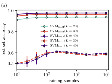
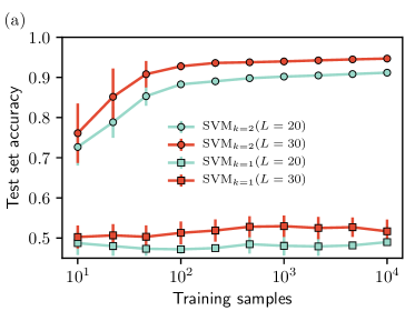
In order to quantify the performance of each SVM model, the main metric that we study is the test set accuracy as a function of the number of samples in the training set, for the value of which results in the optimal accuracy of the model, illustrated in Fig. 1 (a). For the linear kernel, the exploration of is over a log-spaced grid of 11 values from to . For the quadratic kernel the accuracy does not depend significantly on the choice of and thus we fixed it at . For a given number of training samples and regularization , the test set accuracy is additionally averaged over different random selections of training and test sets.
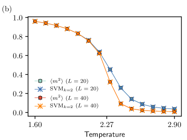
Results for the test set accuracy and for the SVM decision function are shown in Fig. 1. As seen in Fig. 1 (a), the quadratic kernel performs extremely well with mean test set accuracy for This can be easily interpreted, since we know that this model possesses a quadratic order parameter that linearly discriminates the FM from the PM, i.e. the squared magnetization per spin . We find that the quadratic kernel reaches very significant performance with only a few dozen samples in the training set, which is a result of the simplicity of this model. Moreover, with increasing number of samples the test set accuracy approaches a plateau value which increases with system size towards . This is the expected behaviour, since at the critical point the fluctuations of the order parameter approach zero in the thermodynamic limit and it is thus possible to discriminate perfectly between both phases.
For the linear kernel (Fig. 1 (a)), the accuracy shows non-monotonic behaviour with the total number of training set samples and does not improve with increasing system size. This is a consequence of the fact that a linear decision function is unable to discriminate between the FM and PM phases. Namely, in the FM phase configurations have magnetization per spin near , while for the PM phase most configurations have appproximately zero magnetization. Thus, the kernel is asking a linear decision boundary to separate a data set with three clusters – an impossible task. Close inspection of the decision function learned by the SVM reveals it contains random linear coefficients without any structure, confirming that nothing physically relevant is being learned about the data in this case.
As noted above, the accuracy of the SVM with a quadratic kernel on the test set does not depend significantly on the regularization parameter . An advantage of SVMs is that we can visualize the decision function being learned. From Eq. (2), the decision function for an SVM with quadratic polynomial kernel can be expressed as
| (3) |
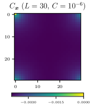
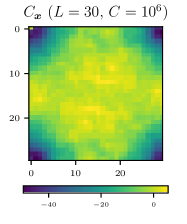
In Fig. 2, we display the heatmap of , where denotes averaging with respect to all sites for and and system size . It is interesting to note that even though the classification performance is very similar, the SVM decision function corresponds to different order parameters depending on the amount of regularization. Clearly, at , the SVM is learning as the order parameter of the model up to finite-size effects. In contrast, at , the SVM is learning to calculate the square of the total magnetization within some fixed distance of each spin and summing all these different local contributions. To further illustrate this point, in Fig. 1 (b), the SVM decision function (with regularization) is averaged over Monte Carlo samples at different temperatures showing essentially perfect agreement with . Of course, the SVM decision function has an arbitrary scale and off-set and in order to match with a linear transformation is performed, so that they agree at the extreme values of temperature and .
III.2 Conserved-order-parameter Ising model
The conserved-order-parameter Ising model Wang (2016) is described by the same Hamiltonian as the Ising model but the configuration space is restricted to the subspace where the total magnetization is zero. This model describes a half-filled lattice gas of particles with a nearest neighbour attractive interaction Newman and Barkema (1999). At low temperatures, domains of up and down spins are separated by either two horizontal or two vertical domain walls for a square lattice geometry with periodic boundary conditions. There is a phase transition to a featureless phase at the same critical temperature as the 2d Ising model. Ref. Wang (2016) studied this model on the square lattice using Principal Component Analysis (PCA), a dimensional reduction algorithm, and devised the following order parameter:
| (4) |
is of the form of Eq. (3) with
| (5) |
In contrast to PCA, which through feature dimension reduction provides the easy visualization required for the determination of this order parameter, SVMs should provide automated order parameter detection in a more systematic way. We explore this ability now.
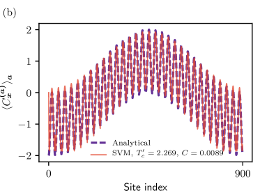
As in the case with the Ising model, we collect Monte Carlo samples for a set of temperatures below and above . Fig. 3 (a) shows the averaged test set accuracy as a function of the number of samples for the optimal value of the regularization parameter over a grid of 11 values from to . The results are averaged over training and test sets. As in the Ising model case, for a quadratic kernel there is a monotonic improvement of test accuracy with the number of training samples. The limiting value as the number of training samples becomes very large also increases with system size. This behavior signals the existence of a quadratic order parameter that discriminates between the two phases. As a check, we compare the explicit spatial dependence of the SVM decision function for (the selection of this regularization value is discussed below) to the analytical form (5). The scale and off-set of the SVM decision function are fixed by requiring the coefficients to have the same mean and standard deviation as the analytical form. Fig. 3 (b) shows very good agreement between them. In contrast, the linear kernel does not show a clear improvement of the test set accuracy with increasing number of samples which indicates there isn’t an order parameter of that form.
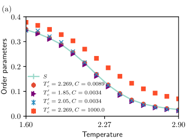
One could ask whether this order parameter could also be learned in the case where the precise value of the critical temperature is not known. We address this by performing supervised learning with quadratic SVMs assuming different values for the critical temperature. Finite-size scaling of the learned order parameter (or its moments) can then be used to estimate the value of the critical temperature. Fig. 4 (a) compares the actual order parameter (Eq. (4)) with the SVM decision function for different values of . The scale and off-set of the SVM decision function are fixed by matching it with at and . We observe that the SVM decision functions learned when assuming (for a choice of regularization values discussed below) also agree well with , suggesting machine learning algorithms are able to learn important physical information without the precise knowledge of .
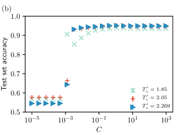
We now analyze the role of the regularization parameter for learning in this model. Fig. 4 (b), shows for and a training set with samples, the test set accuracy averaged over 10 randomly picked test sets of samples versus the regularization parameter for . At , the test set accuracy jumps significantly to very high values () and then reaches a plateau. Interestingly, we find that throughout the plateau region the decision function of the SVM changes continuously. Fig. 4 (a) also compares the analytical order parameter with the SVM decision function for different values of when . For , right at the beginning of the plateau, there is highly accurate agreement between and the SVM decision function, while for the two do not match. Similar results were also found for the other values of . Thus, the physical order parameter can be interpreted as being associated with the least amount of complexity that still allows the model to have good predictive performance. This was also what we found for the Ising model in Section III.1.
III.3 2d Ising Gauge theory
Finally, we consider the challenging case of topologically ordered systems, where no conventional local parameter exists. For concreteness we study the 2d Ising gauge theory with Hamiltonian , where the spins live on the bonds of a 2d square lattice and represents a plaquette with four spins. The set of ground states is a degenerate manifold with the constraint that for all plaquettes , . In the thermodynamic limit, the constraints are violated at any finite temperature. A conventional order parameter that distinguishes ground states from finite temperature states does not exist. Ref. Carrasquilla and Melko (2017) found that the simplest fully connected feed forward neural networks were unable to classify these two different cases in a supervised learning context. Only with convolutional neural networks, which explicitly exploit locality and translational invariance, did this classification task succeed on raw spin configurations. We note that by engineering predictive features as a pre-processing step, simple feed forward neural networks may be successful in classification (as demonstrated in Ref. Zhang and Kim (2016)). However in the present case, we explore the behaviour of SVMs for the raw 2d Ising Gauge theory data with no pre-processing on the input data.
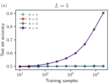
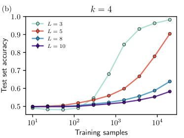
We perform supervised learning on spin configurations generated for the Ising Gauge theory at and (i.e. completely random spin states). We explore kernels of increasing degree, starting from , for different system sizes . Fig. 5 (a) shows that for system size , SVMs with polynomial kernel of degree less than 4 fail to discriminate these two phases, exhibiting average test set accuracies , which amounts to random guessing. However, a SVM with polynomial kernel of fourth order is able to perform the task with an accuracy that converges towards as the number of training samples is increased. As apparent in Fig. 5 (b), we also note that the number of training samples necessary to learn the fourth order discriminator increases with system size. This illustrates the difficulty that SVMs can have in performing classification for large system sizes.
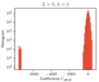
In order to interpret these results, we further analyze the decision function of the SVM. The smallest degree (fourth order) polymonial kernel learns a decision function of the form , which contains the product of four spins. Fig. 6 shows the histogram of the coefficients for an SVM trained on 20000 samples and . From this plot it is clear that there are two sets of coefficients; one near zero, and another set with large negative values. Counting the number of these large (in magnitude) coefficients reveals 600. For this lattice, with 25 square plaquettes, this number corresponds to the the number of possible permutations of the four indices of , i.e. . Hence, this model provides evidence that SVMs are able to learn complex interpretable decision functions and discover the locality of the Hamiltonian directly from raw data on spin configurations.
IV Conclusions
We have examined the use of support vector machines (SVMs), one of the most common tools for supervised learning, for the binary classification of phases in several models of interest to condensed matter and statistical physics. SVMs employ a kernel trick to define a decision function, used to discriminate features in a higher dimensional space. The kernel depends on the inner product of spin vectors, but can otherwise have some freedom in definition. We have shown that in contrast to other methods such as neural networks, the ability to use different kernels for classification tasks gives SVMs significant value in finding interpretable physical discriminators for different models, such as conventional order parameters defined in condensed matter theory.
To allow for some slack to misclassify data, SVMs employ a regularization, which controls the tradeoff between minimizing training errors, while still allowing sufficient model complexity. In this work we have found that the amount of regularization has a strong impact on the decision function learned. We find that the expected physical order parameter is associated with the least complex model (i.e. the largest amount of regularization) that is still able to obtain near-optimal test set accuracy.
On the other hand, we find that small values of regularization that achieve the same (or better) performance than the physical order parameter learn a non-physical decision function – one not related to any conventional order parameter. Since such decision functions generalize well to uncorrelated test set samples, we argue that this is not an example of overfitting, even though it may arise due to particular details contained within the training set. This observation deserves further study, as it may have consequences more generally for the role of regularization in black box algorithms, such as neural networks, when applied to data in condensed matter physics.
While very successful on the Ising-like examples studied in this paper, the SVM algorithm is not without its limitations. As observed for the 2d Ising Gauge Theory, the number of samples required to learn the physically-relevant decision function can grow prohibitively large. The reason that this occurs for the degenerate groundstate of the Ising gauge theory, and not the models with conventional order parameters, desires further study. We generally observe that the training of SVMs when the number of samples is larger than becomes time-consuming. This could also be an issue in using SVMs near phase transitions in models where a large number of samples is necessary to learn the physical discriminator. In such cases, it would be interesting to further explore the interpretability of neural networks, since they can possibly present better scalability to larger system sizes.
It would be interesting to study the utility of SVMs on other classical models of interest in condensed matter physics. We note that for systems with continuous degrees of freedom it might be necessary to consider a radial basis function as a kernel, which maps to an infinite dimensional space, instead of polynomials. For example, it would interesting to see if for the 2d XY model, the spin stiffness can be identified as the physical discriminator for the Kosterlitz-Thouless transition using a suitably-modified SVM. Finally, SVMs and other sparse kernel machines may in the future be easily adapted to study quantum phases and phase transitions by using wavefunctions or density matrices as data. SVMs with linear or quadratic polynomial kernels could be used to determine operators which discriminate between different quantum phases using density matrices or wavefunctions as data. Thus, as the condensed matter community increasingly adopts modern machine learning methods into its numerical arsenal, we expect that SVMs will become a standard tool for finding interpretable physical discriminators for generic Hamiltonians in the near future.
Acknowledgements – The authors thank Juan Carrasquilla for enlightening discussions. This research was supported by NSERC, the Canada Research Chair program, grant SFRH/BD/84875/2012 from Fundação para a Ciência e a Tecnologia (Portugal), and the Perimeter Institute for Theoretical Physics. Simulations were performed on resources provided by SHARCNET. Research at Perimeter Institute is supported through Industry Canada and by the Province of Ontario through the Ministry of Research & Innovation.
References
- Bishop (2006) C. M. Bishop, Pattern Recognition and Machine Learning (Springer-Verlag New York, Inc., Secaucus, NJ, USA, 2006).
- Murphy (2012) K. P. Murphy, Machine Learning: A Probabilistic Perspective (The MIT Press, 2012).
- Li et al. (2015) L. Li, J. C. Snyder, I. M. Pelaschier, J. Huang, U.-N. Niranjan, P. Duncan, M. Rupp, K.-R. Müller, and K. Burke, International Journal of Quantum Chemistry (2015).
- Carrasquilla and Melko (2017) J. Carrasquilla and R. G. Melko, Nat. Phys. http://dx.doi.org/10.1038/nphys4035 (2017).
- Wang (2016) L. Wang, Phys. Rev. B 94, 195105 (2016).
- Carleo and Troyer (2017) G. Carleo and M. Troyer, Science 355, 602 (2017).
- Torlai and Melko (2016a) G. Torlai and R. G. Melko, Phys. Rev. B 94, 165134 (2016a).
- Broecker et al. (2016) P. Broecker, J. Carrasquilla, R. G. Melko, and S. Trebst, arXiv preprint arXiv:1608.07848 (2016).
- Ch’ng et al. (2016) K. Ch’ng, J. Carrasquilla, R. G. Melko, and E. Khatami, arXiv preprint arXiv:1609.02552 (2016).
- Tanaka and Tomiya (2016) A. Tanaka and A. Tomiya, arXiv preprint arXiv:1609.09087 (2016).
- Ohtsuki and Ohtsuki (2016) T. Ohtsuki and T. Ohtsuki, Journal of the Physical Society of Japan 85, 123706 (2016).
- Li et al. (2016) L. Li, T. E. Baker, S. R. White, and K. Burke, Phys. Rev. B 94, 245129 (2016).
- Deng et al. (2016) D.-L. Deng, X. Li, and S. D. Sarma, arXiv preprint arXiv:1609.09060 (2016).
- Huang and Wang (2017) L. Huang and L. Wang, Physical Review B 95, 035105 (2017).
- Liu et al. (2017) J. Liu, Y. Qi, Z. Y. Meng, and L. Fu, Physical Review B 95, 041101 (2017).
- Torlai and Melko (2016b) G. Torlai and R. G. Melko, arXiv preprint arXiv:1610.04238 (2016b).
- van Nieuwenburg et al. (2017) E. P. L. van Nieuwenburg, Y.-H. Liu, and S. D. Huber, Nat. Phys. http://dx.doi.org/10.1038/nphys4037 (2017).
- Zhang and Kim (2016) Y. Zhang and E.-A. Kim, arXiv preprint arXiv:1611.01518 (2016).
- Portman and Tamblyn (2016) N. Portman and I. Tamblyn, arXiv preprint arXiv:1611.05891 (2016).
- Crawford et al. (2016) D. Crawford, A. Levit, N. Ghadermarzy, J. S. Oberoi, and P. Ronagh, arXiv preprint arXiv:1612.05695 (2016).
- Aoki and Kobayashi (2016) K.-I. Aoki and T. Kobayashi, Modern Physics Letters B , 1650401 (2016).
- Deng et al. (2017) D.-L. Deng, X. Li, and S. D. Sarma, arXiv preprint arXiv:1701.04844 (2017).
- Gao and Duan (2017) X. Gao and L.-M. Duan, arXiv preprint arXiv:1701.05039 (2017).
- Chen et al. (2017) J. Chen, S. Cheng, H. Xie, L. Wang, and T. Xiang, arXiv preprint arXiv:1701.04831 (2017).
- Huang and Moore (2017) Y. Huang and J. E. Moore, arXiv preprint arXiv:1701.06246 (2017).
- Wetzel (2017) S. J. Wetzel, arXiv preprint arXiv:1703.02435 (2017).
- Torlai et al. (2017) G. Torlai, G. Mazzola, J. Carrasquilla, M. Troyer, R. Melko, and G. Carleo, arXiv preprint arXiv:1703.05334 (2017).
- Hu et al. (2017) W. Hu, R. R. Singh, and R. T. Scalettar, arXiv preprint arXiv:1704.00080 (2017).
- Schindler et al. (2017) F. Schindler, N. Regnault, and T. Neupert, arXiv preprint arXiv:1704.01578 (2017).
- Pedregosa et al. (2011) F. Pedregosa, G. Varoquaux, A. Gramfort, V. Michel, B. Thirion, O. Grisel, M. Blondel, P. Prettenhofer, R. Weiss, V. Dubourg, J. Vanderplas, A. Passos, D. Cournapeau, M. Brucher, M. Perrot, and E. Duchesnay, Journal of Machine Learning Research 12, 2825 (2011).
- Platt (1998) J. Platt, in Advances in Kernel Methods - Support Vector Learning (MIT Press, 1998).
- Onsager (1944) L. Onsager, Phys. Rev. 65, 117 (1944).
- Newman and Barkema (1999) M. Newman and G. Barkema, Monte Carlo Methods in Statistical Physics (Oxford University Press, 1999).