$\bm{P}$-wave $\bm{\pi\pi}$ scattering and the $\bm{\rho}$ resonance from lattice QCD

Abstract

We calculate the parameters describing elastic $I=1$, $P$-wave $\pi\pi$ scattering using lattice QCD with $2+1$ flavors of clover fermions. Our calculation is performed with a pion mass of $m_{\pi}\approx 320\>\>{\rm MeV}$ and a lattice size of $L\approx 3.6$ fm. We construct the two-point correlation matrices with both quark-antiquark and two-hadron interpolating fields using a combination of smeared forward, sequential and stochastic propagators. The spectra in all relevant irreducible representations for total momenta $|\vec{P}|\leq\sqrt{3}\frac{2\pi}{L}$ are extracted with two alternative methods: a variational analysis as well as multi-exponential matrix fits. We perform an analysis using Lüscher’s formalism for the energies below the inelastic thresholds, and investigate several phase shift models, including possible nonresonant contributions. We find that our data are well described by the minimal Breit-Wigner form, with no statistically significant nonresonant component. In determining the $\rho$ resonance mass and coupling we compare two different approaches: fitting the individually extracted phase shifts versus fitting the $t$-matrix model directly to the energy spectrum. We find that both methods give consistent results, and at a pion mass of $am_{\pi}=0.18295(36)_{stat}$ obtain $g_{\rho\pi\pi}=5.69(13)_{stat}(16)_{sys}$, $am_{\rho}=0.4609(16)_{stat}(14)_{sys}$, and $am_{\rho}/am_{N}=0.7476(38)_{stat}(23)_{sys}$, where the first uncertainty is statistical and the second is the systematic uncertainty due to the choice of fit ranges.

I Introduction

One of the most fascinating phenomena of QCD is the hadronic spectrum: a complex set of composite particles arising from the interactions between quarks and gluons. If we neglect the electromagnetic and weak interactions, we can distinguish hadrons that are stable, i.e. those that do not decay via the strong interaction (for example the pion), and hadrons that are unstable, such as the $\rho$ meson.

The $\rho$ meson is an isotriplet of short-lived hadronic resonances with quantum numbers $J^{PC}=1^{--}$, which has been observed in multiple decay modes, including $\pi\pi$ (with a branching ratio of $99.9\%$), $\pi\pi\pi\pi$, $K\bar{K}$, and $\pi\gamma$ Olive:2016xmw . The two most important parameters of the $\rho$ meson are its resonant mass $m_{\rho}$ and its decay width $\Gamma_{\rho\to\pi\pi}$. Both have been studied extensively with lattice QCD Gottlieb:1985rc ; McNeile:2002fh ; Aoki:2007rd ; Gockeler:2008kc ; Jansen:2009hr ; Feng:2010es ; Frison:2010ws ; Lang:2011mn ; Aoki:2011yj ; Pelissier:2012pi ; Dudek:2012xn ; Wilson:2015dqa ; Bali:2015gji ; Bulava:2016mks ; Hu:2016shf ; Guo:2016zos ; Fu:2016itp , but many questions remain open, concerning for example the detailed dependence on the quark masses, the effects of $N_{f}=2+1$ versus $N_{f}=2$ sea quarks, the coupling to the $K\bar{K}$ channel, and the size of discretization errors for different lattice actions.

The $\rho$ resonance corresponds to a pole in the $I=1$ $P$-wave $\pi\pi$ scattering amplitude. This scattering amplitude plays an important role in many Standard Model processes, and its energy dependence must be determined accurately as part of lattice calculations of matrix elements involving the $\rho$ Briceno:2014uqa , such as $\pi\gamma\to\rho(\to\pi\pi)$ Briceno:2015dca ; Briceno:2016kkp and $B\to\rho(\to\pi\pi)\ell\bar{\nu}_{\ell}$.

In this work, we use the Lüscher method to study the $\rho$ resonance in $\pi\pi$ scattering with lattice QCD. The energy levels of a two-hadron system in a finite volume are shifted by the interactions between the hadrons. These energy shifts are related to the infinite-volume scattering matrix via the Lüscher quantization condition Luscher:1990ux . The Lüscher method was initially derived for the scattering of spin-$0$ particles in the rest frame Luscher:1990ux , and was extended to moving frames for the case of scattering of two particles with equal mass in Refs. Rummukainen:1995vs ; Kim:2005gf ; Christ:2005gi . Further generalizations to coupled channels, particles of unequal mass, arbitary spin, and three-particle systems were given in Refs. Hansen:2012tf ; Leskovec:2012gb ; Gockeler:2012yj ; Briceno:2014oea ; Briceno:2017tce . Other methods that have been used to study resonances are the Hamiltionian effective field theory approach Hall:2013qba , which is similar to the Lüscher method, the HALQCD approach HALQCD:2012aa , where the Nambu-Bethe-Salpeter wave function is calculated and used to determine a potential between two hadrons, and the method of Refs. McNeile:2002az ; Alexandrou:2013ata ; Alexandrou:2015hxa , which uses a perturbative interpretation of the mixing of nearby states.

We construct two-point correlation matrices with two different types of interpolating fields: quark-antiquark interpolators, and two-pion-scattering interpolators. From these correlation matrices, we extract the energy spectrum below the $K\bar{K}$ and $\pi\pi\pi\pi$ thresholds using two different analysis methods: 1) the variational approach, also known as the generalized eigenvalue problem, and 2), multi-exponential fits directly to the correlation matrix. We carefully compare the results from both methods and estimate the systematic uncertainties associated with the choice of the fit range.

In our Lüscher analysis of the elastic $\pi\pi$ scattering, we again compare two different methods: 1) mapping each individual energy level to a corresponding scattering phase shift, and then fitting Breit-Wigner-like models to the results, and 2) fitting the models for the $t$-matrix directly to the energy spectrum, as was proposed in Ref. Guo:2012hv . In constructing the models, we also allow for a possible nonresonant contribution.

Our calculation includes $N_{f}=2+1$ dynamical quark flavors, implemented with a clover-improved Wilson action. We use a single ensemble of gauge configurations on a $32^{3}\times 96$ lattice with $a\approx 0.114$ fm, corresponding to a large physical volume of $(3.6\>{\rm fm})^{3}\times(10.9\>{\rm fm})$. The calculation is performed in the isospin limit with a light-quark mass corresponding to a pion mass of approximately 320 MeV.

The paper is organized as follows: We begin by briefly reviewing the continuum description of elastic $\pi\pi$ scattering in Sec. II. Section III contains our lattice parameters and includes an analysis of the pion dispersion relation. Our choice of interpolating fields and the construction of the two-point correlation matrices are described in Sec. IV, and the analysis of the energy spectrum is reported in Sec. V. The formalism of the Lüscher analysis is reviewed in Sec. VI, while the numerical results for the scattering phase shifts and resonance parameters are discussed in Sec. VII.In Sec. VII we also present a detailed comparison with previous lattice calculations and discuss systematic uncertainties. We conclude in Sec. VIII.

II About $\pi\pi$ scattering

In this section we briefly review the formalism describing elastic $\pi\pi$ $P$-wave scattering in the $I(J^{PC})=1(1^{--})$ channel in the continuum Chung:1995dx .

We express the $1\times 1$ elastic scattering ’‘matrix” as

$$S_{\ell}(s)=1+2\mathrm{i}\;t_{\ell}(s),$$ (1)

where $t_{\ell}$ is the $t$-matrix (also known as the scattering amplitude), which depends on the invariant mass $s$ of the system, and $\ell$ is the partial wave of the scattering channel. The $t_{\ell}$ matrix is related to the scattering phase shift $\delta_{\ell}$ via

$$t_{\ell}(s)=\frac{1}{\cot{\delta_{\ell}(s)}-\mathrm{i}}.$$ (2)

A resonant contribution to $t_{\ell}(s)$ can be described by a Breit-Wigner (BW) form,

$$t_{\ell}(s)=\frac{\sqrt{s}\,\Gamma(s)}{m_{R}^{2}-s-\mathrm{i}\sqrt{s}\,\Gamma(s)},$$ (3)

which corresponds to the phase shift

$$\delta_{\ell}(s)=\arctan\frac{\sqrt{s}\,\Gamma(s)}{m_{R}^{2}-s}.$$ (4)

In this work, we consider two different forms for the $\ell=1$ decay width $\Gamma(s)$:

• BW I: $P$-wave decay width:

  $$\Gamma_{I}(s)=\frac{g_{\rho\pi\pi}^{2}}{6\pi}\frac{k^{3}}{s},$$ (5)

  where $g_{\rho\pi\pi}$ is the coupling between the $\pi\pi$ scattering channel and the $\rho$ resonance, and $k$ is the scattering momentum defined via $\sqrt{s}=2\sqrt{m_{\pi}^{2}+k^{2}}$. This form was used in most previous lattice QCD studies.

• BW II: $P$-wave decay width modified with Blatt-Weisskopf barrier factors VonHippel:1972fg :

  $$\Gamma_{II}(s)=\frac{g_{\rho\pi\pi}^{2}}{6\pi}\frac{k^{3}}{s}\>\frac{1+(k_{R}r_{0})^{2}}{1+(kr_{0})^{2}},$$ (6)

  where $k_{R}$ is the scattering momentum at the resonance position and $r_{0}$ is the radius of the centrifugal barrier.

In certain cases, for example in $P$-wave $N\pi$ scattering, the phase shift is known to receive both resonant and nonresonant (NR) contributions Long:2009wq . We also allow for this possibilty in our analysis of $\pi\pi$ scattering and write the full $P$-wave phase shift as

$$\delta_{1}(s)=\delta_{1}^{BW}(s)+\delta_{1}^{NR}(s).$$ (7)

We investigate three different models for a nonresonant background contribution $\delta_{1}^{NR}$:

• NR I: a constant nonresonant phase $A$:

  $$\delta_{1}^{NR}(s)=A.$$ (8)

• NR II: a nonresonant phase depending linearly on $s$:

  $$\delta_{1}^{NR}(s)=A+Bs,$$ (9)

  where $A$ and $B$ are free parameters.

• NR III: zeroth order nonresonant effective-range expansion (ERE):

  $$\delta_{1}^{NR}(s)=\mathrm{arccot}\frac{2a_{1}^{-1}}{\sqrt{s-s^{thres}}},$$ (10)

  where $a_{1}^{-1}$ is the inverse scattering length and $s^{thres}=4m_{\pi}^{2}$ is the $\pi\pi$ threshold invariant mass.

III Lattice parameters

III.1 Gauge Ensemble

The parameters of the lattice gauge-field ensemble are given in Table 1. The gluon action is a tadpole-improved tree-level Symanzik action Symanzik:1983pq ; Symanzik:1983dc ; Symanzik:1983gh ; Luscher:1985zq . We use the same clover-improved Wilson action Wilson:1974sk ; Sheikholeslami:1985ij for the sea and valence quarks. The gauge links in the fermion action are smeared using one level of stout smearing Morningstar:2003gk with staple weight $\rho=0.125$ (the smearing smoothes out short-distance fluctuations and alleviates instabilities associated with low quark masses). The lattice scale reported in Table 1 was determined from the $\Upsilon(2S)-\Upsilon(1S)$ splitting Davies:2009tsa ; Meinel:2010pv calculated with NRQCD Lepage:1992tx at the physical $b$-quark mass. The strange-quark mass is consistent with its physical value as indicated by the ’‘$\eta_{s}$” mass Davies:2009tsa ; Dowdall:2011wh .

	C13
$N_{L}^{3}\times N_{T}$	$32^{3}\times 96$
$\beta$	$6.1$
$N_{f}$	$2+1$
$c_{sw}$	$1.2493097$
$am_{u,d}$	$-0.285$
$am_{s}$	$-0.245$
$N_{config}$	$1041$
$a$ [fm]	$0.11403(77)$
$L$ [fm]	$3.649(25)$
$am_{\pi}$	$0.18295(36)$
$am_{N}$	$0.6165(23)$
$am_{\eta_{s}}$	$0.3882(19)$
$m_{\pi}L$	$5.865(32)$

Table 1: Details of the gauge-field ensemble. $N_{L}$ and $N_{T}$ denote the number of lattice points in the spatial and time directions. The lattice spacing, $a$, was determined using the $\Upsilon(2S)-\Upsilon(1S)$ splitting. The ensemble was generated with $N_{f}=2+1$ flavors of sea quarks with bare masses $am_{u,d}$ and $am_{s}$, which lead to the given values of $am_{\pi}$, $am_{N}$, and $am_{\eta_{s}}$. The $\eta_{s}$ is an artificial pseudoscalar $s\bar{s}$ meson that can be used to tune the strange-quark mass Davies:2009tsa ; Dowdall:2011wh . The uncertainties given here are statistical only.

III.2 The pion mass and dispersion relation

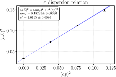
To determine the $\rho$ resonance parameters with the Lüscher method we need to know the pion dispersion relation. We performed a fit of the pion energies using the form $(aE)^{2}=(am_{\pi})^{2}+c^{2}(ap)^{2}$ in the range $0\leq p^{2}\leq 3(2\pi/L)^{2}$, which yields $am_{\pi}=0.18295(36)$ and $c^{2}=1.0195(86)$, as shown in Fig. 1. Given that $c^{2}$ is consistent with 1 within 2%, we use the relativistic dispersion relation $(aE)^{2}=(am_{\pi})^{2}+(ap)^{2}$ in the subsequent analysis.

Figure 1: Pion dispersion relation. The $\pi$ mass and speed of light determined from the dispersion relation are consistent with a relativistic dispersion relation with the rest frame $\pi$ energy.

IV Interpolating fields and two-point functions

The Lüscher quantization condition relates the infinite-volume $\pi\pi$ scattering phase shifts to the finite-volume energy spectrum Luscher:1990ux . The first step in our calculation is therefore to determine this energy spectrum from appropriate two-point correlation functions.

If there were no interactions between the two pions, the discrete energy levels of the two-pion system in a cubic lattice of size $L$ would be equal to

$$E_{non-int}^{\vec{P}}=\sqrt{m_{\pi}^{2}+|\vec{k}_{1}|^{2}}+\sqrt{m_{\pi}^{2}+|\vec{k}_{2}|^{2}},$$ (11)

where

$$\vec{k}_{1}=\frac{2\pi}{L}\vec{d}_{1},\;\;\vec{k}_{2}=\frac{2\pi}{L}\vec{d}_{2},\;\;\vec{d}_{1},\vec{d}_{2}\in{\mathbb{Z}}^{3},$$ (12)

and the total momentum is $\vec{P}=\vec{k}_{1}+\vec{k}_{2}$. In the presence of interactions, the individual momenta $\vec{k}_{1}$ and $\vec{k}_{2}$ are no longer good quantum numbers, but the total momentum still is, and takes on the values

$$\vec{P}=\frac{2\pi}{L}\vec{d},\;\;\vec{d}\in{\mathbb{Z}}^{3}.$$ (13)

We denote the interacting energy levels as

$$E_{n}^{\vec{P}},$$ (14)

where $n$ denotes the $n$-th state with the given total momentum (and any other relevant quantum numbers). We relate these energies to the corresponding center-of-mass energies

$$E_{n,\,CM}^{\vec{P}}=\sqrt{s_{n}^{\vec{P}}}=\sqrt{(E_{n}^{\vec{P}})^{2}-\vec{P}^{2}},$$ (15)

and define the scattering momentum $k_{n}^{\vec{P}}$ via

$$\sqrt{s_{n}^{\vec{P}}}=2\sqrt{m_{\pi}^{2}+(k_{n}^{\vec{P}})^{2}}.$$ (16)

Note that $k_{n}^{\vec{P}}$ is not a lattice momentum, and can take on continuous (possibly even imaginary) values. The interacting energy levels, and hence the scattering momenta, depend on the scattering phase shifts, the lattice size $L$, and the symmetries of the two-particle system, as described by the Lüscher quantization condition and its generalization to moving frames Luscher:1990ux ; Kim:2005gf ; Christ:2005gi .

We aim to determine the values of the scattering phase shift $\delta_{1}(s)$ for many values of $s$ near the $\rho$ resonance mass. The fairly large lattice volume we use ($L\approx 3.6$ fm) allows us to obtain a sufficient number of energy levels in the region of interest from only the single volume combined with multiple moving frames, $\vec{P}$. In this work, we use the moving frames and irreducible representations ($\Lambda$) listed in Table 2.

$\vec{P}$ $[\frac{2\pi}{L}]$	Little Group	Irrep $\Lambda$	$J$
$(0,0,0)$	$O_{h}$	$T_{1}^{-}$	$1^{-},3^{-},\ldots$
$(0,0,1)$	$D_{4h}$ (${\rm Dic}_{4}$)	$A_{2}^{-}$ ($A_{1}$)	$1^{-},3^{-},\ldots$
$(0,0,1)$	$D_{4h}$ (${\rm Dic}_{4}$)	$E^{-}$ ($E$)	$1^{-},3^{-},\ldots$
$(0,1,1)$	$D_{2h}$ (${\rm Dic}_{2}$)	$B_{1}^{-}$ ($A_{1}$)	$1^{-},3^{-},\ldots$
$(0,1,1)$	$D_{2h}$ (${\rm Dic}_{2}$)	$B_{2}^{-}$ ($B_{1}$)	$1^{-},3^{-},\ldots$
$(0,1,1)$	$D_{2h}$ (${\rm Dic}_{2}$)	$B_{3}^{-}$ ($B_{2}$)	$1^{-},3^{-},\ldots$
$(1,1,1)$	$D_{3d}$ (${\rm Dic}_{3}$)	$A_{2}^{-}$ ($A_{1}$)	$1^{-},3^{-},\ldots$
$(1,1,1)$	$D_{3d}$ (${\rm Dic}_{3}$)	$E^{-}$ ($E$)	$1^{-},3^{-},\ldots$

Table 2: The reference frames (i.e., total momenta $\vec{P}$), associated Little Groups, and irreducible representations used to determine the multi-hadron spectrum in the $I(J^{PC})=1(1^{--})$ channel. For the Little Groups and irreps with give both the Schönflies notation and the subduction notation. Due to a reduction in symmetry, the Little Group irreps $\Lambda$ contain not only $J^{P}=1^{-}$ states, but also higher $J$, starting with $J=3$. In the channel we investigate, the $J=3$ contributions have been shown to be negligible Estabrooks:1975cy ; Dudek:2012xn .

IV.1 Interpolating fields

The spectra in the frames and irreps listed in Table 2 are obtained from two-point correlation functions constructed using two different types of interpolating fields: local single-hadron quark-antiquark interpolating fields $\big{\{}O_{\bar{q}q}\big{\}}$, and two-hadron interpolating fields $\big{\{}O_{\pi\pi}\big{\}}$. We choose the quantum numbers $J^{PC}=1^{--}$ and $I=1,I_{3}=1$ (corresponding to the $\rho^{+}$ resonance), and write

$$O_{\bar{q}q}\big{(}t,\vec{P}\big{)} =\sum_{\vec{x}}\,\bar{d}(t,\vec{x})\,\Gamma\,u(t,\vec{x})\,\mathrm{e}^{\mathrm{i}\vec{P}\cdot\vec{x}}\,,$$ (17)

$$O_{\pi\pi}\big{(}t,\vec{p}_{1},\vec{p}_{2}\big{)} =\frac{1}{\sqrt{2}}\,\big{(}\pi^{+}(t,\vec{p}_{1})\,\pi^{0}(t,\vec{p}_{2})$$

$$\qquad-\pi^{0}(t,\vec{p}_{1})\,\pi^{+}(t,\vec{p}_{2})\big{)}\,,$$ (18)

where $\vec{P}=\vec{p}_{1}+\vec{p}_{2}$, and the single-pion interpolators are given by

$$\pi^{+}(t,\vec{p}) =\sum_{\vec{x}}\bar{d}(t,\vec{x})\,\gamma_{5}\,u(t,\vec{x})\,\mathrm{e}^{i\vec{p}\cdot\vec{x}}$$

$$\pi^{0}(t,\vec{p}) =\sum_{\vec{x}}\frac{1}{\sqrt{2}}\,\big{(}\bar{u}(t,\vec{x})\,\gamma_{5}\,u(t,\vec{x})$$

$$\qquad-\bar{d}(t,\vec{x})\,\gamma_{5}\,d(t,\vec{x})\big{)}\,\mathrm{e}^{i\vec{p}\cdot\vec{x}}\,.$$

We do not include quark-antiquark interpolators with derivatives, as past calculations have shown that such interpolators do not improve the determination of the spectrum near the $\rho$ resonance mass region Lang:2011mn .

In Eq. (17), we use two different $\Gamma_{i}$ matrices, namely $\gamma_{i}$ and $\gamma_{0}\gamma_{i}$, to obtain overlap with the $I(J^{PC})=1(1^{--})$ quantum numbers. The single-hadron interpolators are projected to the finite-volume irreps $\Lambda$ of the Little Group $LG(\vec{P})$ for the momentum $\vec{P}$ using

$$O_{\bar{q}q}^{\Lambda,\,\vec{P}}(t)=\frac{\mathrm{dim}(\Lambda)}{N_{LG(\vec{P})}}\sum_{\hat{R}\in LG(\vec{P})}\chi_{\Lambda}(\hat{R})\hat{R}\,O_{\bar{q}q}(t,\vec{P}),$$ (19)

where $\mathrm{dim}(\Lambda)$ is the dimension of the irrep, $N_{LG(\vec{P})}$ is the order of the Little Group, and $\chi_{\Lambda}(\hat{R})$ is the character of $\hat{R}\in LG(\vec{P})$ Dresselhaus:2008 .

The second interpolator type, Eq. (IV.1), is built from products of two single-pion interpolators, each separately projected to a definite momentum. In this case, the projection proceeds through the formula given in Ref. Feng:2010es :

$$O_{\pi\pi}^{\Lambda,\,\vec{P}}(t)=\frac{\mathrm{dim}(\Lambda)}{N_{LG(\vec{P})}}\sum_{\hat{R}\in LG(\vec{P})}$$ (20)

$$\chi_{\Lambda}(\hat{R})\bigg{(}\pi^{+}(t,\vec{P}/2+\hat{R}\vec{p}\,)\>\pi^{0}(t,\vec{P}/2-\hat{R}\vec{p}\,)$$ (21)

$$\hskip 12.91663pt-\pi^{0}(t,\vec{P}/2+\hat{R}\vec{p}\,)\>\pi^{+}(t,\vec{P}/2-\hat{R}\vec{p}\,)\bigg{)},$$ (22)

where

$$\vec{p}=\frac{\vec{P}}{2}+\frac{2\pi}{L}\vec{m},\;\;\vec{m}\in\mathbb{Z}^{3}.$$ (23)

(An alternative method to construct the interpolators is the subduction method Moore:2005dw ; Dudek:2012gj ; Prelovsek:2016iyo , which gives the same types of interpolators as we find with the projection method.)

In the following, we use the schematic notation $O_{1}$ for quark-antiquark interpolators with $\gamma_{i}$, $O_{2}$ for quark-antiquark interpolators with $\gamma_{0}\gamma_{i}$, and $O_{3}$, $O_{4}$ for two-pion interpolators with the smallest and second-smallest possible $\vec{p}$ in the given irrep.

IV.2 Wick contractions

The correlation matrix $C_{ij}^{\Lambda,\vec{P}}(t)$ is obtained from the interpolators defined above as

$$C_{ij}^{\Lambda,\vec{P}}(t_{f}-t_{i}) =\langle O_{i}^{\Lambda,\vec{P}}(t_{f})\>O_{j}^{\Lambda,\vec{P}}(t_{i})^{\dagger}\rangle\,,$$ (24)

where $t_{i}$ is the source time and $t_{f}$ is the sink time. The correlation matrix elements are expressed in terms of quark propagators by performing the Wick contractions (i.e., by performing the path integral over the quark fields in a given gauge-field configuration). The resulting quark-flow diagrams are shown in Fig. 2 (for the case $I=1$ considered here, further disconnected diagrams cancel due to exact isospin symmetry). In this section, we use the generic notation $\bar{q}q$ for the $i=1,2$ interpolators and $\pi\pi$ for the $i=3,4$ interpolators to describe our method.

Figure 2: The Wick contractions corresponding to the correlation matrix elements of type $C_{\bar{q}q-\bar{q}q}$, $C_{\pi\pi-\bar{q}q}$, $C^{\mathrm{direct}}_{\pi\pi-\pi\pi}$ and $C^{\mathrm{box}}_{\pi\pi-\pi\pi}$.

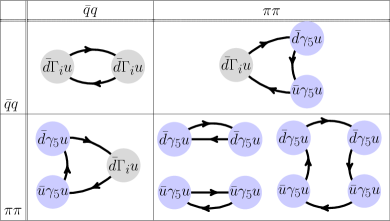
The diagrams in Fig. 2 are obtained from point-to-all propagators (labeled $f$), sequential propagators (labeled $seq$) and stochastic timeslice-to-all propagators (labeled $st$). In detail, these propagator types are given as follows:

a. Point-to-all propagator:

Writing the quark and anti-quark fields as $\psi(t_{f},\vec{x})_{\alpha}^{a}$ and $\bar{\psi}(t_{i},\vec{x}_{i})_{\beta}^{b}$, where $\alpha,\beta$ are spin indices and $a,b$ are color indices, the point-to-all propagator $S_{f}$ from the fixed initial point $x_{i}=(t_{i},\vec{x}_{i})$ to any final point $x_{f}=(t_{f},\vec{x}_{f})$ on the lattice is the matrix element of the inverse of the lattice Dirac operator $D$:

$$S_{f}(t_{f},\vec{x};t_{i},\vec{x}_{i})_{\alpha\beta}^{ab}=\langle\psi(t_{f},\vec{x}_{f})^{a}_{\alpha}\,\bar{\psi}(t_{i},\vec{x}_{i})^{b}_{\beta}\rangle_{f}$$

$$=D^{-1}(t_{f},\vec{x}_{f};t_{i},\vec{x}_{i})_{\alpha\beta}^{ab}\,.$$ (25)

b. Sequential propagator:

The sequential propagator describes the quark flow through a vertex of a given flavor and Lorentz structure. It is obtained from a point-to-all propagator by a second (sequential) inversion on a source built from the point-to-all propagator with an inserted vertex at timeslice $t_{seq}$ with spin structure $\Gamma$ and momentum insertion $\vec{p}$:

$$S_{seq}(t_{f},\vec{x}_{f};t_{seq},\vec{p},\Gamma;t_{i},\vec{x}_{i})$$

$$=\sum\limits_{\vec{x}_{seq}}\,D^{-1}(t_{f},\vec{x}_{f};t_{seq},\vec{x}_{seq})$$

$$\hskip 17.22217pt\times\,\Gamma\,\mathrm{e}^{i\vec{p}\cdot\vec{x}_{seq}}\,S_{f}(t_{seq},\vec{x}_{seq};t_{i},\vec{x}_{i})\,.$$ (26)

c. Stochastic timeslice-to-all propagator:

The stochastic timeslice-to-all propagator is defined as the inversion of the Dirac matrix with a stochastic timeslice momentum source:

$$S_{st}(t_{f},\vec{x}_{f};t_{i},\vec{x}_{i})=$$

$$\frac{1}{N_{\mathrm{sample}}}\,\sum\limits_{r=1}^{N_{\mathrm{sample}}}\,\phi^{r}_{t_{i},\vec{p}_{i}}(t_{f},\vec{x}_{f})\,\xi^{r}_{t_{i},\vec{0}}(t_{i},\vec{x}_{i})^{\dagger}\,,$$ (27)

where

$$\phi^{r}_{t_{i},\vec{p}_{i}} =D^{-1}\,\xi^{r}_{t_{i},\vec{p}_{i}}\,\mathrm{~{}and~{}}\xi^{r}_{t_{i},\vec{p}_{i}}(t,\vec{x})=\delta_{t,t_{i}}\,\mathrm{e}^{i\vec{p}_{i}\cdot\vec{x}}\,\xi^{r}_{t_{i}}(\vec{x})\,.$$

For each $r=1,\dotsc,N_{\mathrm{sample}}$, $\xi^{r}_{t_{i}}$ is a spin-color timeslice vector with independently distributed entries for real and imaginary part, $\xi^{r}_{t_{i}}(t,\vec{x})^{a}_{\alpha}\sim\mathbb{Z}_{2}\times i\mathbb{Z}_{2}$, so that the expectation values with respect to the stochastic noise, denoted as $\mathrm{E}\big{[}\quad\big{]}$, satisfy

$$\mathrm{E}\big{[}\xi^{r}_{t_{i}}(t,\vec{x})^{a}_{\alpha}\big{]}=0,$$ (28)

$$\mathrm{E}\big{[}\xi^{r_{1}}_{t_{i_{1}}}(\vec{x}_{1})^{a_{1}}_{\alpha_{1}}\,\big{(}\xi^{r_{2}}_{t_{i_{2}}}(\vec{x}_{2})^{a_{2}}_{\alpha_{2}}\big{)}^{*}\big{]}$$

$$=\delta^{r_{1},r_{2}}\,\delta_{t_{i_{1}},t_{i_{2}}}\,\delta_{\vec{x}_{1},\vec{x}_{2}}\,,\delta_{\alpha_{1},\alpha_{2}}\,\delta^{a_{1},a_{2}}\,.$$ (29)

This technique provides a good way to efficiently evaluate the box (and box-like) diagrams with reasonable cost. In addition to time-dilution of the stochastic momentum source, we also apply spin-dilution to make use of the efficient one-end-trick McNeile:2006bz in our contractions. In this case the stochastic sources read

$$\xi^{r}_{t_{i},\vec{p}_{i},\alpha}(t,\vec{x})^{b}_{\beta} =\delta_{t,t_{i}}\,\delta_{\alpha,\beta}\,\mathrm{e}^{i\vec{p}_{i}\cdot\vec{x}}\,\xi^{r}_{t_{i}}(\vec{x})^{b},$$ (30)

and the color timeslice vectors $\xi^{r}_{t_{i}}$ have expectation values analoguous to those in Eqs. (28) and (29).

d. Smearing:

To enhance the dominance of the lowest lying states contributing to a correlator we apply source and sink smearing to the propagator types listed above: for all inversions of the Dirac matrix we replace $D^{-1}\to W\big{[}U_{\mathrm{APE}}\big{]}\,D^{-1}\,W\big{[}U_{\mathrm{APE}}\big{]}^{\dagger}$, where $W\big{[}U_{\mathrm{APE}}\big{]}$ denotes the Wuppertal-smearing operator Gusken:1989ad using an APE-smeared gauge field Albanese:1987ds with the parameters $n=25$, $\alpha_{APE}=2.5$. Since the source and sink smearing is always understood, we will not denote it explicitly.

e. Coherent sequential sources:

In order to increase the available statistics for a fixed number of gauge configurations we calculate all correlators for 8 equidistant source locations separated in time by $T/8$ and with spatial source coordinates independently and uniformly sampled over the spatial lattice. We then take results from all source locations and average over them.

To reduce the computational cost for the sequential propagators, we insert 2 point-to-all propagators into a single sequential source before inverting the Dirac matrix on the latter:

$$S_{seq}=D^{-1}\,\xi_{seq},$$ (31)

$$\xi_{seq}(t,\vec{x})=\Gamma\,\mathrm{e}^{i\vec{p}\cdot\vec{x}}\,\bigg{(}\delta_{t,t^{(0)}_{i}}\,S_{f}\big{(}t^{(0)}_{i},\vec{x};t^{(0)}_{i},\vec{x}_{i}\big{)}$$

$$+\delta_{t,t^{(1)}_{i}}\,S_{f}\big{(}t^{(1)}_{i},\vec{x};t^{(1)}_{i},\vec{x}_{i}\big{)}\bigg{)},$$ (32)

where $t^{(1)}_{i}=t^{(0)}_{i}+T/2\mathrm{~{}mod~{}}T$.

The correlation matrix is then built from the propagators listed above as follows:

a. $\bar{q}q-\bar{q}q$ correlators:

The typical 2-point correlator with a single-hadron interpolator at source and sink is constructed using point-to-all propagators:

$$C_{\bar{q}q-\bar{q}q}(t_{f}-t_{i};\vec{p}_{f},\Gamma_{f};\vec{p}_{i},\Gamma_{i})=$$

$$-\sum_{\vec{x}_{f}}\,\mathrm{Tr}\big{(}(\gamma_{5}\,S_{f}(t_{f},\vec{x}_{f};t_{i},\vec{x}_{i})\,\gamma_{5})^{\tilde{\dagger}}$$

$$\quad\times\Gamma_{f}\,S_{f}(t_{f},\vec{x}_{f};t_{i},\vec{x}_{i})\,\Gamma_{i}\big{)}\mathrm{e}^{i\vec{p}_{f}\cdot\vec{x}_{f}+i\vec{p}_{i}\cdot\vec{x}_{i}}\,.$$ (33)

Above, $(\quad)^{\tilde{\dagger}}$ denotes the Hermitian adjoint with respect to only spin-color indices. We use the convention $\vec{p}_{f}=-\vec{p}_{i}$.

The direct diagram of the $C_{\pi\pi-\pi\pi}$ correlation function is the product of two of the previous correlators with $\Gamma_{i}=\gamma_{5}=\Gamma_{f}$. However, translational invariance allows only one of the $\vec{x}_{i}$ to be fixed. To perform the sum over $\vec{x}_{i}$, we use the one-end-trick and define

$$C_{\bar{q}q-\bar{q}q,oet}(t_{f}-t_{i};\Gamma_{f},\vec{p}_{f};\Gamma_{i},\vec{p}_{i})=$$

$$-\sum\limits_{\alpha,\beta}\,\sum_{\vec{x}_{f}}(\Gamma_{i}\gamma_{5})_{\alpha\beta}\,\phi_{t_{i},0,\beta}(t_{f},\vec{x}_{f})^{\tilde{\dagger}}\,\gamma_{5}\,\Gamma_{f}$$

$$\qquad\times\phi_{t_{i},\vec{p}_{i},\alpha}(t_{f},\vec{x}_{f})\,\mathrm{e}^{i\vec{p}_{f}\cdot\vec{x}_{f}}\,,$$ (34)

where $\phi_{t_{i},0,\beta}$ and $\phi_{t_{i},\vec{p}_{i},\alpha}$ are the spin-diluted stochastic timeslice-to-all propagators from Eqs. (IV.2) and (30). The stochastic-sample index $r$ is suppressed for brevity.

b. $\pi\pi-\bar{q}q$ correlators:

The only contribution to the $I=1$ correlators with a two-pion interpolator at the source and a single-hadron interpolator at the sink reads

$$C_{\bar{q}q-\pi\pi}(t_{f}-t_{i};\Gamma_{f},\vec{p}_{f};\vec{p}_{i_{1}},\vec{p}_{i_{2}})=$$

$$-\sum\limits_{\vec{x}_{f}}\,\mathrm{Tr}\big{(}S_{f}(t_{f},\vec{x}_{f};t_{i},\vec{x}_{i_{1}})^{\tilde{\dagger}}\,\gamma_{5}\,\Gamma_{f}$$

$$\times S_{seq}(t_{f},\vec{x}_{f};t_{i},\vec{p}_{i_{2}};t_{i},\vec{x}_{i_{1}})\big{)}\,\mathrm{e}^{i\vec{p}_{f}\cdot\vec{x}_{f}+i\vec{p}_{i_{1}}\cdot\vec{x}_{i_{1}}}\,,$$ (35)

where $S_{seq}$ is the sequential propagator from Eq.(IV.2).

c. $\pi\pi-\pi\pi$ correlators:

The direct diagram in the lower right panel of Fig. 2 is obtained as the product of two $\bar{q}q-\bar{q}q$ correlators as

$$C^{\mathrm{direct}}_{\pi\pi-\pi\pi}(t_{f}-t_{i};\vec{p}_{f_{1}},\vec{p}_{f_{2}},\vec{p}_{i_{1}},\vec{p}_{i_{2}})$$

$$=C_{\bar{q}q-\bar{q}q}(t_{f}-t_{i};\gamma_{5},\vec{p}_{f_{1}};\gamma_{5},\vec{p}_{i_{1}})$$

$$\quad\;\times C_{\bar{q}q-\bar{q}q,oet}(t_{f}-t_{i};\gamma_{5},\vec{p}_{f_{2}};\gamma_{5},\vec{p}_{i_{2}})\,.$$ (36)

The box-type diagram in the lower right panel of Fig. 2 requires point-to-all, sequential, and stochastic propagators and is calculated in two steps:

$$C^{\mathrm{box}}_{\pi\pi-\pi\pi}(t_{f}-t_{i},\vec{p}_{f_{1}},\vec{p}_{f_{2}},\vec{p}_{i_{1}},\vec{p}_{i_{2}})=$$

$$-\frac{1}{N_{\mathrm{sample}}}\,\sum\limits_{r=1}^{N_{\mathrm{sample}}}\,\sum\limits_{\alpha,a}\,\eta^{r}_{\phi}\big{(}t_{f},t_{i};\vec{p}_{f_{1}};\vec{x}_{i_{1}}\big{)}^{a}_{\alpha}$$

$$\qquad\times\eta^{r}_{\xi}\big{(}t_{f},t_{i};\vec{p}_{f_{2}},\vec{p}_{i_{2}};\vec{x}_{i_{1}}\big{)}^{a}_{\alpha}\,\mathrm{e}^{i\vec{p}_{i_{1}}\cdot\vec{x}_{i_{1}}}\,,$$ (37)

where

$$\eta^{r}_{\xi}\big{(}t_{f},t_{i};\vec{p}_{f_{2}},\vec{p}_{i_{2}};\vec{x}_{i_{1}}\big{)}=\sum\limits_{\vec{x}_{f_{2}}}\,\xi^{r}_{t_{f}}(t_{f},\vec{x}_{f_{2}})^{\tilde{\dagger}}\,\gamma_{5}$$

$$\times S_{seq}\big{(}t_{f},\vec{x}_{f_{2}};t_{i},\vec{p}_{i_{2}};t_{i},\vec{x}_{i_{1}}\big{)}\,\mathrm{e}^{i\vec{p}_{f_{2}}\cdot\vec{x}_{f_{2}}}$$ (38)

and

$$\eta^{r}_{\phi}\big{(}t_{f},t_{i};\vec{p}_{f_{1}};\vec{x}_{i_{1}}\big{)}=\sum\limits_{\vec{x}_{f_{1}}}\,S_{f}(t_{f},\vec{x}_{f_{1}};t_{i},\vec{x}_{i_{1}})^{\tilde{\dagger}}$$

$$\times\phi^{r}_{t_{f},0}(t_{f},\vec{x}_{f_{1}})\,\mathrm{e}^{i\vec{p}_{f_{1}}\cdot\vec{x}_{f_{1}}}\,.$$ (39)

In Eqs. (IV.2), (IV.2) and (IV.2) we used $\gamma_{5}$-Hermiticity of the quark propagator as well as $\Gamma_{i_{1/2}}=\gamma_{5}=\Gamma_{f_{1/2}}$.

The $\pi\pi$-$\pi\pi$ elements of the correlation matrix are constructed as

$$C_{\pi\pi-\pi\pi}(t_{f}-t_{i};\vec{p}_{f_{1}},\vec{p}_{f_{2}},\vec{p}_{i_{1}},\vec{p}_{i_{2}})=$$

$$\qquad\frac{1}{2}\,C^{\mathrm{direct}}_{\pi\pi-\pi\pi}(t_{f}-t_{i};\vec{p}_{f_{1}},\vec{p}_{f_{2}},\vec{p}_{i_{1}},\vec{p}_{i_{2}})$$

$$\qquad-C^{\mathrm{box}}_{\pi\pi-\pi\pi}(t_{f}-t_{i};\vec{p}_{f_{1}},\vec{p}_{f_{2}},\vec{p}_{i_{1}},\vec{p}_{i_{2}}).$$ (40)

V Spectrum results

We extract the energy levels $E_{n}^{\Lambda,\,\vec{P}}$ from the correlation matrices using two alternative methods. The first method, discussed in Sec. V.1, is the variational analysis, also known as the generalized eigenvalue problem (GEVP). The second method, discussed in Sec. V.2, employs multi-exponential fits directly to the correlation matrix.

V.1 Variational analysis

$\frac{L}{2\pi}|\vec{P}|$	$\Lambda$	Basis	$n$	Fit range	$\frac{\chi^{2}}{{\rm dof}}$	$aE_{n}^{\Lambda,\,\vec{P}}$	$a\sqrt{s_{n}^{\Lambda,\,\vec{P}}}$	$\delta_{1}$ $[^{\circ}]$	Included
$0$	$T_{1}$	$O_{1234}$	$1$	$8$-$18$	$0.82$	$0.4588(16)(12)$	$0.4588(16)(12)$	$86.0(1.6)(1.2)$	Yes
$0$	$T_{1}$	$O_{1234}$	$2$	$8$-$18$	$0.66$	$0.5467(16)(9)$	$0.5467(16)(9)$	$166.5(2.1)(1.3)$	Yes
$0$	$T_{1}$	$O_{1234}$	$3$	$7$-$15$	$1.54$	$0.6713(41)(104)$	$0.6713(41)(104)$	$172.9(4.7)(168.1)$	No
$1$	$A_{2}$	$O_{1234}$	$1$	$8$-$18$	$0.61$	$0.44536(73)(23)$	$0.39974(82)(25)$	$2.81(25)(9)$	Yes
$1$	$A_{2}$	$O_{1234}$	$2$	$8$-$18$	$1.04$	$0.5124(20)(17)$	$0.4732(22)(18)$	$131.3(1.9)(1.6)$	Yes
$1$	$A_{2}$	$O_{1234}$	$3$	$9$-$16$	$0.69$	$0.5983(31)(37)$	$0.5652(33)(39)$	$6.1(7.1)(8.3)$	No
$1$	$E$	$O_{123}$	$1$	$8$-$18$	$1.43$	$0.5004(18)(14)$	$0.4603(20)(16)$	$93.7(1.7)(1.3)$	Yes
$1$	$E$	$O_{123}$	$2$	$8$-$17$	$1.37$	$0.6136(25)(24)$	$0.5813(27)(26)$	$166.3(2.8)(2.7)$	Yes
$\sqrt{2}$	$B1$	$O_{1234}$	$1$	$8$-$18$	$1.23$	$0.5041(13)(10)$	$0.4207(16)(12)$	$8.84(89)(68)$	Yes
$\sqrt{2}$	$B1$	$O_{1234}$	$2$	$8$-$17$	$1.09$	$0.5557(26)(27)$	$0.4814(30)(31)$	$144.9(2.3)(2.4)$	Yes
$\sqrt{2}$	$B2$	$O_{1234}$	$1$	$8$-$18$	$0.56$	$0.5189(15)(11)$	$0.4384(18)(13)$	$19.9(1.7)(1.2)$	Yes
$\sqrt{2}$	$B2$	$O_{1234}$	$2$	$8$-$18$	$1.18$	$0.5634(26)(23)$	$0.4902(30)(27)$	$152.0(2.6)(2.4)$	Yes
$\sqrt{2}$	$B2$	$O_{1234}$	$3$	$8$-$16$	$1.28$	$0.6717(40)(49)$	$0.6116(44)(54)$	$158(14)(17)$	No
$\sqrt{2}$	$B3$	$O_{1234}$	$1$	$9$-$18$	$0.97$	$0.5376(38)(34)$	$0.4603(45)(39)$	$99.1(3.5)(3.1)$	Yes
$\sqrt{2}$	$B3$	$O_{1234}$	$2$	$9$-$18$	$1.15$	$0.6573(43)(49)$	$0.5958(48)(54)$	$174(15)(172)$	No
$\sqrt{2}$	$B3$	$O_{1234}$	$3$	$8$-$14$	$0.82$	$0.6780(67)(88)$	$0.6185(74)(96)$	$167.0(5.6)(6.9)$	No
$\sqrt{3}$	$A2$	$O_{1234}$	$1$	$8$-$18$	$0.68$	$0.5538(35)(49)$	$0.4371(44)(62)$	$15.5(3.4)(4.8)$	Yes
$\sqrt{3}$	$A2$	$O_{1234}$	$2$	$8$-$16$	$1.41$	$0.5905(35)(39)$	$0.4827(43)(48)$	$149(11)(13)$	Yes
$\sqrt{3}$	$A2$	$O_{1234}$	$3$	$8$-$16$	$1.10$	$0.6093(49)(50)$	$0.5055(59)(60)$	$156.5(7.5)(14.4)$	No
$\sqrt{3}$	$E$	$O_{123}$	$1$	$8$-$16$	$0.71$	$0.5641(37)(41)$	$0.4501(47)(50)$	$44.4(5.0)(5.3)$	Yes
$\sqrt{3}$	$E$	$O_{123}$	$2$	$7$-$16$	$0.72$	$0.6195(33)(54)$	$0.5178(39)(64)$	$160.6(3.3)(5.4)$	Yes

Table 3: GEVP results for the energy levels. We set $t_{0}/a=3$ and use the one-exponential form in Eq. (42) to fit the principal correlators. Also shown are the corresponding center-of-mass energy $\sqrt{s_{n}^{\Lambda,\,\vec{P}}}$ and extracted phase shift $\delta_{1}\Big{(}\sqrt{s_{n}^{\Lambda,\,\vec{P}}}\>\Big{)}$. The last column indicates whether the energy level is used our global analysis of $\pi\pi$ scattering (see Sec. VII).

The generalized eigenvalue problem is defined as

$$C^{\Lambda,\vec{P}}_{ij}(t)u^{n}_{j}(t)=\lambda^{n}(t,t_{0})C^{\Lambda,\vec{P}}_{ij}(t_{0})u_{j}^{n}(t),$$ (41)

where $t_{0}$ is a reference time Michael:1985ne ; Luscher:1990ck ; Blossier:2009kd ; Orginos:2015tha . At large $t$, the eigenvalues $\lambda^{n}(t,t_{0})$, which are also referred to as principal correlators, behave as

$$\lambda^{n}(t,t_{0})=\mathrm{e}^{-E_{n}^{\Lambda,\vec{P}}(t-t_{0})}.$$ (42)

To determine the energies $E_{n}^{\Lambda,\vec{P}}$, we fit the eigenvalues either with the single-exponential form of Eq. (42) or with the two-exponential form

$$\lambda^{n}(t,t_{0})=(1-B)\mathrm{e}^{-E_{n}^{\Lambda,\vec{P}}(t-t_{0})}+B\mathrm{e}^{-E_{n}^{{}^{\prime}\Lambda,\vec{P}}(t-t_{0})},$$ (43)

which perturbatively includes a small pollution from higher-lying excited states with energies $E_{n}^{{}^{\prime}\Lambda,\vec{P}}$ Luscher:1990ck ; Blossier:2009kd . We checked the GEVP spectrum for $t_{0}/a\in[2,9]$ and found that the central values are independent of $t_{0}$ within statistical uncertainties. We set $t_{0}/a=3$ for our main analysis, which minimizes the overall statistical noise. The chosen fit types, fit ranges, corresponding $\chi^{2}$ values, the energies, and other derived quantities are presented in Table 3. The operator basis used is $O_{1234}$ in all irreps except $E$, where we only use $O_{123}$ because the energy level dominantly overlapping with $O_{4}$ is too far above the region of interest.

For each quantity $y$, the first uncertainty given is the statistical uncertainty, obtained from single-elimination jackknife. The second uncertainty is the systematic uncertainty, estimated using the prescription

$$\sigma^{sys}_{y}={max}\bigg{(}|y_{avg}^{\prime}-y_{avg}|,\sqrt{|\sigma_{y}^{\prime 2}-\sigma_{y}^{2}|}\bigg{)},$$ (44)

where $y_{avg}$ and $\sigma_{y}$ are the central value and statistical uncertainty for the chosen fit range specificed in Table 3, and $y_{avg}^{\prime}$, $\sigma_{y}^{\prime}$ are the central value and statistical uncertainty obtained with $t_{min}/a$ increased by $1$.

V.2 Matrix fit analysis

Figure 3: Sample matrix fit with $N_{states}=3$ for $|\vec{P}|=\frac{2\pi}{L},\Lambda=A_{2}$ in the range between $t_{min}/a=8$ and $t_{min}/a=20$.

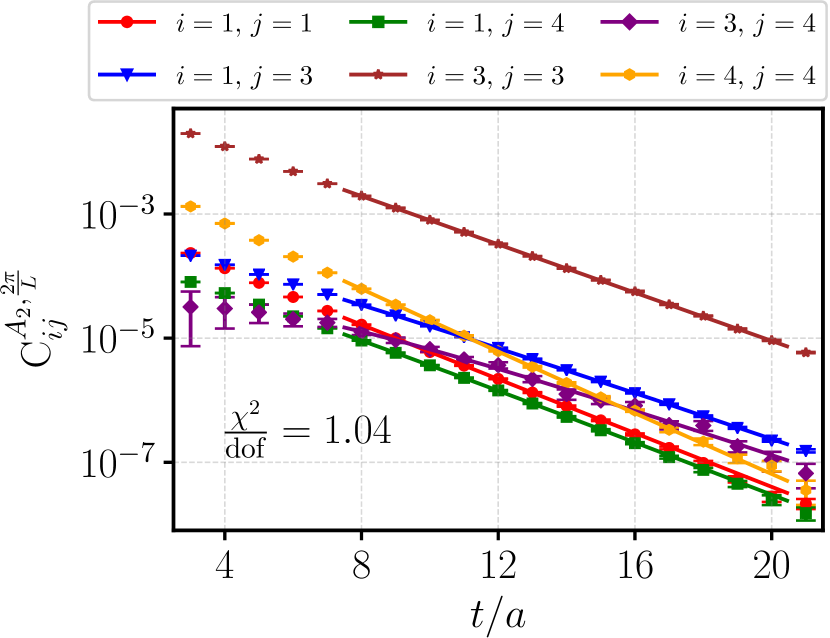
The spectral decomposition of the correlation matrix (neglecting the finite time extent of the lattice) reads

$$C^{\Lambda,\vec{P}}_{ij}(t)=\sum_{n=1}^{\infty}\langle 0|O_{i}|n,\Lambda,\vec{P}\rangle\>\langle n,\Lambda,\vec{P}|O_{j}^{\dagger}|0\rangle\>\mathrm{e}^{-E_{n}^{\Lambda,\vec{P}}t},$$ (45)

where $|n,\Lambda,\vec{P}\rangle$ is the $n$-th energy eigenstate with the given quantum numbers. We defined the interpolating fields $O_{i}$ such that the entire correlation matrix $C^{\Lambda,\vec{P}}_{ij}(t)$ is real-valued (in the infinite- statistics limit); this is possible because of charge-conjugation symmetry. Consequently, the overlap factors $Z_{i,\,n}=\langle 0|O_{i}|n,\Lambda,\vec{P}\rangle$ can also be chosen as real-valued. In the matrix fit analysis, we directly fit the correlation matrix for $t_{min}\leq t\leq t_{max}$ using the model

$$C^{\Lambda,\vec{P}}_{ij}(t) \approx \sum_{n=1}^{N_{states}}Z_{i,\,n}\>Z_{j,\,n}\>\mathrm{e}^{-E_{n}^{\Lambda,\vec{P}}t},$$ (46)

where $t_{min}$ has to be chosen large enough such that contributions from $n>N_{states}$ become negligible. For an $m\times m$ correlation matrix, this model has $N_{states}\times(m+1)$ parameters. To ensure that the energies returned from the fit are ordered, we used the logarithms of the energy differences, $l_{n}^{\Lambda,\vec{P}}=\ln\left(aE_{n}^{\Lambda,\vec{P}}-aE_{n-1}^{\Lambda,\vec{P}}\right)$, instead of $aE_{n}^{\Lambda,\vec{P}}$ (for $n>1$) as parameters in the fit. To simplify the task of finding suitable start values for the iterative $\chi^{2}$-minimization process, we also rewrote the overlap parameters as $Z_{i,\,n}=B_{i,\,n}Z_{i}$ with $B_{i,\,n}=1$ for $n$ equal to the state with which $O_{i}$ has the largest overlap. Good initial guesses for $Z_{i}$ can then be obtained from single-exponential fits of the form $Z_{i}Z_{i}\mathrm{e}^{-E_{n}^{\Lambda,\vec{P}}t}$ to the diagonal elements $C^{\Lambda,\vec{P}}_{ii}(t)$ in an intermediate time window in which the $n$-th state dominates, and the start values of $B_{i,\,n}$ can be set to zero. An example matrix fit is shown in Fig. 3.

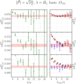
In the matrix fits, we excluded the interpolating fields $O_{2}$, which are very similar to $O_{1}$ and did not provide useful additional information. For each $(\Lambda,\vec{P})$, we performed either $3\times 3$ matrix fits (including $O_{1}$, $O_{3}$, $O_{4}$) with $N_{states}=3$ or $2\times 2$ matrix fits (including $O_{1}$ and $O_{3}$) with $N_{states}=2$. We set $t_{max}=20$ and varied $t_{min}.$ The matrix fit results for $aE_{n}^{\Lambda,\vec{P}}$ are shown as the black diamonds in the right panels of Figs. 4 and 5. We observe that the results for all extracted energy levels stabilize for $t_{min}\gtrsim 8$.

V.3 Comparison between GEVP and MFA

The results obtained from the GEVP and the MFA are compared in Figs. 4 and 5. The left panels show the effective energy

$$aE_{eff}^{n}(t)=\ln\frac{\lambda_{n}(t,t_{0})}{\lambda_{n}(t+a,t_{0})}$$ (47)

of the GEVP principal correlators, while the right panes show the fit results $aE^{n}_{fit}$ from both the GEVP and the MFA as a function of $t_{min}$ (we did not find any significant dependence on $t_{max}$). For the GEVP, we show both one- and two-exponential fits using Eqs. (42) and (43). We find that the one-exponential GEVP fit results are very similar (both in central value and uncertainty) to the MFA results, except for the $n=3$ energy level of the $|\vec{P}|=\sqrt{2}\frac{2\pi}{L},\Lambda=B_{1}$ correlation matrix where the principal correlator obtained from the GEVP with the basis $O_{1234}$ does not show a plateau and we do not extract this energy level. Surprisingly, we found that removing the second quark-antiquark operator $O_{2}$ from the basis yields a stable plateau and stable fit results for the $n=3$ energy level, as shown in Fig. 6. Note that $O_{2}\sim\bar{q}\gamma_{0}\gamma_{i}q$ has a very similar structure as $O_{1}\sim\bar{q}\gamma_{i}q$. For $n=1$ and $n=2$, the one-exponential fit results for the chosen $t_{\rm min}/a=8$ change by less than $0.5\sigma$ when removing $O_{2}$. We also performed additional GEVP fits with the reduced basis in all other irreps, and found that none of the fitted energies changed significantly (in fact, the reduced basis gives slightly larger uncertainties in most cases). Given that the $n=3$ energy in the $B_{1}$ irrep is above the $4\pi$ and $K\bar{K}$ thresholds, we do not use this energy level in our further analysis.

Figure 4: Comparison between MFA and GEVP for the momentum frames and irreps $\frac{L}{2\pi}|\vec{P}|=0,1,\sqrt{2}$ and $\Lambda=T_{1},A_{2},E,B_{1}$, respectively. The green circles on the left panel show the effective energies $E_{eff}^{n}$ determined from the principal correlators. In the right panel we present the fitted energies as they depend on the choice of $t_{min}$. Black diamonds are obtained from MFA, red squares are obtained from the single exponential fits to the principal correlator [see Eq. (42)], and blue circles are from two-exponential fits to the principal correlator [see Eq. (43)]. Note that not all two-exponential fits are shown, as they can become unstable. The red horizontal bands give the $1\sigma$ statistical-uncertainty ranges of the selected one-exponential GEVP fits listed in Table 3.

Figure 5: As in Fig. 4, but for $\frac{L}{2\pi}|\vec{P}|=\sqrt{2},\sqrt{3}$ and $\Lambda=B_{2},B_{3},A_{2},E$.

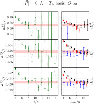
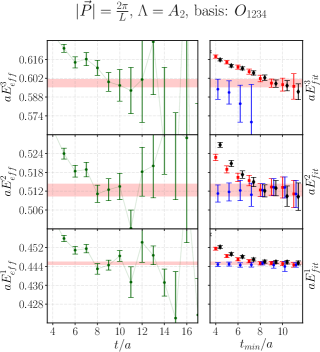
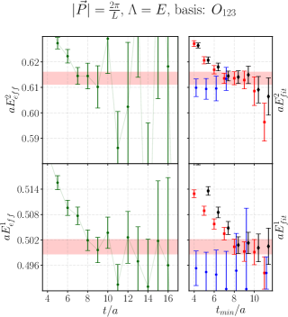
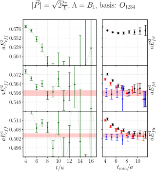
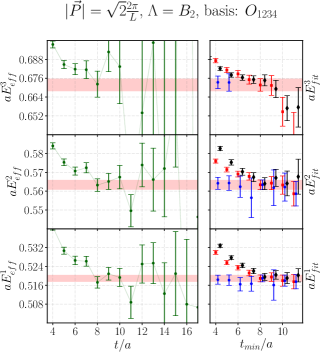
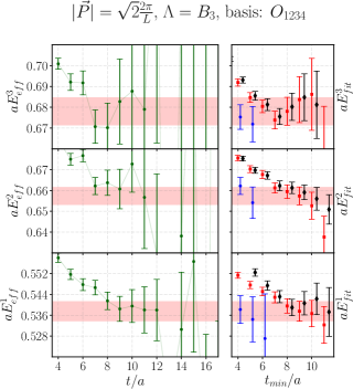
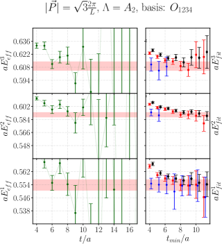
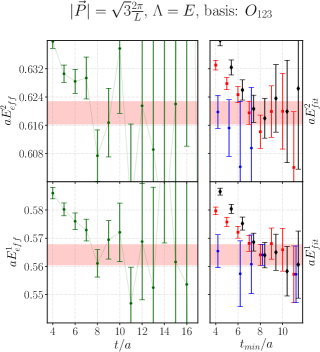
Finally, we note that the two-exponential fits to the GEVP principal correlators find plateaus at much smaller $t_{min}$ but are significantly noisier compared to the MFA and one-exponential GEVP fits. Overall, we have shown that the MFA and GEVP methods are equivalent, and we use the one-exponential GEVP fit results given in Table 3 in our further analysis. These results are also indicated with the red bands in Figs. 4 and 5.

Figure 6: Comparison between MFA and GEVP for the $B_{1}$ irrep with $|\vec{P}|=\sqrt{2}\frac{2\pi}{L}$ as in Fig. 4, but with $O_{2}$ removed from the basis for the GEVP. The reduced basis gives a better extraction of $aE_{3}$ compared to the full basis only in this irrep.

VI The Lüscher analysis: formalism

Even though we have some energy levels with quite large invariant mass (see Table 3), we limit our energy region of interest below $0.55a^{-1}$ where we are safely away from the $4\pi$ ($\approx 0.73$) and $K\bar{K}$ ($\approx 0.6$) thresholds Chen:2012rp and can safely perform the elastic scattering analysis of the Lüscher method.

The quantization condition for elastic $\pi\pi$ scattering is

$${\rm det}\bigg{(}\mathbbm{1}+\mathrm{i}t_{\ell}(s)(\mathbbm{1}+\mathrm{i}{\cal M}^{\vec{P}})\bigg{)}=0,$$ (48)

where $t_{\ell}(s)$ is the infinite-volume scattering amplitude, which is related to the infinite-volume scattering phase shift $\delta_{\ell}(s)$ via Eq. (2). The matrix ${\cal M}^{\vec{P}}$ has the indices ${\cal M}_{lm,l^{\prime}m^{\prime}}^{\vec{P}}$, where $l,l^{\prime}$ label the irreducible representations of $SO(3)$ and $m,m^{\prime}$ are the corresponding row indices. For the case of $P$-wave $\pi\pi$ scattering, $F$-wave and higher contributions are highly suppressed, as was shown in a previous lattice study Dudek:2012xn and in an analysis of experimental data Estabrooks:1975cy . Neglecting these contributions, the matrix ${\cal M}^{\vec{P}}$ takes the form

$${\cal M}^{\vec{P}}=\bordermatrix{~{}&0\,0&1\,0&1\,1&1\,-\!1\cr 0\>0&w_{00}&i\sqrt{3}w_{10}&i\sqrt{3}w_{11}&i\sqrt{3}w_{1-1}\cr 1\>0&-i\sqrt{3}w_{10}&w_{00}+2w_{20}&\sqrt{3}w_{21}&\sqrt{3}w_{2-1}\cr 1\>1&i\sqrt{3}w_{1-1}&-\sqrt{3}w_{2-1}&w_{00}-w_{20}&-\sqrt{6}w_{2-2}\cr 1\,-\!1&i\sqrt{3}w_{11}&-\sqrt{3}w_{21}&-\sqrt{6}w_{22}&w_{00}-w_{20}\cr},\$$ (49)

where the indices $lm$ and $l^{\prime}m^{\prime}$ are indicated next to the matrix. The functions $w_{lm}$ are equal to

$$w_{lm}^{\vec{P}}(k,L)=\frac{Z_{lm}^{\vec{P}}\left(1;(kL/(2\pi))^{2}\right)}{\pi^{3/2}\sqrt{2l+1}\gamma(\frac{kL}{2\pi})^{l+1}},$$ (50)

where $Z_{lm}^{\vec{P}}(1;(\frac{kL}{2\pi})^{2})$ is the generalized zeta function as defined for example in Appendix A of Ref. Leskovec:2012gb , and $\gamma=E/\sqrt{s}$ is the Lorentz boost factor. The matrix ${\cal M}^{\vec{P}}$ can be further simplified by taking into account the symmetries for a given Little Group ($\vec{P}$) and its irrep $\Lambda$ Leskovec:2012gb . The quantization condition (48) then reduces to the following equations for each $\vec{P}$ and $\Lambda$:

$$\vec{P}=0,\;\;\,\;\Lambda=T_{1}\text{: }$$

$$\;\cot{\delta_{1}(s_{n}^{\Lambda,\vec{P}})}=w_{0,0}\left(k_{n}^{\Lambda,\vec{P}},L\right)$$ (51)

$$\vec{P}=\frac{2\pi}{L}(0,0,1),\;\Lambda=A_{2}\text{: }$$ (52)

$$\;\cot{\delta_{1}(s_{n}^{\Lambda,\vec{P}})}=w_{0,0}\left(k_{n}^{\Lambda,\vec{P}},L\right)+2w_{2,0}\left(k_{n}^{\Lambda,\vec{P}},L\right)$$ (53)

$$\vec{P}=\frac{2\pi}{L}(0,0,1),\;\Lambda=E\text{: }$$ (54)

$$\;\cot{\delta_{1}(s_{n}^{\Lambda,\vec{P}})}=w_{0,0}\left(k_{n}^{\Lambda,\vec{P}},L\right)-w_{2,0}\left(k_{n}^{\Lambda,\vec{P}},L\right)$$ (55)

$$\vec{P}=\frac{2\pi}{L}(0,1,1),\;\Lambda=B_{1}\text{: }$$ (56)

$$\;\cot{\delta_{1}(s_{n}^{\Lambda,\vec{P}})}=w_{0,0}\left(k_{n}^{\Lambda,\vec{P}},L\right)+\frac{1}{2}w_{2,0}\left(k_{n}^{\Lambda,\vec{P}},L\right)+\mathrm{i}\sqrt{6}w_{2,1}\left(k_{n}^{\Lambda,\vec{P}},L\right)-\sqrt{\frac{3}{2}}w_{2,2}\left(k_{n}^{\Lambda,\vec{P}},L\right)$$ (57)

$$\vec{P}=\frac{2\pi}{L}(0,1,1),\;\Lambda=B_{2}\text{: }$$ (58)

$$\;\cot{\delta_{1}(s_{n}^{\Lambda,\vec{P}})}=w_{0,0}\left(k_{n}^{\Lambda,\vec{P}},L\right)+\frac{1}{2}w_{2,0}\left(k_{n}^{\Lambda,\vec{P}},L\right)-\mathrm{i}\sqrt{6}w_{2,1}\left(k_{n}^{\Lambda,\vec{P}},L\right)-\sqrt{\frac{3}{2}}w_{2,2}\left(k_{n}^{\Lambda,\vec{P}},L\right)$$ (59)

$$\vec{P}=\frac{2\pi}{L}(0,1,1),\;\Lambda=B_{3}\text{: }$$ (60)

$$\;\cot{\delta_{1}(s_{n}^{\Lambda,\vec{P}})}=w_{0,0}\left(k_{n}^{\Lambda,\vec{P}},L\right)-w_{2,0}\left(k_{n}^{\Lambda,\vec{P}},L\right)+\sqrt{6}w_{2,2}\left(k_{n}^{\Lambda,\vec{P}},L\right)$$

$$\vec{P}=\frac{2\pi}{L}(1,1,1),\;\Lambda=A_{2}\text{: }$$ (61)

$$\;\cot{\delta_{1}(s_{n}^{\Lambda,\vec{P}})}=w_{0,0}\left(k_{n}^{\Lambda,\vec{P}},L\right)-\mathrm{i}\sqrt{\frac{8}{3}}w_{2,2}\left(k_{n}^{\Lambda,\vec{P}},L\right)-\sqrt{\frac{8}{3}}\Bigg{(}{\rm Re}\left[w_{2,1}\left(k_{n}^{\Lambda,\vec{P}},L\right)\right]+{\rm Im}\left[w_{2,1}\left(k_{n}^{\Lambda,\vec{P}},L\right)\right]\Bigg{)}$$ (62)

$$\vec{P}=\frac{2\pi}{L}(1,1,1),\;\Lambda=E\text{: }$$ (63)

$$\;\cot{\delta_{1}(s_{n}^{\Lambda,\vec{P}})}=w_{0,0}\left(k_{n}^{\Lambda,\vec{P}},L\right)+\mathrm{i}\sqrt{6}w_{2,2}\left(k_{n}^{\Lambda,\vec{P}},L\right).$$ (64)

The scattering analysis can be performed in two different ways, and in this work we present a comparison between the methods:

• In the first approach, Eqs. (64) are used to map each individual energy level ($s_{n}^{\Lambda,\vec{P}}$) to the corresponding value of the scattering phase shift $\delta_{1}(s_{n}^{\Lambda,\vec{P}})$. One then fits a phase-shift model to the extracted values of $\delta_{1}(s_{n}^{\Lambda,\vec{P}})$.

• In the second approach, a model for the $t$-matrix is fitted directly to the spectrum via the quantization condition Guo:2012hv . This method has proven to be quite successful in recent years Dudek:2012gj ; Dudek:2012xn ; Dudek:2014qha ; Wilson:2014cna ; Wilson:2015dqa ; Dudek:2016cru ; Briceno:2016mjc . Unlike the first approach, the $t$-matrix fit method is also well-suited for more complicated coupled-channel analyses.

VII The Lüscher analysis: results

VII.1 Direct fits to the phases

Figure 7: Comparison of fitting Breit-Wigner model BW I versus fitting Breit-Wigner model BW II to the phase shift data. The bands indicate the $1\sigma$ statistical uncertainty.

Model	$\frac{\chi^{2}}{{\rm dof}}$	$am_{\rho}$	$g_{\rho\pi\pi}$	$(ar_{0})^{2}$
BW I	$0.571$	$0.4599(19)(13)$	$5.76(16)(12)$
BW II	$0.457$	$0.4600(18)(13)$	$5.79(16)(12)$	$8.6(8.0)(1.2)$

Table 4: Comparison of the parameters for the resonant Breit-Wigner models I and II.

Figure 8: Contribution of nonresonant background models as described in Section II to the resonant Breit-Wigner BW I. None of the background phase shift models shows a strong sign of deviation away from $0$.

Model	$\frac{\chi^{2}}{{\rm dof}}$	$am_{\rho}$	$g_{\rho\pi\pi}$
NR I	$0.586$	$0.4600(19)(13)$	$5.74(17)(14)$	$A=0.16(31)(18)^{\circ}$
NR II	$0.488$	$0.4602(19)(13)$	$5.84(21)(20)$	$A=-2.9(2.7)(3.4)^{\circ}$	$a^{-2}B=19.2(16.6)(20.1)^{\circ}$
NR III	$0.552$	$0.4601(19)(13)$	$5.74(16)(13)$	$aa_{1}^{-1}=-19.8(27.4)(98.1)$

Table 5: Parameters of the phase shift model combining the resonant Breit-Wigner model BW I and various nonresonant models.

Figure 9: Contribution of nonresonant background models as described in Section II to the resonant Breit-Wigner model BW II. None of the background phase shift models shows a strong sign of deviation away from $0$.

Model	$\frac{\chi^{2}}{{\rm dof}}$	$am_{\rho}$	$g_{\rho\pi\pi}$	$(ar_{0})^{2}$
NR I	$0.470$	$0.4599(19)(26)$	$5.83(20)(21)$	$15.8(23.5)(1825.8)$	$A=-0.28(0.73)(12.56)^{\circ}$
NR II	$0.452$	$0.4596(20)(14)$	$5.77(21)(20)$	$107.0(440.9)(631.0)$	$A=1.3(4.5)(5.3)^{\circ}$	$a^{-2}B=-19.8(16.0)(17.0)^{\circ}$
NR III	$0.421$	$0.4595(18)(8)$	$5.78(20)(9)$	$109.7(128.7)(117.6)$	$aa_{1}^{-1}=2.4(1.7)(2.4)$

Table 6: Parameters of the phase shift model combining the resonant Breit-Wigner model BW II and various nonresonant models.

The discrete $P$-wave phase shifts determined for several $\vec{P},\Lambda$ are listed in Table 3 next to the invariant masses. The first uncertainty given is the statistical uncertainty determined using single-elimination jackknife. The second uncertainty given is the systematic uncertainty resulting from the choice of $t_{min}$ in the fits to the GEVP principal correlators; it is computed by repeating the extraction of $\delta$ with $t_{min}+a$, and then applying Eq. (44) to the two phase shift results.

We then fit the models described in Sec. II to the phase shift points.

To correctly estimate the uncertainties of the model parameters, we include the uncertainties in both $\sqrt{s}$ and $\delta_{1}$ in the construction of the $\chi^{2}$ function. To this end, we define

$$\chi^{2}=\sum_{\vec{P},\Lambda,n}\>\>\sum_{\vec{P}^{\prime},\Lambda^{\prime},n^{\prime}}\>\>\sum_{i\in\left\{\sqrt{s_{n}^{\Lambda,\vec{P}}},\>\>\delta_{1}(s_{n}^{\Lambda,\vec{P}})\right\}}\>\>\sum_{j\in\left\{\sqrt{s_{n^{\prime}}^{\Lambda^{\prime},\vec{P}^{\prime}}},\>\>\delta_{1}(s_{n^{\prime}}^{\Lambda^{\prime},\vec{P}^{\prime}})\right\}}(y_{i}^{avg}-f_{i})[C^{-1}]_{ij}(y_{j}^{avg}-f_{j}),$$ (65)

where $i$ and $j$ are generalized indices labeling both the data points for $\sqrt{s}$ and $\delta_{1}$. The covariance matrix $C$ is therefore a $2N\times 2N$ matrix, where $N=15$ is the total number of energy levels included in the fit (see the last column of Table 3). For $i$ corresponding to a $\sqrt{s}$ data point, the function $f_{i}$ is equal to a nuisance parameter $\sqrt{s_{n}^{\Lambda,\vec{P}}}$; for $i$ corresponding to a $\delta_{1}$ data point, the function $f_{i}$ is equal to the phase shift model evaluated at the corresponding $\sqrt{s_{n}^{\Lambda,\vec{P}}}$. The total number of parameters in the fit is thus equal to $N$ plus the number of parameters in the phase shift model.

When constructing the covariance matrix, we included the correlations between all invariant-mass values and the correlations between all phase-shift values. We found that the covariance matrix becomes ill-conditioned when including also the cross-correlations between $\sqrt{s}$ and $\delta_{1}$ as expected when dealing with fully correlated data. We therefore neglect these contributions in the evaluation of $\chi^{2}$. The cross-correlations are nevertheless accounted for in our estimates of the parameter uncertainties, which are obtained by jackknife resampling.

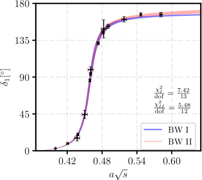
The fit of the simplest possible model, BW I, is shown as the blue curve in Fig. 7 and the resulting parameters $m_{\rho}$ and $g_{\rho\pi\pi}$ are given in the first row of Table 4. As before, the first uncertainty given is statistical, and the second uncertainty is the systematic uncertainty arising from the choice of $t_{min}$. To obtain the latter, we repeated the Breit-Wigner fit for the phase shifts extracted with $t_{min}+a$ for all energy levels, and then applied Eq. (44) to $m_{\rho}$ and $g_{\rho\pi\pi}$. We follow the same procedure for all other models.

We then investigate the effect of adding the Blatt-Weisskopf barrier factors VonHippel:1972fg to the decay width appearing in the Breit-Wigner parametrization of $\delta_{1}(s)$, which leads to model BW II. The resulting fit is shown as the red curve in Fig. 7 (alongside the blue BW I curve) and the resulting parameters are given in the second row of Table 4. The BW II model appears to give a slightly better description of the data at high invariant mass, but the paramaters $m_{\rho}$ and $g_{\rho\pi\pi}$ are essentially unchanged. Furthermore, the centrifugal barrier radius $r_{0}$ is consistent with zero at the $1.1\sigma$ level, indicating that it is not a very significant degree of freedom. We note that this could be related to the high pion mass used in our calculation, which limits the phase space available for the decay and suppresses the centrifugal barrier effect.

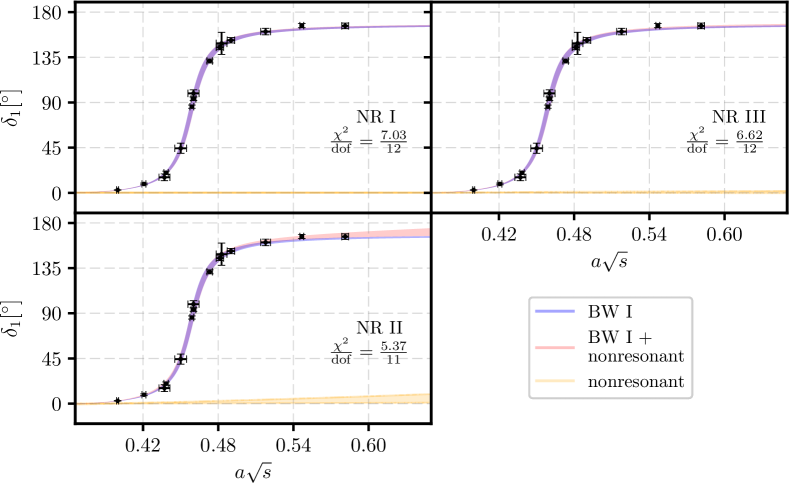
We continue by investigating whether there is a nonresonant contribution to the scattering phase shift. We first add a nonresonant contribution to the resonant model BW I. In Fig. 8 we compare the resonant-only fit (blue curve) with the full fits for three different forms of the nonresonant contributions (red curves). For clarity we also show the nonresonant contributions obtained from the full fits separately (orange curves). The fit results are given in Table 5. We find that the parameters of each of the three parametrizations NR I (constant phase), NR II (a nonresonant phase depending linearly on $s$), and NR III (zeroth-order ERE) are consistent with zero, and the results for $m_{\rho}$ and $g_{\rho\pi\pi}$ also do not change significantly.

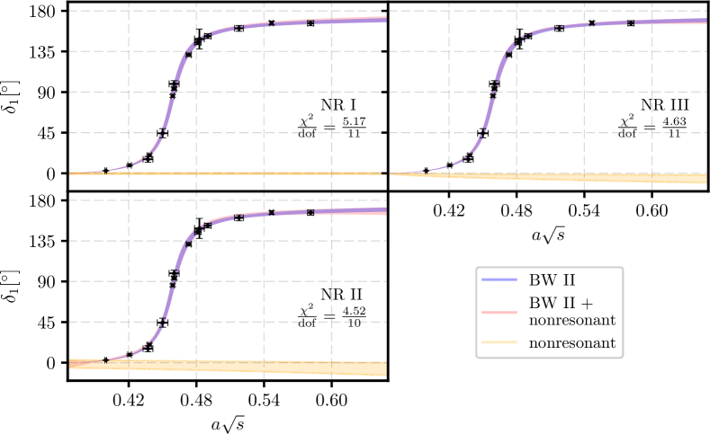
Performing the analoguous analysis for the resonant model BW II gives the phase shift curves shown in Fig. 9 and fit parameters in Table 6. Again, the parameters of the nonresonant contribution are consistent with zero, and $m_{\rho}$ and $g_{\rho\pi\pi}$ do not change significantly. When adding the nonresonant contributions to the BW II model, the uncertainty of the centrifugal barrier parameter $r_{0}$ increases substantially.

Overall, we find that the minimal resonant model BW I is sufficient for a good description of our results for the elastic $I=1$ $\pi\pi$ $P$-wave scattering.

VII.2 Fitting a $t$-matrix to the spectrum

Figure 10: Comparison of $t$-matrix fit and fit to the phase shifts for Breit-Wigner models I and II.

Fit type	$\frac{\chi^{2}}{{\rm dof}}$	$am_{\rho}$	$g_{\rho\pi\pi}$	$(ar_{0})^{2}$
BW I Fit to $\delta_{1}$	$0.571$	$0.4599(19)(13)$	$5.76(16)(12)$
BW I $t$-matrix fit	$0.374$	$0.4609(16)(14)$	$5.69(13)(16)$
BW II Fit to $\delta_{1}$	$0.457$	$0.4600(18)(13)$	$5.79(16)(12)$	$8.6(8.0)(1.2)$
BW II $t$-matrix fit	$0.318$	$0.4603(16)(14)$	$5.77(13)(13)$	$9.6(5.9)(3.7)$

Table 7: Comparison of $t$-matrix fits with direct fits to the phase shifts.

For the $t$-matrix fit to the spectrum, we define the $\chi^{2}$ function as

$$\chi^{2}=\sum_{\vec{P},\Lambda,n}\>\>\sum_{\vec{P}^{\prime},\Lambda^{\prime},n^{\prime}}\>\>\bigg{(}\sqrt{s_{n}^{\Lambda,\vec{P}}}^{[avg]}-\sqrt{s_{n}^{\Lambda,\vec{P}}}^{[model]}\bigg{)}[C^{-1}]_{\vec{P},\Lambda,n;\vec{P}^{\prime},\Lambda^{\prime},n^{\prime}}\bigg{(}\sqrt{s_{n^{\prime}}^{\Lambda^{\prime},\vec{P}^{\prime}}}^{[avg]}-\sqrt{s_{n^{\prime}}^{\Lambda^{\prime},\vec{P}^{\prime}}}^{[model]}\bigg{)},$$ (66)

where the invariant-mass values $\sqrt{s_{n^{\prime}}^{\Lambda^{\prime},\vec{P}^{\prime}}}^{[model]}$ are obtained by solving the inverse Lüscher problem, i.e. determining the finite-volume spectrum from a given $t$-matrix model Guo:2012hv ; Dudek:2012xn . Above, $C$ is the matrix of covariances between all invariant-mass values labeled by $\vec{P},\Lambda,n$ (in our case, this is a $15\times 15$ matrix). The only fit parameters in this approach are the parameters of the $t$ matrix (for example, $am_{\rho}$ and $g_{\rho\pi\pi}$ for the BW I model).

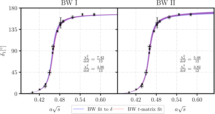
When fitting the $t$-matrix directly to the spectrum we consider only the two resonant models, as results from Sec. VII.1 show no indication of a nonresonant phase contribution. The parameters obtained from the $t$-matrix fits are compared to the parameters of the direct fits to the phase shifts in Table 7. The plots of the models with parameters from the two different fit approaches are compared in Fig. 10. The central values and uncertainties obtained with the two methods are consistent, which confirms previous findings Guo:2012hv ; Dudek:2012xn that the two approaches are equivalent not only theoretically but also in practice. We note that the values of $\chi^{2}/{\rm dof}$ are generally quite small. We have tested for the presence of autocorrelations in the data using binning, but found no significant effect.

VII.3 Final result for the $\rho$ resonance parameters

Figure 11: Final result of fitting the resonant model BW I to the spectrum via the $t$-matrix fit. The gray data points are the results of the individual phase shift extractions for each energy level, and are not used in the $t$-matrix fit.

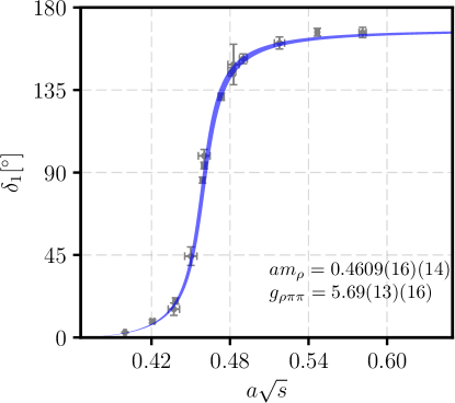
Given the discussion in the previous sections, we choose to quote the results of the $t$-matrix fit with the resonant Breit-Wigner model ${\bf BWI}$ as our final values of $am_{\rho}$ and $g_{\rho\pi\pi}$ for the ensemble of gauge configurations used here [with $am_{\pi}=0.18295(36)$ and $am_{N}=0.6165(23)$]:

$$\bordermatrix{&&&\cr am_{\rho}=0.4609(16)(14)&1.0&0.326\cr g_{\rho\pi\pi}=5.69(13)(16)&&1.0\cr}\ .$$ (67)

The phase shift curve of our chosen fit is shown in Fig. 11. Above, the first uncertainties given are statistical, and the second uncertainties are the systematic uncertainties related to the choice of $t_{min}$ in the spectrum analysis. Also given in Eq. (67) is the statistical correlation matrix for $am_{\rho}$ and $g_{\rho\pi\pi}$. The exponentially suppressed finite-volume errors in $m_{\rho}$ and $g_{\rho\pi\pi}$ are expected to be of order ${\cal O}(\mathrm{e}^{-m_{\pi}L})\approx 0.3\%$. Given that we have only one lattice spacing, we are unable to quantify discretization errors (except in the pion dispersion relation, Sec. III.2, where we find $c^{2}$ to be consistent with $1$ within $2\%$). Using the lattice spacing determined from the $\Upsilon(2S)-\Upsilon(1S)$ splitting (see Table 1), we obtain

$$m_{\pi} =316.6(0.6)_{stat}(2.1)_{a}\>\>{\rm MeV},$$

$$m_{\rho} =797.6(2.8)_{stat}(2.4)_{sys}(5.4)_{a}\>\>{\rm MeV},$$

$$g_{\rho\pi\pi} =5.69(13)_{stat}(16)_{sys}.$$ (68)

It is important to note that the lattice spacing uncertainty given here is statistical only. As a consequence of the heavier-than-physical pion mass and lattice artefacts, different quantities used to set the scale of an individual ensemble yield different results for $a$ and hence for $m_{\pi}$ and $m_{\rho}$ in units of MeV. We therefore prefer to report the dimensionless ratios

$$\frac{am_{\pi}}{am_{N}} =0.2968(13)_{stat},$$

$$\frac{am_{\rho}}{am_{N}} =0.7476(38)_{stat}(23)_{sys},$$ (69)

in which the lattice scale cancels.

In Fig. 12 we compare our results for the $\rho$ coupling and mass with the results of previous studies performed by the CP-PACS collaboration (CP-PACS ’07) Aoki:2007rd , the ETMC collaboration (ETMC ’10) Feng:2010es , the PACS-CS collaboration (PACS-CS ’11) Aoki:2011yj , Lang et al. (Lang et al. ’11) Lang:2011mn , the Hadron Spectrum collaboration (HadSpec ’12 and HadSpec ’15) Dudek:2012xn ; Wilson:2015dqa , Pellisier et al. (Pellisier et al. ’12) Pelissier:2012pi , the RQCD collaboration (RQCD ’15) Bali:2015gji , Guo et al. (Guo et al. ’16) Guo:2016zos , Bulava et al. (Bulava et al. ’16) Bulava:2016mks , and Fu et al. (Fu et al. ’16) Fu:2016itp . In the right half of the figure, we use the values of $m_{\pi}$ and $m_{\rho}$ in MeV as reported in each reference. In the left half of the figure, we instead use the dimensionless ratios $am_{\pi}/am_{N}$ and $am_{\rho}/am_{N}$, where $am_{\pi}$ and $am_{N}$ are the pion and nucleon masses in lattice units computed on the same ensemble as $am_{\rho}$. The nucleon masses were obtained from Refs. Namekawa:2004bi ; Alexandrou:2010hf ; Lin:2008pr ; Detmold:2015qwf ; Lang:2012db ; Aoki:2008sm ; Bali:2016lvx ; MILCmN .

We find that our value for the coupling $g_{\rho\pi\pi}$ is in good agreement with previous studies both as a function of $m_{\pi}$ and $am_{\pi}/am_{N}$. Furthermore, it is consistent with the general finding that $g_{\rho\pi\pi}$ has no discernible pion-mass dependence in the region between $m_{\pi,phys}$ and approximately $3\,m_{\pi,phys}$.

Figure 12: Comparison of our results for the $\rho$ mass and coupling with previous lattice QCD calculations. In the two left panels, we use the dimensionless ratios $am_{\rho}/am_{N}$ and $am_{\pi}/am_{N}$, while in the two right panels we use $m_{\pi}$ and $m_{\rho}$ in MeV as reported by each collaboration (with different scale setting methods; the error bars do not include the scale-setting ambiguities). The open red symbols mark calculations with $N_{f}=2$ gauge ensembles, while the filled blue symbols denote calculations with $N_{f}=2+1$ sea quarks; the only study so far that explicitly included the $K\bar{K}$ channel, HadSpec ’15, is presented as a purple upward facing triangle. The results of our present work are shown with filled black hexagons. In the left-hand plots, the HadSpec ’15 results are offset horizontally by $-1.8\%$ so that they do not overlap with the result of Bulava et al. ’16. In the right-hand plots, we offset our results by $-8\;{\rm MeV}$ to avoid overlap with Guo et al. ’16. The experimental values Olive:2016xmw , where $g_{\rho\pi\pi}$ was calculated from $\Gamma$ using Eq. (5), are shown with filled green circles.

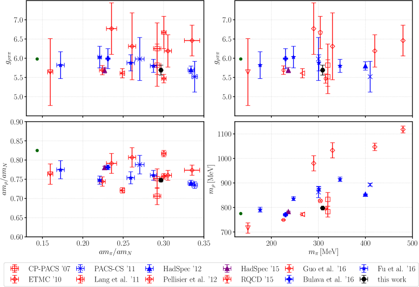
Concerning the results for the $\rho$ mass, the left and right panels of Fig. 12 show very different behavior. This discrepancy arises from the different methods used to set the lattice scale on a single ensemble, which can lead to misleading conclusions. To avoid the substantial ambiguities associated with the scale setting, we only consider the dimensionless ratio $am_{\rho}/am_{N}$ in the following discussion.

The $N_{f}=2+1$ results for $am_{\rho}/am_{N}$ obtained with Wilson-Clover-based fermion actions all approximately lie on a straight line leading to the experimental value (shown as the filled green circle in Fig. 12). The $N_{f}=2+1$ data points using staggered fermions (Fu et al. ’16) are consistent with that line except for one outlier.

The $N_{f}=2$ results are dispersed around the $N_{f}=2+1$ values in both directions. The discrepancies between the different results could arise from any of several systematic effects, such as excited-state contamination in the determination of the $\pi\pi$ spectrum or the nucleon mass, various potential issues in fitting the data, and discretization errors which manifest themselves for example in deviations from the relativistic continuum dispersion relation for the single-pion energies. Additionally, the Lüscher method only addresses power-law finite volume effects and does not take into account the exponentially suppressed finite-volume effects which are estimated to scale asymptotically as $O(e^{-m_{\pi}L})$. Note that for some of the studies, these can be as high as $O(10\%)$ and it is thus not clear whether the asymptotic regime is reached. An example for systematics associated with the pion dispersion relation can be seen in the CP-PACS ’07 study, where the two different results for $am_{\rho}$ at the same pion mass were obtained using either the relativistic continuum dispersion relation or a free-boson lattice dispersion relation. An example of systematic effects that might be associated with the data analysis can be seen when comparing the Pellisier et al. ’12 results with the Guo et al. ’16 results at $am_{\pi}/am_{N}\approx 0.3$. Both studies used the same ensemble, but arrive at significantly different values for the $\rho$ resonance parameters.

Keeping these caveats in mind, it is nevertheless interesting to note that our $N_{f}=2+1$ results for both $am_{\rho}/am_{N}$ and $g_{\rho\pi\pi}$ agree well with the recent $N_{f}=2$ results from Guo et al. ’16 at almost the same pion mass. This suggests that the effects of the dynamical strange quark are small at $m_{\pi}\approx 320$ MeV. The HadSpec ‘15 study, which explicitly included the $K\bar{K}$ channel in their valence sector, provides further evidence that the strange quark does not play a major role in the $\rho$ resonance mass.

VIII Summary and Conclusions

We have presented a $(2+1)$-flavor lattice QCD calculation of $I=1$, $P$ wave $\pi\pi$ scattering at a pion mass of approximately 320 MeV. The calculation was performed in a large volume of $(3.6\>{\rm fm})^{3}\times(10.9\>{\rm fm})$ and utilized all irreps of $LG(\vec{P})$ with total momenta up to $|\vec{P}|\leq\sqrt{3}\frac{2\pi}{L}$. Using a method based on forward, sequential, and stochastic propagators that scales well with the volume, we have achieved high statistical precision ($0.35\%$ for $am_{\rho}$ and $2.3\%$ for $g_{\rho\pi\pi}$).

We compared two different methods to determine the energy spectrum: the generalized eigenvalue problem (GEVP), and multi-exponential direct matrix fits to the correlation matrices (MFA). A careful investigation of the dependence on the fit ranges showed that both approaches are equally powerful and give consistent results.

After determining the elastic scattering phase shifts from the spectrum, we analyzed several different models for the energy dependence of the $\pi\pi$ scattering amplitude. We investigated two different Breit-Wigner forms, one with added Blatt-Weisskopf barrier factors, and found that the addition of this degree of freedom was not necessary to describe our data. This could be due to the higher-than-physical pion mass used in this work. Additionally, we examined whether there is a nonresonant contribution to the scattering phase shift, finding that it is consistent with zero within our statistical uncertainties.

Regarding the technical aspects of the analysis, we also compared two different ways of determining the scattering parameters: extracting the discrete phase shift points from each individual energy level (which is only feasible for elastic scattering) versus fitting the parameters of the $t$-matrix directly to the spectrum (as is also done in multichannel studies). We have demonstrated numerically that both methods are equivalent.

In summary, we found that the $I=1$, $P$-wave $\pi\pi$ scattering at $m_{\pi}\approx 320$ MeV is well described in the elastic energy region by the minimal resonant Breit-Wigner model BW I (defined in Sec. II) with the parameters given in Eq. (67). A comparison with previous lattice results, shown in Fig. 12, revealed that (i) it is important to use dimensionless ratios such as $am_{\rho}/am_{N}$ and $am_{\pi}/am_{N}$ to avoid scale setting ambiguities, and (ii) there are signs of significant systematic errors whose origins are difficult to disentangle without additional dedicated calculations.