CERN-TH-2017-086, IFUP-TH/2017 CP3-Origins-2017-014

Flavour anomalies after the RKsubscript𝑅superscript𝐾R_{K^{*}} measurement

(updated including the Moriond 2019 data from LHCb and Belle111The addendum at pages 6   Addendum: results presented at Moriond EW 20191 (section 6) is not present in the published version of this paper.)


Guido D’Amicoa, Marco Nardecchiaa, Paolo Pancia,
Francesco Sanninoa,b, Alessandro Strumiaa,c,
Riccardo Torred, Alfredo Urbanoa
a Theoretical Physics Department, CERN, Geneva, Switzerland
b CP3-Origins and Danish IAS, University of Southern Denmark, Denmark
c Dipartimento di Fisica dell’Università di Pisa and INFN, Italy
d Theoretical Particle Physics Laboratory, Institute of Physics, EPFL, Lausanne, Switzerland


Abstract

The LHCb measurement of the 𝝁/𝒆𝝁𝒆\mu/e ratio 𝑹𝑲subscript𝑹superscript𝑲R_{K^{*}} indicates a deficit with respect to the Standard Model prediction, supporting earlier hints of lepton universality violation observed in the 𝑹𝑲subscript𝑹𝑲R_{K} ratio. We show that the 𝑹𝑲subscript𝑹𝑲R_{K} and 𝑹𝑲subscript𝑹superscript𝑲R_{K^{*}} ratios alone constrain the chiralities of the states contributing to these anomalies, and we find deviations from the Standard Model at the 𝟒𝝈4𝝈4\sigma level. This conclusion is further corroborated by hints from the theoretically challenging 𝒃𝒔𝝁+𝝁bold-→𝒃𝒔superscript𝝁superscript𝝁b\to s\mu^{+}\mu^{-} distributions. Theoretical interpretations in terms of 𝒁superscript𝒁bold-′Z^{\prime}, lepto-quarks, loop mediators, and composite dynamics are discussed. We highlight their distinctive features in terms of the chirality and flavour structures relevant to the observed anomalies.

1 Introduction

The LHCb [1] collaboration presented their results on the measurement of the ratio

RK=BR(BKμ+μ)BR(BKe+e).subscript𝑅superscript𝐾BR𝐵superscript𝐾superscript𝜇superscript𝜇BR𝐵superscript𝐾superscript𝑒superscript𝑒R_{K^{*}}=\frac{\hbox{BR}(B\to K^{*}\mu^{+}\mu^{-})}{\hbox{BR}(B\to K^{*}e^{+}e^{-})}\,. (1)

The aim of this measurement is to test the universality of the gauge interactions in the lepton sector. Taking the ratio of branching ratios strongly reduces the Standard Model (SM) theoretical uncertainties, as suggested for the first time in ref. [2].

The experimental result [1] is reported in two bins of di-lepton invariant mass

RK={0.6600.070+0.110±0.024(2mμ)2<q2<1.1GeV20.6850.069+0.113±0.0471.1GeV2<q2<6GeV2.subscript𝑅superscript𝐾casesplus-or-minussubscriptsuperscript0.6600.1100.0700.024superscript2subscript𝑚𝜇2superscript𝑞21.1superscriptGeV2plus-or-minussubscriptsuperscript0.6850.1130.0690.0471.1superscriptGeV2superscript𝑞26superscriptGeV2R_{K^{*}}=\left\{\begin{array}[]{ll}0.660^{+0.110}_{-0.070}\pm 0.024&(2m_{\mu})^{2}<q^{2}<1.1\,{\rm GeV}^{2}\\[5.69054pt] 0.685^{+0.113}_{-0.069}\pm 0.047&1.1\,{\rm GeV}^{2}<q^{2}<6\,{\rm GeV}^{2}\,.\end{array}\right. (2)

These values have to be compared with the SM predictions [3]

RKSM={0.906±0.028(2mμ)2<q2<1.1GeV21.00±0.011.1GeV2<q2<6GeV2.subscriptsuperscript𝑅𝑆𝑀superscript𝐾casesplus-or-minus0.9060.028superscript2subscript𝑚𝜇2superscript𝑞21.1superscriptGeV2plus-or-minus1.000.011.1superscriptGeV2superscript𝑞26superscriptGeV2R^{SM}_{K^{*}}=\left\{\begin{array}[]{ll}0.906\pm 0.028&(2m_{\mu})^{2}<q^{2}<1.1\,{\rm GeV}^{2}\\[5.69054pt] 1.00\pm 0.01&1.1\,{\rm GeV}^{2}<q^{2}<6\,{\rm GeV}^{2}\,.\end{array}\right. (3)

At face value, a couple of observables featuring a 2.5σsimilar-toabsent2.5𝜎\sim 2.5\sigma deviation from the SM predictions can be attributed to a mere statistical fluctuation. The interest resides in the fact that such results might be part of a coherent picture involving New Physics (NP) in the bsμ+μ𝑏𝑠superscript𝜇superscript𝜇b\to s\mu^{+}\mu^{-} transitions. In fact, anomalous deviations were also observed in the following related measurements:

  1. 1.

    the RKsubscript𝑅𝐾R_{K} ratio [4]

    RK=BR(B+K+μ+μ)BR(B+K+e+e)=0.745±0.09stat±0.036syst;subscript𝑅𝐾BRsuperscript𝐵superscript𝐾superscript𝜇superscript𝜇BRsuperscript𝐵superscript𝐾superscript𝑒superscript𝑒plus-or-minus0.745subscript0.09statsubscript0.036systR_{K}=\frac{{\rm BR}\left(B^{+}\to K^{+}\mu^{+}\mu^{-}\right)}{{\rm BR}\left(B^{+}\to K^{+}e^{+}e^{-}\right)}=0.745\pm 0.09_{\rm stat}\pm 0.036_{\rm syst}\,; (4)
  2. 2.

    the branching ratios of the semi-leptonic decays BK()μ+μ𝐵superscript𝐾superscript𝜇superscript𝜇B\to K^{(*)}\mu^{+}\mu^{-} [5] and Bsϕμ+μsubscript𝐵𝑠italic-ϕsuperscript𝜇superscript𝜇B_{s}\to\phi\mu^{+}\mu^{-} [6];

  3. 3.

    the angular distributions of the decay rate of BKμ+μ𝐵superscript𝐾superscript𝜇superscript𝜇B\to K^{*}\mu^{+}\mu^{-}. In particular, the so-called P5subscriptsuperscript𝑃5P^{\prime}_{5} observable (defined for the first time in [7]) shows the most significant discrepancy [8, 5, 9].

The coherence of this pattern of deviations has been pointed out already after the measurement of RKsubscript𝑅𝐾R_{K} with a subset of observables in [10, 11] and in a full global analysis in [12, 13].

For the observables in points 222 and 333 the main source of uncertainty is theoretical. It resides in the proper evaluation of the form factors and in the estimate of the non-factorizable hadronic corrections. Recently, great theoretical effort went into the understanding of these aspects, see ref.s [14, 15, 7, 16, 17, 18, 19, 20, 21, 22, 23] for an incomplete list of references.

Given their reduced sensitivity to theoretical uncertainties in the SM, the RKsubscript𝑅𝐾R_{K} and RKsubscript𝑅superscript𝐾R_{K^{*}} observables offer a neat way to establish potential violation of lepton flavour universality. Future data will be able to further reduce the statistical uncertainty on these quantities. In addition, measurements of other ratios RHsubscript𝑅𝐻R_{H} analogous to RKsubscript𝑅𝐾R_{K}, with H=Xs,ϕ,K0(1430),f0𝐻subscript𝑋𝑠italic-ϕsubscript𝐾01430subscript𝑓0H=X_{s},\phi,K_{0}(1430),f_{0} will constitute relevant independent tests [2, 24].

The paper is structured as follows. In section 2 we discuss the relevant observables and how they are affected by additional effective operators. We perform a global fit in section 3. We show that, even restricting the analysis to the theoretically clean RKsubscript𝑅𝐾R_{K}, RKsubscript𝑅superscript𝐾R_{K^{*}} ratios, the overall deviation from the SM starts to be significant, at the 4σ4𝜎4\sigma level, and to point towards some model building directions. Such results prompt us to investigate, in section 4, a few theoretical interpretations. We discuss models including Zsuperscript𝑍Z^{\prime}, lepto-quark exchanges, new states affecting the observables via quantum corrections, and models of composite Higgs.

2 Effective operators and observables

Upon integrating out heavy degrees of freedom the relevant processes can be described, near the Fermi scale, in terms of the effective Lagrangian

eff=,X,YcbXY𝒪bXYsubscripteffsubscript𝑋𝑌subscript𝑐subscript𝑏𝑋subscript𝑌subscript𝒪subscript𝑏𝑋subscript𝑌\mathscr{L}_{\rm eff}=\sum_{\ell,X,Y}c_{b_{X}\ell_{Y}}{\cal O}_{b_{X}\ell_{Y}} (5)

where the sum runs over leptons ={e,μ,τ}𝑒𝜇𝜏\ell=\{e,\mu,\tau\} and over their chiralities X,Y={L,R}𝑋𝑌𝐿𝑅X,Y=\{L,R\}. New physics is more conveniently explored in the chiral basis

𝒪bXY=(s¯γμPXb)(¯γμPY).subscript𝒪subscript𝑏𝑋subscript𝑌¯𝑠subscript𝛾𝜇subscript𝑃𝑋𝑏¯subscript𝛾𝜇subscript𝑃𝑌{\cal O}_{b_{X}\ell_{Y}}=(\bar{s}\gamma_{\mu}P_{X}b)(\bar{\ell}\gamma_{\mu}P_{Y}\ell). (6)

These vector operators can be promoted to SU(2)LSUsubscript2𝐿\,{\rm SU}(2)_{L}-invariant operators, unlike scalar or tensor operators [25]. In SM computations one uses the equivalent formulation

eff=VtbVtsαem4πv2,X,YCbXY𝒪bXY+h.c.,formulae-sequencesubscripteffsubscript𝑉𝑡𝑏superscriptsubscript𝑉𝑡𝑠subscript𝛼em4𝜋superscript𝑣2subscript𝑋𝑌subscript𝐶subscript𝑏𝑋subscript𝑌subscript𝒪subscript𝑏𝑋subscript𝑌hc\mathscr{H}_{\rm eff}=-V_{tb}V_{ts}^{*}\frac{\alpha_{\rm em}}{4\pi v^{2}}\sum_{\ell,X,Y}C_{b_{X}\ell_{Y}}{\cal O}_{b_{X}\ell_{Y}}\,+\mathrm{h.c.}\,, (7)

defining dimensionless coefficients CIsubscript𝐶𝐼C_{I} as

cI=VtbVtsαem4πv2CI=CI(36TeV)2,subscript𝑐𝐼subscript𝑉𝑡𝑏superscriptsubscript𝑉𝑡𝑠subscript𝛼em4𝜋superscript𝑣2subscript𝐶𝐼subscript𝐶𝐼superscript36TeV2c_{I}=V_{tb}V_{ts}^{*}\frac{\alpha_{\rm em}}{4\pi v^{2}}C_{I}=-\frac{C_{I}}{(36\,{\rm TeV})^{2}}\,, (8)

where Vts=0.040±0.001subscript𝑉𝑡𝑠plus-or-minus0.0400.001V_{ts}=-0.040\pm 0.001 has a negligible imaginary part, v=174GeV𝑣174GeVv=174\,{\rm GeV} is the Higgs vacuum expectation value, usually written as 1/v2=4GF/21superscript𝑣24subscript𝐺F21/v^{2}=4G_{\rm F}/\sqrt{2}. The SM itself contributes as CbLLSM=8.64subscriptsuperscript𝐶SMsubscript𝑏𝐿subscript𝐿8.64C^{\rm SM}_{b_{L}\ell_{L}}=8.64 and CbLRSM=0.18subscriptsuperscript𝐶SMsubscript𝑏𝐿subscript𝑅0.18C^{\rm SM}_{b_{L}\ell_{R}}=-0.18, accidentally implying |CbLRSM||CbLLSM|much-less-thansubscriptsuperscript𝐶SMsubscript𝑏𝐿subscript𝑅subscriptsuperscript𝐶SMsubscript𝑏𝐿subscript𝐿|C^{\rm SM}_{b_{L}\ell_{R}}|\ll|C^{\rm SM}_{b_{L}\ell_{L}}|.

This observation suggests to use the chiral basis, related to the conventional one (see e.g. ref. [12]) by C9=CbLμL+R/2subscript𝐶9subscript𝐶subscript𝑏𝐿subscript𝜇𝐿𝑅2C_{9}=C_{b_{L}\mu_{L+R}}/2, C10=CbLμLR/2subscript𝐶10subscript𝐶subscript𝑏𝐿subscript𝜇𝐿𝑅2C_{10}=-C_{b_{L}\mu_{L-R}}/2, C9=CbRμL+R/2subscriptsuperscript𝐶9subscript𝐶subscript𝑏𝑅subscript𝜇𝐿𝑅2C^{\prime}_{9}=C_{b_{R}\mu_{L+R}}/2, C10=CbRμLR/2subscriptsuperscript𝐶10subscript𝐶subscript𝑏𝑅subscript𝜇𝐿𝑅2C^{\prime}_{10}=-C_{b_{R}\mu_{L-R}}/2, with the approximate relation C9SMC10SMsuperscriptsubscript𝐶9SMsuperscriptsubscript𝐶10SMC_{9}^{\rm SM}\approx-C_{10}^{\rm SM} holding in the SM. To make the notation more compact, we define CbL±RYCbLY±CbRYsubscript𝐶subscript𝑏plus-or-minus𝐿𝑅subscript𝑌plus-or-minussubscript𝐶subscript𝑏𝐿subscript𝑌subscript𝐶subscript𝑏𝑅subscript𝑌C_{b_{L\pm R}\ell_{Y}}\equiv C_{b_{L}\ell_{Y}}\pm C_{b_{R}\ell_{Y}} and CbL+RL±RCbLL+CbRL±CbLR±CbRRsubscript𝐶subscript𝑏𝐿𝑅subscriptplus-or-minus𝐿𝑅plus-or-minussubscript𝐶subscript𝑏𝐿subscript𝐿subscript𝐶subscript𝑏𝑅subscript𝐿subscript𝐶subscript𝑏𝐿subscript𝑅subscript𝐶subscript𝑏𝑅subscript𝑅C_{b_{L+R}\ell_{L\pm R}}\equiv C_{b_{L}\ell_{L}}+C_{b_{R}\ell_{L}}\pm C_{b_{L}\ell_{R}}\pm C_{b_{R}\ell_{R}}, and CbX(μe)YCbXμYCbXeYsubscript𝐶subscript𝑏𝑋subscript𝜇𝑒𝑌subscript𝐶subscript𝑏𝑋subscript𝜇𝑌subscript𝐶subscript𝑏𝑋subscript𝑒𝑌C_{b_{X}(\mu-e)_{Y}}\equiv C_{b_{X}\mu_{Y}}-C_{b_{X}e_{Y}}.

We now summarize the theoretically clean observables111By theoretically clean observables we mean those ones predicted in the SM with an error up to few percent., presenting both the full expressions and the ones in chiral-linear approximation. The latter is defined by neglecting |CbLRSM||CbLLSM|much-less-thansubscriptsuperscript𝐶SMsubscript𝑏𝐿subscript𝑅subscriptsuperscript𝐶SMsubscript𝑏𝐿subscript𝐿|C^{\rm SM}_{b_{L}\ell_{R}}|\ll|C^{\rm SM}_{b_{L}\ell_{L}}| and expanding each coefficient CIsubscript𝐶𝐼C_{I} at first order in the beyond-the-standard-model (BSM) contribution, CI=CISM+CIBSMsubscript𝐶𝐼subscriptsuperscript𝐶SM𝐼subscriptsuperscript𝐶BSM𝐼C_{I}=C^{\rm SM}_{I}+C^{\rm BSM}_{I}.

2.1 RKsubscript𝑅𝐾R_{K} revisited

The experimental analysis is made by binning the observable in the squared invariant mass of the lepton system q2(P+P+)2superscript𝑞2superscriptsubscript𝑃superscriptsubscript𝑃superscript2q^{2}\equiv(P_{\ell^{-}}+P_{\ell^{+}})^{2}. Writing the explicit q2superscript𝑞2q^{2}-dependence, we have

RK[qmin2,qmax2]qmin2qmax2𝑑q2𝑑Γ(B+K+μ+μ)/𝑑q2qmin2qmax2𝑑q2𝑑Γ(B+K+e+e)/𝑑q2.subscript𝑅𝐾superscriptsubscript𝑞min2superscriptsubscript𝑞max2superscriptsubscriptsuperscriptsubscript𝑞min2superscriptsubscript𝑞max2differential-dsuperscript𝑞2differential-dΓsuperscript𝐵superscript𝐾superscript𝜇superscript𝜇differential-dsuperscript𝑞2superscriptsubscriptsuperscriptsubscript𝑞min2superscriptsubscript𝑞max2differential-dsuperscript𝑞2differential-dΓsuperscript𝐵superscript𝐾superscript𝑒superscript𝑒differential-dsuperscript𝑞2R_{K}[q_{\rm min}^{2},q_{\rm max}^{2}]\equiv\frac{\int_{q_{\rm min}^{2}}^{q_{\rm max}^{2}}dq^{2}d\Gamma(B^{+}\to K^{+}\mu^{+}\mu^{-})/dq^{2}}{\int_{q_{\rm min}^{2}}^{q_{\rm max}^{2}}dq^{2}d\Gamma(B^{+}\to K^{+}e^{+}e^{-})/dq^{2}}\,. (9)

The experimental value cited in eq. (33) refers to RKRK[1GeV2,6GeV2]subscript𝑅𝐾subscript𝑅𝐾1superscriptGeV26superscriptGeV2R_{K}\equiv R_{K}[1~{}{\rm GeV}^{2},6~{}{\rm GeV}^{2}]. To simplify the notation, however, in the following we will omit the units in brackets. Neglecting SM contributions from the electromagnetic dipole operator, justified by the cut qmin2=1superscriptsubscript𝑞min21q_{\rm min}^{2}=1 GeV2, and non-factorizable contributions from the weak effective Hamiltonian,222In the limit of vanishing lepton masses the decay rate in eq. (9) takes the form [12] dΓ(B+K+μ+μ)dq2=GF2αem2|VtbVts|2210π5MB3λ3/2(MB2,MK2,q2)(|FV|2+|FA|2),𝑑Γsuperscript𝐵superscript𝐾superscript𝜇superscript𝜇𝑑superscript𝑞2superscriptsubscript𝐺F2superscriptsubscript𝛼em2superscriptsubscript𝑉𝑡𝑏superscriptsubscript𝑉𝑡𝑠2superscript210superscript𝜋5superscriptsubscript𝑀𝐵3superscript𝜆32superscriptsubscript𝑀𝐵2superscriptsubscript𝑀𝐾2superscript𝑞2superscriptsubscript𝐹𝑉2superscriptsubscript𝐹𝐴2\frac{d\Gamma(B^{+}\to K^{+}\mu^{+}\mu^{-})}{dq^{2}}=\frac{G_{\rm F}^{2}\alpha_{\rm em}^{2}|V_{tb}V_{ts}^{*}|^{2}}{2^{10}\pi^{5}M_{B}^{3}}\lambda^{3/2}(M_{B}^{2},M_{K}^{2},q^{2})\left(|F_{V}|^{2}+|F_{A}|^{2}\right)~{}, (10) where GFsubscript𝐺FG_{\rm F} is the Fermi constant, λ(a,b,c)a2+b2+c22(ab+bc+ac)𝜆𝑎𝑏𝑐superscript𝑎2superscript𝑏2superscript𝑐22𝑎𝑏𝑏𝑐𝑎𝑐\lambda(a,b,c)\equiv a^{2}+b^{2}+c^{2}-2(ab+bc+ac), MB5.279subscript𝑀𝐵5.279M_{B}\approx 5.279 GeV, MK0.494subscript𝑀𝐾0.494M_{K}\approx 0.494 GeV, |VtbVts|40.58×10³subscript𝑉𝑡𝑏superscriptsubscript𝑉𝑡𝑠40.58superscript103|V_{tb}V_{ts}^{*}|\approx 40.58\times 10^{-3}. Introducing the QCD form factors f+,T(q2)subscript𝑓𝑇superscript𝑞2f_{+,T}(q^{2}) we have FA(q2)subscript𝐹𝐴superscript𝑞2\displaystyle F_{A}(q^{2}) =\displaystyle= (C10+C10)f+(q2),subscript𝐶10superscriptsubscript𝐶10subscript𝑓superscript𝑞2\displaystyle\left(C_{10}+C_{10}^{\prime}\right)f_{+}(q^{2})~{}, (11) FV(q2)subscript𝐹𝑉superscript𝑞2\displaystyle F_{V}(q^{2}) =\displaystyle= (C9+C9)f+(q2)+2mbMB+MK(C7+C7)fT(q2)SMelectromagneticdipolecontribution+hK(q2)nonfactorizableterm.subscript𝐶9superscriptsubscript𝐶9subscript𝑓superscript𝑞2subscript2subscript𝑚𝑏subscript𝑀𝐵subscript𝑀𝐾subscript𝐶7superscriptsubscript𝐶7subscript𝑓𝑇superscript𝑞2SMelectromagneticdipolecontributionsubscriptsubscript𝐾superscript𝑞2nonfactorizableterm\displaystyle(C_{9}+C_{9}^{\prime})f_{+}(q^{2})+\underbrace{\frac{2m_{b}}{M_{B}+M_{K}}\left(C_{7}+C_{7}^{\prime}\right)f_{T}(q^{2})}_{\rm SM\,electromagnetic\,dipole\,contribution}+\underbrace{h_{K}(q^{2})}_{\rm non-factorizable\,term}~{}. (12) Notice that for simplicity we wrote the Wilson coefficient C9subscript𝐶9C_{9} omitting higher-order αssubscript𝛼𝑠\alpha_{s}-corrections [26]. Neglecting SM electromagnetic dipole contributions (encoded in the coefficients C7()superscriptsubscript𝐶7C_{7}^{(\prime)}), and non-factorizable corrections, eq. (13) follows from Eqs (9,10) by rotating the coefficients C9,10()superscriptsubscript𝐶910C_{9,10}^{(\prime)} on to the chiral basis. the theoretical prediction for RKsubscript𝑅𝐾R_{K} is

RK=|CbL+RμLR|2+|CbL+RμL+R|2|CbL+ReLR|2+|CbL+ReL+R|2.subscript𝑅𝐾superscriptsubscript𝐶subscript𝑏𝐿𝑅subscript𝜇𝐿𝑅2superscriptsubscript𝐶subscript𝑏𝐿𝑅subscript𝜇𝐿𝑅2superscriptsubscript𝐶subscript𝑏𝐿𝑅subscript𝑒𝐿𝑅2superscriptsubscript𝐶subscript𝑏𝐿𝑅subscript𝑒𝐿𝑅2R_{K}=\frac{|C_{b_{L+R}\mu_{L-R}}|^{2}+|C_{b_{L+R}\mu_{L+R}}|^{2}}{|C_{b_{L+R}e_{L-R}}|^{2}+|C_{b_{L+R}e_{L+R}}|^{2}}\ . (13)

This is a clean observable, meaning that it is not affected by large theoretical uncertainties, and its SM prediction is RK=1subscript𝑅𝐾1R_{K}=1. QED corrections give a small departure from unity which, however, does not exceed few percents [3]. However, it has to be noted that new physics which affects differently μ𝜇\mu and e𝑒e can induce theoretical errors, bringing back the issue of hadronic uncertainties.

In the chiral-linear approximation, RKsubscript𝑅𝐾R_{K} becomes

 RK1+2ReCbL+R(μe)LBSMCbLμLSM , RK1+2ReCbL+R(μe)LBSMCbLμLSM \fcolorbox{gray}{Gray}{~$\displaystyle R_K \simeq 1 +2 \frac{ \Re C^{\rm BSM}_{b_{L+R} (\mu-e)_{L}}}{C^{\rm SM}_{b_L \mu_L}}$~}\ , (14)

indicating that the dominant effect stems from couplings to left-handed leptons. Any chirality of quarks works, as long as it is not orthogonal to L+R𝐿𝑅L+R, namely unless quarks are axial.

It is important to notice that the approximation in eq. (14), although capturing the relevant physics, is not adequate for a careful phenomenological analysis. The same remark remains valid for the simplified expression proposed in ref. [24], expanded up to quadratic terms in new physics coefficients. The reason is that the expansion is controlled by the parameter CbXlYBSM/CbXlYSMsubscriptsuperscript𝐶BSMsubscript𝑏𝑋subscript𝑙𝑌subscriptsuperscript𝐶SMsubscript𝑏𝑋subscript𝑙𝑌C^{\rm BSM}_{b_{X}l_{Y}}/C^{\rm SM}_{b_{X}l_{Y}}, a number that is not always smaller than 111. This is particularly true in the presence of new physics in the electron sector in which — as we shall discuss in detail — large values of the Wilson coefficients are needed to explain the observed anomalies. For this reason, all the results presented in this paper make use of the full expressions for both RKsubscript𝑅𝐾R_{K} [12] and, as we shall discuss next, RKsubscript𝑅superscript𝐾R_{K^{*}}.

2.2 Anatomy of RKsubscript𝑅superscript𝐾R_{K^{*}}

Given that the Ksuperscript𝐾K^{*} has spin 1 and mass MK=892MeVsubscript𝑀superscript𝐾892MeVM_{K^{*}}=892\,{\rm MeV}, the theoretical prediction for the RKsubscript𝑅superscript𝐾R_{K^{*}} ratio given in eq. (1) is

RK=(1p)(|CbL+RμLR|2+|CbL+RμL+R|2)+p(|CbLRμLR|2+|CbLRμL+R|2)(1p)(|CbL+ReLR|2+|CbL+ReL+R|2)+p(|CbLReLR|2+|CbLReL+R|2)subscript𝑅superscript𝐾1𝑝superscriptsubscript𝐶subscript𝑏𝐿𝑅subscript𝜇𝐿𝑅2superscriptsubscript𝐶subscript𝑏𝐿𝑅subscript𝜇𝐿𝑅2𝑝superscriptsubscript𝐶subscript𝑏𝐿𝑅subscript𝜇𝐿𝑅2superscriptsubscript𝐶subscript𝑏𝐿𝑅subscript𝜇𝐿𝑅21𝑝superscriptsubscript𝐶subscript𝑏𝐿𝑅subscript𝑒𝐿𝑅2superscriptsubscript𝐶subscript𝑏𝐿𝑅subscript𝑒𝐿𝑅2𝑝superscriptsubscript𝐶subscript𝑏𝐿𝑅subscript𝑒𝐿𝑅2superscriptsubscript𝐶subscript𝑏𝐿𝑅subscript𝑒𝐿𝑅2R_{K^{*}}=\frac{(1-p)(|C_{b_{L+R}\mu_{L-R}}|^{2}+|C_{b_{L+R}\mu_{L+R}}|^{2})+p\left(|C_{b_{L-R}\mu_{L-R}}|^{2}+|C_{b_{L-R}\mu_{L+R}}|^{2}\right)}{(1-p)(|C_{b_{L+R}e_{L-R}}|^{2}+|C_{b_{L+R}e_{L+R}}|^{2})+p\left(|C_{b_{L-R}e_{L-R}}|^{2}+|C_{b_{L-R}e_{L+R}}|^{2}\right)} (15)

where p0.86𝑝0.86p\approx 0.86 is the “polarization fraction” [27, 28, 24], that is defined as

p=g0+gg0+g+g.𝑝subscript𝑔0subscript𝑔parallel-tosubscript𝑔0subscript𝑔parallel-tosubscript𝑔perpendicular-top=\frac{g_{0}+g_{\parallel}}{g_{0}+g_{\parallel}+g_{\perp}}\,. (16)

The gisubscript𝑔𝑖g_{i} are the contributions to the decay rate (integrated over the the intermediate bin) of the different helicities of the Ksuperscript𝐾K^{*}. The index i𝑖i distinguishes the various helicities: longitudinal (i=0𝑖0i=0), parallel (i=i=\parallel) and perpendicular (i=𝑖perpendicular-toi=\perp). In the chiral-linear limit the expression for RKsubscript𝑅superscript𝐾R_{K^{*}} simplifies to

 RKRK4pReCbR(μe)LBSMCbLμLSM , RKRK4pReCbR(μe)LBSMCbLμLSM \fcolorbox{gray}{Gray}{~$\displaystyle R_{K^*} \simeq R_K - 4p \frac{\Re C^{\rm BSM}_{b_R(\mu-e)_L}}{C^{\rm SM}_{b_L \mu_L}} $~}\ , (17)

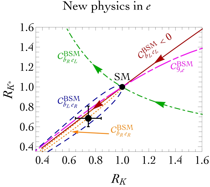
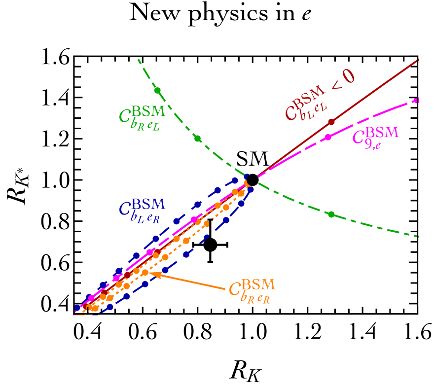
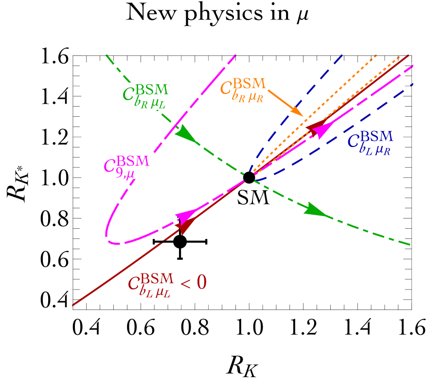
where 4p/CbLμLSM0.404𝑝subscriptsuperscript𝐶SMsubscript𝑏𝐿subscript𝜇𝐿0.404p/{C^{\rm SM}_{b_{L}\mu_{L}}}\approx 0.40. The formula above clearly shows that, in this approximation, a deviation of RKsubscript𝑅superscript𝐾R_{K^{*}} from RKsubscript𝑅𝐾R_{K} signals that bRsubscript𝑏𝑅b_{R} is involved at the effective operator level with the dominant effect still due to left-handed leptons. As already discussed before, eq. (17) is not suitable for a detailed phenomenological study, and we implement in our numerical code the full expression for RKsubscript𝑅superscript𝐾R_{K^{*}} [29]. In the left panel of figure 1, we present the different predictions in the (RK,RK)subscript𝑅𝐾subscript𝑅superscript𝐾(R_{K},R_{K^{*}}) plane due to turning on the various operators assumed to be generated via new physics in the muon sector. A reduction of the same order in both RKsubscript𝑅𝐾R_{K} and RKsubscript𝑅superscript𝐾R_{K^{*}} is possible in the presence of the left-handed operator CbLμLBSMsubscriptsuperscript𝐶BSMsubscript𝑏𝐿subscript𝜇𝐿C^{\rm BSM}_{b_{L}\mu_{L}} (red solid line). In order to illustrate the size of the required correction, the arrows correspond to CbLμLBSM=±1subscriptsuperscript𝐶BSMsubscript𝑏𝐿subscript𝜇𝐿plus-or-minus1C^{\rm BSM}_{b_{L}\mu_{L}}=\pm 1 (see caption for details). Conversely, as previously mentioned, a deviation of RKsubscript𝑅superscript𝐾R_{K^{*}} from RKsubscript𝑅𝐾R_{K} signals the presence of CbRμLBSMsubscriptsuperscript𝐶BSMsubscript𝑏𝑅subscript𝜇𝐿C^{\rm BSM}_{b_{R}\mu_{L}} (green dot-dashed line). Finally, notice that the reduced value of RKsubscript𝑅𝐾R_{K} measured in eq. (33) cannot be explained by CbRμRBSMsubscriptsuperscript𝐶BSMsubscript𝑏𝑅subscript𝜇𝑅C^{\rm BSM}_{b_{R}\mu_{R}} and CbLμRBSMsubscriptsuperscript𝐶BSMsubscript𝑏𝐿subscript𝜇𝑅C^{\rm BSM}_{b_{L}\mu_{R}}. The information summarized in this plot is of particular significance since it shows at a glance, and before an actual fit to the data, the new physics patterns implied by the combined measurement of RKsubscript𝑅𝐾R_{K} and RKsubscript𝑅superscript𝐾R_{K^{*}}.

Before proceeding, another important comment is in order. In the left panel of figure 1, we also show in magenta the direction described by non-zero values of the coefficient C9,μBSM=(CbLμLBSM+CbLμRBSM)/2subscriptsuperscript𝐶BSM9𝜇subscriptsuperscript𝐶BSMsubscript𝑏𝐿subscript𝜇𝐿subscriptsuperscript𝐶BSMsubscript𝑏𝐿subscript𝜇𝑅2C^{\rm BSM}_{9,\mu}=(C^{\rm BSM}_{b_{L}\mu_{L}}+C^{\rm BSM}_{b_{L}\mu_{R}})/2. The latter refers to the effective operator 𝒪9μ=(s¯γμPLb)(μ¯γμμ)superscriptsubscript𝒪9𝜇¯𝑠subscript𝛾𝜇subscript𝑃𝐿𝑏¯𝜇superscript𝛾𝜇𝜇\mathcal{O}_{9}^{\mu}=(\bar{s}\gamma_{\mu}P_{L}b)(\bar{\mu}\gamma^{\mu}\mu), and implies a vector coupling for the muon. The plot suggests that negative values C9,μBSM1subscriptsuperscript𝐶BSM9𝜇1C^{\rm BSM}_{9,\mu}\approx-1 may also provide a good fit of the observed data. However, it is also interesting to notice that in the non-clean observables, the hadronic effects might mimic a short distance BSM contribution in C9,μBSMsubscriptsuperscript𝐶BSM9𝜇C^{\rm BSM}_{9,\mu}. From the plot in our figure 1, it is clear that with more data a combined analysis of RKsubscript𝑅𝐾R_{K} and RKsubscript𝑅superscript𝐾R_{K^{*}} might start to discriminate between C9,μBSMsubscriptsuperscript𝐶BSM9𝜇C^{\rm BSM}_{9,\mu} and CbLμLBSMsubscriptsuperscript𝐶BSMsubscript𝑏𝐿subscript𝜇𝐿C^{\rm BSM}_{b_{L}\mu_{L}} using only clean observables. However, with the present data, there is only a mild preference for CbLμLBSMsubscriptsuperscript𝐶BSMsubscript𝑏𝐿subscript𝜇𝐿C^{\rm BSM}_{b_{L}\mu_{L}}, according to the 1-parameter fits of section 3.1 using only clean observables.

It is also instructive to summarise in the right panel of figure 1 the case in which new physics directly affects the electron sector. The result is a mirror-like image of the muon case since the coefficients CbXeYsubscript𝐶subscript𝑏𝑋subscript𝑒𝑌C_{b_{X}e_{Y}} enter, both at the linear and quadratic level, with an opposite sign when compared to their analogue CbXμYsubscript𝐶subscript𝑏𝑋subscript𝜇𝑌C_{b_{X}\mu_{Y}}. In the chiral-linear limit the only operator that can bring the values of RKsubscript𝑅𝐾R_{K} and RKsubscript𝑅superscript𝐾R_{K^{*}} close to the experimental data is CbLeL>0subscript𝐶subscript𝑏𝐿subscript𝑒𝐿0C_{b_{L}e_{L}}>0. As before, a deviation from RKsubscript𝑅𝐾R_{K} in RKsubscript𝑅superscript𝐾R_{K^{*}} can be produced by a non-zero value of CbReLBSMsubscriptsuperscript𝐶BSMsubscript𝑏𝑅subscript𝑒𝐿C^{\rm BSM}_{b_{R}e_{L}}. Notice that, beyond the chiral-linear limit, also CbL,ReRBSMsubscriptsuperscript𝐶BSMsubscript𝑏𝐿𝑅subscript𝑒𝑅C^{\rm BSM}_{b_{L,R}e_{R}} points towards the observed experimental data but they require larger numerical values.
Refer to caption
Refer to caption
Figure 1: Deviations from the SM value RK=RK=1subscript𝑅𝐾subscript𝑅superscript𝐾1R_{K}=R_{K^{*}}=1 due to the various chiral operators possibly generated by new physics in the muon (left panel) and electron (right panel) sector. Both ratios refer to the [1.1,6]GeV21.16superscriptGeV2[1.1,6]\,{\rm GeV}^{2} q2superscript𝑞2q^{2}-bin. We assumed real coefficients, and the out-going (in-going) arrows show the effect of coefficients equal to +11+1 (1)1(-1). For the sake of clarity we only show the arrows for the coefficients involving left-handed muons and electrons (except for the two magenta arrows in the left-side plot, that refer to C9,μBSM=(CbLμLBSM+CbLμRBSM)/2=±1subscriptsuperscript𝐶BSM9𝜇subscriptsuperscript𝐶BSMsubscript𝑏𝐿subscript𝜇𝐿subscriptsuperscript𝐶BSMsubscript𝑏𝐿subscript𝜇𝑅2plus-or-minus1C^{\rm BSM}_{9,\mu}=(C^{\rm BSM}_{b_{L}\mu_{L}}+C^{\rm BSM}_{b_{L}\mu_{R}})/2=\pm 1). The constraint from Bsμμsubscript𝐵𝑠𝜇𝜇B_{s}\to\mu\mu is not included in this plot.
Refer to caption
Refer to caption
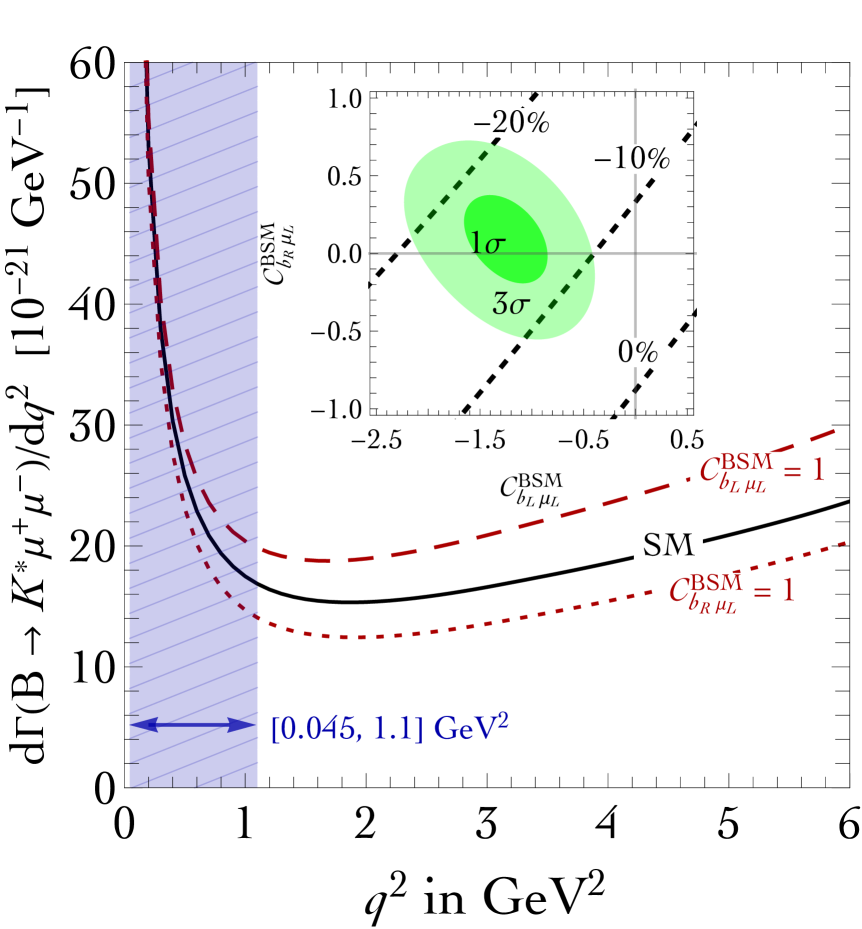
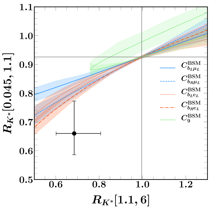
Figure 2: Left: RKsubscript𝑅superscript𝐾R_{K^{*}} as function of q2superscript𝑞2q^{2}, the invariant mass of the +superscriptsuperscript\ell^{+}\ell^{-} pair, for the SM and for two specific values of the new-physics coefficients. The inset shows iso-contours of deviation from RK=1superscriptsubscript𝑅𝐾1R_{K}^{*}=1 in the [0.045,1.1]GeV20.0451.1superscriptGeV2[0.045,1.1]\,{\rm GeV}^{2} bin as a function of new-physics coefficients, compared to their experimentally favoured values. Right: correlation between RKsubscript𝑅superscript𝐾R_{K^{*}} measured in the [1.1,6]GeV21.16superscriptGeV2[1.1,6]\,{\rm GeV}^{2} bin (horizontal axis) and [0.045,1.1]GeV20.0451.1superscriptGeV2[0.045,1.1]\,{\rm GeV}^{2} bin (vertical axis) of q2superscript𝑞2q^{2}: a sizeable new physics effect can be present in the low-energy bin. The numerical values of q2superscript𝑞2q^{2} are given in GeV2superscriptGeV2\,{\rm GeV}^{2}.

A closer look to RKsubscript𝑅superscript𝐾R_{K^{*}} reveals additional observable consequences related to the presence of BSM corrections. RKsubscript𝑅superscript𝐾R_{K^{*}}, in a given range of q2superscript𝑞2q^{2}, is defined in analogy with eq. (9):

RK[qmin2,qmax2]qmin2qmax2𝑑q2𝑑Γ(BKμ+μ)/𝑑q2qmin2qmax2𝑑q2𝑑Γ(BKe+e)/𝑑q2,subscript𝑅superscript𝐾superscriptsubscript𝑞min2superscriptsubscript𝑞max2superscriptsubscriptsuperscriptsubscript𝑞min2subscriptsuperscript𝑞2maxdifferential-dsuperscript𝑞2differential-dΓ𝐵superscript𝐾superscript𝜇superscript𝜇differential-dsuperscript𝑞2superscriptsubscriptsuperscriptsubscript𝑞min2subscriptsuperscript𝑞2maxdifferential-dsuperscript𝑞2differential-dΓ𝐵superscript𝐾superscript𝑒superscript𝑒differential-dsuperscript𝑞2R_{K^{*}}[q_{\rm min}^{2},q_{\rm max}^{2}]\equiv\frac{\int_{q_{\rm min}^{2}}^{q^{2}_{\rm max}}dq^{2}\,d\Gamma(B\to K^{*}\mu^{+}\mu^{-})/dq^{2}}{\int_{q_{\rm min}^{2}}^{q^{2}_{\rm max}}dq^{2}\,d\Gamma(B\to K^{*}e^{+}e^{-})/dq^{2}}~{}, (18)

where the differential decay width dΓ(BKμ+μ)/dq2𝑑Γ𝐵superscript𝐾superscript𝜇superscript𝜇𝑑superscript𝑞2d\Gamma(B\to K^{*}\mu^{+}\mu^{-})/dq^{2} actually describes the four-body process BK(Kπ)μ+μB\to K^{*}(\to K\pi)\mu^{+}\mu^{-}, and takes the compact form

dΓ(BKμ+μ)dq2=34(21s+2c)14(22s+2c).𝑑Γ𝐵superscript𝐾superscript𝜇superscript𝜇𝑑superscript𝑞2342superscriptsubscript1𝑠superscriptsubscript2𝑐142superscriptsubscript2𝑠superscriptsubscript2𝑐\frac{d\Gamma\left(B\to K^{*}\mu^{+}\mu^{-}\right)}{dq^{2}}=\frac{3}{4}\left(2\mathcal{I}_{1}^{s}+\mathcal{I}_{2}^{c}\right)-\frac{1}{4}\left(2\mathcal{I}_{2}^{s}+\mathcal{I}_{2}^{c}\right)~{}. (19)

The angular coefficients i=1,2a=s,csuperscriptsubscript𝑖12𝑎𝑠𝑐\mathcal{I}_{i=1,2}^{a=s,c} in eq. (19) can be written in terms of the so-called transversity amplitudes describing the decay BKV𝐵superscript𝐾superscript𝑉B\to K^{*}V^{*} with the B𝐵B meson decaying to an on-shell Ksuperscript𝐾K^{*} and a virtual photon or Z𝑍Z boson which later decays into a lepton-antilepton pair. We refer to ref. [29] for a comprehensive description of the computation. In the left panel of figure 2 we show the differential distribution dΓ(BKμ+μ)/dq2𝑑Γ𝐵superscript𝐾superscript𝜇superscript𝜇𝑑superscript𝑞2d\Gamma(B\to K^{*}\mu^{+}\mu^{-})/dq^{2} as a function of the dilepton invariant mass q2superscript𝑞2q^{2}. The solid black line represents the SM prediction, and we show in dashed (dotted) red the impact of BSM corrections due to the presence of non-zero CbLμLBSMsubscriptsuperscript𝐶BSMsubscript𝑏𝐿subscript𝜇𝐿C^{\rm BSM}_{b_{L}\mu_{L}} (CbRμLBSMsubscriptsuperscript𝐶BSMsubscript𝑏𝑅subscript𝜇𝐿C^{\rm BSM}_{b_{R}\mu_{L}}) taken at the benchmark value of 111.

We now focus on the low invariant-mass range q2=[0.045,1.1]superscript𝑞20.0451.1q^{2}=[0.045,1.1] GeV2, shaded in blue with diagonal mesh in the left panel of fig 2. In this bin, the differential rate is dominated by the SM photon contribution. It is instructive to give more quantitative comments. In the inset plot in the left panel of fig 2, we show in the plane (CbLμLBSM,CbRμLBSM)subscriptsuperscript𝐶BSMsubscript𝑏𝐿subscript𝜇𝐿subscriptsuperscript𝐶BSMsubscript𝑏𝑅subscript𝜇𝐿(C^{\rm BSM}_{b_{L}\mu_{L}},C^{\rm BSM}_{b_{R}\mu_{L}}) the relative deviation in RK[0.045,1.1]subscript𝑅superscript𝐾0.0451.1R_{K^{*}}[0.045,1.1] compared to its SM value RKSM0.9subscriptsuperscript𝑅SMsuperscript𝐾0.9R^{\rm SM}_{K^{*}}\approx 0.9, and we superimpose the 1- and 3-σ𝜎\sigma confidence contours allowed by the fit of experimental data (without including RKsubscript𝑅superscript𝐾R_{K^{*}}). This comparison shows that a 10%percent1010\% reduction of RKsubscript𝑅superscript𝐾R_{K^{*}} in the mass-invariant bin q2=[0.045,1.1]superscript𝑞20.0451.1q^{2}=[0.045,1.1] GeV2 is expected from the experimental data. The SM prediction, RKSM[0.045,1.1]0.9subscriptsuperscript𝑅SMsuperscript𝐾0.0451.10.9R^{\rm SM}_{K^{*}}[0.045,1.1]\approx 0.9, departs from one because of QED effects which distinguish between mμsubscript𝑚𝜇m_{\mu} and mesubscript𝑚𝑒m_{e}. The observed central value RKSM[0.045,1.1]=0.66subscriptsuperscript𝑅SMsuperscript𝐾0.0451.10.66R^{\rm SM}_{K^{*}}[0.045,1.1]=0.66 can be again explained with possible effects of new physics. The natural suspect is a new physics contribution to the dipole operator, but it can be shown that this cannot be very large because of bounds coming from the inclusive process BXsγ𝐵subscript𝑋𝑠𝛾B\to X_{s}\gamma, see for example ref. [30]. We can instead correlate the effect in RKSM[0.045,1.1]subscriptsuperscript𝑅SMsuperscript𝐾0.0451.1R^{\rm SM}_{K^{*}}[0.045,1.1] with RKSM[1.1,6]subscriptsuperscript𝑅SMsuperscript𝐾1.16R^{\rm SM}_{K^{*}}[1.1,6]. The results are shown in the right panel of figure 2. Here we learn that the new physics hypotheses predict values larger than the one observed in the data. However, since the experimental error is quite large, precise measurements are needed to settle this issue.

In conclusion, the picture emerging from a simple inspection of the relevant formulas for RKsubscript𝑅𝐾R_{K} and RKsubscript𝑅superscript𝐾R_{K^{*}} is very neat, and can be summarized as follows:

  • \circ

    New physics in the muon sector can easily explain the observed deficits in RKsubscript𝑅𝐾R_{K},RKsubscript𝑅superscript𝐾R_{K^{*}}, and we expect a preference for negative values of the operator involving a left-handed current, CbLμLBSMsubscriptsuperscript𝐶BSMsubscript𝑏𝐿subscript𝜇𝐿C^{\rm BSM}_{b_{L}\mu_{L}}. Sizeable deviations of RKsubscript𝑅superscript𝐾R_{K^{*}} from RKsubscript𝑅𝐾R_{K} signal non-zero values for CbRμLBSMsubscriptsuperscript𝐶BSMsubscript𝑏𝑅subscript𝜇𝐿C^{\rm BSM}_{b_{R}\mu_{L}}.

  • \circ

    New physics in the electron sector represents a valid alternative, and positive values of CbLeLBSMsubscriptsuperscript𝐶BSMsubscript𝑏𝐿subscript𝑒𝐿C^{\rm BSM}_{b_{L}e_{L}} are favoured. Sizeable deviations of RKsubscript𝑅superscript𝐾R_{K^{*}} from RKsubscript𝑅𝐾R_{K} signal non-zero values for CbReLBSMsubscriptsuperscript𝐶BSMsubscript𝑏𝑅subscript𝑒𝐿C^{\rm BSM}_{b_{R}e_{L}}. However invoking NP only the electronic channels does not allow to explain other anomalies in the muon sector such as the angular observables.

  • \circ

    There exists an interesting correlation between RKsubscript𝑅superscript𝐾R_{K^{*}} in the q2superscript𝑞2q^{2}-bin [1.1,6]1.16[1.1,6] GeV2 and [0.045,1.1]0.0451.1[0.045,1.1] GeV2. At present, all the new physics hypothesis invoked tend to predicts larger value of RKsubscript𝑅𝐾R_{K*} in the low bin than the one preferred by the data.

In section 3 we shall corroborate this qualitative picture with quantitative fits.

2.3 Bsμ+μsubscript𝐵𝑠superscript𝜇superscript𝜇B_{s}\to\mu^{+}\mu^{-}

The rate is predicted as

 BR(Bsμ+μ)BR(Bsμ+μ)SM=|CbLRμLRCbLRμLRSM|2 , BR(Bsμ+μ)BR(Bsμ+μ)SM=|CbLRμLRCbLRμLRSM|2 \fcolorbox{gray}{Gray}{~$\displaystyle\frac{\textrm{BR}(B_s \to\mu^+ \mu^-) }{\textrm{BR}(B_s \to\mu^+ \mu^-) _{\rm SM}} = \bigg|\frac{C_{b_{L-R}\mu_{L-R}}}{C^{\rm SM}_{b_{L-R}\mu_{L-R}}}\bigg|^2$~}\ , (20)

where BR(Bsμ+μ)SM=(3.65±0.23)×109BRsubscriptsubscript𝐵𝑠superscript𝜇superscript𝜇SMplus-or-minus3.650.23superscript109\textrm{BR}(B_{s}\to\mu^{+}\mu^{-})_{\textrm{SM}}=(3.65\pm 0.23)\times 10^{-9} and BR(Bsμ+μ)exp=(3.0±0.6)×109BRsubscriptsubscript𝐵𝑠superscript𝜇superscript𝜇expplus-or-minus3.00.6superscript109\textrm{BR}(B_{s}\to\mu^{+}\mu^{-})_{\textrm{exp}}=(3.0\pm 0.6)\times 10^{-9} [31]. This BR can also be affected by extra scalar operators (b¯PXs)(μ¯PYμ)¯𝑏subscript𝑃𝑋𝑠¯𝜇subscript𝑃𝑌𝜇(\bar{b}P_{X}s)(\bar{\mu}P_{Y}\mu), so that it is sometimes omitted from global BSM fits.

3 Fits

We divide the experimental data in two sets: ‘clean’ and ‘hadronic sensitive’:

  • i)

    The ‘clean’ set includes the observables discussed in the previous section: RKsubscript𝑅𝐾R_{K}, RKsubscript𝑅superscript𝐾R_{K^{*}}, to which one can add BR(Bsμ+μ)BRsubscript𝐵𝑠superscript𝜇superscript𝜇\hbox{BR}(B_{s}\to\mu^{+}\mu^{-}) given that it only provides constraints.333When using the Flavio [32] code, for consistency we include the observable BR(B0μ+μ)BRsubscript𝐵0superscript𝜇superscript𝜇\hbox{BR}(B_{0}\to\mu^{+}\mu^{-}), whose experimental error is correlated with the one on BR(Bsμ+μ)BRsubscript𝐵𝑠superscript𝜇superscript𝜇\hbox{BR}(B_{s}\to\mu^{+}\mu^{-}). The ‘cleanness’ of these observables refers to the SM prediction, in the presence of New Physics larger theoretical uncertainties are expected. We didn’t include the Q4subscript𝑄4Q_{4} and Q5subscript𝑄5Q_{5} observables measured recently by the Belle collaboration [33].

  • ii)

    The ‘hadronic sensitive’ set includes about 100 observables (summarized in the Appendix A). This list includes the branching ratios of semi-leptonic B𝐵B-meson decays as well as physical quantities extracted by the angular analysis of the decay products of the B𝐵B-mesons. Concerning the hadronic sensitivity of the angular observables, the authors of [7] argue that the optimised variables Pisubscript𝑃𝑖P_{i} have reduced theoretical uncertainties.

The rationale is to first limit the analysis to the ‘clean’ set of observables. In this way one can draw solid conclusions without relying on large and partially uncontrolled effects. This approach is aligned with the spirit of this paper, and can be extremely powerful, as already shown in section 2.2. Furthermore, extracting from this reliable theoretical environment a BSM perspective could be of primary importance to set the stage for more complex analyses. In a second and third step we will estimate the effect of the ‘hadronic sensitive’ observables and combine all observables in a global fit.

3.1 Fit to the ‘clean’ observables only

The formulæ summarized in the previous section allow us to fit the clean observables. We wrote a dedicated Flavour Anomaly Rate Tool code (Fart). For simplicity, in our χ2superscript𝜒2\chi^{2} fits we combine in quadrature the experimental errors on the two RKsubscript𝑅superscript𝐾R_{K^{*}} bins, using the higher error band when they are asymmetric. We checked that our results do not change appreciably if a more precise treatment is used.

Let us start discussing the simplest case, in which we consider one-parameter fits to each NP operator in turn. Apart from its simplicity, this hypothesis is motivated from a theoretical viewpoint, as it captures most of the relevant features of concrete models, as we shall discuss in detail in section 4. We show the corresponding results — best-fit point, 1-σ𝜎\sigma error, and Δχ2χSM2χbest2Δsuperscript𝜒2subscriptsuperscript𝜒2SMsubscriptsuperscript𝜒2best\sqrt{\Delta\chi^{2}}\equiv\sqrt{\chi^{2}_{\rm SM}-\chi^{2}_{\rm best}} — in the ‘clean’ column in table 1. In the upper part of the table we show the cases in which we allow new physics in the muon sector. It is evident that the results of the fit match the discussion of section 2.2: the left-handed coefficient CbLμLBSMsubscriptsuperscript𝐶BSMsubscript𝑏𝐿subscript𝜇𝐿C^{\rm BSM}_{b_{L}\mu_{L}} is favoured by the measured anomalies in RKsubscript𝑅𝐾R_{K} and RKsubscript𝑅superscript𝐾R_{K^{*}}, with a significance of about 4σ𝜎\sigma. We can similarly discuss the hypothesis in which we allow for new physics in the electron sector, shown in the lower part of table 1. Three cases — CbLeLBSMsubscriptsuperscript𝐶BSMsubscript𝑏𝐿subscript𝑒𝐿C^{\rm BSM}_{b_{L}e_{L}}, CbLeRBSMsubscriptsuperscript𝐶BSMsubscript𝑏𝐿subscript𝑒𝑅C^{\rm BSM}_{b_{L}e_{R}} and CbReRBSMsubscriptsuperscript𝐶BSMsubscript𝑏𝑅subscript𝑒𝑅C^{\rm BSM}_{b_{R}e_{R}} — are equally favoured by the fit. However, only the operator 𝒪bLeLsubscript𝒪subscript𝑏𝐿subscript𝑒𝐿\mathcal{O}_{b_{L}e_{L}} involving left-handed quarks and electrons can explain the observed anomalies with an order one Wilson coefficient since it dominates the new-physics corrections to both RKsubscript𝑅𝐾R_{K} and RKsubscript𝑅superscript𝐾R_{K^{*}}, see Eqs (14,17). As before, we find a statistical preference with respect to the SM case at the level of about 4-σ𝜎\sigma. To simplify the comparison with the existing literature, we show in table 2 the results of 111-parameter fits in the muon sector, this time in the vector-axial basis.

In conclusion, the piece of information that we learn from this simple fit is quite sharp: by restricting the analysis to the selected subset of ‘clean’ observables RKsubscript𝑅𝐾R_{K}, RKsubscript𝑅superscript𝐾R_{K^{*}} and BR(Bsμ+μ)BRsubscript𝐵𝑠superscript𝜇superscript𝜇{\rm BR}(B_{s}\to\mu^{+}\mu^{-}), not much affected by large theoretical uncertainties, we find a preference for the presence of new physics in the observed experimental anomalies in B𝐵B decays. In particular, the analysis selects the existence of a new neutral current that couples left-handed b𝑏b, s𝑠s quarks and left-handed muons/electrons as the preferred option.

Effective four-fermions operators that couple left- or right-handed b𝑏b, s𝑠s with right-handed electrons are also equally preferred at this level of the analysis, but they require larger numerical values of their Wilson coefficients.

New physics in the muon sector
Wilson Best-fit 1-σ𝜎\sigma range χSM2χbest2subscriptsuperscript𝜒2SMsubscriptsuperscript𝜒2best\sqrt{\chi^{2}_{\rm SM}-\chi^{2}_{\rm best}}
coeff. ‘clean’ ‘HS’ all ‘clean’ ‘HS’ all ‘clean’ ‘HS’ all
CbLμLBSMsuperscriptsubscript𝐶subscript𝑏𝐿subscript𝜇𝐿BSMC_{b_{L}\mu_{L}}^{\rm BSM} 1.271.27-1.27 1.331.33-1.33 1.301.30-1.30 0.940.94-0.94 1.011.01-1.01 1.071.07-1.07 4.14.14.1 4.64.64.6 6.26.26.2
1.621.62-1.62 1.681.68-1.68 1.551.55-1.55
CbLμRBSMsuperscriptsubscript𝐶subscript𝑏𝐿subscript𝜇𝑅BSMC_{b_{L}\mu_{R}}^{\rm BSM} 0.640.640.64 0.730.73-0.73 0.300.30-0.30 1.171.171.17 0.400.40-0.40 0.020.020.02 1.21.21.2 2.12.12.1 0.90.90.9
0.110.110.11 1.031.03-1.03 0.590.59-0.59
CbRμLBSMsuperscriptsubscript𝐶subscript𝑏𝑅subscript𝜇𝐿BSMC_{b_{R}\mu_{L}}^{\rm BSM} 0.050.050.05 0.200.20-0.20 0.140.14-0.14 0.330.330.33 0.040.04-0.04 0.000.000.00 0.20.20.2 1.31.31.3 1.01.01.0
0.230.23-0.23 0.290.29-0.29 0.250.25-0.25
CbRμRBSMsuperscriptsubscript𝐶subscript𝑏𝑅subscript𝜇𝑅BSMC_{b_{R}\mu_{R}}^{\rm BSM} 0.440.44-0.44 0.410.410.41 0.270.270.27 0.080.080.08 0.610.610.61 0.480.480.48 0.80.80.8 1.71.71.7 1.21.21.2
0.970.97-0.97 0.180.180.18 0.040.040.04
New physics in the electron sector
Wilson Best-fit 1-σ𝜎\sigma range χSM2χbest2subscriptsuperscript𝜒2SMsubscriptsuperscript𝜒2best\sqrt{\chi^{2}_{\rm SM}-\chi^{2}_{\rm best}}
coeff. ‘clean’ ‘HS’ all ‘clean’ ‘HS’ all ‘clean’ ‘HS’ all
CbLeLBSMsuperscriptsubscript𝐶subscript𝑏𝐿subscript𝑒𝐿BSMC_{b_{L}e_{L}}^{\rm BSM} 1.721.721.72 0.150.150.15 0.990.990.99 2.312.312.31 0.690.690.69 1.301.301.30 4.14.14.1 0.30.30.3 3.53.53.5
1.211.211.21 0.390.39-0.39 0.700.700.70
CbLeRBSMsuperscriptsubscript𝐶subscript𝑏𝐿subscript𝑒𝑅BSMC_{b_{L}e_{R}}^{\rm BSM} 5.155.15-5.15 1.701.70-1.70 3.463.46-3.46 4.234.23-4.23 0.330.330.33 2.812.81-2.81 4.34.34.3 0.90.90.9 3.63.63.6
6.106.10-6.10 2.832.83-2.83 4.054.05-4.05
CbReLBSMsuperscriptsubscript𝐶subscript𝑏𝑅subscript𝑒𝐿BSMC_{b_{R}e_{L}}^{\rm BSM} 0.0850.0850.085 0.510.51-0.51 0.020.020.02 0.390.390.39 0.290.290.29 0.300.300.30 0.30.30.3 0.70.70.7 0.10.10.1
0.210.21-0.21 1.551.55-1.55 0.250.25-0.25
CbReRBSMsuperscriptsubscript𝐶subscript𝑏𝑅subscript𝑒𝑅BSMC_{b_{R}e_{R}}^{\rm BSM} 5.605.60-5.60 2.102.102.10 3.633.63-3.63 4.664.66-4.66 3.523.523.52 2.652.65-2.65 4.24.24.2 0.50.50.5 2.52.52.5
6.566.56-6.56 2.702.70-2.70 4.434.43-4.43
Table 1: Best fits assuming a single chiral operator at a time, and fitting only the ‘clean’ RKsubscript𝑅𝐾R_{K}, RKsubscript𝑅superscript𝐾R_{K^{*}}, and BR(Bsμ+μ)BRsubscript𝐵𝑠superscript𝜇superscript𝜇{\rm BR}(B_{s}\to\mu^{+}\mu^{-}), or only the ‘Hadronic Sensitive’ observables (denoted by ‘HS’ in the table) as discussed in the text, or combining them in a global fit. The full list of observable can be find in appendix A.

Needless to say, this conclusion, although already very significant, must be supported by the result of a more complete analysis that accounts for all the other observables related to B𝐵B decays, and not included in the ‘clean’ set used in this section. We shall return to this point in section 3.2.

New physics in the muon sector (Vector Axial basis)
Wilson Best-fit 1-σ𝜎\sigma range χSM2χbest2subscriptsuperscript𝜒2SMsubscriptsuperscript𝜒2best\sqrt{\chi^{2}_{\rm SM}-\chi^{2}_{\rm best}}
coeff. ‘clean’ ‘HS’ all ‘clean’ ‘HS’ all ‘clean’ ‘HS’ all
C9,μBSMsuperscriptsubscript𝐶9𝜇BSMC_{9,\,\mu}^{\rm BSM} 1.511.51-1.51 1.151.15-1.15 1.191.19-1.19 1.051.05-1.05 0.980.98-0.98 1.041.04-1.04 3.93.93.9 5.55.55.5 6.76.76.7
2.082.08-2.08 1.311.31-1.31 1.351.35-1.35
C10,μBSMsuperscriptsubscript𝐶10𝜇BSMC_{10,\,\mu}^{\rm BSM} 0.970.970.97 0.480.480.48 0.660.660.66 1.281.281.28 0.690.690.69 0.830.830.83 3.83.83.8 2.42.42.4 4.34.34.3
0.690.690.69 0.280.280.28 0.500.500.50
C9,μBSMsuperscriptsubscript𝐶9𝜇BSMC_{9,\,\mu}^{\prime{\rm BSM}} 0.080.08-0.08 0.240.24-0.24 0.220.22-0.22 0.200.200.20 0.150.15-0.15 0.140.14-0.14 0.30.30.3 1.71.71.7 1.61.61.6
0.370.37-0.37 0.360.36-0.36 0.330.33-0.33
C10,μBSMsuperscriptsubscript𝐶10𝜇BSMC_{10,\,\mu}^{\prime{\rm BSM}} 0.110.11-0.11 0.100.100.10 0.070.070.07 0.110.110.11 0.190.190.19 0.150.150.15 0.50.50.5 1.21.21.2 0.90.90.9
0.340.34-0.34 0.010.010.01 0.010.01-0.01
Table 2: Same as table 1, but in the vector-axial basis.

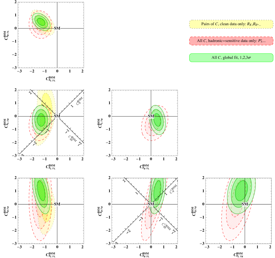
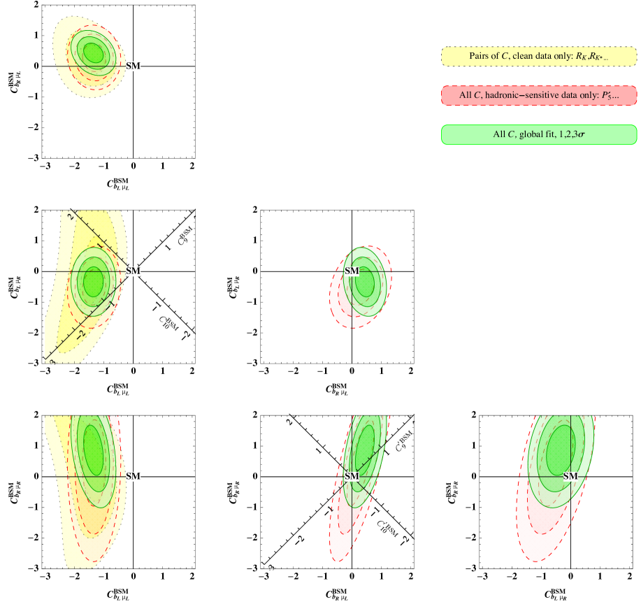
Before moving to the fit with the ‘hadronic sensitive’ observables, we perform several two-parameter fits using only ‘clean’ observables. We show our results in figure 3. Allowing for new physics in muons only, the combined best-fit regions are shown as yellow contours. Since there are few ‘clean’ observables, we turn on only two new-physics coefficients in each plot, as indicated on the axes. We also show, as rotated axes, the usual C9subscript𝐶9C_{9} and C10subscript𝐶10C_{10} coefficients. We see that the key implications mentioned in section 2.2 are confirmed by this fit, although here wider regions in parameter space are allowed. In the upper plot of figure  3 we show the results for new physics in the operators involving left-handed muons, CbLμLsubscript𝐶subscript𝑏𝐿subscript𝜇𝐿C_{b_{L}\mu_{L}} and CbRμRsubscript𝐶subscript𝑏𝑅subscript𝜇𝑅C_{b_{R}\mu_{R}}: both coefficients are fixed by the ‘clean’ data. Operators involving right-handed muons, on the other hand, do not lead to good fits. A good fit is obtained by turning on only CbLμLsubscript𝐶subscript𝑏𝐿subscript𝜇𝐿C_{b_{L}\mu_{L}}, although uncertainties do not yet allow to draw sharp conclusions.

We conclude this section with a comment on the size of the theoretical uncertainties in the presence of New Physics. While there is a consensus on the small error of the Standard Model predictions, in the presence of New Physics the “clean” observables have a larger theoretical error, barring the special case where new physics violate flavour universality while maintaining the same chiral structure of the SM (mostly LL𝐿𝐿LL at large enough q2superscript𝑞2q^{2}). As shown in figure 2, away from the Standard Model our errors are still of a few percent, in agreement with ref. [35, 36]. However, other groups [37] find a much larger theoretical error in the presence of New Physics, due to a more conservative treatment of the form factor uncertainties.444We thank Joaquim Matias for enlightening discussions about this point. Therefore, we warn the reader that the statistical significance quoted in our fits may be smaller with a different treatment of the error.

We didn’t take into account another important source of error: QED radiative corrections, calculated in ref. [3]. These are of the same order or larger than the hadronic uncertainties on RKsubscript𝑅𝐾R_{K}, RKsubscript𝑅𝐾R_{K*} in the Standard Model as predicted by Flavio. We did the exercise of inflating our hadronic error by a factor of 3, finding indeed a larger error away from the Standard Model, but still of the same order of the QED corrections.
Refer to caption
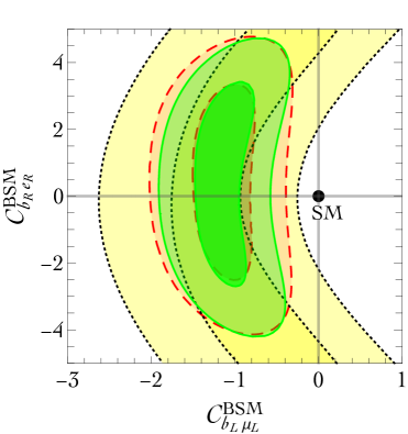
Figure 3: Fit to the new-physics contribution to the coefficients of the 4 muon operators (b¯γμPXs)(μ¯γμPYμ)¯𝑏subscript𝛾𝜇subscript𝑃𝑋𝑠¯𝜇subscript𝛾𝜇subscript𝑃𝑌𝜇(\bar{b}\gamma_{\mu}P_{X}s)(\bar{\mu}\gamma_{\mu}P_{Y}\mu), showing the 1,2,3σ123𝜎1,2,3\sigma contours. The yellow regions with dotted contours show the best fit to the ‘clean’ observables only; due to the scarcity of data, in each plot we turn on only the two coefficients indicated on its axes. The red regions with dashed contours show the best global fit to the ‘hadronic sensitive’ observables only, according to one estimate of their theoretical uncertainties; in this fit, we turn on all 4 muon operators at the same time and, in each plot, we marginalise over the coefficients not shown in the plot. The green regions show the global fit, again turning on all 4 muon operators at the same time. In figure 5 we turn on the extra 4 electron operators too.
Refer to caption      Refer to caption
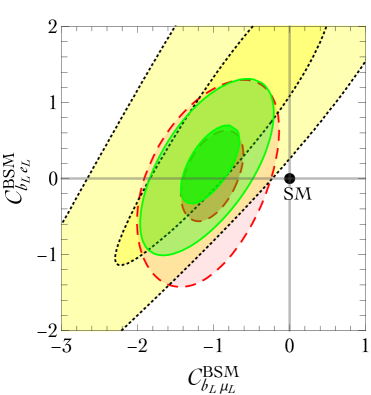
Figure 4: Fits allowing one operator involving muons (horizontal axis) and one involving electrons (vertical axis): left-handed in the left panel, and right-handed in the right panel. Regions and contours have the same meaning as in fig. 3: ‘clean’ data can be fitted by an anomaly in muons or electrons; ‘hadronic sensitive’ data favour an anomaly in muons.

3.2 Fit to the ‘hadronic sensitive’ observables

In order to perform a global fit using the ‘hadronic sensitive’ observables we use the public code Flavio [32].

Theoretical uncertainties are dominant, and it is difficult to quantify them. We first take theoretical uncertainties into account using the ‘FastFit’ method in the Flavio code with the addition of all the included nuisance parameters. With this choice, the SM is disfavoured at about 5σ5𝜎5\sigma level.

Given that most ‘hadronic sensitive’ observables involve muons (detailed measurements are much more difficult with electrons), we present a simple χ2superscript𝜒2\chi^{2} of the 4 Wilson coefficients involving muons. This is a simple useful summary of the full analysis. In this approximation, the ‘hadronic sensitive’ observables determine the 4 muon Wilson coefficients as555In general, within the Gaussian approximation, the mean values μisubscript𝜇𝑖\mu_{i}, the errors σisubscript𝜎𝑖\sigma_{i} and the correlation matrix ρijsubscript𝜌𝑖𝑗\rho_{ij} determine the χ2superscript𝜒2\chi^{2} as χ2=i,j(Ciμi)(σ2)ij1(Cjμj)superscript𝜒2subscript𝑖𝑗subscript𝐶𝑖subscript𝜇𝑖subscriptsuperscriptsuperscript𝜎21𝑖𝑗subscript𝐶𝑗subscript𝜇𝑗\chi^{2}=\sum_{i,j}(C_{i}-\mu_{i})(\sigma^{2})^{-1}_{ij}(C_{j}-\mu_{j}), where (σ2)ij=σiρijσjsubscriptsuperscript𝜎2𝑖𝑗subscript𝜎𝑖subscript𝜌𝑖𝑗subscript𝜎𝑗(\sigma^{2})_{ij}=\sigma_{i}\rho_{ij}\sigma_{j}\ .

CbLμLBSM=1.33±0.26CbRμLBSM=+0.29±0.31CbLμRBSM=0.51±0.39CbRμRBSM=+0.45±0.93withρ=(10.070.130.030.0710.250.740.130.2510.500.030.740.501).superscriptsubscript𝐶subscript𝑏𝐿subscript𝜇𝐿BSMplus-or-minus1.330.26superscriptsubscript𝐶subscript𝑏𝑅subscript𝜇𝐿BSMplus-or-minus0.290.31superscriptsubscript𝐶subscript𝑏𝐿subscript𝜇𝑅BSMplus-or-minus0.510.39superscriptsubscript𝐶subscript𝑏𝑅subscript𝜇𝑅BSMplus-or-minus0.450.93with𝜌10.070.130.030.0710.250.740.130.2510.500.030.740.501\begin{array}[]{rcl}C_{b_{L}\mu_{L}}^{\text{BSM}}&=&-1.33\pm 0.26\\ C_{b_{R}\mu_{L}}^{\text{BSM}}&=&+0.29\pm 0.31\\ C_{b_{L}\mu_{R}}^{\text{BSM}}&=&-0.51\pm 0.39\\ C_{b_{R}\mu_{R}}^{\text{BSM}}&=&+0.45\pm 0.93\\ \end{array}\qquad\hbox{with}\qquad\rho=\left(\begin{array}[]{cccc}1&-0.07&0.13&0.03\\ -0.07&1&0.25&0.74\\ 0.13&0.25&1&0.50\\ 0.03&0.74&0.50&1\\ \end{array}\right). (21)

The uncertainties can be rescaled by factors of 𝒪(1)𝒪1{\cal O}(1), if one believes that theoretical uncertainties should be larger or smaller than those adopted here.

The global fit of ‘hadronic sensitive’ observables to new physics in the 4 muon coefficients is also shown as red regions in figure 3. The important message is apparent both from the figure and from eq. (21): ‘hadronic sensitive’ observables favour a deviation from the SM in the same direction as the ‘clean’ observables, i.e. a negative contribution CbLμLBSM1similar-tosubscriptsuperscript𝐶BSMsubscript𝑏𝐿subscript𝜇𝐿1C^{\rm BSM}_{b_{L}\mu_{L}}\sim-1 to the Wilson coefficient involving left-handed quarks and muons. ‘Clean’ observables and ‘hadronic sensitive’ observables — whatever their uncertainty is — look consistent and favour independently the same pattern of deviations from the SM.

3.3 Global fit

We are now ready to combine ‘clean’ and ‘hadronic sensitive’ observables in a global fit, using both the Flavio and Fart codes. The result is shown as green regions in figure 3, assuming that new physics affects muons only. The global fit favours a deviation in the SM in CbLμLBSMsubscriptsuperscript𝐶BSMsubscript𝑏𝐿subscript𝜇𝐿C^{\rm BSM}_{b_{L}\mu_{L}}, and provides bounds on the other new-physics coefficients. Using the Gaussian approximation for the likelihood of the muon coefficients, the global fit is summarized as

CbLμLBSM=1.35±0.22CbRμLBSM=+0.44±0.21CbLμRBSM=0.33±0.33CbRμRBSM=+0.86±0.54withρ=(10.260.020.330.2610.170.470.020.1710.250.330.470.251).superscriptsubscript𝐶subscript𝑏𝐿subscript𝜇𝐿BSMplus-or-minus1.350.22superscriptsubscript𝐶subscript𝑏𝑅subscript𝜇𝐿BSMplus-or-minus0.440.21superscriptsubscript𝐶subscript𝑏𝐿subscript𝜇𝑅BSMplus-or-minus0.330.33superscriptsubscript𝐶subscript𝑏𝑅subscript𝜇𝑅BSMplus-or-minus0.860.54with𝜌10.260.020.330.2610.170.470.020.1710.250.330.470.251\begin{array}[]{rcl}C_{b_{L}\mu_{L}}^{\text{BSM}}&=&-1.35\pm 0.22\\ C_{b_{R}\mu_{L}}^{\text{BSM}}&=&+0.44\pm 0.21\\ C_{b_{L}\mu_{R}}^{\text{BSM}}&=&-0.33\pm 0.33\\ C_{b_{R}\mu_{R}}^{\text{BSM}}&=&+0.86\pm 0.54\\ \end{array}\qquad\hbox{with}\qquad\rho=\left(\begin{array}[]{cccc}1&-0.26&0.02&-0.33\\ -0.26&1&-0.17&0.47\\ 0.02&-0.17&1&0.25\\ -0.33&0.47&0.25&1\\ \end{array}\right). (22)

An anomaly in muons is strongly preferred to an anomaly in electrons, if we adopt the default estimate of the theoretical uncertainties by FLAVIO. This is for example shown in fig. 4, where we allow for a single operator involving muons and a single operator involving electrons.

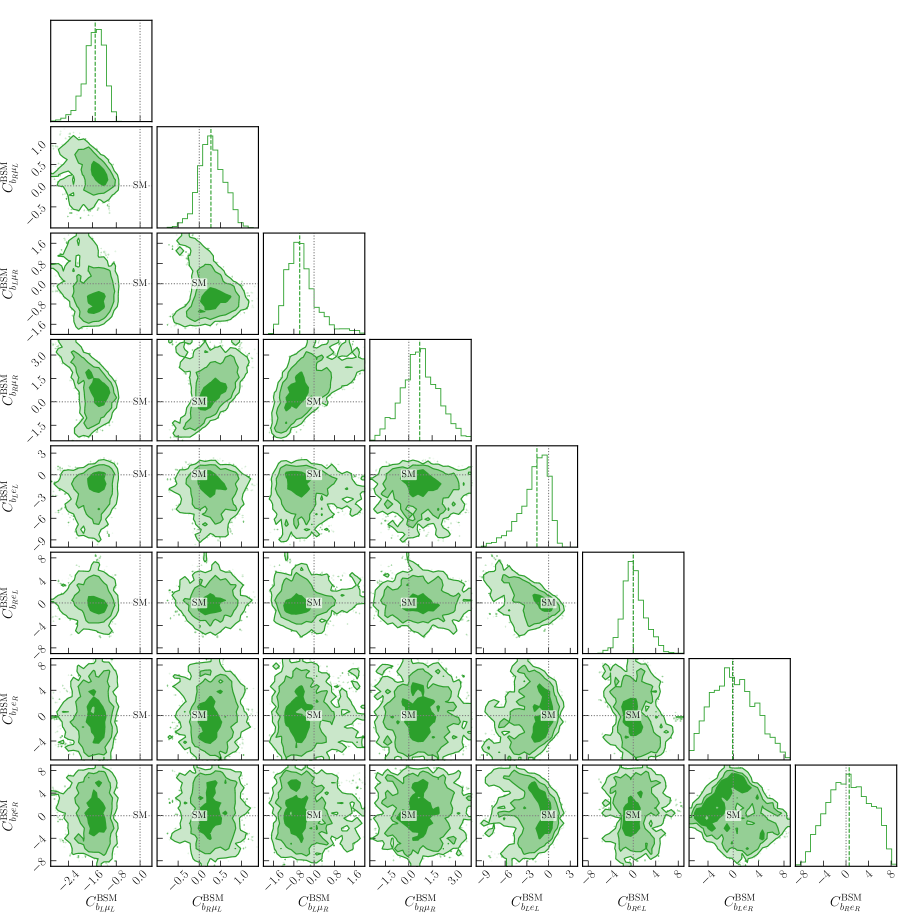
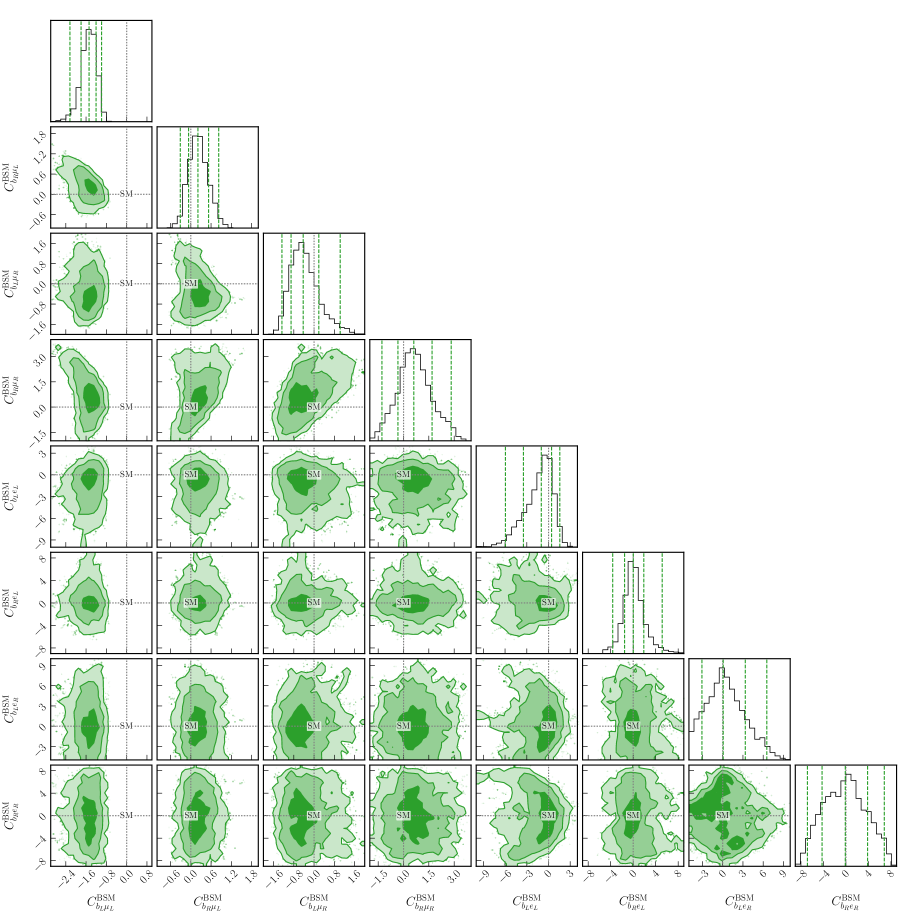
In view of this preference, and given the scarcity of data in the electron sector, we avoid presenting a global fit of new physics in electrons only. We instead perform a global combined fit for the muon and electron coefficients (which should be interpreted with caution, given that ‘hadronic sensitive’ observables are dominated by theoretical uncertainties). We find the result shown in figure 5, which confirms that — while electrons can be affected by new physics — ‘hadronic sensitive’ data favour an anomaly in muons.

The latter result has been obtained by a global Bayesian fit to the observables listed in tables 6, 7 in addition to the clean observables. We used the Flavio code to calculate the likelihood, and we sampled the posterior using the Emcee code [38], assuming for the 8 Wilson coefficients (at the scale 160GeV160GeV160\,{\rm GeV}) a flat prior between 1010-10 and 101010. In this global fit, we choose to marginalize over 252525 nuisance parameters only, to keep computational times within reasonable limits. The nuisances (form factors related to B𝐵B decays) are selected in the following way. For each observable, we define theoretical uncertainties due to changing each nuisance within its uncertainty, keeping the others fixed at their central values. Then, we choose to marginalize only over the parameters which give a theoretical uncertainty larger than the experimental error on the observable.
Refer to caption
Figure 5: Global fit to the 8 Wilson coefficients in muons and electrons, combining ‘clean’ and ‘hadronic sensitive’ data.
Refer to caption
Figure 6: Particles that can mediate RKsubscript𝑅𝐾R_{K} at tree level: a Zsuperscript𝑍Z^{\prime} or a lepto-quark, scalar or vector.

4 Theoretical interpretations

We now discuss different theoretical interpretations that can accommodate the flavour anomalies. We start with the observation that an effective (s¯γμPXb)(¯γμPY)¯𝑠subscript𝛾𝜇subscript𝑃𝑋𝑏¯subscript𝛾𝜇subscript𝑃𝑌(\bar{s}\gamma_{\mu}P_{X}b)(\bar{\ell}\gamma_{\mu}P_{Y}\ell) interaction can be mediated at tree level by two kinds of particle: a Zsuperscript𝑍Z^{\prime} or a leptoquark. Higher-order induced mechanisms are also possible. These models tend to generate related operators

cbLbL(s¯γμPLb)2+cμLνμ(μ¯γμPLμ)(ν¯μγμPLνμ),subscript𝑐subscript𝑏𝐿subscript𝑏𝐿superscript¯𝑠subscript𝛾𝜇subscript𝑃𝐿𝑏2subscript𝑐subscript𝜇𝐿subscript𝜈𝜇¯𝜇superscript𝛾𝜇subscript𝑃𝐿𝜇subscript¯𝜈𝜇subscript𝛾𝜇subscript𝑃𝐿subscript𝜈𝜇c_{b_{L}b_{L}}(\bar{s}\gamma_{\mu}P_{L}b)^{2}+c_{\mu_{L}\nu_{\mu}}(\bar{\mu}\gamma^{\mu}P_{L}\mu)(\bar{\nu}_{\mu}\gamma_{\mu}P_{L}\nu_{\mu})\ , (23)

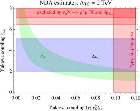
and therefore one needs to consider the associated experimental constraints. The first operator affects Bssubscript𝐵𝑠B_{s} mass mixing for which the relative measurements, together with CKM fits, imply cbLbLBSM=(0.09±0.08)/(110TeV)2subscriptsuperscript𝑐BSMsubscript𝑏𝐿subscript𝑏𝐿plus-or-minus0.090.08superscript110TeV2c^{\rm BSM}_{b_{L}b_{L}}=(-0.09\pm 0.08)/(110\,{\rm TeV})^{2} , i.e. the bound |cbLbLBSM|<1/(210TeV)2subscriptsuperscript𝑐BSMsubscript𝑏𝐿subscript𝑏𝐿1superscript210TeV2|c^{\rm BSM}_{b_{L}b_{L}}|<1/(210\,{\rm TeV})^{2} [11, 39]. The second operator is constrained by CCFR data on the neutrino trident cross section, yielding the weaker bound |cμLνμBSM|<1/(490GeV)2subscriptsuperscript𝑐BSMsubscript𝜇𝐿subscript𝜈𝜇1superscript490GeV2|c^{\rm BSM}_{\mu_{L}\nu_{\mu}}|<1/(490\,{\rm GeV})^{2} at 95% C.L. [40]. Furthermore, new physics that affects muons can contribute to the anomalous magnetic moment of the muon. Experiments found hints of a possible deviation from the Standard Model with Δaμ=(24±9)1010Δsubscript𝑎𝜇plus-or-minus249superscript1010\Delta a_{\mu}=(24\pm 9)\cdot 10^{-10} [41].

4.1 Models with an extra Zsuperscript𝑍Z^{\prime}

Models featuring extra Zsuperscript𝑍Z^{\prime} to explain the anomalies are very popular, see the partial list of references [42, 43, 44, 45, 46, 47, 48, 49, 50, 51, 52, 53, 54, 55, 56, 57, 58, 59, 60, 61]. Typically these models contain a Zsuperscript𝑍Z^{\prime} with mass MZsubscript𝑀superscript𝑍M_{Z^{\prime}} savagely coupled to

[gbs(s¯γμPLb)+h.c.]+gμL(μ¯γμPLμ).delimited-[]subscript𝑔𝑏𝑠¯𝑠subscript𝛾𝜇subscript𝑃𝐿𝑏h.c.subscript𝑔subscript𝜇𝐿¯𝜇subscript𝛾𝜇subscript𝑃𝐿𝜇[g_{bs}(\bar{s}\gamma_{\mu}P_{L}b)+\hbox{h.c.}]+g_{\mu_{L}}(\bar{\mu}\gamma_{\mu}P_{L}\mu)\ . (24)

The model can reproduce the flavour anomalies with cbLμL=gbsgμL/MZ2subscript𝑐subscript𝑏𝐿subscript𝜇𝐿subscript𝑔𝑏𝑠subscript𝑔subscript𝜇𝐿superscriptsubscript𝑀superscript𝑍2c_{b_{L}\mu_{L}}=-g_{bs}g_{\mu_{L}}/M_{Z^{\prime}}^{2} as illustrated in figure 6a. At the same time the Zsuperscript𝑍Z^{\prime} contributes to the Bssubscript𝐵𝑠{B_{s}} mass mixing with cbLbL=gbs2/2MZ2subscript𝑐subscript𝑏𝐿subscript𝑏𝐿superscriptsubscript𝑔𝑏𝑠22superscriptsubscript𝑀superscript𝑍2c_{b_{L}b_{L}}=-g_{bs}^{2}/2M_{Z^{\prime}}^{2}. The bound from ΔMBsΔsubscript𝑀subscript𝐵𝑠\Delta M_{B_{s}} can be satisfied by requiring a large enough gμLsubscript𝑔subscript𝜇𝐿g_{\mu_{L}} in order to reproduce the bs+𝑏𝑠superscriptsuperscriptb\to s\ell^{+}\ell^{-} anomalies. Left-handed leptons are unified in a SU(2)LSUsubscript2𝐿\,{\rm SU}(2)_{L} doublet L=(νL,L)𝐿subscript𝜈𝐿subscript𝐿L=(\nu_{L},\ell_{L}), such that also the neutrino operator cμLνμ=gμL2/MZ2subscript𝑐subscript𝜇𝐿subscript𝜈𝜇superscriptsubscript𝑔subscript𝜇𝐿2superscriptsubscript𝑀superscript𝑍2c_{\mu_{L}\nu_{\mu}}=-g_{\mu_{L}}^{2}/M_{Z^{\prime}}^{2} is generated. However the latter does not yield a strong constraint on gμLsubscript𝑔subscript𝜇𝐿g_{\mu_{L}}.

Another possibility is for the Zsuperscript𝑍Z^{\prime} to couple to the 3-rd generation left-handed quarks with coupling gtsubscript𝑔𝑡g_{t} and to lighter left-handed quarks with coupling gqsubscript𝑔𝑞g_{q}. The coupling gbssubscript𝑔𝑏𝑠g_{bs} arises as gbs=(gtgq)(UQd)tssubscript𝑔𝑏𝑠subscript𝑔𝑡subscript𝑔𝑞subscriptsubscript𝑈subscript𝑄𝑑𝑡𝑠g_{bs}=(g_{t}-g_{q})(U_{Q_{d}})_{ts} after performing a flavour rotation UQdsubscript𝑈subscript𝑄𝑑U_{Q_{d}} among left-handed down quarks to their mass-eigenstate basis. The matrix element (UQd)tssubscriptsubscript𝑈subscript𝑄𝑑𝑡𝑠(U_{Q_{d}})_{ts} is presumably not much larger than Vtssubscript𝑉𝑡𝑠V_{ts} and possibly equal to it, if the CKM matrix V=UQuUQd𝑉subscript𝑈subscript𝑄𝑢superscriptsubscript𝑈subscript𝑄𝑑V=U_{Q_{u}}U_{Q_{d}}^{\dagger} is dominated by the rotation among left-handed down quarks, rather than by the rotation UQusubscript𝑈subscript𝑄𝑢U_{Q_{u}} among left-handed up quarks.

Unless gq=0subscript𝑔𝑞0g_{q}=0, the parameter space of the Zsuperscript𝑍Z^{\prime} model gets severely constrained by combining perturbative bounds on gμLsubscript𝑔subscript𝜇𝐿g_{\mu_{L}}. In addition the LHC bounds on ppZμμ¯𝑝𝑝superscript𝑍𝜇¯𝜇pp\to Z^{\prime}\to\mu\bar{\mu} can be relaxed by introducing extra features, such as a Zsuperscript𝑍Z^{\prime} branching ratio into invisible DM particles [62].

A characteristic feature of Zsuperscript𝑍Z^{\prime} models is that they can mediate effective operators involving different chiralities. In fact, gauge-anomaly cancellations also induce multiple chiralities: for example a Zsuperscript𝑍Z^{\prime} coupled to LμLτsubscript𝐿𝜇subscript𝐿𝜏L_{\mu}-L_{\tau} is anomaly free [44], where the Lesubscript𝐿𝑒L_{e} contribution is avoided because LEP put strong constraints on 4-electron operators. The chiralities involved in the bs+𝑏𝑠superscriptsuperscriptb\to s\ell^{+}\ell^{-} anomalies can be determined trough more precise measurements of ‘clean’ observables such as RKsubscript𝑅𝐾R_{K} and RKsubscript𝑅superscript𝐾R_{K^{*}}.

4.2 Models with lepto-quarks

The anomalous effects in bs+𝑏𝑠superscriptsuperscriptb\to s\ell^{+}\ell^{-} transitions might be due to the exchange of a Lepto-Quark (LQ), namely a boson that couples to a lepton and a quark. Concerning lepton flavour, in general a LQ can couple to both muons and electrons. However, simultaneous sizeable couplings of a LQ to electrons and muons generates lepton flavour violation which is severely constrained by the time-honoured radiative decay μeγ𝜇𝑒𝛾\mu\to e\gamma. For this reason one typically assumes that LQs couple to either electrons or muons. (Here sizeable means an effect which has an impact on the anomalous observables). The coupling to muons allows to fit the anomalies in bsμ+μ𝑏𝑠superscript𝜇superscript𝜇b\to s\mu^{+}\mu^{-} distributions, as well as the RKsubscript𝑅𝐾R_{K} and RKsubscript𝑅superscript𝐾R_{K^{*}} μ/e𝜇𝑒\mu/e ratios.

The gauge quantum numbers of scalar LQs select a specific chirality of the SM fermions involved in the new Yukawa couplings, and thereby generate a unique characteristic operator in the effective Lagrangian in the chiral basis of eq. (5), as illustrated in figure 6b. The correspondence is given by

CoefficientLepto-QuarkYukawa couplingsCbLLS3(3¯,3,1/3)yQLS3+yQQS3+h.c.CbLRR2(3,2,7/6)yULR2+yQER2+h.c.CbRLR~2(3,2,1/6)yDLR~2+h.c.CbRRS~1(3¯,1,4/3)yDES~1+yUUS~1+h.c.CoefficientLepto-QuarkYukawa couplingsmissing-subexpressionmissing-subexpressionmissing-subexpressionsubscript𝐶subscript𝑏𝐿subscript𝐿similar-tosubscript𝑆3¯3313𝑦𝑄𝐿subscript𝑆3superscript𝑦𝑄𝑄subscriptsuperscript𝑆3h.c.subscript𝐶subscript𝑏𝐿subscript𝑅similar-tosubscript𝑅23276𝑦𝑈𝐿subscript𝑅2superscript𝑦𝑄𝐸subscriptsuperscript𝑅2h.c.subscript𝐶subscript𝑏𝑅subscript𝐿similar-tosubscript~𝑅23216𝑦𝐷𝐿subscript~𝑅2h.c.subscript𝐶subscript𝑏𝑅subscript𝑅similar-tosubscript~𝑆1¯3143𝑦𝐷𝐸subscript~𝑆1superscript𝑦𝑈𝑈subscriptsuperscript~𝑆1h.c.\begin{array}[]{ccc}\hbox{Coefficient}&\hbox{Lepto-Quark}&\hbox{Yukawa couplings}\\ \hline\cr C_{b_{L}\ell_{L}}&S_{3}\sim({\bar{3}},{3},1/3)&y\,QL\,S_{3}+y^{\prime}\,QQ\,S^{\dagger}_{3}+\hbox{h.c.}\\ C_{b_{L}\ell_{R}}&R_{2}\sim(3,{2},7/6)&y\,UL\,R_{2}+y^{\prime}\,QE\,R^{\dagger}_{2}+\hbox{h.c.}\\ C_{b_{R}\ell_{L}}&\tilde{R}_{2}\sim(3,{2},1/6)&y\,DL\,\tilde{R}_{2}+\hbox{h.c.}\\ C_{b_{R}\ell_{R}}&\tilde{S}_{1}\sim({\bar{3}},{1},4/3)&y\,DE\,\tilde{S}_{1}+y^{\prime}\,UU\,\tilde{S}^{\dagger}_{1}+\hbox{h.c.}\end{array} (25)

where \ell can be either an electron or a muon. In parentheses we report the SU(3)×SU(2)L×U(1)YSU3SUsubscript2𝐿Usubscript1𝑌\,{\rm SU}(3)\times\,{\rm SU}(2)_{L}\times{\rm U}(1)_{Y} gauge quantum numbers, and we follow the notations and conventions from ref. [63] for LQ names. Q,L𝑄𝐿Q,L (U,D,E𝑈𝐷𝐸U,D,E) denote the left-handed (right-handed) SM quarks and leptons.

Given that each LQ mediates effective operators with a given chirality, we can draw conclusions from our one parameter fits of the bs+𝑏𝑠superscriptsuperscriptb\to s\ell^{+}\ell^{-} anomalies of table 1. Assuming new physics in the muon sector, the measurement of RKsubscript𝑅superscript𝐾R_{K^{*}} selects a unique scalar lepto-quark: S3(3¯,3,1/3)similar-tosubscript𝑆3¯3313S_{3}\sim({\bar{3}},{3},1/3), which is a triplet under SU(2)LSUsubscript2𝐿\,{\rm SU}(2)_{L}. It is remarkable that this is obtained with just the information coming from ‘clean’ observables while the inclusion of the remaining observables (with our specified treatment of the errors) reinforces this hypothesis. The explanation of the anomalies in terms of S3subscript𝑆3S_{3} has been firstly proposed after the measurement of RKsubscript𝑅𝐾R_{K} in ref. [10] switching on only those couplings needed to reproduce the effect. In ref. [64] the LQ has been identified as a pseudo-Goldstone boson associated to the breaking of a global symmetry of a new strongly coupled sector [65]. In ref. [65, 64] it has also been suggested that a rationale for the size of the various flavour couplings could be dictated by the mechanism of partial compositeness [66]. Another motivated pattern of couplings has been suggested in ref. [67] using flavour symmetry. Also ref. [68] makes use of S3subscript𝑆3S_{3} as mediator of the bsμ+μ𝑏𝑠superscript𝜇superscript𝜇b\to s\mu^{+}\mu^{-} transition.

A potential issue with S3subscript𝑆3S_{3} is the danger of extra renormalizable couplings with di-quarks (denoted collectively by ysuperscript𝑦y^{\prime} in the Lagrangians above) which may induce proton decay. Baryon number conservation has to be invoked to avoid this issue. Motivated by this, in ref. [69, 70], the LQ R~2subscript~𝑅2\tilde{R}_{2} (which respects the global symmetry U(1)Bsubscript1𝐵(1)_{B} accidentally at the renormalizable level) has been considered leading to the prediction RK>1subscript𝑅superscript𝐾1R_{K^{*}}>1, which is now disfavoured by the LHCb data. The other two options S~1subscript~𝑆1\tilde{S}_{1} and R2subscript𝑅2R_{2} were already disfavoured after the measurement of RKsubscript𝑅𝐾R_{K} [10, 71].

The situation is different if LQs couple to electrons, rather than to muons, such that only the anomalies in the ‘clean’ observables can be reproduced. ‘Clean’ observables can be reproduced by all chiralities, with the only exclusion of CbRLsubscript𝐶subscript𝑏𝑅subscript𝐿C_{b_{R}\ell_{L}}, which is mediated by the R~2subscript~𝑅2\tilde{R}_{2} LQ. From the fit, we notice that the S~1subscript~𝑆1\tilde{S}_{1} and R2subscript𝑅2R_{2} LQs can only fit the anomalies by giving a large contribution to the Wilson coefficients, comparable to the SM contributions: this happens because these LQs couple to right handed electrons, with little interference with the SM. One the other hand, S3subscript𝑆3S_{3} couples to left-handed leptons, such that the sizeable interference with the SM allows to reproduce the observed anomalies with a smaller new physics component.

SpinQuantumClean observablesClean observablesAllNumbernew physics in enew physics in μobservablesS30(3¯,3,1/3)R20(3,2,7/6)R~20(3,2,1/6)S~10(3¯,1,4/3)U31(3,3,2/3)V21(3¯,2,5/6)U11(3¯,1,2/3)missing-subexpressionSpinQuantumClean observablesClean observablesAllmissing-subexpressionmissing-subexpressionNumbernew physics in 𝑒new physics in 𝜇observablesmissing-subexpressionmissing-subexpressionmissing-subexpressionmissing-subexpressionmissing-subexpressionmissing-subexpressionmissing-subexpressionmissing-subexpressionmissing-subexpressionmissing-subexpressionmissing-subexpressionmissing-subexpressionsubscript𝑆30¯3313subscript𝑅203276missing-subexpressionmissing-subexpressionsubscript~𝑅203216missing-subexpressionmissing-subexpressionmissing-subexpressionsubscript~𝑆10¯3143missing-subexpressionmissing-subexpressionmissing-subexpressionmissing-subexpressionmissing-subexpressionmissing-subexpressionmissing-subexpressionmissing-subexpressionsubscript𝑈313323subscript𝑉21¯3256missing-subexpressionmissing-subexpressionsubscript𝑈11¯3123\begin{array}[]{c|c|c|c|c|c}&\textrm{Spin}&\textrm{Quantum}&\textrm{Clean observables}&\textrm{Clean observables}&\textrm{All}\\ &&\textrm{Number}&\textrm{new physics in }e&\textrm{new physics in }\mu&\textrm{observables}\\ \hline\cr\hline\cr S_{3}&0&({\bar{3}},{3},1/3)&\checkmark&\checkmark&\checkmark\\ R_{2}&0&(3,{2},7/6)&\checkmark&&\\ \tilde{R}_{2}&0&(3,{2},1/6)&&&\\ \tilde{S}_{1}&0&({\bar{3}},{1},4/3)&\checkmark&&\\ \hline\cr U_{3}&1&(3,3,2/3)&\checkmark&\checkmark&\checkmark\\ V_{2}&1&(\overline{3},2,5/6)&\checkmark&&\\ U_{1}&1&(\overline{3},1,2/3)&\checkmark&\checkmark&\checkmark\\ \end{array}
Table 3: Which lepto-quarks can reproduce which bs+𝑏𝑠superscriptsuperscriptb\to s\ell^{+}\ell^{-} anomalies.

We briefly comment on the possible interpretation of a LQ as a supersymmetric particle in the MSSM. The only sparticle with the same gauge quantum numbers as a LQ is the left-handed squark Q~R~2similar-to~𝑄subscript~𝑅2\tilde{Q}\sim\tilde{R}_{2}. However, even if it has R𝑅R-parity violating interactions, this LQ gives the wrong correlation between RKsubscript𝑅𝐾R_{K} and RKsubscript𝑅superscript𝐾R_{K^{*}}, disfavouring the supersymmetric interpretation of the anomalies.

We move now to the discussion of the exchange of vector LQs at tree level, illustrated in figure 6c. There are 3 cases: U3(3,3,2/3)similar-tosubscript𝑈33323U_{3}\sim(3,3,2/3), V2(3¯,2,5/6)similar-tosubscript𝑉2¯3256V_{2}\sim(\overline{3},2,5/6) and U1(3¯,1,2/3)similar-tosubscript𝑈1¯3123U_{1}\sim(\overline{3},1,2/3). Their relevant interactions are:

LU3=Q¯γμL   U3μ+h.c. \\ LV2=yD¯γμLV2μ+yQ¯γμEV2μ+y′′Q¯γμUV2μ+h.c.\\U1=yQ¯γμLU1μ+y2D¯γμEU1μ+h.c.(26)subscriptLsubscriptU3=¯QsubscriptγμsubscriptsuperscriptL   Uμ3subscript+h.c. \\ LsubscriptV2=𝑦¯𝐷subscript𝛾𝜇𝐿superscriptsubscript𝑉2𝜇superscript𝑦¯𝑄subscript𝛾𝜇𝐸superscriptsubscript𝑉2𝜇superscript𝑦′′¯𝑄subscript𝛾𝜇𝑈superscriptsubscript𝑉2absent𝜇h.c.\\subscriptsubscript𝑈1𝑦¯𝑄subscript𝛾𝜇𝐿superscriptsubscript𝑈1𝜇subscript𝑦2¯𝐷subscript𝛾𝜇𝐸superscriptsubscript𝑈1𝜇h.c.26\halign to=0.0pt{\@eqnsel\hskip\@centering$\displaystyle{#}$&\global\@eqcnt\@ne\hskip 2\arraycolsep\hfil${#}$\hfil& \global\@eqcnt\tw@\hskip 2\arraycolsep$\displaystyle{#}$\hfil&\llap{#}\cr 0.0pt plus 1000.0pt$\displaystyle{\mathscr{L}_{U_{3}} &10.0pt\hfil${=&10.0pt$\displaystyle{y \, \bar{Q} \gamma_{\mu} L \, U^{\mu}_{3} +\hbox{h.c.} \\ \mathscr{L}_{V_{2}} &\hbox to0.0pt{\hss=&y\,\bar{D}\gamma_{\mu}L\,V_{2}^{\mu}+y^{\prime}\,\bar{Q}\gamma_{\mu}E\,V_{2}^{\mu}+y^{\prime\prime}\,\bar{Q}\gamma_{\mu}U\,V_{2}^{\dagger\mu}+\hbox{h.c.}\\\mathscr{L}_{U_{1}}&=&y\,\bar{Q}\gamma_{\mu}L\,U_{1}^{\mu}+y_{2}\,\bar{D}\gamma_{\mu}E\,U_{1}^{\mu}+\hbox{h.c.}&(26)\cr}}}}}

The vector LQ V2subscript𝑉2V_{2} and U1subscript𝑈1U_{1} can contribute to the anomalous observables trough multiple chiral structures. In general, if both y𝑦y and ysuperscript𝑦y^{\prime} are sizeable, dangerous scalar operators may be generated. If one of the two couplings dominates, we can again restrict to our one parameter fit, with the following correspondence: CbLLsubscript𝐶subscript𝑏𝐿subscript𝐿C_{b_{L}\ell_{L}} can be generated by U3subscript𝑈3U_{3}; CbLRsubscript𝐶subscript𝑏𝐿subscript𝑅C_{b_{L}\ell_{R}} or CbRLsubscript𝐶subscript𝑏𝑅subscript𝐿C_{b_{R}\ell_{L}} can be generated by V2subscript𝑉2V_{2}; CbLLsubscript𝐶subscript𝑏𝐿subscript𝐿C_{b_{L}\ell_{L}} or CbRRsubscript𝐶subscript𝑏𝑅subscript𝑅C_{b_{R}\ell_{R}} can be generated by U1subscript𝑈1U_{1}.

Similar phenomenological considerations to explain the B𝐵B-meson anomalies as in the case of the scalar LQ apply, we summarise the relevant options in table 3.

Models featuring vector LQs models in order to explain the flavour anomalies appeared recently in the literature [72, 73, 74, 75], typically as new composite states. The presence of these states signals that the theory in isolation is non-renormalizable, meaning that loop effects of the vectors are UV divergent, for a recent re-discussion see ref. [76]. Naive dimensional analysis shows that one-loop contributions to physics observables such ΔMBsΔsubscript𝑀subscript𝐵𝑠\Delta M_{B_{s}} might be problematic. A careful study of this topic is a model dependent issue and it requires extra information on the UV embedding of the LQ in a complete theory.
Refer to caption
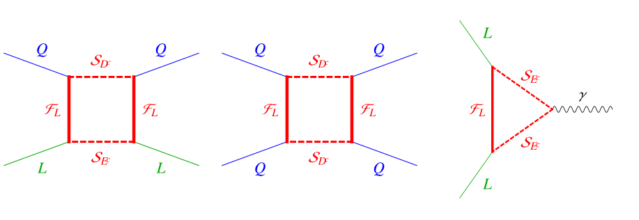
Figure 7: Feynman diagrams contributing to RKsubscript𝑅𝐾R_{K}, ΔMBsΔsubscript𝑀subscript𝐵𝑠\Delta M_{B_{s}} and the muon g2𝑔2g-2 in models with extra fermions {\cal F} and extra scalars 𝒮𝒮{\cal S}. In Fundamental Composite Higgs models these diagrams will be dressed by further new composite dynamic contributions.

4.3 Models with loop mediators

The RKsubscript𝑅𝐾R_{K} anomaly can be reproduced by one loop diagrams involving new scalars 𝒮𝒮{\cal S} and new fermions {\cal F} with Yukawa couplings to SM fermions that allow for the Feynman diagram on the left in figure 7 [77, 39] – see also ref. [78]. In this particular example, one generates an operator involving left-handed SM quarks and leptons, denoted respectively by Q𝑄Q and L𝐿L. The needed extra Yukawa coupling to the muon must be large, yL1.5similar-tosubscript𝑦𝐿1.5y_{L}\sim 1.5. This also explains why the MSSM does not allow for an explanation of the RK,RKsubscript𝑅𝐾subscript𝑅superscript𝐾{R_{K}},R_{K^{*}} anomalies: a possibile box diagram containing Winos and sleptons predicts yLg21.5similar-tosubscript𝑦𝐿subscript𝑔2much-less-than1.5y_{L}\sim g_{2}\ll 1.5, where g2subscript𝑔2g_{2} is the SU(2)LSUsubscript2𝐿\,{\rm SU}(2)_{L} gauge coupling.

In section 4.4 we will consider renomalizable models of composite dynamics featuring extra elementary scalars, where we will show that the extra particles 𝒮𝒮{\cal S} and {\cal F} can be identified with the constituents of the Higgs boson, and that their Yukawa couplings are the source of the SM Yukawa couplings, giving rise to a flavour structure similar to the SM structure. Then, the one loop Feynman diagrams of figure 7 are dressed by the underlying composite dynamic.

4.4 Fundamental composite Higgs

Models in which the Higgs is a composite state are prime candidates as potential source of new physics in the flavour sector [79, 80, 81]. Fundamental theories with a Higgs as a composite state that are also able to generate SM fermion masses appeared in ref. [82]. These theories feature both techni-scalars 𝒮𝒮{\cal S} and techni-fermions {\cal F}.666Composite theories including TC scalars attempting to give masses to the SM quarks appeared earlier in the literature [83, 84, 85, 86, 87, 88] for (walking) TC theories that didn’t feature a light Higgs. In models of fundamental composite Higgs: i) it is possible to replace the standard model Higgs and Yukawa sectors with a composite Higgs made of techni-particles; ii) the SM fermion masses are generated via a partial compositeness mechanism [66] in which the relevant composite techni-baryons emerge as bound states of a techni-fermion and a techni-scalar.

The composite theory does not address the SM naturalness issue and it is fundamental in the sense that it can be extrapolated till the Planck scale [82]. Having a fundamental theory of composite Higgs, we use it to investigate the flavour anomalies.

namespingenerationsSU(3)cSU(2)LU(1)YSU(3)TCL1/2112Y=1/23Nc1/2111Y1/2=03Ec1/2111Y1/2=13𝒮Ec0311Y1/2=13𝒮Dc0331Y+1/6=1/33missing-subexpressionmissing-subexpressionmissing-subexpressionmissing-subexpressionmissing-subexpressionmissing-subexpressionmissing-subexpressionnamespingenerationsSUsubscript3𝑐SUsubscript2𝐿Usubscript1𝑌SUsubscript3TCmissing-subexpressionmissing-subexpressionmissing-subexpressionmissing-subexpressionmissing-subexpressionmissing-subexpressionmissing-subexpressionsubscript𝐿12112𝑌123superscriptsubscript𝑁𝑐12111𝑌1203subscriptsuperscript𝐸𝑐12111𝑌1213subscript𝒮superscript𝐸𝑐0311𝑌1213subscript𝒮superscript𝐷𝑐0331𝑌16133\begin{array}[]{|ccc|cccc|}\hline\cr\hbox{name}&\hbox{spin}&\hbox{generations}&\,{\rm SU}(3)_{c}&\,{\rm SU}(2)_{L}&\,{\rm U}(1)_{Y}&\,{\rm SU}(3)_{\rm TC}\\ \hline\cr{\cal F}_{L}&1/2&1&1&2&Y=-1/2&3\\ {\cal F}_{N}^{c}&1/2&1&1&1&-Y-1/2=0&3\\ {\cal F}_{E^{c}}&1/2&1&1&1&Y-1/2=-1&3\\ {\cal S}_{E^{c}}&0&3&1&1&Y-1/2=-1&3\\ {\cal S}_{D^{c}}&0&3&3&1&Y+1/6=-1/3&3\\ \hline\cr\end{array}
Table 4: Field content of the simplest Fundamental Composite Higgs model. Extra fermions Nc,L,Ecsuperscriptsubscript𝑁𝑐subscript𝐿subscriptsuperscript𝐸𝑐{\cal F}_{N}^{c},{\cal F}_{L},{\cal F}_{E^{c}} with conjugated gauge quantum numbers such that the fermion content is vectorial are implicit. Names are appropriate assuming the value Y=1/2𝑌12Y=-1/2 for the hypercharge Y𝑌Y of Lsubscript𝐿{\cal F}_{L}; however generic values are allowed.

The gauge group and the field content of a simple model are summarised in table 4. Here the new strong group is chosen to be SU(NTC)SUsubscript𝑁TC\,{\rm SU}(N_{\rm TC}) with NTC=3subscript𝑁TC3N_{\rm TC}=3 and we list the gauge quantum numbers of the new vectorial fermions and scalars that can provide a composite Higgs with Yukawa couplings to all SM fermions L,E,Q,U,D𝐿𝐸𝑄𝑈𝐷L,E,Q,U,D. Three generations of techni-scalars are introduced in order to reproduce all SM fermion masses and mixings, while having a renormalizable theory with no Landau poles below the Planck scale. The hypercharge Y𝑌Y of the Lsubscript𝐿{\cal F}_{L} fermion is free. We assume the minimal choices Y=1/2𝑌12Y=-1/2, Y=1/2𝑌12Y=1/2 and Y=0𝑌0Y=0.

The matrices of SM Yukawa couplings ysubscript𝑦y_{\ell}, yusubscript𝑦uy_{\rm u}, ydsubscript𝑦dy_{\rm d} are obtained from the TC-Yukawa couplings

Y=yLLL𝒮Ec+yEENc𝒮Ec+(yDDNc+yUUEcc)𝒮Dc+yQQL𝒮Dc+h.c.subscript𝑌subscript𝑦𝐿𝐿subscript𝐿superscriptsubscript𝒮superscript𝐸𝑐subscript𝑦𝐸𝐸superscriptsubscript𝑁𝑐subscript𝒮superscript𝐸𝑐subscript𝑦𝐷𝐷superscriptsubscript𝑁𝑐subscript𝑦𝑈𝑈superscriptsubscriptsuperscript𝐸𝑐𝑐subscript𝒮superscript𝐷𝑐subscript𝑦𝑄𝑄subscript𝐿superscriptsubscript𝒮superscript𝐷𝑐h.c.\mathscr{L}_{Y}=y_{L}\,L{\cal F}_{L}{\cal S}_{E^{c}}^{*}+y_{E}\,E{\cal F}_{N}^{c}{\cal S}_{E^{c}}+(y_{D}\,D{\cal F}_{N}^{c}+y_{U}\,U{\cal F}_{E^{c}}^{c}){\cal S}_{D^{c}}+y_{Q}\,Q{\cal F}_{L}{\cal S}_{D^{c}}^{*}+\hbox{h.c.} (27)

as yyLyET/gTCsubscript𝑦subscript𝑦𝐿subscriptsuperscript𝑦𝑇𝐸subscript𝑔TCy_{\ell}\approx y_{L}y^{T}_{E}/g_{\rm TC}, ydyQyDT/gTCsubscript𝑦dsubscript𝑦𝑄superscriptsubscript𝑦𝐷𝑇subscript𝑔TCy_{\rm d}\approx y_{Q}y_{D}^{T}/g_{\rm TC}, yuyQyUT/gTCsubscript𝑦usubscript𝑦𝑄superscriptsubscript𝑦𝑈𝑇subscript𝑔TCy_{\rm u}\approx y_{Q}y_{U}^{T}/g_{\rm TC}, where the new gauge coupling gTCsubscript𝑔TCg_{\rm TC} becomes strong, gTC4π/NTCsimilar-tosubscript𝑔TC4𝜋subscript𝑁TCg_{\rm TC}\sim 4\pi/\sqrt{N_{\rm TC}}, at the scale ΛTCgTCfTCsimilar-tosubscriptΛTCsubscript𝑔TCsubscript𝑓TC\Lambda_{\rm TC}\sim g_{\rm TC}f_{\rm TC}, forming composite particles with mass of order ΛTCsubscriptΛTC\Lambda_{\rm TC} and condensates cfTC2ΛTCsimilar-todelimited-⟨⟩superscript𝑐superscriptsubscript𝑓TC2subscriptΛTC\langle{\cal F}{\cal F}^{c}\rangle\sim f_{\rm TC}^{2}\Lambda_{\rm TC}. In view of the resulting breaking of the TC-chiral symmetry, the Higgs doublet H𝐻H (identified with pseudo Goldstone bosons of the theory) and other composite scalars remain lighter. Lattice simulations [89, 90, 91] of the most minimal fundamental composite theories [92, 93, 94], without techni-scalars, have demonstrated the actual occurrence of chiral symmetry breaking with the relevant breaking pattern, and furthermore provided the spectrum of the spin one vector and axial techni-resonances with masses mV=3.2(5)TeV/sinθsubscript𝑚𝑉3.25TeV𝜃m_{V}=3.2(5)\,{\rm TeV}/\sin\theta and mA=3.6(9)TeV/sinθsubscript𝑚𝐴3.69TeV𝜃m_{A}=3.6(9)\,{\rm TeV}/\sin\theta where θ𝜃\theta is the electroweak embedding angle to be determined by the dynamics, that must be smaller than about 0.20.20.2.

The TC-Yukawa couplings accidentally conserve lepton and baryon numbers (like in the SM) and TC-baryon number; depending on the value of Y𝑌Y the lightest TC-baryon can be a neutral DM candidate.

We require TC-scalar masses and TC-quartics to respect flavour symmetries so that the BSM corrections to flavour observables abide the experimental bounds. At one loop777The loop analysis, in the composite scenario, is merely a schematic way to keep track of the relevant factors stemming from the TC dynamics when writing SM four-fermion interactions. in the TC-Yukawas one obtains the following operators involving 4 SM fermions

f,fL,E,Q,U,D(yfyf)ij(yfyf)ijgTC2ΛTC2(f¯iγμfj)(f¯iγμfj)+(yLyE)ij(yQyDT)ijgTC2ΛTC2(L¯iγμQi)(E¯jγμDjß).superscriptsubscript𝑓superscript𝑓𝐿𝐸𝑄𝑈𝐷subscriptsuperscriptsubscript𝑦𝑓subscript𝑦𝑓𝑖𝑗subscriptsuperscriptsubscript𝑦superscript𝑓subscript𝑦superscript𝑓superscript𝑖superscript𝑗superscriptsubscript𝑔TC2superscriptsubscriptΛTC2subscript¯𝑓𝑖subscript𝛾𝜇subscriptsuperscript𝑓superscript𝑗subscriptsuperscript¯𝑓superscript𝑖subscript𝛾𝜇subscript𝑓𝑗subscriptsuperscriptsubscript𝑦𝐿superscriptsubscript𝑦𝐸𝑖𝑗subscriptsubscript𝑦𝑄superscriptsubscript𝑦𝐷𝑇superscript𝑖superscript𝑗superscriptsubscript𝑔TC2superscriptsubscriptΛTC2subscript¯𝐿𝑖subscript𝛾𝜇subscript𝑄superscript𝑖subscript¯𝐸𝑗subscript𝛾𝜇subscript𝐷superscript𝑗italic-Ãitalic-Ÿ\sum_{f,f^{\prime}}^{L,E,Q,U,D}\frac{(y_{f}^{\dagger}y_{f})_{ij}(y_{f^{\prime}}^{\dagger}y_{f^{\prime}})_{i^{\prime}j^{\prime}}}{g_{\rm TC}^{2}\Lambda_{\rm TC}^{2}}(\bar{f}_{i}\gamma_{\mu}f^{\prime}_{j^{\prime}})(\bar{f}^{\prime}_{i^{\prime}}\gamma_{\mu}f_{j})+\frac{(y_{L}^{\dagger}y_{E}^{*})_{ij}(y_{Q}y_{D}^{T})_{i^{\prime}j^{\prime}}}{g_{\rm TC}^{2}\Lambda_{\rm TC}^{2}}(\bar{L}_{i}\gamma_{\mu}Q_{i^{\prime}})(\bar{E}_{j}\gamma_{\mu}D_{j^{\prime}}ß). (28)

All SM fermions and their chiralities are involved. These operators are phenomenologically viable if the fundamental TC-Yukawa couplings have the minimal values needed to reproduce the SM Yukawa couplings: yEyLgTCysimilar-tosubscript𝑦𝐸subscript𝑦𝐿similar-tosubscript𝑔TCsubscript𝑦y_{E}\sim y_{L}\sim\sqrt{g_{\rm TC}y_{\ell}}, and similarly for quarks.

However, when the TC-Yukawas (say, yLsubscript𝑦𝐿y_{L}) are enhanced the impact on new physics is also enhanced. The observed SM Yukawa couplings are reproduced when the corresponding TC-Yukawas (say, yEsubscript𝑦𝐸y_{E}) are reduced. Consequently, in this scenario new physics manifests prevalently in leptons of one given chirality. Because data prefer new physics to emerge prevalently in left-handed muons it is natural to consider here an enhanced muon coupling yLsubscript𝑦𝐿y_{L} and a correspondingly reduced right-handed yEsubscript𝑦𝐸y_{E}.

CoefficientOne-loop resultNon-perturbative estimatecbLμLNTC(yLyL)μμ(yQyQ)bs(4π)24ML2F(x,y)(yLyL)μμ(yQyQ)bsgTC2ΛTC2cbLbLNTC(yQyQ)bs2(4π)28ML2F(x,x)(yQyQ)bs2gTC2ΛTC2ΔaμNTCmμ2(yLyL)μμ(4π)2ML2[(2Y1)F7(y)+2YF7(1/y)y]mμ2gTCΛTC2δgZμLNTCg2MZ2(yLyL)μμ2(4π)2(12sW2)ML29(Y,y)g2MZ2(yLyL)μμgTC2ΛTC2CoefficientOne-loop resultNon-perturbative estimatemissing-subexpressionmissing-subexpressionmissing-subexpressionsubscript𝑐subscript𝑏𝐿subscript𝜇𝐿subscript𝑁TCsubscriptsubscript𝑦𝐿superscriptsubscript𝑦𝐿𝜇𝜇subscriptsubscript𝑦𝑄superscriptsubscript𝑦𝑄𝑏𝑠superscript4𝜋24superscriptsubscript𝑀subscript𝐿2𝐹𝑥𝑦subscriptsubscript𝑦𝐿superscriptsubscript𝑦𝐿𝜇𝜇subscriptsubscript𝑦𝑄superscriptsubscript𝑦𝑄𝑏𝑠superscriptsubscript𝑔TC2superscriptsubscriptΛTC2subscript𝑐subscript𝑏𝐿subscript𝑏𝐿subscript𝑁TCsuperscriptsubscriptsubscript𝑦𝑄superscriptsubscript𝑦𝑄𝑏𝑠2superscript4𝜋28superscriptsubscript𝑀subscript𝐿2𝐹𝑥𝑥superscriptsubscriptsubscript𝑦𝑄superscriptsubscript𝑦𝑄𝑏𝑠2superscriptsubscript𝑔TC2superscriptsubscriptΛTC2Δsubscript𝑎𝜇subscript𝑁TCsuperscriptsubscript𝑚𝜇2subscriptsubscript𝑦𝐿superscriptsubscript𝑦𝐿𝜇𝜇superscript4𝜋2superscriptsubscript𝑀subscript𝐿2delimited-[]2𝑌1subscript𝐹7𝑦2𝑌subscript𝐹71𝑦𝑦superscriptsubscript𝑚𝜇2subscript𝑔TCsuperscriptsubscriptΛTC2𝛿subscript𝑔𝑍subscript𝜇𝐿subscript𝑁TCsubscript𝑔2superscriptsubscript𝑀𝑍2subscriptsubscript𝑦𝐿superscriptsubscript𝑦𝐿𝜇𝜇2superscript4𝜋212subscriptsuperscript𝑠2Wsuperscriptsubscript𝑀subscript𝐿2subscript9𝑌𝑦subscript𝑔2superscriptsubscript𝑀𝑍2subscriptsubscript𝑦𝐿superscriptsubscript𝑦𝐿𝜇𝜇superscriptsubscript𝑔TC2superscriptsubscriptΛTC2\begin{array}[]{c|cc}\hbox{Coefficient}&\hbox{One-loop result}&\hbox{Non-perturbative estimate}\\ \hline\cr c_{b_{L}\mu_{L}}&\displaystyle N_{\rm TC}\frac{(y_{L}y_{L}^{\dagger})_{\mu\mu}(y_{Q}y_{Q}^{\dagger})_{bs}}{(4\pi)^{2}4M_{{\cal F}_{L}}^{2}}F(x,y)&\displaystyle\frac{(y_{L}y_{L}^{\dagger})_{\mu\mu}(y_{Q}y_{Q}^{\dagger})_{bs}}{g_{\rm TC}^{2}\Lambda_{\rm TC}^{2}}\\[14.22636pt] c_{b_{L}b_{L}}&\displaystyle N_{\rm TC}\frac{(y_{Q}y_{Q}^{\dagger})_{bs}^{2}}{(4\pi)^{2}8M_{{\cal F}_{L}}^{2}}F(x,x)&\displaystyle\frac{(y_{Q}y_{Q}^{\dagger})_{bs}^{2}}{g_{\rm TC}^{2}\Lambda_{\rm TC}^{2}}\\[8.53581pt] \Delta a_{\mu}&\displaystyle N_{\rm TC}\frac{m_{\mu}^{2}(y_{L}y_{L}^{\dagger})_{\mu\mu}}{(4\pi)^{2}M_{{\cal F}_{L}}^{2}}\left[(2Y-1)F_{7}(y)+2Y\frac{F_{7}(1/y)}{y}\right]&\displaystyle\frac{m_{\mu}^{2}}{{g_{\rm TC}}\Lambda_{\rm TC}^{2}}\\[11.38109pt] \delta g_{Z\mu_{L}}&\displaystyle N_{\rm TC}g_{2}\frac{M_{Z}^{2}(y_{L}y_{L}^{\dagger})_{\mu\mu}}{2(4\pi)^{2}(1-2s^{2}_{\rm W})M_{{\cal F}_{L}}^{2}}{\cal F}_{9}(Y,y)&\displaystyle g_{2}\frac{M_{Z}^{2}(y_{L}y_{L}^{\dagger})_{\mu\mu}}{g_{\rm TC}^{2}\Lambda_{\rm TC}^{2}}\\ \end{array}
Table 5: Coefficients of the low-energy operators generated within a naive perturbative TC-fermion and TC-scalar estimate (second column) along with their NDA analysis counterpart (third column). The NDA result for ΔaΔ𝑎\Delta a modifies in the presence of a TC-fermion condensate to mμv(yLyET)μμ/gTCΛTC2subscript𝑚𝜇𝑣subscriptsubscript𝑦𝐿superscriptsubscript𝑦𝐸𝑇𝜇𝜇subscript𝑔TCsuperscriptsubscriptΛTC2m_{\mu}v(y_{L}y_{E}^{T})_{\mu\mu}/{g_{\rm TC}}\Lambda_{\rm TC}^{2}.
Refer to caption
Figure 8: Estimates of signals and bounds on the Yukawa couplings of fundamental composite Higgs models. The model generates an effective operator that can simultaneously account for both RKsubscript𝑅𝐾R_{K} and RKsubscript𝑅superscript𝐾R_{K^{*}}, so only RKsubscript𝑅𝐾R_{K} is plotted.

We summarise in table 5 the coefficients of the relevant flavour-violating effective operators, both within a naive one-loop approximation (adopting the results from ref. [11, 39]) and Naive Dimensional Analysis (NDA) in the composite theory. We defined x=M𝒮Dc2/ML2𝑥superscriptsubscript𝑀superscriptsubscript𝒮𝐷𝑐2superscriptsubscript𝑀subscript𝐿2x=M_{{\cal S}_{D}^{c}}^{2}/M_{{\cal F}_{L}}^{2}, y=M𝒮Ec2/ML2𝑦superscriptsubscript𝑀superscriptsubscript𝒮𝐸𝑐2superscriptsubscript𝑀subscript𝐿2y=M_{{\cal S}_{E}^{c}}^{2}/M_{{\cal F}_{L}}^{2} and the loop functions

F(x,y) =1(1-x)(1-y)x2lnx(1-x)2(x-y)y2lny(1-y)2(y-x)\\[3mm] F7(y) =y36y2+6ylny+3y+212(1y)4,\\F9(y)=2y3+6lny+9y218y+1136(y1)4,\\G9(y)=736y+45y216y3+6(2y3)y2lny36(y1)4,\\9(Y,y)=sW2(2Y1)F9(y)(1sW2(2Y+1))G9(y)(29)F(x,y) =1(1-x)(1-y)superscriptx2lnxsuperscript(1-x)2(x-y)superscripty2lnysuperscript(1-y)2(y-x)\\subscript[3mm] F7(y) =superscript𝑦36superscript𝑦26𝑦𝑦3𝑦212superscript1𝑦4\\subscript𝐹9𝑦2superscript𝑦36𝑦9superscript𝑦218𝑦1136superscript𝑦14\\subscript𝐺9𝑦736𝑦45superscript𝑦216superscript𝑦362𝑦3superscript𝑦2𝑦36superscript𝑦14\\subscript9𝑌𝑦subscriptsuperscript𝑠2W2𝑌1subscript𝐹9𝑦1subscriptsuperscript𝑠2W2𝑌1subscript𝐺9𝑦29\halign to=0.0pt{\@eqnsel\hskip\@centering$\displaystyle{#}$&\global\@eqcnt\@ne\hskip 2\arraycolsep\hfil${#}$\hfil& \global\@eqcnt\tw@\hskip 2\arraycolsep$\displaystyle{#}$\hfil&\llap{#}\cr 0.0pt plus 1000.0pt$\displaystyle{F(x,y) &10.0pt\hfil${=&10.0pt$\displaystyle{\frac{1}{(1-x)(1-y)} + \frac{x^{2} \ln x}{(1-x)^{2}(x-y)} + \frac{y^{2} \ln y}{(1-y)^{2}(y-x)}\\[3mm] F_{7}(y) &\hbox to0.0pt{\hss=&\frac{y^{3}-6y^{2}+6y\ln y+3y+2}{12(1-y)^{4}},\\{F}_{9}(y)&=&\frac{-2y^{3}+6\ln y+9y^{2}-18y+11}{36(y-1)^{4}}\ ,\\{G}_{9}(y)&=&\frac{7-36y+45y^{2}-16y^{3}+6(2y-3)y^{2}\ln y}{36(y-1)^{4}},\\{\cal F}_{9}(Y,y)&=&s^{2}_{\rm W}(2Y-1)F_{9}(y)-(1-s^{2}_{\rm W}(2Y+1))G_{9}(y)&(29)\cr}}}}}

that equal F(1,1)=1/3𝐹1113F(1,1)=1/3, F7(1)=F~7(1)=1/24subscript𝐹71subscript~𝐹71124F_{7}(1)=\tilde{F}_{7}(1)=1/24, F9(1)=1/24subscript𝐹91124{F}_{9}(1)=-1/24, G9(1)=1/8subscript𝐺9118G_{9}(1)=1/8, for degenerate masses. The latter entry in table 5 is the correction to the Z𝑍Z coupling to left-handed muons gμLsubscript𝑔subscript𝜇𝐿g_{\mu_{L}}, written in terms of the weak mixing angle sW=sinθWsubscript𝑠Wsubscript𝜃Ws_{\rm W}=\sin\theta_{\rm W}. The LEP bound at the Z𝑍Z pole is |δgZμL|0.8%g2𝛿subscript𝑔𝑍subscript𝜇𝐿percent0.8subscript𝑔2|\delta g_{Z\mu_{L}}|\leq 0.8\%\cdot g_{2} at 2σ2𝜎2\sigma [95]. We can neglect TC-penguin diagrams [11]. We can always work in a basis where yL=diag(yLe,yLμ,yLτ)subscript𝑦𝐿diagsubscript𝑦subscript𝐿𝑒subscript𝑦subscript𝐿𝜇subscript𝑦subscript𝐿𝜏y_{L}=\,{\rm diag}(y_{L_{e}},y_{L_{\mu}},y_{L_{\tau}}) is diagonal, such that (yLyL)μμ=yLμ2subscriptsubscript𝑦𝐿superscriptsubscript𝑦𝐿𝜇𝜇superscriptsubscript𝑦subscript𝐿𝜇2(y_{L}y_{L}^{\dagger})_{\mu\mu}=y_{L_{\mu}}^{2}.

Figure 8 shows that, in order to reproduce the bs+𝑏𝑠superscriptsuperscriptb\to s\ell^{+}\ell^{-} anomalies and the muon g2𝑔2g-2 anomaly, a relatively large Yukawa coupling yLμ1.5similar-tosubscript𝑦subscript𝐿𝜇1.5y_{L_{\mu}}\sim 1.5 is needed, like in models with perturbative extra fermions and scalars. In the composite model such values of TC-Yukawa coupling have natural sizes. This is corroborated by a RGE analysis for yLμsubscript𝑦subscript𝐿𝜇y_{L_{\mu}} that features an extra contribution involving the gTCsubscript𝑔TCg_{\rm TC} gauge coupling:

(4π)2yLμlnμ=NTC+32yLμ33NTC212NTCgTC2yLμ,superscript4𝜋2subscript𝑦subscript𝐿𝜇𝜇subscript𝑁TC32superscriptsubscript𝑦subscript𝐿𝜇33superscriptsubscript𝑁TC212subscript𝑁TCsuperscriptsubscript𝑔TC2subscript𝑦subscript𝐿𝜇(4\pi)^{2}\frac{\partial y_{L_{\mu}}}{\partial\ln\mu}=\frac{N_{\rm TC}+3}{2}y_{L_{\mu}}^{3}-3\frac{N_{\rm TC}^{2}-1}{2N_{\rm TC}}g_{\rm TC}^{2}y_{L_{\mu}}\,, (30)

In the presence of the first term only, setting NTC=1subscript𝑁TC1N_{\rm TC}=1, the Yukawa coupling grows with energy. Perturbativity up to a scale ΛmaxsubscriptΛmax\Lambda_{\rm max} implies |yLμ|<2π/ln(Λmax/TeV)subscript𝑦subscript𝐿𝜇2𝜋subscriptΛmaxTeV|y_{L_{\mu}}|<2\pi/\sqrt{\ln(\Lambda_{\rm max}/\,{\rm TeV})}, with |yLμ|1subscript𝑦subscript𝐿𝜇1|y_{L_{\mu}}|\approx 1 for ΛmaxMPlsimilar-tosubscriptΛmaxsubscript𝑀Pl\Lambda_{\rm max}\sim M_{\rm Pl}. In the presence of the second term a larger yLμgTCsimilar-tosubscript𝑦subscript𝐿𝜇subscript𝑔TCy_{L_{\mu}}\sim g_{\rm TC} is compatible with the requirement that all couplings can be extrapolated up to the Planck scale. This is similar to how the strong coupling g3subscript𝑔3g_{3} allows for yt1subscript𝑦𝑡1y_{t}\approx 1 in the SM. In the fundamental composite Higgs model, the large couplings ytsubscript𝑦𝑡y_{t} and yLμsubscript𝑦subscript𝐿𝜇y_{L_{\mu}} contribute to the prediction for the Higgs mass parameter in terms of ΛTCsubscriptΛTC\Lambda_{\rm TC}.

Lepton-flavour violation is absent as long as the yEsubscript𝑦𝐸y_{E} matrix is diagonal in the same basis where yLsubscript𝑦𝐿y_{L} is diagonal. Then y=yLyE/gTCsubscript𝑦subscript𝑦subscript𝐿subscript𝑦subscript𝐸subscript𝑔TCy_{\ell}=y_{L_{\ell}}y_{E_{\ell}}/g_{\rm TC} for ={e,μ,τ}𝑒𝜇𝜏\ell=\{e,\mu,\tau\}. In general, there can be a flavour-violating mixing matrix in the lepton sector. In particular, the mixing angle θeμsubscript𝜃𝑒𝜇\theta_{e\mu} generates μeγ𝜇𝑒𝛾\mu\to e\gamma, but only when effects at higher order in the Yukawa couplings are included [82]. Focusing on effects enhanced by the large coupling yLμsubscript𝑦subscript𝐿𝜇y_{L_{\mu}} one has

BR(μeγ)4παemv6yEe2yLμ6θeμ2gTC6mμ2ΛTC4yEe2yLμ6θeμ2(2TeVΛTC)4similar-toBR𝜇𝑒𝛾4𝜋subscript𝛼emsuperscript𝑣6superscriptsubscript𝑦subscript𝐸𝑒2superscriptsubscript𝑦subscript𝐿𝜇6superscriptsubscript𝜃𝑒𝜇2superscriptsubscript𝑔TC6superscriptsubscript𝑚𝜇2superscriptsubscriptΛTC4similar-tosuperscriptsubscript𝑦subscript𝐸𝑒2superscriptsubscript𝑦subscript𝐿𝜇6superscriptsubscript𝜃𝑒𝜇2superscript2TeVsubscriptΛTC4\hbox{BR}(\mu\to e\gamma)\sim\frac{4\pi\alpha_{\rm em}v^{6}y_{E_{e}}^{2}y_{L_{\mu}}^{6}\theta_{e\mu}^{2}}{g_{\rm TC}^{6}m_{\mu}^{2}\Lambda_{\rm TC}^{4}}\sim y_{E_{e}}^{2}y_{L_{\mu}}^{6}\theta_{e\mu}^{2}\left(\frac{2\,{\rm TeV}}{\Lambda_{\rm TC}}\right)^{4} (31)

The experimental bound BR(μeγ)<0.61012BR𝜇𝑒𝛾0.6superscript1012\hbox{BR}(\mu\to e\gamma)<0.6~{}10^{-12} [96] is satisfied even for θeμ1similar-tosubscript𝜃𝑒𝜇1\theta_{e\mu}\sim 1 provided that in the electron sector too one has a large yLesubscript𝑦subscript𝐿𝑒y_{L_{e}} and a small yEeye106similar-tosubscript𝑦subscript𝐸𝑒subscript𝑦𝑒similar-tosuperscript106y_{E_{e}}\sim y_{e}\sim 10^{-6}.

Finally, we mention an effect that can enhance the new-physics correction to some flavour-violating operators. While the fermion condensates induced by the strong dynamics are known, the scalar condensates are not known (although perhaps they are computable, for example by dedicated lattice simulations). Possible scalar condensates could break the accidental flavour symmetry among scalars, leading to extra lighter composite pseudo-Goldstone bosons. The state made of 𝒮Ec𝒮Dcsuperscriptsubscript𝒮superscript𝐸𝑐subscript𝒮superscript𝐷𝑐{\cal S}_{E^{c}}^{*}{\cal S}_{D^{c}} behaves as a lepto-quark: if light it would mediate at tree level some effective operators, analogously to the S~1subscript~𝑆1\tilde{S}_{1} lepto-quark considered in section 4.2.

5 Conclusions

We found that the new measurement of RKsubscript𝑅superscript𝐾R_{K^{*}} together with RKsubscript𝑅𝐾R_{K} favours new physics in left-handed leptons. Furthermore, adding to the fit kinematical bsμ+μ𝑏𝑠superscript𝜇superscript𝜇b\to s\mu^{+}\mu^{-} distributions (affected by theoretical uncertainties), one finds that they favour similar deviations from the SM in left-handed muons. However, even if the experimental uncertainties on RKsubscript𝑅𝐾R_{K}, RKsubscript𝑅superscript𝐾R_{K^{*}} will be reduced, a precise determination of the new-physics parameters will be prevented by the fact that these are no longer theoretically clean observables, if new physics really affects muons differently from electrons.

We next discussed possible theoretical interpretations of the anomaly. One can build models compatible with all other data:

  • One extra Zsuperscript𝑍Z^{\prime} vector can give extra new-physics operators that involve all chiralities of SM leptons. The simplest possibility motivated by anomaly cancellation is a vectorial coupling to leptons. However, unless the Zsuperscript𝑍Z^{\prime} is savagely coupled to b¯s¯𝑏𝑠\bar{b}s quarks, a Zsuperscript𝑍Z^{\prime} coupled to s¯s¯𝑠𝑠\bar{s}s and b¯b¯𝑏𝑏\bar{b}b is disfavoured by ppZμ+μ𝑝𝑝superscript𝑍superscript𝜇superscript𝜇pp\to Z^{\prime}\to\mu^{+}\mu^{-} searches at LHC and other contraints.

  • One lepto-quark tends to give effects in muons or electron only (in order to avoid large flavour violations), and only in one chirality.

  • One can add extra fermions and scalars such that they mediate, at one loop level, the desired new physics. Their Yukawa coupling to muons must be larger than unity.

While the effective 4-fermion operators that can account for the bs+𝑏𝑠superscriptsuperscriptb\to s\ell^{+}\ell^{-} anomalies need to be suppressed by a scale 30TeVsimilar-toabsent30TeV\sim 30\,{\rm TeV}, the actual new physics can be at a lower scale, with obvious consequences for direct observability at the LHC and for Higgs mass naturalness.

Acknowledgments

We thank Marina Marinkovic, Andrea Tesi and Elena Vigiani for useful discussions. We thank Javier Virto for further useful comments. The work of A.S. is supported by the ERC grant NEO-NAT, the one of F.S. is partially supported by the Danish National Research Foundation Grant DNRF:90, and the one of G. D’A. thanks Andrea Wulzer and the Lattice QCD group of CERN, and in particular Agostino Patella, for sharing their computing resources. R.T. is supported by the Swiss National Science Foundation under the grant CRSII2-160814 (Sinergia). R.T. thanks INFN Sezione di Genova for computing resources, Alessandro Brunengo for computing support, and David Straub for clarifications about the Flavio program.

Appendix A List of observables used in the global fit

In table 6 and 7 we summarize the observables used in addition to the ‘clean’ observables. All bins are treated in the experimental analyses as independent, even if overlapping. It is clear that a correlation should exists between measurements in overlapping bins, however this is not estimated by the experimental collaborations. For this reason we include in our fit the measurements in all relevant bins, even if overlapping, without including any correlation beyond the ones given in the experimental papers. Notice that, for instance in the case of the LHCb analysis [9], the result in the bin [1.1,6]1.16[1.1,6] GeV2 has a smaller error than the measurements in the bins [1.1,2.5],[2.5,4],[4,6]1.12.52.5446[1.1,2.5],[2.5,4],[4,6] GeV2, even when the information from these three bins is combined. In fact, we verified that the bin [1.1,6]1.16[1.1,6] GeV2 has a stronger impact on our fits than the three smaller bins. This shows that even if the measurements are potentially largely correlated, the largest bin dominates the fit, so that the effect of the unknown correlation becomes negligible.

Angular observables
Observable [qmin2,qmax2]subscriptsuperscript𝑞2minsubscriptsuperscript𝑞2max[q^{2}_{\text{min}},q^{2}_{\text{max}}] [GeV2]
LHCb BKμμ𝐵superscript𝐾𝜇𝜇B\to K^{*}\mu\mu 2015 S [9]
FL(B0Kμμ)delimited-⟨⟩subscript𝐹𝐿superscript𝐵0superscript𝐾𝜇𝜇\langle F_{L}\rangle(B^{0}\to K^{*}\mu\mu) [1.1, 6], [15, 19], [0.1, 0.98], [1.1, 2.5], [2.5, 4], [4, 6], [15, 17], [17, 19]
S3(B0Kμμ)delimited-⟨⟩subscript𝑆3superscript𝐵0superscript𝐾𝜇𝜇\langle S_{3}\rangle(B^{0}\to K^{*}\mu\mu) [1.1, 6], [15, 19], [0.1, 0.98], [1.1, 2.5], [2.5, 4], [4, 6], [15, 17], [17, 19]
S4(B0Kμμ)delimited-⟨⟩subscript𝑆4superscript𝐵0superscript𝐾𝜇𝜇\langle S_{4}\rangle(B^{0}\to K^{*}\mu\mu) [1.1, 6], [15, 19], [0.1, 0.98], [1.1, 2.5], [2.5, 4], [4, 6], [15, 17], [17, 19]
S5(B0Kμμ)delimited-⟨⟩subscript𝑆5superscript𝐵0superscript𝐾𝜇𝜇\langle S_{5}\rangle(B^{0}\to K^{*}\mu\mu) [1.1, 6], [15, 19], [0.1, 0.98], [1.1, 2.5], [2.5, 4], [4, 6], [15, 17], [17, 19]
S7(B0Kμμ)delimited-⟨⟩subscript𝑆7superscript𝐵0superscript𝐾𝜇𝜇\langle S_{7}\rangle(B^{0}\to K^{*}\mu\mu) [1.1, 6], [15, 19], [0.1, 0.98], [1.1, 2.5], [2.5, 4], [4, 6], [15, 17], [17, 19]
S8(B0Kμμ)delimited-⟨⟩subscript𝑆8superscript𝐵0superscript𝐾𝜇𝜇\langle S_{8}\rangle(B^{0}\to K^{*}\mu\mu) [1.1, 6], [15, 19], [0.1, 0.98], [1.1, 2.5], [2.5, 4], [4, 6], [15, 17], [17, 19]
S9(B0Kμμ)delimited-⟨⟩subscript𝑆9superscript𝐵0superscript𝐾𝜇𝜇\langle S_{9}\rangle(B^{0}\to K^{*}\mu\mu) [1.1, 6], [15, 19], [0.1, 0.98], [1.1, 2.5], [2.5, 4], [4, 6], [15, 17], [17, 19]
AFB(B0Kμμ)delimited-⟨⟩subscript𝐴𝐹𝐵superscript𝐵0superscript𝐾𝜇𝜇\langle A_{FB}\rangle(B^{0}\to K^{*}\mu\mu) [1.1, 6], [15, 19], [0.1, 0.98], [1.1, 2.5], [2.5, 4], [4, 6], [15, 17], [17, 19]
CMS BKμμ𝐵superscript𝐾𝜇𝜇B\to K^{*}\mu\mu 2017 [97]
P1(B0Kμμ)delimited-⟨⟩subscript𝑃1superscript𝐵0superscript𝐾𝜇𝜇\langle P_{1}\rangle(B^{0}\to K^{*}\mu\mu) [1, 2], [2, 4.3], [4.3, 6], [16, 19]
P5(B0Kμμ)delimited-⟨⟩superscriptsubscript𝑃5superscript𝐵0superscript𝐾𝜇𝜇\langle P_{5}^{\prime}\rangle(B^{0}\to K^{*}\mu\mu) [1, 2], [2, 4.3], [4.3, 6], [16, 19]
ATLAS BKμμ𝐵superscript𝐾𝜇𝜇B\to K^{*}\mu\mu 2017 [98]
FL(B0Kμμ)delimited-⟨⟩subscript𝐹𝐿superscript𝐵0superscript𝐾𝜇𝜇\langle F_{L}\rangle(B^{0}\to K^{*}\mu\mu) [0.04, 2], [2, 4], [4, 6], [0.04, 4], [1.1, 6], [0.04, 6]
S3(B0Kμμ)delimited-⟨⟩subscript𝑆3superscript𝐵0superscript𝐾𝜇𝜇\langle S_{3}\rangle(B^{0}\to K^{*}\mu\mu) [0.04, 2], [2, 4], [4, 6], [0.04, 4], [1.1, 6], [0.04, 6]
S4(B0Kμμ)delimited-⟨⟩subscript𝑆4superscript𝐵0superscript𝐾𝜇𝜇\langle S_{4}\rangle(B^{0}\to K^{*}\mu\mu) [0.04, 2], [2, 4], [4, 6], [0.04, 4], [1.1, 6], [0.04, 6]
S5(B0Kμμ)delimited-⟨⟩subscript𝑆5superscript𝐵0superscript𝐾𝜇𝜇\langle S_{5}\rangle(B^{0}\to K^{*}\mu\mu) [0.04, 2], [2, 4], [4, 6], [0.04, 4], [1.1, 6], [0.04, 6]
S7(B0Kμμ)delimited-⟨⟩subscript𝑆7superscript𝐵0superscript𝐾𝜇𝜇\langle S_{7}\rangle(B^{0}\to K^{*}\mu\mu) [0.04, 2], [2, 4], [4, 6], [0.04, 4], [1.1, 6], [0.04, 6]
S8(B0Kμμ)delimited-⟨⟩subscript𝑆8superscript𝐵0superscript𝐾𝜇𝜇\langle S_{8}\rangle(B^{0}\to K^{*}\mu\mu) [0.04, 2], [2, 4], [4, 6], [0.04, 4], [1.1, 6], [0.04, 6]
P1(B0Kμμ)delimited-⟨⟩subscript𝑃1superscript𝐵0superscript𝐾𝜇𝜇\langle P_{1}\rangle(B^{0}\to K^{*}\mu\mu) [0.04, 2], [2, 4], [4, 6], [0.04, 4], [1.1, 6], [0.04, 6]
P4(B0Kμμ)delimited-⟨⟩superscriptsubscript𝑃4superscript𝐵0superscript𝐾𝜇𝜇\langle P_{4}^{\prime}\rangle(B^{0}\to K^{*}\mu\mu) [0.04, 2], [2, 4], [4, 6], [0.04, 4], [1.1, 6], [0.04, 6]
P5(B0Kμμ)delimited-⟨⟩superscriptsubscript𝑃5superscript𝐵0superscript𝐾𝜇𝜇\langle P_{5}^{\prime}\rangle(B^{0}\to K^{*}\mu\mu) [0.04, 2], [2, 4], [4, 6], [0.04, 4], [1.1, 6], [0.04, 6]
P6(B0Kμμ)delimited-⟨⟩superscriptsubscript𝑃6superscript𝐵0superscript𝐾𝜇𝜇\langle P_{6}^{\prime}\rangle(B^{0}\to K^{*}\mu\mu) [0.04, 2], [2, 4], [4, 6], [0.04, 4], [1.1, 6], [0.04, 6]
P8(B0Kμμ)delimited-⟨⟩superscriptsubscript𝑃8superscript𝐵0superscript𝐾𝜇𝜇\langle P_{8}^{\prime}\rangle(B^{0}\to K^{*}\mu\mu) [0.04, 2], [2, 4], [4, 6], [0.04, 4], [1.1, 6], [0.04, 6]
Table 6: List of angular observables used in the global fit in addition to the ‘clean’ observables.
Branching ratios
Observable [qmin2,qmax2]subscriptsuperscript𝑞2minsubscriptsuperscript𝑞2max[q^{2}_{\text{min}},q^{2}_{\text{max}}] [GeV2]
LHCb B±Kμμsuperscript𝐵plus-or-minus𝐾𝜇𝜇B^{\pm}\to K\mu\mu 2014 [5]
ddq2BR(B±Kμμ)𝑑𝑑superscript𝑞2BRsuperscript𝐵plus-or-minus𝐾𝜇𝜇\frac{d}{dq^{2}}\text{BR}(B^{\pm}\to K\mu\mu) [0.1, 0.98], [1.1, 2], [2, 3], [3, 4], [4, 5], [5, 6], [15, 16], [16, 17],
[17, 18], [18, 19], [19, 20], [20, 21], [21, 22], [1.1, 6], [15, 22]
LHCb B0Kμμsuperscript𝐵0𝐾𝜇𝜇B^{0}\to K\mu\mu 2014 [5]
ddq2BR(B0Kμμ)𝑑𝑑superscript𝑞2BRsuperscript𝐵0𝐾𝜇𝜇\frac{d}{dq^{2}}\text{BR}(B^{0}\to K\mu\mu) [0.1, 2], [2, 4], [4, 6], [15, 17], [17, 22], [1.1, 6], [15, 22]
LHCb B±Keesuperscript𝐵plus-or-minus𝐾𝑒𝑒B^{\pm}\to Kee 2014 [4]
ddq2BR(B±Kee)𝑑𝑑superscript𝑞2BRsuperscript𝐵plus-or-minus𝐾𝑒𝑒\frac{d}{dq^{2}}\text{BR}(B^{\pm}\to Kee) [1, 6]
LHCb B±Kμμsuperscript𝐵plus-or-minussuperscript𝐾𝜇𝜇B^{\pm}\to K^{*}\mu\mu 2014 [5]
ddq2BR(B±Kμμ)𝑑𝑑superscript𝑞2BRsuperscript𝐵plus-or-minussuperscript𝐾𝜇𝜇\frac{d}{dq^{2}}\text{BR}(B^{\pm}\to K^{*}\mu\mu) [0.1, 2], [2, 4], [4, 6], [15, 17], [17, 19], [1.1, 6], [15, 19]
LHCb B0Kμμsuperscript𝐵0superscript𝐾𝜇𝜇B^{0}\to K^{*}\mu\mu 2016 [99]
ddq2BR(B0Kμμ)𝑑𝑑superscript𝑞2BRsuperscript𝐵0superscript𝐾𝜇𝜇\frac{d}{dq^{2}}\text{BR}(B^{0}\to K^{*}\mu\mu) [0.1, 0.98], [1.1, 2.5], [2.5, 4], [4, 6], [15, 17], [17, 19], [1.1, 6], [15, 19]
LHCb Bsϕμμsubscript𝐵𝑠italic-ϕ𝜇𝜇B_{s}\to\phi\mu\mu 2015 [6]
ddq2BR(Bsϕμμ)𝑑𝑑superscript𝑞2BRsubscript𝐵𝑠italic-ϕ𝜇𝜇\frac{d}{dq^{2}}\text{BR}(B_{s}\to\phi\mu\mu) [0.1, 2], [2, 5], [15, 17], [17, 19], [1, 6], [15, 19]
BaBar BXsll𝐵subscript𝑋𝑠𝑙𝑙B\to X_{s}ll 2013 [100]
ddq2BR(BXsμμ)𝑑𝑑superscript𝑞2BR𝐵subscript𝑋𝑠𝜇𝜇\frac{d}{dq^{2}}\text{BR}(B\to X_{s}\mu\mu) [1, 6], [0.1, 2], [2, 4.3], [4.3, 6.8], [14.2, 25]
ddq2BR(BXsee)𝑑𝑑superscript𝑞2BR𝐵subscript𝑋𝑠𝑒𝑒\frac{d}{dq^{2}}\text{BR}(B\to X_{s}ee) [1, 6], [0.1, 2], [2, 4.3], [4.3, 6.8], [14.2, 25]
ddq2BR(BXsll)𝑑𝑑superscript𝑞2BR𝐵subscript𝑋𝑠𝑙𝑙\frac{d}{dq^{2}}\text{BR}(B\to X_{s}ll) [1, 6], [0.1, 2], [2, 4.3], [4.3, 6.8], [14.2, 25]
Belle BXsll𝐵subscript𝑋𝑠𝑙𝑙B\to X_{s}ll 2005 [101]
ddq2BR(BXsll)𝑑𝑑superscript𝑞2BR𝐵subscript𝑋𝑠𝑙𝑙\frac{d}{dq^{2}}\text{BR}(B\to X_{s}ll) [0.04, 1], [1, 6], [14.4, 25]
Table 7: List of differential branching ratios used in the global fit in addition to the ‘clean’ observables.

References

  • [1] LHCb Collaboration, “Test of lepton universality with B0K0+subscript𝐵0superscriptsubscript𝐾0superscriptsuperscriptB_{0}\to K_{0}^{*}\ell^{+}\ell^{-} decays” [arXiv:1705.05802].
  • [2] G. Hiller and F. Kruger, “More model-independent analysis of bs𝑏𝑠b\to s processes,” Phys. Rev. D 69, 074020 (2004) doi:10.1103/PhysRevD.69.074020 [hep-ph/0310219].
  • [3] M. Bordone, G. Isidori, A. Pattori, “On the Standard Model predictions for RKsubscript𝑅𝐾R_{K} and RKsubscript𝑅superscript𝐾R_{K^{*}}, Eur. Phys. J. C76 (2016) 440 [arXiv:1605.07633].
  • [4] LHCb Collaboration, “Test of lepton universality using B+K++superscript𝐵superscript𝐾superscriptsuperscriptB^{+}\rightarrow K^{+}\ell^{+}\ell^{-} decays”, Phys. Rev. Lett. 113 (2014) 151601 [arXiv:1406.6482].
  • [5] LHCb Collaboration, “Differential branching fractions and isospin asymmetries of BK()μ+μ𝐵superscript𝐾superscript𝜇superscript𝜇B\to K^{(*)}\mu^{+}\mu^{-} decays”, JHEP 1406 (2014) 133 [arXiv:1403.8044].
  • [6] LHCb Collaboration, “Angular analysis and differential branching fraction of the decay Bs0ϕμ+μsubscriptsuperscript𝐵0𝑠italic-ϕsuperscript𝜇superscript𝜇B^{0}_{s}\to\phi\mu^{+}\mu^{-}, JHEP 1509 (2015) 179 [arXiv:1506.08777].
  • [7] S. Descotes-Genon, J. Matias, M. Ramon, J. Virto, “Implications from clean observables for the binned analysis of BKμ+μ𝐵𝐾superscript𝜇superscript𝜇B\to K*\mu^{+}\mu^{-} at large recoil”, JHEP 1301 (2012) 048 [arXiv:1207.2753].
  • [8] LHCb Collaboration, “Measurement of Form-Factor-Independent Observables in the Decay B0K0μ+μsuperscript𝐵0superscript𝐾absent0superscript𝜇superscript𝜇B^{0}\to K^{*0}\mu^{+}\mu^{-}, Phys. Rev. Lett. 111 (2013) 191801 [arXiv:1308.1707].
  • [9] LHCb Collaboration, “Angular analysis of the B0K0μ+μsuperscript𝐵0superscript𝐾absent0superscript𝜇superscript𝜇B^{0}\to K^{*0}\mu^{+}\mu^{-} decay using 3 fb-1 of integrated luminosity”, JHEP 1602 (2016) 104 [arXiv:1512.04442].
  • [10] G. Hiller, M. Schmaltz, RKsubscript𝑅𝐾R_{K} and future bs𝑏𝑠b\to s\ell\ell physics beyond the standard model opportunities”, Phys. Rev. D90 (2014) 054014 [arXiv:1408.1627].
  • [11] D. Ghosh, M. Nardecchia, S.A. Renner, “Hint of Lepton Flavour Non-Universality in B𝐵B Meson Decays”, JHEP 1412 (2014) 131 [arXiv:1408.4097].
  • [12] W. Altmannshofer, D.M. Straub, “New physics in bs𝑏𝑠b\rightarrow s transitions after LHC run 1”, Eur. Phys. J. C75 (2015) 382 [arXiv:1411.3161].
  • [13] S. Descotes-Genon, L. Hofer, J. Matias, J. Virto, “Global analysis of bs𝑏𝑠b\to s\ell\ell anomalies”, JHEP 1606 (2016) 092 [arXiv:1510.04239].
  • [14] A. Khodjamirian, T. Mannel, A.A. Pivovarov, Y.-M. Wang, “Charm-loop effect in BK()+𝐵superscript𝐾superscriptsuperscriptB\to K^{(*)}\ell^{+}\ell^{-} and BKγ𝐵superscript𝐾𝛾B\to K^{*}\gamma, JHEP 1009 (2010) 089 [arXiv:1006.4945].
  • [15] M. Beylich, G. Buchalla, T. Feldmann, “Theory of BK()+𝐵superscript𝐾superscriptsuperscriptB\to K^{(*)}\ell^{+}\ell^{-} decays at high q2superscript𝑞2q^{2}: OPE and quark-hadron duality”, Eur. Phys. J. C71 (2011) 1635 [arXiv:1101.5118].
  • [16] A. Khodjamirian, T. Mannel, Y.M. Wang, BK+𝐵𝐾superscriptsuperscriptB\to K\ell^{+}\ell^{-} decay at large hadronic recoil”, JHEP 1302 (2012) 010 [arXiv:1211.0234].
  • [17] S. Jager, J. Martin Camalich, “On BV𝐵𝑉B\to V\ell\ell at small dilepton invariant mass, power corrections, and new physics”, JHEP 1305 (2012) 043 [arXiv:1212.2263].
  • [18] J. Lyon, R. Zwicky, “Resonances gone topsy turvy - the charm of QCD or new physics in bs+𝑏𝑠superscriptsuperscriptb\to s\ell^{+}\ell^{-}?” [arXiv:1406.0566].
  • [19] S. Descotes-Genon, L. Hofer, J. Matias, J. Virto, “On the impact of power corrections in the prediction of BKμ+μ𝐵superscript𝐾superscript𝜇superscript𝜇B\to K^{*}\mu^{+}\mu^{-} observables”, JHEP 1412 (2014) 125 [arXiv:1407.8526].
  • [20] S. Jager, J. Martin Camalich, “Reassessing the discovery potential of the BK+𝐵superscript𝐾superscriptsuperscriptB\to K^{*}\ell^{+}\ell^{-} decays in the large-recoil region: SM challenges and BSM opportunities”, Phys. Rev. D93 (2016) 014028 [arXiv:1412.3183].
  • [21] M. Ciuchini, M. Fedele, E. Franco, S. Mishima, A. Paul, L. Silvestrini, M. Valli, BK+𝐵superscript𝐾superscriptsuperscriptB\to K^{*}\ell^{+}\ell^{-} decays at large recoil in the Standard Model: a theoretical reappraisal”, JHEP 1606 (2016) 116 [arXiv:1512.07157].
  • [22] B. Capdevila, S. Descotes-Genon, L. Hofer, J. Matias, “Hadronic uncertainties in BKμ+μ𝐵superscript𝐾superscript𝜇superscript𝜇B\to K^{*}\mu^{+}\mu^{-}: a state-of-the-art analysis”, JHEP 1704 (2017) 016 [arXiv:1701.08672].
  • [23] V.G. Chobanova, T. Hurth, F. Mahmoudi, D. Martinez Santos, S. Neshatpour, “Large hadronic power corrections or new physics in the rare decay BK𝐵superscript𝐾B\to K^{*}\ell\ell?” [arXiv:1702.02234].
  • [24] G. Hiller, M. Schmaltz, “Diagnosing lepton-nonuniversality in bs𝑏𝑠b\to s\ell\ell, JHEP 1502 (2015) 055 [arXiv:1411.4773].
  • [25] R. Alonso, B. Grinstein, J. Martin Camalich, SU(2)×U(1)𝑆𝑈2𝑈1SU(2)\times U(1) gauge invariance and the shape of new physics in rare B𝐵B decays”, Phys. Rev. Lett. 113 (2014) 241802 [arXiv:1407.7044].
  • [26] T. Blake, M. Gersabeck, L. Hofer, S. JÀger, Z. Liu, R. Zwicky, “Round table: Flavour anomalies in b → sl+l− processes”, EPJ Web Conf. 137 (2017) 01001 [arXiv:1703.10005].
  • [27] C. Bobeth, G. Hiller, G. Piranishvili, “CP Asymmetries in bar BK¯(K¯π)¯B\to\bar{K}^{*}(\to\bar{K}\pi)\bar{\ell}\ell and Untagged B¯ssubscript¯𝐵𝑠\bar{B}_{s}, Bsϕ(K+K)¯B_{s}\to\phi(\to K^{+}K^{-})\bar{\ell}\ell Decays at NLO”, JHEP 0807 (2008) 106 [arXiv:0805.2525].
  • [28] C. Hambrock, G. Hiller, S. Schacht, R. Zwicky, BK𝐵superscript𝐾B\to K^{\star} form factors from flavor data to QCD and back”, Phys. Rev. D89 (2014) 074014 [arXiv:1308.4379].
  • [29] W. Altmannshofer, P. Ball, A. Bharucha, A.J. Buras, D.M. Straub, M. Wick, “Symmetries and Asymmetries of BKμ+μ𝐵superscript𝐾superscript𝜇superscript𝜇B\to K^{*}\mu^{+}\mu^{-} Decays in the Standard Model and Beyond”, JHEP 0901 (2008) 019 [arXiv:0811.1214].
  • [30] A. Paul, D.M. Straub, “Constraints on new physics from radiative B𝐵B decays”, JHEP 1704 (2017) 027 [arXiv:1608.02556].
  • [31] LHCb Collaboration, “Measurement of the Bs0μ+μsubscriptsuperscript𝐵0𝑠superscript𝜇superscript𝜇B^{0}_{s}\to\mu^{+}\mu^{-} branching fraction and effective lifetime and search for B0μ+μsuperscript𝐵0superscript𝜇superscript𝜇B^{0}\to\mu^{+}\mu^{-} decays” [arXiv:1703.05747].
  • [32] D. Straub, C. Niehoff, P. Stangl, E. Gurler, J. Kumar, Sreicher, F. Beaujean, “Flavio”.
  • [33] S. Wehle et al. [Belle Collaboration], Phys. Rev. Lett.  118, no. 11, 111801 (2017) doi:10.1103/PhysRevLett.118.111801 [arXiv:1612.05014 [hep-ex]].
  • [34] S. Descotes-Genon, J. Matias, J. Virto, “Understanding the BKμ+μ𝐵superscript𝐾superscript𝜇superscript𝜇B\to K^{*}\mu^{+}\mu^{-} Anomaly”, Phys. Rev. D88 (2013) 074002 [arXiv:1307.5683].
  • [35] L-S. Geng, B. Grinstein, S. Jäger, J. Martin Camalich, X-L. Ren, R-X. Shi, “Towards the discovery of new physics with lepton-universality ratios of bs𝑏𝑠b\to s\ell\ell decays” [arXiv:1704.05446].
  • [36] W. Altmannshofer, P. Stangl, D.M. Straub, “Interpreting Hints for Lepton Flavor Universality Violation” [arXiv:1704.05435].
  • [37] B. Capdevila, A. Crivellin, S. Descotes-Genon, J. Matias, J. Virto, “Patterns of New Physics in bs+𝑏𝑠superscriptsuperscriptb\to s\ell^{+}\ell^{-} transitions in the light of recent data” [arXiv:1704.05340].
  • [38] D. Foreman-Mackey, D.W. Hogg, D. Lang, J. Goodman, “emcee: The MCMC Hammer”, Publ. Astron. Soc. Pac. 125 (2012) 306 [arXiv:1202.3665].
  • [39] P. Arnan, L. Hofer, F. Mescia, A. Crivellin, “Loop effects of heavy new scalars and fermions in bsμ+μ𝑏𝑠superscript𝜇superscript𝜇b\to s\mu^{+}\mu^{-} [arXiv:1608.07832].
  • [40] W. Altmannshofer, S. Gori, M. Pospelov, I. Yavin, “Neutrino Trident Production: A Powerful Probe of New Physics with Neutrino Beams”, Phys. Rev. Lett. 113 (2014) 091801 [arXiv:1406.2332].
  • [41] Muon g2𝑔2g-2 Collaboration, “Final Report of the Muon E821 Anomalous Magnetic Moment Measurement at BNL”, Phys. Rev. D73 (2006) 072003 [arXiv:hep-ex/0602035].
  • [42] R. Gauld, F. Goertz, U. Haisch, “An explicit Z’-boson explanation of the BKμ+μ𝐵superscript𝐾superscript𝜇superscript𝜇B\to K^{*}\mu^{+}\mu^{-} anomaly”, JHEP 1401 (2014) 069 [arXiv:1310.1082].
  • [43] A.J. Buras, F. De Fazio, J. Girrbach, “331 models facing new bsμ+μ𝑏𝑠superscript𝜇superscript𝜇b\to s\mu^{+}\mu^{-} data”, JHEP 1402 (2014) 112 [arXiv:1311.6729].
  • [44] W. Altmannshofer, S. Gori, M. Pospelov, I. Yavin, “Quark flavor transitions in LμLτsubscript𝐿𝜇subscript𝐿𝜏L_{\mu}-L_{\tau} models”, Phys. Rev. D89 (2014) 095033 [arXiv:1403.1269].
  • [45] A. Crivellin, G. D’Ambrosio, J. Heeck, “Explaining hμ±τsuperscript𝜇plus-or-minussuperscript𝜏minus-or-plush\to\mu^{\pm}\tau^{\mp}, BKμ+μ𝐵superscript𝐾superscript𝜇superscript𝜇B\to K^{*}\mu^{+}\mu^{-} and BKμ+μ/BKe+e𝐵𝐾superscript𝜇superscript𝜇𝐵𝐾superscript𝑒superscript𝑒B\to K\mu^{+}\mu^{-}/B\to Ke^{+}e^{-} in a two-Higgs-doublet model with gauged LμLτsubscript𝐿𝜇subscript𝐿𝜏L_{\mu}-L_{\tau}, Phys. Rev. Lett. 114 (2015) 151801 [arXiv:1501.00993].
  • [46] A. Crivellin, G. D’Ambrosio, J. Heeck, “Addressing the LHC flavor anomalies with horizontal gauge symmetries”, Phys. Rev. D91 (2015) 075006 [arXiv:1503.03477].
  • [47] C. Niehoff, P. Stangl, D.M. Straub, “Violation of lepton flavour universality in composite Higgs models”, Phys. Lett. B747 (2015) 182 [arXiv:1503.03865].
  • [48] A. Celis, J. Fuentes-Martin, M. Jung, H. Serodio, “Family nonuniversal Z′ models with protected flavor-changing interactions”, Phys. Rev. D92 (2015) 015007 [arXiv:1505.03079].
  • [49] A. Greljo, G. Isidori, D. Marzocca, “On the breaking of Lepton Flavor Universality in B decays”, JHEP 1507 (2015) 142 [arXiv:1506.01705].
  • [50] W. Altmannshofer, I. Yavin, “Predictions for lepton flavor universality violation in rare B decays in models with gauged LμLτsubscript𝐿𝜇subscript𝐿𝜏L_{\mu}-L_{\tau}, Phys. Rev. D92 (2015) 075022 [arXiv:1508.07009].
  • [51] A. Falkowski, M. Nardecchia, R. Ziegler, “Lepton Flavor Non-Universality in B-meson Decays from a U(2) Flavor Model”, JHEP 1511 (2015) 173 [arXiv:1509.01249].
  • [52] A. Carmona, F. Goertz, “Lepton Flavor and Nonuniversality from Minimal Composite Higgs Setups”, Phys. Rev. Lett. 116 (2016) 251801 [arXiv:1510.07658].
  • [53] F. Goertz, J.F. Kamenik, A. Katz, M. Nardecchia, “Indirect Constraints on the Scalar Di-Photon Resonance at the LHC”, JHEP 1605 (2016) 187 [arXiv:1512.08500].
  • [54] C-W. Chiang, X-G. He, G. Valencia, “Z′ model for b→sℓℓ¯¯italic-ℓ\overline{ℓ} flavor anomalies”, Phys. Rev. D93 (2016) 074003 [arXiv:1601.07328].
  • [55] D. Bečirević, O. Sumensari, R. Zukanovich Funchal, “Lepton flavor violation in exclusive bs𝑏𝑠b\rightarrow s decays”, Eur. Phys. J. C76 (2016) 134 [arXiv:1602.00881].
  • [56] S.M. Boucenna, A. Celis, J. Fuentes-Martin, A. Vicente, J. Virto, “Non-abelian gauge extensions for B-decay anomalies”, Phys. Lett. B760 (2016) 214 [arXiv:1604.03088].
  • [57] S.M. Boucenna, A. Celis, J. Fuentes-Martin, A. Vicente, J. Virto, “Phenomenology of an SU(2)×SU(2)×U(1)𝑆𝑈2𝑆𝑈2𝑈1SU(2)\times SU(2)\times U(1) model with lepton-flavour non-universality”, JHEP 1612 (2016) 059 [arXiv:1608.01349].
  • [58] E. Megias, G. Panico, O. Pujolas, M. Quiros, “A Natural origin for the LHCb anomalies”, JHEP 1609 (2016) 118 [arXiv:1608.02362].
  • [59] I. Garcia Garcia, “LHCb anomalies from a natural perspective”, JHEP 1703 (2017) 040 [arXiv:1611.03507].
  • [60] P. Ko, Y. Omura, Y. Shigekami, C. Yu, “The LHCb anomaly and B𝐵B physics in flavored Z models with flavored Higgs doublets” [arXiv:1702.08666].
  • [61] E. Megias, M. Quiros, L. Salas, “Lepton-flavor universality violation in RD()subscript𝑅superscript𝐷R_{D^{(*)}} and RKsubscript𝑅𝐾R_{K} from warped space” [arXiv:1703.06019].
  • [62] B. Allanach, F.S. Queiroz, A. Strumia, S. Sun, Zsuperscript𝑍Z^{\prime} models for the LHCb and g2𝑔2g-2 muon anomalies”, Phys. Rev. D93 (2016) 055045 [arXiv:1511.07447].
  • [63] I. DorÅ¡ner, S. Fajfer, A. Greljo, J.F. Kamenik, N. KoÅ¡nik, “Physics of leptoquarks in precision experiments and at particle colliders”, Phys. Rept. 641 (2016) 1 [arXiv:1603.04993].
  • [64] B. Gripaios, M. Nardecchia, S.A. Renner, “Composite leptoquarks and anomalies in B𝐵B-meson decays”, JHEP 1505 (2015) 006 [arXiv:1412.1791].
  • [65] B. Gripaios, “Composite Leptoquarks at the LHC”, JHEP 1002 (2009) 045 [arXiv:0910.1789].
  • [66] D.B. Kaplan, “Flavor at SSC energies: A New mechanism for dynamically generated fermion masses”, Nucl. Phys. B365 (1991) 259.
  • [67] I. de Medeiros Varzielas, G. Hiller, “Clues for flavor from rare lepton and quark decays”, JHEP 1506 (2015) 072 [arXiv:1503.01084].
  • [68] A. Crivellin, D. MÃŒller, T. Ota, “Simultaneous Explanation of R(D())𝑅superscript𝐷R(D^{(*)}) and bsμ+μ𝑏𝑠superscript𝜇superscript𝜇b\to s\mu^{+}\mu^{-}: The Last Scalar Leptoquarks Standing” [arXiv:1703.09226].
  • [69] B. Allanach, A. Alves, F.S. Queiroz, K. Sinha, A. Strumia, “Interpreting the CMS +jjE/T\ell^{+}\ell^{-}jjE\!\!\!\!/_{\rm T} Excess with a Leptoquark Model”, Phys. Rev. D92 (2015) 055023 [arXiv:1501.03494].
  • [70] D. Becirevic, S. Fajfer, N. Kosnik, “Lepton flavor nonuniversality in bs+𝑏𝑠superscriptsuperscriptb\to s\ell^{+}\ell^{-} processes”, Phys. Rev. D92 (2015) 014016 [arXiv:1503.09024].
  • [71] S. Sahoo, R. Mohanta, “Scalar leptoquarks and the rare B𝐵B meson decays”, Phys. Rev. D91 (2015) 094019 [arXiv:1501.05193].
  • [72] R. Alonso, B. Grinstein, J. Martin Camalich, “Lepton universality violation and lepton flavor conservation in B𝐵B-meson decays”, JHEP 1510 (2015) 184 [arXiv:1505.05164].
  • [73] R. Barbieri, G. Isidori, A. Pattori, F. Senia, “Anomalies in B𝐵B-decays and U(2)𝑈2U(2) flavour symmetry”, Eur. Phys. J. C76 (2016) 67 [arXiv:1512.01560].
  • [74] S. Sahoo, R. Mohanta, A.K. Giri, “Explaining the RKsubscript𝑅𝐾R_{K} and RD()subscript𝑅superscript𝐷R_{D^{(*)}} anomalies with vector leptoquarks”, Phys. Rev. D95 (2017) 035027 [arXiv:1609.04367].
  • [75] R. Barbieri, C.W. Murphy, F. Senia, “B-decay Anomalies in a Composite Leptoquark Model”, Eur. Phys. J. C77 (2016) 8 [arXiv:1611.04930].
  • [76] C. Biggio, M. Bordone, L. Di Luzio, G. Ridolfi, “Massive vectors and loop observables: the g2𝑔2g-2 case”, JHEP 1610 (2016) 002 [arXiv:1607.07621].
  • [77] B. Gripaios, M. Nardecchia, S.A. Renner, “Linear flavour violation and anomalies in B physics”, JHEP 1606 (2016) 083 [arXiv:1509.05020].
  • [78] G. Bélanger, C. Delaunay, S. Westhoff, “A Dark Matter Relic From Muon Anomalies”, Phys. Rev. D92 (2015) 055021 [arXiv:1507.06660].
  • [79] D.B. Kaplan, H. Georgi, SU(2)U(1)tensor-productSU2U1\,{\rm SU}(2)\otimes\,{\rm U}(1) Breaking by Vacuum Misalignment”, Phys. Lett. 136B (1984) 183.
  • [80] D.B. Kaplan, H. Georgi, S. Dimopoulos, “Composite Higgs Scalars”, Phys. Lett. 136B (1984) 187.
  • [81] M.J. Dugan, H. Georgi, D.B. Kaplan, “Anatomy of a Composite Higgs Model”, Nucl. Phys. B254 (1985) 299.
  • [82] F. Sannino, A. Strumia, A. Tesi, E. Vigiani, “Fundamental partial compositeness”, JHEP 1611 (2016) 029 [arXiv:1607.01659].
  • [83] A. Kagan, “Recent developments in bosonic technicolor”, Baltimore 1991 proceedings.
  • [84] B.A. Dobrescu, “Fermion masses without Higgs: A Supersymmetric technicolor model”, Nucl. Phys. B449 (Null) 462.
  • [85] A.L. Kagan, “Implications of TeV flavor physics for the ΔI=1/2Δ𝐼12\Delta I=1/2 rule and BR(B){}_{\ell}(B), Phys. Rev. D51 (1995) 6196.
  • [86] M. Antola, S. Di Chiara, F. Sannino, K. Tuominen, “Minimal Super Technicolor”, Eur. Phys. J. C71 (2010) 1784 [arXiv:1001.2040].
  • [87] M. Antola, S. Di Chiara, F. Sannino, K. Tuominen, “Supersymmetric Extension of Technicolor and Fermion Mass Generation”, Nucl. Phys. B864 (2012) 664 [arXiv:1111.1009].
  • [88] W. Altmannshofer, S. Gori, A.L. Kagan, L. Silvestrini, J. Zupan, “Uncovering Mass Generation Through Higgs Flavor Violation”, Phys. Rev. D93 (2016) 031301 [arXiv:1507.07927].
  • [89] R. Lewis, C. Pica, F. Sannino, “Light Asymmetric Dark Matter on the Lattice: SU(2) Technicolor with Two Fundamental Flavors”, Phys. Rev. D85 (2011) 014504 [arXiv:1109.3513].
  • [90] A. Hietanen, R. Lewis, C. Pica, F. Sannino, “Fundamental Composite Higgs Dynamics on the Lattice: SU(2) with Two Flavors”, JHEP 1407 (2014) 116 [arXiv:1404.2794].
  • [91] R. Arthur, V. Drach, M. Hansen, A. Hietanen, C. Pica, F. Sannino, SU(2)SU2\,{\rm SU}(2) gauge theory with two fundamental flavors: A minimal template for model building”, Phys. Rev. D94 (2016) 094507 [arXiv:1602.06559].
  • [92] T.A. Ryttov, F. Sannino, “Ultra Minimal Technicolor and its Dark Matter TIMP”, Phys. Rev. D78 (2008) 115010 [arXiv:0809.0713].
  • [93] J. Galloway, J.A. Evans, M.A. Luty, R.A. Tacchi, “Minimal Conformal Technicolor and Precision Electroweak Tests”, JHEP 1010 (2010) 086 [arXiv:1001.1361].
  • [94] G. Cacciapaglia, F. Sannino, “Fundamental Composite (Goldstone) Higgs Dynamics”, JHEP 1404 (2014) 111 [arXiv:1402.0233].
  • [95] LEP and SLD Collaborations and Working Groups, “Precision electroweak measurements on the Z𝑍Z resonance”, Phys. Rept. 427 (2005) 257 [arXiv:hep-ex/0509008].
  • [96] MEG Collaboration, “New constraint on the existence of the μ+e+γsuperscript𝜇superscript𝑒𝛾\mu^{+}\to e^{+}\gamma decay”, Phys. Rev. Lett. 110 (2013) 201801 [arXiv:1303.0754].
  • [97] CMS Collaboration, “Measurement of the P1subscript𝑃1P_{1} and P5superscriptsubscript𝑃5P_{5}^{\prime} angular parameters of the decay B0K0μ+μsuperscriptB0superscriptKabsent0superscript𝜇superscript𝜇\mathrm{B}^{0}\to\mathrm{K}^{*0}\mu^{+}\mu^{-} in proton-proton collisions at s=8TeV𝑠8TeV\sqrt{s}=8~{}\mathrm{TeV}, CMS-PAS-BPH-15-008.
  • [98] ATLAS Collaboration, “Angular analysis of Bd0Kμ+μsubscriptsuperscript𝐵0𝑑superscript𝐾superscript𝜇superscript𝜇B^{0}_{d}\to K^{*}\mu^{+}\mu^{-} decays in pp𝑝𝑝pp collisions at s=8𝑠8\sqrt{s}=8 TeV with the ATLAS detector”, ATLAS-CONF-2017-023.
  • [99] LHCb Collaboration, “Measurements of the S-wave fraction in B0K+πμ+μsuperscript𝐵0superscript𝐾superscript𝜋superscript𝜇superscript𝜇B^{0}\rightarrow K^{+}\pi^{-}\mu^{+}\mu^{-} decays and the B0K(892)0μ+μsuperscript𝐵0superscript𝐾superscript8920superscript𝜇superscript𝜇B^{0}\rightarrow K^{\ast}(892)^{0}\mu^{+}\mu^{-} differential branching fraction”, JHEP 1611 (2016) 047 [arXiv:1606.04731].
  • [100] BABAR Collaboration, “Measurement of the BXsl+l𝐵subscript𝑋𝑠superscript𝑙superscript𝑙B\to X_{s}l^{+}l^{-} branching fraction and search for direct CP violation from a sum of exclusive final states”, Phys. Rev. Lett. 112 (2014) 211802 [arXiv:1312.5364].
  • [101] Belle Collaboration, “Improved measurement of the electroweak penguin process BXsl+l𝐵subscript𝑋𝑠superscript𝑙superscript𝑙B\to X_{s}l^{+}l^{-}, Phys. Rev. D72 (2005) 092005 [arXiv:hep-ex/0503044].
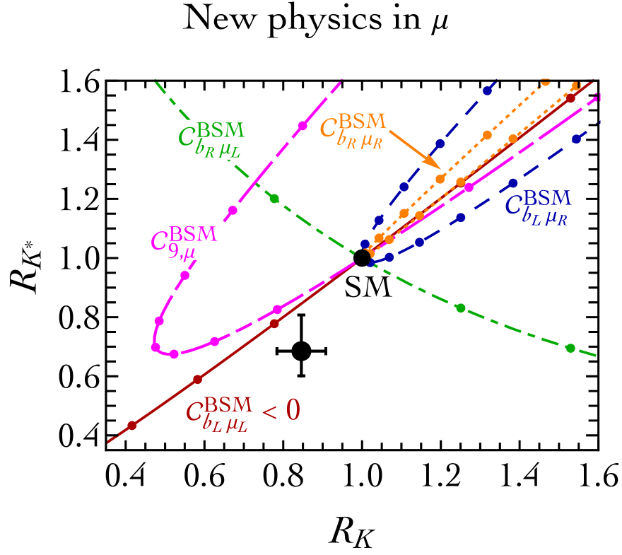
Refer to caption
Refer to caption
Figure 9: As in fig. 1, adding Moriond EW 2019 data about RKsubscript𝑅𝐾R_{K} and RKsubscript𝑅superscript𝐾R_{K^{*}}. Black: combination. Small dots on the theoretical predictions mark changes in steps of 111 of the corresponding coefficients.

6   Addendum: results presented at Moriond EW 2019

The LHCb collaboration presented a new measurement of the RKsubscript𝑅𝐾R_{K} ratio using a part of LHC run II data, and a revised analysis of run I data. The result [1]

RK|runIrevised=0.7170.071+0.083±0.017,RK|runII=0.9280.076+0.089±0.020,formulae-sequenceevaluated-atsubscript𝑅𝐾runIrevisedplus-or-minussubscriptsuperscript0.7170.0830.0710.017evaluated-atsubscript𝑅𝐾runIIplus-or-minussubscriptsuperscript0.9280.0890.0760.020R_{K}|_{\rm run~{}I}^{\rm revised}=0.717^{+0.083}_{-0.071}\pm 0.017,\qquad R_{K}|_{\rm run~{}II}=0.928^{+0.089}_{-0.076}\pm 0.020, (32)

is compatible both with the SM and with the previous result. The average is [1]

RK=BR(B+K+μ+μ)BR(B+K+e+e)=0.8460.054+0.060±0.015subscript𝑅𝐾BRsuperscript𝐵superscript𝐾superscript𝜇superscript𝜇BRsuperscript𝐵superscript𝐾superscript𝑒superscript𝑒plus-or-minussubscriptsuperscript0.8460.0600.0540.015R_{K}=\frac{{\rm BR}\left(B^{+}\to K^{+}\mu^{+}\mu^{-}\right)}{{\rm BR}\left(B^{+}\to K^{+}e^{+}e^{-}\right)}=0.846^{+0.060}_{-0.054}\pm 0.015 (33)

The central value is 2.52.52.5 standard deviations below unity. Furthermore, the Belle collaboration presented preliminary results about RKsubscript𝑅superscript𝐾R_{K^{*}}. Averaging over B0superscript𝐵0B^{0} and B+superscript𝐵B^{+}, the Belle result for the quantity defined in eq. (18) is [2].

RK[0.045,1.1]=0.520.26+0.36±0.05,RK[1.1,6]=0.960.29+0.45±0.11.formulae-sequencesubscript𝑅superscript𝐾0.0451.1plus-or-minussubscriptsuperscript0.520.360.260.05subscript𝑅superscript𝐾1.16plus-or-minussubscriptsuperscript0.960.450.290.11R_{K^{*}}[0.045,1.1]=0.52^{+0.36}_{-0.26}\pm 0.05,\qquad R_{K^{*}}[1.1,6]=0.96^{+0.45}_{-0.29}\pm 0.11. (34)

We combine these data with the LHCb data in eq. (2), which have smaller uncertainties. At the light of these new data we update our previous results concerning both the statistical significance of the anomaly as well the preferred chiral structure of the possible new physics. With the new data, the statistical significance of the anomaly remains essentially unchanged.

Assuming new physics in muons only, fig. 3 becomes fig. 10 and the best fits of eq. (22) become

CbLμLBSM=1.27±0.21CbRμLBSM=+0.50±0.19CbLμRBSM=0.27±0.32CbRμRBSM=+1.04±0.51withρ=(10.410.020.480.4110.250.380.020.2510.290.480.380.291).superscriptsubscript𝐶subscript𝑏𝐿subscript𝜇𝐿BSMplus-or-minus1.270.21superscriptsubscript𝐶subscript𝑏𝑅subscript𝜇𝐿BSMplus-or-minus0.500.19superscriptsubscript𝐶subscript𝑏𝐿subscript𝜇𝑅BSMplus-or-minus0.270.32superscriptsubscript𝐶subscript𝑏𝑅subscript𝜇𝑅BSMplus-or-minus1.040.51with𝜌10.410.020.480.4110.250.380.020.2510.290.480.380.291\begin{array}[]{rcl}C_{b_{L}\mu_{L}}^{\text{BSM}}&=&-1.27\pm 0.21\\ C_{b_{R}\mu_{L}}^{\text{BSM}}&=&+0.50\pm 0.19\\ C_{b_{L}\mu_{R}}^{\text{BSM}}&=&-0.27\pm 0.32\\ C_{b_{R}\mu_{R}}^{\text{BSM}}&=&+1.04\pm 0.51\\ \end{array}\qquad\hbox{with}\qquad\rho=\left(\begin{array}[]{cccc}1&-0.41&-0.02&-0.48\\ -0.41&1&-0.25&0.38\\ -0.02&-0.25&1&0.29\\ -0.48&0.38&0.29&1\\ \end{array}\right). (35)

Assuming new physics in muons and electrons, fig. 5 becomes fig. 11, table 1 and table 2 become table 8. See [3, 4, 5] for dedicated fits.

New physics in the muon sector
Wilson Best-fit 1-σ𝜎\sigma range χSM2χbest2subscriptsuperscript𝜒2SMsubscriptsuperscript𝜒2best\sqrt{\chi^{2}_{\rm SM}-\chi^{2}_{\rm best}}
coeff. ‘clean’ ‘HS’ all ‘clean’ ‘HS’ all ‘clean’ ‘HS’ all
CbLμLBSMsuperscriptsubscript𝐶subscript𝑏𝐿subscript𝜇𝐿BSMC_{b_{L}\mu_{L}}^{\rm BSM} 0.870.87-0.87 1.331.33-1.33 1.051.05-1.05 0.630.63-0.63 1.011.01-1.01 0.860.86-0.86 3.83.83.8 4.64.64.6 5.95.95.9
1.111.11-1.11 1.681.68-1.68 1.241.24-1.24
CbLμRBSMsuperscriptsubscript𝐶subscript𝑏𝐿subscript𝜇𝑅BSMC_{b_{L}\mu_{R}}^{\rm BSM} 0.560.560.56 0.730.73-0.73 0.290.29-0.29 1.051.051.05 0.400.40-0.40 0.030.030.03 1.11.11.1 2.12.12.1 0.90.90.9
0.070.070.07 1.031.03-1.03 0.580.58-0.58
CbRμLBSMsuperscriptsubscript𝐶subscript𝑏𝑅subscript𝜇𝐿BSMC_{b_{R}\mu_{L}}^{\rm BSM} 0.100.10-0.10 0.200.20-0.20 0.160.16-0.16 0.120.120.12 0.040.04-0.04 0.040.04-0.04 0.40.40.4 1.31.31.3 1.31.31.3
0.310.31-0.31 0.290.29-0.29 0.260.26-0.26
CbRμRBSMsuperscriptsubscript𝐶subscript𝑏𝑅subscript𝜇𝑅BSMC_{b_{R}\mu_{R}}^{\rm BSM} 0.410.41-0.41 0.410.410.41 0.260.260.26 0.080.080.08 0.610.610.61 0.470.470.47 0.80.80.8 1.71.71.7 1.11.11.1
0.910.91-0.91 0.180.180.18 0.040.040.04
New physics in the electron sector
Wilson Best-fit 1-σ𝜎\sigma range χSM2χbest2subscriptsuperscript𝜒2SMsubscriptsuperscript𝜒2best\sqrt{\chi^{2}_{\rm SM}-\chi^{2}_{\rm best}}
coeff. ‘clean’ ‘HS’ all ‘clean’ ‘HS’ all ‘clean’ ‘HS’ all
CbLeLBSMsuperscriptsubscript𝐶subscript𝑏𝐿subscript𝑒𝐿BSMC_{b_{L}e_{L}}^{\rm BSM} 1.011.011.01 0.150.150.15 0.790.790.79 1.351.351.35 0.690.690.69 1.051.051.05 3.73.73.7 0.30.30.3 3.53.53.5
0.710.710.71 0.390.39-0.39 0.550.550.55
CbLeRBSMsuperscriptsubscript𝐶subscript𝑏𝐿subscript𝑒𝑅BSMC_{b_{L}e_{R}}^{\rm BSM} 4.154.15-4.15 1.701.70-1.70 3.313.31-3.31 3.453.45-3.45 0.330.330.33 2.722.72-2.72 4.14.14.1 0.90.90.9 3.83.83.8
4.834.83-4.83 2.832.83-2.83 3.843.84-3.84
CbReLBSMsuperscriptsubscript𝐶subscript𝑏𝑅subscript𝑒𝐿BSMC_{b_{R}e_{L}}^{\rm BSM} 0.180.180.18 0.510.51-0.51 0.130.130.13 0.410.410.41 0.290.290.29 0.350.350.35 0.80.80.8 0.70.70.7 0.60.60.6
0.040.04-0.04 1.551.55-1.55 0.080.08-0.08
CbReRBSMsuperscriptsubscript𝐶subscript𝑏𝑅subscript𝑒𝑅BSMC_{b_{R}e_{R}}^{\rm BSM} 4.394.39-4.39 2.102.102.10 3.323.32-3.32 3.693.69-3.69 3.523.523.52 2.532.53-2.53 3.93.93.9 0.50.50.5 2.72.72.7
5.085.08-5.08 2.692.69-2.69 3.993.99-3.99
New physics in the muon sector (Vector Axial basis)
Wilson Best-fit 1-σ𝜎\sigma range χSM2χbest2subscriptsuperscript𝜒2SMsubscriptsuperscript𝜒2best\sqrt{\chi^{2}_{\rm SM}-\chi^{2}_{\rm best}}
coeff. ‘clean’ ‘HS’ all ‘clean’ ‘HS’ all ‘clean’ ‘HS’ all
C9,μBSMsuperscriptsubscript𝐶9𝜇BSMC_{9,\,\mu}^{\rm BSM} 0.890.89\rm-0.89 1.151.15-1.15 1.091.09-1.09 1.191.19-1.19 0.980.98-0.98 0.940.94-0.94 3.53.53.5 5.55.55.5 6.56.56.5
1.341.34-1.34 1.311.31-1.31 1.241.24-1.24
C10,μBSMsuperscriptsubscript𝐶10𝜇BSMC_{10,\,\mu}^{\rm BSM} 0.780.780.78 0.480.480.48 0.620.620.62 1.021.021.02 0.690.690.69 0.780.780.78 3.83.83.8 2.42.42.4 4.44.44.4
0.560.560.56 0.280.280.28 0.470.470.47
C9,μBSMsuperscriptsubscript𝐶9𝜇BSMC_{9,\,\mu}^{\prime{\rm BSM}} 0.170.17-0.17 0.240.24-0.24 0.220.22-0.22 0.040.040.04 0.150.15-0.15 0.150.15-0.15 0.80.80.8 1.71.71.7 1.91.91.9
0.390.39-0.39 0.370.37-0.37 0.330.33-0.33
C10,μBSMsuperscriptsubscript𝐶10𝜇BSMC_{10,\,\mu}^{\prime{\rm BSM}} 0.010.010.01 0.100.100.10 0.080.080.08 0.200.200.20 0.190.190.19 0.160.160.16 0.10.10.1 1.21.21.2 1.11.11.1
0.170.17-0.17 0.010.010.01 0.010.010.01
Table 8: As in table 1 and table 2, adding Moriond EW 2019 data about RKsubscript𝑅𝐾R_{K} and RKsubscript𝑅superscript𝐾R_{K^{*}}.
Refer to caption
Figure 10: As in fig. 3, adding Moriond EW 2019 data about RKsubscript𝑅𝐾R_{K} and RKsubscript𝑅superscript𝐾R_{K^{*}}.
Refer to caption
Figure 11: As in fig. 5, adding Moriond EW 2019 data about RKsubscript𝑅𝐾R_{K} and RKsubscript𝑅superscript𝐾R_{K^{*}}.

References

  • [1] LHCb collaboration, “Search for lepton-universality violation in B+K++superscript𝐵superscript𝐾superscriptsuperscriptB^{+}\to K^{+}\ell^{+}\ell^{-} decays” [arXiv:1903.09252]. Talk by T. Humair (LHCb collaboration) at the Moriond EW 2019 conference (slides).
  • [2] Talk by M. Prim (Belle collaboration) at the Moriond EW 2019 conference (slides).
  • [3] M. Algueró, B. Capdevila, A. Crivellin, S. Descotes-Genon, P. Masjuan, J. Matias, J. Virto, “Addendum: ”Patterns of New Physics in bs+𝑏𝑠superscriptsuperscriptb\to s\ell^{+}\ell^{-} transitions in the light of recent data”” [arXiv:1903.09578].
  • [4] A.K. Alok, A. Dighe, S. Gangal, D. Kumar, “Continuing search for new physics in bsμμ𝑏𝑠𝜇𝜇b\to s\mu\mu decays: two operators at a time” [arXiv:1903.09617].
  • [5] M. Ciuchini, A.M. Coutinho, M. Fedele, E. Franco, A. Paul, L. Silvestrini, M. Valli, “New Physics in bs+𝑏𝑠superscriptsuperscriptb\to s\ell^{+}\ell^{-} confronts new data on Lepton Universality” [arXiv:1903.09632].