Collisional Dynamics of Solitons in the Coupled $\cal{PT}$ Symmetric Nonlocal Nonlinear Schrödinger Equations

Abstract

We investigate the focussing coupled $\cal{PT}$ symmetric nonlocal nonlinear Schrödinger equation employing Darboux transformation approach. We find a family of exact solutions including pairs of Bright-Bright, Dark-Dark and Bright-Dark solitons in addition to solitary waves. We show that one can convert bright bound state onto a dark bound state in a two soliton solution by selectively finetuning the amplitude dependent parameter. We also show that the energy in each mode remains conserved unlike the celebrated Manakov model. We also characterize the behaviour of the soliton solutions in detail. We emphasize that the above phenomenon occurs due to the nonlocality of the model.

1 Introduction

Solitons are an important subject of study in both theoretical and experimental aspects in various fields, such as nonlinear optics, Bose-Einstein condensates, plasma physics and hydrodynamics. Nonlinear differential equation which describes these physical media gives rise to solitonic solutions. In the study of nonlinear wave propagation, by generating explicit soliton solutions, exactly solvable models play a pivotal role. There are many physically significant integrable systems which apply to diverse problems in nonlinear optics. In particular, the nonlinear Schrödinger equation (NLSE) and its coupled equation (CNLSE) have been most thoroughly investigated as integrable models, especially in nonlinear optics, where many species of solitons have been predicted [1]. Finding new integrable reductions of known nonlinear differential equations like NLSE or CNLSE is a new trend in the theory of integrable systems. This is motivated by the fact that, new integrable systems may give rise to new solutions. This, inturn, provides new ideas to proceed further to unearth significant results in future, and also open new avenues in the respective fields.

As mentioned above, recently Ablowitz and Musslimani proposed a new nonlocal NLSE [2]

$$\textit{i}q_{t}(x,t)=q_{xx}(x,t)+2gq(x,t)q^{\ast}(-x,t)q(x,t),$$ (1)

where, $q(x,t)$ is a complex valued function of real variables $x$ and $t$, and $g=\pm 1$ denotes, respectively, the focussing (+) and defocussing (-) cases. The above equation (1) is $\cal{PT}$ symmetric in the sense that the equation brings a self induced potential of the form $V(x,t)=q(x,t)q^{\ast}(-x,t)$ and satisfies the $\cal{PT}$ symmetric condition $V(x,t)=V^{\ast}(-x,t)$. In general, $\cal{PT}$ symmetric nonlinear Schrödinger systems should have linear potential term of the following form, namely

$$\textit{i}q_{t}(x,t)+q_{xx}(x,t)+V(x,t)q(x,t)+2\lvert q(x,t)\rvert^{2}q(x,t)=0.$$ (2)

This equation has been explored well in the last few years. For example: it includes the effect of nonlinearity on beam dynamics in $\cal{PT}$ symmetric potential [3], solitons in dual-core waveguides [4, 5], and Bragg solitons in $\cal{PT}$ symmetric potentials [6]. But, Ablowitz and Musslimani found the alternative way to fix the integrability in a nonlocal Schrödinger type equation by replacing the standard nonlinearity $\lvert q\rvert^{2}q$ with its $\cal{PT}$ symmetric counterpart $q(x,t)q^{\ast}(-x,t)q(x,t)$. Interestingly, in this study Ablowitz et al., have shown the new model given by Eq. (1) is fully integrable since it possesses linear Lax pair and infinite number of conserved quantities and nonlocal in the sense that the evolution of the field at transverse coordinate $x$ always requires the information from the opposite point $-x$ [2] .

As we mentioned before, new model reduction to the well known models provides us a chance to unearth new results like, the above new integrable model admits both bright and dark soliton solutions for the same nonlinear interaction $g<0$ with positive dispersion [7]. It is in contrast with the usual local NLSE, since it admits only bright and dark soltions for attractive ($g>0$) and repulsive ($g<0$) nonlinear interaction, respectively with positive dispersion. Realization of nonlocal nonlinearity is witnessed in many experiments such as, in diffusion of charge carriers, atoms, or molecules in atomic vapors [8, 9]. Also, it is witnessed in the study of BEC with a long-range interaction. The BEC with magnetic dipole-dipole forces was reported in [10] and occurred in the case of optical spatial solitons in a highly nonlocal medium [11]. It has been shown that nonlocal $\cal{PT}$ symmetric integrable equations can provide an ideal test bed for researchers to study and observe the ramification of nonlocality in optics. Due to the fact that, in optics, the paraxial equation of diffraction is mathematically isomorphic to the Schrödinger equation in quantum mechanics [12, 13, 14, 15], this analogy allowed observation of $\cal{PT}$ symmetry in optical waveguide structures and lattices [6, 16, 17]. This study of $\cal{PT}$ symmetric concepts in optics can also lead to alternative classes of optical structures and devices such as, non-Hermitian Bloch oscillations [18], simultaneous lasing-absorbing [19, 20], and selective lasing [21]. Finally, $\cal{PT}$-symmetric concepts have also been used in plasmonics [22], optical metamaterial [23, 24] and coherent atomic medium [25].

Motivated by the above significant results and unique dynamical behavior, we investigate the $\cal{PT}$-symmetric coupled nonlocal nonlinear Schrödinger equation (PTCNNLSE) in continuous media. Our analysis indicates that the $\cal{PT}$ symmetric CNLSE exhibits unique dynamics and features that one can convert bright bound state onto a dark bound state in a two soliton solution by selectively finetuning the amplitude-dependent parameter while the energy in each mode remains conserved unlike the Manakov model.

The plan of the paper is as follows. In section II, we present the mathematical (integrable) model governing the dynamics of nonlocal $\cal{PT}$ symmetric coupled nonlinear Schrödinger equation and its Lax pair and then derive the explicit soliton solution. In section III, we present the family of all solitonic solutions generated from the general solution obtained in section II. In section IV, we discuss the collisional dynamics of solitons and the mechanism which involves the conversion of bright to dark bound state. The results are then summarized in section V.

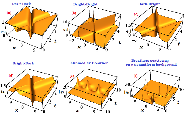
Figure 1: Families of exact two soliton solutions for the choice of parameter $\alpha_{1}=1,\alpha_{2}=0.5,a=-4,c=-1,b=0,d=0,a_{1}=8,\zeta_{1}=0,\eta_{1}=0.25\pi$ and manipulation of amplitude dependent parameter $b_{1}$ leads to cases (a) dark-dark for $b_{1}=7$, (b) bright-bright for $b_{1}=3.9$, (c) dark-bright for $b_{1}=2.8$, (d) bright-dark for $b_{1}=5$ and special cases like oscillatory solutions, namely (e) Akhmediev breather and (f) the difference between the background levels for the choice of parameter selectively chosen to achieve $J_{1}=-1(<0)$)

2 Coupled $\cal{PT}$ symmetric nonlocal NLSE

Let us consider, the coupled $\cal{PT}$ symmetric nonlocal NLSE of the following form,

$$\textit{i}\frac{\partial q_{1}(x,t)}{\partial t}+\frac{1}{2}\frac{\partial^{2}q_{1}(x,t)}{\partial x^{2}}+[q_{1}(x,t)q_{1}^{\ast}(-x,t)+q_{2}(x,t)q_{2}^{\ast}(-x,t)]q_{1}(x,t) =0,$$ (3a)

$$\textit{i}\frac{\partial q_{2}(x,t)}{\partial t}+\frac{1}{2}\frac{\partial^{2}q_{2}(x,t)}{\partial x^{2}}+[q_{1}(x,t)q_{1}^{\ast}(-x,t)+q_{2}(x,t)q_{2}^{\ast}(-x,t)]q_{2}(x,t) =0,$$ (3b)

where, $q_{j}(x,t)\,(j=1,2)$ are the two complex field amplitudes. This equation is also a non-Hermitian $\cal{PT}$ symmetric system in the sense that the self-induced potential $V(x,t)=q_{1}(x,t)q_{1}^{\ast}(-x,t)+q_{2}(x,t)q_{2}^{\ast}(-x,t)$ satisfies the $\cal{PT}$ symmetric condition $V(x,t)=V^{\ast}(-x,t)$. It is worth mentioning here, that Eq. (3) is nonlocal, i.e., the evolution of the field variables $(q_{1}(x,t),q_{2}(x,t))$ at the transverse coordinate $x$ always requires information from the opposite point $-x$. The above coupled Eqs. (3a) and (3b) admit the following Lax pair

$$\Phi_{x}+{\bf U}\Phi= 0,$$ (4a)

$$\Phi_{t}+{\bf V}\Phi= 0,$$ (4b)

where $\Phi=(\phi_{1},\phi_{2},\phi_{3})^{T}$ is a three-component Jost function,

$${\bf U}=\begin{pmatrix}2i\lambda&iq_{1}(x,t)&iq_{2}(x,t)\\ iq^{\ast}_{1}(x,t)&0&0\\ iq^{\ast}_{2}(x,t)&0&0\end{pmatrix},\;\;\;{\bf V}=\begin{pmatrix}{\bf V}_{11}&{\bf V}_{12}&{\bf V}_{13}\\ {\bf V}_{21}&{\bf V}_{22}&{\bf V}_{23}\\ {\bf V}_{31}&{\bf V}_{32}&{\bf V}_{33}\end{pmatrix},$$ (5)

with

$${\bf V}_{11}= \textit{i}\lambda^{2}-\frac{1}{2}\textit{i}\left[q_{1}(x,t)q^{\ast}_{1}(x,t)+q_{2}(x,t)q^{\ast}_{2}(x,t)\right],$$

$${\bf V}_{12}= \textit{i}\lambda q_{1}(x,t)+\frac{1}{2}q^{\ast}_{1x}(x,t),\,\,{\bf V}_{13}=\textit{i}\lambda q_{2}(x,t)+\frac{1}{2}q^{\ast}_{2x}(x,t),$$

$${\bf V}_{21}= \textit{i}\lambda q^{\ast}_{1}(x,t)-\frac{1}{2}q^{\ast}_{1x}(x,t),$$

$${\bf V}_{22}= -\textit{i}\lambda^{2}+\frac{1}{2}\textit{i}\left[q_{1}(x,t)q^{\ast}_{1}(x,t)\right],$$

$${\bf V}_{23}= -\frac{\textit{i}}{2}q_{1}(x,t)q^{\ast}_{1}(x,t),$$

$${\bf V}_{31}= \textit{i}\lambda q^{\ast}_{2}(x,t)-\frac{1}{2}q^{\ast}_{2x}(x,t),\,\ {\bf V}_{32}=-\frac{\textit{i}}{2}q_{2}(x,t)q^{\ast}_{2}(x,t),$$

$${\bf V}_{32}= -\frac{\textit{i}}{2}q_{2}(x,t)q^{\ast}_{2}(x,t),$$

$${\bf V}_{33}= -\textit{i}\lambda^{2}+\frac{1}{2}\textit{i}\left[q_{2}(x,t)q^{\ast}_{2}(x,t)\right],$$

where $\lambda$ is the spectral parameter. The compatibility condition (or the Zero Curvature condition)${\bf U}_{t}-{\bf V}_{x}+[{\bf U},{\bf V}]=0$ generates the classical local coupled NLS equation of the following form

$$\textit{i}\frac{\partial q_{1}}{\partial t}+\frac{1}{2}\frac{\partial^{2}q_{1}}{\partial x^{2}}+[q_{1}(x,t)q_{1}^{\ast}(x,t)+q_{2}(x,t)q_{2}^{\ast}(x,t)]q_{1}(x,t) =0,$$ (6)

$$\textit{i}\frac{\partial q_{2}}{\partial t}+\frac{1}{2}\frac{\partial^{2}q_{2}}{\partial x^{2}}+[q_{1}(x,t)q_{1}^{\ast}(x,t)+q_{2}(x,t)q_{2}^{\ast}(x,t)]q_{2}(x,t) =0.$$ (7)

We then employ the strategy proposed by Ablowitz and Mussilimani [2] and sustain the integrability (or the lax-pair) by replacing the nonlinear interaction term $[|q_{1}|^{2}+|q_{2}|^{2}]q_{1}$ and $[|q_{1}|^{2}+|q_{2}|^{2}]q_{2}$ in the above coupled equations by their $\cal{PT}$ symmetric counterparts, namely, $[q_{1}q_{1}^{\ast}(-x,t)+q_{2}q_{2}^{\ast}(-x,t)]q_{1}$ and $[q_{1}q_{1}^{\ast}(-x,t)+q_{2}q_{2}^{\ast}(-x,t)]q_{2}$, to obtain the ${\cal PT}$ symmetric coupled nonlocal NLSE given by Eqs. (3a) and (3b).

As mentioned in the introduction, this new integrable PTCNNLSE equation admits both bright and dark solitons for the same nonlinearity unlike the conventional Manakov model (CNLSE). The nonsingular bright soliton solution of Eq.(3), of the following form (was constructed by following the details given by Liming et al.,[29])

$$q_{1}^{(1)}= 2a\sin(\theta)\mathrm{sech}(2ax+\textit{i}k){\rm e}^{2\textit{i}a^{2}t},$$ (8a)

$$q_{2}^{(1)}= 2a\cos(\theta)\mathrm{sech}(2ax+\textit{i}k){\rm e}^{2\textit{i}a^{2}t},$$ (8b)

where $a,k,\theta\in\Re$, $k\neq\pi$. The nonsingular single dark solutions for Eqs. (3) are

$$q_{1}^{(1)}= a\sin(\theta)\tanh(ax+\textit{i}k){\rm e}^{-\textit{i}a^{2}t},$$ (9a)

$$q_{2}^{(1)}= a\cos(\theta)\tanh(ax+\textit{i}k){\rm e}^{-\textit{i}a^{2}t},$$ (9b)

where $a,k,\theta\in\Re$, $k\neq\pi$ with,

The bright and dark soliton solutions given by eqs.(8) and (9) are identical to the one generated for PT symmetric scalar nonlocal NLS equation [7] and the details of the derivation of the bright and dark solitons are found in ref.[29].

To understand the impact of nonlocal interaction, we need higher order soliton solutions. For that, we employ Darboux transformation approach to construct the two soliton solutions of the following form:

$$q_{k}^{(2)}=\alpha_{k}\left[\frac{\cosh(\zeta_{1})\cosh(A-2\textit{i}\eta_{1})+\cos(\eta_{1})\cosh(B+2\zeta_{1})}{\cosh(\zeta_{1})\cosh(A)+\cos(\eta_{1})\cosh(B)}\right]{\rm e}^{\textit{i}\phi t}$$ (10)

$$A= X_{1}+X_{2}-\zeta_{1}+a_{1},\;\;B=-X_{1}+X_{2}+\textit{i}\eta_{1}-\textit{i}b_{1},$$

$$X_{1}= \textit{i}\sqrt{J_{1}}\sinh\left(\zeta_{1}+\textit{i}\eta_{1}\right)\left(x+\sqrt{J_{1}}\cosh\left(\zeta_{1}+\textit{i}\eta_{1}\right)t\right),$$

$$X_{2}= \textit{-i}\sqrt{J_{1}}\sinh\left(\zeta_{1}-\textit{i}\eta_{1}\right)\left(-x+\sqrt{J_{1}}\cosh\left(\zeta_{1}-\textit{i}\eta_{1}\right)t\right),$$

$$J_{1}= -\left(a\alpha_{1}^{2}+2b\alpha_{1}\alpha_{2}+d\alpha_{2}^{2}\right),$$ (11)

where $\zeta_{1}$ and $\eta_{1}$ are spectral parameters and $\alpha_{1},\beta_{1},a_{1},b_{1},a,b,d$ are real arbitrary parameters.

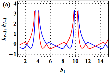
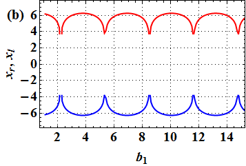
Figure 2: (a) Blue and Red lines show the heights of the two solitons $h_{r}$ and $h_{l}$, respectively, with respect to the uniform background of one. (b) The two solitons locations $x_{r}$ and $x_{l}$.

Figure 3: Density plot of $|q_{1}|$ showing the conversion of Dark-Dark soliton into Bright-Bright, Dark-Bright (or) Bright-Dark by manipulating the parameter $b_{1}$.

3 Family of exact solutions

Equation (10) corresponds to a host of exact solitonic solutions which can be obtained for specific values of the parameters. By inspection, we found the group of solutions containing: i) a pair of solitons, ii) a solitonic oscillatory wave, iii) Akhmedeiv breather. All these solutions were on a uniform background. Interestingly, we found that these solutions exist also on a nonuniform background.

The pair of solitons solutions include Bright-Bright (BB), Dark-Dark (DD), Bright-Dark (BD), and Dark-Bright (DB) solitons. The main features of these solutions are obtained by noticing that the denominator of Eq. (10) contains two peaks which result in two soliton profiles. Therefore, the locations of the two solitons are determined by the roots of the first derivative of the denominator of Eq. (10), namely

$$x_{r}= \Re\left[J_{1}^{-1/2}\cosh^{-1}\left(\frac{A_{1}}{A_{2}}\right)\csc(\eta_{1})\right],$$

where

$$A_{1}= \sqrt{\cos(\eta_{1})\left(\cos(\eta_{1})-\cos(b_{1}-\eta_{1})\cosh(a_{1})\right)}$$

$$A_{2}= \sqrt{1+\cos(2\eta_{1})}$$

$$x_{l}= -x_{r}$$

where $x_{r}$ and $x_{l}$ are the locations of the soliton on the right and left of the origin. The corresponding amplitudes of the two solitons, $h_{r}$ and $h_{l}$, are then calculated by substituting these expressions back in $q_{1}$. The separation between the two solitons and their peaks are thus determined by the parameters $J_{1}$, $a_{1}$, $\eta_{1}$, and $b_{1}$. In Fig.1, we show the whole family of independent solutions of Eq. (10). In addition to the pairs of soliton solutions, we show an oscillatory solution, for $J_{1}<0$, identified as the Akhmedeiv breather [26, 27] shown in Fig.1(e). Furthermore, we found that the parameter $\zeta_{1}$ represents the separation between the background levels between the two sides of the $x$-axis. This is obtained by taking the limits $\lim_{x\rightarrow\pm\infty}|q_{1}|$ which will be $\exp{(2\zeta_{1})}$ for the right side and $\exp{(-2\zeta_{1})}$ for the left side. Therefore the difference between the two background levels equals $\exp{(2\zeta_{1})}-\exp{(-2\zeta_{1})}$. This case is shown Fig.1(f).

Remarkably, we found that all kinds of pair of soliton solutions can be obtained by manipulating one parameter, namely $b_{1}$. Fixing all other parameters, we plot in Fig.2 the solitons locations and their peak values with respect to the background. This figure gives the values of $b_{1}$ where we have dark-bright ($b_{1}=2.8$), bright-dark ($b_{1}=4.3$), bright-bright ($b_{1}=3.9$) and dark-dark ($b_{1}=5.0$) solitons. The separation between the two solitons is controlled most sensitively by $a_{1}$.

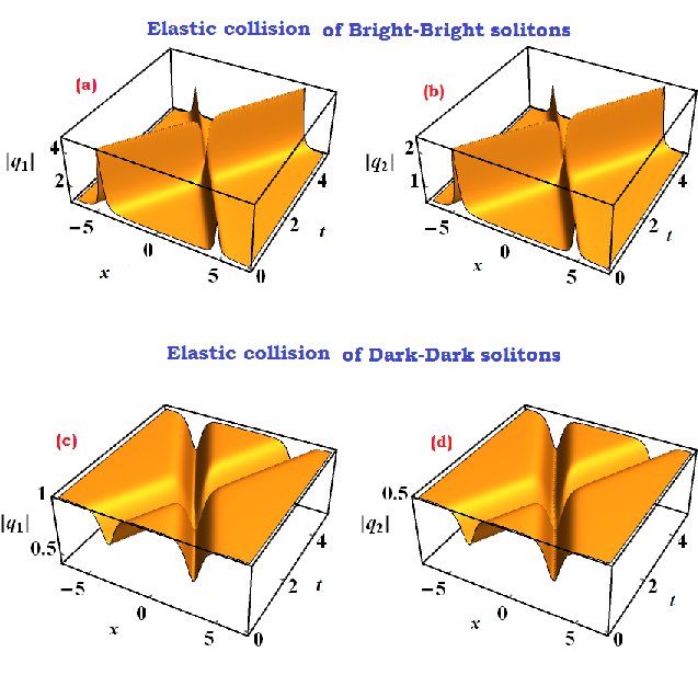
Figure 4: Density plots of $\lvert q_{1}\rvert$ and $\lvert q_{2}\rvert$ showing elastic collisions of (a,b) Bright and (c,d) Dark solitons for the choice of parameters $\alpha_{1}=1,\alpha_{2}=0.5,a=-4,b=-1,b=0,d=0,a_{1}=8,\zeta_{1}=0$ with $\eta_{1}=0.14\pi,b_{1}=3.8$ and $\eta_{1}=0.25\pi,b_{1}=7$ for bright and dark solitons respectively

4 Collisional Dynamics of Solitons and their Conversion

As we mentioned before, the classical (local) coupled nonlinear Schrödinger equation admits only bright and dark soliton solutions when their interatomic interaction were attractive or repulsive, respectively. Unlike the usual behaviour, the study of this parity-time symmetry in nonlocal integrable coupled NLS equation surprisingly admits both bright and dark solitons for the same nonlinearity. So, we step up our investigation and show that one can convert the bright mode into a dark mode by selectively finetuning the amplitude-dependent parameter in a two soliton solution. In other words, one can convert the bright-bright soliton into bright-dark or dark-dark by finetunig the amplitude-dependent parameter without violating the integrability. The conversion of soliton bound states with respect to parameter $b_{1}$ at time $t=0$, is shown in Fig. 3. The evolution of the dark-dark soliton is as shown in Fig. 1(a) for the choice of parameter $b_{1}$=7. One can accomplish the conversion of dark-dark soliton into bright-bright soliton as shown in Fig.3 and the corresponding evolution is as shown in Fig.1(b) by tuning the amplitude-dependent parameter to $b_{1}$=3.9. The choice of parameter $b_{1}$=2.8 and $b_{1}=5$ lead to the conversion of bright-bright to dark-bright and bright-dark solitons, respectively, as shown in Fig. 3 and the respective evolution is shown in Fig.1(c) and (d) respectively.

It is interesting to notice, as shown in Fig. 1(f), that in the case when the levels of the background are unequal, the solitons reflect off the boundary between the two values of the background. This is in contrast with the uniform background case where the solitons transmit through each other and continue their trajectory in a straight path.

Being an exact solution, the two soliton solution conserves the energy. Therefore, solitons conversion between the different members of the family of solutions (BB, DD, BD, and DB) is guaranteed to conserve energy. We confirm this viewpoint by showing the elastic collision of bright and dark solitons in fig.4 (a,b) and (c,d) respectively. It is only with nonlocality that such combinations of solitons and their conversion exists.

5 Conclusion

In this paper, we investigated $\cal{PT}$ symmetric CNLS equation employing Darboux transformation to generate a family of exact solitonic solutions including a combination of bright and dark solitons in addition to breathers both on a uniform and nonuniform backgrounds. We have shown that one can convert a bright bound state into a dark bound state in a mixed soliton solution by manipulating the free (or arbitrary) parameter associated with the system. We believe that the above phenomenon occurs due to the nonlocal nature of the dynamical system. A refinement on the present model would be incorporating $\cal{PT}$ symmetry through a potential while retaining the traditional cubic nonlinear term. Such a model is more realistic and may be tested experimentally, which we leave to future study.

6 Acknowledgements:

UAK and PSV acknowledge the support of UAE University through the grant UAEU-UPAR(7) and UAEU-UPAR(4). RR wishes to acknowledge the financial assistance received from Department of Atomic Energy-National Board for Higher Mathematics (DAE-NBHM) (No. NBHM/R.P.16/2014) and Council of Scientific and Industrial Research (CSIR) (No. 03(1323)/14/EMR-II) for the financial support in the form Major Research Projects. LL acknowledge the financial support received from National Natural Science Foundation of China (Contact No. 11401221). PSV and RR wish to acknowledge the technical discussion with Prof. D-S. Wang, Beijing Information Science and Technology University, Beijing, China.

7 Appendix: Lax pair and Darboux transformation of the system given by eq.(3)

For nonlinear partial differential equations, Darboux transformation [28] is applied in an indirect manner. One starts by finding a linear system of equations for an auxiliary field ${\bf\Psi}$ in the form ${\bf\Psi}_{x}$ = ${\bf U.\Psi}$ and ${\bf\Psi}_{t}={\bf V.\Psi}$, where ${\bf\Psi}$, ${\bf U}$ and ${\bf V}$ are $3\times 3$ matrices. The pair of matrices ${\bf U}$ and ${\bf V}$, known as the Lax pair, are functionals of the solution of the differential equation. The consistency condition of the linear system, ${\bf\Psi}_{xt}={\bf\Psi}_{tx}$, should be equivalent to the differential equation. The linear system and hence its consistency condition are covariant under the Darboux transformation. Therefore, applying the Darboux transformation on the linear system results in a new consistency condition which is equivalent to a new differential equation that is covariant with the old one. The new differential equation is satisfied by a new solution. In the following two subsections, we describe this procedure in a more detailed manner.

7.1 Darboux transformation

Consider the general form of nonlinear partial differential equation

$$F_{k}[Q(x,t),Q^{\ast}(x,t),Q_{t}(x,t),Q_{xx}(x,t)]=0,\;\;(Q(x,t)=q_{k}(x,t)\;\&\;k=1,2).$$ (12)

The auxiliary field is represented by a $3\times 3$ matrix:

$${\bf\Psi}=\begin{pmatrix}\psi_{1}(x,t)&\psi_{2}(x,t)&\psi_{3}(x,t)\\ \phi_{1}(x,t)&\phi_{2}(x,t)&\phi_{3}(x,t)\\ \chi_{1}(x,t)&\chi_{2}(x,t)&\chi_{3}(x,t)\end{pmatrix}.$$ (13)

The linear system of equations of the auxiliary field is formally written as an expansion in powers of the constant eigenvalue matrix

$${\bf\Lambda} =\begin{pmatrix}\lambda_{1}&0&0\\ 0&\lambda_{2}&0\\ 0&0&\lambda_{3}\end{pmatrix},$$ (14)

as follows

$${\bf\Psi}_{x} ={\bf U_{0}}{\bf\Psi}+{\bf U_{1}}{\bf\Psi}{\bf\Lambda},$$ (15a)

$${\bf\Psi}_{t} ={\bf V_{0}}{\bf\Psi}+{\bf V_{1}}{\bf\Psi}{\bf\Lambda}+{\bf V_{2}}{\bf\Psi}{\bf\Lambda}^{2},$$ (15b)

where,

$${\bf U_{0}}=\begin{pmatrix}0&q_{1}(x,t)&q_{2}(x,t)\\ -r_{1}(x,t)&0&0\\ -r_{2}(x,t)&0&0\end{pmatrix},\;\;\;{\bf U_{1}}=\begin{pmatrix}1&0&0\\ 0&-1&0\\ 0&0&-1\end{pmatrix},$$

$${\bf V_{0}}=\frac{\textit{i}}{2}\begin{pmatrix}q_{1}(x,t)r_{1}(x,t)+q_{2}(x,t)r_{2}(x,t)&q_{1x}(x,t)&q_{2x}(x,t)\\ r_{1x}(x,t)&-q_{1}(x,t)r_{1}(x,t)&-q_{2}(x,t)r_{1}(x,t)\\ r_{2x}(x,t)&-q_{1}(x,t)r_{2}(x,t)&-q_{2}(x,t)r_{2}(x,t)\end{pmatrix},$$

$${\bf V_{1}} =\begin{pmatrix}0&-q_{1}(x,t)&-q_{2}(x,t)\\ r_{1}(x,t)&0&0\\ r_{2}(x,t)&0&0\end{pmatrix},\;\;\;{\bf V_{2}}=\mathrm{i}\begin{pmatrix}1&0&0\\ 0&-1&0\\ 0&0&-1\end{pmatrix},$$

along with the transformation on the complex conjugates

$$r_{1}(x,t) =q_{1}^{\ast}(-x,t),$$

$$r_{2}(x,t) =q_{2}^{\ast}(-x,t).$$

The consistency condition ${\bf\Psi}_{xt}={\bf\Psi}_{tx}$ leads to

$${\bf U_{0}}_{t}-{\bf V_{0}}_{x}+\Big{[}{\bf U_{0}},{\bf V_{0}}\Big{]}={\bf 0},$$ (16a)

$${\bf U_{1}}_{t}-{\bf V_{1}}_{x}+\Big{[}{\bf U_{0}},{\bf V_{1}}\Big{]}+\Big{[}{\bf U_{1}},{\bf V_{0}}\Big{]}={\bf 0},$$ (16b)

$${\bf U_{2}}_{t}-{\bf V_{2}}_{x}+\Big{[}{\bf U_{0}},{\bf V_{2}}\Big{]}+\Big{[}{\bf U_{1}},{\bf V_{1}}\Big{]}+\Big{[}{\bf U_{2}},{\bf V_{0}}\Big{]}={\bf 0},$$ (16c)

$$\Big{[}{\bf U_{1}},{\bf V_{2}}\Big{]}+\Big{[}{\bf U_{2}},{\bf V_{1}}\Big{]}={\bf 0},$$ (16d)

$$\Big{[}{\bf U_{2}},{\bf V_{2}}\Big{]}={\bf 0}.$$ (16e)

These equations are obtained by equating the coefficients ${\bf\Lambda^{0}},{\bf\Lambda^{1}},{\bf\Lambda^{2}}$ and ${\bf\Lambda^{3}}$ in ${\bf\Psi}_{xt}$ to the corresponding ones in ${\bf\Psi}_{tx}$. The matrices ${\bf U_{0}}$, ${\bf V_{0}}$ are the Lax pair of model equation (3) & the consistency condition, eq.(16)(a) is equivalent to equations (6,7).

Considering the following version of Darboux transformation

$${\bf\Psi}[1]={\bf\Psi}{\bf\Lambda}-{\bf\sigma\Psi},$$ (17)

where, ${\bf\Psi}[1]$ is the transformed field and ${\bf\sigma}={\bf\Psi_{0}}.{\bf\Lambda}.{\bf\Psi_{0}^{-1}}$. where ${\bf\Psi_{0}}$ is the known solution of the linear system given by (15). To determine the solution, the coefficients of the linear system should be known explicitly. These coefficients are functionals of the solution of the differential equation $Q$. Thus, determining the coefficients of the linear system requires knowing an exact solution of the differential equation. This solution is known as the seed solution, which we denote here by $Q_{0}$. It is in the very nature of the Darboux transformation method that new exact solutions are only obtained from other exact solutions. The transformed field ${\bf\Psi}[1]$ is required to be a solution of a linear system that is covariant with the system (15), namely

$${\bf\Psi}[1]_{x} ={\bf U_{0}}[1]{\bf\Psi}[1]+{\bf U_{1}}[1]{\bf\Psi}[1]{\bf\Lambda},$$ (18a)

$${\bf\Psi[1]}_{t} ={\bf V_{0}}[1]{\bf\Psi}[1]+{\bf V_{1}}[1]{\bf\Psi}[1]{\bf\Lambda}+{\bf V_{2}}[1]{\bf\Psi}[1]{\bf\Lambda}^{2}.$$ (18b)

Requiring the system given by Eqs.(18) to be covariant with the system of Eqs. (15) leads to the consistency condition

$${\bf U_{0}}[1]_{t}-{\bf V_{0}}[1]_{x}+\Big{[}{\bf U_{0}}[1],{\bf V_{0}}[1]\Big{]}={\bf 0},$$ (19)

this is covariant with Eq. (15)(a). Similar to model equation(3), this new consistency condition will be equivalent to a differential equation and it must be co variant with equation(3).

$${\bf U_{0}}[1]_{t}-{\bf V_{0}}[1]_{x}+\Big{[}{\bf U_{0}}[1],{\bf V_{0}}[1]\Big{]}=\begin{pmatrix}0&F_{1}&F_{2}\\ F_{1}^{\ast}&0&0\\ F_{2}^{\ast}&0&0\end{pmatrix}=0,$$ (20)

and the above new lax condition must be equivalent to the same model equation under consideration.This means that $Q[1]$ is the new solution of the same differential equation for which $Q_{0}$ is the seed solution.

To find ${\bf U_{0}}[1]$ or ${\bf V_{0}}[1]$ and hence $Q[1]$, we substitute for ${\bf\Psi}[1]$ from eq.(17) in eq.(18) using eqs.(15) and then equate the $\Lambda$ powers to zero to get

$${\bf U_{0}}[1] ={\bf\sigma}{\bf U_{0}}{\bf\sigma}^{-1}+{\bf\sigma}_{x}{\bf\sigma}^{-1},$$ (21)

$${\bf U_{0}}[1] ={\bf U_{0}}+[{\bf U_{1}},{\bf\sigma}].$$ (22)

The new solution $Q[1]$ can be calculated using either of these two equations which can be shown to be equivalent. Notice that the quantities on the right-hand side are calculated using the seed solution $Q_{0}$.

To summarize, a nonlinear differential equation can be solved with the Darboux transformation method by first finding an exact (seed) solution, $Q_{0}$, to the differential equation and finding a linear system for an auxiliary field ${\bf\Psi}$ that is associated with the differential equation through its consistency condition. Using the seed solution, a solution of the linear system, ${\bf\Psi_{0}}$, is found. The linear system is then transformed into a new one via the Darboux transformation. Thus, the coefficients of the new linear system which are functionals of the new solution of the differential equation, $Q[1]$ will be related to the coefficients of the original linear system which are functionals of $Q_{0}$. This relation gives the new solution $Q[1]$ in terms of the seed solution $Q_{0}$. This procedure will be further illustrated with our specific example in the following Section.

7.2 Soliton solutions

The values for the lax pair matrices ${\bf U_{0,1,2}}$ and ${\bf V_{0,1,2}}$ are derived by trial and error method and their exact forms are given above. In the following, we consider two cases, namely zero and non-zero seed solutions. With zero seed, we obtain the fundamental solitons while with the non-zero seed, we obtain higher order solitons.

7.2.1 Zero seed

One can depart from two different paths to derive soliton solutions in Darboux transformation. The first choice is to feed the field variables $q_{1}(x,t)$ and $q_{2}(x,t)$ to be zero and use lax pair matrices and adopt the procedure enumerated above to obtain,

$$\left(\begin{array}[]{ccc}C_{11}e^{i\left(\lambda_{1}x-\lambda_{1}^{2}t\right)}&C_{12}e^{i\left(\lambda_{2}x-\lambda_{2}^{2}t\right)}&C_{13}e^{i\left(\lambda_{3}x-\lambda_{3}^{2}t\right)}\\ C_{14}e^{-i\left(\lambda_{1}x-\lambda_{1}^{2}t\right)}&C_{15}e^{-i\left(\lambda_{2}x-\lambda_{2}^{2}t\right)}&C_{16}e^{-i\left(\lambda_{3}x-\lambda_{3}^{2}t\right)}\\ C_{17}e^{-i\left(\lambda_{1}x-\lambda_{1}^{2}t\right)}&C_{18}e^{-i\left(\lambda_{2}x-\lambda_{2}^{2}t\right)}&C_{19}e^{-i\left(\lambda_{3}x-\lambda_{3}^{2}t\right)}\\ \end{array}\right),$$ (26)

which leads to the general one soliton solution of the following form

$$q_{k}^{(1)}(x,t)=\frac{2i(C_{11}(A_{1k}(\lambda_{1}-\lambda_{2})-A_{2k}(\lambda_{1}-\lambda_{3}))+A_{3k}(\lambda_{2}-\lambda_{3}))}{C_{13}B_{1k}-C_{12}B_{2k}+C_{11}B_{3k}},$$ (27)

where,

$$A_{11} =C_{12}C_{19}e^{2i((\lambda_{1}+\lambda_{2})x+\lambda_{3}^{2}t)},A_{21}=C_{13}C_{18}e^{2i((\lambda_{1}+\lambda_{3})x+\lambda_{2}^{2}t)},A_{31}=C_{12}C_{13}C_{17}e^{2i((\lambda_{2}+\lambda_{3})x+\lambda_{1}^{2}t)},$$

$$B_{11} =(C_{15}C_{17}-C_{14}C_{18})e^{2i(\lambda_{3}x+(\lambda_{1}^{2}+\lambda_{2}^{2})t)},\;B_{21}=(C_{16}C_{17}-C_{14}C_{19})e^{2i(\lambda_{2}x+(\lambda_{1}^{2}+\lambda_{3}^{2})t)},$$

$$B_{31} =(C_{16}C_{18}-C_{15}C_{19})e^{2i(\lambda_{1}x+(\lambda_{2}^{2}+\lambda_{3}^{2})t)},\;A_{12}=C_{12}C_{16}e^{2i((\lambda_{1}+\lambda_{2})x+\lambda_{3}^{2}t)},$$

$$A_{22} =C_{13}C_{15}e^{2i((\lambda_{1}+\lambda_{3})x+\lambda_{2}^{2}t)},\;A_{32}=C_{12}C_{13}C_{14}e^{2i((\lambda_{2}+\lambda_{3})x+\lambda_{1}^{2}t)},$$

$$B_{12} =-B_{11},\;B_{22}=-B_{21},\;B_{32}=-B_{31}.$$

Choosing the parameters $\lambda_{2}=\textit{i}\lambda_{3}$, $\lambda_{3}=\textit{i}a$, $\lambda_{1}=-\textit{i}a$ with $C_{11}=\textit{i}(-C_{15}C_{17}+C_{14}C_{18})/\sqrt{C_{15}^{2}+C_{18}^{2}}$, $C_{13}=\textit{i}(-C_{16}C_{18}+C_{15}C_{19})/\sqrt{C_{15}^{2}+C_{18}^{2}}$, $Re[\lambda_{1}]=Re[\lambda_{2}]=0$, $C_{15}\neq-C_{18}$, $(-C_{15}C_{17}+C_{14}C_{18})\neq 0$, $(-C_{16}C_{18}+C_{15}C_{19})\neq 0$ with $C_{15}^{2}+C_{18}^{2}=1$, one only needs to choose the constants suitably to derive the nonsingular bright solution given by equation (8), where $a,k$ are real arbitrary parameters.

7.2.2 Non-zero seed

We depart from the zero seed and choose the seed solution of the following form

$$q_{1}(x,t) =\alpha_{1}e^{i\phi t}$$ (29a)

$$q_{2}(x,t) =\alpha_{2}e^{i\phi t}$$ (29b)

where,$\phi=a\alpha_{1}^{2}+d\alpha_{2}^{2}+2b\alpha_{1}\alpha_{2}$ and $\alpha_{1}$, $\alpha_{2}$ $a,b,d$ are real free parameters and follow the procedure mentioned above so that the fundamental solution becomes

$$\Psi_{i}=JL_{i}E_{i},\,\,J=\mathrm{diag}(1,\textit{e}^{\textit{i}\phi},\textit{e}^{\textit{i}\phi}),$$

where

$$L_{i}=\begin{bmatrix}1&1&0\\[8.0pt] {\displaystyle\frac{\alpha_{1}}{\xi_{i,1}}}&{\displaystyle\frac{\alpha_{1}}{\xi_{i,2}}}&\beta_{1}\\[10.0pt] {\displaystyle\frac{\alpha_{2}}{\xi_{i,1}}}&{\displaystyle\frac{\alpha_{2}}{\xi_{i,2}}}&\beta_{2}\\ \end{bmatrix},\,\,E_{i}=\mathrm{diag}\left(c_{i,1}\textit{e}^{\theta_{i,1}},c_{i,2}\textit{e}^{\theta_{i,2}},c_{i,3}\right)$$

and

$$\begin{split}\theta_{i,1}(x,t)=&\textit{i}\xi_{i,1}\left(x+\frac{1}{2}\xi_{i,1}t\right),\,\,\theta_{i,2}(x,t)=\textit{i}\xi_{i,2}\left(x+\frac{1}{2}\xi_{i,2}t\right),\\ \beta_{1}=&-(b\alpha_{{1}}+d\alpha_{{2}}-\textit{i}c\alpha_{{1}}),\,\,\beta_{2}=a\alpha_{{1}}+b\alpha_{{2}}+\textit{i}c\alpha_{{2}},\\ \xi_{i,1}=&\lambda_{i}+\sqrt{\phi+\lambda_{i}^{2}},\,\,\xi_{i,2}=\lambda_{i}-\sqrt{\phi+\lambda_{i}^{2}}.\end{split}$$

Following the same procedure described above, one can obtain the general soliton solution of the following form

$$q_{k}[1]=\alpha_{k}\left[1+\frac{{\displaystyle\sum_{l=1}^{2}\sum_{m=1}^{2}\frac{c_{1,l}^{*}c_{1,m}{\rm e}^{\theta_{1,l}^{*}(-x,t)+\theta_{1,m}(x,t)}}{\xi_{1,m}}+c_{1,3}\beta_{k}\sum_{l=1}^{2}c_{1,l}^{*}{\rm e}^{\theta_{1,l}^{*}(-x,t)}}}{{\displaystyle-\sum_{l=1}^{2}\sum_{m=1}^{2}\frac{c_{1,l}^{*}c_{1,m}{\rm e}^{\theta_{1,l}^{*}(-x,t)+\theta_{1,m}(x,t)}}{\xi_{1,l}^{*}+\xi_{1,m}}+\frac{|c_{1,3}|^{2}B}{2(\lambda_{1}^{*}+\lambda_{1})}}}\right]{\rm e}^{\textit{i}\phi t},$$ (30)

where $B=a|\beta_{1}|^{2}+d|\beta_{2}|^{2}+(b+\textit{i}c)\beta_{1}\beta_{2}^{*}+(b-\textit{i}c)\beta_{1}^{*}\beta_{2}.$ The above generalized solution will reduce to several classes of solutions depending upon the choice of parameters without affecting the integrability and the validity of the solution to the corresponding model equation under consideration. For the choice of parameters $b=c=\alpha_{1}=a_{1}=0$ with limit $l=m=1$ gives us a chance to derive several class of soliton solutions in which dark solitons given by equation (9) is one among them. The details of the derivation of dark solitons is given in detail in Ref.[29].

7.2.3 Two-soliton solution

Higher order solutions are then obtained by repeated actions of the Darboux transformation in such a way that one obtains an infinite chain of exact solutions. Repeating the same procedure one more time by feeding the first order soliton as seed and choosing the parameters $\phi<0$, $\lambda_{1}\equiv\sqrt{-\phi}\cosh(\zeta_{1}+\textit{i}\eta_{1})$, $\zeta_{1},\eta_{1}\in\mathrm{R}$, $\xi_{1,1}=\sqrt{-\phi}\;\textit{e}^{\zeta_{1}+\textit{i}\eta_{1}}$, $\xi_{1,2}=-\sqrt{-\phi}\;\textit{e}^{-\zeta_{1}-\textit{i}\eta_{1}}$ and the arbitrary constants $c_{1,3}=0$, $c_{1,1}c_{1,2}\neq 0$, then the solution (30) can be rewritten in a compact form as given by equation (10).

References

- [1] Kivshar Y S, Agrawal G P, Optical Solitons: From Fibers to Photonic Crystals. Academic Press; San Diego: 2003.
- [2] Ablowitz M J, Musslimani Z H. Integrable Nonlocal Nonlinear Schr dinger Equation. Phys. Rev. lett. 2013; 110: 064105.
- [3] Musslimani Z H, Makris K G, El-Ganainy R, Christodoulides C N. Optical Solitons in PT PT Periodic Potentials. Phys. Rev. Lett. 2008; 100: 030402.
- [4] Bludov Yu V, Konotop V V, Malomed B A. Stable dark solitons in PT-symmetric dual-core waveguides. Phys. Rev. A 2013; 87: 013816.
- [5] Driben R, Malomed B A. Stability of solitons in parity-time-symmetric couplers. Opt. Lett. 2011; 36: 4323.
- [6] Miri M-A, Aceves A B, Kottos T, Kovanis V, Christodoulides D N. Bragg solitons in nonlinear PT-symmetric periodic potentials. Phys. Rev. A 2012; 86: 033801.
- [7] Sarma A K, Miri M A, Musslimani Z H, Christodoulides D N. Continuous and discrete Schr dinger systems with parity-time-symmetric nonlinearities. Phys. Rev. E 2014; 89: 052918.
- [8] Tam A C, Happer W. Long-Range Interactions between cw Self-Focused Laser Beams in an Atomic Vapor. Phys. Rev. Lett. 1977; 38: 278.
- [9] Suter D, Blasberg T. Stabilization of transverse solitary waves by a nonlocal response of the nonlinear medium. Phys. Rev. A 1993; 48: 4583.
- [10] Goral K, Rzazewski K, Pfau T. Bose-Einstein condensation with magnetic dipole-dipole forces. Phys. Rev. A 2000; 61: 051601.
- [11] Conti C, Peccianti M, Assanto G. Observation of Optical Spatial Solitons in a Highly Nonlocal Medium. Phys. Rev. Lett. 2004; 92: 113902.
- [12] El-Ganainy R, Makris K G, Christodoulides D N, Musslimani Z H. Theory of coupled optical PT-symmetric structures. Opt. Lett. 2007; 32: 2632.
- [13] Makris K G, El-Ganainy R, Christodoulides D N, Musslimani Z H. Beam Dynamics in PT Symmetric Optical Lattices. Phys. Rev. Lett. 2008; 100: 103904.
- [14] Ruter C E, Makris K G, El-Ganainy R, Christodoulides D N, Segev M, Kip D. Observation of parity time symmetry in optics. Nat. Phys. 2010; 6: 192.
- [15] Regensburger A, Bersch C, Miri M -A, Onishchukov G, Christodoulides D N, Peschel U. Parity time synthetic photonic lattices. Nature 2012; 488: 167.
- [16] Regensburger A, Miri M-A, Bersch C, Nager J, Onishchukov G, Christodoulides D N, Peschel U, Phys. Rev. Lett. 2013; 110: 223902.
- [17] Guo A, Salamo G J, Duchesne D, Morandotti R, Volatier-Ravat M, Aimez V, Siviloglou G A, Christodoulides D N. Observation of Defect States in PT-Symmetric Optical Lattices.Phys.Rev. Lett. 2009;103:093902.
- [18] Longhi S. Bloch Oscillations in Complex Crystals with PT Symmetry. Phys. Rev. Lett. 2009; 103: 123601.
- [19] Chong Y D, Ge L, Stone A D. PT-Symmetry Breaking and Laser-Absorber Modes in Optical Scattering Systems. Phys. Rev. Lett. 2011; 106: 093902.
- [20] Longhi S. PT-symmetric laser absorber. Phys. Rev. A 2010; 82: 031801.
- [21] Miri M-A, LiKamwa P, Christodoulides D N. Large area single-mode parity time-symmetric laser amplifiers. Opt. Lett. 2012; 37: 764.
- [22] Benisty H, Degiron A, Lupu A, De Lustrac A, Chenais S, Forget S, Besbes M, Barbillon G, Bruyant A, Blaize S, Lerondel G. Implementation of PT symmetric devices using plasmonics: principle and applications. Opt. Express 2011; 19: 18004.
- [23] Kulishov M, Laniel J, Belanger N, Azana J, Plant D. Nonreciprocal waveguide Bragg gratings. Opt. Express 2005; 13: 3068.
- [24] Lin Z, Ramezani H, Eichelkraut T, Kottos T, Cao H, Christodoulides D N. Unidirectional Invisibility Induced by PT-Symmetric Periodic Structures. Phys. Rev. Lett.2011; 106: 213901.
- [25] Sheng J, Miri M-A, Christodoulides D N, Xiao M. PT-symmetric optical potentials in a coherent atomic medium. Phys. Rev. A 2013; 88: 041803(R).
- [26] Kibler B, Fatome J, Finot C, Millot G, Dias F, Genty G, Akhmediev A, Dudely J. The Peregrine soliton in nonlinear fibre optics. Nature 2010; 6: 790.
- [27] Kibler B, Fatome J, Finot C, Millot G, Genty G, Wetzel B, Akhmediev A, Dias F, Dudely J. Observation of Kuznetsov-Ma soliton dynamics in optical fibre. Sci.Rep. 2012; 2: 463.
- [28] Matveev V B, Salle M A, Darboux Transformations and Solitons. Springer-Verlag; Berlin: 1991.
- [29] Huang X, Liming L.Soliton solutions for the nonlocal nonlinear Schroedinger equation. Eur. Phys. J. Plus 2016; 131: 148.