Properties and uses of factorial cumulants in relativistic heavy-ion collisions

Abstract

We discuss properties and applications of factorial cumulants of various particle numbers and for their mixed channels measured by the event-by-event analysis in relativistic heavy-ion collisions. After defining the factorial cumulants for systems with multi-particle species, their properties are elucidated. The uses of the factorial cumulants in the study of critical fluctuations are discussed. We point out that factorial cumulants play useful roles in understanding fluctuation observables when they have underlying physics approximately described by the binomial distribution. As examples, we suggest novel utilization methods of the factorial cumulants in the study of the momentum cut and rapidity window dependences of fluctuation observables.

I Introduction

Event-by-event fluctuations are important observables in relativistic heavy-ion collisions Asakawa:2015ybt . It is believed that these observables are sensitive to early thermodynamics of the hot medium created in heavy-ion collisions, and thus are suitable for the search for the QCD critical point and the deconfinement phase transition Stephanov:1999zu ; Asakawa:2000wh ; Jeon:2000wg ; Koch:2008ia ; Asakawa:2015ybt ; Luo:2017faz . In particular, the study of the non-Gaussianity of fluctuations is one of the central topics in this realm Ejiri:2005wq ; Stephanov:2008qz ; Asakawa:2009aj ; Friman:2011pf . Active studies have been carried out theoretically Stephanov:2011pb ; Sakaida:2014pya ; Alba:2015iva ; Mukherjee:2015swa ; Hippert:2015rwa ; Feckova:2015qza ; Herold:2016uvv ; Braun-Munzinger:2016yjz ; Hippert:2017xoj ; Fan:2017kym ; Almasi:2017bhq ; Sakaida:2017rtj ; He:2017zpg , and experimentally by STAR and ALICE collaborations ALICE ; Adamczyk:2013dal ; Adamczyk:2014fia ; Thader:2016gpa ; STAR:QM17 ; ALICE:QM17 , as well as in the lattice QCD numerical simulations Ding:2015ona . The fluctuation observables will also play crucial roles in the future heavy-ion experiments aiming at the study of extremely dense medium J-PARC-HI ; FAIR ; NICA .

In the study of event-by-event fluctuations, especially on their non-Gaussianity, the set of quantities called cumulants is usually employed for their characterization. Cumulants have various useful features in describing fluctuations Asakawa:2015ybt . For example, cumulants of thermal fluctuations are extensive variables, and their ratios do not depend on the volume of the system Ejiri:2005wq . Moreover, the cumulants of conserved charges are directly connected to grand potential in grand canonical ensemble. This property makes their definition clear, and at the same time enables us to interpret their property, especially the sign change near the critical point, in an intuitive way Asakawa:2009aj .

Recently, another set of variables called factorial cumulants has acquired interests Kitazawa:2013bta ; Kitazawa:2015ira ; Ling:2015yau ; Bzdak:2016sxg ; Nonaka:2017kko . It was found that the factorial cumulants are useful to simplify theoretical analysis in some problems Kitazawa:2013bta ; Kitazawa:2015ira ; Nonaka:2017kko . The uses of the factorial cumulants in the study of experimental data, such as the multiplicity dependences of fluctuations, have also been proposed Ling:2015yau ; Bzdak:2016sxg . Experimental analyses on the factorial cumulants have been started in response to these suggestions STAR:QM17 .

However, we believe that further clarifications are necessary for these discussions. First, it seems that the difference between cumulants and factorial cumulants has not been recognized well in the community. Although these two sets of quantities can be regarded identical in the very vicinity of the QCD critical point Ling:2015yau , the experimental results suggest that such an idealization is not applicable to the realistic data. One thus cannot regard them identical. Second, advantages of factorial cumulants compared to cumulants are not clear in the previous studies. As discussed already, cumulants are useful quantities to describe the thermal property of fluctuations. This property, on the other hand, is lost in factorial cumulants in general as we will see in this paper. Factorial cumulants must have advantages to compensate for it. Third, in Refs. Ling:2015yau ; Bzdak:2016sxg only the factorial cumulants of a single particle species has been discussed. The extension of the argument to multi-particle species, for example the factorial cumulants of net particle numbers and mixed factorial cumulants, will enrich the applications of factorial cumulants. Finally, it is instructive to understand why factorial cumulants play useful roles in some analyses as in Refs. Kitazawa:2013bta ; Kitazawa:2015ira ; Nonaka:2017kko .

The purpose of the present study is to clarify these issues. In the first half of this paper, Secs. II and III, we define the factorial cumulants and factorial moments for systems composed of multi-particle species having various charges, and discuss their properties. In Refs. Ling:2015yau ; Bzdak:2016sxg , it is pointed out that factorial cumulants for a single particle species can be interpreted as the cumulants after removing effects of the trivial self correlation. We show that this interpretation can be generalized to the case with multi-particle species having non-unit charges. Nevertheless, we argue that this property would not be useful in the search of the QCD critical point.

In the latter half in Secs. IV–VII, we discuss new usages of factorial cumulants in heavy-ion collisions. We show that factorial cumulants play useful roles in the analysis of momentum cut and rapidity window dependences of fluctuations, as well as the efficiency correction of cumulants. We show that the dependence of factorial cumulants on the momentum cut is given by a simple power-law behavior when the particles are emitted independently to different momenta. We suggest the use of this property in studying the correlation in the particle emissions, and for the reconstruction of the cumulants of conserved charges for full momentum acceptance. The other application is concerned with the analysis of the early-time fluctuation from the rapidity window dependence of factorial cumulants. In Refs. Kitazawa:2013bta ; Kitazawa:2015ira , based on the non-interacting Brownian particle model for the diffusion of conserved charges it was suggested that the cumulants in the early stage can be estimated from the rapidity window dependences of higher-order cumulants in the final state. By introducing factorial cumulants into this argument, we discuss that they are useful quantities for an inspection of the validity of this picture. It is also discussed that the reconstruction of the early-time fluctuations can be carried out more robustly with the use of the factorial cumulants. These discussions are based on a simple property of factorial cumulants in the binomial model Asakawa:2015ybt ; Nonaka:2017kko , which will be discussed in Sec. IV.

This paper is organized as follows. In Sec. II, we first define factorial cumulants. We then discuss their property in Sec. III. In Sec. IV, we discuss the binomial model, especially the relation of factorial cumulants in this model. We then apply this result to the analyses of the efficiency correction, momentum cut dependence, and rapidity window dependence of fluctuation observables in Secs. V, VI, and VII, respectively.

II Definitions

In this section, we define factorial cumulants, as well as cumulants, moments, and factorial moments. We first consider these quantities with a single stochastic variable in Sec. II.1, and then extend it to the multi-variable case in Sec. II.2. Readers who are familiar with factorial cumulants may skip Sec. II.1.

II.1 Single-variable case

Let us consider a probability distribution function $P(n)$ of an integer stochastic variable $n$ satisfying $\sum_{n}P(n)=1$. The moments and cumulants, and their factorials are sets of quantities characterizing $P(n)$. The $m$th order moment of $P(n)$ is given by

$$\langle n^{m}\rangle=\sum_{n}n^{m}P(n).$$ (1)

Using the moment generating function

$$G(\theta)=\sum_{n}e^{\theta n}P(n)=\langle e^{\theta n}\rangle,$$ (2)

the moments are given by

$$\langle n^{m}\rangle=\partial_{\theta}^{m}G(\theta)|_{\theta=0},$$ (3)

with $\partial_{\theta}=d/d\theta$.

The other useful quantities characterizing $P(n)$ are the cumulants $\langle n^{m}\rangle_{\rm c}$. From the cumulant generating function

$$K(\theta)=\ln G(\theta)=\ln\langle e^{\theta n}\rangle,$$ (4)

cumulants are defined by

$$\langle n^{m}\rangle_{\rm c}=\partial_{\theta}^{m}K(\theta)|_{\theta=0}.$$ (5)

The relation between cumulants and moments are obtained from Eqs. (3), (4) and (5). Up to third order, the cumulants are converted into moments as

$$\langle n\rangle_{\rm c} =\partial_{\theta}K=\partial_{\theta}\ln G=\frac{\partial_{\theta}G}{G}=\langle n\rangle$$ (6)

$$\langle n^{2}\rangle_{\rm c} =\partial_{\theta}^{2}K=\frac{\partial_{\theta}^{2}G}{G}-\frac{(\partial_{\theta}G)^{2}}{G^{2}}=\langle n^{2}\rangle-\langle n\rangle^{2}=\langle(\delta n)^{2}\rangle,$$ (7)

$$\langle n^{3}\rangle_{\rm c} =\frac{\partial_{\theta}^{3}G}{G}-3\frac{\partial_{\theta}G\partial_{\theta}^{2}G}{G^{2}}+2\frac{(\partial_{\theta}G)^{3}}{G^{3}}=\langle(\delta n)^{3}\rangle,$$ (8)

with $\delta n=n-\langle n\rangle$, where it is understood that $\theta=0$ is substituted and we used $G(0)=1$. Cumulants higher than first order are represented by the moments of $\delta n$ (central moments) Asakawa:2015ybt . Moments can also be converted into cumulants with a similar manipulation by taking derivatives of $G(\theta)=\exp(K(\theta))$ Asakawa:2015ybt .

Cumulants have useful properties in describing the fluctuations in physical systems Asakawa:2015ybt . For example, the second-order cumulant gives the variance of fluctuations as in Eq. (7). The cumulants of conserved charges in grand canonical ensemble are extensive variables, and are directly connected to grand potential. Moreover, the cumulants for some specific distributions take simple values. For example, all cumulants are equivalent in Poisson distribution and in a classical free gas composed of particles with unit charge. For Gauss distribution, all cumulants for $m\geq 3$ vanish. These properties are useful to see the proximity to and difference from these distributions.

Next, we introduce factorial moments $\langle n^{m}\rangle_{\rm f}$ and factorial cumulants $\langle n^{m}\rangle_{\rm fc}$. We define these quantities from generating functions

$$G_{\rm f}(s)=\sum_{n}s^{n}P(n)=\langle s^{n}\rangle,\quad K_{\rm f}(s)=\ln G_{\rm f}(s),$$ (9)

as

$$\langle n^{m}\rangle_{\rm f}=\partial_{s}^{m}G_{\rm f}|_{s=1},\quad\langle n^{m}\rangle_{\rm fc}=\partial_{s}^{m}K_{\rm f}|_{s=1},$$ (10)

respectively, with $\partial_{s}=d/ds$ Gardiner . From Eqs. (9), (2) and (4), these generating functions are related with each other via the change of variables $s=e^{\theta}$ as

$$K(\theta)=K_{\rm f}(e^{\theta}),\quad K_{\rm f}(s)=K(\ln s).$$ (11)

The same relation holds between $G(\theta)$ and $G_{\rm f}(s)$. The explicit relations between cumulants and factorial cumulants are obtained from Eq. (11). For second order, for example,

$$\langle n^{2}\rangle_{\rm fc} =\partial_{s}^{2}K_{\rm f}=\partial_{s}^{2}K(\ln s)=\partial_{s}\{s^{-1}\partial_{s}K(\ln s)\}$$

$$=s^{-2}\{\partial_{s}^{2}K(\ln s)-\partial_{s}K(\ln s)\}$$

$$=\langle n^{2}\rangle_{\rm c}-\langle n\rangle_{\rm c}=\langle n(n-1)\rangle_{\rm c},$$ (12)

where it is understood that $s=1$ is substituted. Similar manipulation to $m$th order leads to

$$\langle n^{m}\rangle_{\rm fc}=\langle n(n-1)\cdots(n-m+1)\rangle_{\rm c}.$$ (13)

Equation (13) shows the reason why $\langle n^{m}\rangle_{\rm fc}$ are called “factorial” cumulants. The same relations holds between the moments and factorial moments:

$$\langle n^{m}\rangle_{\rm f}=\langle n(n-1)\cdots(n-m+1)\rangle.$$ (14)

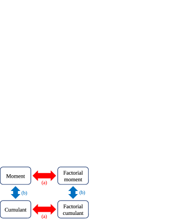
Figure 1: Relation between moments, cumulants, factorial moments, and factorial cumulants. The relations between moments and factorial moments are equivalent to those between cumulants and factorial cumulants (arrows (a)). Also, the relations between moments and cumulants are equivalent to those between factorial moments and factorial cumulants (arrows (b)).

As we have seen above, one of the sets of quantities, moments, cumulants and their factorials, can be represented by other quantities, and each set carries the same information on $P(n)$. From the above construction, it is clear that the relations between moments and factorial moments are the same as that between cumulants and factorial cumulants (arrows (a) in Fig. 1). Also, the relations between moments and cumulants are the same as that between factorial moments and factorial cumulants (arrows (b) in Fig. 1). These correspondences also hold for the multi-variable case discussed in the next section.

The factorial cumulants of Poisson distribution vanish except for the first order, i.e.

$$\langle n^{m}\rangle_{\rm fc,Poisson}=0\quad\mbox{(for $m\geq 2$)}.$$ (15)

This can be shown from the fact that the factorial-cumulant generating function of Poisson distribution is given by $K_{\rm Poisson}(s)=\lambda(s-1)$ Asakawa:2015ybt , with $\lambda=\langle n\rangle$ denoting the average. This property is useful to see the difference of a distribution from Poissonian one.

For a probability distribution function $P(x)$ for a continuous stochastic variable $x$, by defining the moment generating function as

$$G(\theta)=\int dxe^{\theta x}P(x),$$ (16)

all sets of quantities can be constructed in a similar manner.

II.2 Multi-variable case

Next, we consider the probability distribution function

$$P(n_{1},n_{2},\cdots,n_{M})=P(\bm{n})$$ (17)

for $M$ integer stochastic variables $\bm{n}=(n_{1},\cdots,n_{M})$, and its moments, cumulants, and their factorials. We consider these quantities for the linear combination of the stochastic variables given by

$$q_{(\bm{a})}=\sum_{i=1}^{M}a_{i}n_{i},$$ (18)

with $\bm{a}=(a_{1},\cdots,a_{M})$. Note that the conserved charges in heavy-ion collisions are given by the form in Eq. (18), where $n_{i}$ correspond to the particle numbers of various hadrons. For example, the net-baryon number $N_{\rm B}^{\rm(net)}$ is given by the baryon and anti-baryon numbers, $N_{\rm B}$ and $N_{\rm\bar{B}}$, as $N_{\rm B}^{\rm(net)}=N_{\rm B}-N_{\rm\bar{B}}$.

The $m$th order moment of $q_{(\bm{a})}$ is given by

$$\langle q_{(\bm{a})}^{m}\rangle=\sum_{\bm{n}}q_{(\bm{a})}^{m}P(\bm{n})=\sum_{\bm{n}}\Big{(}\sum_{i=1}^{M}a_{i}n_{i}\Big{)}^{m}P(\bm{n}),$$ (19)

where $\sum_{\bm{n}}$ denotes the sum over $n_{1},\cdots,n_{M}$. By defining the moment generating function as

$$G(\bm{\theta})=\sum_{\bm{n}}\Big{[}\prod_{i=1}^{M}e^{n_{i}\theta_{i}}\Big{]}P(\bm{n})=\Big{\langle}\prod_{i=1}^{M}e^{n_{i}\theta_{i}}\Big{\rangle},$$ (20)

with $\bm{\theta}=(\theta_{1},\cdots,\theta_{M})$, the moments of $q_{(\bm{a})}$ are given by

$$\langle q_{(\bm{a})}^{m}\rangle=\partial_{(\bm{a})}^{m}G(\bm{\theta})|_{\bm{\theta}=0}.$$ (21)

with

$$\partial_{(\bm{a})}=\sum_{i=1}^{M}a_{i}\frac{\partial}{\partial\theta_{i}}.$$ (22)

By introducing another linear combinations of $n_{i}$, $q_{(\bm{b})}=\sum_{i=1}^{M}b_{i}n_{i}$ and $q_{(\bm{c})}=\sum_{i=1}^{M}c_{i}n_{i}$, the mixed moment of $q_{(\bm{a})}$, $q_{(\bm{b})}$ and $q_{(\bm{c})}$, for example, is given by

$$\langle q_{(\bm{a})}q_{(\bm{b})}q_{(\bm{c})}\rangle =\sum_{\bm{n}}q_{(\bm{a})}q_{(\bm{b})}q_{(\bm{c})}P(\bm{n})$$

$$=\partial_{(\bm{a})}\partial_{(\bm{b})}\partial_{(\bm{c})}G(\bm{\theta})|_{\bm{\theta}=0}.$$ (23)

Next, the cumulants for $P(\bm{n})$ are defined from the cumulant generating function

$$K(\bm{\theta})=\ln G(\bm{\theta}),$$ (24)

as

$$\langle q_{(\bm{a})}^{m}\rangle_{\rm c}= \partial_{(\bm{a})}^{m}K(\bm{\theta})|_{\bm{\theta}=0},$$ (25)

$$\langle q_{(\bm{a})}q_{(\bm{b})}q_{(\bm{c})}\rangle_{\rm c}= \partial_{(\bm{a})}\partial_{(\bm{b})}\partial_{(\bm{c})}K(\bm{\theta})|_{\bm{\theta}=0},$$ (26)

and so forth.

The cumulants of $q_{(\bm{a})}$ are represented by moments as

$$\langle q_{(\bm{a})}\rangle_{\rm c}= \partial_{(\bm{a})}K=\partial_{(\bm{a})}\ln G=\frac{\partial_{(\bm{a})}G}{G}=\langle q_{(\bm{a})}\rangle,$$ (27)

$$\langle q_{(\bm{a})}^{2}\rangle_{\rm c}= \frac{\partial_{(\bm{a})}^{2}G}{G}-\frac{(\partial_{(\bm{a})}G)^{2}}{G^{2}}=\langle q_{(\bm{a})}^{2}\rangle-\langle q_{(\bm{a})}\rangle^{2}$$

$$= \langle(\delta q_{(\bm{a})})^{2}\rangle,$$ (28)

and so forth. One finds that these derivations are the same as the single variable case in Eqs. (6) – (8) with replacements of $n$ and $\partial_{\theta}$ in favor of $q_{(\bm{a})}$ and $\partial_{(\bm{a})}$. This means that $\langle q_{(\bm{a})}^{m}\rangle_{\rm c}$ can be interpreted as the cumulants of $q_{(\bm{a})}$ as if $q_{(\bm{a})}$ is a primary stochastic variable. This property of cumulants makes their interpretation clear, and enables us their practical calculation straightforward. As we will see below, this simple property does not hold for factorial moments and factorial cumulants, i.e. in general

$$\langle q_{(\bm{a})}^{m}\rangle_{\rm fc}\neq\langle q_{(\bm{a})}(q_{(\bm{a})}-1)\cdots(q_{(\bm{a})}-m+1)\rangle_{\rm c}.$$ (29)

The mixed cumulants are represented by moments with similar manipulations as in the previous section, for example,

$$\langle q_{(\bm{a})}q_{(\bm{b})}\rangle_{\rm c} =\partial_{(\bm{a})}\partial_{(\bm{b})}K=\frac{\partial_{(\bm{a})}\partial_{(\bm{b})}G}{G}-\frac{(\partial_{(\bm{a})}G)(\partial_{(\bm{b})}G)}{G^{2}}$$

$$=\langle q_{(\bm{a})}q_{(\bm{b})}\rangle-\langle q_{(\bm{a})}\rangle\langle q_{(\bm{b})}\rangle=\langle(\delta q_{(\bm{a})})(\delta q_{(\bm{b})})\rangle.$$ (30)

Next, we introduce factorial moments and factorial cumulants of $q_{(\bm{a})}$. We define these quantities from the generating functions

$$G_{\rm f}(\bm{s})= \sum_{\bm{n}}\Big{[}\prod_{i=1}^{M}s_{i}^{n_{i}}\Big{]}P(\bm{n})=\Big{\langle}\prod_{i=1}^{M}s_{i}^{n_{i}}\Big{\rangle},$$

$$K_{\rm f}(\bm{s})= \ln G_{\rm f}(\bm{s}),$$ (31)

with $\bm{s}=(s_{1},\cdots,s_{M})$ as

$$\langle q_{(\bm{a})}^{m}\rangle_{\rm f}=\bar{\partial}_{(\bm{a})}^{m}G_{\rm f}(\bm{s})|_{\bm{s}=1},\quad\langle q_{(\bm{a})}^{m}\rangle_{\rm fc}=\bar{\partial}_{(\bm{a})}^{m}K_{\rm f}(\bm{s})|_{\bm{s}=1},$$ (32)

with

$$\bar{\partial}_{(\bm{a})}=\sum_{i=1}^{M}a_{i}\frac{\partial}{\partial s_{i}}.$$ (33)

The mixed factorials are also defined as in Eq. (23), for example,

$$\langle q_{(\bm{a})}q_{(\bm{b})}q_{(\bm{c})}\rangle_{\rm fc}=\bar{\partial}_{(\bm{a})}\bar{\partial}_{(\bm{b})}\bar{\partial}_{(\bm{c})}K_{\rm f}(\bm{s})|_{\bm{s}=1}.$$ (34)

From these definitions, it is clear that the relation between moments and factorial moments is the same as that between cumulants and factorial cumulants (the arrows (a) in Fig. 1). The equivalence of the arrows (b) in Fig. 1 for the multi-variable case is also easily confirmed.

II.3 Relations between cumulants and factorial cumulants

Next, we relate cumulants and factorial cumulants for the multi-variable case. Although we concentrate on the relations between cumulants and factorial cumulants, the following results are applicable to those between moments and factorial moments.

Because the generating functions of cumulants and factorial cumulants, $K(\bm{\theta})$ and $K_{\rm f}(\bm{s})$, are related with each other by the change of variables $s_{i}=e^{\theta_{i}}$, their relations are obtained by rewriting $\bar{\partial}_{(\bm{a})}$ in terms of $\partial_{(\bm{a})}$. For the first order we have

$$\bar{\partial}_{(\bm{a})}=\sum_{i=1}^{M}a_{i}\frac{\partial}{\partial s_{i}}=\sum_{i=1}^{M}a_{i}\frac{\partial\theta_{i}}{\partial s_{i}}\frac{\partial}{\partial\theta_{i}}=\sum_{i=1}^{M}a_{i}\frac{1}{s_{i}}\frac{\partial}{\partial\theta_{i}},$$ (35)

where we used $\partial\theta_{i}/\partial s_{j}=0$ for $i\neq j$. By substituting $\bm{s}=1$, one obtains

$$\bar{\partial}_{(\bm{a})}=\partial_{(\bm{a})}.$$ (36)

The second derivative is calculated to be

$$\bar{\partial}_{(\bm{a})}\bar{\partial}_{(\bm{b})} =\sum_{i=1}^{M}a_{i}\frac{\partial}{\partial s_{i}}\sum_{j=1}^{M}b_{j}\frac{\partial}{\partial s_{j}}=\sum_{i,j=1}^{M}a_{i}\frac{\partial}{\partial s_{i}}b_{j}\frac{1}{s_{j}}\frac{\partial}{\partial\theta_{j}}$$

$$=\sum_{i,j=1}^{M}a_{i}b_{j}\left(-\frac{\delta_{ij}}{s_{j}^{2}}\frac{\partial}{\partial\theta_{j}}+\frac{1}{s_{i}s_{j}}\frac{\partial^{2}}{\partial\theta_{i}\partial\theta_{j}}\right).$$ (37)

Substituting $\bm{s}=1$, we have

$$\bar{\partial}_{(\bm{a})}\bar{\partial}_{(\bm{b})}=\partial_{(\bm{a})}\partial_{(\bm{b})}-\partial_{(\bm{ab})},$$ (38)

where we introduced the symbols

$$\partial_{(\bm{ab})} =\sum_{i=1}^{N}a_{i}b_{i}\frac{\partial}{\partial\theta_{i}},\quad\partial_{(\bm{abc})}=\sum_{i=1}^{N}a_{i}b_{i}c_{i}\frac{\partial}{\partial\theta_{i}},$$ (39)

$$\bar{\partial}_{(\bm{ab})} =\sum_{i=1}^{N}a_{i}b_{i}\frac{\partial}{\partial s_{i}},\quad\bar{\partial}_{(\bm{abc})}=\sum_{i=1}^{N}a_{i}b_{i}c_{i}\frac{\partial}{\partial s_{i}},$$ (40)

and so forth. Similar manipulations for higher orders lead to

$$\bar{\partial}_{(\bm{a})}\bar{\partial}_{(\bm{b})}\bar{\partial}_{(\bm{c})}= \partial_{(\bm{a})}\partial_{(\bm{b})}\partial_{(\bm{c})}-\left[\partial_{(\bm{a})}\partial_{(\bm{bc})}+({\rm 3~{}comb.})\right]+2\partial_{(\bm{abc})},$$ (41)

$$\bar{\partial}_{(\bm{a})}\bar{\partial}_{(\bm{b})}\bar{\partial}_{(\bm{c})}\bar{\partial}_{(\bm{d})}= \partial_{(\bm{a})}\partial_{(\bm{b})}\partial_{(\bm{c})}\partial_{(\bm{d})}-\left[\partial_{(\bm{a})}\partial_{(\bm{b})}\partial_{(\bm{cd})}+({\rm 6~{}comb.})\right]$$

$$+2\left[\partial_{(\bm{a})}\partial_{(\bm{bcd})}+({\rm 4~{}comb.})\right]+\left[\partial_{(\bm{ab})}\partial_{(\bm{cd})}+({\rm 3~{}comb.})\right]-6\partial_{(\bm{abcd})},$$ (42)

where “comb.” represents terms given by all possible combinations of subscripts, for example,

$$\partial_{(\bm{a})}\partial_{(\bm{bc})}+({\rm 3~{}comb.})=\partial_{(\bm{a})}\partial_{(\bm{bc})}+\partial_{(\bm{b})}\partial_{(\bm{ca})}+\partial_{(\bm{c})}\partial_{(\bm{ab})},$$ (43)

with the number denoting total number of the combinations.

Applying these derivatives to the generating functions and substituting $\bm{s}=1$, the factorial cumulants are translated into cumulants as

$$\langle q_{(\bm{a})}\rangle_{\rm fc} =\langle q_{(\bm{a})}\rangle_{\rm c},$$ (44)

$$\langle q_{(\bm{a})}q_{(\bm{b})}\rangle_{\rm fc} =\langle q_{(\bm{a})}q_{(\bm{b})}\rangle_{\rm c}-\langle q_{(\bm{ab})}\rangle_{\rm c},$$ (45)

$$\langle q_{(\bm{a})}q_{(\bm{b})}q_{(\bm{c})}\rangle_{\rm fc} =\langle q_{(\bm{a})}q_{(\bm{b})}q_{(\bm{b})}\rangle_{\rm c}$$

$$-\left[\langle q_{(\bm{a})}q_{(\bm{bc})}\rangle_{\rm c}+({\rm 3~{}comb.})\right]+2\langle q_{(\bm{abc})}\rangle_{\rm c},$$ (46)

and so forth. In particular, the factorial cumulants of $q_{(\bm{a})}$ are given by

$$\langle q_{(\bm{a})}^{2}\rangle_{\rm fc} =\langle q_{(\bm{a})}^{2}\rangle_{\rm c}-\langle q_{(\bm{a}^{2})}\rangle_{\rm c},$$ (47)

$$\langle q_{(\bm{a})}^{3}\rangle_{\rm fc} =\langle q_{(\bm{a})}^{3}\rangle_{\rm c}-3\langle q_{(\bm{a}^{2})}\rangle_{\rm c}+2\langle q_{(\bm{a}^{3})}\rangle_{\rm c},$$ (48)

where $q_{(\bm{a}^{2})}=q_{(\bm{aa})}$ and so forth. The relations up to sixth order are found in Ref. Nonaka:2017kko .

From the above results one can verify Eq. (29). In fact, Eq. (47) shows that $\langle q_{(\bm{a})}^{2}\rangle_{\rm fc}\neq\langle q_{(\bm{a})}(q_{(\bm{a})}-1)\rangle_{\rm c}$; only when all $a_{i}$ are $0$ or $1$, both sides in Eq. (29) are equivalent. This property of factorials make their interpretation and their calculation in practical analyses difficult; to calculate the factorial cumulants, one may construct them from cumulants using the relations (44)–(46).

It is also possible to represent cumulants by factorial cumulants. These relations are obtained by representing the $\bm{\theta}$ derivatives in terms of the $\bm{s}$ derivatives. Up to third order, we obtain

$$\langle q_{(\bm{a})}\rangle_{\rm c} =\langle q_{(\bm{a})}\rangle_{\rm fc}$$ (49)

$$\langle q_{(\bm{a})}q_{(\bm{b})}\rangle_{\rm c} =\langle q_{(\bm{a})}q_{(\bm{b})}\rangle_{\rm fc}+\langle q_{(\bm{ab})}\rangle_{\rm fc}$$ (50)

$$\langle q_{(\bm{a})}q_{(\bm{b})}q_{(\bm{c})}\rangle_{\rm c} =\langle q_{(\bm{a})}q_{(\bm{b})}q_{(\bm{b})}\rangle_{\rm fc}$$

$$+\left[\langle q_{(\bm{a})}q_{(\bm{bc})}\rangle_{\rm fc}+({\rm 3~{}comb.})\right]+\langle q_{(\bm{abc})}\rangle_{\rm fc}.$$ (51)

For the results up to sixth order, see Ref. Nonaka:2017kko .

II.4 Examples

In the previous subsection we obtained the factorial cumulants for linear combinations of stochastic variables $q_{(\bm{a})}$. To obtain the factorial cumulant of $n_{i}$ for a given $i$, we set the vector $\bm{a}$ so that $a_{i}=1$ while all other components are zero, which results in $q_{(\bm{a})}=n_{i}$. The factorial cumulants $\langle n_{i}^{m}\rangle_{\rm fc}$ are then represented by cumulants as

$$\langle n_{i}^{m}\rangle_{\rm fc}=\langle n_{i}(n_{i}-1)\cdots(n_{i}-m+1)\rangle_{\rm c},$$ (52)

which is the same result as Eq. (13). Similarly, the mixed factorial cumulant of two variables, for example, $\langle n_{1}^{m_{1}}n_{2}^{m_{2}}\rangle_{\rm fc}$, is obtained by substituting $\bm{a}=(1,0,\cdots,0)$ and $\bm{b}=(0,1,0,\cdots,0)$ into $\langle q_{(\bm{a})}^{m_{1}}q_{(\bm{b})}^{m_{2}}\rangle_{\rm fc}$ as

$$\langle n_{1}^{m_{1}}n_{2}^{m_{2}}\rangle_{\rm fc}= \langle q_{(\bm{a})}^{m_{1}}q_{(\bm{b})}^{m_{2}}\rangle_{\rm fc}$$

$$= \langle n_{1}(n_{1}-1)\cdots(n_{1}-m_{1}+1)$$

$$\times n_{2}(n_{2}-1)\cdots(n_{2}-m_{2}+1)\rangle_{\rm c},$$ (53)

where we used $q_{(\bm{a}^{m})}=q_{(\bm{a})}$, $q_{(\bm{b}^{m})}=q_{(\bm{b})}$, and $q_{(\bm{a}^{m_{1}}\bm{b}^{m_{2}})}=0$. The mixed factorial cumulants including more than two stochastic variables can also be obtained in a similar manner.

The operation of cumulant is compatible with the sum and multiplications of constant numbers; for example,

$$\langle(a_{1}n_{1}+a_{2}n_{2})^{2}\rangle_{\rm c}=a_{1}^{2}\langle n_{1}^{2}\rangle_{\rm c}+2a_{1}a_{2}\langle n_{1}n_{2}\rangle_{\rm c}+a_{2}^{2}\langle n_{2}^{2}\rangle_{\rm c},$$ (54)

which is clear from the definition in Eq. (25). This property also holds for factorial moments and factorial cumulants.

In relativistic field theory, conserved charges are given by the net number, i.e. the difference between particle and anti-particle numbers, $N_{\rm(net)}=N-\bar{N}$, with $N$ and $\bar{N}$ being particle and anti-particle numbers. The factorial cumulants of $N_{\rm(net)}$ are given by substituting $M=2$ and $a_{1,2}=\pm 1$, where $n_{1}$ and $n_{2}$ corresponds to $N$ and $\bar{N}$. The factorial cumulants of $N_{\rm(net)}$ are then calculated to be

$$\langle N_{\rm(net)}\rangle_{\rm fc} =\langle N_{\rm(net)}\rangle_{\rm c},$$ (55)

$$\langle N_{\rm(net)}^{2}\rangle_{\rm fc} =\langle N_{\rm(net)}^{2}\rangle_{\rm c}-\langle N_{\rm(tot)}\rangle_{\rm c},$$ (56)

$$\langle N_{\rm(net)}^{3}\rangle_{\rm fc} =\langle N_{\rm(net)}^{3}\rangle_{\rm c}-3\langle N_{\rm(net)}N_{\rm(tot)}\rangle_{\rm c},+2\langle N_{\rm(net)}\rangle_{\rm c},$$ (57)

and so forth, where $N_{\rm(tot)}=N+\bar{N}$ is the total particle number. These results show that the factorial cumulants of $N_{\rm(net)}$ cannot be written solely by the cumulants of $N_{\rm(net)}$, but contain those of $N_{\rm(tot)}$.

As discussed in Sec. II.1, the factorial cumulants of Poisson distribution vanishes except for the first order as in Eq. (15). This property also holds for the multi-variable case. When the distributions of $n_{1},\cdots,n_{M}$ obey Poissonian independently, i.e. $P(\bm{n})=\prod_{i}P_{\rm Poisson}(n_{i})$, we have

$$\langle q_{(\bm{a})}^{m}\rangle_{\rm fc,Poisson}=0\quad\mbox{(for $m\geq 2$)}.$$ (58)

This can be shown from the fact that the factorial-cumulant generating function in this case is linear in $\bm{s}$.

II.5 Factorials of continuous functions

Next we consider the moments, cumulants, and their factorials of continuous functions. We consider a probability distribution functional $P[\rho(x)]$ of a one-dimensional function $\rho(x)$. The moment generating function in this case is defined by

$$G[\theta(x)]=\int{\cal D}\rho e^{\int dx\theta(x)\rho(x)}P[\rho(x)],$$ (59)

where $\int{\cal D}\rho$ represents the functional integral, which satisfies $\int{\cal D}\rho P[\rho(x)]=1$. The moments of $\rho(x)$ are then given by the functional derivatives of $G[\theta(x)]$ as

$$\langle\rho(x_{1})\rho(x_{2})\cdots\rho(x_{l})\rangle= \int{\cal D}\rho\rho(x_{1})\cdots\rho(x_{l})P[\rho(x)]$$

$$= \frac{\delta}{\delta\theta(x_{1})}\cdots\frac{\delta}{\delta\theta(x_{l})}G[\theta(x)]|_{\theta(x)=0}.$$ (60)

The cumulants, factorial moments and factorial cumulants are defined similarly from functional derivatives with respect to $\theta(x)$ or $s(x)$ of the generating functions

$$G_{\rm f}[s(x)] =\int{\cal D}\rho e^{\int dx\rho(x)\ln s(x)}P[\rho(x)],$$ (61)

$$K[\theta(x)] =\ln G[\theta(x)],\quad K_{\rm f}[s(x)]=\ln G_{\rm f}[s(x)],$$ (62)

respectively.

The relation between moments and factorial moments in this case is obtained from functional derivatives as

$$\langle\rho(x_{1})\rangle= \frac{\delta}{\delta\theta(x_{1})}G=\frac{\delta s(x_{1})}{\delta\theta(x_{1})}\frac{\delta}{\delta s(x_{1})}G_{\rm f}=\langle\rho(x_{1})\rangle_{\rm f},$$ (63)

$$\langle\rho(x_{1})\rho(x_{2})\rangle= \frac{\delta^{2}G}{\delta\theta(x_{1})\delta\theta(x_{2})}=\frac{\delta s(x_{1})}{\delta\theta(x_{1})}\frac{\delta s(x_{2})}{\delta\theta(x_{2})}\frac{\delta^{2}G_{\rm f}}{\delta s(x_{1})\delta s(x_{2})}+\frac{\delta^{2}s(x_{1})}{\delta\theta(x_{1})\delta\theta(x_{2})}\frac{\delta G_{\rm f}}{\delta s(x_{1})}$$

$$= \langle\rho(x_{1})\rho(x_{2})\rangle_{\rm f}+\delta(x_{1}-x_{2})\langle\rho(x_{1})\rangle_{\rm f},$$ (64)

$$\langle\rho(x_{1})\rho(x_{2})\rho(x_{3})\rangle= \langle\rho(x_{1})\rho(x_{2})\rho(x_{3})\rangle_{\rm f}$$

$$+\delta(x_{1}-x_{2})\langle\rho(x_{1})\rho(x_{3})\rangle_{\rm f}+\delta(x_{2}-x_{3})\langle\rho(x_{2})\rho(x_{1})\rangle_{\rm f}+\delta(x_{3}-x_{1})\langle\rho(x_{3})\rho(x_{2})\rangle_{\rm f}$$

$$+\delta(x_{1}-x_{2})\delta(x_{1}-x_{3})\langle\rho(x_{1})\rangle_{\rm f},$$ (65)

where we used $\delta s(x_{1})/\delta\theta(x_{2})=\delta(x_{1}-x_{2})\partial s(x_{1})/\partial\theta(x_{1})$. The same manipulation can be repeated to arbitrary higher orders.

The moments $\langle\rho(x_{1})\cdots\rho(x_{m})\rangle$ and cumulants $\langle\rho(x_{1})\cdots\rho(x_{m})\rangle_{\rm c}$ are usually called correlation functions. In particular, the cumulants correspond to the “connected part” of the correlation function Asakawa:2015ybt , and play useful roles for various purposes. The meanings of their factorials, $\langle\rho(x_{1})\cdots\rho(x_{m})\rangle_{\rm f}$ and $\langle\rho(x_{1})\cdots\rho(x_{m})\rangle_{\rm fc}$, will be discussed in Secs. III.2 and III.3.

When $\rho(x)$ represents a charge density, the total charge in a finite interval $\Delta$ is given by the integral of $\rho(x)$ as

$$Q_{\Delta}=\int_{\Delta}dx\rho(x).$$ (66)

The cumulants of $Q_{\Delta}$ is given by

$$\langle Q_{\Delta}^{m}\rangle_{\rm c}= \int_{\Delta}dx_{1}\frac{\delta}{\delta\theta(x_{1})}\cdots\int_{\Delta}dx_{M}\frac{\delta}{\delta\theta(x_{m})}K[\theta(x)]|_{\theta(x)=0}$$

$$= \int_{\Delta}dx_{1}\cdots\int_{\Delta}dx_{M}\langle\rho(x_{1})\cdots\rho(x_{m})\rangle_{\rm c}.$$ (67)

Other quantities, moments and factorials, are also given similarly. From the construction it is clear that the moments, cumulants, and their factorials of $Q_{\Delta}$ satisfy the relations obtained in Sec. II.1.

III Properties of cumulants and factorial cumulants

In this section, we discuss properties of factorial moments and factorial cumulants which would be important in the study of fluctuations in relativistic heavy-ion collisions.

III.1 Thermal fluctuations

An important characteristics of the cumulants of conserved charges in a thermal system is that they are directly connected to grand partition function and are calculable in statistical mechanics, while the factorial cumulants generally do not have such a property. In a thermal system described by the grand partition function

$$Z={\rm Tr}e^{-\beta(H-\mu N)},$$ (68)

with Hamiltonian $H$, inverse temperature $\beta=1/T$, a conserved charge $N$ and its chemical potential $\mu$, the cumulants of $N$ are given by Asakawa:2015ybt

$$\langle N^{m}\rangle_{\rm c}=-\frac{\partial^{m}}{\partial(\beta\mu)^{m}}\ln Z.$$ (69)

Using this relation, $\langle N^{m}\rangle_{\rm c}$ are calculable in statistical mechanics without ambiguity. Equation (69) also suggests the relation between the cumulants

$$\langle N^{m+1}\rangle_{\rm c}=\frac{\partial}{\partial(\beta\mu)}\langle N^{m}\rangle_{\rm c},$$ (70)

which plays a quite useful role in understanding the sign of higher-order cumulants near the QCD critical point Asakawa:2009aj . These arguments are not applicable to the cumulants of non-conserved quantities, because they have no direct connection to the partition function like Eq. (69) Asakawa:2015ybt .

The factorial cumulants in general have no direct connection to the partition function, either. In fact, conserved charges in QCD are given by a net particle number $N_{\rm(net)}=N-\bar{N}$, and their factorial cumulants contain the total particle number $N_{\rm(tot)}$ when they are represented by cumulants as in Eqs. (55)–(57). Because the total particle number is not a conserved charge in QCD, the factorial cumulants have no direct connection to the partition function, and hence are not calculable unambiguously based on QCD and statistical mechanics. Similarly, the factorial cumulants of particle and anti-particle numbers $N$ and $\bar{N}$ cannot be represented by the cumulants of conserved charge $N_{\rm(net)}$. Only in extremely dense systems in which the anti-particle density is negligible, $N\gg\bar{N}$, we have $N_{\rm(net)}\simeq N_{\rm(tot)}\simeq N$ and the factorial cumulants of $N_{\rm(net)}$ can be constructed from conserved-charge cumulants.

Next, let us give a few remarks on the use of factorial cumulants in the search of QCD critical point. It is known that the cumulants of conserved charges diverge at the critical point. This divergence is more steeper for higher orders Stephanov:2008qz . This means that, in the very vicinity of the critical point, the cumulants satisfy

$$\langle N_{\rm(net)}\rangle_{\rm c}\ll\langle N_{\rm(net)}^{2}\rangle_{\rm c}\ll\langle N_{\rm(net)}^{3}\rangle_{\rm c}\ll\langle N_{\rm(net)}^{4}\rangle_{\rm c}.$$ (71)

When Eq. (71) is satisfied, the cumulants and factorial cumulants can be regarded identical Ling:2015yau , because the factorial cumulants are given by the linear combination of the cumulants with a common highest-order term. We, however, emphasize that the experimental results by STAR and ALICE collaborations Adamczyk:2013dal ; Adamczyk:2014fia ; Thader:2016gpa ; ALICE:QM17 show that the idealization like Eq. (71) is not applicable to the results on higher order cumulants. Therefore, in the study of these experimental results cumulants and factorial cumulants have to be distinguished.

III.2 Factorials and correlation functions

Next, we consider a system composed of classical particles carrying a charge, and show that the factorial moments and factorial cumulants of the total charge in a spatial volume, respectively, corresponds to the moments and cumulants after removing the trivial correlations of individual particles Ling:2015yau ; Bzdak:2016sxg .

Let us consider a classical one-dimensional system composed of particles having a unit charge. The charge density $\rho(x)$ of this system is given by

$$\rho(x)=\sum_{i=1}^{I}\delta(x-z_{i}),$$ (72)

where $I$ is the total particle number in the system and $z_{i}$ are the positions of particles.

From Eq. (72) and the property of delta function $\delta(x-y)\delta(y-z)=\delta(x-z)\delta(y-z)$, the products of $\rho(x)$ are rewritten as

$$\rho(x_{1})\rho(x_{2})= \sum_{i,j}\delta(x_{1}-z_{i})\delta(x_{2}-z_{j})$$

$$= \sum_{i\neq j}\delta(x_{1}-z_{i})\delta(x_{2}-z_{j})$$

$$+\delta(x_{1}-x_{2})\sum_{i}\delta(x_{1}-z_{i}),$$ (73)

$$\rho(x_{1})\rho(x_{2})\rho(x_{3})= \sum_{i,j,k}\delta(x_{1}-z_{i})\delta(x_{2}-z_{j})\delta(x_{3}-z_{k})$$

$$= \sum_{i\neq j,j\neq k,k\neq i}\delta(x_{1}-z_{i})\delta(x_{2}-z_{j})\delta(x_{3}-z_{k})$$

$$+\delta(x_{1}-x_{2})\sum_{i\neq k}\delta(x_{1}-z_{i})\delta(x_{3}-z_{k})$$

$$+\delta(x_{2}-x_{3})\sum_{j\neq i}\delta(x_{2}-z_{j})\delta(x_{1}-z_{i})$$

$$+\delta(x_{3}-x_{1})\sum_{k\neq j}\delta(x_{3}-z_{k})\delta(x_{2}-z_{j})$$

$$+\delta(x_{1}-x_{2})\delta(x_{1}-x_{3})\sum_{i}\delta(x_{1}-z_{i}),$$ (74)

and so forth. By taking the expectation values of both sides and comparing them with Eqs. (63)–(65), one finds that the factorial moments of $\rho(x)$ are given by the corresponding moments but without the contribution of the self correlation,

$$\langle\rho(x_{1})\rho(x_{2})\cdots\rho(x_{m})\rangle_{\rm f}$$

$$=\sum_{\begin{subarray}{c}i_{1},\cdots,i_{m}\\ i_{l}\neq i_{k}\\ (l,k=1,\cdots,m)\end{subarray}}\langle\delta(x_{1}-z_{i_{1}})\delta(x_{2}-z_{i_{2}})\cdots\delta(x_{m}-z_{i_{m}})\rangle.$$ (75)

The factorial moments $\langle Q_{\Delta}^{m}\rangle_{\rm f}$ of a charge in an interval $\Delta$ in Eq. (66) are also understood as the moments of $Q_{\Delta}$ but without the self correlation. Since factorial cumulants are constructed from the factorial moments with the same relation between cumulants and moments as in Fig. 1, they are interpreted as the cumulants without the self correlation, too. This interpretation for factorial moments and factorial cumulants is valid for arbitrary higher orders.

The same conclusion is obtained for a system composed of multi-particle species having non-unit charges. In this case, the density of a charge is given by

$$\rho(x)= \sum_{t}e_{t}\rho_{t}(x)$$ (76)

with

$$\rho_{t}(x)= \sum_{i=1}^{I_{t}}\delta(x-z_{i}),$$ (77)

where $e_{t}$ is the charge carried by particles labeled by $t$ with the total number $I_{t}$, and the sum for $t$ runs over all particle species. The probability density functional is extended to those of the densities, $P[\rho_{1}(x),\rho_{2}(x),\cdots]$. By defining the factorial generating functionals for $P[\rho_{1}(x),\rho_{2}(x),\cdots]$ and repeating the same calculation, it is possible to conclude that the factorial moments and factorial cumulants of Eq. (76) can be understood as the moments and cumulants without the self correlation even in this case.

We note that the above property of factorials is applicable only to classical systems in which the density is given in the form (76). In such systems, factorials would play a useful role in studying correlations between different particles Bzdak:2016sxg . In a system in which the classical particle picture is not applicable, however, this argument is no longer applicable. Because the system near the QCD critical point would belong to the latter case, one has to keep this limitation in mind when the factorial cumulants are applied to the search of the critical point.

III.3 Hadronization and resonance decays

In relativistic heavy-ion collisions, degrees of freedom carrying charges change during the time evolution. In the deconfined medium in the early stage, charges are carried by quarks. These degrees of freedom are confined into hadrons at hadronization. Even after the hadronization and chemical freezeout, particle species continue to change by the inelastic scatterings and resonance formations. In this subsection, we consider the meaning of factorial cumulants in systems in which particle species change by these reactions.

For this purpose, let us consider a simple model composed of doubly charged particles in some unit, whose particle number $N$ is distributed by the probability distribution function $P(N)$. Then, we suppose that all particles decay into two particles having a unit charge, respectively. The number $n$ of decayed particles is then given by $n=2N$, and thus the probability distribution function of $n$ is given by

$$\tilde{P}(n)=\sum_{N}\delta_{n,2N}P(N).$$ (78)

In the following we calculate the cumulants and factorial cumulants before and after the decay, and show that factorial cumulants change their values by this reaction, while the values of cumulants are conserved.

Let us first consider the moments. The moment generating function of $\tilde{P}(n)$ is given by

$$\tilde{G}(\theta) =\sum_{n}e^{n\theta}\tilde{P}(n)=\sum_{n,N}e^{n\theta}\delta_{n,2N}P(N)$$

$$=\sum_{N}e^{2N\theta}P(N)=G(2\theta),$$ (79)

where $G(\theta)=\sum_{N}e^{N\theta}P(N)$ is the moment generating function of $P(N)$. The moments of $n$ are obtained by taking $\theta$ derivative of Eq. (79). From Eq. (79), we obtain $\partial_{\theta}^{m}\tilde{G}=(2\partial_{\theta})^{m}G$ for $\theta=0$, which gives

$$\langle n^{m}\rangle=\langle(2N)^{m}\rangle,$$ (80)

where the expectation values of the left- and right-hand sides are taken for $\tilde{P}(n)$ and $P(N)$, respectively. Equation (80) is reasonable in the light of charge conservation; because the total charge does not change by the decay, its moments are not altered. Similarly, one can show the same conclusion for cumulants, i.e. $\langle n^{m}\rangle_{\rm c}=\langle(2N)^{m}\rangle_{\rm c}$.

Next let us consider the factorial moments. The factorial-moment generating function of $\tilde{P}(n)$ is calculated to be

$$\tilde{G}_{\rm f}(s)=\sum_{n}s^{n}\tilde{P}(n)=\sum_{N}s^{2N}P(N)=G_{\rm f}(s^{2}),$$ (81)

with $G_{\rm f}(\theta)=\sum_{N}s^{N}P(N)$. By taking the $s$ derivatives of Eq. (81) and substituting $s=1$ one finds,

$$\langle n\rangle_{\rm f} =\langle 2N\rangle_{\rm f},\quad\langle n^{2}\rangle_{\rm f}=\langle(2N)^{2}\rangle_{\rm f}+\langle 2N\rangle_{\rm f},$$

$$\langle n^{3}\rangle_{\rm f} =\langle(2N)^{3}\rangle_{\rm f}+3\langle(2N)^{2}\rangle_{\rm f},$$ (82)

and so forth. This result shows that the factorial moments change their values by the decay contrary to the case of moments in Eq. (80) except for the first order. The same conclusion holds for factorial cumulants, i.e. $\langle n^{m}\rangle_{\rm fc}\neq\langle(2N)^{m}\rangle_{\rm fc}$.

Because the values of factorial cumulants (moments) are not conserved by reactions changing particle species as in this example, their values are sensitive to the reactions. In relativistic heavy-ion collisions, particle species carrying charges continue to change by hadronization around the phase boundary and by inelastic scatterings until the final state. The factorial cumulants would be altered in non-trivial ways by these processes. When one applies factorial cumulants in the analysis of fluctuations in heavy-ion collisions, this property has to be remembered.

IV Factorial cumulants in the binomial model

From the discussion in the previous section, it seems that in relativistic heavy-ion collisions factorial cumulants do not have clear advantages compared to cumulants. Nevertheless, in the rest of this paper we discuss that the factorial cumulants can play quite useful roles for some purposes in the study of fluctuations. We pick up three such examples in Secs. V, VI, and VII. All of them are to some extent related to the reconstruction of the “original” fluctuations from the experimental data obtained in constrained and/or incomplete conditions.

All of these applications are related to the binomial model Kitazawa:2011wh ; Kitazawa:2012at ; Bzdak:2012ab ; Bzdak:2013pha ; Luo:2014rea ; Asakawa:2015ybt ; Kitazawa:2016awu ; Nonaka:2017kko . In this section, therefore, we first give a brief review on the binomial model, and derive relations between the factorial cumulants in this model, which play a central role in the subsequent sections.

IV.1 The binomial model

For an illustration of the binomial model Asakawa:2015ybt , let us consider a probability distribution function $P(N)$ for an integer stochastic variable $N$. We suppose that $N$ is the number of particles in each “event”, and we are interested in the cumulants of the event-by-event fluctuation of $N$. We further suppose that the particle number in each event is counted by a detector. However, the detector cannot measure the particles definitely, but only with a probability $p$ less than unity. The probability $p$ is called efficiency. Then, the distribution of the particle number $n$ observed by the detector in each event, $\tilde{P}(n)$, and accordingly its cumulants, is different from those of the actual number $N$. The problem considered here is to obtain the cumulants of $P(N)$ from the information on $\tilde{P}(n)$ obtained in this incomplete experiment.

This problem can be resolved completely when the probabilities to observe particles are uncorrelated for individual particles. Then, if the actual particle number in an event is $N$, the probability to observe $n$ particles in this event is given by the binomial distribution function

$$B_{p,N}(n)={{}_{N}C_{n}}p^{n}(1-p)^{N-n},$$ (83)

where ${}_{N}C_{n}=\frac{N!}{n!(N-n)!}$ is the binomial coefficient. The distribution function $\tilde{P}(n)$ thus is related to $P(N)$ as

$$\tilde{P}(n)=\sum_{N}B_{p,N}(n)P(N).$$ (84)

We refer to Eq. (84) as the binomial model. This model was employed to connect baryon and proton number cumulants Kitazawa:2011wh ; Kitazawa:2012at and for the efficiency correction Kitazawa:2012at ; Bzdak:2012ab . We will see in the next section how to perform the efficiency correction in the binomial model.

The binomial model (84) can be extended to multi-variable systems. Suppose a system composed of $M$ particle species, and that the probability that particle numbers $N_{1},\ N_{2},\cdots,N_{M}$ are obtained in an “event” is given by the probability distribution function $P(N_{1},\ N_{2},\cdots,N_{M})=P(\bm{N})$. We also assume that the particles labeled by $i$ are measured with an efficiency $p_{i}$. We denote the observed particle numbers as $n_{i}$, and the probability distribution function of $n_{i}$ as $\tilde{P}(\bm{n})$. Assuming the independence of the efficiencies for individual particles, the distribution functions $P(\bm{N})$ and $\tilde{P}(\bm{n})$ are related with each other as

$$\tilde{P}(\bm{n})=\sum_{\bm{N}}P(\bm{N})\prod_{i=1}^{M}B_{p_{i},N_{i}}(n_{i}).$$ (85)

IV.2 Factorial cumulants in binomial model

Next, we relate the factorial cumulants of $\tilde{P}(\bm{n})$ and $P(\bm{N})$ in the binomial model (85). To obtain these relations, it is convenient to use the generating functions of $\tilde{P}(\bm{n})$ and $P(\bm{N})$. First, the factorial-moment generating function of the binomial distribution (83) is given by

$$G_{{\rm f};p,N}^{\rm(binomial)}(s)=\sum_{n}B_{p,N}(n)s^{n}=(1+p(s-1))^{N}.$$ (86)

Using Eq. (86), the factorial-moment generating function of $\tilde{P}(\bm{n})$ is calculated to be,

$$\tilde{G}_{\rm f}(\bm{s}) =\sum_{\bm{n}}\tilde{P}(\bm{n})\prod_{i=1}^{M}s_{i}^{n_{i}}$$

$$=\sum_{\bm{N}}P(\bm{N})\sum_{\bm{n}}\prod_{i=1}^{M}B_{p_{i},N_{i}}(n_{i})s_{i}^{n_{i}}$$

$$=\sum_{\bm{N}}P(\bm{N})\prod_{i=1}^{M}(1+p_{i}(s_{i}-1))^{N_{i}}$$

$$=G_{\rm f}(\bm{s}^{\prime}),$$ (87)

with $s^{\prime}_{i}=1+p_{i}(s_{i}-1)$, and $G_{\rm f}(\bm{s})$ is the factorial-moment generating function of $P(\bm{N})$. The same relation holds between factorial-cumulant generating functions,

$$\tilde{K}_{\rm f}(\bm{s})=\ln\tilde{G}_{\rm f}(\bm{s})=\ln G_{\rm f}(\bm{s}^{\prime})=K_{\rm f}(\bm{s}^{\prime}).$$ (88)

From Eq. (87), one finds that $\bar{\partial}_{(\bm{a})}\tilde{K}_{\rm f}=\bar{\partial}_{(\bm{ap})}K_{\rm f}$ and

$$\bar{\partial}_{(\bm{a})}^{m}K_{\rm f}=\bar{\partial}_{(\bm{a}/\bm{p})}^{m}\tilde{K}_{\rm f},\quad\bar{\partial}_{(\bm{a})}\bar{\partial}_{(\bm{b})}K_{\rm f}=\bar{\partial}_{(\bm{a}/\bm{p})}\bar{\partial}_{(\bm{b}/\bm{p})}\tilde{K}_{\rm f},$$ (89)

and so forth, where it is understood that $\bm{s}=1$ is substituted and $\bar{\partial}_{(\bm{a}/\bm{p})}=\sum_{i=1}^{M}(a_{i}/p_{i})\partial_{s_{i}}$. Equation (89) shows that the factorial cumulants of $\tilde{P}(\bm{n})$ and $P(\bm{n})$ are connected by simple relations Nonaka:2017kko

$$\langle Q_{(\bm{a})}^{m}\rangle_{\rm fc}=\langle q_{(\bm{a}/\bm{p})}^{m}\rangle_{\rm fc},\quad\langle Q_{(\bm{a})}Q_{(\bm{b})}\rangle_{\rm fc}=\langle q_{(\bm{a}/\bm{p})}q_{(\bm{b}/\bm{p})}\rangle_{\rm fc},$$

$$\langle Q_{(\bm{a})}Q_{(\bm{b})}Q_{(\bm{c})}\rangle_{\rm fc}=\langle q_{(\bm{a}/\bm{p})}q_{(\bm{b}/\bm{p})}q_{(\bm{c}/\bm{p})}\rangle_{\rm fc},$$ (90)

and so forth, where we defined linear combinations of $N_{i}$ and $n_{i}$, respectively, as $Q_{(\bm{a})}=\sum_{i=1}^{M}a_{i}N_{i}$ and $q_{(\bm{a})}=\sum_{i=1}^{M}a_{i}n_{i}$. The expectation values of $Q_{(\bm{a})}$ and $q_{(\bm{a})}$ are taken for $P(\bm{n})$ and $\tilde{P}(\bm{n})$, respectively. Equation (90) is the important relation which play central roles in the subsequent sections.

We finally note that the same relations as in Eq. (90) hold for factorial moments, as one can easily show from Eq. (87). This property of factorial moments are used in Refs. Bzdak:2012ab ; Bzdak:2013pha ; Luo:2014rea for the efficiency correction of cumulants.

V Efficiency correction

In this section, as an example of a problem in which the relation (90) plays a useful role we first consider the problem of the efficiency correction of cumulants, i.e. the reconstruction of the original cumulants from observed ones, following Ref. Nonaka:2017kko .

In the efficiency correction, one has to represent the cumulants of the genuine particle number distribution $P(\bm{N})$ from those of the observed distribution $\tilde{P}(\bm{n})$ as discussed in Sec. IV.1. In the binomial model, these relations are obtained straightforwardly with the use of Eq. (90). In fact, the cumulants of $Q_{(\bm{a})}$ can be represented by those of $q_{(\bm{a})}$ by the following three steps:

1. Convert a cumulant of $P(\bm{N})$ into factorial cumulants.

2. Convert the factorial cumulants of $P(\bm{N})$ into factorial cumulants of $\tilde{P}(\bm{N})$ using Eq. (90).

3. Convert the factorial cumulants of $\tilde{P}(\bm{N})$ into cumulants.

As an example, we show the explicit manipulation for the second and third orders:

$$\langle Q_{(\bm{a})}^{2}\rangle_{\rm c}= \langle Q_{(\bm{a})}^{2}\rangle_{\rm fc}+\langle Q_{(\bm{a}^{2})}\rangle_{\rm fc}=\langle q_{(\bm{a}/\bm{p})}^{2}\rangle_{\rm fc}+\langle q_{(\bm{a}^{2}/\bm{p})}\rangle_{\rm fc}$$

$$= \langle q_{(\bm{a}/\bm{p})}^{2}\rangle_{\rm c}-\langle q_{(\bm{a}^{2}/\bm{p}^{2})}\rangle_{\rm c}+\langle q_{(\bm{a}^{2}/\bm{p})}\rangle_{\rm c},$$ (91)

$$\langle Q_{(\bm{a})}^{3}\rangle_{\rm c}= \langle Q_{(\bm{a})}^{3}\rangle_{\rm fc}+3\langle Q_{(\bm{a})}Q_{(\bm{a}^{2})}\rangle_{\rm fc}+\langle Q_{(\bm{a}^{3})}\rangle_{\rm fc}$$

$$= \langle q_{(\bm{a}/\bm{p})}^{3}\rangle_{\rm fc}+3\langle q_{(\bm{a}/\bm{p})}q_{(\bm{a^{2}/p})}\rangle_{\rm fc}+\langle q_{(\bm{a}^{3}/\bm{p})}\rangle_{\rm fc}$$

$$= \langle q_{(\bm{a}/\bm{p})}^{3}\rangle_{\rm c}-3\langle q_{(\bm{a}/\bm{p})}q_{(\bm{a^{2}/p^{2}})}\rangle_{\rm c}+2\langle q_{(\bm{a}^{3}/\bm{p}^{3})}\rangle_{\rm c}$$

$$+3\bigl{(}\langle q_{(\bm{a}/\bm{p})}q_{(\bm{a}^{2}/\bm{p})}\rangle_{\rm c}-\langle q_{(\bm{a}^{3}/\bm{p}^{2})}\rangle_{\rm c}\bigr{)}+\langle q_{(\bm{a}^{3}/\bm{p})}\rangle,$$ (92)

where three equalities in Eqs. (91) and (92) correspond to the three steps shown above. In Eqs. (91) and (92), the cumulants of genuine particle numbers $Q_{(\bm{a})}$ are represented by those of observed particle numbers. Because the latter cumulants are experimentally observable, one can construct genuine cumulants using these relations. The same manipulation is applicable to arbitrary higher orders. More detailed discussion, as well as the explicit results up to sixth order and mixed cumulants, is found in Ref. Nonaka:2017kko .

We note that the last steps in Eqs. (91) and (92), i.e. the conversion from factorial cumulants to cumulants, is necessary to carry out the numerical analysis effectively. This is because the calculation of the factorial cumulants is not as simple as cumulants because of Eq. (29). The above procedure of the efficiency correction can drastically reduce the numerical costs compared to those in Ref. Bzdak:2013pha ; Luo:2014rea when the order of the cumulant is large Nonaka:2017kko . This method also simplifies the analytic manipulation compared to the method proposed in Ref. Kitazawa:2016awu .

VI Dependence on momentum cuts

In this and next sections, we apply factorial cumulants to the analyses of the acceptance dependences of fluctuation observables, and show that they play unique roles in these analyses. In this section we first study the dependence on the momentum cuts.

The detectors for heavy-ion collisions can measure particles in a finite transverse-momentum ($p_{T}$) range. For example, the STAR detector Thader:2016gpa can measure protons and anti-protons in the range $0.4<p_{T}<0.8$ GeV using time projection chamber (TPC). The range can be extended to $0.4<p_{T}<2.0$ GeV with the simultaneous use of time of flight (TOF), although the efficiency is lowered for $p_{T}>0.8$ GeV. Although the maximum $p_{T}$ range is determined by the detector, the range can be varied by introducing $p_{T}$ cuts within the maximum coverage allowed by the detector. The dependence of the net-proton number cumulants on the $p_{T}$ range has been analyzed by the STAR collaboration Thader:2016gpa ; Luo:2017faz . These experimental analyses show that the cumulants have clear $p_{T}$-cut dependence.

To describe the $p_{T}$-cut dependences of the fluctuation observables, let us assume a simple model that particles are emitted to different $p_{T}$ independently. Then, the probability that a particle arrives at a given $p_{T}$ range is simply given by the ratio of the particle yield in the $p_{T}$ range and the total one. Moreover, the probabilities for individual particles are independent. In this case, therefore, the measurement of particles in the $p_{T}$ range is regarded as the same problem of the efficiency correction in the binomial model discussed in the previous section.

To be more specific, let us consider a system with $M$ particle species and denote the particle numbers in each event as $N_{1},\cdots,N_{M}$. When these particles are measured with a $p_{T}$ cut, $n_{1},\cdots,n_{M}$ particles among them are observed in the $p_{T}$ range. Assuming the independent particle emission, the relation between the particle numbers $N_{1},\cdots,N_{M}$ and $n_{1},\cdots,n_{M}$ are given by the binomial model Eq. (85). The probability to measure a particle labeled by $i$ in the $p_{T}$ range, which corresponds to the efficiency in the previous sections, is simply given by the ratio

$$p_{i}=\frac{\langle n_{i}\rangle}{\langle N_{i}\rangle}.$$ (93)

As discussed in Sec. IV, the factorial cumulants in the binomial model are related with each other through Eq. (90). Substituting $\bm{a}=(1,0,\cdots,0)$, $\bm{b}=(0,1,0,\cdots,0)$, and so forth into Eq. (90) one obtains

$$\langle n_{i_{1}}\cdots n_{i_{m}}\rangle_{\rm fc}=p_{i_{1}}\cdots p_{i_{m}}\langle N_{i_{1}}\cdots N_{i_{m}}\rangle_{\rm fc}.$$ (94)

Furthermore, using Eq. (93) we have

$$\frac{\langle n_{i_{1}}\cdots n_{i_{m}}\rangle_{\rm fc}}{\langle n_{i_{1}}\rangle\cdots\langle n_{i_{m}}\rangle}=\frac{\langle N_{i_{1}}\cdots N_{i_{m}}\rangle_{\rm fc}}{\langle N_{i_{1}}\rangle\cdots\langle N_{i_{m}}\rangle}.$$ (95)

The left-hand side of this equation is experimentally observable with various $p_{T}$ ranges, while the right-hand side is the genuine factorial cumulant with the full momentum acceptance. Because the right-hand side does not depend on the $p_{T}$ range, Eq. (95) tells us that the left-hand side does not have $p_{T}$ range dependence. Therefore, the assumption of the independent particle emission can be checked experimentally by plotting the left-hand side of Eq. (95); if this plot were constant as a function of $p_{T}$ range, it supports the independent particle emission. Moreover, in this case Eq. (95) can also be used to determine the right-hand side, i.e. the factorial cumulants with full momentum coverage $\langle N_{i_{1}}\cdots N_{i_{m}}\rangle_{\rm fc}$, by performing a constant fit to the data. In this way, one can obtain various factorial cumulants for full momentum coverage using Eq. (95). The factorial cumulants can then be used to analyze the genuine cumulants of conserved charges, which are quantities suitable for a comparison with theoretical analysis.

Note that the above procedure is similar to the efficiency correction discussed in Sec. V, but has two unique features. First, one can inspect the validity of the use of the binomial model using the experimental data for various $p_{T}$ cuts. Second, the simultaneous use of the experimental results obtained with various $p_{T}$ cuts should be responsible for reducing the statistical error of the reconstructed factorial cumulants.

It is also noteworthy that Eq. (95) shows that the factorial cumulants have a power-law behavior,

$$\langle n_{i_{1}}\cdots n_{i_{m}}\rangle_{\rm fc}\sim\frac{\langle n_{i_{1}}\rangle}{\langle N_{i_{1}}\rangle}\cdots\frac{\langle n_{i_{m}}\rangle}{\langle N_{i_{m}}\rangle},$$ (96)

against the variation of $p_{T}$ range. In particular, the factorial cumulants of single charge obey the same power-law behavior; for example, the proton number $n_{p}$ observed with a $p_{T}$ cut obeys

$$\langle n_{p}^{m}\rangle_{\rm fc}=c\left(\frac{\langle n_{p}\rangle}{\langle N_{p}\rangle}\right)^{m},$$ (97)

where $N_{p}$ denotes the total proton number and the coefficient $c$ corresponds to its factorial cumulants, $c=\langle N_{p}^{m}\rangle_{\rm fc}$.

In Sec. III.2, we discussed that factorial cumulants are interpreted as the cumulants without self correlation, and they vanish when the particles are not correlate with one another. One thus may suspect why the nonzero values of the factorial cumulants $\langle n_{i_{1}}\cdots n_{i_{m}}\rangle_{\rm fc}$ are obtained in Eq. (96) despite the assumption for independent particle emission. In the problem considered here, however, different particles are correlated because the original distribution $P(\bm{N})$ has such correlations. Suppose, for example, the particles are observed with perfect momentum coverage. In this case we simply observe $P(\bm{N})$, whose factorial cumulants are nonzero. Equations. (96) and (97) tell us that the factorial cumulants are suppressed when they are observed with an “efficiency loss” owing to the $p_{T}$ cut, and the suppression is stronger for higher order. In the limit of small $p_{T}$ bin, $\langle n_{i}\rangle$ goes to zero and the factorial cumulants approach zero faster for higher order. In this limit, therefore, all factorial cumulants higher than first order are negligible, which means that the distribution approaches Poissonian one.

For the search of the QCD critical point, it is particularly interesting to construct the net-proton number cumulants for full $p_{T}$ coverage in this method. To carry out the analysis, we need the following steps:

1. Measure the $p_{T}$-cut dependences of various factorial cumulants of proton and anti-proton numbers,

   $$\langle n_{p}^{2}\rangle_{\rm fc},~{}\langle n_{p}n_{\bar{p}}\rangle_{\rm fc},~{}\langle n_{\bar{p}}^{2}\rangle_{\rm fc},~{}\langle n_{p}^{3}\rangle_{\rm fc},~{}\langle n_{p}^{2}n_{\bar{p}}\rangle_{\rm fc},~{}\langle n_{p}n_{\bar{p}}^{2}\rangle_{\rm fc},\cdots.$$ (98)

2. Plot these factorial cumulants in the normalization in Eq. (95), for example,

   $$\frac{\langle n_{p}^{3}\rangle_{\rm fc}}{\langle n_{p}\rangle^{3}},~{}\frac{\langle n_{p}^{2}n_{\bar{p}}\rangle_{\rm fc}}{\langle n_{p}\rangle^{2}\langle n_{\bar{p}}\rangle},~{}\frac{\langle n_{p}n_{\bar{p}}^{2}\rangle_{\rm fc}}{\langle n_{p}\rangle\langle n_{\bar{p}}\rangle^{2}},~{}\frac{\langle n_{p}^{3}n_{\bar{p}}\rangle_{\rm fc}}{\langle n_{p}\rangle^{3}\langle n_{\bar{p}}\rangle}.$$ (99)

   This plot is useful to inspect the existence of the correlation in the particle emissions of protons and anti-protons, because these ratios should become constants if these particles are emitted independently.

3. If Eq. (99) does not have $p_{T}$-cut dependences, analyze the factorial cumulants for the full momentum coverage, i.e. the right-hand side of Eq. (95), by performing a constant fit to the experimental data.

4. Construct the cumulants of the net-proton number of the total system. This can be carried out by combining the factorial cumulants obtained in the above step.

We also note that this procedure can be straightforwardly extended to the analysis of the net-baryon number cumulants Kitazawa:2011wh ; Kitazawa:2012at .

If the experimental results on the ratios in Eq. (99) were not constant but has a $p_{T}$-cut dependence, the deviation from constant serves as the signal of the correlation in the particle emission. In this case, it is an interesting study to describe the deviation in theoretical analyses Morita:2014nra ; Karsch:2015zna .

Recently, it is sometimes discussed that the monotonically increasing behaviors of the (factorial) cumulants with increasing the $p_{T}$ range STAR:QM17 are related to the critical enhancement of fluctuations associated to the QCD critical point. As we saw above, however, the factorial cumulants have the power-law behavior as in Eq. (96) even in a simple independent emission model. Therefore, monotonically-increasing behavior of a factorial cumulant is not necessarily related to the critical fluctuation. Because cumulants are given by the linear combination of the factorial cumulants, the same conclusion applies to cumulants, too. Only when the original distribution is given by Poissonian, the $p_{T}$-cut dependence becomes constant, because all factorial cumulants higher than first order vanish. The power-law behavior thus means a non-Poissonian behavior of the original distribution. Critical fluctuation is one of the potential possibilities which give rise to such a non-Poissonian distribution.

VII Rapidity window dependence

In this section, we consider the rapidity window dependences of fluctuation observables on the basis of factorial cumulants.

One of the ultimate goals of the study of fluctuations in heavy-ion collisions is the observation of the phase transition of QCD, especially the QCD critical point. To realize this subject, it is desirable to measure the fluctuations in the early stage at which the phase transition had taken place directly. The experiments, however, can measure fluctuations only in the final state. As the medium undergoes time evolution in the hadronic stage before they arrive at the detectors, the fluctuations are modified from the primordial one Asakawa:2015ybt . For conserved charges, this modification comes from the diffusion process. Owing to this effect, the fluctuations in the early stage are smeared when they are observed.

In Refs. Kitazawa:2013bta ; Kitazawa:2015ira , it is suggested that this smearing effect can be understood and removed from the use of the rapidity window dependences of cumulants. In this study it is assumed that the diffusion takes place due to the motion of particles which are random and not correlated with one another. In the present paper, we call this model as the non-interacting Brownian particle model. In this model, the primordial fluctuations can be constructed by combining the rapidity window dependences of various cumulants. In this section, we pursue this idea using factorial cumulants. As we have seen in the previous sections, the factorial cumulants play useful roles in reconstructing the “original” fluctuation from the data obtained by an imperfect experiment. In this section, we show that the factorial cumulants are useful in removing the smearing effects and reconstructing the primordial fluctuation. We discuss that they play particularly useful roles in verifying the validity of the non-interacting Brownian particle model, and in realizing more systematic reconstruction of the early-stage fluctuations from the experimental data.

VII.1 Non-interacting Brownian particle model

We first briefly review the non-interacting Brownian particle model Kitazawa:2013bta ; Kitazawa:2015ira . To simplify the argument, we assume the Bjorken space-time evolution and adopt the Milne coordinates, the space-time rapidity $y$ and proper time $\tau$. In order to describe the net-particle numbers, we consider two particle species whose densities per unit rapidity are denoted by $\rho(y)$ and $\bar{\rho}(y)$, which give the net-particle number density as $\rho_{\rm net}(y)=\rho(y)-\bar{\rho}(y)$.

We consider the time evolution of fluctuations due to the diffusion from the chemical to kinetic freezeouts. We thus take the initial condition at the chemical freezeout time $\tau=\tau_{0}$, and denote the probability distribution functional of $\rho(y)$ and $\bar{\rho}(y)$ at $\tau_{0}$ as $P_{0}[\rho(y),\bar{\rho}(y)]$. Due to the diffusion after the chemical freezeout, the probability distribution functional of $\rho(y)$ and $\bar{\rho}(y)$ is modified. We denote the probability in the final state at proper time $\tau=\tau_{\rm F}$ as $P_{\rm F}[\rho(y),\bar{\rho}(y)]$.

In experiments, one can measure $P_{\rm F}[\rho(y),\bar{\rho}(y)]$, while the early-time distribution $P_{0}[\rho(y),\bar{\rho}(y)]$ is more suitable for the analysis of the phase transition. The purpose of this section is to obtain the cumulants of $\rho_{\rm net}(y)$ at $\tau=\tau_{0}$ from the experimental information on $P_{\rm F}[\rho(y),\bar{\rho}(y)]$. To deal with this problem, we employ the following two assumptions:

1. The densities $\rho(y)$ and $\bar{\rho}(y)$ are composed of particles which do not undergo creations and annihilations.

2. The motions of the particles are independent for individual particles.

We note that these assumptions are well justified when we consider the net-baryon number after chemical freezeout Kitazawa:2013bta ; Kitazawa:2015ira . Because of the diffusion, the positions of individual particles are shifted from $\tau=\tau_{0}$ to $\tau_{\rm F}$. We denote the probability density of the position of a particle at $\tau=\tau_{\rm F}$ which was located at $y=y_{0}$ at $\tau=\tau_{0}$ as $f(y-y_{0})$. In the following, we assume that this distribution is given by Gaussian

$$f(y)=\frac{1}{\sqrt{2\pi}d}e^{-y^{2}/2d^{2}}$$ (100)

with the diffusion length $d$. The diffusion length $d$ is related to the $\tau$ dependent diffusion coefficient $D(\tau)$ in rapidity space as Sakaida:2017rtj

$$d=\Big{(}2\int_{\tau_{0}}^{\tau_{\rm F}}d\tau^{\prime}D(\tau^{\prime})\Big{)}^{1/2}.$$ (101)

VII.2 Reconstructing initial fluctuations

We denote the particle density in the final state as $\rho_{\rm F}(y)$ and $\bar{\rho}_{\rm F}(y)$, and consider the particle numbers at midrapidity $-\Delta y/2<y<\Delta y/2$,

$$n_{\Delta y}=\int_{-\Delta y/2}^{\Delta y/2}dy\rho_{\rm F}(y),\quad\bar{n}_{\Delta y}=\int_{-\Delta y/2}^{\Delta y/2}dy\bar{\rho}_{\rm F}(y),$$ (102)

and their cumulants and factorial cumulants.

Our goal is to obtain information on the initial-state distribution $P_{0}[\rho_{0}(y),\bar{\rho}_{0}(y)]$ from the $\Delta y$ dependence of the fluctuations of Eq. (102). This can be achieved by representing the fluctuations of $n_{\Delta y}$ and $\bar{n}_{\Delta y}$ using $P_{0}[\rho_{0}(y),\bar{\rho}_{0}(y)]$. For this purpose, we first divide the rapidity coordinate into discrete cells with length $\delta y$. Then, the total particle number in a cell labeled by $i$ in the initial state is given by

$$N_{i}=\rho_{0}(y_{i})\delta y,\quad\bar{N}_{i}=\bar{\rho}_{0}(y_{i})\delta y,$$ (103)

where $y_{i}$ is the rapidity of cell $i$, and $\rho_{0}(y)$ and $\bar{\rho}_{0}(y)$ represent the density at $\tau=\tau_{0}$.

Next, a particle in a cell at $y_{i}$ is distributed in the rapidity space in the final state with Eq. (100). Therefore, the probability that this particle is located in the rapidity window $-\Delta y/2<y<\Delta y/2$ is given by

$$p_{\Delta y}(y_{i})=\int_{-\Delta y/2}^{\Delta y/2}dy^{\prime}f(y^{\prime}-y_{i}).$$ (104)

We denote the numbers of particles which were in the cell $i$ at $\tau=\tau_{0}$ and found in the rapidity window in the final state as $n_{i}$ and $\bar{n}_{i}$. Because of the independence of the motions of individual particles, the probabilities $p_{\Delta y}(y_{i})$ are independent for individual particles. Therefore, the initial- and final-state particle numbers $(N_{i},\bar{N_{i}})$ and $(n_{i},\bar{n}_{i})$, respectively, are related with each other by the binomial model Eq. (85), with probabilities Eq. (104).

The total particle numbers in $\Delta y$ in the final state Eq. (102) are given by

$$n_{\Delta y}=\sum_{i}n_{i},\quad\bar{n}_{\Delta y}=\sum_{i}\bar{n}_{i},$$ (105)

where the sum over $i$ runs over all cells.

In Sec. II.2, the linear combination of $n_{i}$ is represented by the symbol $q_{(\bm{a})}$. To represent Eq. (105) in a similar manner as the symbol $q_{(\bm{a})}$ in Sec. II.2, we write

$$n_{\Delta y}=\sum_{i}a_{i}n_{i}+\sum_{j}\bar{a}_{j}\bar{n}_{j},\quad\bar{n}_{\Delta y}=\sum_{i}b_{i}n_{i}+\sum_{j}\bar{b}_{j}\bar{n}_{j},$$ (106)

where $a_{i}=1$ and $\bar{a}_{j}=0$, while $b_{i}=0$ and $\bar{b}_{j}=1$ for all $i$ and $j$. Using the result in the binomial model, Eq. (90), one thus can represent the factorial cumulants of $n_{\Delta y}$ as

$$\langle n_{\Delta y}^{m}\rangle_{\rm fc} =\Big{\langle}\Big{(}\sum_{i}n_{i}\Big{)}^{m}\Big{\rangle}_{\rm fc}=\Big{\langle}\Big{(}\sum_{i}p_{\Delta y}(y_{i})N_{i}\Big{)}^{m}\Big{\rangle}_{\rm fc}$$

$$\to\Big{\langle}\Big{(}\int dyp_{\Delta y}(y)\rho_{0}(y)\Big{)}^{m}\Big{\rangle}_{\rm fc},$$ (107)

where in the last arrow we took the $\delta y\to 0$ limit and replaced the sum with an integral. Similarly, the factorial cumulants of $\bar{n}_{\Delta y}$ and the mixed factorial cumulants of $n_{\Delta y}$ and $\bar{n}_{\Delta y}$ are given by

$$\langle\bar{n}_{\Delta y}^{\bar{m}}\rangle_{\rm fc}= \Big{\langle}\Big{(}\int dyp_{\Delta y}(y)\bar{\rho}_{0}(y)\Big{)}^{\bar{m}}\Big{\rangle}_{\rm fc},$$ (108)

$$\langle n_{\Delta y}^{m}\bar{n}_{\Delta y}^{\bar{m}}\rangle_{\rm fc}= \Big{\langle}\Big{(}\int dyp_{\Delta y}(y)\rho_{0}(y)\Big{)}^{m}\Big{(}\int dyp_{\Delta y}(y)\bar{\rho}_{0}(y)\Big{)}^{\bar{m}}\Big{\rangle}_{\rm fc}.$$ (109)

The factorial cumulants of the net-particle number $n_{\Delta y}^{\rm(net)}=n_{\Delta y}-\bar{n}_{\Delta y}$ are obtained by first decomposing $\langle(n_{\Delta y}^{\rm(net)})^{m}\rangle$ as

$$\langle(n_{\Delta y}^{\rm(net)})^{m}\rangle =\langle(n_{\Delta y}-\bar{n}_{\Delta y})^{m}\rangle$$

$$=\langle n_{\Delta y}^{m}\rangle-m\langle n_{\Delta y}^{m-1}\bar{n}_{\Delta y}\rangle+\cdots,$$ (110)

and using Eqs. (107)–(109).

VII.3 $\Delta y$ dependence

Equations (107)–(110) represent the factorial cumulants of $n_{\Delta y}$ and $\bar{n}_{\Delta y}$ in the final state using those of the initial condition, $\rho_{0}(x)$ and $\bar{\rho}_{0}(x)$. However, they are too general for practical purposes. To simplify the argument, now we assume that the initial distribution $P_{0}[\rho_{0}(y),\bar{\rho}_{0}(y)]$ satisfies the locality condition, i.e.

$$\langle\rho_{0}(y_{1})\cdots\rho_{0}(y_{m})\bar{\rho}_{0}(y_{m+1})\cdots\bar{\rho}_{0}(y_{m+\bar{m}})\rangle_{\rm c}$$

$$=\chi_{m\bar{m}}\delta(y_{1}-y_{2})\cdots\delta(y_{1}-y_{m+\bar{m}}),$$ (111)

which is justified in a thermal medium at the length scale at which the extensive property of thermodynamic functions is satisfied Asakawa:2015ybt ; in heavy-ion collisions, even near the critical point Eq. (111) would be a good approximation Ling:2015yau . The coefficients $\chi_{m\bar{m}}$ in Eq. (111) are interpreted as the (mixed) susceptibility in the initial condition. In fact, from Eq. (111) the cumulants of particle number in a rapidity window $\Delta y$

$$N_{\Delta y}=\int_{\Delta y}dy\rho_{0}(y),\quad\bar{N}_{\Delta y}=\int_{\Delta y}dy\bar{\rho}_{0}(y),$$ (112)

satisfy

$$\langle N_{\Delta y}^{m}\bar{N}_{\Delta y}^{\bar{m}}\rangle_{\rm c}=\chi_{m\bar{m}}\Delta y.$$ (113)

From Eq. (111), the locality condition also holds for factorial cumulants in the initial condition

$$\langle\rho_{0}(y_{1})\cdots\rho_{0}(y_{m})\bar{\rho}_{0}(y_{m+1})\cdots\bar{\rho}_{0}(y_{m+\bar{m}})\rangle_{\rm fc}$$

$$=\kappa_{m\bar{m}}\delta(y_{1}-y_{2})\cdots\delta(y_{1}-y_{m+\bar{m}}).$$ (114)

Here, $\kappa_{m\bar{m}}$ are related to $\chi_{m\bar{m}}$ by the same relations as those for factorial cumulants in Sec. II.2, i.e.

$$\chi_{10} =\kappa_{10},\quad\chi_{01}=\kappa_{01},\quad$$

$$\chi_{20} =\kappa_{20}+\kappa_{10},\chi_{11}=\kappa_{11},\quad\chi_{21}=\kappa_{21}+\kappa_{11},\quad$$

$$\chi_{31} =\kappa_{31}+3\kappa_{21}+\kappa_{11},$$ (115)

and so forth. The relations (115) can also be obtained by replacing moments and factorial moments in favor of cumulants and factorial cumulants in Eqs. (63)–(65) and substituting Eqs. (111) and (114).

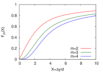
Figure 2: Function $F_{m}(X)$ in Eq. (118). Dependences of all factorial cumulants on $\Delta y$ are proportional to $F_{m}(X)$. The horizontal axis corresponds to the ratio between the rapidity window $\Delta y$ and the diffusion length $d$.

Substituting Eq. (114) into Eq. (107), one obtains

$$\langle n_{\Delta y}^{m}\bar{n}_{\Delta y}^{\bar{m}}\rangle_{\rm fc}=\kappa_{m\bar{m}}\int dy[p_{\Delta y}(y)]^{m+\bar{m}}.$$ (116)

Using Eq. (100), Eq. (116) is calculated to be

$$\frac{\langle n_{\Delta y}^{m}\bar{n}_{\Delta y}^{\bar{m}}\rangle_{\rm fc}}{\Delta y}=\kappa_{m\bar{m}}F_{m+\bar{m}}\Big{(}\frac{\Delta y}{d}\Big{)}$$ (117)

with

$$F_{m}(X)=\frac{1}{\Delta y}\int dz\Big{(}\int_{-1/2}^{1/2}dz^{\prime}\frac{X}{\sqrt{2\pi}}e^{-\frac{(z-z^{\prime})^{2}}{2}X^{2}}\Big{)}^{m}.$$ (118)

In the left panel of Fig. 2, we show $F_{m}(X)$ as functions of $X$ for $m=2,3,4$.

Using the relations in Sec. II.2, the above results for factorial cumulants can be converted into cumulants. These results agree with those in Refs. Kitazawa:2013bta ; Kitazawa:2015ira obtained from the diffusion master equation. The same result for second order is obtained in Ref. Shuryak:2000pd .

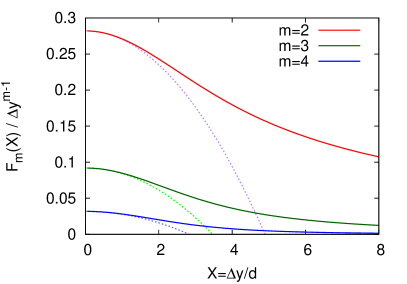
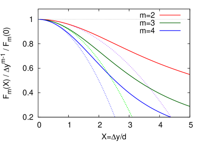
Figure 3: Upper panel shows $F_{m}(X)$ divided by $\Delta y^{m-1}$. In the lower panel the same function is shown in the normalization $(F_{m}(X)/\Delta y^{m-1})/F_{m}(0)$. Dependences of all factorial cumulants on $\Delta y$ are proportional to $F_{m}(X)$. The expansion of $F_{m}(X)$ up to $X^{2}$, Eq. (119), are also shown by dashed lines.

It is instructive to see the behavior of Eq. (117) in the small $\Delta y$ limit. In this limit corresponding to $X\to 0$, $F_{m}(X)$ is expanded as

$$F_{m}(X)=\frac{X^{m-1}}{\sqrt{m(2\pi)^{m-1}}}\Big{(}1-\frac{m-1}{24}X^{2}+{\cal O}(X^{4})\Big{)}.$$ (119)

This result shows that the factorial cumulants have power law behaviors $\langle n_{\Delta y}^{m}\bar{n}_{\Delta y}^{\bar{m}}\rangle_{\rm fc}\sim\Delta y^{m+\bar{m}}$, as pointed out in Ref. Ling:2015yau for the single variable case. Equation (119) also shows that the deviation from the power law behavior is more prominent for higher orders. In Fig. 3, we show $F_{m}(X)$ in the normalizations $F_{m}(X)/\Delta y^{m-1}$ and $(F_{m}(X)/\Delta y^{m-1})/F_{m}(0)$.

VII.4 Implications to experiments

Let us inspect phenomenological implications of the above result.

First, Eq. (117) tells us that the factorial cumulants $\langle n_{\Delta y}^{m}\bar{n}_{\Delta y}^{\bar{m}}\rangle_{\rm fc}$ have a common $\Delta y$ dependence for the same $m+\bar{m}$ with different proportionality coefficients. For example, all the factorial cumulants of proton and anti-proton at fourth order,

$$\langle n_{p}^{4}\rangle_{\rm fc},\ \langle n_{p}^{3}n_{\bar{p}}\rangle_{\rm fc},\ \langle n_{p}^{2}n_{\bar{p}}^{2}\rangle_{\rm fc},\ \langle n_{p}n_{\bar{p}}^{3}\rangle_{\rm fc},\ \langle n_{\bar{p}}^{4}\rangle_{\rm fc},$$ (120)

defined in a rapidity window $\Delta y$ are proportional to $F_{4}(\Delta y/d)$ with the proportionality coefficients $\kappa_{m\bar{m}}$. This behavior can be checked explicitly in experiments. Because Eq. (117) is obtained from the non-interacting Brownian particle model, this experimental analysis serves as a check of the validity of this picture. In Refs. Kitazawa:2013bta ; Kitazawa:2015ira , similar argument has been made only on the basis of the cumulants. The discussion with factorial cumulants enables more quantitative analysis of the $\Delta y$ dependence.

Second, the $\Delta y$ dependences of the factorial cumulants $\langle n_{\Delta y}^{m}\bar{n}_{\Delta y}^{\bar{m}}\rangle_{\rm fc}$ can be used to study the diffusion length $d$ experimentally, by comparing the $\Delta y$ dependences of various factorial cumulants with the form of $F_{m}(X)$ in Fig. 2. The diffusion length is directly connected to the diffusion coefficient, and an important experimental observable to study transport property of the medium. We emphasize that the use of the factorial cumulants with various orders would be helpful in this analysis, because the $\Delta y$ dependence is different for different orders as in Fig. 2.

Third, if the non-interacting Brownian particle model is justified experimentally, one can use the above results to estimate of the susceptibilities in the initial condition, $\chi_{m\bar{m}}$. In this analysis, one first determines $\kappa_{m\bar{m}}$ from the magnitude of $\langle n_{\Delta y}^{m}\bar{n}_{\Delta y}^{\bar{m}}\rangle_{\rm fc}$. The susceptibilities $\chi_{m\bar{m}}$ can then be constructed from $\kappa_{m\bar{m}}$ with Eq. (115). By combining the values of $\chi_{m\bar{m}}$, it is possible to obtain the susceptibility of the conserved charges, such as the one of the net-baryon number. The susceptibility obtained in this way is the quantity which is the most suitable for the comparison with theoretical analyses and lattice QCD simulations.

Finally, we note that the above results are obtained within an idealized setting which would not be justified in real heavy-ion collisions Asakawa:2015ybt . First, although we assumed Bjorken expansion this picture would be violated for lower energy collisions. For lower energy collisions, the effects of global charge conservation Sakaida:2014pya have to be considered seriously, too. Second, our results are obtained with the assumption of locality Eq. (111). When the correlation length is not sufficiently small, this assumption has to be relaxed. As discussed in Ref. Sakaida:2017rtj for second order cumulant, non-equilibrium effects near the critical point also lead to the violation of the locality assumption. Third, other various effects in real heavy-ion collisions Asakawa:2015ybt ; Alba:2015iva ; Feckova:2015qza ; Hippert:2017xoj ; Braun-Munzinger:2016yjz have also be taken into account. We left the inclusion of these effects for future study.

VIII Summary

In the present study, we studied the properties and applications of factorial cumulants in relativistic heavy-ion collisions. The properties of factorial cumulants including those of mixed channels and particles having non-unit charges have been discussed. We showed that these factorial cumulants can be interpreted as the cumulants after removing the effect of self correlation in classical particle systems. Nevertheless, it is also discussed that these properties of factorial cumulants are not so useful in heavy-ion collisions.

We discussed new usages of factorial cumulants for three practical problems in Secs. V, VI, and VII. These arguments are related to the binomial model, which is justified when the underlying probabilistic processes are independent. In the binomial model, factorial cumulants in this model are connected by a simple relation Eq. (90). We showed that this relation plays quite useful roles in the reconstruction of the original cumulants from the incomplete information obtained experimentally. As such examples, we discussed the uses of factorial cumulants in efficiency correction and the studies of $p_{T}$ range and rapidity window dependences of fluctuation observables.

We finally note that the discussions in Secs. V, VI, and VII can be combined, although in this paper we discussed them separately for simplicity. For example, it is possible to deal with the effects of the efficiency of detectors and $p_{T}$ cut simultaneously.

References

- (1) M. Asakawa and M. Kitazawa, Prog. Part. Nucl. Phys. 90, 299 (2016) [arXiv:1512.05038 [nucl-th]].
- (2) M. A. Stephanov, K. Rajagopal and E. V. Shuryak, Phys. Rev. D 60, 114028 (1999) [hep-ph/9903292].
- (3) M. Asakawa, U. W. Heinz, and B. Müller, Phys. Rev. Lett. 85, 2072 (2000) [arXiv:hep-ph/0003169].
- (4) S. Jeon and V. Koch, Phys. Rev. Lett. 85, 2076 (2000) [arXiv:hep-ph/0003168].
- (5) V. Koch, arXiv:0810.2520 [nucl-th].
- (6) X. Luo and N. Xu, arXiv:1701.02105 [nucl-ex].
- (7) S. Ejiri, F. Karsch, and K. Redlich, Phys. Lett. B633 (2006) 275.
- (8) M. A. Stephanov, Phys. Rev. Lett. 102, 032301 (2009) [arXiv:0809.3450 [hep-ph]].
- (9) M. Asakawa, S. Ejiri and M. Kitazawa, Phys. Rev. Lett. 103, 262301 (2009) [arXiv:0904.2089 [nucl-th]].
- (10) B. Friman, F. Karsch, K. Redlich, and V. Skokov, Eur. Phys. J. C 71, 1694 (2011) [arXiv:1103.3511 [hep-ph]].
- (11) M. A. Stephanov, Phys. Rev. Lett. 107 (2011) 052301 [arXiv:1104.1627 [hep-ph]].
- (12) M. Sakaida, M. Asakawa and M. Kitazawa, Phys. Rev. C 90, no. 6, 064911 (2014) [arXiv:1409.6866 [nucl-th]].
- (13) P. Alba, R. Bellwied, M. Bluhm, V. Mantovani Sarti, M. Nahrgang and C. Ratti, Phys. Rev. C 92, no. 6, 064910 (2015) [arXiv:1504.03262 [hep-ph]].
- (14) S. Mukherjee, R. Venugopalan and Y. Yin, Phys. Rev. C 92, no. 3, 034912 (2015) [arXiv:1506.00645 [hep-ph]].
- (15) M. Hippert, E. S. Fraga and E. M. Santos, Phys. Rev. D 93, no. 1, 014029 (2016) [Phys. Rev. D 93, 014029 (2016)] [arXiv:1507.04764 [hep-ph]].
- (16) Z. Fecková, J. Steinheimer, B. Tomášik and M. Bleicher, Phys. Rev. C 92, no. 6, 064908 (2015) [arXiv:1510.05519 [nucl-th]].
- (17) C. Herold, M. Nahrgang, Y. Yan and C. Kobdaj, Phys. Rev. C 93, no. 2, 021902 (2016) [arXiv:1601.04839 [hep-ph]].
- (18) P. Braun-Munzinger, A. Rustamov and J. Stachel, Nucl. Phys. A 960, 114 (2017) [arXiv:1612.00702 [nucl-th]].
- (19) M. Hippert and E. S. Fraga, arXiv:1702.02028 [hep-ph].
- (20) W. Fan, X. Luo and H. Zong, arXiv:1702.08674 [hep-ph].
- (21) G. Almasi, B. Friman and K. Redlich, arXiv:1703.05947 [hep-ph].
- (22) M. Sakaida, M. Asakawa, H. Fujii and M. Kitazawa, arXiv:1703.08008 [nucl-th].
- (23) S. He and X. Luo, arXiv:1704.00423 [nucl-ex].
- (24) B. Abelev et al. [ALICE Collaboration], Phys. Rev. Lett. 110, 152301 (2013). [arXiv:1207.6068 [nucl-ex]].
- (25) L. Adamczyk et al. [STAR Collaboration], Phys. Rev. Lett. 112, 032302 (2014) [arXiv:1309.5681 [nucl-ex]].
- (26) L. Adamczyk et al. [STAR Collaboration], Phys. Rev. Lett. 113, 092301 (2014) [arXiv:1402.1558 [nucl-ex]].
- (27) J. Thäder [STAR Collaboration], Nucl. Phys. A 956, 320 (2016) [arXiv:1601.00951 [nucl-ex]].
- (28) R. Esha [STAR Collaboration], “Measurement of the cumulant of net-proton multiplicity distribution in Au+Au collisions at GeV from the STAR experiment”, talk given at “Quark Matter 2017”, 5-11 February 2017, Chicago, USA.
- (29) A. Rustamov [ALICE Collaboration], “Net baryon fluctuations from ALICE at the LHC”, talk given at “Quark Matter 2017”, 5-11 February 2017, Chicago, USA.
- (30) H. T. Ding, F. Karsch and S. Mukherjee, Int. J. Mod. Phys. E 24, no. 10, 1530007 (2015) [arXiv:1504.05274 [hep-lat]].
- (31) “White Paper” http://asrc.jaea.go.jp/soshiki/gr/hadron/jparc-hi/
- (32) R. Rapp et al., Lect. Notes Phys. 814, 335 (2011). doi:10.1007/978-3-642-13293-3_4
- (33) D. Blaschke, et al., Eur. Phys. J. A 52, 267 (2016).
- (34) M. Kitazawa, M. Asakawa, and H. Ono, Phys. Lett. B 728, 386 (2014).
- (35) M. Kitazawa, Nucl. Phys. A 942, 65 (2015) [arXiv:1505.04349 [nucl-th]].
- (36) B. Ling and M. A. Stephanov, Phys. Rev. C 93, no. 3, 034915 (2016) [arXiv:1512.09125 [nucl-th]].
- (37) A. Bzdak, V. Koch and N. Strodthoff, arXiv:1607.07375 [nucl-th].
- (38) T. Nonaka, M. Kitazawa and S. Esumi, arXiv:1702.07106 [physics.data-an].
- (39) C. Gardiner, Stochastic Methods, Springer, 2009.
- (40) M. Kitazawa and M. Asakawa, Phys. Rev. C 85, 021901 (2012); [arXiv:1107.2755 [nucl-th]];
- (41) M. Kitazawa and M. Asakawa, Phys. Rev. C 86, 024904 (2012) [Erratum-ibid. C 86, 069902 (2012)]. [arXiv:1205.3292 [nucl-th]].
- (42) Y. Ohnishi, M. Kitazawa and M. Asakawa, Phys. Rev. C 94, 044905 (2016) [arXiv:1606.03827 [nucl-th]].
- (43) E. V. Shuryak and M. A. Stephanov, Phys. Rev. C 63, 064903 (2001) [hep-ph/0010100].
- (44) A. Bzdak and V. Koch, Phys. Rev. C 86 (2012) 044904.
- (45) A. Bzdak and V. Koch, Phys. Rev. C 91, no. 2, 027901 (2015) [arXiv:1312.4574 [nucl-th]].
- (46) X. Luo, Phys. Rev. C 91, no. 3, 034907 (2015) Erratum: [Phys. Rev. C 94, no. 5, 059901 (2016)] [arXiv:1410.3914 [physics.data-an]].
- (47) M. Kitazawa, Phys. Rev. C 93, no. 4, 044911 (2016) [arXiv:1602.01234 [nucl-th]].
- (48) F. Karsch, K. Morita and K. Redlich, Phys. Rev. C 93, no. 3, 034907 (2016) [arXiv:1508.02614 [hep-ph]].
- (49) K. Morita and K. Redlich, PTEP 2015, no. 4, 043D03 (2015) [arXiv:1409.8001 [hep-ph]].